IOWA STATE UNIVERSITY Department of Economics Ames, Iowa, 50011-1070

Iowa State University does not discriminate on the basis of race, color, age, religion, national origin, sexual orientation, gender identity, sex, marital status, disability, or status as a U.S. veteran. Inquiries can be directed to the Director of Equal Opportunity and Diversity, 3680 Beardshear Hall, (515) 294-7612.

Student and Teacher Attendance: The Role of SharedGoods in Reducing Absenteeism

Ritwik Banerjee, Elizabeth M. King, Peter Orazem, Elizabeth M.Paterno

Working Paper No. 10038December 2010

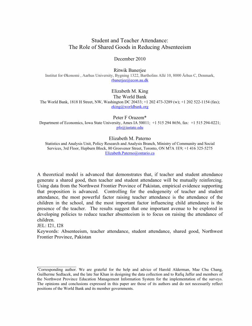
Student and Teacher Attendance: The Role of Shared Goods in Reducing Absenteeism

December 2010

Ritwik Banerjee

Institut for Økonomi , Aarhus University, Bygning 1322, Bartholins Allé 10, 8000 Århus C, Denmark, rbanerjee@econ.au.dk

Elizabeth M. King The World Bank

The World Bank, 1818 H Street, NW, Washington DC 20433; +1 202 473-3289 (w); +1 202 522-1154 (fax); eking@worldbank.org

Peter F Orazem*

Department of Economics, Iowa State University, Ames IA 50011; +1 515 294 8656, fax: +1 515 294-0221; pfo@iastate.edu

Elizabeth M. Paterno

Statistics and Analysis Unit, Policy Research and Analysis Branch, Ministry of Community and Social Services, 3rd Floor, Hepburn Block, 80 Grosvenor Street, Toronto, ON M7A 1E9; +1 416 325-5275

Elizabeth.Paterno@ontario.ca

A theoretical model is advanced that demonstrates that, if teacher and student attendance generate a shared good, then teacher and student attendance will be mutually reinforcing. Using data from the Northwest Frontier Province of Pakistan, empirical evidence supporting that proposition is advanced. Controlling for the endogeneity of teacher and student attendance, the most powerful factor raising teacher attendance is the attendance of the children in the school, and the most important factor influencing child attendance is the presence of the teacher. The results suggest that one important avenue to be explored in developing policies to reduce teacher absenteeism is to focus on raising the attendance of children. JEL: I21, I28 Keywords: Absenteeism, teacher attendance, student attendance, shared good, Northwest Frontier Province, Pakistan ___________________ *Corresponding author. We are grateful for the help and advice of Harold Alderman, Mae Chu Chang, Guilherme Sedlacek, and the late Sar Khan in designing the data collection and to Rafiq Jaffer and members of the Northwest Province Education Management Information System for the implementation of the surveys. The opinions and conclusions expressed in this paper are those of its authors and do not necessarily reflect positions of the World Bank and its member governments.

1

Introduction One of the most vexing obstacles on the path to universal literacy is teacher

absenteeism in developing countries. Poor countries struggle to pay for enough teachers for

their schools, but resources are wasted when teachers shirk their responsibilities. Teacher

absenteeism rates have been found to be quite high in developed countries averaging 19% for

primary school teachers (Chaudhury et al. 2006; Das et al. 2007). The 11% absenteeism rate

in Peru is the lowest of the rates reported, but is still more than double the rates in developed

countries. Furthermore, the national averages mask large variations within countries. In

India where teachers are absent 25% of the time, rates are as high as 42% in the state of

Jharkhand ( Kremer, et al., 2005).

One factor that seems to explain high teacher absenteeism is the lack of adequate

supervision which makes it possible for teachers to shirk without penalty. This problem is

particularly acute in rural areas where supervision might require significant travel, but even

in cities teacher absenteeism can be a serious problem. Contributing to the problem are

generous leave policies that allow teachers to miss 10% or more of the class days. Myriad

other duties take teachers away from the classroom, including training, meetings with

superiors, and administrative responsibilities. In the countries surveyed by Chaudhury et al.

(2004), official leaves and work obligations accounted for between 25% and 86% of the

teacher absences.

However, even in countries with generous leave policies, there is tremendous

variation in attendance rates among teachers. Some will use all their allotment while others

do not use the leaves they are allowed. A number of hypotheses have been advanced to

explain this variation in teacher attendance, including pay, working conditions, opportunities

2

for alternative employment outside teaching, and traveling distance to school. Especially

among female teachers, family responsibilities can also lead to absences. In addition,

inadequate supervision and monitoring insulate teachers from accountability for their

performance (Majumdar, 2001). Studies show that while 35 out of 600 rural private schools

in India reported incidence of teacher suspension due to absence or negligence, only 1 out of

3,000 teachers in rural public schools is suspended for the same reason (Kremer et al. 2005).

Econometric evidence of the determinants of teacher absenteeism in developing

countries is limited, and research has failed to generate consistent results. Chaudhury et al.

(2004, 2006) estimated teacher absenteeism regressions for six countries and found no

variable to be consistently significant across the six regressions. Of the 22 variables

(excluding the constant term and survey wave dummies) used in their multi-country

regressions (Chaudhury et al., 2006), only six were statistically significant despite nearly

35,000 observations. Barely half of those variables had coefficients of the same sign in more

than one-half of the countries. Even teacher salaries do not have consistent effects on teacher

attendance, no doubt because salaries are set by civil service rules and not performance.

Nevertheless, two results emerge consistently in the estimates. Monitoring, as measured by

the school’s proximity to the Ministry of Education and the frequency of recent school

inspections, appears to raise attendance, as does having students with more educated parents.

Several countries have experimented with programs that improve school and teacher

monitoring. In rural EDUCO schools in El Salvador, a community organization was

contracted by the central education agency to be responsible for hiring and firing teachers

and for closely monitoring their performance. Jimenez and Sawada (1999) found that,

compared with non-EDUCO schools, teacher absences and student absences in EDUCO

3

schools were lower. In the state of Rajasthan in India, schools that were required to provide a

photograph of the teacher and students using a digital camera with a time /date feature

improved attendance (Duflo and Hanna 2005). The program resulted in an immediate

improvement in teacher attendance. Teacher absenteeism was halved in the treatment

schools, dropping from an average of 36 percent in the comparison schools to 18 percent in

the treatment schools. In contrast, Kremer and Chen (2001) reported that when school

headmasters in Kenya were given monitoring responsibility, there was no change in teacher

absence.1 The policy implication being drawn from these studies is that strong or high-stakes

incentives such as pay-for-performance may be needed to discourage shirking.

Our study examines another avenue for improving teacher attendance—that teacher

attendance depends on the attitudes and behaviors of students themselves, as reflected by

student attendance. The intriguing possibility we pursue in this paper is that, even in the

absence of close monitoring and extrinsic incentives, teachers attend because their students

show up and students attend because their teachers show up. We couch this possibility in the

context of a matching process between teachers and students in which both parties gain

utility when both show up, but where both have outside options that also provide utility. In

that context, teachers who believe their students are only weakly committed to attend will

have more absences, and children who believe their teacher is prone to shirking will also

shirk. In the Chaudhury et al. (2004) analysis, for example, the attributes of the children and

their parents were at least as important as the attributes of the teachers or the school. That

result should not be surprising in that teacher attendance rates can vary dramatically within a

1 Study by Michael Kremer and David Chen cited in Banerjee and Duflo (2006)

4

country among teachers with standardized contracts, qualifications, curricula, and working

conditions.

We illustrate the performance of this matching process using a unique data set

composed of a representative sample of primary teachers and a random sample of their

students collected in the North West Frontier Province of Pakistan in 1994-95. We find that

by far the most important factor for teacher attendance is a higher probability that their

students attend, and that the most important factor for child attendance is also a higher

likelihood that the teacher will appear. The implication is that policies crafted to increase

child attendance, such as conditional transfer programs that require a specified level of child

attendance, will have the collateral benefit of raising the attendance of the teachers in local

schools. Likewise, policies such as those that give the community some power to monitor

teacher behavior in local schools will have the associated benefit of better student attendance.

The next section lays out a simple model that demonstrates the nature of the match

between the teacher and the child and/or his parents. The theory motivates an empirical

strategy that is outlined in Section III. Section IV gives a detail description of the data while

Section V lays out the results.

5

II. Model

The economic models that have been applied to frame issues regarding teachers

include those that treat teachers’ educational background and years of experience as inputs

into a production function for student achievement;2 those that describe the accountability

relationship between the teacher and the community (made up of local parents and their

children and/or their representatives in school administration);3 and those that focus on the

labor supply behavior of teachers as being one of income optimization constrained by the

disutility from effort exerted.4 While the last model is frequently used to examine why

individuals enter or remain in the teaching profession, the model applies more generally to

teacher choices regarding how much effort to expend.

One aspect of being a teacher that none of these models emphasizes is that teachers

may derive utility from their professional practice beyond the salary they receive. Certainly

many professions may offer hedonic returns in the form of pride of accomplishment or

prestige among ones peers, but a unique aspect of being a teacher is that the process of

instruction and its ultimate output are intrinsically a product of the joint efforts by the teacher

and by the student. We stress this feature of the production process because the concerns

about frequent teacher absences and about irregular attendance by students, as demonstrated

in our literature review, is underpinned by the belief that the teaching-learning process

requires the direct interaction between teacher and student. Thus, when either teacher or

student is absent, the learning process is incomplete. Furthermore, the frequency and duration

2 Glewwe (2002) reviews the educational production literature. 3 Podgursky and Springer (2007) present a review of compensation options to resolve the principal agent problem in education 4 Two early examples of empirical models of teacher labor supply include Theobald (1990) and Stinebrickner (1998).

6

of this interaction contributes to learning because it allows the two parties to know each

other. A teacher doesn’t start off knowing a student’s endowments (e.g., ability to learn,

ability to focus, persistence), and so it may take a few meetings to understand how best to

teach a class. Similarly, a student may need a few classes to get to know and adapt to a

teacher’s style of teaching. This way of framing the teacher-student relationship recognizes

that interaction, cooperation and mutual adjustment are all aspects of the teaching-learning

process.

To capture this joint and cooperative production of learning, we note that teachers and

students are two parties in a mutually beneficial contractual relationship. To model the

teacher-student relationship, we draw on the framework Becker(1974) advanced to model

marriage as well as the extensions by Manser and Brown (1980) and McElroy and Horney

(1981). As with a marriage, teachers and students cooperate to produce a “shared good”

which raises utility for both parties.5 The key feature of a shared good is that it cannot be

produced without the participation of both teachers and students. In the classroom context,

examples of a shared good are the satisfaction from the learning that takes place, a productive

mentor-mentee relationship, and the status conferred by the community to teachers and

students of a well-run school.6 In the model below, we treat attendance (or absences) as a

simple (minimalist) measure of the frequency and quality of the interaction between the

parties.

Let and be the hours the teacher (T) and the child (C) attend such that ,

0,1 . The teacher or student shirk by their absence, setting 1, or 1. We assume 5 The concept of a “shared good” is different from that of a “public good” in the sense when a number of households are created through corresponding matches in the marriage market, a “public good” may be enjoyed by multiple households whereas a “shared good” is enjoyed only within a household. 6 See Coleman (1988), Becker (1974) and Putnam (2000) for classic developments of the social capital concept.

7

that the shared good is produced using a constant elasticity of substitution production process

using student and teacher time. The amount of the shared good, G, produced is

Teacher’s attendance decision

The teacher’s total utility is additive in utility from the shared good, U(G), and goods

purchased with income derived from teaching and other activities. The teacher earns a unit

wage of . Total wages paid to a nonshirking teacher will be . An observed

absence results in forfeiture of income for the period the teacher is absent. On the other

hand, time away from school has value of to the teacher, either because the teacher has

an alternative job or because the teacher values time in home production. We assume that for

the (1 share of time the teacher is absent, s/he earns 1 working away from

school. Consequently, if the teacher shirks and is caught, wage income is

1 .

As is often the case in developing countries, teachers’ attendance is monitored with

error7. If the teacher shirks and is not caught his income is 1 .

More generally, let the teachers’ absence be observed by a supervisor with probability .

Then the teacher’s expected income from shirking will be 1 1

1 . The nonshirking wage is a special case of this formulation, as setting 1

implies that the expected income is .

7 In a study on students dropout at Northwest Frontier Province in Pakistan King, Orazem and Paterno found in a spotcheck that 20% of the teachers were absent, the official attendance however showed only 5% were absent. (King, et al., 1999)

8

Assuming the child’s time in school is given, the teacher’s decision is to select so

as to maximize expected utility,

max 1 1 1 / .

The teacher’s first-order condition is

1

where the left-hand-side of the inequality is the marginal utility the teacher derives from

devoting time to school, equal to the gain from the generated shared good plus the expected

teacher income from reduced chance of being caught shirking; and the right-hand-side is the

value of time from shirking full time. The teacher would set 0 and never attend if the

inequality is violated so that the benefit of any time spent in school is never greater than that

spent outside school. At the other extreme, the teacher sets 1 and always attends if the

marginal utility of shared good plus expected income from attendance is greater than the

value of time away from school. More generally, condition (1) holds with equality and so the

teacher will spend at least some time shirking. Shirking increases as the probability of being

caught decreases, as the value of time out of school increases, and as teacher salary and the

marginal utility of the shared good decreases. Assuming an interior solution, the teacher’s

equation governing time allocated to school will be of the form:

, , , 2

Child’s attendance decision

The child’s attendance choice, or that of the parent acting on behalf of the child,

involves selecting so as to maximize expected utility. The child has an opportunity cost of

time spent in school, , that represents the larger of either the value of time spent in home

9

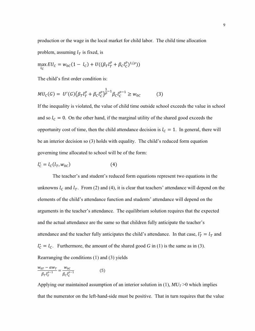
production or the wage in the local market for child labor. The child time allocation

problem, assuming is fixed, is

max 1 /

The child’s first order condition is:

3

If the inequality is violated, the value of child time outside school exceeds the value in school

and so 0. On the other hand, if the marginal utility of the shared good exceeds the

opportunity cost of time, then the child attendance decision is 1. In general, there will

be an interior decision so (3) holds with equality. The child’s reduced form equation

governing time allocated to school will be of the form:

, 4

The teacher’s and student’s reduced form equations represent two equations in the

unknowns and . From (2) and (4), it is clear that teachers’ attendance will depend on the

elements of the child’s attendance function and students’ attendance will depend on the

arguments in the teacher’s attendance. The equilibrium solution requires that the expected

and the actual attendance are the same so that children fully anticipate the teacher’s

attendance and the teacher fully anticipates the child’s attendance. In that case, and

. Furthermore, the amount of the shared good G in (1) is the same as in (3).

Rearranging the conditions (1) and (3) yields

5

Applying our maintained assumption of an interior solution in (1), MUT >0 which implies

that the numerator on the left-hand-side must be positive. That in turn requires that the value

10

of a teacher’s time away from school must exceed the expected lost wage from being caught

shirking. Because both sides of equation (5) are positive, we know that any factor that raises

teachers’ attendance will also increase students’ attendance, and so there will be a positive

correlation between their attendance decisions. We will test these predictions in the empirical

work below.

III. Empirical Strategy

We are interested in estimating equations (2) and (4) from our theory. The linear

approximation to the functional form in (2) is

6

The specification shows that teacher attendance will depend on student attendance and

measures of the teacher’s expected return from spending time inside and outside of class. The

teacher’s compensation includes the teacher’s salary and also working conditions such as

the availability of furniture in the school, commuting distance from home to school, and

whether the teacher has head teacher or other supervisory responsibilities besides teaching.

The teacher’s incentive to attend school will also reflect the likelihood of being caught

shirking, . The chance of being caught increases with the degree of supervision which will

be stricter in private schools and would also likely vary with the number of other teachers in

the school.8 Attendance will also vary negatively with factors that raise the value of teacher

time outside school, holding constant the salary paid in the school. These include the

teacher’s human capital (age and education) and the factors that alter the value of time in

household production (gender, marital status, and number of young children). 8 Fewer teachers can make collusive arrangements to share attendance, and more teachers would mean more chances of being observed absent. Nevertheless, one of the authors recalls a series of school visits in which the one teacher schools had one teacher present; the two teacher school had one teacher present and the three teacher school had one teacher present.

11

The linear approximation to (4) provides an equation explaining child attendance

7

The child’s attendance will depend on the teacher’s attendance and on the value of the child’s

time outside, relative to the value inside, school. The relative value of time inside versus

outside class depends on school amenities such as furniture, class size, and teacher attributes

and on child age, gender, health and home attributes (parent and sibling demographics,

wealth, and distance from school).

We could estimate (6) and (7) directly if we assume that child attendance is

exogenous to the teacher and teacher attendance is exogenous to the child. The theory

suggests, however, that this exogeneity assumption is not credible. The existence of a shared

good between teachers and students is consistent with positive estimates of the coefficients

and . Therefore, we propose two alternative strategies to test for evidence of a positive

correlation between teacher and student attendance consistent with a shared good.

First, consider the projection of the teacher’s and child’s attendance on their own

exogenous variables

(8A)       (8B) 

 The error term is orthogonal to all teacher household and school attributes, and the error

term is be orthogonal to child household and school attributes. We can then examine

whether COV( , > 0 to establish whether the unobservable factors raising teacher and

student attendance are positively correlated as suggested by the theory.

The other strategy is to use (8A) and (8B) to suggest instruments for and

in (6) and (7), yielding the structural equations

12

| (9A)

| , , (9B)

Estimating (8A,B) and (9A,B) simultaneously provides unbiased estimates of the coefficients

and which must be positive to be consistent with the prediction from the theory.

IV. Data

Survey Characteristics

A sample of 257 primary schools was selected from a population of over 20,000 schools in

NWFP, Pakistan. Sixty-eight percent of the selected schools were situated in rural areas,

with school management divided between government schools (76%), mosque schools (7%),

and private schools (17%), in proportion to their presence among the universe of schools.

The data collection occurred during the spring of 1994.

At each school, a teacher from each of the first three grades was selected at random.

In schools with fewer than four teachers in the first three grades, all teachers were sampled.

A total of 650 teachers were interviewed from 257 schools to obtain information on teacher

household and school attributes. Information on teachers’ absence was obtained from two

sources- the official attendance register kept at the school and a spot check of teacher

attendance conducted during unannounced visits to the school.

In each of the teachers’ classes, two children were selected at random for the child

attendance sample. For each child, daily attendance from the attendance register was

obtained as well as a spot check on the same day as the teacher. For each child, an

interviewer was dispatched to the household to administer a detailed survey of household

demographics and socioeconomic status.

13

Dependent Variables

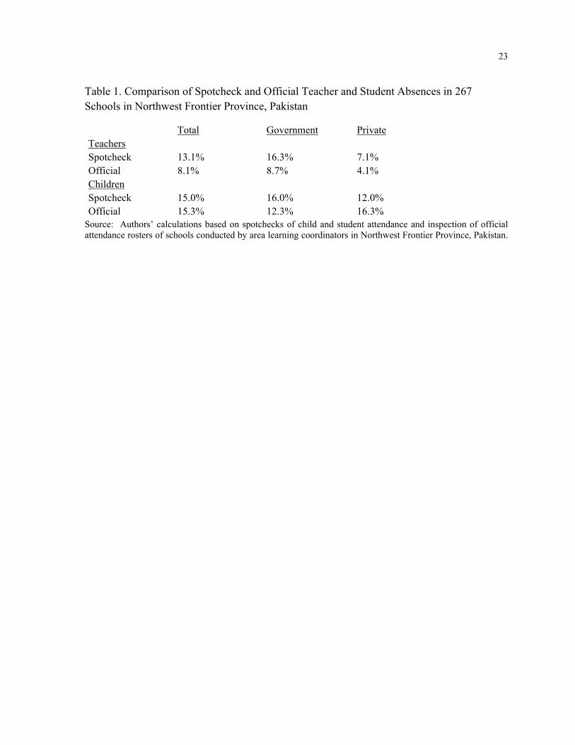
Because of the possibility that official attendance was inconsistent with actual

attendance, we conducted spot checks of teacher and student attendance and compared them

with the attendance records kept at the school. The comparison is reported in Table 1.

Because the register contains attendance over several months and the spot check data were

collected on only two days, the two series may not coincide exactly, but there are some clear

discrepancies in the teachers’ official attendance records. For both private and government

schools, official absences greatly understate the true absences of teachers, especially in

government schools. However, the official attendance information for students coincides

reasonably well overall. In addition, surveyors checked if the students listed as present were

indeed in school that day, and they reported reasonable accuracy of student presence or

absence. The same could not be said for teachers, numerous discrepancies were found

between reported attendance and the spot check. We use the teachers’ spot check attendance

as our dependent variable for the teachers’ equation and the official attendance register data

for the students.9

Independent Variable Selection

The theory suggested three factors that influence whether a teacher shows up in school on a

given day. We assign variables from the surveys that reflect these variables. Note that some

may fit in more than one category.

9 There is a danger in using the spot check for both in that absent teachers may cause absent students. Interestingly, the surveyors found that even when teachers were absent, the present teachers were very careful to take accurate attendance data for the students including those students in the classrooms of the absent teachers.

14

• : incentives to atte . The most obvious incentive to attend is the teacher’s

salary. However, the teacher may still be paid, even if the teacher shirks.10 School

furnishings such as desks, chairs, and blackboards affect the quality of the work

environment. Some teachers are given administrative responsibilities beyond their

teaching which can also affect the quality of the job.

• : the opportunity cost of time in school. One likely source of higher

opportunity cost of attendance will be due to household responsibilities. Teachers

who are married and who have children under age five have greater value of time

in the home. Commuting time from the teacher’s home to school raises the cost of

attendance. Finally, noting that the teacher’s salary is also included in the

regressors, teacher’s with greater endowments of skill that are valued outside

school will have alternative earning possibilities outside school. We include the

teacher’s age and education.

• : The probability of being caught shirking. Schools with more teachers have

greater opportunity to pass on responsibilities to another teacher, but there are also

more difficulties in establishing collusive agreements on shirking. Private schools

are reputed to have closer supervision and no constraints on dismissal which

increases the costs of shirking.

For the child’s attendance equation, the key issue is the relative value of child time out of

school versus in school.

10 The Pakistan teacher contract lists many legal reasons to skip that may allow the teacher to be absent 20% of the time or more and still earn full pay. Legal absences include sickness, official business, maternity, earned vacation, training, and up to 25 days of “casual leave” for which no reason is necessary.

15

II. : the opportunity cost of child time. A child’s productivity outside relative to

inside school will reflect the child’s age, health and gender. Having more siblings

in the home can affect both ability to pay for schooling and represent an

additional need for child time. The presence and abilities of parents affect the

ability of the household to produce without using children to produce. Similarly,

household wealth, measured as the first principal component of a vector of

household asset measures, indicates the ability of the household to afford devoting

child time to school.11 Finally, commuting time from home to school increase the

cost of devoting child time to school. School quality is indexed by school

furnishings and whether the school is under private versus government

management.

V. RESULTS

Our model suggests that there will be a strong correlation between teachers’

attendance and that of their students. The simple correlation is 0.47, although ione might

suspect that is due to common school attributes.

To investigate the interrelationship between child and teacher attendance more

carefully, we report results of the teachers’ attendance equations in Table 3 and the students’

equations are given in Table 4. The first column in each table reports the coefficients from

ordinary least squares (OLS) estimation of equations (8A) and (8B). The key take away from

those estimates is how little of the variation in teacher and child attendance can be explained

11 We follow Filmer and Pritchett (2001) in aggregating a large vector of household attributes into a single measure. The thirteen household attributes include measures of the quality of home construction; availability of telephone, water, sewer and electricity; household human capital including measures of occupation and literacy; and possession of various household appliances and electronics.

16

by their own household and school information. The teachers’ demographic household and

school information explains only 8% of the variation in teacher attendance while the

children’s demographics, household attributes and school characteristics only explain 6% of

the children’s attendance variation. The error term from the teachers’ regression will be

orthogonal to teachers’ demographic, household and school attributes while the error terms

from the children’s regression will be orthogonal to the children’s demographic, household

and school attributes. Nevertheless, the teacher and child errors are correlated at 0.41. The

unobserved heterogeneity (to the econometrician) in child and teacher attendance are

significantly positively correlated.

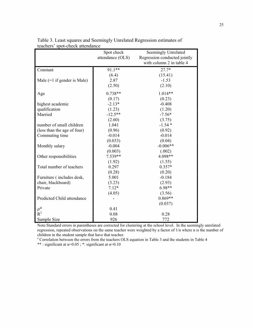
Equations (9A) and (9B) provide a structural model that will allow us to directly

estimate the effect of predictable teacher attendance on child attendance and predictable child

attendance on teacher attendance. We estimate the system jointly using seemingly unrelated

regression. The results are reported in the second columns of Tables 3 and 4, respectively.

However, we first estimated each of the equations independently to derive a measure of the

attendance variation that can be explained when we add the predicted child attendance to the

teachers’ equation and the predicted teachers’ attendance to the children’s equation. The

increase in the R2 is dramatic. Adding predicted child’s attendance to the teachers’ equation

raises the percent of explained variation in teachers’ attendance from 8% to 28%. Adding

predicted teacher attendance in to the model explaining the students’ attendance raises the

percent of explained variation from 6% to 25%. It seems apparent that attendance is a joint

decision between teachers and students, consistent with the prediction suggested by equation

(5).

17

The key parameter in Table 3 is that on children’s attendance that is predicted on

knowledge of the children’s home environments and characteristics of the school. The

coefficient of 0.87 is highly significant and suggests that 100% child attendance will raise the

teachers’ attendance by 87 percentage points. At sample means, the elasticity is 0.83, and so

a 10% increase in child attendance raises teacher attendance by 8.3%. The key parameter in

Table 4 is that on teachers’ attendance that can be predicted from knowledge of the teacher’s

household attributes and characteristics of the school. The coefficient is 0.39 and highly

significant with an implied elasticity of 0.41. A 10% increase in teacher attendance increases

child attendance by 4%. There are no other factors that matter more for teacher attendance

than the attendance of their students, and there is no large influence on child attendance than

the consistent presence of the teacher. Policies that encourage the attendance of one will

increase the attendance of the other.

For example, conditional transfer programs have been shown to increase how

regularly children attend school in Latin America. Our results suggest that conditional cash

transfers aimed at raising children’s attendance will also increase how regularly teachers

attend. Alternatively, the use of date-time digital cameras increases the attendance of

teachers in rural India. Our results suggest that children in those communities will attend

more regularly as well.

For the other variables, there are several avenues where policy could increase teacher

attendance suggested by the results in Table 3. Family responsibilities appear to exacerbate

teacher absenteeism, given the negative effects of teacher marital status and children on

attendance. Attendance is greater in larger schools, presumably because of better monitoring

of teacher attendance. Attendance is significantly higher in private schools where monitoring

18

is greater and punishment for absenteeism more severe. Finally, teachers who have more

administrative responsibilities attend more regularly as well. Our results show that policies

that raise teacher attendance will increase time children spend in school.

The regressions in Table 4 do not provide clear policy avenues to raise children’s

attendance. It is clear that children attend private school more regularly, and other studies

have demonstrated that in Pakistan, even low fee private schools generate better cognitive

outcomes than government schools (Alderman et al., 2001). Experimental work has shown

that a girls school scholarship program that tied a tuition payment to attendance raised girls’

attendance significantly in Balochistan Province of Pakistan (Kim et al., 1999; Alderman et

al., 2003), and perhaps that is an avenue that could be explored in future research.

VI. Conclusion

This paper develops a theoretical model that shows that teacher and student

attendance are intimately entwined and thus they base their own attendance decision on the

predicted attendance of the other. The production function for learning in the classroom does

require inputs of time from both teacher and student, so teacher performance and student

performance are closely associated. Research shows that, especially in the early schooling

years, the quality and frequency of the interaction between teacher and student lead to more

learning (e.g., Martin and Dowson 2009). For this reason, governments and school

administrators use a variety of incentives to elicit better performance from teachers.

We propose that the interaction between teacher and student produces a shared good

which serves as an additional motivation for both the teacher and the student not to be absent.

The existence of this motivation means that a weaker incentive than those being tried by

governments (e.g., performance-linked pay, cash rewards for attendance, contract tenure for

19

teachers)12 may suffice to improve teacher attendance as long as students come to school

regularly. Thus, programs that raise student attendance (especially if those entail lower

additional cost) would have the effect of raising teacher attendance as well. While the shared

good is unobservable, its existence creates a positive correlation in the error terms of

equations explaining student and teacher attendance based solely on their own attributes and

those of the school. We verify that prediction using data on teacher and student attendance

from primary schools in Northwest Frontier Province of Pakistan. We also find evidence

consistent with a second prediction: a dramatic increase in the fit of models of teacher

attendance when we add predicted child attendance, and similarly, a dramatic increase in the

explained variation in child attendance when predicted teacher attendance enters the model.

12 See, for example, Glewwe, Ilias and Kremer (2010), Podgursky and Springer (2007), and Muralidharan and Sundararaman (2010).

20

References Alderman, Harold, Peter Orazem, and Elizabeth Paterno. 2001. “School Quality, School Cost, and the Public/Private School Choices of Low-Income Households in Pakistan.” Journal of Human Resources 36(2):304-326. Alderman, Harold, Jooseop Kim and Peter F. Orazem. 2003. “Design, evaluation, and sustainability of private schools for the poor: the Pakistan urban and rural fellowship school experiments.” Economics of Education Review 22:265-274 Banerjee, Abhijit and Esther Duflo. 2006. “Addressing absence”. Journal of Economic Perspectives 20(1):117-132. Becker, Gary S. 1973. “A Theory of Marriage: Part I.” Journal of Political Economy 81(4):813-846.

Becker, Gary S. 1974a. “A Theory of Marriage: Part II.” Journal of Political Economy 82(2 pt. 2):S11-S26.

Becker, Garry S. 1974b. “A Theory of Social Interactions.” Journal of Political Economy 82(6): 1063-1093. Chaudhury, Nazmul, Jeffrey Hammer, Michael Kremer, Karthik Muralidharan and Halsey F Rogers. 2004. “Provider Absence in Schools and Health Clinics.” World Bank Development Reseach Group Working Paper. Chaudhury, Nazmul, Jeffrey Hammer, Michael Kremer, Karthik Muralidharan and Halsey F Rogers. 2006. “Missing in Action: Teacher and Health Worker Absence in Developing Countries.” Journal of Economic Perspectives 20(1): 91-116.

Chaudhury, Nazmul, Jeffrey Hammer, Michael Kremer, Karthik Muralidharan and Halsey F Rogers. 2004. “Roll Call: Teacher Absence in Bangladesh”. Report: DFID, Government of United Kingdom.

Coleman, James S. 1988. "Social Capital in the Creation of Human Capital." American Journal of Sociology Supplement 94: S95-S120.

Das, Jishnu, Stefan Dercon, James Habyarimana and Pramila Krishnan. 2007. "Teacher Shocks and Student Learning: Evidence from Zambia," Journal of Human Resources 42(4): 820-862. Filmer, D. and H. Pritchett. 2001. “Estimating wealth effects without expenditure data--or tears: an application to educational enrollments in states of India.” Demography 38(1):115-32.

21

Glewwe, P., N. Ilias, and M. Kremer. 2010. “Teacher Incentives,” American Economic Journal: Applied Economics 2 (July): 205–227. http://www.aeaweb.org/articles.php?doi=10.1257/app.2.3.205

Kim, Jooseop., Harold Alderman and Peter F. Orazem. 1999. “Can private school subsidies increase enrollment for the poor? The Quetta Urban Fellowship Program,” World Bank Economic Review 13:443-465.

King, Elizabeth M. and B. Ozler. 2001. “What's Decentralization Got To Do With Learning? Endogenous School Quality and Student Performance in Nicaragua.” Development Research Group Project, World Bank.

Kremer, Michael, Nazmul Chaudhury, Halsey F Rogers, Karthik Muralidharan and Jeffrey Hammer. 2005. “Teacher Absence in India: A Snapshot.” Journal of European Economic Association 3(2-3): 658-67.

Majumdar, Manabi. 2001. “Educational Opportunities in Rajasthan and Tamilnadu: Despair and Hope” in Elementary Education in India: A Grassroots View. eds A. Vaidyanathan and P. R. Gopinathan. SAGE Publications.

Manser, M. and M. Brown. 1980. “Marriage and Household Decision-Making: A Bargaing Analysis” International Economic Review 21(1):31-44.

Martin, A. J. and M. Dowson. 2009. “Interpersonal Relationships, Motivation, Engagement, and Achievement: Yields for Theory, Current Issues, and Educational Practice,” Review of Educational Research 79 (1): 327-365

McElroy, M. B. and M. J. Horney. 1981. “Nash Bargained Household Decisions:Toward a Generalisation of the Theory of Demand.” International Economic Review 22(2):333-49.

Muralidharan, K. and V. Sundararaman. 2010. “The Impact of Diagnostic Feedback to Teachers on Student Learning: Experimental Evidence from India,” The Economic Journal, 120 (August), F187–F203 Podgursky, Michael J. and Matthew G. Springer. 2007. “Credentials versus Performance: Review of the Teacher Performance Pay Research.” Peabody Journal of Education, 82(4), 551–573 Putnam, Robert. 2000. Bowling Alone. The Collapse and Revival of American Community New York: Simon and Schuster.

Stinebrickner, Todd R. 1998. “An empirical investigation of teacher attrition.” Economics of Education Review 17(2): 127-136

22

Theobald, Neil D. 1990. “An examination of the influence of personal, professional, and school district characteristics on public school teacher retention.” Economics of Education Review 9(3): 241-250

23

Table 1. Comparison of Spotcheck and Official Teacher and Student Absences in 267 Schools in Northwest Frontier Province, Pakistan

Total Government Private Teachers Spotcheck 13.1% 16.3% 7.1% Official 8.1% 8.7% 4.1% Children Spotcheck 15.0% 16.0% 12.0% Official 15.3% 12.3% 16.3%

Source: Authors’ calculations based on spotchecks of child and student attendance and inspection of official attendance rosters of schools conducted by area learning coordinators in Northwest Frontier Province, Pakistan.

24

Table 2. Summary Statistics of Variablesa

Variable Mean Std. Dev.

Type Description

Teachers : Explanatory variables and Moments Age 30.6 0.27 Age of the teachers Male 0.66 0.02 D =1 if the teacher is Male Highest academic qualification

3.72 0.03 C Six categories includedb

Married 1.61 0.03 C Two Categoriesc

Number of small children

0.92 0.04 Less than the age of four

Commuting time 30.9 1.02 In minutes Monthly salary 1896 20.5 In Rupees Other responsibilities 0.38 0.01 D Responsibilities other than teaching Schools : Explanatory Variables and Moments Number of Teachers 4.92 3.94 Total teachers in the primary school Furniture 0.50 0.35 Includes toilet, black-board, chairs and

tables Private 0.17 0.38 D =1 if privately owned Children : Explanatory variables and Moments age 7.41 1.38 Age of the student Male 0.67 0.47 D =1 if gender is Male Healthy 0.95 0.22 =1 if student is healthy Distance from school 1.35 3.05 In kilometer Siblings 3.88 1.94 Number of brothers and sisters Dad present 0.91 0.28 D =1 if present Mom present 0.94 0.25 D =1 if present Education of dad 4.62 5.05 Education of mom 0.94 2.46 Wealth 5.44 3.90 Index of wealth created from household

interview Dependent Variable

Teachers’ Attendance 86.9 31.1 D =100 if the Teacher is present on two spotchecks

Children’s Attendance 84.7 18.9 =100 if the child attends full time on the attendance register

aVariable Type:, “D” refers to Dummy and “C” refers to Categorical b1≡6th Grade Pass, 2≡8th Grade Pass, 3≡Matric,4≡FA/FSc,5≡BA/Bsc,6≡MA/Msc c1≡Never married, 2≡Married, Widowed

25

Table 3. Least squares and Seemingly Unrelated Regression estimates of teachers’ spot-check attendance

Spot check attendance (OLS)

Seemingly Unrelated Regression conducted jointly

with column 2 in table 4 Constant 91.1**

(6.4) 27.7*

(15.41) Male (=1 if gender is Male) 2.87

(2.50) -1.53 (2.10)

Age 0.738** (0.17)

1.014** (0.23)

highest academic qualification

-2.13* (1.23)

-0.408 (1.20)

Married -12.5** (2.60)

-7.56* (3.75)

number of small children (less than the age of four)

1.041 (0.96)

-1.54 * (0.92)

Commuting time -0.014 (0.033)

-0.014 (0.04)

Monthly salary -0.004 (0.003)

-0.006** (.002)

Other responsibilities 7.539** (1.92)

4.098** (1.55)

Total number of teachers 0.297 (0.28)

0.357* (0.20)

Furniture ( includes desk, chair, blackboard)

5.001 (3.23)

-0.184 (2.93)

Private 7.12* (4.05)

6.98** (3.56)

Predicted Child attendance - 0.869** (0.037)

0.41 R2 0.08 0.28 Sample Size 926 772 Note:Standard errors in parentheses are corrected for clustering at the school level. In the seemingly unrelated regression, repeated observations on the same teacher were weighted by a factor of 1/n where n is the number of children in the student sample that have that teacher. a Correlation between the errors from the teachers OLS equation in Table 3 and the students in Table 4 ** : significant at α=0.05 ; *: significant at α=0.10

26

Table 4. Least squares and Seemingly Unrelated Regression estimates of Students’ spot-check attendance OLS Seemingly Unrelated

Regression conducted jointly with column 2 in table 4.

Constant 78.2** (6.24)

43.3** (5.68)

Male (=1 if gender is Male) -1.61 (1.42)

1.595 (1.28)

Age -0.66 (0.44)

-0.086 (0.35)

Healthy -0.077 (2.80)

-2.559 (2.47)

Distance from school 0.19 (0.21)

0.053 (0.29)

Siblings -0.46 (0.33)

0.039 (0.29)

Dad present 7.08** (3.06)

1.122 (2.51)

Mom present 7.64* (3.96)

6.266 (4.06)

Education of dad -0.035 (0.14)

0.182 (0.13)

Education of mom 0.056 (0.27)

-0.006 (0.26)

Wealth 0.114 (0.18)

0.011 (0.17)

Furniture ( includes desk, chair, blackboard)

-1.964 (2.01)

-2.21 (1.99)

Private 8.247** (1.96)

4.039** (2.13)

Predicted Teacher Attendance - 0.387** (0.02)

0.41

R² 0.06 0.25 Sample Size 962 772 Note:Standard errors in parentheses are corrected for clustering at the school level. In the seemingly unrelated regression, repeated observations on the same teacher were weighted by a factor of 1/n where n is the number of children in the student sample that have that teacher. a Correlation between the errors from the teachers OLS equation in Table 3 and the students in Table 4 ** : significant at α=0.05 ; *: significant at α=0.10