Government Revenue Stabilization Funds — Do They Make Us Better Off?

Stuart Landon and Constance Smith

Department of Economics University of Alberta Edmonton, Alberta Canada T6G 2H4

.

Author emails: Stuart.Landon@ualberta.ca; Constance.Smith@ualberta.ca.

Keywords: fiscal rules; revenue volatility; resource revenues; stabilization funds; savings funds.

Government Revenue Stabilization Funds — Do They Make Us Better Off?

Abstract

Alberta government resource revenues are highly volatile. Adjustment of government spending to shifts in revenues imposes social and economic costs. To limit the impact of revenue volatility, many jurisdictions have established revenue stabilization funds. There is little empirical evidence on whether these funds improve welfare or whether some fund designs increase welfare by more than others. We provide a quantitative welfare comparison of several different types of rule-based government resource revenue stabilization funds using data for Alberta. Our results show that, relative to the historical path of expenditures, some stabilization funds would have increased welfare. The best performing fund from a welfare perspective requires 50 percent of natural resource revenues to be deposited in the fund each year, and 25 percent of the assets withdrawn. This fund cuts expenditure volatility by almost 30 percent. Stabilization funds that accumulate large asset stocks and, thus, generate low levels of current government services, generally yield low welfare. Funds that depend on an equally-weighted moving average of past revenues have the worst welfare performance of the funds considered. While this study employs data for Alberta, the results are relevant to other resource producing jurisdictions with volatile revenues. .

Keywords: fiscal rules; revenue volatility; resource revenues; stabilization funds; savings funds.

1

1. Introduction

Non-renewable natural resources were the source of almost one-third of Alberta government

revenues over the past 40 years. Resource prices are highly volatile and difficult to predict, so

government non-renewable resource revenues are also volatile and uncertain. Alberta’s non-renewable

resource revenues are twice as variable as corporate income tax revenues and four times more variable

than personal income tax revenues. The large contribution of resource revenues to total Alberta

government revenues, in conjunction with their volatility, causes Government of Alberta revenues to

be twice as variable as the revenues of Ontario, British Columbia and Saskatchewan (Landon and

Smith, 2010). The volatility and uncertainty of government revenues are the focus of considerable

debate in Alberta, and three government studies over the past decade have recommended the

establishment of some type of stabilization or savings fund to address these issues (Tuer, 2002; Mintz,

2007; Emerson, 2011).1 While many countries and US states utilize revenue stabilization funds, there

is surprisingly little empirical research on whether these funds improve welfare or if some types of

funds increase welfare more than others. We fill this gap in the literature by quantifying the impact on

welfare of different types of rule-based commodity revenue stabilization funds using data for Alberta.

While the analysis focuses on Alberta, the results are relevant to resource-based jurisdictions in

Canada and abroad.2

Adjustment to large unpredictable government revenue movements can involve economic,

social and political costs.3 Volatile revenues may induce volatile movements in government

expenditures, leading to stop-go pro-cyclical fiscal policies that accentuate the magnitude of economic

cycles (Boothe, 1995; Sturm et al., 2009; Villafuerte and Lopez-Murphy, 2010; Erbil, 2011).4 The

volatility of economic activity and the volatile provision of government services reduce individual

welfare if consumers prefer less variable income and consumption. If governments increase spending

1 Public debate on the volatility of health and education spending is particularly loud, as indicated by the following comments from rally organizer Vanessa Sauve: “From year to year, things can change depending on what the economy does . . . , but children still need to go to school every year and school boards still have budgets that they need to deal with every year. Unfortunately, it's too tumultuous, and year to year we don't know what's going to happen. . . . Funding needs to be adequate, we want it to be predictable and we want it to be long-term – so not tied in to the oil and gas sector.” (“Rally calls for steady education funding”, CBC News, 29 May 2011.) 2 Natural resource revenues are predicted to account for more than 30 percent of own source government revenues and more than 25 percent of total revenues in both Saskatchewan and Newfoundland during the 2011/12 fiscal year, according to provincial budget documents. Several US states (Alaska, North Dakota, Wyoming, Montana, New Mexico, Oklahoma, Louisiana) are also heavily reliant on non-renewable resource revenues, as are many countries. Non-renewable natural resource revenues comprise more than 25 percent of government revenues in 50 countries, and are an even larger share of revenues in most petroleum producing countries (Venables, 2010). 3 These costs are discussed in more detail in Landon and Smith (2010). Lane (2003) reviews arguments on the optimal cyclicality of government expenditures. 4 Accentuating economic cycles may be costly. Countries with highly variable terms of trade are observed to have slower growth rates, possibly due to the costs of shifting resources between expanding and contracting sectors (Ramey and Ramey, 1995; Blattman, Hwang and Williamson, 2007; van der Ploeg and Poelhekke, 2009).

2

during revenue booms, they compete with the private sector for inputs, which can raise both public and

private sector costs. The volatility of government revenues also creates uncertainty for the private

sector since it is harder to predict future government tax and spending policies. Rapid increases in

government expenditures during booms can stretch the ability of the government to monitor spending,

leading to waste, inefficiency and the unproductive use of government funds (Barnett and Ossowski,

2002). During a revenue collapse, it is often difficult for governments to cut spending efficiently; that

is, to first cut projects and services with the lowest taxpayer benefit. Large expenditure cuts may also

damage the morale and capacity of the public sector, leading to the more inefficient provision of public

services. To the extent that it is easier politically to raise government spending in booms than to

reduce spending in recessions, revenue volatility may lead to the expansion of government and the

implementation of an unsustainable fiscal plan.5

Given the costs associated with volatile expenditures, and the evidence that government

discretionary choices appear to be unable to smooth expenditures when natural resource revenues are

volatile, many commodity-producing jurisdictions have established commodity revenue stabilization

funds as a practical, rule-based method of smoothing expenditures.6 With a stabilization fund, a

portion of commodity revenues are saved in the fund when receipts are strong, and income from the

fund is used to support government spending when resource revenues are low.

As a method of reducing government expenditure volatility, stabilization funds have several

attractive characteristics. Funds are generally easy to implement and explain to the public. Bacon and

Tordo (2006) argue that formal rules for stabilization fund deposits and withdrawals facilitate public

scrutiny and inform the debate on fiscal choices. Wagner and Elder (2005) find US states with rule-

bound budget stabilization funds experience less expenditure volatility, while a recent IMF study notes

that rules that are transparent and backed by appropriate fiscal institutions promote better fiscal

performance (Kumar, Baldacci, Schaechter 2009). An added benefit of a stabilization fund is that,

with clear rules, governments need not identify conditions under which it is appropriate to make

deposits and withdrawals. Further, since commodity price forecasts are highly uncertain, funds can be

designed so that policymakers do not need to forecast future energy prices or determine whether a

5 Frankel (2011) finds that it is common for governments to unrealistically extrapolate booms into the future. Kneebone and McKenzie (2000) report that, over the period 1962-1993, unexpected increases in revenue tended to be treated as permanent by Alberta budget-makers, and led to expenditure increases, while unexpected decreases in revenues tended to be treated as temporary and caused no corresponding spending reduction. The interviews conducted by Boothe (1995) support these conclusions. 6 Descriptions and a discussion of the stabilization funds used in a variety of countries can be found in Davis, Ossowski, Daniel and Barnett (2003) and Ossowski, Villafuerte, Medas and Thomas (2008).

3

change in energy prices is transitory or permanent.7 Stabilization funds can also reduce revenue

uncertainty since revenues, net of fund deposits and withdrawals, depend on past contributions to the

fund and the long-term earnings of the fund. As a result, governments have considerable information

on the future path of transfers from the fund to general revenue and can use this information to plan

expenditures.8 Finally, by providing a smoother revenue stream to government, a stabilization fund

may prevent cyclical tax rate changes. As noted by Barro (1979), this may eliminate the incentive to

concentrate market activity in periods with temporarily low tax rates and, thus, improve economic

efficiency.

While a stabilization fund may be a useful method of addressing volatile and uncertain

revenues, it is not clear that all fund designs, in terms of the rules used to determine deposits and

withdrawals, are equally attractive from a welfare perspective. Many of the stabilization funds used by

resource-producing jurisdictions have been significantly altered or abandoned, which suggests these

funds were not well designed.9 There is very little empirical research on how fund characteristics

affect fund performance. Wagner and Elder (2005) and Sobel and Holcome (1996) find that a fund can

increase fiscal stabilization, but do not address the question of whether alternative fund structures

could yield greater stabilization, nor do they quantify the welfare impact of a fund. Arrau and

Claessens (1992) and Bartsch (2006) employ Monte Carlo simulations to determine optimal

government saving in the presence of commodity price shocks, but also do not make welfare

comparisons across funds. In a study of oil producing countries, Maliszewski (2009) employs

numerical simulations to compare various fiscal rules, but his analysis does not employ actual data and

his results are difficult to interpret since he presents only social welfare function values.

This study analyzes the relative welfare benefits to Alberta of several different types of rule-

based stabilization funds in order to identify better fund designs and determine whether a stabilization

fund, if it had been established and sustained since the early 1970s, could have increased welfare. The

funds examined have deposit and withdrawal criteria that are consistent with stabilization funds that

have been employed by other jurisdictions. The benefits to Alberta are assessed through a comparison

of the welfare generated by the historical path of government spending to the simulated level of

7 Hamilton (2008) and Foote and Little (2011) discuss the uncertainty of oil price predictions. In May 2011, the US Energy Information Administration’s 95-percent confidence interval for the oil price only 18 months ahead ranged from $60 to $200 per barrel. 8 Other methods of stabilizing revenues have been proposed, such as the use of futures or options, diversification of the economy, and diversification of the tax base. As pointed out in Landon and Smith (2010, forthcoming), none of these are likely to be as practical or effective as a stabilization fund. 9 Examples of jurisdictions that have significantly altered or abolished resource revenue stabilization or savings funds include Oman, Papua New Guinea, Mexico, Venezuela, Gabon, Chad, Ecuador, Nigeria, and the US state of Alaska. Contribution rates for the two principal Alberta funds – the Alberta Heritage Savings Trust Fund and the Alberta Sustainability Fund – have also been changed.

4

welfare that would have prevailed under different permutations of four major types of rules-based

stabilization funds.

A key contribution of this study is that we compare stabilization funds using an explicit welfare

measure. This is significant because funds involve, to varying degrees, an inherent trade-off – a

stabilization fund can reduce the volatility of revenues, which will increase welfare, but the process of

accumulating assets in the fund leads to lower current provision of government services, which is a

cost to the current users of these services. Both effects are incorporated in the welfare measure used

here.

The method employed in the current study utilizes actual historical data, rather than

simulations. An advantage of identifying the best-performing funds in an historical context is that

funds are compared in a real-world setting. It would be very difficult politically for a government to

adopt a fund design that is sub-optimal when evaluated relative to historical experience. The major

shortcoming of the approach taken here is that the evaluation is based on a single historical episode.

Evidence presented below shows the robustness of the results to changes in key parameters, which may

alleviate this concern to some extent.10

Stabilization funds are sometimes distinguished from savings funds.11 Proponents of savings

funds take the view that, since resource revenues arise from the conversion of a physical asset into a

financial asset, governments should treat these revenues as wealth and, therefore, should spend only

the annuity value of this wealth, leaving the balance in a savings fund to support the provision of

services to future generations.12 The welfare measure used here takes a standard intertemporal form

that combines an infinite horizon and volatility aversion. Therefore, it incorporates both the objective

of a savings fund – the accumulation of assets to support future spending – and the goal of a

stabilization fund – the reduction of expenditure volatility.

Resource revenue savings and stabilization funds are not new concepts and Alberta currently

uses two principal funds of this type – the Alberta Heritage Savings Trust Fund (AHSTF) and the

Alberta Sustainability Fund (ASF).13 When it was established in 1975, the AHSTF received a fixed

10 Rather than evaluate the performance of the rule-based stabilization funds over a given historical episode, as we do here, an alternative approach would be to use a stochastic process to simulate a large number of possible revenue paths. Given these paths, the expected welfare associated with each stabilization fund can be calculated and relative expected welfare compared across funds. See Maliszewski (2009) for an example. 11 Savings funds are sometimes referred to as generational funds, and stabilization funds as liquidity funds. A third type of fund, a parking fund, is a fund in which assets are temporarily parked when a jurisdiction is unable to absorb all its resource revenues (van der Ploeg and Venables, 2011). 12 Studies that discuss savings funds and the related issues of intergenerational equity and fiscal sustainability include Barnett and Ossowski (2002), Davis, Ossowski, Daniel and Barnett (2003), Engel and Valdes (2000) and Hartwick (1977). 13 Alberta maintains other funds as well, but these funds are better described as economic development funds. For example, the Alberta Heritage Foundation for Medical Research was created to fund medical and health research. Funds to support advanced education and science and engineering research have also been established.

5

share — 30 percent — of nonrenewable resource revenues. The portion of revenues contributed to the

Fund was cut to 15 percent in April 1983, and regular deposits to the fund were discontinued in 1987,

although three ad hoc deposits were made from general revenues between 2005 and 2008 (Alberta,

2008, 4). Since 1996, all the earnings of the AHSTF have been transferred to general revenues after

“inflation proofing” the fund’s assets. The ASF was created in 2003-04 with the aim of stabilizing

revenues. As with the AHSTF, rules for fund contributions have changed frequently, so contributions

and withdrawals are effectively at the discretion of the government (Busby, 2008; Mintz, 2007).14 This

contrasts with the rule-based stabilization funds analyzed here, as all of these incorporate explicit

deposit and withdrawal rules and have no role for discretion.

The results presented below show large potential welfare gains from the use of a stabilization

fund, but several funds perform much better than other types of funds, so the choice of fund is

important. One of the best performing funds is characterized by a 50 percent fixed contribution rate out

of natural resource income and a 25 percent withdrawal rate out of accumulated assets. This fund

reduces revenue volatility net of deposits and withdrawals since a portion of volatile resource revenues

is deposited in the fund each year, while withdrawals depend on the stock of assets in the fund, which

are a weighted average of all past contributions to the fund.

The best funds cut Alberta government expenditure volatility by 25 to 30 percent. The welfare

gains from these funds are generally robust to changes in the discount rate, the level of risk aversion,

and the future paths of interest rates and resource income. On the other hand, some funds yield lower

welfare than the actual discretionary path of government spending. Funds based on an equally-

weighted moving average of past resource revenue generally reduce volatility by less since these funds

tend to perpetuate a persistent upward or downward movement in resource revenues. Another reason

for poor fund performance is the excessive accumulation of assets or debt. This may reduce volatility,

but at too high a cost in terms of lower current or future government services.

The outline of the paper is as follows. In the next section, we describe the characteristics of the

stabilization funds to be compared and, in Section 3, we outline the welfare comparison methodology

and the data. The welfare that would have been yielded by each stabilization fund, relative to the

welfare of the historical path of government program expenditure in Alberta, is presented and

evaluated in Section 4. A discussion of stabilization fund implementation issues follows in Section 5,

while the results and policy implications are summarized in Section 6.

14 The report prepared by Tuer (2002), which provided the motivation for the creation of the ASF, recommends that the amount to be transferred to the budget each year be reviewed and adjusted periodically, but not on an annual basis since such frequent adjustments would result in excessive volatility.

6

2. The Stabilization Funds

One method a government can use to determine the optimal path of expenditures given an

uncertain revenue stream is to choose the level of government expenditures in each period that

maximizes expected intertemporal welfare subject to an expected path for government revenues (Engel

and Valdes, 2000). This is a complex calculation that is difficult to explain to politicians and the

public. A rule-based stabilization fund is an ad hoc non-optimizing alternative method of determining

the level of government expenditures in the presence of uncertain and volatile revenues. The use of a

rule-based fund is generally straightforward, easy to explain and monitor, and requires information

only on current and past revenues.

In this section, we describe four major types of rule-based stabilization funds. These funds

differ with respect to the rules used to determine deposits, Dt, and withdrawals, Wt, and are based on

the characteristics of stabilization funds previously or currently in use.15 We assume welfare rises with

the greater provision of government goods and services. Thus, to undertake a welfare comparison of

stabilization funds, it is necessary to explicitly relate the deposits and withdrawals associated with each

fund to the level of government program expenditures. To do this, we assume government

expenditures on goods and services in each period are given by current revenues plus withdrawals

from the fund less deposits to the fund, so there is no discretionary government spending. Therefore,

real per capita government program spending in period t, Gt, is:

)( tt

NRt

Ott WDRRG , (1)

where O

tR is non-resource real per capita government revenue in period t excluding the fund’s interest

earnings, NRtR is real per capita non-renewable resource revenue received in period t, and )( tt WD

represents real per capita deposits to the stabilization fund net of withdrawals. Since deposits to the

fund and withdrawals from the fund are a function only of natural resource revenues, the net

contribution of resource revenues to current expenditure is )( ttNRt WDR .

Equation (1) implies that the government does not save or borrow other than to the extent

required by the deposit and withdrawal criteria of the fund. As a result, assets in the fund represent

total net government assets and accumulate as follows:

)(1)1 111111111 ttttt

NRt

Otttt WDArGRRArA , (2)

15 In their review of funds used around the world, Davis, Ossowski, Daniel and Barnett (2003, 282-3) observe that, while many funds have explicit deposit rules, criteria for withdrawals are often non-existent or imprecise. Thus, explicit withdrawal rules are a key difference between the funds examined here and funds that have been employed.

7

where At is real per capita assets held at the beginning of period t and rt-1 is the real per capita interest

rate in period t-1.16

2.1 A stabilization fund with fixed deposit and fixed withdrawal rates

One of the simplest forms of stabilization fund involves the deposit of a fixed proportion, d, of

nonrenewable resource revenues in the fund each year and the withdrawal of a fixed proportion, w, of

the assets in the fund at the beginning of each year (before that year’s deposit). This type of fixed

deposit — fixed withdrawal fund yields net fund deposits in period t of:

tNRttt wA dRWD )( , 10 d , 10 w . (3)

In the simulations below, we consider deposit rates of 5, 10, 25, 50, 75 and 100 percent and withdrawal

rates of 4, 10, 25, 50 and 75 percent, so 30 different deposit-withdrawal rate combinations are

evaluated.

The Norwegian Government Pension Fund - Global (previously known as the Norwegian

Government Petroleum Fund) is an example of a fixed deposit – fixed withdrawal fund as 100 percent

of petroleum revenues are deposited in the fund and long term real interest earnings, assumed to be 4

percent, are allocated to the budget each year (Jafarov and Leigh, 2007).17 The Alberta Heritage

Savings Trust Fund initially had a fixed deposit rate before regular deposits were discontinued in

1986/87. At conception, the AHSTF did not have a specified withdrawal formula, but, since 1996, the

policy has been to withdraw real annual investment earnings. The volatility of annual returns makes

these withdrawals more volatile than those associated with a fixed withdrawal rate or withdrawals

based on the long run average of real earnings.18

Letting r be the same for all t, repeatedly substituting for At in equation (3) using (2) gives the

net contribution of natural resource revenues to the budget in year t:

16 Since At is real assets per capita, At accumulates at a rate given by the nominal interest rate adjusted for inflation and population growth, rt-1. Specifically, rt-1 is determined by rt-1=(1+it-1)/[(1+πt)(1+nt)] - 1, where i is the nominal interest rate, πt=(Pt-Pt-1)/Pt-1, nt=(Popt-Popt-1)/Popt-1, P is the price of government purchased goods, and Pop is population. 17 The Norwegian approach is an example of a “bird-in-hand” rule (which precludes borrowing) where the withdrawal rate is constant and equal to the long term interest rate and all non-renewable resource revenues are deposited in the fund (Maliszewski, 2009; van der Ploeg and Venables, 2011). 18 A variation on the fixed deposit — fixed withdrawal fund is proposed in Mintz (2007). This involves saving a fixed percentage of total revenues each year (until total assets in the fund reach $100 billion) with disbursements equal to the expected long run real return on the assets in the fund, which Mintz (2007, 37) sets at 4.5 percent. Mintz (2007, 34) suggests a deposit rate of between 5 and 15 percent of total revenues which, on average, would be equivalent to approximately 15 to 45 percent of natural resource revenues.

8

)( ttNRt WDR

1

1

1)1()1()-(1

i

NRit

iiNRt RwrwdRd , (4)

where 1 , with equal to the number of periods since the fund was created (including the current

period) and A is zero prior to the creation of the fund.19 From equations (1) and (4), it is clear that the

effect of natural resource revenues on current spending depends on current resource revenues and a

weighted average of all resource revenues collected since the fund was created, where the weight on

past revenues falls the further in the past the revenues are received (as long as w>(r/(1+r))). The fixed

deposit – fixed withdrawal fund stabilizes expenditure by reducing the impact of current revenues on

current expenditure and increasing the role of past revenues.

A fund of this type has several desirable characteristics. First, it is simple and, therefore, easy

to understand, explain to the public, and monitor. In addition, with this type of fund, the government

never borrows. This means that the government will not accumulate any debt, much less an

unsustainable level of debt. If real per capita natural resource revenues and the real interest rate are

both constant, real per capita assets in the fund converge to d/[1-(1+r)(1-w)] for each dollar of revenue.

As a consequence, this type of fund does not exhibit indefinite, and possibly politically unsustainable,

asset accumulation.

An additional, but undesirable, characteristic of a fixed deposit – fixed withdrawal fund is that it

can lead to a large decline in government expenditure in the years immediately following the

establishment of the fund. This occurs because the fund begins with few assets, so withdrawals are

initially small and, thus, are unable to counteract the negative effect on government spending of the

required fund deposits. This burden on the users of government services in the early years of the

fund’s existence can be countered, to some extent, by a gradual transition to the desired deposit rate.

We consider a 10-year transition period during which the deposit rate is increased to the target rate in

10 equal annual percentage point increments.

2.2 A moving average fund

With a moving average fund, if current natural resource revenues exceed an equally-weighted

moving average of past resource revenues, the difference is deposited in the fund, so all current natural

resource revenues in excess of the moving average are saved. On the other hand, if current natural

resource revenues are less than the moving average, the difference is withdrawn from the fund. If the

assets in the fund are less than this difference, the fund borrows the required amount in capital markets

and At is negative. This fund implies net deposits of:

19 Letting r vary through time makes the expression more cumbersome, but adds nothing to the interpretation.

9

NRnt

NRttt MARWD )( ,

n

j

NRjt

NRnt R

nMA

1

1, (5)

where n is the length of the moving average in years. The simulations consider values for n of 2, 3, 5,

7 and 10.

A moving average fund is expected to smooth government expenditures because natural

resource revenues net of deposits and withdrawals depend only on the moving average of natural

resource revenues, not on current revenues:

NRnttt

NRt MAWDR )( . (6)

Since the moving average of resource revenues tends to be less volatile than actual resource revenues,

expenditure will be less volatile as well.

One issue with this type of fund is that, because there is no mechanism embedded in the fund’s

design to limit borrowing or saving, this fund can lead to a high level of debt or asset accumulation,

particularly if changes in natural resource prices are persistent (Landon and Smith, 2012).20 Extensive

asset accumulation could be politically unsustainable, while a high level of debt could necessitate a

magnitude of borrowing in capital markets that is financially unsustainable.

The moving average fund is similar to the fund recommended by the Alberta Financial

Management Commission (Tuer, 2002, 51-2). This Commission proposed that 100 percent of non-

renewable natural resource revenues be deposited in a fund, with withdrawals from the fund being the

lesser of $3.5 billion or the average of resource revenues for the previous three years (a three-year

moving average with a cap on withdrawals). Russia created a fund similar to the moving average fund,

but with no withdrawals until the fund had accumulated a minimum of 500 billion rubles (Bacon and

Tordo, 2006). Algeria employed a variation on the moving average fund that incorporated a borrowing

constraint (Ossowski et al., 2008), while Venezuela also used a moving average fund at one time, but

with a cap on the total assets in the fund (Davis et al., 2003).

2.3 A revenue band

A revenue band fund is designed to smooth only large movements in revenues. With this fund,

the net revenues available to support current spending, )( ttNRt WDR , equal the boundary of a band

around the moving average of past resource revenues if current natural resource revenues lie outside

20 Hamilton (2008) shows petroleum prices exhibit very weak mean reversion, which means price changes tend to be quite persistent.

10

the band, but equal current resource revenues if these revenues lie within the band. Specifically, if

current period natural resource revenues lie within a fixed percentage, s, of a moving average of past

resource revenues, no deposits to the stabilization fund or withdrawals from the fund are made. If

current natural resource revenues exceed the moving average of past revenues by more than the

percentage s, the difference between the current value of natural resource revenues and (1+s) times the

moving average are deposited in the stabilization fund. Conversely, withdrawals from the fund occur

if current revenues fall by more than a fraction s below the moving average. This fund is similar to the

copper stabilization fund of Chile and the petroleum stabilization fund of Venezuela.21

The revenue band fund implies net deposits in period t of:

(7)

where 10 s . In the simulations, we set s equal to .05, .10, .15, .20 and .25. Combined with five

different moving average lag lengths, these yield 25 different variations on the revenue band fund.

The revenue band fund smoothes expenditures by preventing net revenues from responding

fully to large changes in current resource revenues. The magnitude of the changes smoothed will

depend on the size of s. As s approaches zero, the width of the band shrinks, Dt – Wt approaches the

value given by the moving average fund, and current resource revenues have no impact on revenues

net of fund deposits and withdrawals.

2.4 A rainy day fund A desirable characteristic of a stabilization fund is that it prevent large declines in government

expenditures when current revenues fall. With a rainy day fund, unless natural resource revenues fall

below a lower bound, all revenues are spent except for a fixed fraction of resource revenues that are

21 These funds utilize a band around a reference commodity price (Arrau and Claessens, 1992; Fasano, 2000). Chile used a copper reference price set by a panel of experts, but this price could be closely approximated by a 10-year moving average (Davis, et al. 2003).

)1(

)1()1(

)1(

if

if

if

)1(

0

)1(

NRnt

NRt

NRnt

NRt

NRnt

NRt

NRnt

NRnt

NRt

NRnt

NRt

tt

MAsR

MAsRMAs

RMAs

MAsR

MAsR

WD

11

deposited in the fund. When natural resource revenues fall below a lower bound — equal to a constant

proportion of a moving average of past resource revenues — the “rainy day” occurs and the resources

in the fund are used to maintain expenditure at a level equal to this lower bound plus non-resource

revenues. Venezuela once used a fund of this type (Ossowski, et al., 2008) and 47 of the 50 US states

maintain some type of “rainy day” fund (Filipowich and McNichol, 2007; Rueben and Rosenberg,

2009).

Let (1-k) be the fraction of resource revenues deposited in the rainy day fund when current

resource revenues exceed the moving average; that is, when it is not a “rainy day”. The parameter k is

also the proportion of the moving average of past revenues that defines the lower bound on

expenditures. Net resource revenues available to support current government spending are then:

NRnt

NRt

NRt

NRnt

NRnt

NRt

ttNRt

MAR

RMA

kMA

kR

WDR

if

if

)( , (8)

where 0 < k < 1.

With the rainy day fund, k generally exceeds zero since, if k equals zero, no withdrawals from

the fund are ever made and all natural resource revenue is saved forever. On the other hand, if k equals

one, net deposits are zero or negative, and the fund never accumulates positive assets. In the

simulations, the following values for k are considered: .80, .85, .90 and .95. In conjunction with the 2,

3, 5, 7 and 10-year moving averages, this gives 20 permutations of the rainy day fund.

The rainy day fund places a lower-bound on expenditure out of resource revenues equal to a

fraction k of the moving average of past revenues. It is, therefore, a special case of the revenue band

fund with a lower bound, but no upper bound on spending. If the assets in the rainy day fund are

insufficient to cover the required spending, the fund borrows the needed resources in the capital

market. As this fund has a lower bound on expenditure, but no upper bound, the fund has an

expenditure bias. As a consequence, this type of fund tends to accumulate debt unless the fraction

saved, 1-k, is large.

3. Methodology of the Stabilization Fund Welfare Comparisons

For each stabilization fund, data on actual Alberta government revenues, in conjunction with

the government expenditure equation (equation (1)) and the net deposit rule for the stabilization fund

12

described in Section 2, are used to generate an expenditure path. The level of welfare associated with

each fund’s expenditure path is then calculated. The best performing funds are identified through a

comparison of the welfare generated by the historical path of government program spending and the

simulated level of welfare for each stabilization fund.22

3.1 Calculation of the welfare benefits of a stabilization fund

A crucial aspect of the comparison of the stabilization funds is that each fund has different

implications for three characteristics of government spending: expenditure volatility; the level of

expenditure during the current period; and the level of future expenditure. For example, a simple way

to greatly reduce expenditure volatility would be to deposit all non-renewable resource revenue in a

fund and base current expenditure entirely on the much more stable non-resource revenue. While this

type of fund would stabilize expenditure, it would do so by greatly reducing the level of current

expenditure, which may be too high a cost to bear in exchange for lower expenditure volatility. A

comparison of stabilization funds must be able to quantify the relative impact on welfare of these

factors. Following a commonly employed method, this can be done by calculating the welfare of each

fund using a constant relative risk aversion (CRRA) utility function:23

1

1t

t

GGU , (9)

where γ is the coefficient of relative risk aversion and Gt, per capita real government program spending

in period t, depends, through equation (1), on the deposit and withdrawal characteristics of the

22 The analysis is partial equilibrium in the sense that we do not allow for the different paths of government spending under the different rule-based funds to affect prices, wages, interest rates, or growth in the economy, changes which, in turn, could have implications for the paths of revenues and expenditures. 23 This form of utility function is tractable and has been used in many other studies. It is commonly used in studies of the welfare impact of business cycles and consumption volatility, such as Morduch (1995), Lucas (2003) and Barro (2009). Other studies that utilize this function to examine the welfare consequences of uncertainty are Ghosh and Ostry (1997), Engel and Valdez (2000), Pallage and Robe (2003), Barlevy (2004), Borensztein, et al. (2009), Durdu, et al. (2009), Maliszewski (2009), Bems and Carvalho Filho (2011) and Céspedes and Velasco (2011). An alternative to the constant relative risk aversion (CRRA) utility function is a utility function with constant absolute risk aversion (CARA). However, utility functions with decreasing absolute risk aversion and constant relative risk aversion, as we employ, appear to be more consistent with the empirical evidence. In his evaluation of the CARA utility function, Merton (1969, 256), for example, states “I find this special form of the utility function behaviorially less plausible than constant relative risk aversion.” A shortcoming of the CRRA utility function is that it links the values of the coefficient of relative risk aversion and the intertemporal elasticity of substitution, unlike the Epstein-Zin utility function used by Obstfeld (1994) and Barro (2009). However, the Epstein-Zin utility function is much less tractable than the CRRA and requires the specification of additional parameters (see Barro (2009)). Further, Barro (2009) finds that the CRRA and Epstein-Zin functional forms yield different welfare results only if income shocks follow a random walk, which does not appear to be the case for Alberta real per capita own source government revenues.

13

stabilization fund.24 The multi-period version of equation (9) is:

0

1

0 11

1

)1( t

t

t

tt

t GGUV

, (10)

where is the discount rate and V is the present discounted value of utility.

As the levels and relative values of V are difficult to interpret quantitatively, we use a more

intuitive measure to make direct comparisons of the welfare levels associated with the different

stabilization funds. This welfare measure is the percentage reduction in government program

expenditure that would make the present discounted value of utility under a stabilization fund equal to

the present discounted value of utility under the actual path of government program expenditure. In

other words, the welfare measure used here is the maximum proportion of government expenditure that

the representative individual would be willing to give up in the current and all future periods in order

to be guaranteed the expenditure path associated with the stabilization fund rather than the actual

historical path of government program expenditures. Hence, the welfare gain associated with a

stabilization fund, as a percent of government expenditures, is the value of τ that satisfies:

00 )1(

)(

)1(

)))100(1((

tt

Actualt

tt

SFt GUG/U

, (11)

where GSF denotes simulated expenditure on government-provided goods and services under the

stabilization fund and GActual denotes the program spending path that incorporates actual expenditure

data.25 This procedure yields one value of τ for each stabilization fund. The larger is τ, the greater is

the welfare associated with the stabilization fund relative to the historical path of government

spending, so stabilization funds with higher values of τ yield relatively higher levels of welfare. If τ is

negative, welfare is higher with the actual path of spending than under the stabilization fund.

The welfare functions, equations (9) and (10), as well as the relative welfare measure τ, are

evaluated using known values for expenditures – either the historical expenditure path or the path that

24 With this utility function, higher risk aversion (a higher value of γ) means utility rises with smoother consumption, but also implies agents exhibit “prudence” and, thus, undertake precautionary saving. The precautionary saving effect is greater the larger is the index of relative prudence: -(U′′′(G)·G)/U′′(G)=1+γ (Kimball, 1990). The specification in equation (9) also assumes utility is separable in private and government-provided goods, so the level of private consumption does not affect the welfare of government-provided goods. Since utility depends on the level of real per capita government expenditure, there are no economies of scale associated with government spending and no public good aspects to spending. 25 Historical revenues, RO and RNR, are assumed to be independent of the form of the stabilization fund chosen. This means, if a fund reduces the impact of volatile revenues on expenditure and welfare, a government will not choose a different tax mix than the historical tax mix. Further, if RO is allowed to vary following the establishment of a fund, to the extent that the fund stabilizes government spending, it would be expected to stabilize the economy and, thereby, other revenues (such as from the corporate income tax). Thus, the stabilization benefits of a fund would be expected to increase.

14

would have been realized under a rule-based stabilization fund. This allows us to determine how the

use of a rule-based fund would have altered welfare using data for a particular historical period.

3.2 The data

The simulations employ data on real per capita Alberta government revenues and expenditures

for the fiscal years 1972/73 through 2009/10.26 The variable GActual on the right hand side of (11) is

represented by actual real per capita Alberta government program expenditures for these years. The

variable GSF on the left hand side of (11) is calculated by inserting Alberta government historical real

per capita revenues in the stabilization fund net deposit formula given for each fund in Section 2 and

then substituting the result into equation (1), the government expenditure equation.

For each stabilization fund, real per capita assets are generated using the asset accumulation

formula, equation (2), with the initial level of assets given by real per capita consolidated assets minus

liabilities as of 31 March 1972.27 Assets are accumulated using a real per capita interest rate equal to

the 5-10 year Government of Canada bond rate adjusted for inflation and population growth.

The historical data end in 2010, but equation (11) incorporates an infinite sum that depends on

the whole future path of government spending. Since the 1972/73 to 2009/10 expenditure path is

different for each stabilization fund, when the data end in 2010, each fund will have accumulated a

different quantity of assets. To incorporate the future welfare consequences of the different levels of

assets accumulated by each fund, we assume the assets accumulated as of 31 March 2010 are used to

fund an annuity. Given a constant real future interest rate of rf, this annuity yields a constant real per

capita payment. Stabilization funds that accumulate a larger quantity of assets by 2010 are able to fund

a larger annuity and, therefore, larger future government expenditures.

Since government expenditure and, thereby, welfare after 2010 depend on the tax revenues the

government will collect in each future period as well as the annuity, it is necessary to assume an

explicit path for future tax revenues. For simplicity, we set real per capita annual government revenues

(excluding investment income) in all future periods equal to the actual 2009/10 value. This level of

revenue, $6786, is similar to the average of real per capita revenues for the entire period 1972/73 to

2009/10 ($6704 in 2002 dollars).

If resource revenues are expected to decline, rather than remain constant, there would be a

greater rationale for saving today. Although resource revenues are difficult to predict, most forecasts

26 See the Appendix for the sources of these data. 27 The level of consolidated assets used is that given in the 1974 Budget Speech, 22 March 1974, p. 41. For the historical path of spending, assets are accumulated according to Actual

t

NR

t

O

tttt GRRArA 11111 -1 .

15

suggest that prices and natural resource production in Alberta will rise over time.28 Nevertheless, to

check the importance of the constant future revenue assumption, an alternative scenario is also

examined in which one-third of real per capita revenues (approximately the average share of resource

revenues over the period 1972/73 – 2009/10) are assumed to decline at an exponential rate (2 percent

per year) beginning in 2010.29 Environmental concerns may make falling revenues more likely if they

result in oil-displacing technical change, carbon emission reduction policies, or boycotts of Alberta’s

oil production.

Finally, for all periods following 2009/10, the government expenditure variables that enter

equation (11), GSF and GActual, are set equal to the constant level of expenditures that can be financed

forever by the annuity and (constant or declining) real per capita tax revenues. These expenditures

from 2010/11 onwards vary across the different funds only by the amount of the annuity, which differs

solely due to differences in the level of assets accumulated by each fund at the end of 2009/10.

4. Comparison of Stabilization Fund Performance

4.1 How the different funds rank

In this section, we compare the simulated level of welfare that would have accrued if a

stabilization fund had been in place since 1972/73 with the welfare generated by the historical path of

Alberta government program spending. Four different types of stabilization funds are described in

Section 2 and each of these has multiple variants that depend on the choice of fund-specific

parameters, such as deposit rates, withdrawal rates, and moving-average length. Further, the welfare

comparisons require that values be specified for the coefficient of relative risk aversion (γ), the

discount rate (), the post-2009/10 real per capita interest rate (rf), whether future real per capita

revenues are constant or declining, and whether there is a transition period. As a consequence, the

analysis yields more than 1,000 relative welfare comparisons.

To keep the discussion of the results manageable, we first compare funds under a set of

commonly-used baseline parameter values. Alternative parameter values are later employed to assess

28 Energy revenues depend on both production and prices. The Canadian Association of Petroleum Producers (CAPP) predicts Alberta’s oil sands production will rise 250 percent by 2025 (CAPP, 2011) and the International Energy Agency (IEA) forecasts a 2 percent average annual rate of growth of Canada’s oil output to 2035, mostly due to oil sands production growth (IEA, 2010, 128). On the other hand, Alberta natural gas production is expected to continue to decline (CAPP, 2010), as is Alberta’s conventional oil production (CAPP, 2011). As for prices, the IEA and the US Energy Information Administration (EIA) both predict rising energy prices to 2035 (IEA, 2010, 71; EIA, 2011, 167). These institutions caution that their predictions are quite uncertain. The EIA (2011, 92-3) forecasts, in 2009 dollars, a price per barrel of $95 in 2015, but with low and high projections of $55 and $146, respectively; while, for 2035, the forecast is $125, with low and high projections of $50 and $200, respectively. Mintz (2007, 8) suggests that oil sands production will not generate the same level of resource revenues as conventional oil. 29 By assuming post-2010 revenues are non-stochastic, the approach taken here focuses on the ability of rule-based funds to address the volatility of revenues over a particular historical period, 1972/73 – 2009/10. The specification of constant and declining paths for future revenues allows for a comparison of fund performance under two important explicit scenarios.

16

the robustness of the results. In the base case, we assume post-2009/10 real per capita resource

revenues are constant and the coefficient of relative risk aversion, γ, is 2, a value often employed in

similar studies.30 The real per capita interest rate in future periods, rf, is set at .02. As is typical, we

assume that the discount rate, , equals the real interest rate, rf, since this choice is consistent with a

flat expenditure path. Given these parameter values, Column 1 of Table 1 reports the welfare gain, in

percent, relative to the historical path of expenditures for the version of each of the four stabilization

fund types that yields the highest welfare gain of all the variants considered for that type. For example,

a rainy day fund with a 5 percent deposit rate and an expenditure floor given by 95 percent of a 10-

year moving average gives the highest welfare gain (τ = 2.42) of all permutations of rainy day funds.

A 2-year moving average has the largest welfare gain of the moving average stabilization funds (τ =

0.77), but yields the smallest gain among the four best versions of each fund type.

Table 1 shows that all the values for of the best versions of the four types of stabilization

funds are positive, so all these funds yield greater welfare than the welfare associated with the actual

path of government expenditures. For example, τ is 2.52 for the fixed deposit – fixed withdrawal

stabilization fund with a 10-year transition, a 50 percent deposit rate and a 25 percent withdrawal

rate.31 This means that a representative consumer would have been willing to forego up to 2.52

percent of government-provided goods every year from 1972/73 onwards to have the government

program expenditure path associated with this type of stabilization fund rather than the historical

government program spending path. In 2010 dollars, this is equivalent to a total of approximately

$850 million per year, or $225 per person every year, forever. A welfare gain equivalent to 2.52

percent of annual government expenditure is large, but comparable to the values calculated in related

studies.32

To determine whether the ranking of funds is robust to changes in the parameters, Columns 2

30 See Arrau and Claessens (1992), Durdu, Mendoza, Terrones (2009), Ghosh and Ostry (1997), Bartsch (2006), and Borensztein, Jeanne, Sandri (2009). For a CRRA utility function, a value of 2 for γ implies an intertemporal elasticity of substitution of .5. Obstfeld (1994, 1484) notes that an elasticity of substitution of .5 and a coefficient of relative risk aversion of 2, as used here, are close to the estimates provided by Epstein and Zin. 31 The results presented in Table 1 imply that the best fixed deposit-type fund includes a 10-year transition. Without this transition, the 50 percent deposit – 25 percent withdrawal fund, for example, would yield a τ value of only 1.48, so the transition is important to the welfare of the fund. The welfare yielded by the 50-25 fund with a 10-year transition is higher than the welfare of all the fixed deposit – fixed withdrawal funds with a 5-year transition and exceeds or yields a similar level of welfare as fixed deposit – fixed withdrawal funds with a 15-year transition. 32 Lucas (2003) estimates the benefit of smoothing business cycle fluctuations to be one twentieth of one percent of GDP, while Pallage and Robe (2003) calculate the benefit of removing consumption volatility in developing countries as one third of one percent of consumption. On the other hand, Barro (2009) estimates that 1.5 percent of GDP is the amount society would be willing to pay to eliminate the consumption volatility associated with typical economic fluctuations, which is larger than 2.52 percent of government expenditures. The value calculated here is also much smaller, as would be expected, than the roughly 20 percent of GDP that Barro (2009) estimates society would be willing to pay each year to eliminate rare disasters, such as the major economic crises that occurred in many countries during World Wars I and II, the Great Depression, and the Latin-American debt crisis of the early 1980s.

17

through 7 of Table 1 present the relative welfare measures for different values of the coefficient of

relative risk aversion, the discount rate, the future real interest rate, and the growth rate of future

income. For example, the coefficient of relative risk aversion is increased from 2 to 4 in column 3

leaving the other parameters unchanged. While a value of 2 is common, Barro (2009) argues that a

higher value is more appropriate and he employs a coefficient of 4.33

When different values of the simulation parameters are used, the 50 percent deposit – 25

percent withdrawal fund is consistently a top-performing fund. It is the first or second highest ranked

of the four funds in Table 1 and none of the other three funds performs consistently as well.

In contrast to the fixed deposit – fixed withdrawal fund, the results for the rainy day fund are

highly variable. For example, if the interest rate is three percent, the rainy day fund has the highest

welfare, but it does very poorly if future income is expected to decline or if the discount rate is low

(Table 1, columns 2, 4 and 7). The other two funds in Table 1 perform relatively poorly irrespective of

the simulation parameter values. The moving average fund yields the lowest welfare gain in every

case except one.

4.2 Understanding the fund rankings

The information in Table 2 helps clarify the causes of the relative welfare performance of the

different stabilization funds. For each of the funds in Table 1, columns 1 to 3 of Table 2 present the

simulated values of the volatility of government expenditure from 1972/73 - 2009/10, average

expenditure from 1972/73 - 2009/10, and the assets in the stabilization fund at the end of fiscal

2009/10, all relative to the values for the historical path of spending. Table 2 also gives the level of

simulated total assets as of 31 March 2010. A useful feature of the values in Table 2 is that they do not

depend on the form of the utility function, the discount rate (), the coefficient of relative risk aversion

(γ), the future interest rate (rf), or whether future income is declining or constant (g).

The variables reported in Table 2 are relevant to understanding the welfare impact of the

different stabilization funds because each of these variables has a distinct effect on welfare. For

example, given the assumption that individuals are risk averse, less volatility increases welfare.

Further, since government spending is assumed to have a positive effect on welfare, greater average

spending during 1972/73 - 2009/10 increases welfare, as does greater assets in 2010 since these assets

can be used to finance higher government spending in the future.

The ranking based on the extent to which a fund reduces government expenditure volatility is

identical to the ranking based on the values of τ, as shown by a comparison of column 1 in Tables 1 33 While the values of τ can be used to compare the relative welfare levels of the funds in each column of Table 1, τ cannot be used to compare welfare across the columns of Table 1 since the relationship between τ and relative welfare is not invariant to changes in the value of the coefficient of relative risk aversion.

18

and 2. The two highest ranked funds in Table 1 reduce expenditure volatility by much more than the

third and fourth ranked funds. The ability of the funds to smooth expenditure, relative to the historical

expenditure path, is illustrated in Figure 1. As is evident from this figure, while historical expenditures

are more volatile than expenditures under the rule-based funds, expenditure remains volatile even with

the best of these funds.

The fund with the second lowest simulated volatility of government spending over the period

1972/73 - 2009/10 is the rainy day fund with a 5 percent deposit rate and a 10-year moving average.

As can be seen from Table 2, not only is volatility 25 percent lower than the actual path of

expenditures with this fund, government spending is also much higher — by 6.63 percent on average

over the period 1972/73 - 2009/10. The rainy day fund achieves this high level of expenditure by

taking on considerable debt. Relative to the actual expenditure path, the rainy day fund has $90 billion

less in assets (debt is $68 billion, compared to actual assets of $22.6 billion at the end of 2009/10),

which means the rainy day fund provides lower future expenditures than the other funds. This

explains why the fund does poorly when future revenues are falling (so paying off debt is more costly

in terms of welfare) and when the discount rate is low (since a low discount rate means more weight is

given to the welfare from future expenditure). Accumulation of debt is typical of rainy day funds, as

these funds have an expenditure bias, and may make this type of fund unsustainable.

The total stock of assets accumulated by the fixed deposit – fixed withdrawal fund through the

end of fiscal 2009/10 is very similar to the actual stock of assets accumulated, $22.2 billion versus

$22.6 billion (Table 2, column 4).34 On the other hand, average expenditure under the fixed deposit –

fixed withdrawal fund for the period 1972/73 – 2009/10 exceeds that of the historical path by 1.87

percent (Table 2, column 2). The higher expenditure is possible because the simulated path under the

fixed deposit – fixed withdrawal fund is smoother than the historical path and does not involve any

debt accumulation. The historical path involved high spending relative to revenues and considerable

debt accumulation during the 1980s and early 1990s. Paying the interest and retiring this debt caused

expenditures to be lower after the mid-1990s than would have been the case under the smoother

expenditure path with the stabilization fund.

Tables 1 and 2 show that funds based on an equally-weighted moving average of past revenue

are generally less effective at reducing government revenue volatility, have a lower stock of assets

relative to the actual path, and are less highly ranked based on their values for τ. A possible 34 The fixed deposit – fixed withdrawal type fund has little tendency to accumulate a large quantity of assets. Using the formula given in sub-section 2.1 above, with a deposit rate (d) of .5, a withdrawal rate (w) of .25, an interest rate (r) of .02, and a constant income stream, the fixed deposit – fixed withdrawal fund converges to a multiple of 2.13 times income. As real annual nonrenewable resource revenue averaged $8.3 billion in 2010 dollars over the sample period, this would imply a savings fund of about $18 billion at the end of 2009/10, which is similar in magnitude to the $22.2 billion accumulated according to the simulation (Table 2, column 4).

19

explanation for this low ranking is that moving average-type funds tend to perpetuate a given upward

or downward revenue trend and, thereby, can accentuate rather than ameliorate revenue volatility.35

The moving average fund has the smallest impact on volatility of the four funds examined and

accumulates only one-third as many assets as the fixed deposit – fixed withdrawal fund, thus yielding a

lower level of future government expenditure in addition to higher current expenditure volatility.

As indicated in Table 1, the highest welfare yielding fixed deposit – fixed withdrawal fund has

a deposit rate of 50 percent and a withdrawal rate of 25 percent. This contrasts sharply with the 100

percent deposit rate and 4 percent withdrawal rate of the Norwegian Government Pension Fund.

Deposit and withdrawal rates of 100 and 4 percent, respectively, would yield τ values in the constant

future revenue case of -1.55 and in the declining future revenue case of only .42 (Table 3). The reason

for the lower welfare of the Norwegian-type fund is that it accumulates a large stock of assets. While

a large stock of assets benefits future generations, the accumulation of these assets leads to lower

expenditure in earlier periods, which has a negative effect on welfare. Relative to the 50 percent

deposit – 25 percent withdrawal fund, the 100 percent deposit – 4 percent withdrawal fund would have

accumulated more than 10 times as many assets by the end of 2009/10 and yielded real per capita

government spending during the period 1972/73 – 2009/10 that was 10 percent lower. For the seven

sets of parameters given in Table 1, a 100 percent deposit – 4 percent withdrawal fund would reduce

welfare relative to the historical path (yield a negative τ) in four cases and yield welfare lower than the

four funds in Table 1 in all but one case, that in which future revenues are declining and the discount

rate and real interest rate are both one percent (the parameter values of column (7)). Even for this case,

a deposit rate of 75 percent would yield higher welfare than a deposit rate of 100 percent when the

withdrawal rate is 4 percent.36

35 A variation on the moving average fund that yields higher welfare is a fund in which the contribution of natural resource revenues to current expenditures is a weighted average of current period natural resource revenues and a moving average of past revenues. This weighted average counters the persistence in the moving average. With a .15 weight on a 10-year moving average, this weighted average fund yields a τ of 2.05, reduces volatility by 18 percent, and doubles the assets available to finance future government expenditures relative to the moving average fund. (Complete results for this case are available from the authors.) One of the stabilization funds used by Venezuela had characteristics that were similar to a weighted average fund (Fasano, 2000). 36 A very large fund may be appropriate for Norway, compared to Alberta, since Norway faces two significant challenges. First, in contrast to Alberta, Norway’s resource revenues are expected to decline after 2013 (Eriksen, 2006). Even allowing for new discoveries and improved recovery, production levels are anticipated to decrease substantially in the next twenty-five years. Second, the ageing of the population is more acute in Norway. Jafarov and Leigh (2007) report that the ratio of the population of working age to the population over the age of 65 is expected to decline from 4.4 in 2005 to 2.4 in 2050. Old-age pension spending as a share of GDP is expected to rise by about 10 percentage points from 2005 to 2050, more than in almost any other advanced economy, and ageing related increased spending on health and long-term care will account for an additional 3.2 percent of GDP (Jafarov and Leigh, 2007). These factors suggest that, in Norway’s case, higher saving may be desirable. Indeed, when the ageing population and declining resource stock are taken into account, some forecasts suggest Norway’s saving may be inadequate (Jafarov and Leigh, 2007; Harding and van der Ploeg, 2009).

20

4.3 Robustness of the Findings

Table 1 shows that the high welfare ranking of a fixed deposit – fixed withdrawal fund with a

50 percent deposit rate and a 25 percent withdrawal rate is robust to different values of the parameters.

In this section, we examine the robustness of this fund relative to other fixed deposit – fixed withdrawal

funds with different deposit and withdrawal rates. Similar comparisons are made for the second

highest ranked fund – the rainy day fund.

As implied by Table 1 and shown in Table 3A, among all the fixed deposit – fixed withdrawal

funds, the 50 percent deposit – 25 percent withdrawal fund yields the highest welfare when future

revenues are constant. A 50 percent deposit rate also yields the highest welfare if future revenues are

falling, although the optimal withdrawal rate is lower in this case – 10 percent rather than 25 percent

(Table 3B). The 50 percent deposit – 25 percent withdrawal fund also performs well, relative to other

fixed deposit – fixed withdrawal funds, over the seven different permutations of the parameters (Tables

4A and 4B). While the 25 percent withdrawal rate is only best in two of the seven cases when the

deposit rate is held constant at 50 percent in Table 4A, when compared to the other withdrawal rates, it

has the highest average level of welfare and the minimum squared deviation from the seven highest

values of τ. The evidence in support of the 50 percent deposit rate is even stronger. Given a

withdrawal rate of 25 percent, the 50 percent deposit rate yields the highest welfare in five of the seven

cases in Table 4B and is just slightly lower in the sixth case. It also has the highest average welfare

across the seven cases and the minimum squared deviation from the largest τ values.

Another desirable feature of the 50 percent deposit – 25 percent withdrawal fund is that welfare

is not sensitive to small changes in the deposit and withdrawal rates (Tables 3, 4A and 4B). However,

as would be expected, a lower withdrawal rate raises welfare if real per capita revenues are expected to

decline or if the discount rate is low (Tables 3B and 4A).

An undesirable feature of the rainy day fund is that the optimal deposit rate is quite sensitive to

the parameter choices. If future revenue is constant, it is optimal for only 5 percent of natural resource

revenues to be deposited in the fund and for the floor on spending to be set equal to 95 percent of the

10-year moving average of resource revenues (Table 5A). On the other hand, if future resource

revenues fall at an annual rate of 2 percent, 20 percent of resource revenues should be saved and the

floor on spending should be only 80 percent of the moving average (Table 5B). High variation in the

optimal deposit rate for this fund is also observed in Table 4C. In particular, when the interest rate and

discount rate are low, or revenues are declining, the choice of deposit rate can have a large impact on

welfare.

21

5. Implementation Issues

While a stabilization fund may be welfare improving, the simple establishment of a fund does

not ensure fund longevity or government compliance with fund goals and rules (O’Brien 2010;

Ossowski et al. 2008). The experiences of Alberta and other jurisdictions suggest that some design

characteristics may increase the probability of fund success.

A fund is more likely to receive and maintain political support if the net contribution rate –

deposits less withdrawals from the fund – does not require too large a fall in the provision of current

government services. For this reason, a fund with a lower deposit rate or a gradual transition to the

maximum deposit rate may be more likely to be established and endure. For example, a fixed deposit –

fixed withdrawal fund requires that deposits exceed withdrawals, potentially by a large amount, in the

startup period when the fund has few assets. However, with a 10-year transition, a withdrawal rate of

25 percent, a final deposit rate of 50 percent and a constant revenue stream, the net deposit rate would

never exceed 19 percent of non-renewable resource revenues (with the maximum reached in the 10th

year) and would fall below one percent after 21 years.37 Hence, with a transition, this fund never

requires a high net rate of saving.38 With a low initial net saving rate, policymakers are more likely to

adhere to the contribution and withdrawal rules in the early years of the fund’s existence. Meeting

targets early on would signal that politicians are serious about the policy, which can generate

credibility with the public (O’Brien, 2010).

The analysis presented above examines the welfare gains associated with various fiscal rules

for an infinitely-lived representative individual, but the election cycle means most governments have a

relatively short time horizon, which reduces the incentive to adopt a stabilization fund, particularly one

with large up-front deposits. A related political economy issue is that a government is less likely to

implement a fund with large contributions if it expects the fund to be looted by political successors

(Collier, et al., 2010). Further, since a stabilization rule is unlikely to completely smooth expenditure,

a government must be willing to cut expenditure if it is to remain consistent with the rule. However,

governments may become “addicted” to public spending, and this habit-persistence may make it

difficult to cut spending when required by the rule (Leigh and Olters, 2006).

Despite the political challenges to the durability of a fund, there may be a political advantage to

the adoption of a fiscal stabilization rule. Clear deposit and withdrawal criteria give politicians less

37 These calculations assume a zero real per capita rate of return on the assets in the fund. Even with no transition, the net deposit rate would be 50 percent in the first year, 37.5 percent in the second year, 28.1 percent in the third year, 21.1 percent in the fourth year and would fall below one percent by the 15th year following the establishment of the fund. 38 The rate of saving required by this fund is not without precedent as almost 50 percent of Alberta’s non-renewable resource revenues were saved from 1994/95 – 2007/08.

22

room for discretion, which may help insulate policymakers from short-term political pressures – for

example, to raise spending during booms or to utilize the assets of the fund to finance low-return

politically motivated spending. The public may also be more likely to give political support to a fund

if the circumstances under which contributions will be withdrawn and utilized are clear, especially

during periods of cuts to current government expenditures.

While deposit and withdrawal rates can be altered, enshrining these rates in legislation would

make changes more difficult, particularly if a fixed timetable is given for the re-evaluation of the

deposit and withdrawal rates, such as once every five or ten years. It is always possible for a

government to circumvent a fund’s spending rules through borrowing and debt accumulation. If the

government is required to report the magnitude of net debt, excluding the assets of the fund, this might

limit deviations from fund rules. Further, Ossowski et al. (2008, 24) argue that, if budget papers treat

government revenues as net of contributions to and withdrawals from the fund, this may at least foster

an informed debate on fiscal policy choices.

If a fund accumulates a large stock of assets, the government may be pressured to distribute

more assets than stipulated by the fund’s withdrawal criteria or to lower the contribution rate,

particularly during an economic slowdown. This suggests that a fund with a smaller stock of assets

would likely be more durable. A large fund could also provide a justification for central government

policies that transfer wealth from Alberta to the rest of Canada (Gregg, 2006). An advantage of the 50

percent deposit – 25 percent withdrawal rate fund is that it does not accumulate a large asset stock.

A crucial policy lesson from Alberta’s “Klein revolution” of the 1990s is that, to be successful,

a policy must enjoy broad public support (O’Brien, 2010). Support for a fund is more likely if the fund

is simple in design, is transparent in its operation, has a role that is understood by the public, and if

citizens are provided with meaningful measures of fund performance.39 Most of the funds considered

above would fulfill this role, although the fixed deposit-fixed withdrawal fund is particularly simple

and easy to understand. Clarity and transparency embedded in fund design are likely to facilitate

monitoring by the public of politicians who may be inclined to alter spending according to the political

cycle.

Another advantage of the fixed deposit – fixed withdrawal fund, as well as the other funds

examined in this study, is that deposits and withdrawals are based on a share of natural resource

revenues and assets. Some funds, such as the Alberta Sustainability Fund (ASF), condition deposits or

withdrawals on a fixed nominal dollar value of resource revenues. Price inflation and movements in

production quantities make it necessary to periodically update this fixed dollar value, which introduces

39 Public confidence in the fund could be further enhanced if the fund is overseen by an independent board with the mandate to promote and protect the integrity of the fund.

23

a discretionary aspect to these funds. A fund with deposits and withdrawals based on a percentage of

revenues and assets requires no discretionary changes, so it is less likely to be subject to short-term

politically-based changes that could hinder the stabilizing role of the fund.

There are a number of benefits to a requirement that the assets of a stabilization fund be

invested outside the province.40 Such a requirement is likely to promote investment in higher quality

assets since the government would be prevented from using the fund to finance low-return politically

motivated projects. Further, as the bulk of government revenues vary with the level of economic

activity within the province, investment outside the province would provide some degree of revenue

diversification. In addition, as the fund would have more revenue to invest during economic booms,

investing in the province would accentuate the pro-cyclicality of a boom, rather than act as a

stabilizing force. Finally, if the assets of the fund are invested outside of Canada, booms in the Alberta

energy sector would put less upward pressure on the Canadian dollar and, therefore, have less of a

negative effect on the competitiveness of the export sector in the rest of the country.

6. Discussion and Policy Implications

Results presented above show that a stabilization fund can be a welfare-enhancing method of

addressing the highly volatile energy-price driven resource revenues of the Alberta government. Using

Alberta data, we compare the welfare generated by different stabilization funds to the welfare

generated by the historical path of Alberta government expenditures for 1972/73 through 2009/10. We

find, given standard parameter assumptions, that the use of a stabilization fund could have increased

welfare by an amount equivalent to 2.5 percent of government spending on an annual basis forever.

This measure represents only the gains from eliminating government expenditure volatility and does

not include the costs of re-allocating resources (ie., hiring and firing costs), so the overall benefit of a

stabilization fund is likely to be greater.

A notable finding of this study is that a fund’s assets need not be large. Our results indicate

that the best performing fund would have had assets of only $22 billion by the end of 2009/10.

Further, welfare is maximized with a deposit rate of 50 percent, which is much lower than the 100

percent deposit rate recommended in the report of the Alberta Financial Management Commission

(Tuer, 2002, 51) and utilized by Norway. A high deposit rate, particularly if it is combined with a low

withdrawal rate, can decrease welfare since it sharply reduces government expenditures in the early

years following the establishment of the fund. A 100 percent deposit rate combined with a 4 percent

withdrawal rate yields a welfare loss from a stabilization fund of 1.55 percent, in contrast to the 2.52

percent gain associated with the 50 percent deposit – 25 percent withdrawal fund. Only if both the

40 Norway invests the assets in its sovereign wealth fund only outside Norway.

24

discount rate is low and future real per capita revenues are expected to decline is a high deposit – low

withdrawal fund preferred, although even in this case, a 100 percent deposit rate is unlikely to be

optimal.

While none of the stabilization funds considered completely eliminate the volatility of

revenues, a fund can help insulate Alberta from resource shocks. Of the funds examined in this study,

those that yield the highest level of welfare reduce Alberta revenue volatility by 25 to 30 percent. If

one of these funds had been adopted, the volatility of Alberta government revenues would have been

only 40 to 50 percent higher than that of the other provinces, rather than twice as high.

Although a rule-based fund yields potential gains, the magnitude of the impact on welfare is

dependent on the type of fund chosen. Fund types that do not perform well from a welfare perspective

tend to accumulate too many assets or too much debt, characteristics that are likely to make these funds

unsustainable in the long run. The persistence of movements in resource prices also cause some fund

designs to have a smaller stabilizing effect. The most promising fund is a fixed deposit – fixed

withdrawal fund with a 50 percent deposit rate, a 25 percent withdrawal rate, and a ten-year transition

period. In addition to yielding a high welfare gain, this fund is generally robust to permutations of the

assumptions with respect to the degree of risk aversion, future asset yields, and whether future non-

renewable resource revenues are constant or declining, although with declining revenues a somewhat

lower withdrawal rate would yield higher welfare. A fund of this type would be straightforward to

implement and easy to explain to the public.

25

References

Alaska. 2002. “Hedging oil revenue summary,” Alaska Department of Revenue, 21 October. Alberta. 2008. Alberta Heritage Savings Trust Fund Annual Report, 2007-2008, Department of Finance and Enterprise. Arrau, P. and S. Claessens. 1992. “Commodity stabilization funds,” World Bank Working Paper WPS0835, January. Bacon, R. and S. Tordo. 2006. Experiences with Oil Funds: Institutional and Financial Aspects. Report 321/06. Washington, DC: World Bank. Barlevy, Gadi. 2004. "The Cost of Business Cycles Under Endogenous Growth," American Economic Review, September, Vol. 94: No. 4, 964-990. Barnett, Steven and Rolando Ossowski. 2002. “Operational aspects of fiscal policy in oil-producing countries” IMF Working Paper WP/02/177, October. Barro, Robert J. 1979. "On the Determination of the Public Debt" Journal of Political Economy, 87:5, 940-971. Barro, Robert (2009) “Rare Disasters, Asset Prices, and Welfare Costs,” American Economic Review, 99:1, 243-264. Bartsch, Ulrich. 2006. “How Much Is Enough” Monte Carlo Simulations of an Oil Stabilization Fund for Nigeria,” IMF Working Paper WP/06/142. Bems, Rudolfs and Irineu de Carvalho Filho. 2011. "The Current Account and Precautionary Savings for Exporters of Exhaustible Resources," Journal of International Economics, 84, 48-64. Blattman, C., J. Hwang and J.G. Williamson. 2007. “Winners and losers in the commodity lottery: The impact of terms of trade growth and volatility in the periphery 1870-1939,” Journal of Development Economics 82, 156-179. Boothe, Paul. 1995. The Growth of Government Spending in Alberta, Canadian Tax Paper No. 100, Canadian Tax Foundation. Borensztein, Eduardo, Olivier Jeanne and Damiano Sandri. 2009. “Macro-hedging for commodity exporters,” NBER working paper 15452, October. Busby, Colin. 2008. “After the oil rush: A blueprint for Alberta’s long-term happiness,” C.D. Howe Institute e-brief 54. Toronto: C.D. Howe Institute. February 27. Canadian Association of Petroleum Producers (CAPP). 2011. Crude Oil Forecast: Markets and Pipelines, June. Céspedes, Luis Felipe and Andrés Velasco. 2011. “Was This Time Different?: Fiscal Policy in Commodity Republics,” BIS Working Papers No 365, Monetary and Economics Department, Bank for International Settlements. Collier, Paul, Frederick van der Ploeg, Michael Spence, Anthony J. Venables. 2009. "Managing Resource Revenues in Developing Economies," OxCarre Research Paper 15. Davis, Jeffrey, Rolando Ossowski, James A. Daniel, and Steven Barnett. 2003. “Stabilization and Savings Funds for Nonrenewable Resources: Experience and Fiscal Policy Implications,” in Davis, J.M., R. Ossowski and A.

26

Fedelino, editors, Fiscal Policy Formulation and Implementation in Oil-Producing Countries, International Monetary Fund. Durdu, Ceyhun Bora, Enrique G. Mendoza, Marco E. Teronnes. 2009. “Precautionary demand for foreign assets in Sudden Stop economies: An assessment of the New Mercantilism,” Journal of Development Economics, Vol. 89, 194-209. Emerson, David. 2011. Shaping the Future: Report of the Premier’s Council for Economic Strategy, Government of Alberta, Edmonton. Energy Information Administration (EIA). 2011. Annual Energy Outlook 2011 with Projections to 2035. Office of Integrated and International Energy Analysis, U.S. Department of Energy, Washington, D.C., April. Engel, Eduardo and Rodrigo Valdes. 2000. “Optimal Fiscal Strategy for Oil Exporting Countries,” IMF Working Paper WP/00/118, International Monetary Fund, Washington, D.C. Erbil, Nese. 2011. “Is fiscal policy procyclical in developing oil-producing countries?” IMF Working Paper WP/11/171, July, Research Department. Eriksen, Tore. 2006. The Norwegian Petroleum Sector and the Government Pension Fund — Global. Secretary General, Ministry of Finance, Norway. Fasano, Ugo. 2000. “Review of the Experience with Oil Stabilization and Savings Funds in Selected Countries,” IMF Working Paper, WP/00/112. Filipowich, Brian and Elizabeth McNichol. 2007. “Rainy day funds: Opportunities for reform,” Center on Budget and Policy Priorities, 17 April, Washington, D.C. Foote, Christopher L. and Jane S. Little (2011) “Oil and the Macroeconomy in a Changing World: A Conference Summary,” Federal Reserve Bank of Boston Public Policy Discussion Papers, No. 11-3, June. Frankel, Jeffrey. 2011. “A Solution to Fiscal Procyclicality: The Structural Budget Institutions Pioneered by Chile,” National Bureau of Economic Research Working Paper 16945, April. Ghosh, Atish R. and Jonathan D. Ostry. 1997. “Macroeconomic uncertainty, precautionary saving, and the current account,” Journal of Monetary Economics, Vol. 40, 121-139. Gregg, Allan. 2006. "Alberta's Challenge to Canada," The Walrus, September. Hamilton, James D. 2008. “Understanding crude oil prices,” NBER Working Paper 14492, November. Harding, Torfinn and Rick van der Ploeg. 2009. “Fiscal Reactions to Anticipated Hydrocarbon Windfalls and Pension Burden: Is Norway’s Stabilization Fund Prudent Enough?” OxCarre Research paper 27. Hartwick, John. 1977. “Intergenerational equity and the investing of rents from exhaustible resources,” American Economic Review 67:5, 972-4. International Energy Agency (IEA). 2010. World Energy Outlook 2010, OECD/IEA, Paris. Jafarov, Etibar and Daniel Leigh. 2007. “Alternative Fiscal Rules for Norway,” IMF Working Paper WP/07/241. Kneebone, Ronald D. 2006. “The Feasibility of a 50% Saving Rule for Alberta.” In Seizing Today and Tomorrow: An Investment Strategy for Alberta, edited by Roger Gibbons. Calgary: Canada West Foundation. Kneebone, R. and K. McKenzie. 2000. “A case of institutional endogeneity? A study of the budgetary reforms

27

of the Government of Alberta, Canada.” In Institutions, Politics and Fiscal Policy, edited by R. Strauch and J. von Hagen. Dordrecht, Netherlands: Kluwer Academic Publishers. Kumar, Manmohan S., Emanuele Baldacci, and Andrea Schaechter, 2009, “Fiscal Rules Can Help Improve Fiscal Performance,” IMF Survey Magazine: IMF Research, International Monetary Fund: Washington, DC. Landon, Stuart and Constance Smith. 2010. “Energy Prices and Alberta Government Revenue Volatility,” C.D. Howe Institute Commentary, Fiscal and Tax Competitiveness, No. 313, November. Landon, Stuart and Constance Smith. 2012. “Rule-Based Revenue Stabilization Funds: A Welfare Comparison.” Landon, Stuart and Constance Smith. Forthcoming. “Government revenue volatility in Alberta,” in David L. Ryan, ed., Boom and Bust Again (Edmonton: University of Alberta Press). Lane, Philip R. 2003. “The cyclical behavior of fiscal policy: Evidence from the OECD,” Journal of Public Economics 87, 2661-75. Larson, Don and Panos Varangis. 1996. “Dealing with commodity price uncertainty,” World Bank Policy Research Working Paper 1667, International Economics Department, Commodity Policy and Analysis Unit, October. Leigh, Daniel and Jan-Peter Olters. 2006. "Natural-Resource Depletion, Habit Formation, and Sustainable Fiscal Policy: Lessons from Gabon," IMF Working Paper WP/06/193. Lucas, Robert E. 2003. “Macroeconomic Priorities,” American Economic Review, 93:1, 1-14. Maliszewski, Wojciech. 2009. "Fiscal Policy Rules for Oil Producing Countries: A Welfare-Based Assessment," IMF Working Paper WP/09/126, Fiscal Affairs Department, June. Merton, Robert C. 1969. "Lifetime Portfolio Selection Under Uncertainty: The Continuous-Time Case," The Review of Economics and Statistics, 51:3, 247-257. Mintz, Jack. 2007. Preserving Prosperity: Challenging Alberta to Save. Report and Recommendations. Edmonton: Alberta Financial Investment and Planning Advisory Commission. Morduch, Jonathan. 1995. “Income smoothing and consumption smoothing,” Journal of Economic Perspectives 9:3, 103-114. O’Brien, Al. 2010. “Expenditure Management in Alberta: In Search of Stability.” Presented at the conference Boom and Bust Again: Policy Challenges for a Commodity-Based Economy, Institute for Public Economics, University of Alberta, Edmonton, May. Obstfeld, Maurice. 1994. “Evaluating risk consumption paths: The role of intertemporal substitutability,” European Economic Review 38, 1471-86. Ossowski, Rolando, Mauricio Villafuerte, Paulo A. Medas and Theo Thomas. 2008. Managing the Oil Revenue Boom: The Role of Fiscal Institutions, Occasional Paper 260, International Monetary Fund, Washington D.C. Pallage, Stephane and Michel Robe. 2003. “On the welfare cost of business cycles in developing countries,” International Economic Review 44:2, 677-98. Ploeg, Frederick van der and Steven Poelhekke. 2009. “Volatility and the natural resource curse,” Oxford Economic Papers 61, 727-60. Ploeg, Frederick van der and Anthony J. Venables. 2011. "Natural Resource Wealth: The Challenge of

28

Managing a Windfall," Centre for Economic Policy Research Discussion Paper No 8694. Ramey, Garey and Valerie A. Ramey. 1995. “Cross-Country evidence on the link between volatility and growth,” American Economic Review, Vol. 85: No. 5, 1138-1151. Rueben, Kim and Carol Rosenberg. 2009. “What are rainy day funds and hoe do they work?” The Tax Policy Briefing Book, Tax Policy Center: Urban Institute and Brookings Institution, 12 August. Sobel, Russell S. and Randall G. Holcombe. 1996. “The impact of state rainy day funds in easing state fiscal crises during the 1990-1991 recession,” Public Budgeting & Finance 16:3, 28-48. Sturm, Michael, François Gurtner and Juan Gonzalez Alegre. 2009. “Fiscal policy challenges in oil-exporting countries: A review of key issues,” European Central Bank, Occasional paper series No. 104, June. Tuer, David. 2002. Moving from Good to Great: Enhancing Alberta’s Fiscal Framework. Edmonton: Alberta Financial Management Commission. Venables, Anthony J. 2010. “Resource rents; when to spend and how to save,” International Tax and Public Finance 17, 340-56. Villafuerte, Mauricio and Pablo Lopez-Murphy. 2010. “Fiscal policy in oil producing countries during the recent oil price cycle,” IMF Working Paper WP/10/28, February, Fiscal Affairs Department. Wagner, Gary A. and Erick M. Elder. 2005. “The role of budget stabilization funds in smoothing government expenditures over the business cycle,” Public Finance Review 33:4, 439-65.

29

Appendix: Data Sources All data are annual, but some are on a Calendar year basis and some on a fiscal year basis. Where necessary, the calendar year data for year t are associated with the year t/(t+1) fiscal year data. Data prior to 1972/73 are required only to construct the non-renewable resource revenue data used in the lags of the moving average terms. Alberta Population – Used to convert fiscal variables into per capita terms. Source: 1971- 2009, Cansim Series

V469503, Estimates of population, Alberta, both sexes, all ages for July 1, Statistics Canada; 1961-1971, Cansim series V508953, Alberta population (persons).

Price index – Alberta government expenditure price index used to calculate the inflation rate and to convert

fiscal variables to real values. Source: 1971-2009, weighted average of Alberta government current expenditure on goods and services price index (80 percent) and Alberta government fixed capital price index (20 percent). Source for Alberta government current expenditure on goods and services price index: 1981-2009, Cansim seriesV3840832, Statistics Canada; 1971-1980, Cansim Series V123499, Statistics Canada. The earlier series is spliced to the latter series using the average ratio for the years in which the series overlap, 1981-1991. Source for Alberta government fixed capital price index: 1981-2009, Cansim seriesV3840833, Statistics Canada; 1971-1980, Cansim Series V123500, Statistics Canada. The two series are spliced using the average ratio for the years in which the series overlap, 1981-1991. Data for 1961-1971 are the Alberta government price index reported in Boothe, P., The Growth of Government Spending in Alberta, Canadian Tax paper No. 100, Canadian Tax Foundation, 1995, Table 2.3, p.23. This series is spliced to the latter series using the average ratio for the years in which the series overlap, 1971-1980.

G – Alberta government real per capita expenditure less debt service charges. Source: 1972/73-1979/80: Public

Accounts of Alberta, individual years. Always used the next year's Public Accounts, so had a year for revisions. For 1976/77-1987/79, because of missing data, debt charges were approximated by a linear extrapolation of the average charges for the four years prior to the missing data to the average of the four years after the missing data. 1980/81-1985/86: Fiscal Reference Tables, Department of Finance, Government of Canada, September 1999, Ottawa. 1986/87-1989/90: Government of Alberta 2004-05 Annual Report. 1990/91-2009/10: Consolidated Financial Statements of the Government of Alberta, Annual Report 2009-2010, Government of Alberta, 2010.

RNR – Alberta real per capita revenues from non-renewable natural resources. Source: 1961/62-1985/86 (except

1966-67): Public Accounts of Alberta, individual years. Always used the next year's Public Accounts to allow one year for revisions. 1966-67: Boothe, P., The Growth of Government Spending in Alberta, Canadian Tax paper No. 100, Canadian Tax Foundation, 1995, p.12. 1986/87-1989/90: Government of Alberta 2004-05 Annual Report. 1990/91-2009/10: Consolidated Financial Statements of the Government of Alberta, Annual Report 2009-2010, Government of Alberta, 2010. The non-renewable resource revenue from 1986/87 onwards is net of the royalty tax credit. For several earlier years the tax credit was reported in the Public Accounts as negative tax revenue and was not netted out of resource revenues. To make the data for resource revenues consistent across years, we subtracted the cost of the royalty tax credit from resource revenues for the years in which this had not been done in the Public Accounts.

RO – Alberta government real per capita revenues from sources other than investment income and non-

renewable natural resources. Source: 1972/73-1979/80: Public Accounts of Alberta, individual years. Always used the next year's Public Accounts to allow one year for revisions. 1980/81-1985/86 (except investment income): Fiscal Reference Tables, Department of Finance, Government of Canada, September 1999, Ottawa. 1980/81-1985/86 (investment income): Public Accounts of Alberta, individual years. 1986/87-1989/90: Government of Alberta 2004-05 Annual Report. 1990/91-2009/10: Consolidated Financial Statements of the Government of Alberta, Annual Report 2009-2010, Government of Alberta, 2010.

30

r – real per capita interest rate = nominal interest rate in period t (it) deflated by the Alberta government

inflation rate (πt+1) and the Alberta population growth rate (nt+1) from period t to t+1, so 1+rt=(1+it)/[(1+πt+1)(1+nt+1)], where πt+1=(Pt+1-Pt)/Pt, nt+1=(Popt+1-Popt)/Popt, and Pt is the Alberta government price index in period t and Popt is the population of Alberta in period t. Source: The nominal interest rate is the annual average of monthly observations on Government of Canada marketable bonds average yields – 5 to 10 years, Cansim series, V122486.

rr – real interest rate = nominal interest rate in period t deflated by the Alberta government inflation rate from

period t to t+1, so 1+ rtr =(1+it)/(1+πt+1). Source: Same as for r.

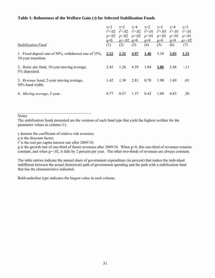
31

Table 1: Robustness of the Welfare Gain () for Selected Stabilization Funds γ=2 γ=2 γ=4 γ=2 γ=2 γ=4 γ=2 rf=.02 rf=.02 rf=.02 rf=.01 rf=.03 rf=.01 rf=.01

ρ=.02 ρ=.02 ρ=.02 ρ=.01 ρ=.03 ρ=.01 ρ=.01 g=0 g=-.02 g=0 g=0 g=0 g=0 g=-.02

Stabilization Fund (1) (2) (3) (4) (5) (6) (7) 1. Fixed deposit rate of 50%, withdrawal rate of 25%, 2.52 2.32 4.97 1.46 3.34 3.03 1.23 10-year transition. 2. Rainy day fund, 10-year moving average, 2.42 1.26 4.59 1.04 3.86 2.48 -.11 5% deposited. 3. Revenue band, 2-year moving average, 1.42 1.30 2.81 0.78 1.98 1.69 .65 50% band width. 4. Moving average, 2-year. 0.77 0.57 1.37 0.42 1.09 0.83 .20 ______________________________________ Notes: The stabilization funds presented are the versions of each fund type that yield the highest welfare for the parameter values in column (1). γ denotes the coefficient of relative risk aversion; ρ is the discount factor; rf is the real per capita interest rate after 2009/10; g is the growth rate of one-third of future revenues after 2009/10. When g=0, this one-third of revenues remains constant, and when g=-.02, it falls by 2 percent per year. The other two-thirds of revenues are always constant. The table entries indicate the annual share of government expenditure (in percent) that makes the individual indifferent between the actual (historical) path of government spending and the path with a stabilization fund that has the characteristics indicated. Bold-underline type indicates the largest value in each column.

32

Table 2: Outcomes for Selected Funds1

Expenditure Expenditure Assets at Assets at Volatility2 Average3 the end of the end of

(percent (percent 2009/104 2009/10 change) difference) (percent (billions)5

difference) Stabilization Fund (1) (2) (3) (4) 1. Fixed deposit of 50%, withdraw 25%, -27.7 1.87 -1.8 22.2 10-year transition. 2. Rainy day fund, 10-year moving -25.0 6.63 -401.3 -68.1 average, 5% deposited in fund. 3. Revenue band, 2-year moving -13.7 0.84 -4.2 21.7 average, 50% band width. 4. Moving average, 2-year. -4.2 1.60 -64.1 8.1 5. Actual data 22.6 ___________________________________________ Notes: Values in columns 1, 2 and 3 are relative to the actual data. 1 None of the values in columns 1 through 4 depend on assumptions with respect to the discount rate, the future interest rate, the coefficient of relative risk aversion, or the path of post-2009/10 income. 2This is the percentage difference from the volatility of the historical path of government spending over the period from 1972/73 - 2009/10. Volatility is measured as the coefficient of variation. 3 Expenditure is average real per capita expenditure relative to the historical average for 1972/73-2009/10. 4 Difference from the assets accumulated given the historical expenditure path for 1972/73-2009/10. 5 Billions of dollars in March 2010 measured in 2010 current dollars.

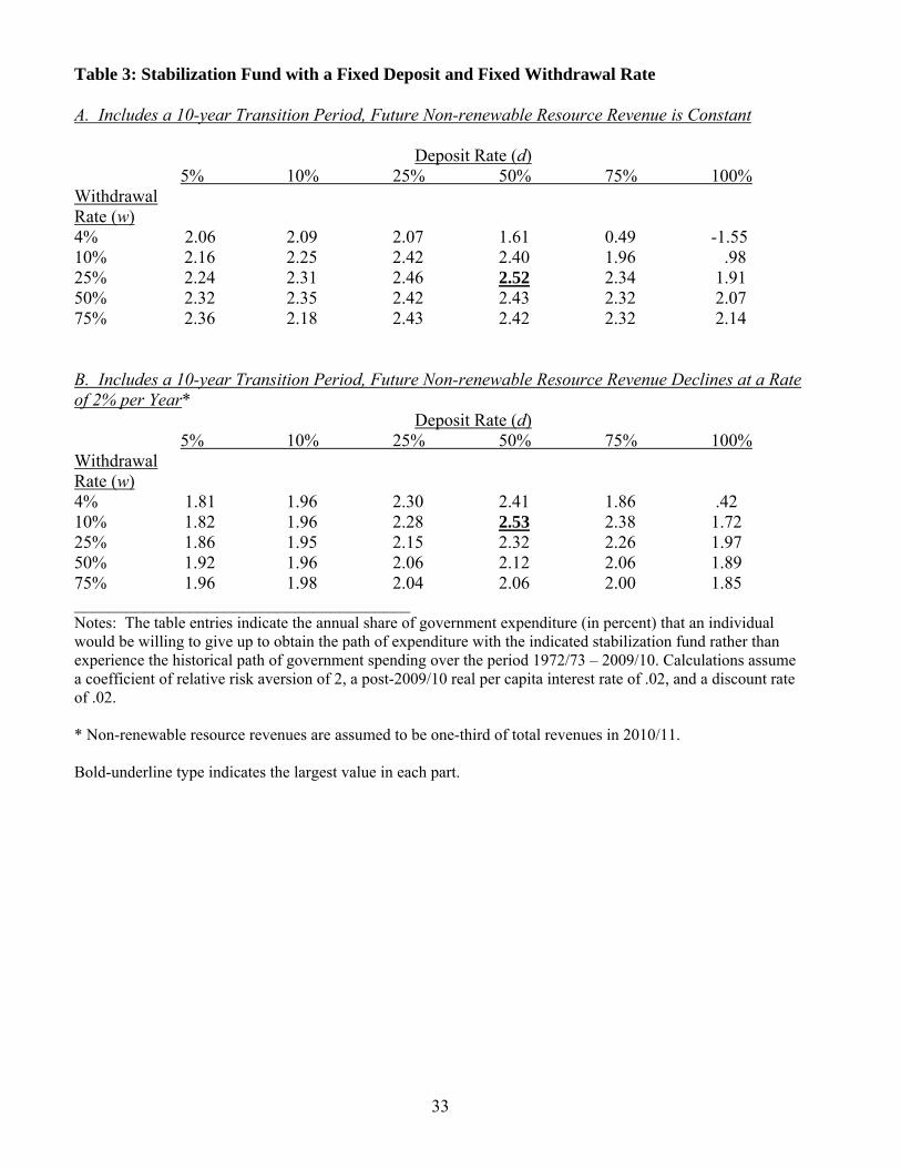
33

Table 3: Stabilization Fund with a Fixed Deposit and Fixed Withdrawal Rate A. Includes a 10-year Transition Period, Future Non-renewable Resource Revenue is Constant Deposit Rate (d) 5% 10% 25% 50% 75% 100% Withdrawal Rate (w) 4% 2.06 2.09 2.07 1.61 0.49 -1.55 10% 2.16 2.25 2.42 2.40 1.96 .98 25% 2.24 2.31 2.46 2.52 2.34 1.91 50% 2.32 2.35 2.42 2.43 2.32 2.07 75% 2.36 2.18 2.43 2.42 2.32 2.14 B. Includes a 10-year Transition Period, Future Non-renewable Resource Revenue Declines at a Rate of 2% per Year* Deposit Rate (d) 5% 10% 25% 50% 75% 100% Withdrawal Rate (w) 4% 1.81 1.96 2.30 2.41 1.86 .42 10% 1.82 1.96 2.28 2.53 2.38 1.72 25% 1.86 1.95 2.15 2.32 2.26 1.97 50% 1.92 1.96 2.06 2.12 2.06 1.89 75% 1.96 1.98 2.04 2.06 2.00 1.85 ______________________________________ Notes: The table entries indicate the annual share of government expenditure (in percent) that an individual would be willing to give up to obtain the path of expenditure with the indicated stabilization fund rather than experience the historical path of government spending over the period 1972/73 – 2009/10. Calculations assume a coefficient of relative risk aversion of 2, a post-2009/10 real per capita interest rate of .02, and a discount rate of .02. * Non-renewable resource revenues are assumed to be one-third of total revenues in 2010/11. Bold-underline type indicates the largest value in each part.

34

Table 4: Robustness of the Welfare Gain () across Deposit and Withdrawal Rates A. Stabilization Fund with a 50% Deposit Rate and Various Fixed Withdrawal Rates, 10-year Transition γ=2 γ=2 γ=4 γ=2 γ=2 γ=4 γ=2 rf=.02 rf=.02 rf=.02 rf=.01 rf=.03 rf=.01 rf=.01

ρ=.02 ρ=.02 ρ=.02 ρ=.01 ρ=.03 ρ=.01 ρ=.01 g=0 g=-.02 g=0 g=0 g=0 g=0 g=-.02 (1) (2) (3) (4) (5) (6) (7)

Withdrawal Rate 4% 1.61 2.41 2.99 1.46 1.30 2.32 2.25 10% 2.40 2.53 4.39 1.62 2.78 2.91 1.71 25% 2.52 2.32 4.97 1.46 3.34 3.03 1.23 50% 2.43 2.12 5.08 1.31 3.44 2.98 .97 75% 2.42 2.06 5.14 1.27 3.49 2.97 .89 B. Stabilization Fund with a 25% Withdrawal Rate and Various Fixed Deposit Rates, 10-year Transition γ=2 γ=2 γ=4 γ=2 γ=2 γ=4 γ=2 rf=.02 rf=.02 rf=.02 rf=.01 rf=.03 rf=.01 rf=.01

ρ=.02 ρ=.02 ρ=.02 ρ=.01 ρ=.03 ρ=.01 ρ=.01 g=0 g=-.02 g=0 g=0 g=0 g=0 g=-.02 (1) (2) (3) (4) (5) (6) (7)

Deposit Rate 5% 2.24 1.86 4.58 1.12 3.34 2.59 .73 10% 2.31 1.95 4.70 1.18 3.39 2.69 .81 25% 2.46 2.15 4.95 1.33 3.46 2.91 1.00 50% 2.52 2.32 4.97 1.46 3.34 3.03 1.23 75% 2.34 2.26 4.51 1.46 2.92 2.86 1.34 100% 1.91 1.97 3.55 1.31 2.17 2.37 1.33 C. Rainy Day Stabilization Fund with Various Fixed Deposit Rates and a 10-year Moving Average Based Expenditure Floor γ=2 γ=2 γ=4 γ=2 γ=2 γ=4 γ=2 rf=.02 rf=.02 rf=.02 rf=.01 rf=.03 rf=.01 rf=.01

ρ=.02 ρ=.02 ρ=.02 ρ=.01 ρ=.03 ρ=.01 ρ=.01 g=0 g=-.02 g=0 g=0 g=0 g=0 g=-.02 (1) (2) (3) (4) (5) (6) (7)

Deposit Rate (1-k) 5% 2.42 1.26 4.59 1.04 3.86 2.48 -.11 10% 2.35 1.61 4.44 1.14 3.52 2.51 .39 15% 2.19 1.85 4.11 1.19 3.04 2.46 .83 20% 1.93 1.98 3.60 1.20 2.43 2.30 1.22 ______________________________________ Notes: γ denotes the coefficient of relative risk aversion; ρ is the discount factor; rf is the real per capita interest rate after 2009/10; g is the growth rate of future real per capita nonrenewable resource income (after 2009/10). When g=0, future nonrenewable natural resource income remains constant, and when g=-.02, these revenues fall by 2 percent per

35

year. Non-renewable resource revenues are assumed to be one-third of total revenues in 2010/11. The table entries indicate the annual share of government expenditure (in percent) that an individual would be willing to give up to obtain the path of expenditure given by the indicated stabilization fund rather than experience the historical path of government spending over the period 1972/73 – 2009/10. Bold-underline type indicates the largest value in each column of each part.

36

Table 5: Rainy Day Fund A. The Future Path of Nonrenewable Natural Resource Revenue is Constant Expenditure floor Percent of Resource Revenues Deposited in the Fund (1-k) based on a 20 15 10 5 moving average of length (years) 2 1.44 1.73 1.93 2.04 3 1.41 1.70 1.90 2.01 5 1.56 1.82 2.00 2.08 7 1.76 2.02 2.18 2.26 10 1.93 2.19 2.35 2.42 B. The Future Path of Nonrenewable Natural Resource Revenue Declines at a rate of 2% Per Year* Expenditure floor Percent of Resource Revenues Deposited in the Fund (1-k) based on a 20 15 10 5 moving average length (years) 2 1.77 1.70 1.54 1.26 3 1.72 1.65 1.48 1.19 5 1.75 1.65 1.44 1.11 7 1.87 1.75 1.52 1.17 10 1.98 1.85 1.61 1.26 ______________________________________ Notes: The table entries indicate the annual share of government expenditure (in percent) that an individual would be willing to give up to obtain the path of expenditure with the indicated stabilization fund rather than experience the historical path of government spending over the period 1972/73 – 2009/10. Calculations assume a coefficient of relative risk aversion of 2, a post-2009/10 real per capita interest rate of .02, and a discount rate of .02. * Non-renewable resource revenues are assumed to be one-third of total revenues in 2010/11. Bold-underline type indicates the largest value in each part.

37