Structured Priors for Multivariate Time Series
20
Journal of Statistical Planning and Inference 136 (2006) 3802 – 3821 www.elsevier.com/locate/jspi Structured priors for multivariate time series Gabriel Huerta a , ∗ , Raquel Prado b a Department of Mathematics and Statistics, University of New Mexico, Albuquerque, NM 87131-1141, USA b Department of Applied Mathematics and Statistics, Baskin School of Engineering, University of California, Santa Cruz 1156 High Street, Santa Cruz, CA 95064, USA Received 13 November 2003; received in revised form 28 February 2005; accepted 28 February 2005 Available online 2 June 2005 Abstract A class of prior distributions for multivariate autoregressive models is presented. This class of priors is built taking into account the latent component structure that characterizes a collection of autoregressive processes. In particular, the state-space representation of a vector autoregressive process leads to the decomposition of each time series in the multivariate process into simple under- lying components. These components may have a common structure across the series. A key feature of the proposed priors is that they allow the modeling of such common structure. This approach also takes into account the uncertainty in the number of latent processes, consequently handling model order uncertainty in the multivariate autoregressive framework. Posterior inference is achieved via standard Markov chain Monte Carlo (MCMC) methods. Issues related to inference and exploration of the posterior distribution are discussed. We illustrate the methodology analyzing two data sets: a synthetic data set with quasi-periodic latent structure, and seasonally adjusted US monthly housing data consisting of housing starts and housing sales over the period 1965 to 1974. © 2005 Elsevier B.V.All rights reserved. MSC: 62H99; 62P20; 62P30 Keywords: Multiple time series; Autoregressions; VAR models; Structured priors; Latent components; Model order uncertainty ∗ Corresponding author. Tel./fax: +1 505 277 2564. E-mail addresses: [email protected] (G. Huerta), [email protected] (R. Prado). 0378-3758/$ - see front matter © 2005 Elsevier B.V. All rights reserved. doi:10.1016/j.jspi.2005.02.025
-
Upload
rokhgirehhojjat -
Category
Documents
-
view
26 -
download
0
description
scientific paper
Transcript of Structured Priors for Multivariate Time Series
Journal of Statistical Planning andInference 136 (2006) 3802–3821
www.elsevier.com/locate/jspi
Structured priors for multivariate time series
Gabriel Huertaa,∗, Raquel Pradob
aDepartment of Mathematics and Statistics, University of New Mexico, Albuquerque, NM 87131-1141, USAbDepartment of Applied Mathematics and Statistics, Baskin School of Engineering, University of California,
Santa Cruz 1156 High Street, Santa Cruz, CA 95064, USA
Received 13 November 2003; received in revised form 28 February 2005; accepted 28 February 2005Available online 2 June 2005
Abstract
A class of prior distributions for multivariate autoregressive models is presented. This class ofpriors is built taking into account the latent component structure that characterizes a collectionof autoregressive processes. In particular, the state-space representation of a vector autoregressiveprocess leads to the decomposition of each time series in the multivariate process into simple under-lying components. These components may have a common structure across the series. A key featureof the proposed priors is that they allow the modeling of such common structure. This approach alsotakes into account the uncertainty in the number of latent processes, consequently handling modelorder uncertainty in the multivariate autoregressive framework. Posterior inference is achieved viastandard Markov chain Monte Carlo (MCMC) methods. Issues related to inference and explorationof the posterior distribution are discussed. We illustrate the methodology analyzing two data sets: asynthetic data set with quasi-periodic latent structure, and seasonally adjusted US monthly housingdata consisting of housing starts and housing sales over the period 1965 to 1974.© 2005 Elsevier B.V. All rights reserved.
MSC: 62H99; 62P20; 62P30
Keywords: Multiple time series; Autoregressions; VAR models; Structured priors; Latent components; Modelorder uncertainty
∗ Corresponding author. Tel./fax: +1 505 277 2564.E-mail addresses: [email protected] (G. Huerta), [email protected] (R. Prado).
0378-3758/$ - see front matter © 2005 Elsevier B.V. All rights reserved.doi:10.1016/j.jspi.2005.02.025
G. Huerta, R. Prado / Journal of Statistical Planning and Inference 136 (2006) 3802–3821 3803
1. Introduction
We propose a class of prior distributions for vector autoregressive processes with diagonalcoefficient matrices or DVAR. The development of these models is motivated by the needof studying multiple series recorded simultaneously in a system under certain conditions.Typically, each one of the multiple time series has an underlying structure, possibly butnot necessarily quasi-periodic, that can be adequately described by an autoregressive (AR)model. Some of the components in this underlying structure are usually shared across themultiple series. Data of this kind arise in many applied areas such as signal processingand econometrics. In particular, univariate time series arising in fields that involve seismicrecordings, environmental time series, biomedical and speech signals, to mention a few,have such characteristics and have been analyzed in the past using autoregressive modelsor sophisticated models that involve autoregressive components. Huerta and West (1999b),Aguilar et al. (1999), Godsill and Rayner (1998), West et al. (1999), Krystal et al. (1999) andKitagawa and Gersch (1996) present examples in the areas of application mentioned above.
A key component of the prior distributions and methods developed here is that they modelthe uncertainty in the number and form of the latent processes related to each univariateseries. In addition, these models provide a way to incorporate prior beliefs on the character-istic roots of the AR processes, including unitary and zero roots. Finally, this methodologyallows the modeler to consider common latent components across the series, which is a veryimportant feature in many applications. For instance, the univariate analyses of several elec-troencephalogram series recorded on a patient under ECT (a treatment of major depression)presented in West et al. (1999) and Krystal et al. (1999) suggest that the multiple series arecharacterized by a common underlying structure with two, or possible three, quasi-periodiccomponents. In this particular application, it is relevant to obtain a probabilistic assessmentof such common latent structure. This can only be done through a multivariate analysis ofthe traces in which the possibly common underlying structure across series is explicitlyincluded in the prior distribution.
Although DVAR models could be perceived as models with very limited practical use,when combined with the structured priors presented here, they form a flexible class of modelsthat can be used to search for latent structure in multiple time series from a multivariateperspective. Therefore, the implementation of DVAR models constitutes a first major steptowards developing more sophisticated multivariate models that can be useful in analyzingvery complex multivariate data, such as the EEG series considered in West et al. (1999) andKrystal et al. (1999).
Priors on latent component structure were introduced for univariate AR models in Huertaand West (1999b). In this sense, the models proposed here are a multivariate extension tothe models developed by Huerta and West. As in the univariate case, posterior inference isachieved via customized MCMC methods. However, additional computational difficultiesarise in the multivariate framework when considering many multiple series with a richlatent component structure. In particular, the exploration of the posterior distribution maybe a difficult task. This is highlighted in one of the examples presented in Section 5. Somealternatives for exploring and summarizing the posterior distribution are investigated.
The paper is organized as follows. Section 2 summarizes the multivariate decompositionresults that motivate the development of the structured priors for DVAR models. Section 3
3804 G. Huerta, R. Prado / Journal of Statistical Planning and Inference 136 (2006) 3802–3821
defines the prior structure in detail and discusses some aspects of assuming such structurewith some examples. Section 4 describes the MCMC methodology to achieve posteriorinference. Section 5 illustrates the methodology with two examples and finally, Section 6presents a discussion and points towards future extensions.
2. Multivariate time series decompositions
In this section, we describe general time series decomposition results for a class ofmultivariate time series processes. The proposed approach focuses on models that can bewritten in a multivariate dynamic linear model (MDLM) form. We discuss such results indetail for the case of diagonal vector autoregressive (DVAR) models. We begin by revisitingthe developments on multivariate time series decompositions presented in Prado (1998),including some extensions that handle more general models.
Consider an m-dimensional time series process yt = (y1,t , . . . , ym,t )′, modeled using a
MDLM (West and Harrison, 1997):
yt = xt + �t , xt = F′�t , �t = Gt�t−1 + �t , (1)
where xt is the underlying m-dimensional signal, �t is an m-dimensional vector of obser-vation errors, F′ is an m × d matrix of constants, �t is the d-dimensional state vector, Gt isthe d × d state evolution matrix and �t is a d-vector of state innovations. The noise terms�t and �t are zero mean innovations, assumed independent and mutually independent withvariance–covariance matrices Vt and Wt , respectively.
A scalar DLM can be written for each of the univariate components of xt as follows:
Mi : xi,t = F′i�t ,
�t = Gt�t−1 + �t ,(2)
with Fi the ith column of the matrix F. We now show that each component xi,t can bewritten as a sum of latent processes using the decomposition results for univariate timeseries presented in West et al. (1999). Assume that the system evolution matrix Gt is diag-onalizable, i.e., that there exist a diagonal matrix At , and a matrix Bt such that Gt =BtAtB
−1t . If Gt has d∗ �d distinct eigenvalues, �t,1, . . . , �t,d∗ with algebraic multiplicities
ma,1, . . . , ma,d∗ respectively, then, Gt is diagonalizable if and only if mg,i = ma,i for alli = 1, . . . , d∗, with mg,i the geometric multiplicity of the eigenvalue �t,i . This is, Gt is di-agonalizable if and only if the algebraic multiplicity of each eigenvalue equals its geometricmultiplicity. In particular, if Gt has exactly d distinct eigenvalues, then Gt is diagonalizable.Note we are assuming that the number of distinct eigenvalues d∗, the number of real andcomplex eigenvalues and their multiplicities remain fixed over time. In other words, weassume that there are exactly c∗ pairs of distinct complex eigenvalues rt,j exp(±i�t,j ) forj =1, . . . , c∗, and r∗=d∗−2c∗ distinct real eigenvalues for j =2c∗+1, . . . , d∗ at each timet. Then, Gt =BtAtB
−1t with At the d×d diagonal matrix of eigenvalues, in arbitrary but fixed
order, and Bt a corresponding matrix of eigenvectors. For each t and each model Mi definethe matrices Hi,t =diag(B′
tFi )B−1t for i=1, . . . , m, and reparameterizeMi via �i,t =Hi,t�t
and �i,t = Hi,t�t . Then, rewriting (2) in terms of the new state and innovation vectors,
G. Huerta, R. Prado / Journal of Statistical Planning and Inference 136 (2006) 3802–3821 3805
we have
xi,t = 1′�i,t ,
�i,t = AtKi,t�i,t−1 + �i,t , (3)
where 1′ = (1, . . . , 1) and Ki,t = Hi,tH−1i,t−1. Therefore xi,t can be expressed as a sum of
d∗ components:
xi,t =c∗∑
j=1
zi,t,j +d∗∑
j=2c∗+1
yi,t,j , (4)
where zi,t,j are real-valued processes related to the pairs of complex eigenvalues given byrt,j exp(±i�t,j ) for j=1, . . . , c∗, and yi,t,j are real processes related to the real eigenvaluesrt,j for j = 2c∗ + 1, . . . , d∗.
2.1. Decomposition of the scalar components in a VARm(p)
Consider the case of an m-dimensional time series process xt that follows a VARm(p):
xt = �1xt−1 + �2xt−1 + · · · + �pxt−p + εt , (5)
where �j for j = 1, . . . , p are the m × m matrices of AR coefficients and εt is the m-dimensional zero mean innovation vector at time t, with covariance matrix �.
Any VARm(p) process can be written in the MDLM form (1), where d = mp, �t = 0; them × (mp) matrix of constants F′ and the (mp)-dimensional state and the state innovationvectors �t and �t are described by
F′ =
⎛⎜⎜⎝
e′1 0 . . . 0
e′2 0 . . . 0...
...
e′m 0 . . . 0
⎞⎟⎟⎠ ; �t =
⎛⎜⎜⎝
xt
xt−1...
xt−p+1
⎞⎟⎟⎠ ; �t =
⎛⎜⎜⎝
εt
0...
0
⎞⎟⎟⎠ . (6)
Here each ej is an m-dimensional vector whose jth element is equal to unity and all theother elements are zeros. Finally, the (mp) × (mp) state evolution matrix G is given by
G =
⎛⎜⎜⎝
�1 �2 . . . �p−1 �p
Im 0m . . . 0m 0m...
. . ....
0m 0m . . . Im 0m
⎞⎟⎟⎠ , (7)
with 0m the m × m dimensional matrix of zeros. The eigenvalues of G satisfy the equation
det(Im�p − �1�p−1 − �2�
p−2 − · · · − �p) = 0,
i.e. they are the reciprocal roots of the characteristic polynomial given by �(u)= det(Im −�1u−· · ·−�pup). Therefore, xt is stable, and consequently stationary, if the eigenvaluesof G have modulus less than one (see for instance Lütkepohl, 1993). Assume that G hasd∗ �mp distinct eigenvalues with c∗ pairs of distinct complex eigenvalues rj exp(±i�j )
3806 G. Huerta, R. Prado / Journal of Statistical Planning and Inference 136 (2006) 3802–3821
for j = 1, . . . , c∗, and r∗ = d∗ − 2c∗ real eigenvalues rj for j = 2c∗ + 1, . . . , d∗. If G isdiagonalizable, then, using (2), (3) and the fact that Ki,t = I for all i, j we have
xi,t =c∗∑
j=1
zi,t,j +d∗∑
j=2c∗+1
yi,t,j . (8)
Now, following the univariate AR decomposition results discussed in West (1997), weobtain that each zi,t,j is a quasi-periodic process following an ARMA(2,1) model withcharacteristic modulus rj and frequency �j for all i = 1, . . . , m. Then, the moduli andfrequencies that characterize the processes zi,t,j for a fixed j are the same across the munivariate series that define the VAR process. Similarly, yi,t,j is an AR(1) process whoseAR coefficient is the real eigenvalue rj for all i = 1, . . . , m.
Example (Vector autoregressions with diagonal matrices of coefficients or DVARm(p)).
Suppose that we have a VARm(p) process with �j =diag(�1,j , . . . ,�m,j ) for j =1, . . . , p.Then, the characteristic polynomial of the process is given by
�(u) =m∏
i=1
(1 − �i,1u − �i,2u2 − · · · − �i,pup) =
m∏i=1
�i (u),
with �i (u) being the characteristic polynomial of series i. In other words, �(u) is theproduct of the characteristic polynomials associated to each of the m series. Let �1
1, . . . , �1p,
. . . , �m1 , . . . , �m
p be the reciprocal roots of the characteristic polynomials �1(u), . . . ,
�m(u), respectively, with �ij �= 0 for all i, j . Assume that for a fixed series i, the re-
ciprocal roots �ij are all distinct, but common roots across series are allowed, i.e., �i
j = �kl
for some i, k such that i �= k and some j, l. If there are c∗ distinct complex pairs of recipro-cal roots, denoted by rj exp(±i�j ) for j = 1, . . . , c∗, r∗ pairs of distinct real roots rj , forj =2c∗ +1, . . . , d∗ with 2c∗ + r∗ =d∗ �mp, and G is diagonalizable, then decomposition(8) holds. We now prove that the state evolution matrix G in this case is diagonalizableby showing that, for any eigenvalue � �= 0 of G, its algebraic multiplicity ma,� equals itsgeometric multiplicity mg,�, with mg,� the dimension of the characteristic subspace of �,{x : (G−�Imp)x=0mp}. Let � be any eigenvalue of G with algebraic multiplicity ma,�. Then,� is either a real or a complex characteristic reciprocal root of �(u), i.e. � = rj exp(i�j ),� = rj exp(−i�j ) or � = rj for some j. The geometric multiplicity of �, mg,�, is the di-mension of the characteristic subspace of �, {x : (G − �Imp)x = 0mp}. The solutions of thesystem (G − �Imp)x = 0, with x = (x1,1, . . . , x1,m, . . . , xp,1, . . . , xp,m) must satisfy the mequations
(�1,1 − �)x1,1 + �1,2x2,1 + · · · + �1,pxp,1 = 0,
�2,1x1,2 + (�2,2 − �)x2,2 + · · · + �2,pxp,2 = 0,
... + . . . + · · · + ......
...
�m,1x1,m + �m,2x2,m + . . . + (�m,p − �)xp,m = 0
G. Huerta, R. Prado / Journal of Statistical Planning and Inference 136 (2006) 3802–3821 3807
and the additional set of mp − m = m(p − 1) equations,
x1,1 − �x2,1 = 0,...
......
......
x1,m − �x2,m = 0,...
......
......
xp−1,1 − �xp,1 = 0,...
......
......
xp−1,m − �xp,m = 0.
Using the last m(p − 1) equations we obtain xi,j = x1,j /�i−1, for i = 2, . . . , p and j =
1, . . . , m. Substituting these expressions in the first m equations we have
x1,j
(1 − �1,j
(1
�
)− �2,j
(1
�
)2
− · · · − �p,j
(1
�
)p)
= 0, j = 1, . . . , m. (9)
Now, � �= 0 has algebraic multiplicity ma,�, therefore, � is a reciprocal root of ma,� charac-teristic polynomials. Let j1, . . . , jma,� be the series associated to such polynomials. Then,Eqs. (9) have non-trivial solutions x1,jk
for k = 1, . . . , ma,� and all the other elements of xcan be written as functions of x1,jk
, k = 1, . . . , ma,�. This implies that mg,� =ma,� for all �and then G is diagonalizable, i.e. G = BAB−1 with A the diagonal matrix of eigenvalues,or reciprocal characteristic roots, and B a corresponding matrix of eigenvectors.
3. The prior structure
We extend the priors on autoregressive root structure developed in Huerta and West(1999b) and studied for spectral estimation in Huerta and West (1999a) to the context ofDVAR models. We also discuss some specific aspects of the prior. In order to keep thenotation as clear as possible, we present the prior distribution for a two-dimensional VARmodel. This structure can be easily generalized for a VARm(p) process.
Assume that we have an m-dimensional series with m = 2. We begin by specifying fixedupper bounds Ci and Ri on the number of complex root pairs and real roots of series i, fori = 1, 2. Conditional on these upper bounds, we assume a prior structure on the componentroots �i
j for j = 1, . . . , 2Ci + Ri , that distinguishes between real and complex cases. Letus introduce some notation that will be useful to define the prior structure.
• rij and �i
j (=2�/�ij ) are the modulus and the wavelength or period of the jth component
root of series i;• �r,−1, �r,0 and �r,1 denote the prior probabilities that a given real root takes the values
−1, 0 and 1, respectively. Similarly, �c,0 and �c,1 denote the prior probabilities that agiven complex root takes the values 0 and 1 respectively.
• �∗r,ri
j
denotes the prior probability that a real root of a series different from i, takes the
value rij conditional on ri
j being different from 0, −1 and 1, and also different from any
3808 G. Huerta, R. Prado / Journal of Statistical Planning and Inference 136 (2006) 3802–3821
of the roots that have already been sampled for such series. This means, “repeated” rootswithin the same series are not permitted. Similarly, �∗
c,rij
denotes the prior probability that
the modulus of a complex root of a series different from i takes the value rij , conditional
on rij being different from 0 and 1 and also different from any of the roots that have
already been sampled for such series.• ri
1:j = {ri1, . . . , r
ij }; �i
1:j = {�i1, . . . , �
ij }; �i
1:j = (r, �)i1:j = {(ri1, �
i1), . . . , (r
ij , �
ij )};• Iy(z) is the indicator function, i.e.,Iy(z) = 1 if z = y and 0 otherwise;
• U(·|a, b) denotes a Uniform distribution over the interval (a, b) and Beta(·|a, b) denotesa Beta distribution with parameters a and b.
We assume the following prior structure on the component roots of the m = 2 series.(a) Priors for real roots. Let R1=2 and R2=2 be the maximum number of real roots of the
first and second series, respectively. Additionally, let rij denote the root j of the series i and
ri1:Ri
all the real roots of series i. A conditional prior structure is proposed: p(r11:R1
, r21:R2
)=p(r1
1:R1)×p(r2
1:R2|r1
1:R1) such that p(r1
1:R1)=∏2
j=1p(r1j ) and p(r2
1:R2|r1
1:R1)=p(r2
1 |r11:R1
)×p(r2
2 |r1:R1 , r21 ). Specifically, we have the following structure for the roots of the first series:
r1j ∼ �r,−1I−1(r
1j ) + �r,0I0(r
1j ) + �r,1I1(r
1j ) + (1 − �r,−1 + �r,0 + �r,1)gr(r
1j ),
for j = 1, 2 and gr(·) is a continuous density over (−1, 1). The mass probability �r,0 is aprior probability at r1
j = 0. This prior probability at zero allows the modeling of uncertaintyin the number of latent components. Additionally, prior point masses at −1 and 1, �r,−1 and�r,1, are incorporated to allow non-stationary components (see Fig. 1). Now, for the rootsof the second series we have
r21 |r1
1 , r12 ∼ �r,−1I−1(r
21 ) + �r,0I0(r
21 ) + �r,1I1(r
21 ) + �∗
r,r11Ir1
1(r2
1 ) + �∗r,r1
2Ir1
2(r2
1 )
+ (1 − �r,−1 − �r,0 − �r,1 − �∗r,r1
1− �∗
r,r12)gr(r
21 ),
r22 |r1
1 , r12 , r2
1 ∼ �r,−1I−1(r22 )+�r,0I0(r
22 )+�r,1I1(r
22 )+�∗
r,r11Ir1
1(r2
2 )+�∗r,r1
2Ir1
2(r2
2 )
+ (1 − �r,−1 −�r,0 −�r,1 −�∗r,r1
1−�∗
r,r12)gr(r
22 ),
where �∗r,r1
j
are prior probabilities on the roots of the first series if such roots are different
from 0, ±1 and have not been sampled already as roots of the second series.Various choices for gr(·) can be considered. For instance, the reference prior is the uni-
form distribution gr(·) = U(·| − 1, 1), i.e., the formal reference prior for the componentAR(1) coefficient ri
j truncated to the stationary region. The prior masses �r,· and �∗r,· can
be considered fixed tuning parameters or alternatively, as it is usually preferred in manyapplications, they can be treated as hyperparameters to be estimated. In the later case rela-tively or absolutely uniform priors that can be viewed as non-informative priors should beimposed on these probabilities. Huerta and West (1999b) propose the use of Dirichlet priordistributions for the univariate case.
G. Huerta, R. Prado / Journal of Statistical Planning and Inference 136 (2006) 3802–3821 3809
-1.0 -0.5 0.0 0.5 1.0
0.0
0.4
0.8
0.0
0.4
0.8
0.0
0.4
0.8
0.0
0.4
0.8
r(1,1)
-1.0 -0.5 0.0 0.5 1.0
r(2,1)
-1.0 -0.5 0.0 0.5 1.0
r(1,2)
-1.0 -0.5 0.0 0.5 1.0
r(2,2)
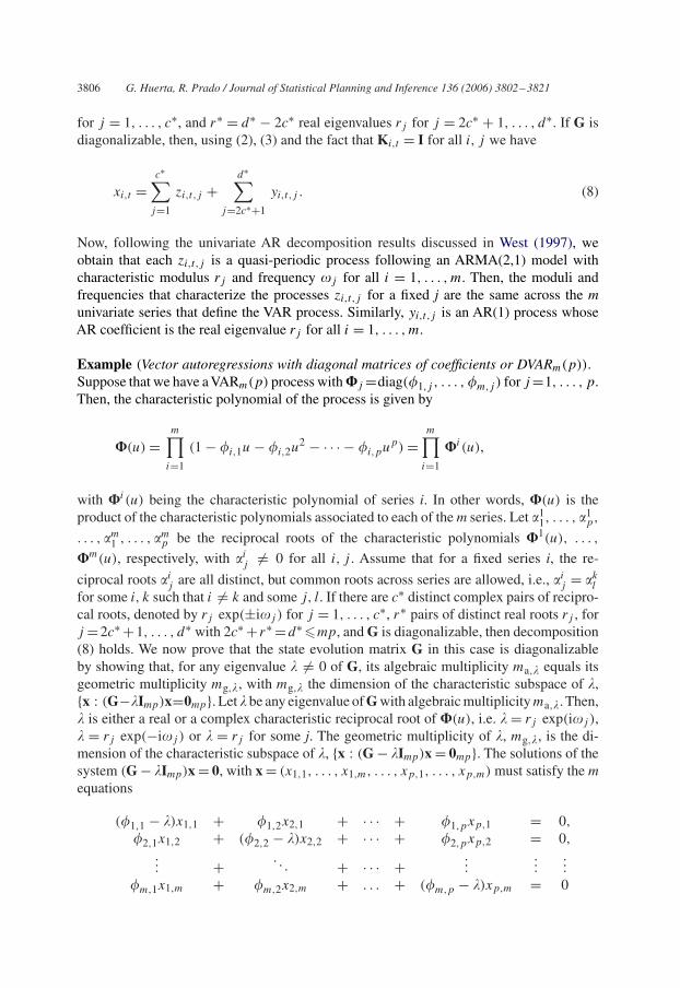
Fig. 1. Prior on real roots. m = 2; R1 = R2 = 2. gr(·) = U(·| − 1, 1). The vertical lines along the (−1, 1) axisrepresent the probability masses for each reciprocal root.
To illustrate the prior on the real reciprocal roots, we use Fig. 1. The first row correspondsto the roots of the first series and the second row, to those of the second series. We areassuming that the continuous part of the prior is U(·| − 1, 1) and the different probabilitymasses are represented by vertical lines. In the figure, we are also including probabilitymasses at the boundary points, −1 and 1. For the roots of the second series, the prior isconditional on r1
1 = −0.65 and r12 = 0.85 and so, point masses appear at these two values.
(b) Priors for complex roots. The structure for the complex roots is similar to that proposedfor the real roots. Again, it is necessary to specify upper bounds for the maximum number ofpairs of complex roots for each series, or equivalently, for the maximum number of quasi-periodic latent processes, and then use a conditional structure. In order to illustrate howthis is done, assume for instance that m = 2 and C1 = C2 = 2 are the maximum number ofpairs of complex roots of the form �i
j = (rij , �
ij ), with ri
j and �ij (=2�/�i
j ), respectively, themodulus and wavelength of the jth quasi-periodic process for series i. Then, a conditionalprior structure p(�1
1:C1, �2
1:C2)=p(�1
1:C1)×p(�2
1:C2|�1
1:C1), is proposed. The component roots
of the first series have an independent prior structure p(�11:C1
)=p(r11 )p(�1
1)p(r12 )p(�1
2) with
priors specified over support 0�r1j �1 and 2 < �1
j < �u for j =1, 2, and a given upper bound�u on the wavelengths. Specifically,
r1j ∼ �c,0I0(r
1j ) + �c,1I1(r
1j ) + (1 − �c,0 − �c,1)gc(r
1j ), �1
j ∼ h(�1j ),
with h(�1j ) a density over the support (2, �u) and gc(·) a continuous density over (0, 1).
Again, �c,0 and �c,1 represent probability masses at values 0 and 1 for the modulus ofthe root. Similar to the real case, the priors on the AR structure for the complex roots ofthe second series, �2
j , are conditional on the root components of the first series and on the
3810 G. Huerta, R. Prado / Journal of Statistical Planning and Inference 136 (2006) 3802–3821
complex roots previously sampled for the second series, i.e.
r21 |r1
1 , r12 ∼ �c,0I0(r
21 ) + �c,1I1(r
21 ) + �∗
c,r11Ir1
1(r2
1 ) + �∗c,r1
2Ir1
2(r2
1 )
+⎛⎝1 − �c,0 − �c,1 −
2∑j=1
�∗c,r1
j
⎞⎠ gc(r
21 ),
r22 |r1
1 , r12 , r2
1 ∼ �c,0I0(r22 ) + �c,1I1(r
22 ) + �∗
c,r11Ir1
1(r2
2 ) + �∗c,r1
2Ir1
2(r2
2 )
+⎛⎝1 − �c,0 − �c,1 −
2∑j=1
�∗c,r1
j
⎞⎠ gc(r
22 ),
�21|�1
1, �12 ∼
2∑j=1
Ir1j(r2
j )I�1j(�2
1) +⎡⎣1 −
2∑j=1
Ir1j(r2
j )I�1j(�2
1)
⎤⎦h(�2
1),
�22|�1
1, �12, �
21 ∼
2∑j=1
Ir1j(r2
j )I�1j(�2
2) +⎡⎣1 −
2∑j=1
Ir1j(r2
j )I�1j(�2
2)
⎤⎦h(�2
2).
Different choices for gc(rij ) and h(�i
j ) can be considered, including uniform priors and
marginals for �ij based on uniform priors for the corresponding frequency �i
j . The defaultprior is the “component reference prior” (Huerta and West, 1999b), induced by assuming auniform prior for the implied AR(2) coefficients 2ri
j cos(2�/�ij ) and −(ri
j )2, but with finite
support for �ij . In addition, as with the real roots, relatively or absolutely continuous priors
can be imposed on �c,· and �∗c,·.
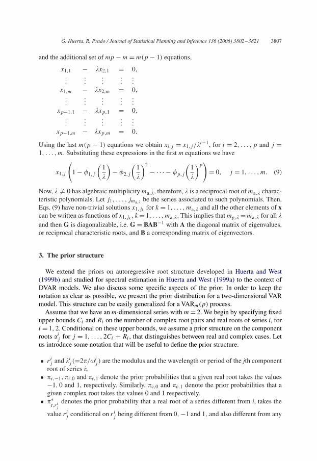
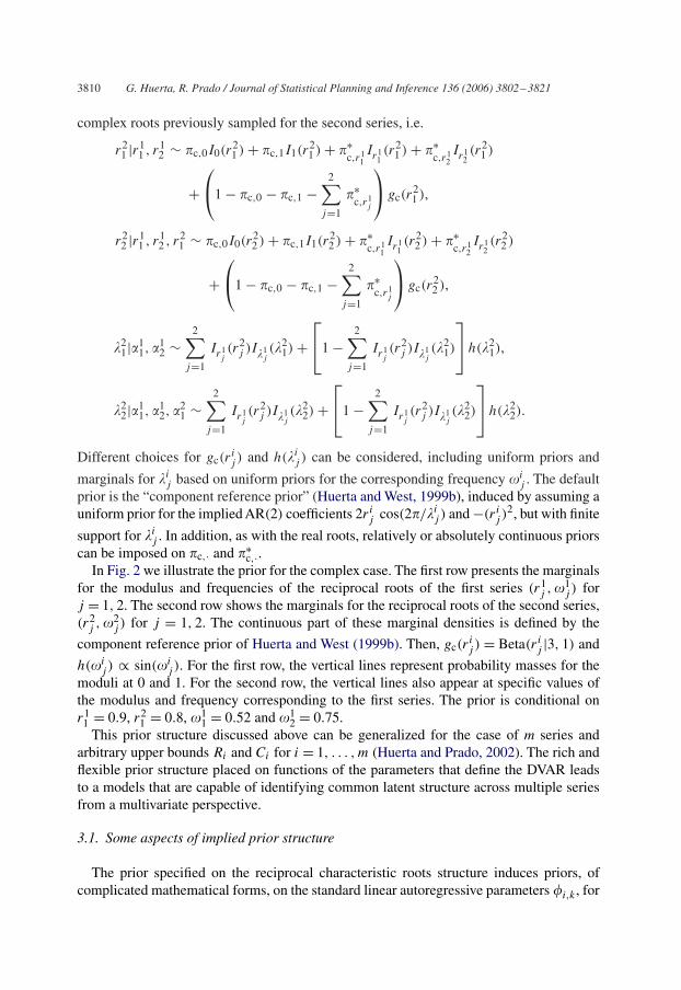
In Fig. 2 we illustrate the prior for the complex case. The first row presents the marginalsfor the modulus and frequencies of the reciprocal roots of the first series (r1
j , �1j ) for
j = 1, 2. The second row shows the marginals for the reciprocal roots of the second series,(r2
j , �2j ) for j = 1, 2. The continuous part of these marginal densities is defined by the
component reference prior of Huerta and West (1999b). Then, gc(rij ) = Beta(ri
j |3, 1) and
h(�ij ) ∝ sin(�i
j ). For the first row, the vertical lines represent probability masses for themoduli at 0 and 1. For the second row, the vertical lines also appear at specific values ofthe modulus and frequency corresponding to the first series. The prior is conditional onr1
1 = 0.9, r21 = 0.8, �1
1 = 0.52 and �12 = 0.75.
This prior structure discussed above can be generalized for the case of m series andarbitrary upper bounds Ri and Ci for i = 1, . . . , m (Huerta and Prado, 2002). The rich andflexible prior structure placed on functions of the parameters that define the DVAR leadsto a models that are capable of identifying common latent structure across multiple seriesfrom a multivariate perspective.
3.1. Some aspects of implied prior structure
The prior specified on the reciprocal characteristic roots structure induces priors, ofcomplicated mathematical forms, on the standard linear autoregressive parameters �i,k , for
G. Huerta, R. Prado / Journal of Statistical Planning and Inference 136 (2006) 3802–3821 3811
0.0 0.4 0.8
0.0
1.0
2.0
3.0
0.0
1.0
2.0
3.0
r(1,1)
0.0 1.5 3.0
0.0
0.4
0.8
0.0
0.4
0.8
w(1,1)
0.0 0.4 0.8
0.0
1.0
2.0
3.0
0.0
1.0
2.0
3.0
r(2,1)
0.0 1.5 3.0
0.0
0.4
0.8
w(2,1)
0.0 0.4 0.8
r(1,2)
0.0 1.5 3.0
w(1,2)
0.0 0.4 0.8
r(2,2)
0.0 1.5 3.0
0.0
0.4
0.8
w(2,2)
Fig. 2. Prior on complex roots m = 2; C1 = C2 = 2; gc(·) and h(·) are specified with the component referenceprior. The figure shows the marginals for ri
jand �i
j. The vertical lines indicate a probability mass.
i = 1, . . . , m and k = 1, . . . , p. For instance, consider a VAR2(5) model that allows exactlyone real component in each series R1 = R2 = 1, and two quasi-periodic components ineach series, C1 = C2 = 2. Some of the point masses are set to zero by making �r1,0 =�r2,0 = �c1,0 = �c2,0 = 0, �r1,−1 = �r2,−1 = 0 and �r1,1 = �r2,1 = �c1,1 = �c2,1 = 0. Inaddition, we take gr(r
ij ), gc(r
ij ) and h(�i
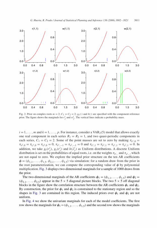
j ) as Uniform distributions. A discrete Uniformdistribution is set on the probabilities of equal roots, i.e. on the weights �ri ,· and �ci ,·, whichare not equal to zero. We explore the implied prior structure on the ten AR coefficients� = (�1,1, . . . ,�1,5, �2,1, . . . ,�2,5) via simulation: for a random draw from the prior inthe root parameterization, we can compute the corresponding value of � by polynomialmultiplication. Fig. 3 displays two-dimensional marginals for a sample of 1000 draws fromthe prior.
The two-dimensional marginals of the AR coefficients �1 = (�1,1, . . . ,�1,5) and �2 =(�2,1, . . . ,�2,5) appear in the 5 × 5 diagonal picture blocks. The two 5 × 5 off diagonalblocks in the figure show the correlation structure between the AR coefficients �1 and �2.By construction, the prior for �1 and �2 is constrained to the stationary region and so theshapes in Fig. 3 are contained in this region. The induced priors over �1 and �2 are notuniform.
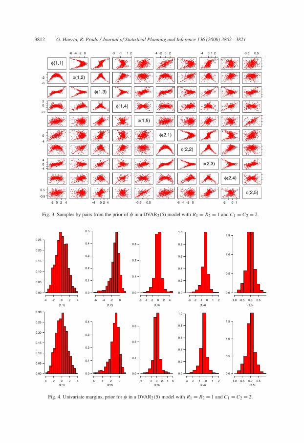
In Fig. 4 we show the univariate marginals for each of the model coefficients. The firstrow shows the marginals for �1 = (�1,1, . . . ,�1,5) and the second row shows the marginals
3812 G. Huerta, R. Prado / Journal of Statistical Planning and Inference 136 (2006) 3802–3821
φ(1,1)
-6 -4 -2 0 -3 -1 1 2 -4 -2 0 2 -4 0 1 2 -0.5 0.5
-6
-2 φ(1,2)
φ(1,3)
-3
0 φ(1,4)
φ(1,5)
-4
0 φ(2,1)
φ(2,2)
-40 φ(2,3)
φ(2,4)
-2 0 2 4
-0.5
0.5
-4 0 2 4 -0.5 0.5 -6 -4 -2 0 -2 0 1
φ(2,5)
4
2
Fig. 3. Samples by pairs from the prior of � in a DVAR2(5) model with R1 = R2 = 1 and C1 = C2 = 2.
(1,1)
-4 -2 0 2 4
0.00
0.05
0.10
0.15
0.20
0.25
(1,2)
-6 -4 -2 0
0.0
0.1
0.2
0.3
0.4
0.5
(1,3)
-6 -4 -2 0 2 4
0.0
0.1
0.2
0.3
(1,4)
-3 -2 -1 0 1 2
0.0
0.2
0.4
0.6
0.8
1.0
(1,5)
-1.0 -0.5 0.0 0.5
0.0
0.5
1.0
1.5
(2,1)
-4 -2 0 2 4
0.00
0.05
0.10
0.15
0.20
0.25
0.30
(2,2)
-6 -4 -2 0
0.0
0.1
0.2
0.3
0.4
(2,3)
- 6 -2 0
0.0
0.1
0.2
0.3
(2,4)
-3 -2 -1 0 1 2
0.0
0.2
0.4
0.6
0.8
1.0
(2,5)
-1.0 -0.5 0.0 0.5
0.0
0.5
1.0
1.5
2 4 6
Fig. 4. Univariate margins, prior for � in a DVAR2(5) model with R1 = R2 = 1 and C1 = C2 = 2.
G. Huerta, R. Prado / Journal of Statistical Planning and Inference 136 (2006) 3802–3821 3813
for �2 = (�2,1, . . . ,�2,5). This is a shrinkage prior in the sense that as the lag of the ARcoefficient increases, the prior mass is more concentrated around zero. The marginal priordistribution for each AR coefficient is, in general, not symmetric.
4. Posterior structure in DVAR models
Posterior and predictive calculations are obtained via Markov chain Monte Carlo (MCMC)simulation methods. We briefly outline the structure of relevant conditional posterior dis-tributions.
Assume we have m series. Let X = {x1, . . . , xn}, with xt = (x1,t , . . . , xm,t )′, be the
observed m-dimensional time series vector. Given the maximum model order p, withp = max{p1, . . . , pm}, write X0 = {x0, x−1, . . . , x−(p−1)} for the latent initial values.Let � be the m × m variance–covariance matrix. The model parameters are denoted by� = {�1
1, . . . , �1p1
, . . . , �m1 , . . . , �m
pm}. Assuming that � and X0 are known, the posterior in-
ferences are based on summarizing the full posterior p(�|X0, X, �). For any subset ofelements of �, let �\ denote the elements of � with removed. The MCMC method usedto obtain samples from the posterior distribution follows a standard Gibbs sampling format,specifically
• for each i = 1, . . . , m,
1. sample the real roots individually from p(rij |�\ri
j , X, X0, �), for eachj = 2Ci +1, . . . , 2Ci + Ri ;
2. sample the complex roots individually from p(�ij |�\�i
j , X, X0, �), for each j =1, . . . , Ci .
Specific details about how to sample from the distributions in steps 1 and 2 of the MCMCalgorithm are given below.
1. Conditional distributions for real roots. Assume that we want to obtain a sample fromthe conditional distribution p(ri
j |�\rij , X, X0, �), for some series i and some j. Given all the
other model parameters and the DVAR structure, the likelihood function for rij provides a
normal kernel. Therefore, under a mixture prior of the form previously described in Section5, this leads to the mixture posterior
i−1∑l=1
Rl∑k=1
pi
j,rlk
Irlk(ri
j ) +∑
q=−1,0,1
pj,qIq(rij )
+⎛⎝1 −
∑q=−1,0,1
pj,q −i−1∑l=1
Rl∑k=1
pi
j,rlk
⎞⎠Nt(r
ij |mi
j , Mij ).
Here Nt(·|m, M) denotes the density of a normal distribution with mean m and variance Mtruncated to (−1, 1). The values (mi
j , Mij ) and the point masses can be easily computed.
This mixture posterior is easily sampled with direct simulation of the truncated normal byc.d.f. inversion.
3814 G. Huerta, R. Prado / Journal of Statistical Planning and Inference 136 (2006) 3802–3821
2. Conditional for complex roots. For each series i, the index j, with j = 1, . . . , Ci ,identifies a pair of complex conjugate roots (�i
2j−1, �i2j ) with parameters (ri
j , �ij ). Let Ai
j
be the index set of all other roots, �\(rij , �
ij ). Given �\(ri
j , �ij ) and X we can directly compute
the filtered time series as zt,l =∏k∈Aij(1−�l
kB)xt,l if l= i and zt,l =∏pl
k=1(1−�ijB)xt,l for
l �= j . Now, the likelihood on �ij,1 =2ri
j cos(2�/�ij ) and �i
j,2 =−(rij )
2 provides a bivariatenormal kernel with a mean vector and a variance–covariance matrix that are functions ofthe filtered time series zt,1, . . . , zt,m. However, given that the support of (�i
j,1, �ij,2) is
a bounded region defined by the stationary condition of the process, sampling from theresulting conditional posterior directly is difficult. Because of this and following Huertaand West (1999b), we use a reversible jump Markov chain Monte Carlo step.
The structure of the MCMC algorithm in the multivariate case is very similar to thestructure of the MCMC algorithm developed in Huerta and West (1999b) for the univariatecase. However, the number of computations increases considerably when the number ofseries and/or the model orders are large. This issue will be addressed in the followingexamples.
5. Examples
5.1. Analysis of synthetic data
Fig. 5 displays two time series of 500 observations simulated with innovation covariancematrix � = 10.0 ∗ I3 and the following latent structure. The first series was generated froman AR process with one real root with modulus r1
1 = 0.98 and two pairs of complex rootswith modulus and wavelengths of r1
2 = 0.97, r13 = 0.8 and �1
2 = 17.0, �13 = 6.0, respectively.
The second series has one common pair of roots with the first series, namely r22 = 0.97
0 100 200 300 400 500
-500
-200
0
200
time(a)
0 100 200 300 400 500
-20
0
10
20
time(b)
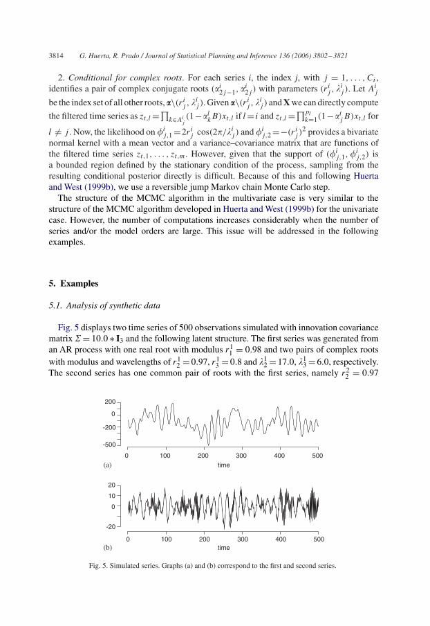
Fig. 5. Simulated series. Graphs (a) and (b) correspond to the first and second series.
G. Huerta, R. Prado / Journal of Statistical Planning and Inference 136 (2006) 3802–3821 3815
and �22 =17.0, another pair characterized by r2
3 =0.8 and �23 =3.0 and a real root r2
1 =−0.98.Parameter estimation using a prior structure with a maximum of three pairs of complex rootsCi=3 and one real root Ri=1 per series is achieved via the reversible jump MCMC algorithmdetailed in the previous section. The prior masses for the roots on the stationary boundarywere set to zero. Discrete uniform priors were used for the prior masses of the roots lying inthe stationary region. In addition, gr(·), gc(·) and h(·) were taken as component referencepriors. The results presented here are based on 4000 samples from the posterior distributiontaken after convergence was achieved, following a burn-in period of 10,000 iterations.
Exploring the posterior distribution involves thinking about the possible models thatmay result from considering the priors described in Section 3. We use a vectorial notationto denote the structure of a given model. For instance, in this example, a possible modelstructure is (R1
1, 0, C12 , C1
3 ; 0, C12 , C2
2 , C23 ). In this notation the first four components of
the vector refer to the roots of the first series, while the last four refer to the roots of thesecond series. This is, for the first series, the first root is a real root different from zero, thesecond root is a zero root and the third and fourth roots are complex and different from zero.Similarly, for the second series, the first root is a zero root, the second one is a complex rootequal to the third root of the first series and the third and fourth components are complexroots different from zero and also different from any of the complex roots of first series.Note that in this example the number of possible models is large, considering that we havea small number of series (m = 2) and relatively small model orders (the maximum modelorder per series is 7). For a single time series with a maximum of one real root and threecomplex roots, we have a total number of 8 possible models. When a second series withsimilar structure is added, the number of possible models increases enormously due to thefact that the roots of the first series can also appear in the second series if common latentstructure is shared by the two series. For instance, considering only the models in whichall the roots are distinct, or in which only the real root can be repeated and all the complexroots are distinct, we get 80 models. It is easy to see that the total number of models thatcan be considered in cases where several series with a rich latent component structure haveto be analyzed is very large.
One possible way to explore the posterior distribution is by looking at the resultsmarginally. In this example we obtain that the terms with the highest marginal posteri-ors and their corresponding probabilities are
Pr(R11 ∼ R|X) = 1.000, Pr(C1
1 = 0|X) = 0.721,
Pr(C12 ∼ C|X) = 1.000, Pr(C1
3 ∼ C|X) = 1.000,
for the first series and
Pr(R21 ∼ R|X) = 1.000, Pr(C2
1 = 0|X) = 0.826,
Pr(C22 = C1
2 |X) = 0.526, Pr(C23 ∼ C|X) = 0.710,
for the second series. Therefore, if we have to select a model structure based on thesemarginal posterior results we would choose model M : (R1
1, 0, C12 , C1
3 ; R21, 0, C1
2 , C23 ).
Then, according to model M, the first series is characterized by one real root, a zero rootand two complex roots, while the second series has a real root, a zero root and two complexroots, one of which is a repeated root from the first series.
3816 G. Huerta, R. Prado / Journal of Statistical Planning and Inference 136 (2006) 3802–3821
r(1,1)0.88 0.90 0.92 0.94 0.96 0.98 1.00
0
100
300
r(1,2)-1.00 -0.95 -0.90 -0.85 -0.80
0
200
600
(a)
(b)
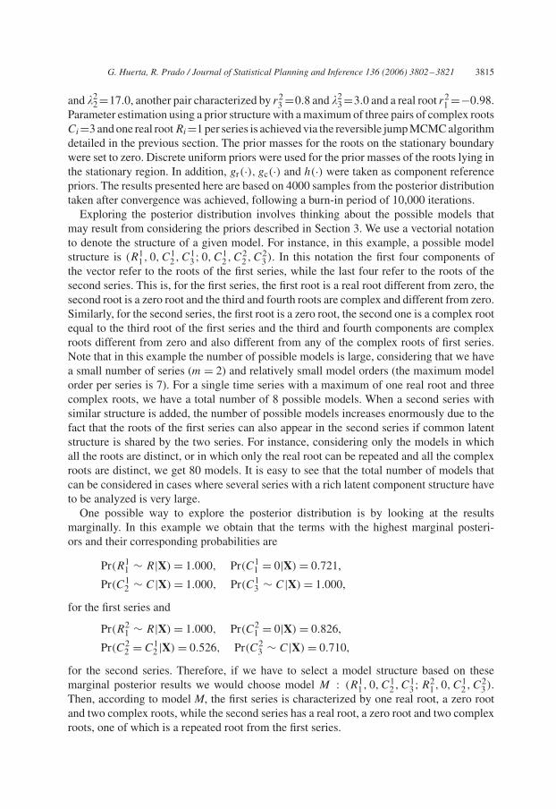
Fig. 6. Graphs (a) and (b) display the posteriors of the two real roots for the simulated series.
In this example, the model built from the terms with the highest marginal posteriors isthe correct model, since it captures the structure used to simulate the two series. However,this is not necessarily the case in all the applications (see Huerta and Prado, 2002) and so, itis important to look for the model with the highest joint posterior probability. A good wayof finding models with high joint posterior probabilities is by means of clustering analysis,following an idea proposed in Bielza et al. (1996) and used in Sansó and Müller (1997) inthe context of optimal design problems. If a distance between models is defined, then it ispossible to produce a cluster tree, cut the tree of model structures at a certain height andconsider the sizes and the models of the resulting cluster. In this case it was possible tofollow this idea, cut the tree at zero height, since various models were visited several times,and find the cluster with the largest size. The following three models were the most likelymodels obtained after exploring the joint posterior distribution
Pr(R11, 0, C1
2 , C13 ; R2
1, 0, C12 , C2
3 ) = 0.377,
Pr(R11, C1
1 , C12 , C1
3 ; R21, 0, C1
2 , C23 ) = 0.192,
Pr(R11, 0, C1
2 , C13 ; R2
1, 0, 0, C23 ) = 0.092.
Again, the most popular model was the correct model M : (R11, 0, C1
2 , C13 ; R2
1, 0, C12 , C2
3 )
with posterior probability 0.38.Fig. 6 shows the histogram of the posterior samples of the real root for the first series (graph
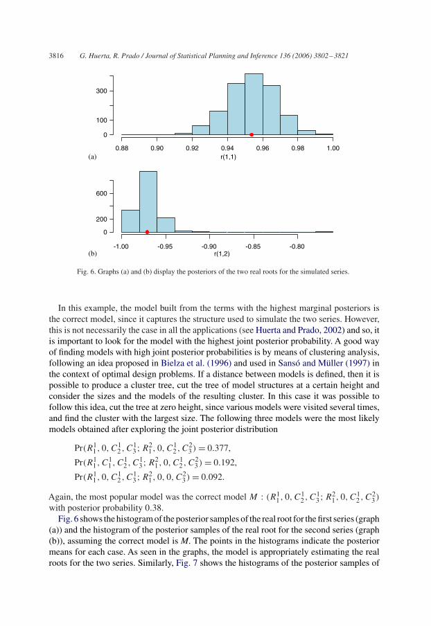
(a)) and the histogram of the posterior samples of the real root for the second series (graph(b)), assuming the correct model is M. The points in the histograms indicate the posteriormeans for each case. As seen in the graphs, the model is appropriately estimating the realroots for the two series. Similarly, Fig. 7 shows the histograms of the posterior samples of
G. Huerta, R. Prado / Journal of Statistical Planning and Inference 136 (2006) 3802–3821 3817
r(2,1)0.94 0.96 0.98
0
100
200
300
r(3,1)0.75 0.80 0.85
0
50
100
150
200
250
r(3,2)0.2 0.4 0.6 0.8
0
200
400
600
800
1000
lambda(2,1)16.5 17.5 18.5
0
50
100
150
200
250
300
lambda(3,1)5.4 5.6 5.8 6.0 6.2 6.4
0
100
200
300
400
lambda(3,2)3.0 3.5 4.0 4.5
0
200
400
600
800
1000
1200
(a)
(d)
(b) (c)
(f)(e)
Fig. 7. Graphs (a)–(f) display the posteriors for the complex roots of the two simulated series.
the complex roots for the first and second series. In these graphs we are conditioning on themodel structure M. Then, panels (a) and (d) display, respectively, the posterior distributionsof the modulus and wavelength of the complex root with the highest modulus for the firstand second series. Panels (b) and (e) show the modulus and wavelength of the complex rootwith the smallest modulus for the first series. Finally, panels (c) and (f) show the modulusand wavelength of the complex root with the smallest modulus for the second series. Asseen in these graphs, our methodology performs very well in terms of capturing the latentstructure present in the simulated data.
The results and figures presented so far are conditional results, i.e., we are looking atthe posterior distribution for the parameters conditioning on M, the model with the highestposterior probability, being the correct model. It is also possible to report some interestingresults obtained by averaging across all possible models. For example, the posterior prob-ability that the two series have real roots different from zero is one: Pr(R1
1 �= 0 & R12 �=
3818 G. Huerta, R. Prado / Journal of Statistical Planning and Inference 136 (2006) 3802–3821
Housing Starts Series
r(1,1)
-0.6 -0.5 -0.4 -0.3 -0.2 -0.1 0.0
0
1
2
3
4
Housing Starts Series
r(2,1)
0.85 0.90 0.95 1.00
0
20
40
60
80
Houses Sold Series
r(1,2)
-0.6 -0.4 -0.2 0.0
0
1
2
3
4
Houses Sold Series
r(2,2)
0.85 0.90 0.95 1.00
0
20
40
60
80
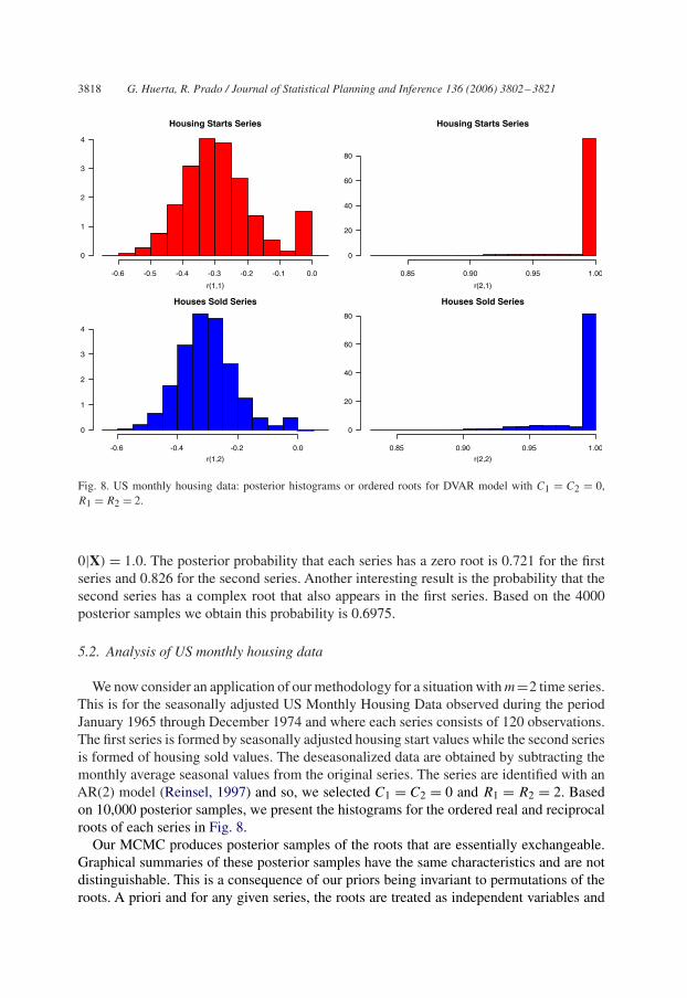
Fig. 8. US monthly housing data: posterior histograms or ordered roots for DVAR model with C1 = C2 = 0,R1 = R2 = 2.
0|X) = 1.0. The posterior probability that each series has a zero root is 0.721 for the firstseries and 0.826 for the second series. Another interesting result is the probability that thesecond series has a complex root that also appears in the first series. Based on the 4000posterior samples we obtain this probability is 0.6975.
5.2. Analysis of US monthly housing data
We now consider an application of our methodology for a situation with m=2 time series.This is for the seasonally adjusted US Monthly Housing Data observed during the periodJanuary 1965 through December 1974 and where each series consists of 120 observations.The first series is formed by seasonally adjusted housing start values while the second seriesis formed of housing sold values. The deseasonalized data are obtained by subtracting themonthly average seasonal values from the original series. The series are identified with anAR(2) model (Reinsel, 1997) and so, we selected C1 = C2 = 0 and R1 = R2 = 2. Basedon 10,000 posterior samples, we present the histograms for the ordered real and reciprocalroots of each series in Fig. 8.
Our MCMC produces posterior samples of the roots that are essentially exchangeable.Graphical summaries of these posterior samples have the same characteristics and are notdistinguishable. This is a consequence of our priors being invariant to permutations of theroots. A priori and for any given series, the roots are treated as independent variables and
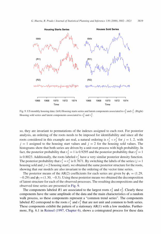
G. Huerta, R. Prado / Journal of Statistical Planning and Inference 136 (2006) 3802–3821 3819
Housing Starts Series
Time
data
(R1)
(R2)
1966 1968 1970 1972 1974
Houses Sold Series
Time
data
(R1)
(R2)
1966 1968 1970 1972 1974
Fig. 9. US monthly housing data: (left) Housing starts series and latent components associated to r22 and r1
1 . (Right)
Housing sold series and latent components associated to r22 and r2
1 .
so, they are invariant to permutations of the indexes assigned to each root. For posterioranalysis, an ordering of the roots needs to be imposed for identifiability and since all theroots considered in this example are real, a natural ordering is r
j1 < r
j2 for j = 1, 2, with
j = 1 assigned to the housing start values and j = 2 for the housing sold values. Thehistograms show that both series are driven by a unit root process with high probability. Infact, the posterior probability that r1
2 = 1 is 0.9295 and the posterior probability that r22 = 1
is 0.8023. Additionally, the roots labeled rj1 have a very similar posterior density function.
The posterior probability that r11 = r2
1 is 0.7671. By switching the labels of the series (j = 1housing sold and j =2 housing start), we obtained the same posterior structure for the roots,showing that our models are also invariant to the ordering of the vector time series.
The posterior means of the AR(2) coefficients for each series are given by �1 = (1.29,
−0.29) and �2 =(1.30, −0.3). Using these posterior means we obtained the decompositionof latent structure for each of the observed processes. The resulting decompositions and theobserved time series are presented in Fig. 9.
The components labeled R1 are associated to the largest roots r12 and r2
2 . Clearly thesecomponents have the same amplitude of the data and the main characteristics of a randomwalk process, so these components represent a “common trend series”. The componentslabeled R2 correspond to the roots r1
1 and r21 that are not unit and common to both series.
These components exhibit the pattern of a stationary AR(1) with a low modulus. Further-more, Fig. 6.1 in Reinsel (1997, Chapter 6), shows a cointegrated process for these data
3820 G. Huerta, R. Prado / Journal of Statistical Planning and Inference 136 (2006) 3802–3821
using a VAR2(1) formulated via canonical correlations. Our components labeled R2 resem-ble the transformed series by Reinsel and correspond to the stationary latent componentunderlying the two series.
6. Conclusions and extensions
A new class of prior distributions for multivariate times series models that follow a vectorautoregressive structure with diagonal coefficient matrices is presented here. This class ofpriors naturally incorporates model order uncertainty and characteristic root structure in amultivariate framework.
Vector autoregressions with upper triangular or lower triangular matrices of coefficients,as the DVAR models, have characteristic polynomials that can be written as the product ofpolynomials associated with each individual series. In future research we will investigate theuse of structured priors for triangular VAR models. It is natural to use the priors developedhere for the coefficients that lie on the diagonal of the triangular VAR coefficient matrices,since these parameters define the latent structure of the individual series. In addition, avariety of priors can be considered for the coefficients that lie off the diagonal in triangularVAR processes. Such coefficients model the dependence of one particular series and thelagged values of the rest of the series. So a prior structure with spikes at zero could beused to allow the inclusion or exclusion of such coefficients. If a coefficient is included, acontinuous prior can be specified.
For general VAR processes with coefficient matrices �j of arbitrary form, it is not trivialto extend the prior structure developed in Section 3. In particular, extending such priorstructure in a way that guarantees stationarity of the VAR process is a very difficult task.The latent processes of each of the scalar components in the multivariate series are defined interms of the roots of the characteristic polynomial, which for general VAR processes cannotbe written as the product of individual characteristic polynomials. In connection with this,transformations of the VAR leading to a collection of univariate processes that can be fittedseparately, such as the transformations proposed by Kitagawa and Gersch (1996), will beconsidered in future extensions of this work.
One of the assumptions made here was that of the innovation error covariance matrix �is known. This assumption can be relaxed with the use of inverse-Wishart priors. Alterna-tively, representations of � where the matrix elements take simple parametric forms suchas �2�|i−j |, lead to prior specifications of only a few parameters. Reference priors as inYang and Berger (1994) and the conditionally conjugate prior distributions for covariancematrices presented in Daniels and Pourahmadi (2002) can also be explored.
Finally, the proposed structured prior leads to exploration of a very large model spacethrough MCMC simulation. The use of clustering ideas for more efficient exploration ofthe posterior distributions of interest is initially investigated here. We expect to furtherinvestigate this issue by defining distances between models. Such distances can be definedin terms of the closeness of the latent structures of the different models considered. Modelswith different structures which may be roughly equivalent in terms of the dominant latentcomponents, or equivalent in terms of predictive performance, would belong to the sameclass of models. The classes can be defined in terms of a given distance. Then, it would be
G. Huerta, R. Prado / Journal of Statistical Planning and Inference 136 (2006) 3802–3821 3821
possible to, for example, choose the most parsimonious model within a particular class inorder to describe the structure of the series or for predictive purposes.
Acknowledgements
We wish to express our gratitude to the Associate Editor and to the referee for theircomments on a previous version of this paper.
References
Aguilar, O., Huerta, G., Prado, R., West, M., 1999. Bayesian inference on latent structure in time series (withdiscussion). In: Bernardo, J.M., et al. (Eds.), Bayesian Statistics 6. pp. 3–26.
Bielza, C., Müller, P., Ríos-Insúa, D., 1996. Monte Carlo methods for decision analysis with applications toinfluence diagrams. Technical Report 96-07. ISDS, Duke University, 1996.
Daniels, M.J., Pourahmadi, M., 2002. Bayesian analysis of covariance matrices and dynamic models forlongitudinal data. Biometrika 89, 553–566.
Godsill, S.J., Rayner, P.J.W., 1998. Digital Audio Restoration: A Statistical Model-Based Approach. Springer,Berlin.
Huerta, G., Prado, R., 2002. Exploring common structure in multiple time series via structured priors forautoregressive processes. Technical Report. AMS, UC Santa Cruz and Department of Mathematics andStatistics, University of New Mexico, 2002.
Huerta, G., West, M., 1999a. Bayesian inference on periodicities and component spectral structure in time series.J. Time Series Anal. 20, 401–416.
Huerta, G., West, M., 1999b. Priors and component structures in autoregressive time series models. J. R. Statist.Soc. B. 61, 881–899.
Kitagawa, G., Gersch, W. 1996. Smoothness Priors Analysis of Time Series, Lecture Notes in Statistics, vol. 116.Springer, New York.
Krystal, A.D., Prado, R., West, M., 1999. New methods of time series analysis of non-stationary EEG data:eigenstructure decompositions of time-varying autoregressions. Clin. Neurophysiol. 110, 2197–2206.
Lütkepohl, H., 1993. Introduction to Multiple Time Series Analysis. second ed. Springer, Heidelberg.Prado, R. 1998. Latent structure in non-stationary time series. Ph.D. Thesis, Duke University, Durham, NC.Reinsel, G.C., 1997. Elements of Multivariate Time Series Analysis. second ed. Springer, New York.Sansó, B., Müller, P. 1997. Redesigning a network of rainfall stations. In: Case Studies in Bayesian Statistics, vol.
IV. Springer, New York, pp. 383–394.West, M., 1997. Time series decomposition. Biometrika 84, 489–494.West, M., Harrison, J., 1997. Bayesian Forecasting and Dynamic Models. second ed. Springer, New York.West, M., Prado, R., Krystal, A.D., 1999. Evaluation and comparison of EEG traces: Latent structure in
nonstationary time series. J. Amer. Statist. Assoc. 94, 1083–1095.Yang, R., Berger, J., 1994. Estimation of a covariance matrix using the reference prior. Ann. Statist. 22, 1195–
1211.