Structure Learning Colocation Patterns
51
“Strategy is the art of making use of time and space. I am less concerned about the latter than the former.” “Space we can recover, lost time never.” – Napoleon Bonaparte
-
Upload
james-matthew-miraflor -
Category
Data & Analytics
-
view
147 -
download
1
Transcript of Structure Learning Colocation Patterns

“Strategy is the art of making use of time and space. I am less concerned about the latter than the former.”
“Space we can recover, lost time never.”
– Napoleon Bonaparte

Structure Learning Colocation Patterns
James Matthew B. Miraflor MS Computer Science Scientific Computing Laboratory
For MS 397 - Biological and Social Structures
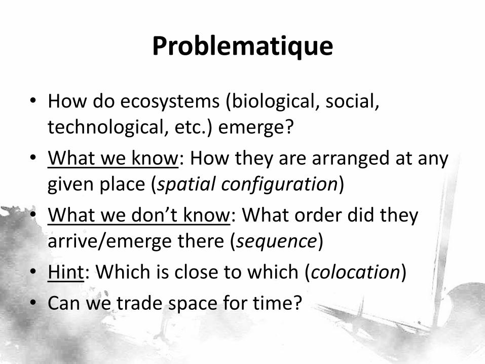
Problematique
• How do ecosystems (biological, social, technological, etc.) emerge?
• What we know: How they are arranged at any given place (spatial configuration)
• What we don’t know: What order did they arrive/emerge there (sequence)
• Hint: Which is close to which (colocation)
• Can we trade space for time?
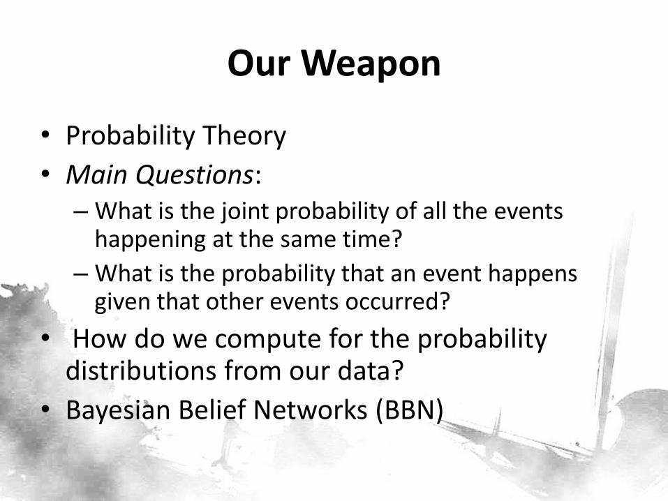
Our Weapon
• Probability Theory
• Main Questions: – What is the joint probability of all the events
happening at the same time?
– What is the probability that an event happens given that other events occurred?
• How do we compute for the probability distributions from our data?
• Bayesian Belief Networks (BBN)
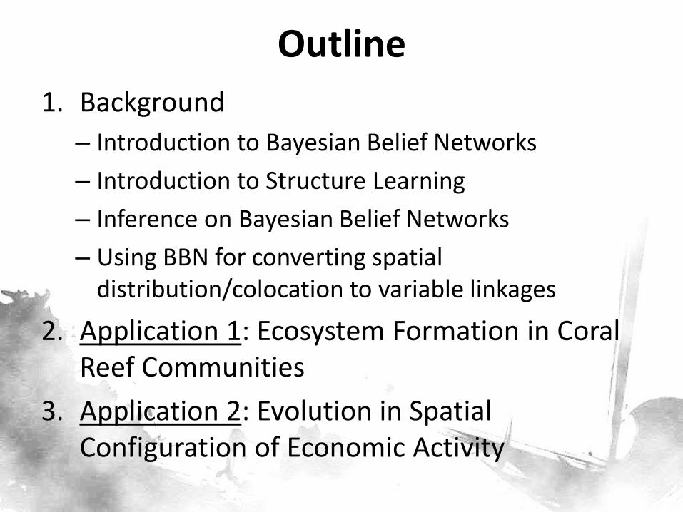
Outline
1. Background
– Introduction to Bayesian Belief Networks
– Introduction to Structure Learning
– Inference on Bayesian Belief Networks
– Using BBN for converting spatial distribution/colocation to variable linkages
2. Application 1: Ecosystem Formation in Coral Reef Communities
3. Application 2: Evolution in Spatial Configuration of Economic Activity
BAYESIAN BELIEF NETWORKS 1. Introduction to Bayesian Belief Networks
Bayesian Networks
• Bayesian networks (also called Bayes nets or Bayesian belief networks) are a way to depict the independence assumptions made in a distribution [Barber, 2012:31-32]
• Application domain widespread, ranging from troubleshooting and expert reasoning under uncertainty to machine learning.
• Uses structured conditional probability distributions (CPD) in modeling the problem.
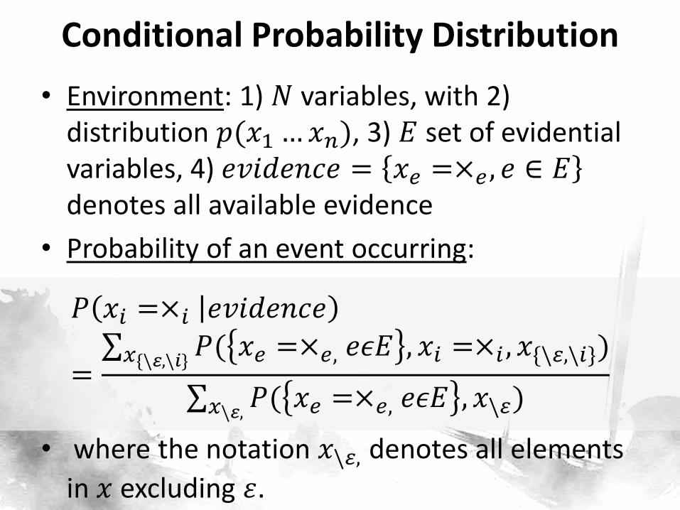
Conditional Probability Distribution
• Environment: 1) 𝑁 variables, with 2) distribution 𝑝(𝑥1…𝑥𝑛), 3) 𝐸 set of evidential variables, 4) 𝑒𝑣𝑖𝑑𝑒𝑛𝑐𝑒 = 𝑥𝑒 =×𝑒 , 𝑒 ∈ 𝐸 denotes all available evidence
• Probability of an event occurring:
𝑃 𝑥𝑖 =×𝑖 𝑒𝑣𝑖𝑑𝑒𝑛𝑐𝑒
= 𝑃( 𝑥𝑒 =×𝑒, 𝑒𝜖𝐸 , 𝑥𝑖 =×𝑖 , 𝑥{\𝜀,\𝑖})𝑥{\𝜀,\𝑖}
𝑃( 𝑥𝑒 =×𝑒, 𝑒𝜖𝐸 , 𝑥\𝜀)𝑥\𝜀,
• where the notation 𝑥\𝜀, denotes all elements
in 𝑥 excluding 𝜀.
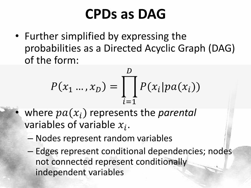
CPDs as DAG
• Further simplified by expressing the probabilities as a Directed Acyclic Graph (DAG) of the form:
𝑃 𝑥1… , 𝑥𝐷 = 𝑃(𝑥𝑖|𝑝𝑎(𝑥𝑖))
𝐷
𝑖=1
• where 𝑝𝑎(𝑥𝑖) represents the parental variables of variable 𝑥𝑖. – Nodes represent random variables
– Edges represent conditional dependencies; nodes not connected represent conditionally independent variables
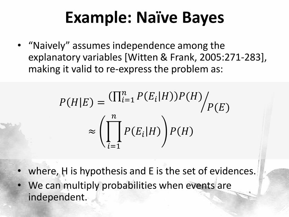
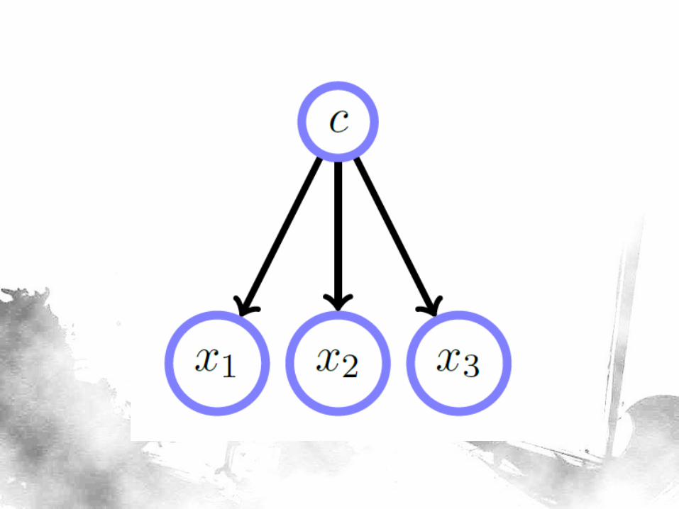
Example: Naïve Bayes
• “Naively” assumes independence among the explanatory variables [Witten & Frank, 2005:271-283], making it valid to re-express the problem as:
𝑃 𝐻 𝐸 = 𝑃 𝐸𝑖 𝐻𝑛𝑖=1 𝑃(𝐻)
𝑃(𝐸)
≈ 𝑃 𝐸𝑖 𝐻
𝑛
𝑖=1
𝑃 𝐻
• where, H is hypothesis and E is the set of evidences.
• We can multiply probabilities when events are independent.
Independence in Bayesian Networks
• How do Bayesian networks work?
• Helps us learn how information flows from variable to variable when we condition them (assign a certain value)
• Consequence of the CPDs – the joint distribution of the nodes can be expressed as a factor of the dependencies.
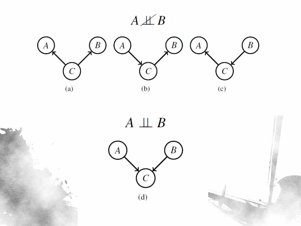
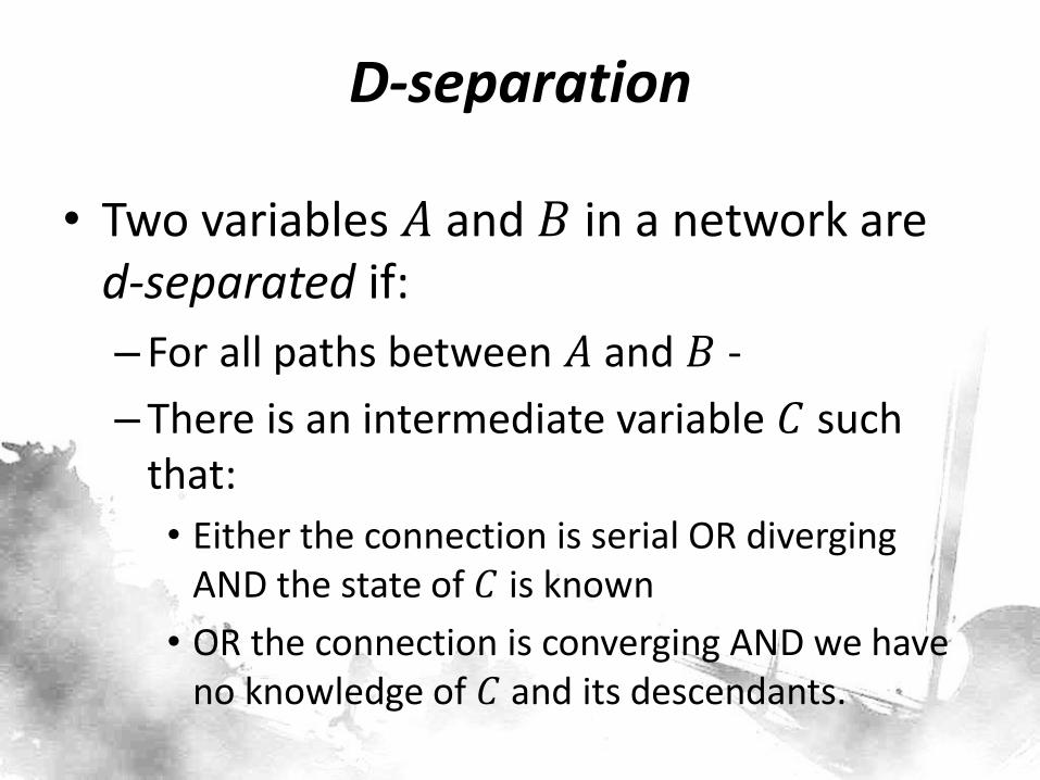
D-separation
• Two variables 𝐴 and 𝐵 in a network are d-separated if:
– For all paths between 𝐴 and 𝐵 -
– There is an intermediate variable 𝐶 such that:
• Either the connection is serial OR diverging AND the state of 𝐶 is known
• OR the connection is converging AND we have no knowledge of 𝐶 and its descendants.
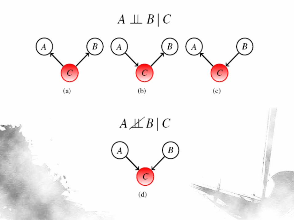
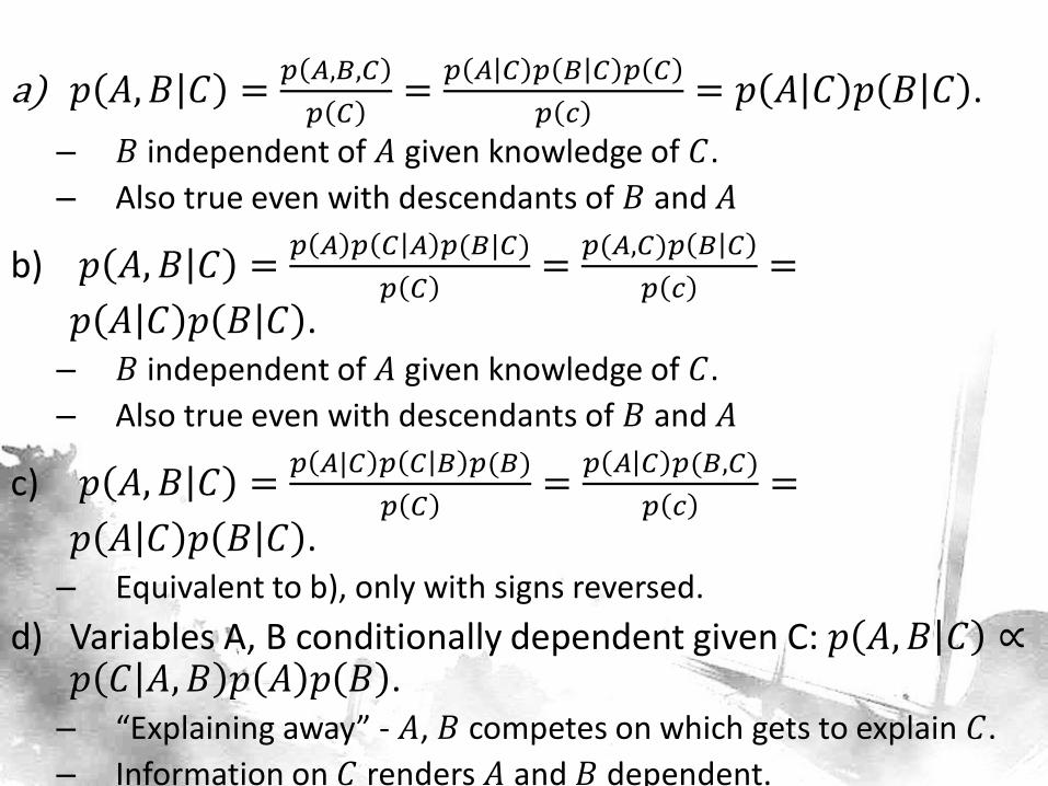
a) 𝑝 𝐴,𝐵 𝐶 =𝑝 𝐴,𝐵,𝐶
𝑝 𝐶=𝑝 𝐴 𝐶 𝑝 𝐵 𝐶 𝑝 𝐶
𝑝 𝑐= 𝑝 𝐴 𝐶 𝑝 𝐵 𝐶 .
– 𝐵 independent of 𝐴 given knowledge of 𝐶.
– Also true even with descendants of 𝐵 and 𝐴
b) 𝑝 𝐴, 𝐵 𝐶 =𝑝 𝐴 𝑝 𝐶 𝐴 𝑝(𝐵|𝐶)
𝑝 𝐶=𝑝(𝐴,𝐶)𝑝 𝐵 𝐶
𝑝 𝑐=
𝑝 𝐴 𝐶 𝑝 𝐵 𝐶 . – 𝐵 independent of 𝐴 given knowledge of 𝐶.
– Also true even with descendants of 𝐵 and 𝐴
c) 𝑝 𝐴, 𝐵 𝐶 =𝑝 𝐴|𝐶 𝑝 𝐶 𝐵 𝑝(𝐵)
𝑝 𝐶=𝑝 𝐴 𝐶 𝑝(𝐵,𝐶)
𝑝 𝑐=
𝑝 𝐴 𝐶 𝑝 𝐵 𝐶 . – Equivalent to b), only with signs reversed.
d) Variables A, B conditionally dependent given C: 𝑝 𝐴,𝐵 𝐶 ∝𝑝 𝐶 𝐴,𝐵 𝑝 𝐴 𝑝 𝐵 . – “Explaining away” - 𝐴, 𝐵 competes on which gets to explain 𝐶.
– Information on 𝐶 renders 𝐴 and 𝐵 dependent.
Tuberculosis
PresentAbsent
1.0499.0
XRay Result
AbnormalNormal
11.089.0
Tuberculosis or Cancer
TrueFalse
6.4893.5
Lung Cancer
PresentAbsent
5.5094.5
Dyspnea
PresentAbsent
43.656.4
Bronchitis
PresentAbsent
45.055.0
Visit To Asia
VisitNo Visi t
1.0099.0
Smoking
SmokerNonSmoker
50.050.0
Tuberculosis
PresentAbsent
5.0095.0
XRay Result
AbnormalNormal
14.585.5
Tuberculosis or Cancer
TrueFalse
10.289.8
Lung Cancer
PresentAbsent
5.5094.5
Dyspnea
PresentAbsent
45.055.0
Bronchitis
PresentAbsent
45.055.0
Visit To Asia
VisitNo Visi t
100 0
Smoking
SmokerNonSmoker
50.050.0
Tuberculosis
PresentAbsent
5.0095.0
XRay Result
AbnormalNormal
18.581.5
Tuberculosis or Cancer
TrueFalse
14.585.5
Lung Cancer
PresentAbsent
10.090.0
Dyspnea
PresentAbsent
56.443.6
Bronchitis
PresentAbsent
60.040.0
Visit To Asia
VisitNo Visi t
100 0
Smoking
SmokerNonSmoker
100 0
Tuberculosis
PresentAbsent
0.1299.9
XRay Result
AbnormalNormal
0 100
Tuberculosis or Cancer
TrueFalse
0.3699.6
Lung Cancer
PresentAbsent
0.2599.8
Dyspnea
PresentAbsent
52.147.9
Bronchitis
PresentAbsent
60.040.0
Visit To Asia
VisitNo Visi t
100 0
Smoking
SmokerNonSmoker
100 0
Tuberculosis
PresentAbsent
0.1999.8
XRay Result
AbnormalNormal
0 100
Tuberculosis or Cancer
TrueFalse
0.5699.4
Lung Cancer
PresentAbsent
0.3999.6
Dyspnea
PresentAbsent
100 0
Bronchitis
PresentAbsent
92.27.84
Visit To Asia
VisitNo Visi t
100 0
Smoking
SmokerNonSmoker
100 0
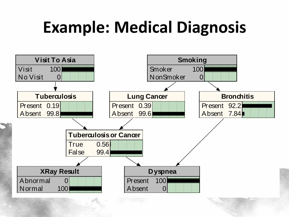
Example: Medical Diagnosis
Remarks: BBN as Classifier
• Bayesian Belief Networks are used as classifiers.
– How sets of variables explain classifier variable
• Present as data the set of states of the root and internal variables
• Deduce the most probable state of the leaf (or the root) node = classifier variable
• Important to note since algorithms that create BBN assume one classifier variable among the sets of variables
STRUCTURE LEARNING 1. Introduction to Bayesian Belief Networks
Building Bayesian Networks
• First, learn the network structure – the CPDs represented by a DAG.
• Second, compute the probability tables from the data.
– Straightforward
– Once structural conditional probabilistic dependencies are defined, empirically computing for the CPDs is next
Tree Augmented Network (TAN)
• For construction, we use the Tree Augmented Network (TAN) procedure.
• We begin with a Naïve Bayes, with a classifier node selected among the variables, and the rest are specified as evidence nodes.
• Evidence nodes are then connected into a tree through a Minimal Spanning Tree (MST) algo, using Mutual Information (MI) as weight.
• TAN is relatively simple to interpret.
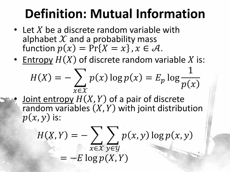
Definition: Mutual Information • Let 𝑋 be a discrete random variable with
alphabet 𝒳 and a probability mass function 𝑝 𝑥 = Pr 𝑋 = 𝑥 , 𝑥 ∈ 𝒜.
• Entropy 𝐻 𝑋 of discrete random variable 𝑋 is:
𝐻 𝑋 = − 𝑝 𝑥 log 𝑝 𝑥
𝑥∈𝒳
= 𝐸𝑝 log1
𝑝 𝑥
• Joint entropy 𝐻 𝑋, 𝑌 of a pair of discrete random variables 𝑋, 𝑌 with joint distribution 𝑝 𝑥, 𝑦 is:
𝐻 𝑋, 𝑌 = − 𝑝 𝑥, 𝑦 log 𝑝 𝑥, 𝑦
𝑦∈𝒴𝑥∈𝒳
= −𝐸 log 𝑝(𝑋, 𝑌)
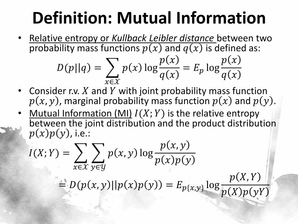
Definition: Mutual Information • Relative entropy or Kullback Leibler distance between two
probability mass functions 𝑝 𝑥 and 𝑞 𝑥 is defined as:
𝐷(𝑝| 𝑞 = 𝑝 𝑥 log𝑝 𝑥
𝑞 𝑥𝑥∈𝒳
= 𝐸𝑝 log𝑝 𝑥
𝑞 𝑥
• Consider r.v. 𝑋 and 𝑌 with joint probability mass function 𝑝 𝑥, 𝑦 , marginal probability mass function 𝑝 𝑥 and 𝑝 𝑦 .
• Mutual Information (MI) 𝐼(𝑋; 𝑌) is the relative entropy between the joint distribution and the product distribution 𝑝 𝑥 𝑝 𝑦 , i.e.:
𝐼(𝑋; 𝑌) = 𝑝 𝑥, 𝑦 log𝑝 𝑥, 𝑦
𝑝 𝑥 𝑝 𝑦𝑦∈𝒴𝑥∈𝒳
= 𝐷(𝑝 𝑥, 𝑦 | 𝑝 𝑥 𝑝 𝑦 = 𝐸𝑝{𝑥,𝑦} log𝑝 𝑋, 𝑌
𝑝 𝑋 𝑝 𝑦𝑌
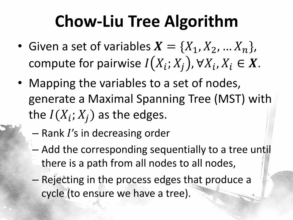
Chow-Liu Tree Algorithm
• Given a set of variables 𝑿 = {𝑋1, 𝑋2, … 𝑋𝑛},
compute for pairwise 𝐼 𝑋𝑖; 𝑋𝑗 , ∀𝑋𝑖 , 𝑋𝑖 ∈ 𝑿.
• Mapping the variables to a set of nodes, generate a Maximal Spanning Tree (MST) with the 𝐼(𝑋𝑖; 𝑋𝑗) as the edges.
– Rank 𝐼’s in decreasing order
– Add the corresponding sequentially to a tree until there is a path from all nodes to all nodes,
– Rejecting in the process edges that produce a cycle (to ensure we have a tree).
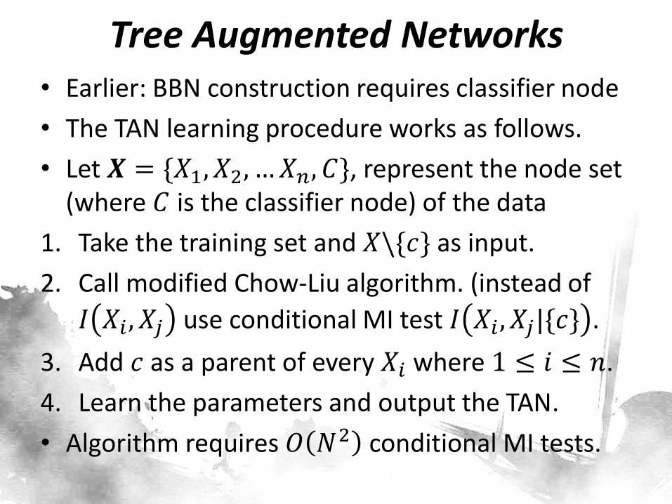
Tree Augmented Networks • Earlier: BBN construction requires classifier node
• The TAN learning procedure works as follows.
• Let 𝑿 = {𝑋1, 𝑋2, …𝑋𝑛, 𝐶}, represent the node set (where 𝐶 is the classifier node) of the data
1. Take the training set and 𝑋\{𝑐} as input.
2. Call modified Chow-Liu algorithm. (instead of
𝐼 𝑋𝑖 , 𝑋𝑗 use conditional MI test 𝐼 𝑋𝑖 , 𝑋𝑗|{𝑐} .
3. Add 𝑐 as a parent of every 𝑋𝑖 where 1 ≤ 𝑖 ≤ 𝑛.
4. Learn the parameters and output the TAN.
• Algorithm requires 𝑂 𝑁2 conditional MI tests.
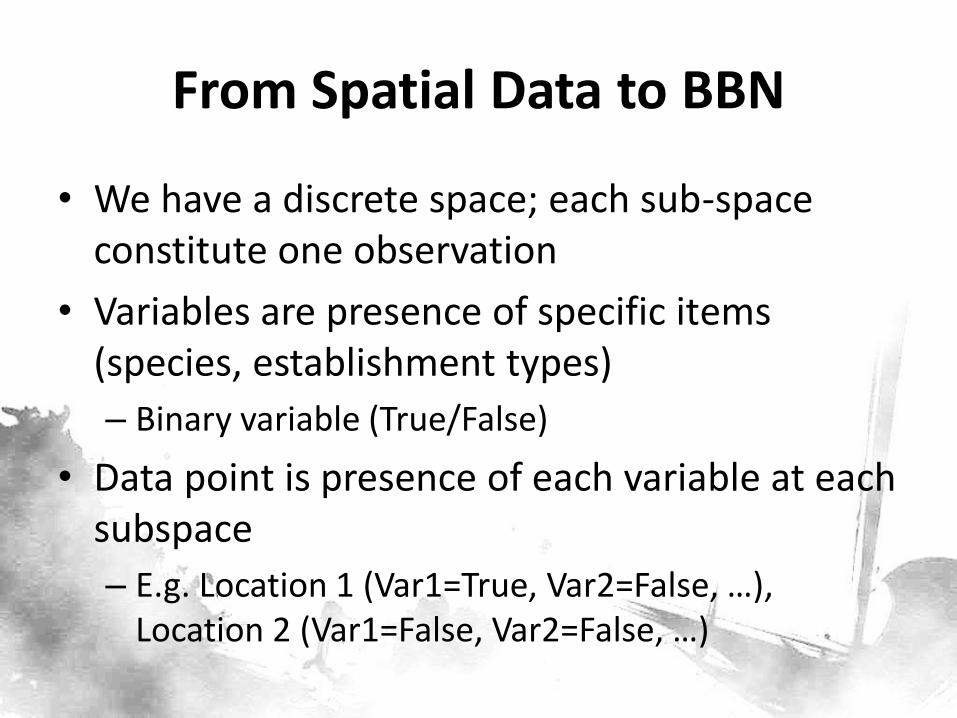
From Spatial Data to BBN
• We have a discrete space; each sub-space constitute one observation
• Variables are presence of specific items (species, establishment types)
– Binary variable (True/False)
• Data point is presence of each variable at each subspace
– E.g. Location 1 (Var1=True, Var2=False, …), Location 2 (Var1=False, Var2=False, …)

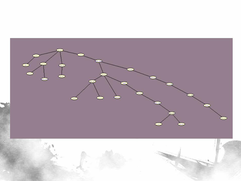
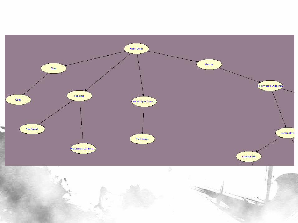
ECOSYSTEM FORMATION IN CORAL REEF COMMUNITIES
Application

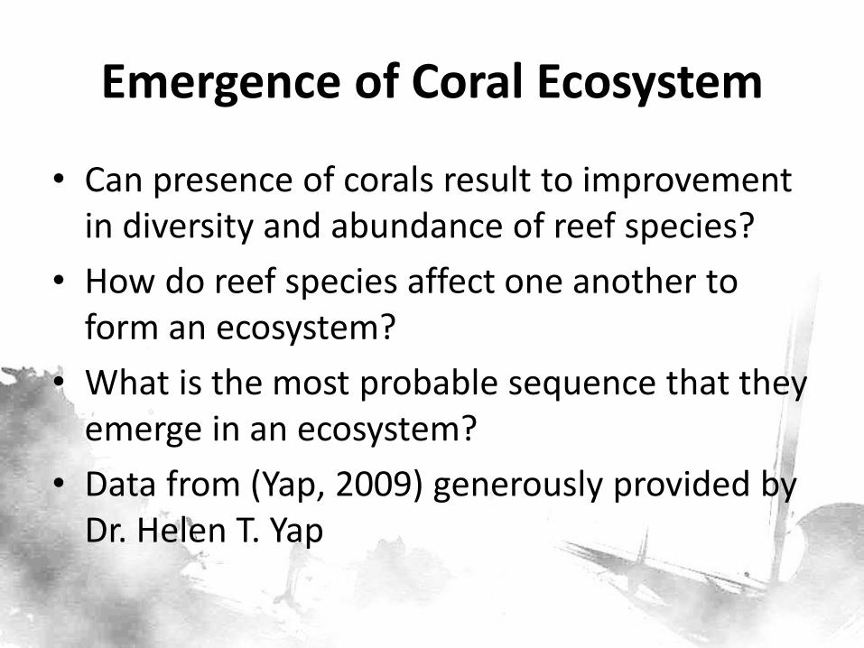
Emergence of Coral Ecosystem
• Can presence of corals result to improvement in diversity and abundance of reef species?
• How do reef species affect one another to form an ecosystem?
• What is the most probable sequence that they emerge in an ecosystem?
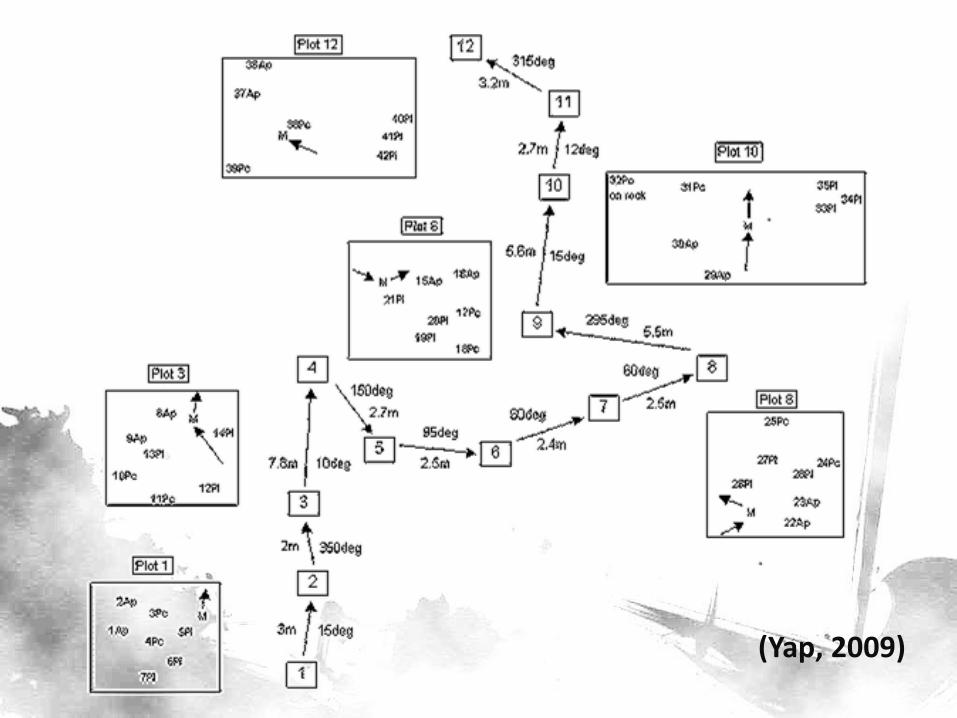
• Data from (Yap, 2009) generously provided by Dr. Helen T. Yap
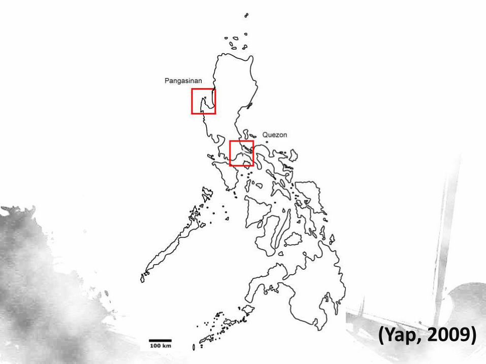
(Yap, 2009)
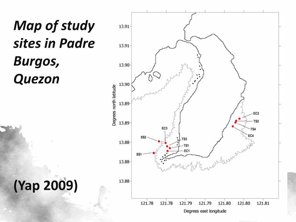
Map of study sites in Padre Burgos, Quezon
(Yap 2009)
(Yap, 2009)

(Yap, 2009)

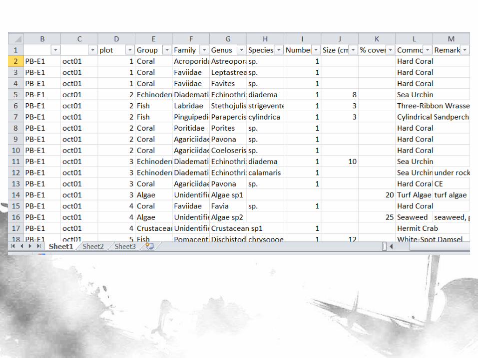

Data
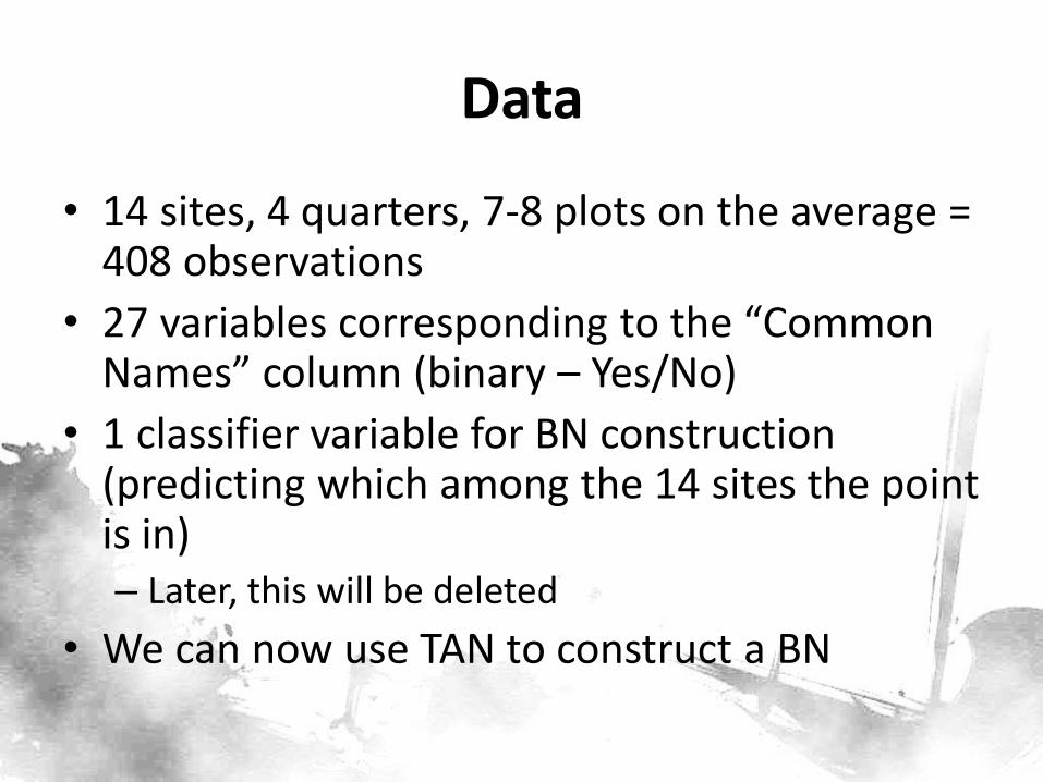
• 14 sites, 4 quarters, 7-8 plots on the average = 408 observations
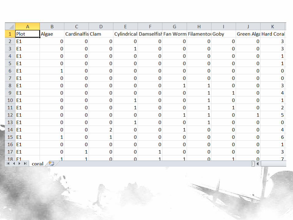
• 27 variables corresponding to the “Common Names” column (binary – Yes/No)
• 1 classifier variable for BN construction (predicting which among the 14 sites the point is in) – Later, this will be deleted
• We can now use TAN to construct a BN
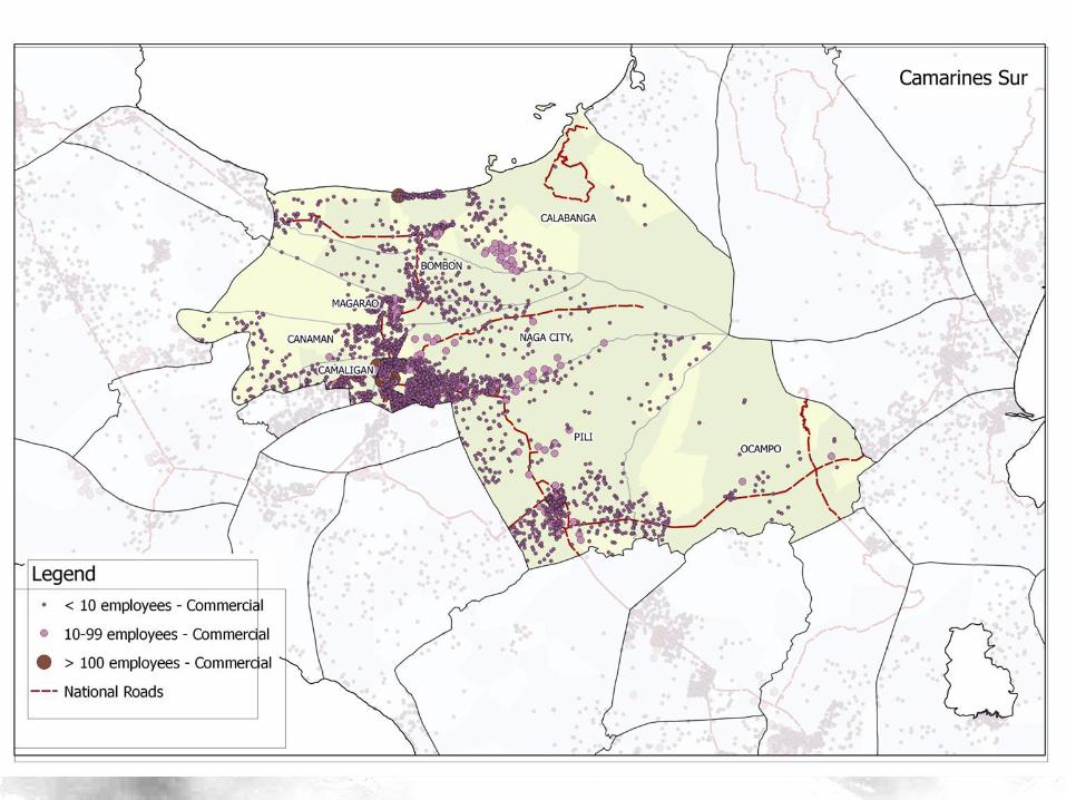
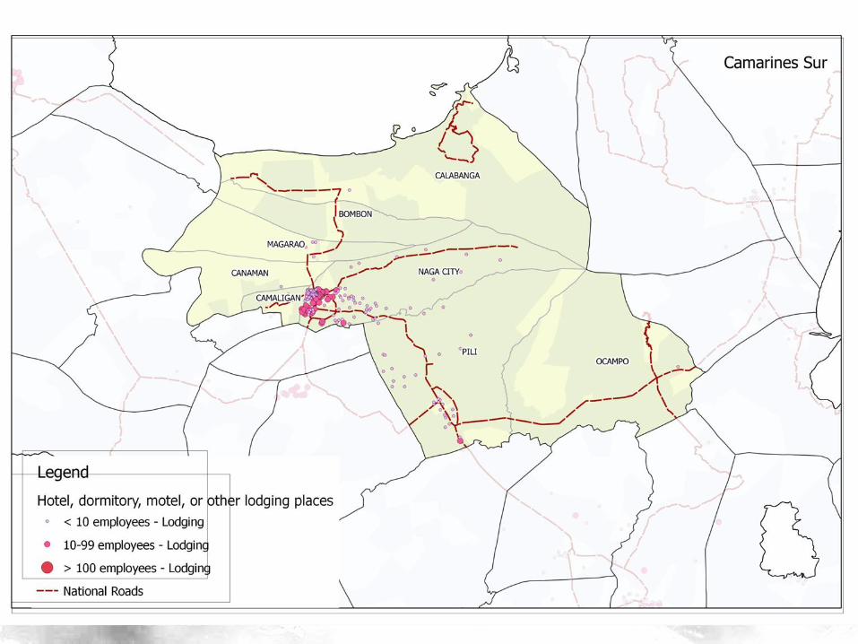
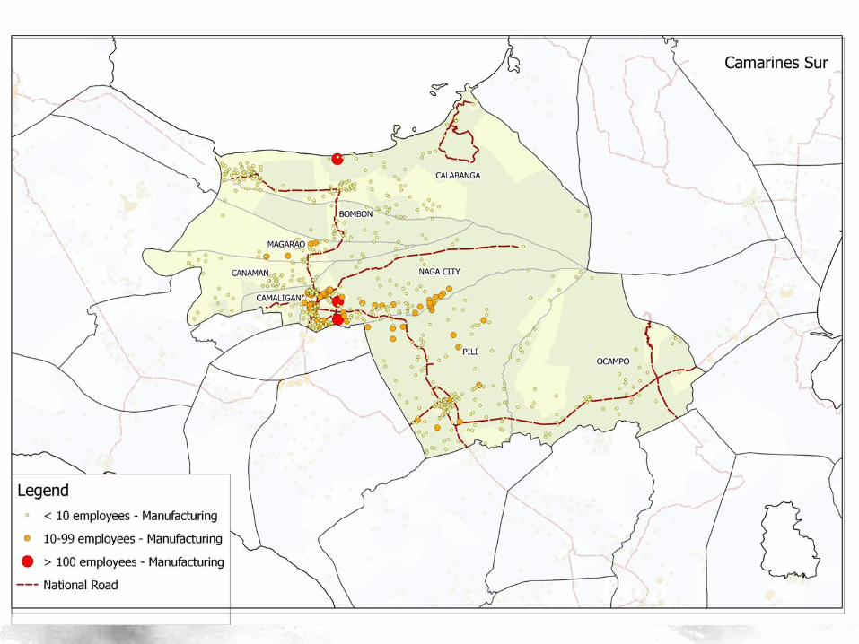
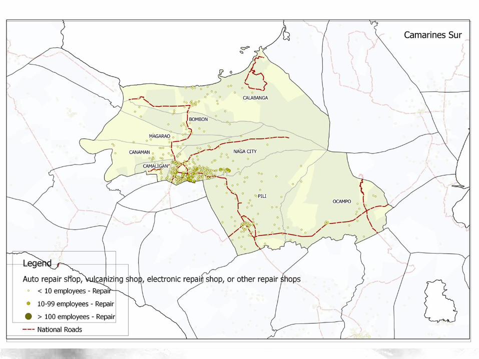
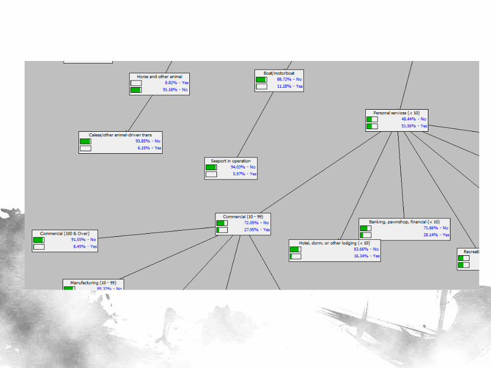
EVOLUTION IN SPATIAL CONFIGURATION OF ECONOMIC ACTIVITY
Application
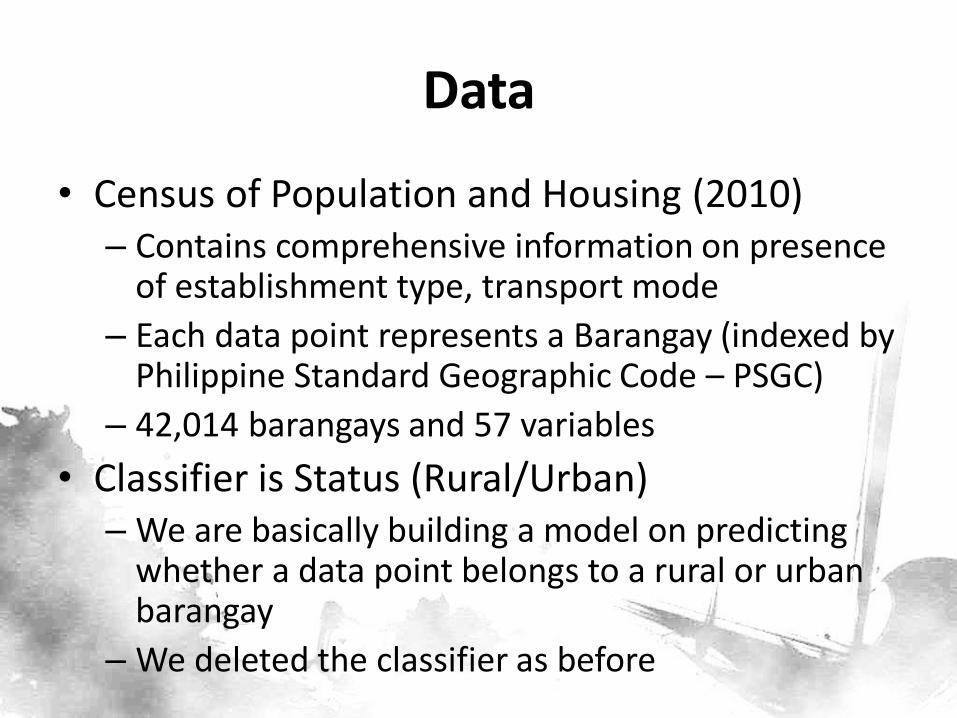
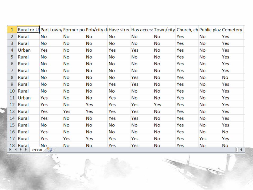
Data
• Census of Population and Housing (2010) – Contains comprehensive information on presence
of establishment type, transport mode
– Each data point represents a Barangay (indexed by Philippine Standard Geographic Code – PSGC)
– 42,014 barangays and 57 variables
• Classifier is Status (Rural/Urban) – We are basically building a model on predicting
whether a data point belongs to a rural or urban barangay
– We deleted the classifier as before
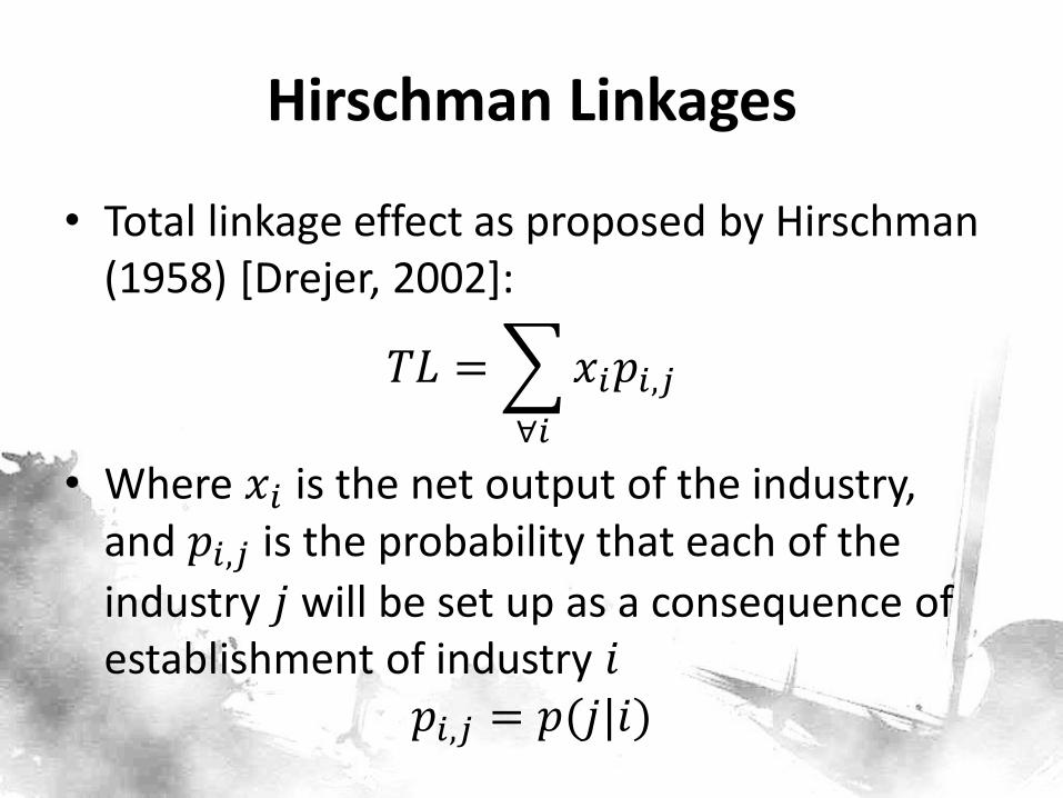
Hirschman Linkages
• Total linkage effect as proposed by Hirschman (1958) [Drejer, 2002]:
𝑇𝐿 = 𝑥𝑖𝑝𝑖,𝑗∀𝑖
• Where 𝑥𝑖 is the net output of the industry, and 𝑝𝑖,𝑗 is the probability that each of the
industry 𝑗 will be set up as a consequence of establishment of industry 𝑖
𝑝𝑖,𝑗 = 𝑝(𝑗|𝑖)
References
• Drejer, Ina (2002). Input-Output Based Measures of Interindustry Linkages Revisited – A Survey and Discussion. Centre for Economic and Business Research, Ministry of Economic and Business Affairs. Copenhagen, Denmark.
• Yap, Helen T. (2009). Local changes in community diversity after coral transplantation. Marine Ecology Progress Series. Vol. 374: 33–41, 2009.
General References
• Barber, D. (2012), Bayesian Reasoning and Machine Learning, pp. 31-32, 63-80.
• Cover, Thomas M. & Joy A. Thomas (1991). Elements of Information Theory, pp. 12-49.
• Cheng, Jie & Russel Greiner (1999). Comparing Bayesian Network Classifiers. Proceedings of the Fifteenth Conference Annual Conference on Uncertainty in Artificial Intelligence (UAI-99), pp. 101-108
• Witten, Ian H. & Eibe Frank (2005). Data Mining, pp. 271-283