Structure-generating mechanisms in agent-based...
64
Structure-generating mechanisms in agent-based models Rui Vilela Mendes (Institute) 1 / 25
Transcript of Structure-generating mechanisms in agent-based...

Structure-generating mechanisms in agent-based models
Rui Vilela Mendes
(Institute) 1 / 25

Organization, structure and patterns
Organization and structure are ubiquitous in natural phenomena
Pattern detected !�� obtain a compressed description� predict the outcome
�[Prediction through compressed descriptions is apparently the waymany living beings deal with the external world, ants includedReznikova and Ryabko; Problems Inf. Transmission 22 (1986) 245]Role of patterns and structures� Information processing tool for the observer� Determining factor in the coevolutionary process of compositesystemsUnderstanding patterns (or structures)Time series predictionStochastic model identi�cationDynamical system reconstructionCodingMeasures of complexity for patternsComputational mechanics
(Institute) 2 / 25
Organization, structure and patterns
Organization and structure are ubiquitous in natural phenomena
Pattern detected !�� obtain a compressed description� predict the outcome
�[Prediction through compressed descriptions is apparently the waymany living beings deal with the external world, ants includedReznikova and Ryabko; Problems Inf. Transmission 22 (1986) 245]
Role of patterns and structures� Information processing tool for the observer� Determining factor in the coevolutionary process of compositesystemsUnderstanding patterns (or structures)Time series predictionStochastic model identi�cationDynamical system reconstructionCodingMeasures of complexity for patternsComputational mechanics
(Institute) 2 / 25


Organization, structure and patterns
Organization and structure are ubiquitous in natural phenomena
Pattern detected !�� obtain a compressed description� predict the outcome
�[Prediction through compressed descriptions is apparently the waymany living beings deal with the external world, ants includedReznikova and Ryabko; Problems Inf. Transmission 22 (1986) 245]Role of patterns and structures� Information processing tool for the observer� Determining factor in the coevolutionary process of compositesystems
Understanding patterns (or structures)Time series predictionStochastic model identi�cationDynamical system reconstructionCodingMeasures of complexity for patternsComputational mechanics
(Institute) 2 / 25

Organization, structure and patterns
Organization and structure are ubiquitous in natural phenomena
Pattern detected !�� obtain a compressed description� predict the outcome
�[Prediction through compressed descriptions is apparently the waymany living beings deal with the external world, ants includedReznikova and Ryabko; Problems Inf. Transmission 22 (1986) 245]Role of patterns and structures� Information processing tool for the observer� Determining factor in the coevolutionary process of compositesystemsUnderstanding patterns (or structures)Time series predictionStochastic model identi�cationDynamical system reconstructionCoding
Measures of complexity for patternsComputational mechanics
(Institute) 2 / 25

Organization, structure and patterns
Organization and structure are ubiquitous in natural phenomena
Pattern detected !�� obtain a compressed description� predict the outcome
�[Prediction through compressed descriptions is apparently the waymany living beings deal with the external world, ants includedReznikova and Ryabko; Problems Inf. Transmission 22 (1986) 245]Role of patterns and structures� Information processing tool for the observer� Determining factor in the coevolutionary process of compositesystemsUnderstanding patterns (or structures)Time series predictionStochastic model identi�cationDynamical system reconstructionCodingMeasures of complexity for patterns
Computational mechanics
(Institute) 2 / 25

Organization, structure and patterns
Organization and structure are ubiquitous in natural phenomena
Pattern detected !�� obtain a compressed description� predict the outcome
�[Prediction through compressed descriptions is apparently the waymany living beings deal with the external world, ants includedReznikova and Ryabko; Problems Inf. Transmission 22 (1986) 245]Role of patterns and structures� Information processing tool for the observer� Determining factor in the coevolutionary process of compositesystemsUnderstanding patterns (or structures)Time series predictionStochastic model identi�cationDynamical system reconstructionCodingMeasures of complexity for patternsComputational mechanics
(Institute) 2 / 25

Dynamical mechanisms leading to collective structures
Why is the dynamical behavior of a composite system qualitativelydi¤erent from the dynamics of the components in isolation?
Collective structure formation in systems composed of many agents ininteraction, each one of which has simple dynamics.(simple to describe in law, but not necessarily with simple orbits.Small logic depth, but capable of generating orbits with highKolmogorov complexity) Example:
xn+1 = pxn (mod .1)
- Invariant measure absolutely continuous with respect to Lebesgue,- Positive Lyapunov exponents and Kolmogorov entropy,- Orbits of all typesMechanisms(1) Sensitive-dependence and convex coupling(2) Sensitive-dependence and extremal dynamics(3) Interaction through a collectively generated �eld. (Multistabilityand evolution)
(Institute) 3 / 25

Dynamical mechanisms leading to collective structures
Why is the dynamical behavior of a composite system qualitativelydi¤erent from the dynamics of the components in isolation?Collective structure formation in systems composed of many agents ininteraction, each one of which has simple dynamics.(simple to describe in law, but not necessarily with simple orbits.Small logic depth, but capable of generating orbits with highKolmogorov complexity) Example:
xn+1 = pxn (mod .1)
- Invariant measure absolutely continuous with respect to Lebesgue,- Positive Lyapunov exponents and Kolmogorov entropy,- Orbits of all types
Mechanisms(1) Sensitive-dependence and convex coupling(2) Sensitive-dependence and extremal dynamics(3) Interaction through a collectively generated �eld. (Multistabilityand evolution)
(Institute) 3 / 25

Dynamical mechanisms leading to collective structures
Why is the dynamical behavior of a composite system qualitativelydi¤erent from the dynamics of the components in isolation?Collective structure formation in systems composed of many agents ininteraction, each one of which has simple dynamics.(simple to describe in law, but not necessarily with simple orbits.Small logic depth, but capable of generating orbits with highKolmogorov complexity) Example:
xn+1 = pxn (mod .1)
- Invariant measure absolutely continuous with respect to Lebesgue,- Positive Lyapunov exponents and Kolmogorov entropy,- Orbits of all typesMechanisms(1) Sensitive-dependence and convex coupling(2) Sensitive-dependence and extremal dynamics(3) Interaction through a collectively generated �eld. (Multistabilityand evolution)
(Institute) 3 / 25

Structure-generation through density-dependent coupling
Bernoulli agents on circle with nearest-neighbour convex coupling
xi (t + 1) = (1� c)f (xi (t)) +c2(f (xi+1(t)) + f (xi�1(t))) (1)
f (x) = 2x (mod. 1) and periodic boundary conditions
Agents assumed to live in a limited space with the intensity of thecoupling a function of the total number of agents N, for example
c = cm�1� e�αN
�(2)
Coupling is also dynamical by a reproduction and death mechanism- After each R time cycles, agents with xi > 0.5 are coded 1 andthose with xi � 0.5 are coded 0.- Con�gurations 0110 :candidates for reproduction with probability pr- Con�gurations 0000 :candidates for death with probability pm- Reproduction : transition 0110 ! 0X110 , the state of the newagent X chosen at random in the interval (0, 1)- Death : transition 0000 ! 000
(Institute) 4 / 25

Structure-generation through density-dependent coupling
Bernoulli agents on circle with nearest-neighbour convex coupling
xi (t + 1) = (1� c)f (xi (t)) +c2(f (xi+1(t)) + f (xi�1(t))) (1)
f (x) = 2x (mod. 1) and periodic boundary conditionsAgents assumed to live in a limited space with the intensity of thecoupling a function of the total number of agents N, for example
c = cm�1� e�αN
�(2)
Coupling is also dynamical by a reproduction and death mechanism- After each R time cycles, agents with xi > 0.5 are coded 1 andthose with xi � 0.5 are coded 0.- Con�gurations 0110 :candidates for reproduction with probability pr- Con�gurations 0000 :candidates for death with probability pm- Reproduction : transition 0110 ! 0X110 , the state of the newagent X chosen at random in the interval (0, 1)- Death : transition 0000 ! 000
(Institute) 4 / 25

Structure-generation through density-dependent coupling
Without coupling 0110 and 0000 appear, on average, the samenumber of times. The population density depends only on the relativevalues of pr and pm .
With coupling: correlations, generated by coupling, in�uence theinter-agent evolution mechanismThe Lyapunov exponents for the dynamical system in (1) are
λk = log�2 (1� c) + 2c cos
�2π
nk��
k = 0, � � � ,N � 1
All positive for c < 0.5 but above this value structures are createdwhen each Lyapunov exponent crosses zero. Collective modes havedi¤erent probabilities, a new collective mode being frozen each time aLyapunov exponent reaches the zero value.The eigenvectors corresponding to each exponent are
�e inθk
with
θk =2πN k , k = 0, � � � ,N � 1. Therefore yk =
1N ∑N
n=1 cos� 2πN kn
�are the coordinates of the collective eigenmodes
(Institute) 5 / 25

Structure-generation through density-dependent coupling
Without coupling 0110 and 0000 appear, on average, the samenumber of times. The population density depends only on the relativevalues of pr and pm .With coupling: correlations, generated by coupling, in�uence theinter-agent evolution mechanism
The Lyapunov exponents for the dynamical system in (1) are
λk = log�2 (1� c) + 2c cos
�2π
nk��
k = 0, � � � ,N � 1
All positive for c < 0.5 but above this value structures are createdwhen each Lyapunov exponent crosses zero. Collective modes havedi¤erent probabilities, a new collective mode being frozen each time aLyapunov exponent reaches the zero value.The eigenvectors corresponding to each exponent are
�e inθk
with
θk =2πN k , k = 0, � � � ,N � 1. Therefore yk =
1N ∑N
n=1 cos� 2πN kn
�are the coordinates of the collective eigenmodes
(Institute) 5 / 25

Structure-generation through density-dependent coupling
Without coupling 0110 and 0000 appear, on average, the samenumber of times. The population density depends only on the relativevalues of pr and pm .With coupling: correlations, generated by coupling, in�uence theinter-agent evolution mechanismThe Lyapunov exponents for the dynamical system in (1) are
λk = log�2 (1� c) + 2c cos
�2π
nk��
k = 0, � � � ,N � 1
All positive for c < 0.5 but above this value structures are createdwhen each Lyapunov exponent crosses zero. Collective modes havedi¤erent probabilities, a new collective mode being frozen each time aLyapunov exponent reaches the zero value.
The eigenvectors corresponding to each exponent are�e inθk
with
θk =2πN k , k = 0, � � � ,N � 1. Therefore yk =
1N ∑N
n=1 cos� 2πN kn
�are the coordinates of the collective eigenmodes
(Institute) 5 / 25

Structure-generation through density-dependent coupling
Without coupling 0110 and 0000 appear, on average, the samenumber of times. The population density depends only on the relativevalues of pr and pm .With coupling: correlations, generated by coupling, in�uence theinter-agent evolution mechanismThe Lyapunov exponents for the dynamical system in (1) are
λk = log�2 (1� c) + 2c cos
�2π
nk��
k = 0, � � � ,N � 1
All positive for c < 0.5 but above this value structures are createdwhen each Lyapunov exponent crosses zero. Collective modes havedi¤erent probabilities, a new collective mode being frozen each time aLyapunov exponent reaches the zero value.The eigenvectors corresponding to each exponent are
�e inθk
with
θk =2πN k , k = 0, � � � ,N � 1. Therefore yk =
1N ∑N
n=1 cos� 2πN kn
�are the coordinates of the collective eigenmodes
(Institute) 5 / 25
Structure-generation through density-dependent coupling
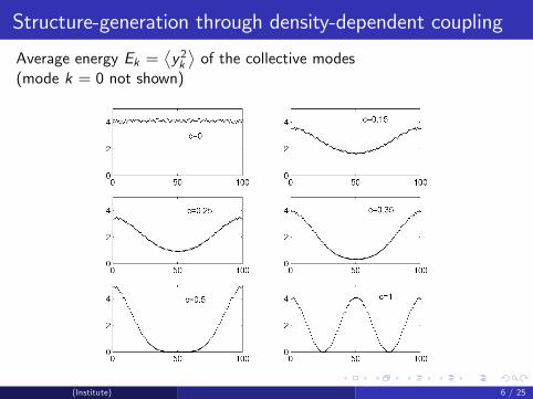
Average energy Ek =y2k�of the collective modes
(mode k = 0 not shown)
(Institute) 6 / 25

Structure-generation through density-dependent coupling
Evolution of the population plotted against the reproduction-death cyclenumber (pr = 1 and pm = 0.5). Population controlled by collectivestructures
(Institute) 7 / 25

Structure-generation through density-dependent coupling
Relative probability of each one of the 16 di¤erent con�gurations of fourneighbours (x1x2x3x4), labelled by x1 + 2� x2 + 4� x2 + 8� x2
(Institute) 8 / 25

Interaction through collective variables
Interaction mediated by a collective variable, that is an aggregatequantity that the agents themselves create
In most models there is also an evolution mechanism
Multistability and evolution :In some cases, the essential mechanism, self-organizing the system, isthe evolution (a slow dynamics), the fast dynamics only provides themulti-attractor background which is selected by the slow evolution.
(Institute) 9 / 25

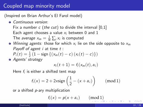
Coupled map minority model
(Inspired on Brian Arthur�s El Farol model)
Continuous version:Fix a number c (the cut) to divide the interval [0,1]Each agent chooses a value xi between 0 and 1The average xm = 1
N ∑i xi is computed
Winning agents: those for which xi lie on the side opposite to xmPayo¤ of agent i at time t :Pi (t) = 1
2 (1� sign f(xm(t)� c) (xi (t)� c)g)Agents�strategy
xi (t + 1) = fi (xm(t), αi )
Here fi is either a shifted tent map
fi (x) = 2+ 2xsign�12� (x + αi )
�(mod 1)
or a shifted p-ary multiplication
fi (x) = p(x + αi ) (mod 1)
(Institute) 10 / 25

Coupled map minority model
(Inspired on Brian Arthur�s El Farol model)
Continuous version:Fix a number c (the cut) to divide the interval [0,1]Each agent chooses a value xi between 0 and 1The average xm = 1
N ∑i xi is computedWinning agents: those for which xi lie on the side opposite to xmPayo¤ of agent i at time t :Pi (t) = 1
2 (1� sign f(xm(t)� c) (xi (t)� c)g)
Agents�strategyxi (t + 1) = fi (xm(t), αi )
Here fi is either a shifted tent map
fi (x) = 2+ 2xsign�12� (x + αi )
�(mod 1)
or a shifted p-ary multiplication
fi (x) = p(x + αi ) (mod 1)
(Institute) 10 / 25
Coupled map minority model
(Inspired on Brian Arthur�s El Farol model)
Continuous version:Fix a number c (the cut) to divide the interval [0,1]Each agent chooses a value xi between 0 and 1The average xm = 1
N ∑i xi is computedWinning agents: those for which xi lie on the side opposite to xmPayo¤ of agent i at time t :Pi (t) = 1
2 (1� sign f(xm(t)� c) (xi (t)� c)g)Agents�strategy
xi (t + 1) = fi (xm(t), αi )
Here fi is either a shifted tent map
fi (x) = 2+ 2xsign�12� (x + αi )
�(mod 1)
or a shifted p-ary multiplication
fi (x) = p(x + αi ) (mod 1)
(Institute) 10 / 25

Coupled map minority model
αi is a number between zero and one and at t = 0 the strategies (theαi�s) are random
Evolution: Each r time steps k agents have their strategies modi�ed# The k 0agents with less earnings in that period have new (random)α�s# The remaining k � k 0 copy the α�s of the k � k 0 best performerswith a small error
Behavior of the model : Approach to a regime where the averagevalue xm oscillates around the value of the cut c (even when c is verydi¤erent from the random value 0.5)
P =fraction of winning agents
P =1N ∑
iPi
(Institute) 11 / 25

Coupled map minority model
Shifted tent map(N = 100, k = r = 10 and k
0= 3)
(Institute) 12 / 25
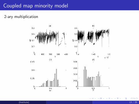
Coupled map minority model
2-ary multiplication
(Institute) 13 / 25
Coupled map minority model
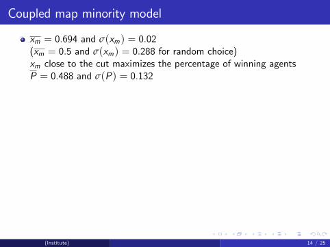
xm = 0.694 and σ(xm) = 0.02(xm = 0.5 and σ(xm) = 0.288 for random choice)xm close to the cut maximizes the percentage of winning agentsP = 0.488 and σ(P) = 0.132
The Lyapunov exponents for the dynamics of xm and for the dynamicsof the agents control the �uctuationsThe dynamics of xm is
xm(t + 1) =1N ∑
ifi (xm(t) + αi )
the Lyapunov exponent being
λ = limk!∞
1klog
1N
�����∑i f 0i (xm(t) + αi )
����� � � � 1N�����∑i f 0i (xm(t + k) + αi )
�����!
(Institute) 14 / 25
Coupled map minority model
xm = 0.694 and σ(xm) = 0.02(xm = 0.5 and σ(xm) = 0.288 for random choice)xm close to the cut maximizes the percentage of winning agentsP = 0.488 and σ(P) = 0.132The Lyapunov exponents for the dynamics of xm and for the dynamicsof the agents control the �uctuations
The dynamics of xm is
xm(t + 1) =1N ∑
ifi (xm(t) + αi )
the Lyapunov exponent being
λ = limk!∞
1klog
1N
�����∑i f 0i (xm(t) + αi )
����� � � � 1N�����∑i f 0i (xm(t + k) + αi )
�����!
(Institute) 14 / 25

Coupled map minority model
xm = 0.694 and σ(xm) = 0.02(xm = 0.5 and σ(xm) = 0.288 for random choice)xm close to the cut maximizes the percentage of winning agentsP = 0.488 and σ(P) = 0.132The Lyapunov exponents for the dynamics of xm and for the dynamicsof the agents control the �uctuationsThe dynamics of xm is
xm(t + 1) =1N ∑
ifi (xm(t) + αi )
the Lyapunov exponent being
λ = limk!∞
1klog
1N
�����∑i f 0i (xm(t) + αi )
����� � � � 1N�����∑i f 0i (xm(t + k) + αi )
�����!
(Institute) 14 / 25

Coupled map minority model
For the tent map: for a large number agents, uniform distribution ofthe α�s, 1N j∑i f
0i j of order 1p
N, =) λ negative of order � 1
2 logN
For the p-ary map λ = p.Dynamics of the agents: Jacobian matrix is
DT =
0BBBB@1N f
01
1N f
01 � � � 1
N f01
......
......
......
1N f
0N
1N f
0N � � � 1
N f0N
1CCCCAEigenvalues of
�DT k
�T �DT k
�are N � 1 zeros and one equal to
N
1N2 ∑
if 02i
! 1N ∑
if 0i
!2� � � 1N ∑
if 0i
!2One non-trivial Lyapunov exponent identical to the Lyapunovexponent of the xm dynamics.
(Institute) 15 / 25

Coupled map minority model
For the tent map: for a large number agents, uniform distribution ofthe α�s, 1N j∑i f
0i j of order 1p
N, =) λ negative of order � 1
2 logNFor the p-ary map λ = p.
Dynamics of the agents: Jacobian matrix is
DT =
0BBBB@1N f
01
1N f
01 � � � 1
N f01
......
......
......
1N f
0N
1N f
0N � � � 1
N f0N
1CCCCAEigenvalues of
�DT k
�T �DT k
�are N � 1 zeros and one equal to
N
1N2 ∑
if 02i
! 1N ∑
if 0i
!2� � � 1N ∑
if 0i
!2One non-trivial Lyapunov exponent identical to the Lyapunovexponent of the xm dynamics.
(Institute) 15 / 25

Coupled map minority model
For the tent map: for a large number agents, uniform distribution ofthe α�s, 1N j∑i f
0i j of order 1p
N, =) λ negative of order � 1
2 logNFor the p-ary map λ = p.Dynamics of the agents: Jacobian matrix is
DT =
0BBBB@1N f
01
1N f
01 � � � 1
N f01
......
......
......
1N f
0N
1N f
0N � � � 1
N f0N
1CCCCA
Eigenvalues of�DT k
�T �DT k
�are N � 1 zeros and one equal to
N
1N2 ∑
if 02i
! 1N ∑
if 0i
!2� � � 1N ∑
if 0i
!2One non-trivial Lyapunov exponent identical to the Lyapunovexponent of the xm dynamics.
(Institute) 15 / 25
Coupled map minority model
For the tent map: for a large number agents, uniform distribution ofthe α�s, 1N j∑i f
0i j of order 1p
N, =) λ negative of order � 1
2 logNFor the p-ary map λ = p.Dynamics of the agents: Jacobian matrix is
DT =
0BBBB@1N f
01
1N f
01 � � � 1
N f01
......
......
......
1N f
0N
1N f
0N � � � 1
N f0N
1CCCCAEigenvalues of
�DT k
�T �DT k
�are N � 1 zeros and one equal to
N
1N2 ∑
if 02i
! 1N ∑
if 0i
!2� � � 1N ∑
if 0i
!2One non-trivial Lyapunov exponent identical to the Lyapunovexponent of the xm dynamics.
(Institute) 15 / 25

Coupled map minority model
Features:1 - the evolution dynamics organizes the system (xm around the cut)2 - the fast dynamics controls the nature of the �uctuations aroundthis value3 - behavior of the collective variable around the average value isquite irregular. Compatible with the fast contraction of negativeLyapunov exponents because of sensitivity of the attractor to smallchanges of parameters
p�ary map:large �uctuations around the mean collective valuexm = 0.554, σ(xm) = 0.145, P = 0.378 and σ(P) = 0.223
Non-periodic attractors.
In conclusion: self-organization is driven by the slow (evolution)dynamics on the attractor background supplied by the (fast) agentdynamics
(Institute) 16 / 25
A market-like game
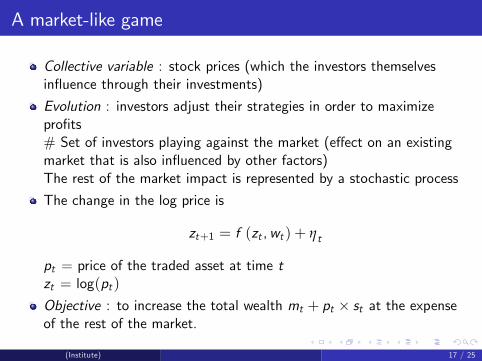
Collective variable : stock prices (which the investors themselvesin�uence through their investments)
Evolution : investors adjust their strategies in order to maximizepro�ts# Set of investors playing against the market (e¤ect on an existingmarket that is also in�uenced by other factors)The rest of the market impact is represented by a stochastic process
The change in the log price is
zt+1 = f (zt ,wt ) + ηt
pt = price of the traded asset at time tzt = log(pt )
Objective : to increase the total wealth mt + pt � st at the expenseof the rest of the market.
(Institute) 17 / 25

A market-like game
Collective variable : stock prices (which the investors themselvesin�uence through their investments)
Evolution : investors adjust their strategies in order to maximizepro�ts# Set of investors playing against the market (e¤ect on an existingmarket that is also in�uenced by other factors)The rest of the market impact is represented by a stochastic process
The change in the log price is
zt+1 = f (zt ,wt ) + ηt
pt = price of the traded asset at time tzt = log(pt )
Objective : to increase the total wealth mt + pt � st at the expenseof the rest of the market.
(Institute) 17 / 25

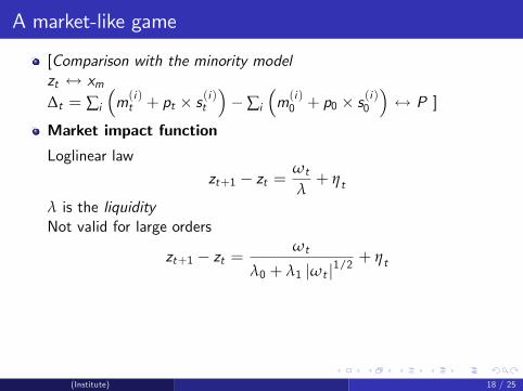
A market-like game
[Comparison with the minority modelzt $ xm∆t = ∑i
�m(i )t + pt � s(i )t
��∑i
�m(i )0 + p0 � s(i )0
�$ P ]
Market impact function
Loglinear law
zt+1 � zt =ωt
λ+ ηt
λ is the liquidityNot valid for large orders
zt+1 � zt =ωt
λ0 + λ1 jωt j1/2 + ηt
Agent strategies
Two types of informations are taken into account:The misprice
zvt � zt = log(vt )� log(pt )
(Institute) 18 / 25

A market-like game
[Comparison with the minority modelzt $ xm∆t = ∑i
�m(i )t + pt � s(i )t
��∑i
�m(i )0 + p0 � s(i )0
�$ P ]
Market impact function
Loglinear law
zt+1 � zt =ωt
λ+ ηt
λ is the liquidityNot valid for large orders
zt+1 � zt =ωt
λ0 + λ1 jωt j1/2 + ηt
Agent strategies
Two types of informations are taken into account:The misprice
zvt � zt = log(vt )� log(pt )(Institute) 18 / 25

A market-like game
and the price trend
zt � zt�1 = log(pt )� log(pt�1)
# Non-decreasing function f (x) such that f (�∞) = 0 and f (∞) = 1Two examples
f1(x) = θ(x)f2(x) = 1
1+exp(�βx )
Four-component vector γ
γt =
0BB@f (zvt � zt )f (zt � zt�1)
f (zvt � zt ) (1� f (zt � zt�1))(1� f (zvt � zt )) f (zt � zt�1)
(1� f (zvt � zt )) (1� f (zt � zt�1))
1CCAStrategy of each investor :four-component vector α(i ) with entries �1, 0, or 1Investment of agent i : α(i ) � γ
(Institute) 19 / 25

A market-like game
and the price trend
zt � zt�1 = log(pt )� log(pt�1)
# Non-decreasing function f (x) such that f (�∞) = 0 and f (∞) = 1Two examples
f1(x) = θ(x)f2(x) = 1
1+exp(�βx )
Four-component vector γ
γt =
0BB@f (zvt � zt )f (zt � zt�1)
f (zvt � zt ) (1� f (zt � zt�1))(1� f (zvt � zt )) f (zt � zt�1)
(1� f (zvt � zt )) (1� f (zt � zt�1))
1CCA
Strategy of each investor :four-component vector α(i ) with entries �1, 0, or 1Investment of agent i : α(i ) � γ
(Institute) 19 / 25

A market-like game
and the price trend
zt � zt�1 = log(pt )� log(pt�1)
# Non-decreasing function f (x) such that f (�∞) = 0 and f (∞) = 1Two examples
f1(x) = θ(x)f2(x) = 1
1+exp(�βx )
Four-component vector γ
γt =
0BB@f (zvt � zt )f (zt � zt�1)
f (zvt � zt ) (1� f (zt � zt�1))(1� f (zvt � zt )) f (zt � zt�1)
(1� f (zvt � zt )) (1� f (zt � zt�1))
1CCAStrategy of each investor :four-component vector α(i ) with entries �1, 0, or 1Investment of agent i : α(i ) � γ
(Institute) 19 / 25

A market-like game
Examples:Fundamental (value-investing strategy)α(i ) = (1, 1,�1,�1)Pure trend-following (technical trading)α(i ) = (1,�1, 1,�1)
Total number of strategies is 34 = 81. Strategies labelled by a number
n(i ) =3
∑k=0
3k�
α(i )k + 1
�(Fundamental strategy = no.72 and pure trend-following = no.60)Evolution dynamics :- After r time steps s agents copy the strategy of the s bestperformers plus- Mutation probability(In the �gures: r = 50, s = 10, λ0 = 10000), 45 = (0, 1,�1,�1),18 = (�1, 1,�1,�1), 73 = (1, 1,�1, 0), 75 = (1, 1, 0,�1)
(Institute) 20 / 25

A market-like game
Examples:Fundamental (value-investing strategy)α(i ) = (1, 1,�1,�1)Pure trend-following (technical trading)α(i ) = (1,�1, 1,�1)Total number of strategies is 34 = 81. Strategies labelled by a number
n(i ) =3
∑k=0
3k�
α(i )k + 1
�(Fundamental strategy = no.72 and pure trend-following = no.60)
Evolution dynamics :- After r time steps s agents copy the strategy of the s bestperformers plus- Mutation probability(In the �gures: r = 50, s = 10, λ0 = 10000), 45 = (0, 1,�1,�1),18 = (�1, 1,�1,�1), 73 = (1, 1,�1, 0), 75 = (1, 1, 0,�1)
(Institute) 20 / 25

A market-like game
Examples:Fundamental (value-investing strategy)α(i ) = (1, 1,�1,�1)Pure trend-following (technical trading)α(i ) = (1,�1, 1,�1)Total number of strategies is 34 = 81. Strategies labelled by a number
n(i ) =3
∑k=0
3k�
α(i )k + 1
�(Fundamental strategy = no.72 and pure trend-following = no.60)Evolution dynamics :- After r time steps s agents copy the strategy of the s bestperformers plus- Mutation probability(In the �gures: r = 50, s = 10, λ0 = 10000), 45 = (0, 1,�1,�1),18 = (�1, 1,�1,�1), 73 = (1, 1,�1, 0), 75 = (1, 1, 0,�1)
(Institute) 20 / 25

A market-like game
Market game simulation with evolution. Initial condition: all traders in thefundamental strategy
4 2 0 2 410 5
10 4
10 3
10 2
10 1
100
dp
0 2 4 6
x 104
0
2
4
6
8
10x 106
t
m+p
*s
0 2 4 6
x 104
10
0
10
20
30
t
pv
050
100
01000
20000
50
100
strtc
(Institute) 21 / 25

A market-like game
Market game simulation with evolution. Initial condition: 50%fundamental and 50% trend-following
0 2 4 6
x 104
10
0
10
20
30
t
pv
Fig.
4 2 0 2 410 5
10 4
10 3
10 2
10 1
100
dp
0 2 4 6
x 104
0
2
4
6
8
10x 106
t
m+p
*s
050
100
01000
20000
50
100
strtc
(Institute) 22 / 25

A market-like game
Market game simulation with evolution. Initial condition: randomstrategies
1 0.5 0 0.5 110 5
10 4
10 3
10 2
10 1
100
dp0 2 4 6
x 104
0
2
4
6
8
10
t
p Fig.
0 2 4 6
x 104
6
4
2
0
2x 10⁶
t
m+p
*s
050
100
01000
20000
20
40
strtc
(Institute) 23 / 25

A market-like game
Market game simulation without evolution. 50% of fundamental strategiesand 50% trend-following
0 2 4 6
x 104
5
0
5
10x 106
t
m+p
*s
0 2 4 6
x 104
20
10
0
10
20
30
40
t
pv
Fig.
3.95 4 4.05
x 104
10
0
10
20
30
40
t
pv
5 0 510 5
10 4
10 3
10 2
10 1
100
dp
(Institute) 24 / 25

A market-like game
Lyapunov exponents for the log-price (zt ) dynamics. The Jacobian of�ztzt�1
�!�zt+1zt
�is
Mt =
1+ ∂
∂zt∑i ω(i )
λ0+λ1j∑i ω(i )j∂
∂zt�1∑i ω(i )
λ0+λ1j∑i ω(i )j1 0
!
Lyapunov spectrum obtained from
limN!∞
���MTt+N�1 � � �MT
t Mt � � �Mt+N�1���1/2N
Lyapunov exponents computed for f = f2 for several values of β. anda 50� 50 admixture of fundamental and trend-following strategiesTypically one Lyapunov number equal to zero and the other smallerthan but very close to one
(Institute) 25 / 25

A market-like game
Lyapunov exponents for the log-price (zt ) dynamics. The Jacobian of�ztzt�1
�!�zt+1zt
�is
Mt =
1+ ∂
∂zt∑i ω(i )
λ0+λ1j∑i ω(i )j∂
∂zt�1∑i ω(i )
λ0+λ1j∑i ω(i )j1 0
!Lyapunov spectrum obtained from
limN!∞
���MTt+N�1 � � �MT
t Mt � � �Mt+N�1���1/2N
Lyapunov exponents computed for f = f2 for several values of β. anda 50� 50 admixture of fundamental and trend-following strategiesTypically one Lyapunov number equal to zero and the other smallerthan but very close to one
(Institute) 25 / 25