Structure from Stereo Vision using Optical Flow

Structure from Stereo Vision using Optical Flow

November 6, 2006

Brendon [email protected]

Department of Computer Science and Software EngineeringUniversity of Canterbury, Christchurch, New Zealand

Supervisor: Dr Richard [email protected]

Abstract

By incorporating principles of optical flow and scene flow for camera egomotion tracking,and stereopsis for calculating depth data, it is possible to generate a three-dimensional modelof the camera’s surroundings. In this paper we describe our research into combining these twotechniques, to generate a digital three-dimensional model of an environment from a video stream inreal-time. Reconstructing the three-dimensional shape of a scene from its two-dimensional imagesis a problem that has attracted a great deal of research. The focus has mainly been on stereopsis,as the underlying geometry is well understood. By taking images from two cameras with a knownpositional relationship, we match points to determine disparity, and therefore depth. Optical flowis the two-dimensional motion field of point features in a sequence of images. This optical flow canrepresent the motion of an object within the scene, or the motion of the camera in a static scene.We therefore use optical flow to estimate the egomotion of a camera through a scene in real-time.Stereopsis, optical flow and scene flow were combined in this research to create a three-dimensionalmap of an unrestricted scene.

Contents

1 Introduction 1

2 Background & Related Work 32.1 Stereo Vision . . . . . . . . . . . . . . . . . . . . . . . . . . . . . . . . . . . . . . . 3

2.1.1 Simple Stereo . . . . . . . . . . . . . . . . . . . . . . . . . . . . . . . . . . . 32.1.2 Correspondence . . . . . . . . . . . . . . . . . . . . . . . . . . . . . . . . . . 5

2.2 Optical Flow . . . . . . . . . . . . . . . . . . . . . . . . . . . . . . . . . . . . . . . 52.2.1 The Lucas Kanade Method . . . . . . . . . . . . . . . . . . . . . . . . . . . 52.2.2 Pyramidal Implementation . . . . . . . . . . . . . . . . . . . . . . . . . . . 62.2.3 Scene Flow . . . . . . . . . . . . . . . . . . . . . . . . . . . . . . . . . . . . 6

2.3 Camera Egomotion . . . . . . . . . . . . . . . . . . . . . . . . . . . . . . . . . . . . 6

3 Design & Implementation 93.1 Stereo Vision . . . . . . . . . . . . . . . . . . . . . . . . . . . . . . . . . . . . . . . 9

3.1.1 The PTGrey Bumblebee . . . . . . . . . . . . . . . . . . . . . . . . . . . . . 93.1.2 Computer System . . . . . . . . . . . . . . . . . . . . . . . . . . . . . . . . 93.1.3 The Digiclops/Triclops SDK . . . . . . . . . . . . . . . . . . . . . . . . . . 93.1.4 Data Acquisition . . . . . . . . . . . . . . . . . . . . . . . . . . . . . . . . . 10

3.2 World Model . . . . . . . . . . . . . . . . . . . . . . . . . . . . . . . . . . . . . . . 123.2.1 Three-Dimensional Point - Based . . . . . . . . . . . . . . . . . . . . . . . . 123.2.2 Ray - Based . . . . . . . . . . . . . . . . . . . . . . . . . . . . . . . . . . . . 123.2.3 Camera Model . . . . . . . . . . . . . . . . . . . . . . . . . . . . . . . . . . 13

3.3 Model Representation . . . . . . . . . . . . . . . . . . . . . . . . . . . . . . . . . . 133.3.1 Real-time Rendering . . . . . . . . . . . . . . . . . . . . . . . . . . . . . . . 133.3.2 Rendering of Entire Model . . . . . . . . . . . . . . . . . . . . . . . . . . . 13

3.4 Egomotion Tracking . . . . . . . . . . . . . . . . . . . . . . . . . . . . . . . . . . . 153.4.1 Optical Flow . . . . . . . . . . . . . . . . . . . . . . . . . . . . . . . . . . . 153.4.2 Marker-Based Tracking . . . . . . . . . . . . . . . . . . . . . . . . . . . . . 19

4 Evaluation 234.1 Depth Imaging from Stereo . . . . . . . . . . . . . . . . . . . . . . . . . . . . . . . 234.2 Egomotion Tracking . . . . . . . . . . . . . . . . . . . . . . . . . . . . . . . . . . . 23

4.2.1 Optical Flow Tracking Techniques . . . . . . . . . . . . . . . . . . . . . . . 234.2.2 Image Segmentation . . . . . . . . . . . . . . . . . . . . . . . . . . . . . . . 244.2.3 Feature Point Grid . . . . . . . . . . . . . . . . . . . . . . . . . . . . . . . . 254.2.4 Marker-based Tracking . . . . . . . . . . . . . . . . . . . . . . . . . . . . . . 274.2.5 Marker Placement . . . . . . . . . . . . . . . . . . . . . . . . . . . . . . . . 30

5 Discussion & Limitations 315.1 Stereo Processing . . . . . . . . . . . . . . . . . . . . . . . . . . . . . . . . . . . . . 315.2 Camera Egomotion Estimation . . . . . . . . . . . . . . . . . . . . . . . . . . . . . 31

5.2.1 Optical Flow-Based . . . . . . . . . . . . . . . . . . . . . . . . . . . . . . . 315.2.2 Marker-Based . . . . . . . . . . . . . . . . . . . . . . . . . . . . . . . . . . . 325.2.3 Model Reconstruction . . . . . . . . . . . . . . . . . . . . . . . . . . . . . . 32

6 Conclusions & Further Work 35

iii

List of Figures

2.1 A simple stereo system. . . . . . . . . . . . . . . . . . . . . . . . . . . . . . . . . . 42.2 Comparing the disparities of points A and B in the two image planes. . . . . . . . 42.3 Hardware configuration with three video cameras, GPS antenna, and fiducial mark-

ers on the hands and room. . . . . . . . . . . . . . . . . . . . . . . . . . . . . . . . 7

3.1 The Point Grey Research Bumblebee Camera . . . . . . . . . . . . . . . . . . . . . 93.2 A disparity map, modified for visualization. Lighter areas are closer to the camera,

darker areas further away. Black areas are points where disparity was unable to becalculated. See figure 3.9 for matching grey-scale image. . . . . . . . . . . . . . . . 10

3.3 Short range stereo accuracy of Bumblebee Camera . . . . . . . . . . . . . . . . . . 113.4 Long range stereo accuracy of Bumblebee Camera . . . . . . . . . . . . . . . . . . 113.5 Illustration of the three-dimensional Point Grid representing the space surrounding

the camera . . . . . . . . . . . . . . . . . . . . . . . . . . . . . . . . . . . . . . . . 123.6 Illustration of the Ray-based Model representing the space surrounding the camera 133.7 View of current point cloud from directly behind the camera. Camera is represented

by three coloured vectors. . . . . . . . . . . . . . . . . . . . . . . . . . . . . . . . . 143.8 View of same point cloud from a position perpendicular to the camera. Due to the

logarithmic nature of the stereo equation, each successive step of disparity beyondthe camera is larger than the last. . . . . . . . . . . . . . . . . . . . . . . . . . . . 14

3.9 Optical flow vectors rendered over associated grey-scale image. Camera is under-going rotation about the vertical axis. . . . . . . . . . . . . . . . . . . . . . . . . . 15

3.10 Optical flow field for a camera undergoing pure rotation about the X and then Yaxes. . . . . . . . . . . . . . . . . . . . . . . . . . . . . . . . . . . . . . . . . . . . . 16

3.11 Optical flow field for a camera undergoing positive and negative rotation about theZ axis. . . . . . . . . . . . . . . . . . . . . . . . . . . . . . . . . . . . . . . . . . . . 17

3.12 Optical flow field for a camera undergoing forward and backward translation alongthe Z axis. . . . . . . . . . . . . . . . . . . . . . . . . . . . . . . . . . . . . . . . . . 18

3.13 Optical flow field for a camera undergoing translation along the X axis, and simu-lated vertical view of flows. Flows of greater magnitude are those closer than thoseof smaller magnitude. . . . . . . . . . . . . . . . . . . . . . . . . . . . . . . . . . . 19

3.14 The non-uniform feature field problem, and the segmentation approach used tocounter this. . . . . . . . . . . . . . . . . . . . . . . . . . . . . . . . . . . . . . . . . 20

3.15 The non-uniform feature field problem, and the segmentation approach used tocounter this. . . . . . . . . . . . . . . . . . . . . . . . . . . . . . . . . . . . . . . . . 20

3.16 Multiple ARToolKit markers being used for camera tracking. . . . . . . . . . . . . 21

4.1 Results of experiment comparing raw calculation of rotation around Z axis, to oursegmentation approach. . . . . . . . . . . . . . . . . . . . . . . . . . . . . . . . . . 25

4.2 Average Absolute Rotation about Z Axis. Error in estimation when undergoingalternative motion is almost halved using segmentation technique. . . . . . . . . . 26

4.3 Results of experiment comparing raw calculation of translation along Z axis, to oursegmentation approach. . . . . . . . . . . . . . . . . . . . . . . . . . . . . . . . . . 26

4.4 Results comparing two marker setup accuracy in the X and Y dimensions. . . . . . 284.5 Results comparing two marker setup accuracy in the Z dimension and two marker

jitter levels in all dimensions. . . . . . . . . . . . . . . . . . . . . . . . . . . . . . . 284.6 Results comparing all three pose estimator’s accuracy in the X and Z dimensions. . 294.7 Results comparing all three pose estimator’s jitter levels in all dimensions. . . . . . 29

v

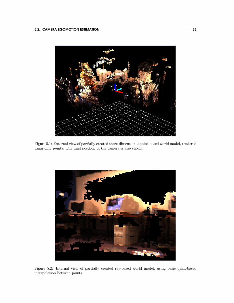
5.1 External view of partially created three-dimensional point-based world model, ren-dered using only points. The final position of the camera is also shown. . . . . . . 33

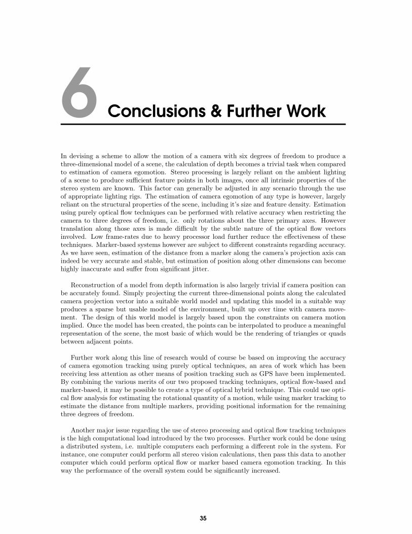
5.2 Internal view of partially created ray-based world model, using basic quad-basedinterpolation between points. . . . . . . . . . . . . . . . . . . . . . . . . . . . . . . 33

5.3 Alternative view of partially created ray-based world model, on the left showing theeffect of perpendicular view of interpolation between points. The final position ofthe camera is also shown. . . . . . . . . . . . . . . . . . . . . . . . . . . . . . . . . 34

Publications

Brendon Kelly and Richard Green. Camera Egomotion Tracking using Markers. Image and VisionComputing New Zealand, 2006.1

1Full paper published in proceedings.

vii

1 Introduction

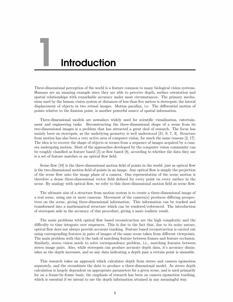
Three-dimensional perception of the world is a feature common to many biological vision systems.Humans are an amazing example since they are able to perceive depth, surface orientation andspatial relationships with remarkable accuracy under most circumstances. The primary mecha-nism used by the human vision system at distances of less than five metres is stereopsis; the lateraldisplacement of objects in two retinal images. Motion parallax, i.e. The differential motion ofpoints relative to the fixation point, is another powerful source of spatial information.

Three-dimensional models are nowadays widely used for scientific visualization, entertain-ment and engineering tasks. Reconstructing the three-dimensional shape of a scene from itstwo-dimensional images is a problem that has attracted a great deal of research. The focus hasmainly been on stereopsis, as the underlying geometry is well understood [21, 9, 7, 3]. Structurefrom motion has also been a very active area of computer vision, for much the same reasons [2, 17].The idea is to recover the shape of objects or scenes from a sequence of images acquired by a cam-era undergoing motion. Most of the approaches developed by the computer vision community canbe roughly classified as feature based [5] or flow based [8], according to whether the data they useis a set of feature matches or an optical flow field.

Scene flow [19] is the three-dimensional motion field of points in the world, just as optical flowis the two-dimensional motion field of points in an image. Any optical flow is simply the projectionof the scene flow onto the image plane of a camera. One representation of the scene motion istherefore a dense three-dimensional vector field defined for every point on every surface in thescene. By analogy with optical flow, we refer to this three-dimensional motion field as scene flow.

The ultimate aim of a structure from motion system is to create a three-dimensional image ofa real scene, using one or more cameras. Movement of the camera(s) produces differing perspec-tives on the scene, giving three-dimensional information. This information can be tracked andtransformed into a mathematical structure which can be rendered/referenced. The introductionof stereopsis aids in the accuracy of this procedure, giving a more realistic result.

The main problems with optical flow based reconstruction are the high complexity and thedifficulty to time integrate over sequences. This is due to the fact that, due to its noisy nature,optical flow does not always provide accurate tracking. Feature based reconstruction is carried outusing corresponding features in pairs of images of the same scene taken from different viewpoints.The main problem with this is the task of matching feature between frames and feature occlusion.Similarly, stereo vision needs to solve correspondence problem, i.e., matching features betweenstereo image pairs. Also, while stereopsis can produce accurate depth data, it’s accuracy dimin-ishes as the depth increases, and so any data indicating a depth past a certain point is unusable.

This research takes an approach which calculates depth from stereo and camera egomotionseparately, and the recombines the data to produce a three-dimensional model. As stereo depthcalculation is largely dependent on appropriate parameters for a given scene, and is used primarilyfor on a frame-by-frame basis, the emphasis of research has been on camera egomotion tracking,which is essential if we intend to use the depth information attained in any meaningful way.

1

2 CHAPTER 1. INTRODUCTION

2 Background & Related Work

2.1 Stereo VisionThe fundamental idea behind stereo computer vision is the difference in position of a unique pointin two different images. When a distant object is viewed by two cameras positioned in the sameorientation but separated by a known distance (baseline), that object will appear in a similarposition in both images. As the object moves closer to the camera(s), the relative position ofobject will change, and the positions in each image will move away from each other. In this way,we can calculate the distance of an object, by calculating its relative positioning in the two images.This distance between the same object in two images us known as disparity; a greater disparitymeans a closer object, and lesser disparity (or none at all) means an object further away. Themost challenging part of this process is the correlation between points in two images. If each pointin one image cannot be uniquely identified and matched to the corresponding point in the otherimage, then a disparity calculation for that point cannot be made. Once all possible disparities arecalculated, a disparity map can be created. A second task that a stereo system must undertake isthree-dimensional reconstruction of the scene. If the geometry of the stereo system is known, thedisparity map can be used to build a three-dimensional map of the current scene.

2.1.1 Simple Stereo

Figure 2.1 illustrates a top down view of a simple stereo vision system consisting of two pinholecameras. Cl and Cr represent the left and right centres of projection, while Il and Ir represent theleft and right image planes. The distance T, between the two centers of projection Cl and Cr isthe baseline of the system. A and B represent two separate points in space. A stereo system usestriangulation to determine the position of points A and B, by intersecting the rays defined by thecentres of projection and the images of A and B. This of course relies on correct correspondenceof the points in the two images.

If we take Xl and Xr to be the coordinates of Al and Ar with respect to the centre of theimage plane, f to be the common focal length of the cameras, and Z to be the distance between Aand the baseline, we can construct the following equation:

T + Xl −Xr

Z − f=

T

Z(2.1)

from which we can obtain:

Z = fT

d(2.2)

where d is Xr −Xl, or the disparity of the point in the two images.

The same calculations can be made for point B, using our simplified depth equation. Therelationship between each point and respective disparity can be seen in figure 2.2. Again Il and Ir

represent our left and right image planes, but are aligned to show the relative positions of pointsAl, Ar, Bl,and Br. As is clearly shown, the disparity dA for point A is greater than dB , thedisparity for point B, indicating that point A is closer to the baseline that point B.

3

4 CHAPTER 2. BACKGROUND & RELATED WORK

Figure 2.1: A simple stereo system.

Figure 2.2: Comparing the disparities of points A and B in the two image planes.

2.2. OPTICAL FLOW 5

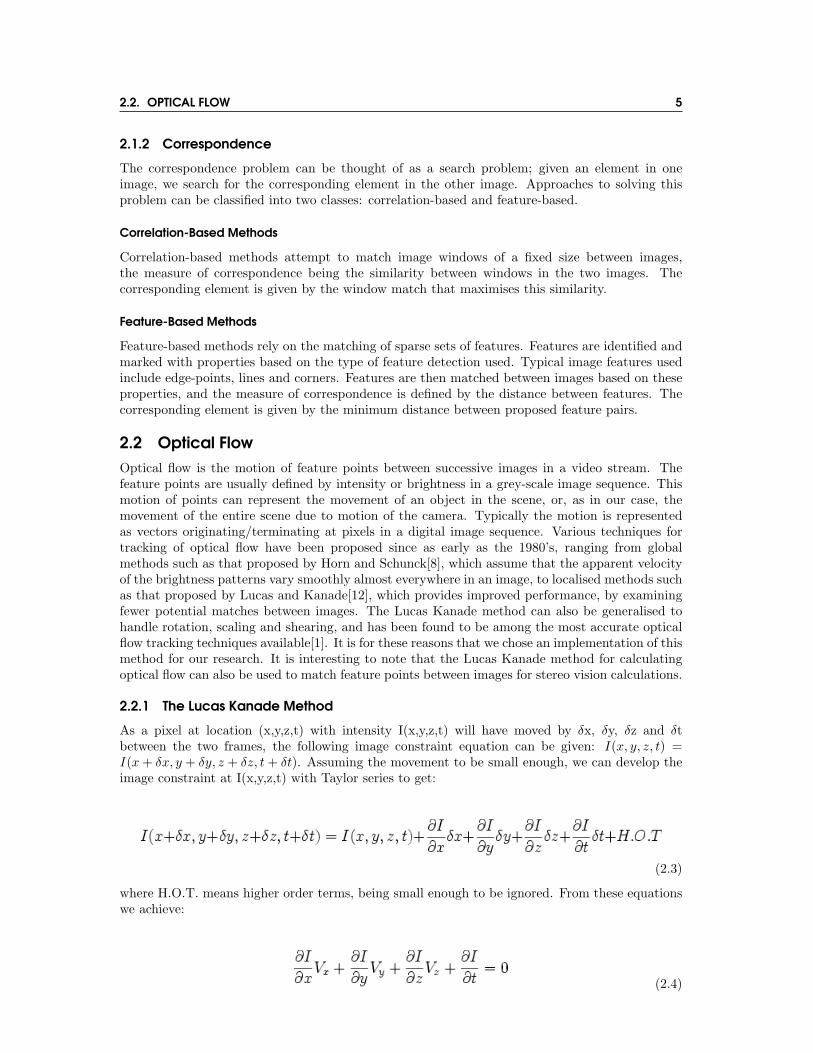
2.1.2 Correspondence

The correspondence problem can be thought of as a search problem; given an element in oneimage, we search for the corresponding element in the other image. Approaches to solving thisproblem can be classified into two classes: correlation-based and feature-based.

Correlation-Based Methods

Correlation-based methods attempt to match image windows of a fixed size between images,the measure of correspondence being the similarity between windows in the two images. Thecorresponding element is given by the window match that maximises this similarity.

Feature-Based Methods

Feature-based methods rely on the matching of sparse sets of features. Features are identified andmarked with properties based on the type of feature detection used. Typical image features usedinclude edge-points, lines and corners. Features are then matched between images based on theseproperties, and the measure of correspondence is defined by the distance between features. Thecorresponding element is given by the minimum distance between proposed feature pairs.

2.2 Optical FlowOptical flow is the motion of feature points between successive images in a video stream. Thefeature points are usually defined by intensity or brightness in a grey-scale image sequence. Thismotion of points can represent the movement of an object in the scene, or, as in our case, themovement of the entire scene due to motion of the camera. Typically the motion is representedas vectors originating/terminating at pixels in a digital image sequence. Various techniques fortracking of optical flow have been proposed since as early as the 1980’s, ranging from globalmethods such as that proposed by Horn and Schunck[8], which assume that the apparent velocityof the brightness patterns vary smoothly almost everywhere in an image, to localised methods suchas that proposed by Lucas and Kanade[12], which provides improved performance, by examiningfewer potential matches between images. The Lucas Kanade method can also be generalised tohandle rotation, scaling and shearing, and has been found to be among the most accurate opticalflow tracking techniques available[1]. It is for these reasons that we chose an implementation of thismethod for our research. It is interesting to note that the Lucas Kanade method for calculatingoptical flow can also be used to match feature points between images for stereo vision calculations.

2.2.1 The Lucas Kanade Method

As a pixel at location (x,y,z,t) with intensity I(x,y,z,t) will have moved by δx, δy, δz and δtbetween the two frames, the following image constraint equation can be given: I(x, y, z, t) =I(x + δx, y + δy, z + δz, t + δt). Assuming the movement to be small enough, we can develop theimage constraint at I(x,y,z,t) with Taylor series to get:

(2.3)

where H.O.T. means higher order terms, being small enough to be ignored. From these equationswe achieve:

(2.4)


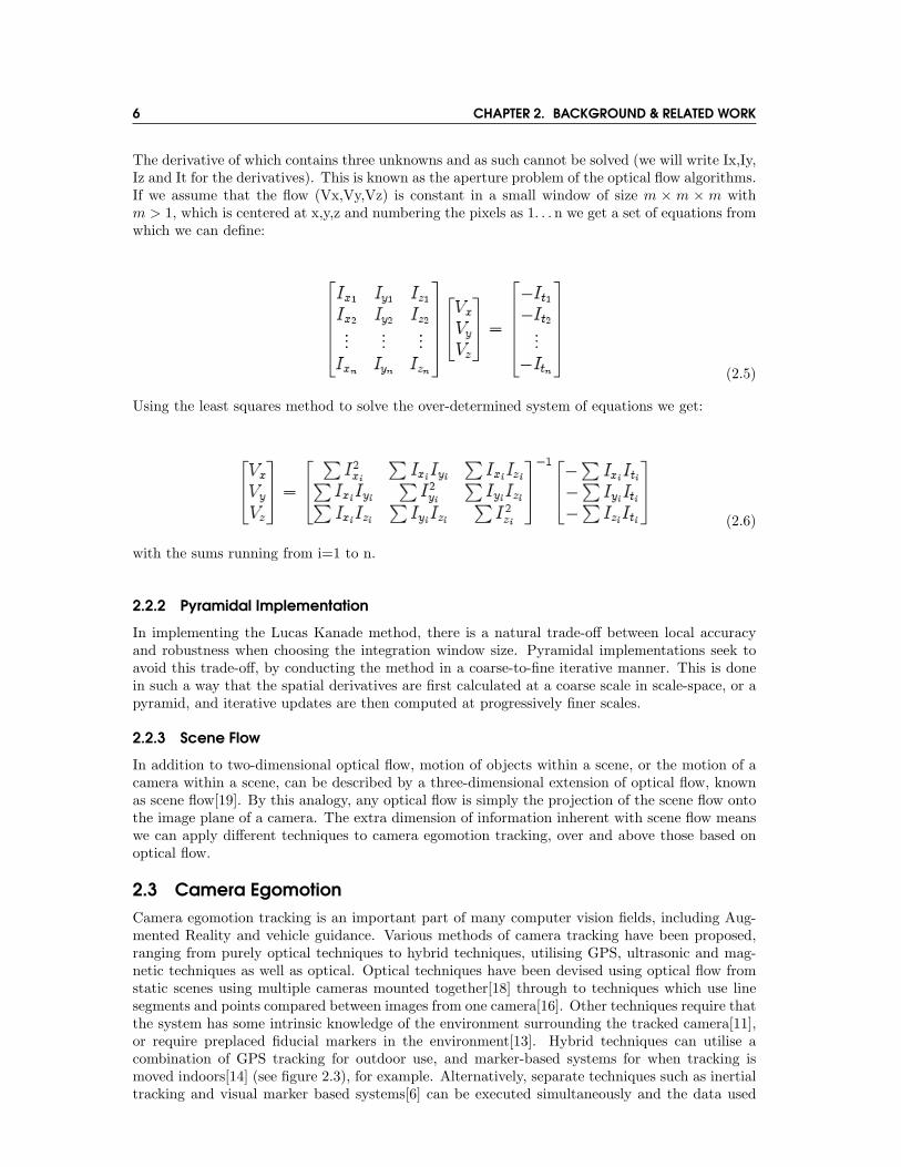
The derivative of which contains three unknowns and as such cannot be solved (we will write Ix,Iy,Iz and It for the derivatives). This is known as the aperture problem of the optical flow algorithms.If we assume that the flow (Vx,Vy,Vz) is constant in a small window of size m × m × m withm > 1, which is centered at x,y,z and numbering the pixels as 1. . . n we get a set of equations fromwhich we can define:

(2.5)

Using the least squares method to solve the over-determined system of equations we get:

(2.6)

with the sums running from i=1 to n.

2.2.2 Pyramidal Implementation

In implementing the Lucas Kanade method, there is a natural trade-off between local accuracyand robustness when choosing the integration window size. Pyramidal implementations seek toavoid this trade-off, by conducting the method in a coarse-to-fine iterative manner. This is donein such a way that the spatial derivatives are first calculated at a coarse scale in scale-space, or apyramid, and iterative updates are then computed at progressively finer scales.

2.2.3 Scene Flow

In addition to two-dimensional optical flow, motion of objects within a scene, or the motion of acamera within a scene, can be described by a three-dimensional extension of optical flow, knownas scene flow[19]. By this analogy, any optical flow is simply the projection of the scene flow ontothe image plane of a camera. The extra dimension of information inherent with scene flow meanswe can apply different techniques to camera egomotion tracking, over and above those based onoptical flow.

2.3 Camera EgomotionCamera egomotion tracking is an important part of many computer vision fields, including Aug-mented Reality and vehicle guidance. Various methods of camera tracking have been proposed,ranging from purely optical techniques to hybrid techniques, utilising GPS, ultrasonic and mag-netic techniques as well as optical. Optical techniques have been devised using optical flow fromstatic scenes using multiple cameras mounted together[18] through to techniques which use linesegments and points compared between images from one camera[16]. Other techniques require thatthe system has some intrinsic knowledge of the environment surrounding the tracked camera[11],or require preplaced fiducial markers in the environment[13]. Hybrid techniques can utilise acombination of GPS tracking for outdoor use, and marker-based systems for when tracking ismoved indoors[14] (see figure 2.3), for example. Alternatively, separate techniques such as inertialtracking and visual marker based systems[6] can be executed simultaneously and the data used

2.3. CAMERA EGOMOTION 7

Figure 2.3: Hardware configuration with three video cameras, GPS antenna, and fiducial markerson the hands and room.

to cross-calibrate and enhance the accuracy of each individual system. Our research aims to in-vestigate camera egomotion estimation techniques which utilise only one camera, and are purelyoptical-based, with either no knowledge of the environment, or using predefined marker positions.

3 Design & Implementation

3.1 Stereo Vision

Stereo vision is our chosen method of determining three-dimensional data for establishing struc-ture. By using modern stereo vision systems and algorithms, we can accurately estimate the depthof most visible structures. The Bumblebee stereo camera package from Point Grey Research formsthe basis of our stereo vision research system.

3.1.1 The PTGrey Bumblebee

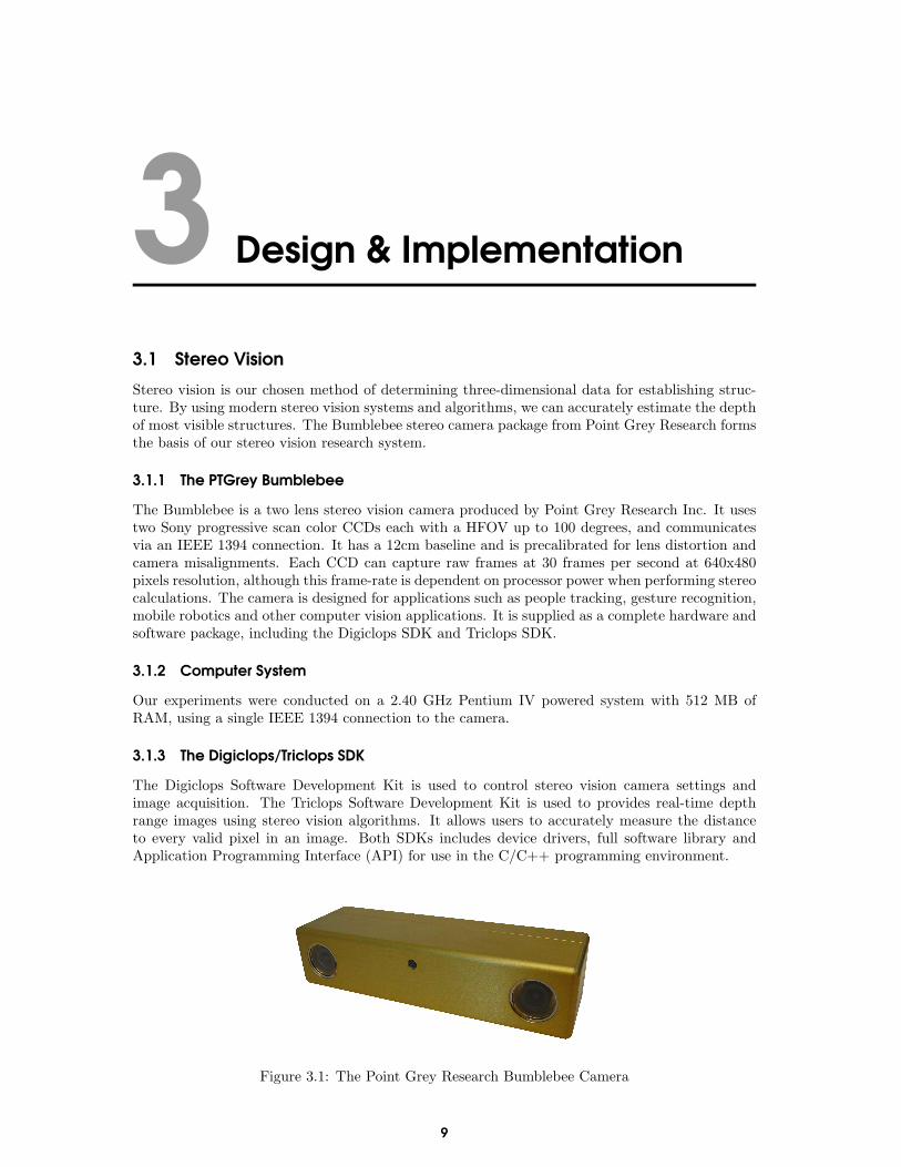
The Bumblebee is a two lens stereo vision camera produced by Point Grey Research Inc. It usestwo Sony progressive scan color CCDs each with a HFOV up to 100 degrees, and communicatesvia an IEEE 1394 connection. It has a 12cm baseline and is precalibrated for lens distortion andcamera misalignments. Each CCD can capture raw frames at 30 frames per second at 640x480pixels resolution, although this frame-rate is dependent on processor power when performing stereocalculations. The camera is designed for applications such as people tracking, gesture recognition,mobile robotics and other computer vision applications. It is supplied as a complete hardware andsoftware package, including the Digiclops SDK and Triclops SDK.

3.1.2 Computer System

Our experiments were conducted on a 2.40 GHz Pentium IV powered system with 512 MB ofRAM, using a single IEEE 1394 connection to the camera.

3.1.3 The Digiclops/Triclops SDK

The Digiclops Software Development Kit is used to control stereo vision camera settings andimage acquisition. The Triclops Software Development Kit is used to provides real-time depthrange images using stereo vision algorithms. It allows users to accurately measure the distanceto every valid pixel in an image. Both SDKs includes device drivers, full software library andApplication Programming Interface (API) for use in the C/C++ programming environment.

Figure 3.1: The Point Grey Research Bumblebee Camera

9

10 CHAPTER 3. DESIGN & IMPLEMENTATION

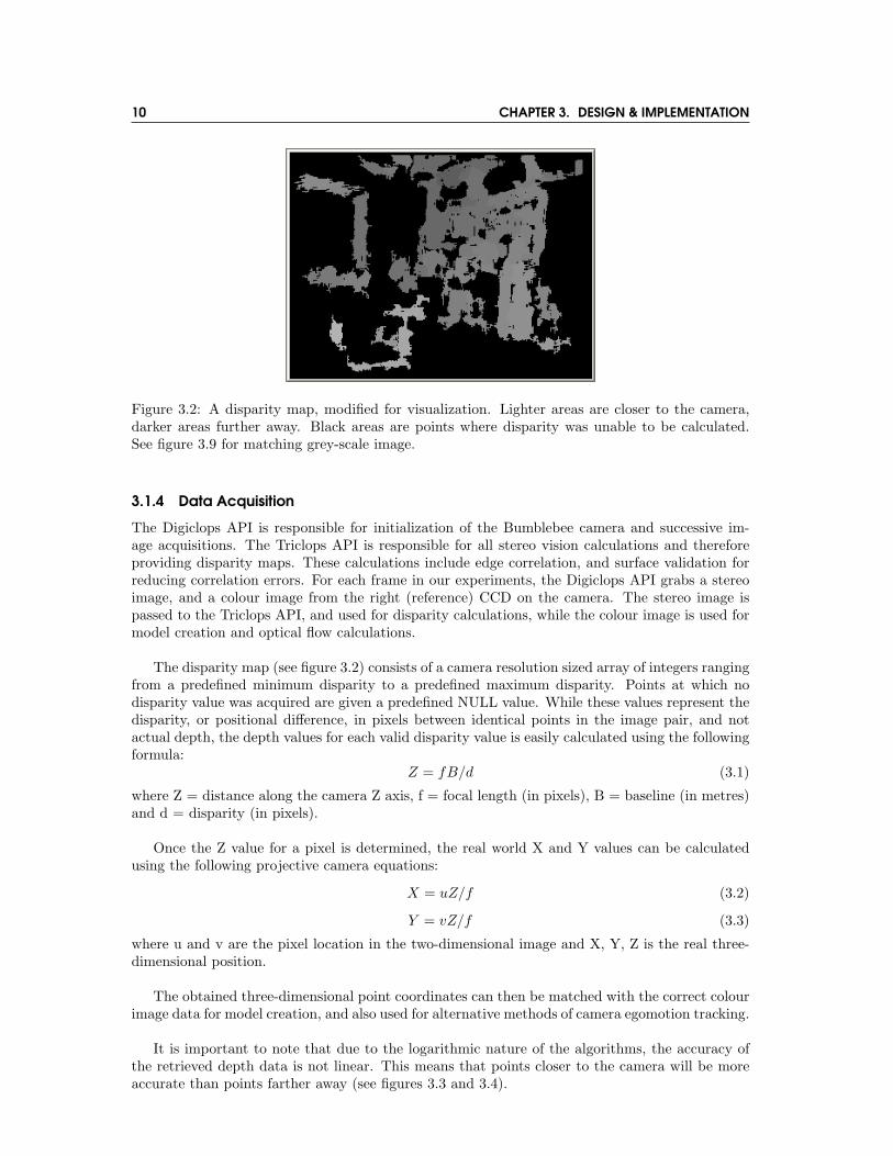
Figure 3.2: A disparity map, modified for visualization. Lighter areas are closer to the camera,darker areas further away. Black areas are points where disparity was unable to be calculated.See figure 3.9 for matching grey-scale image.

3.1.4 Data Acquisition

The Digiclops API is responsible for initialization of the Bumblebee camera and successive im-age acquisitions. The Triclops API is responsible for all stereo vision calculations and thereforeproviding disparity maps. These calculations include edge correlation, and surface validation forreducing correlation errors. For each frame in our experiments, the Digiclops API grabs a stereoimage, and a colour image from the right (reference) CCD on the camera. The stereo image ispassed to the Triclops API, and used for disparity calculations, while the colour image is used formodel creation and optical flow calculations.

The disparity map (see figure 3.2) consists of a camera resolution sized array of integers rangingfrom a predefined minimum disparity to a predefined maximum disparity. Points at which nodisparity value was acquired are given a predefined NULL value. While these values represent thedisparity, or positional difference, in pixels between identical points in the image pair, and notactual depth, the depth values for each valid disparity value is easily calculated using the followingformula:

Z = fB/d (3.1)

where Z = distance along the camera Z axis, f = focal length (in pixels), B = baseline (in metres)and d = disparity (in pixels).

Once the Z value for a pixel is determined, the real world X and Y values can be calculatedusing the following projective camera equations:

X = uZ/f (3.2)

Y = vZ/f (3.3)

where u and v are the pixel location in the two-dimensional image and X, Y, Z is the real three-dimensional position.

The obtained three-dimensional point coordinates can then be matched with the correct colourimage data for model creation, and also used for alternative methods of camera egomotion tracking.

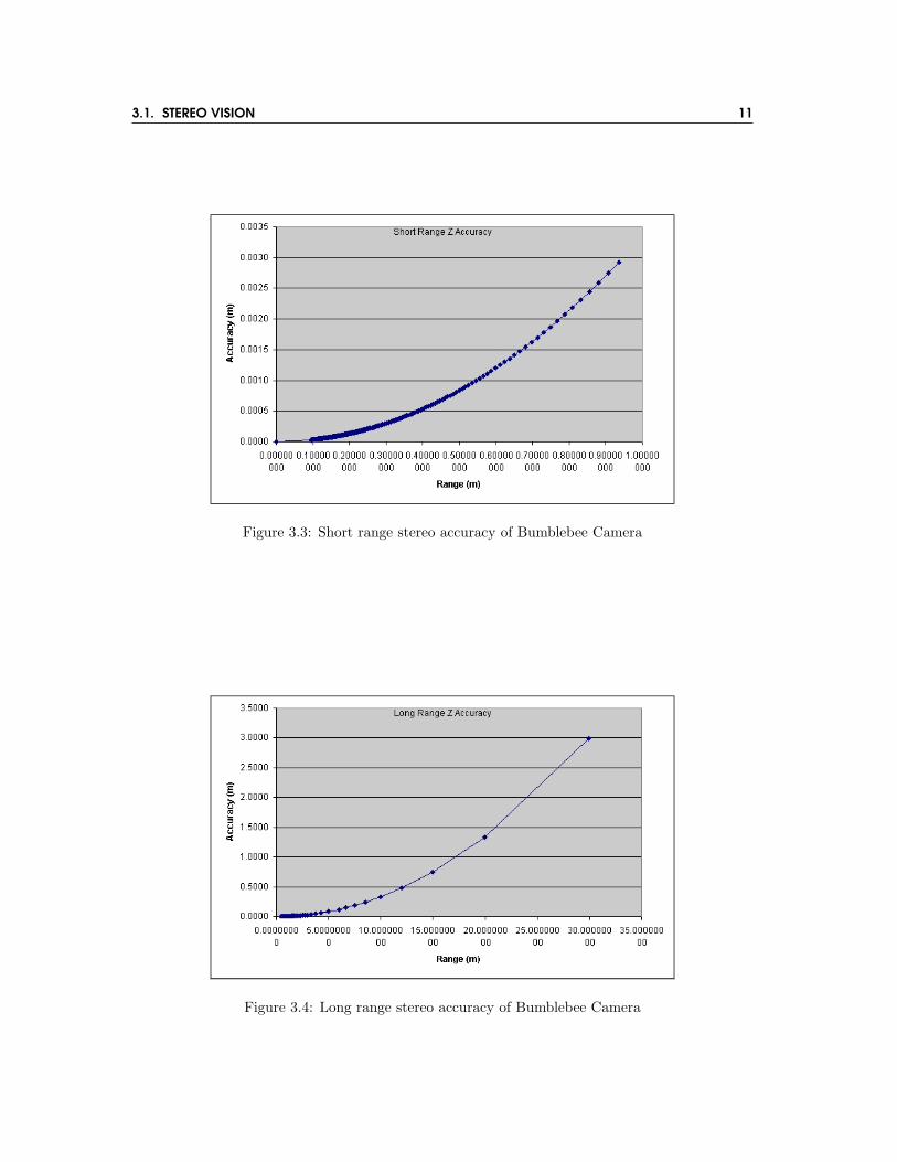
It is important to note that due to the logarithmic nature of the algorithms, the accuracy ofthe retrieved depth data is not linear. This means that points closer to the camera will be moreaccurate than points farther away (see figures 3.3 and 3.4).

3.1. STEREO VISION 11

Figure 3.3: Short range stereo accuracy of Bumblebee Camera

Figure 3.4: Long range stereo accuracy of Bumblebee Camera


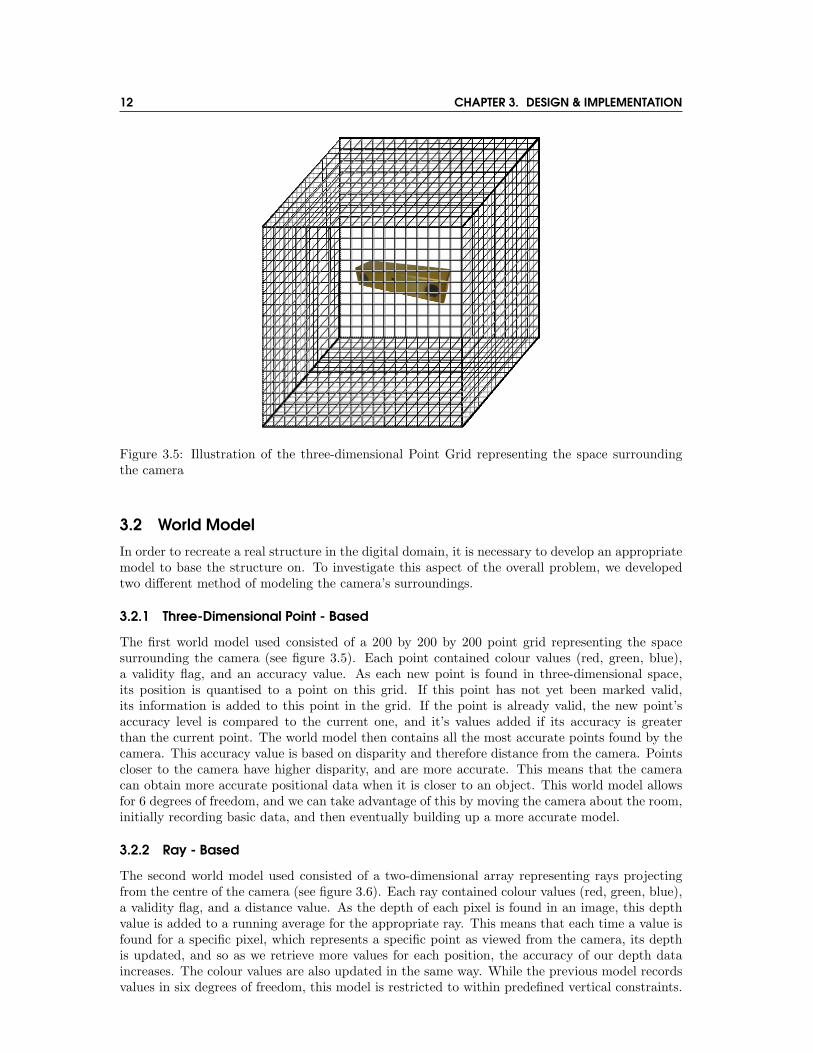
Figure 3.5: Illustration of the three-dimensional Point Grid representing the space surroundingthe camera

3.2 World Model

In order to recreate a real structure in the digital domain, it is necessary to develop an appropriatemodel to base the structure on. To investigate this aspect of the overall problem, we developedtwo different method of modeling the camera’s surroundings.

3.2.1 Three-Dimensional Point - Based

The first world model used consisted of a 200 by 200 by 200 point grid representing the spacesurrounding the camera (see figure 3.5). Each point contained colour values (red, green, blue),a validity flag, and an accuracy value. As each new point is found in three-dimensional space,its position is quantised to a point on this grid. If this point has not yet been marked valid,its information is added to this point in the grid. If the point is already valid, the new point’saccuracy level is compared to the current one, and it’s values added if its accuracy is greaterthan the current point. The world model then contains all the most accurate points found by thecamera. This accuracy value is based on disparity and therefore distance from the camera. Pointscloser to the camera have higher disparity, and are more accurate. This means that the cameracan obtain more accurate positional data when it is closer to an object. This world model allowsfor 6 degrees of freedom, and we can take advantage of this by moving the camera about the room,initially recording basic data, and then eventually building up a more accurate model.

3.2.2 Ray - Based

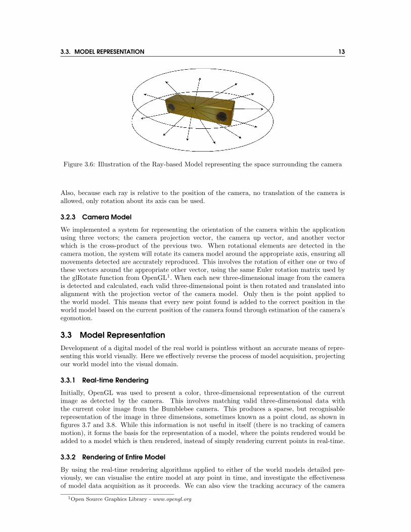
The second world model used consisted of a two-dimensional array representing rays projectingfrom the centre of the camera (see figure 3.6). Each ray contained colour values (red, green, blue),a validity flag, and a distance value. As the depth of each pixel is found in an image, this depthvalue is added to a running average for the appropriate ray. This means that each time a value isfound for a specific pixel, which represents a specific point as viewed from the camera, its depthis updated, and so as we retrieve more values for each position, the accuracy of our depth dataincreases. The colour values are also updated in the same way. While the previous model recordsvalues in six degrees of freedom, this model is restricted to within predefined vertical constraints.

3.3. MODEL REPRESENTATION 13

Figure 3.6: Illustration of the Ray-based Model representing the space surrounding the camera

Also, because each ray is relative to the position of the camera, no translation of the camera isallowed, only rotation about its axis can be used.

3.2.3 Camera Model

We implemented a system for representing the orientation of the camera within the applicationusing three vectors; the camera projection vector, the camera up vector, and another vectorwhich is the cross-product of the previous two. When rotational elements are detected in thecamera motion, the system will rotate its camera model around the appropriate axis, ensuring allmovements detected are accurately reproduced. This involves the rotation of either one or two ofthese vectors around the appropriate other vector, using the same Euler rotation matrix used bythe glRotate function from OpenGL1. When each new three-dimensional image from the camerais detected and calculated, each valid three-dimensional point is then rotated and translated intoalignment with the projection vector of the camera model. Only then is the point applied tothe world model. This means that every new point found is added to the correct position in theworld model based on the current position of the camera found through estimation of the camera’segomotion.

3.3 Model RepresentationDevelopment of a digital model of the real world is pointless without an accurate means of repre-senting this world visually. Here we effectively reverse the process of model acquisition, projectingour world model into the visual domain.

3.3.1 Real-time Rendering

Initially, OpenGL was used to present a color, three-dimensional representation of the currentimage as detected by the camera. This involves matching valid three-dimensional data withthe current color image from the Bumblebee camera. This produces a sparse, but recognisablerepresentation of the image in three dimensions, sometimes known as a point cloud, as shown infigures 3.7 and 3.8. While this information is not useful in itself (there is no tracking of cameramotion), it forms the basis for the representation of a model, where the points rendered would beadded to a model which is then rendered, instead of simply rendering current points in real-time.

3.3.2 Rendering of Entire Model

By using the real-time rendering algorithms applied to either of the world models detailed pre-viously, we can visualise the entire model at any point in time, and investigate the effectivenessof model data acquisition as it proceeds. We can also view the tracking accuracy of the camera

1Open Source Graphics Library - www.opengl.org


Figure 3.7: View of current point cloud from directly behind the camera. Camera is representedby three coloured vectors.

Figure 3.8: View of same point cloud from a position perpendicular to the camera. Due to thelogarithmic nature of the stereo equation, each successive step of disparity beyond the camera islarger than the last.

3.4. EGOMOTION TRACKING 15

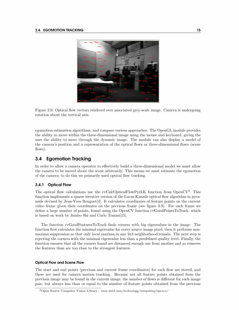
Figure 3.9: Optical flow vectors rendered over associated grey-scale image. Camera is undergoingrotation about the vertical axis.

egomotion estimation algorithms, and compare various approaches. The OpenGL module providesthe ability to move within the three-dimensional image using the mouse and keyboard, giving theuser the ability to move through the dynamic image. The module can also display a model ofthe camera’s position and a representation of the optical flows or three-dimensional flows (sceneflows).

3.4 Egomotion TrackingIn order to allow a camera operator to effectively build a three-dimensional model we must allowthe camera to be moved about the scene arbitrarily. This means we must estimate the egomotionof the camera; to do this we primarily used optical flow tracking.

3.4.1 Optical Flow

The optical flow calculations use the cvCalcOpticalFlowPyrLK function from OpenCV2. Thisfunction implements a sparse iterative version of the Lucas-Kanade optical flow algorithm in pyra-mids devised by Jean-Yves Bouguet[4]. It calculates coordinates of feature points on the currentvideo frame given their coordinates on the previous frame (see figure 3.9). For each frame wedefine a large number of points, found using the OpenCV function cvGoodPointsToTrack, whichis based on work by Jianbo Shi and Carlo Tomasi[15].

The function cvGoodFeaturesToTrack finds corners with big eigenvalues in the image. Thefunction first calculates the minimal eigenvalue for every source image pixel, then it performs non-maxima suppression so that only local maxima in any 3x3 neighborhood remain. The next step isrejecting the corners with the minimal eigenvalue less than a predefined quality level. Finally, thefunction ensures that all the corners found are distanced enough one from another and so removesthe features than are too close to the strongest features.

Optical Flow and Scene Flow

The start and end points (previous and current frame coordinates) for each flow are stored, andthese are used for camera motion tracking. Because not all feature points obtained from theprevious image may be found in the current image, the number of flows is different for each imagepair, but always less than or equal to the number of feature points obtained from the previous

2Open Source Computer Vision Library - www.intel.com/technology/computing/opencv/


Figure 3.10: Optical flow field for a camera undergoing pure rotation about the X and then Yaxes.

image. Each flows structure stores the previous and current screen coordinates, and the velocityvector associated with the coordinate pair. Each of these flow structures is then matched to thecurrent and previous disparity maps, and if both the previous and current screen coordinateshave valid depth values in the appropriate disparity map, then a scene flow structure is created,which includes Z (depth) values as well as X and Y coordinates. These scene flows can be used inaddition to optical flows to estimate camera egomotion.

Tracking Rotation Around the Camera’s X and Y Axes

Tracking rotation around the camera’s X and Y axes involves calculating the average movement ofall optical flows (two-dimensional) in consecutive images. Under x/y rotation, all flows will be ofequal magnitude, irrespective of the distance of the feature which was being tracked by the flow,as shown in figure 3.10. Therefore the average flow movement in the X directions will relate tothe angle rotated, by the formula:

camerarotationy = −avgmovementx × totalviewinganglex

resolutionx(3.4)

For example, with an X resolution of 320 pixels, a viewing angle of 90 degrees, and an averageX component movement of +6 pixels between frames, we calculate a rotation of -1.6875 degreesaround the vertical axis. The same equation is applicable when working with the Y component ofa movement, with the X and Y subscripts swapped.

Tracking Rotation Around the Camera’s Z Axis

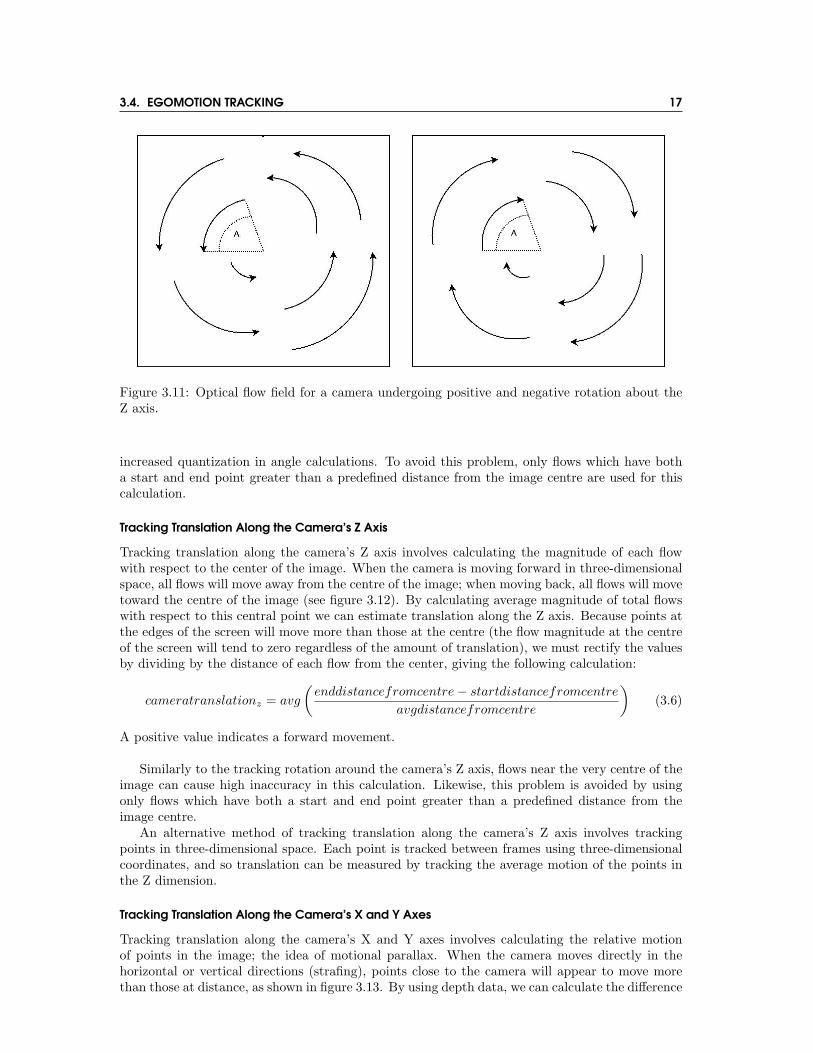
Tracking rotation around the camera’s Z axis involves calculating the average rotation of flowsaround the centre point of the image. Under pure Z rotation, the centre of the image will experienceflow of magnitude zero, while all other flows will represent a circular movement around it, as shownin figure 3.11. By finding the angle of both the start and end points of each flow, with respectto the center point, we can subtract to give the angle of rotation for each flow, the average of allflows giving the amount of rotation around the Z axis.

camerarotationz = −avg(arctan(endposition− center)− arctan(startposition− center)) (3.5)

Because of the relatively low camera resolution being used, flows near the very centre of theimage can cause high inaccuracy in this calculation, as the pixelisation of feature points causes


Figure 3.11: Optical flow field for a camera undergoing positive and negative rotation about theZ axis.

increased quantization in angle calculations. To avoid this problem, only flows which have botha start and end point greater than a predefined distance from the image centre are used for thiscalculation.

Tracking Translation Along the Camera’s Z Axis

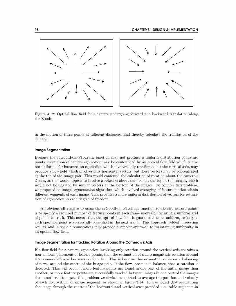
Tracking translation along the camera’s Z axis involves calculating the magnitude of each flowwith respect to the center of the image. When the camera is moving forward in three-dimensionalspace, all flows will move away from the centre of the image; when moving back, all flows will movetoward the centre of the image (see figure 3.12). By calculating average magnitude of total flowswith respect to this central point we can estimate translation along the Z axis. Because points atthe edges of the screen will move more than those at the centre (the flow magnitude at the centreof the screen will tend to zero regardless of the amount of translation), we must rectify the valuesby dividing by the distance of each flow from the center, giving the following calculation:

cameratranslationz = avg

(enddistancefromcentre− startdistancefromcentre

avgdistancefromcentre

)(3.6)

A positive value indicates a forward movement.

Similarly to the tracking rotation around the camera’s Z axis, flows near the very centre of theimage can cause high inaccuracy in this calculation. Likewise, this problem is avoided by usingonly flows which have both a start and end point greater than a predefined distance from theimage centre.

An alternative method of tracking translation along the camera’s Z axis involves trackingpoints in three-dimensional space. Each point is tracked between frames using three-dimensionalcoordinates, and so translation can be measured by tracking the average motion of the points inthe Z dimension.

Tracking Translation Along the Camera’s X and Y Axes

Tracking translation along the camera’s X and Y axes involves calculating the relative motionof points in the image; the idea of motional parallax. When the camera moves directly in thehorizontal or vertical directions (strafing), points close to the camera will appear to move morethan those at distance, as shown in figure 3.13. By using depth data, we can calculate the difference


Figure 3.12: Optical flow field for a camera undergoing forward and backward translation alongthe Z axis.

in the motion of these points at different distances, and thereby calculate the translation of thecamera:

Image Segmentation

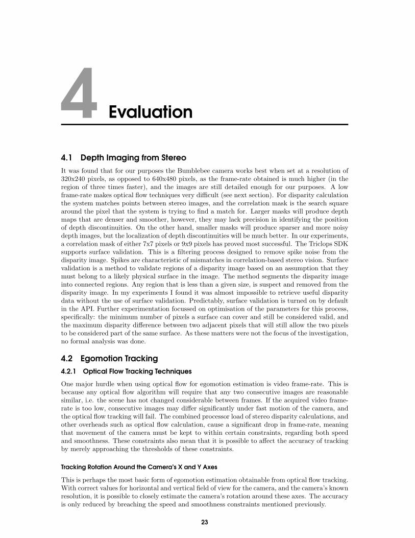
Because the cvGoodPointsToTrack function may not produce a uniform distribution of featurepoints, estimation of camera egomotion may be confounded by an optical flow field which is alsonot uniform. For instance, an egomotion which involves only rotation about the vertical axis, mayproduce a flow field which involves only horizontal vectors, but these vectors may be concentratedat the top of the image pair. This would confound the calculation of rotation about the camera’sZ axis, as this would appear to involve a rotation about this axis at the top of the images, whichwould not be negated by similar vectors at the bottom of the images. To counter this problem,we proposed an image segmentation algorithm, which involved averaging of feature motion withindifferent segments of each image. This provides a more uniform distribution of vectors for estima-tion of egomotion in each degree of freedom.

An obvious alternative to using the cvGoodPointsToTrack function to identify feature pointsis to specify a required number of feature points in each frame manually, by using a uniform gridof points to track. This means that the optical flow field is guaranteed to be uniform, as long aseach specified point is successfully identified in the next frame. This approach yielded interestingresults, and in some circumstances may provide a simpler approach to maintaining uniformity inan optical flow field.

Image Segmentation for Tracking Rotation Around the Camera’s Z Axis

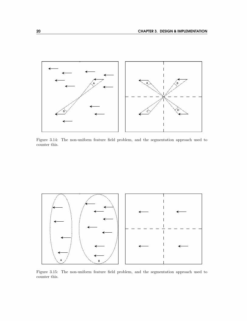
If a flow field for a camera egomotion involving only rotation around the vertical axis contains anon-uniform placement of feature points, then the estimation of a zero magnitude rotation aroundthat camera’s Z axis becomes confounded. This is because this estimation relies on a balancingof flows, around the centre of the image pair. If the flows are not in balance, then a rotation isdetected. This will occur if more feature points are found in one part of the initial image thananother, or more feature points are successfully tracked between images in one part of the imagesthan another. To negate this problem we devised a method to average the position and velocityof each flow within an image segment, as shown in figure 3.14. It was found that segmentingthe image through the centre of the horizontal and vertical axes provided 4 suitable segments in


Figure 3.13: Optical flow field for a camera undergoing translation along the X axis, and simulatedvertical view of flows. Flows of greater magnitude are those closer than those of smaller magnitude.

which to perform averaging. This allows the algorithm to attain accurate results regardless of theuniformity of the initial feature field found.

Image Segmentation for Tracking Translation Along the Camera’s Z Axis

A similar problem occurs when estimating the forward/backward egomotion of the camera, i.e.along the camera’s Z axis. Under pure forward translation, with a uniform optical flow field, allflows will point away from the centre of the image pair, with a similar velocity proportional totheir distance from the centre of the image pair. Therefore we can take the average of these values,and from this estimate the forward translation. If, however, we have a rotation about the verticalaxis, with a non-uniform distribution, the calculation may become unbalanced, as a the number offlows directed toward the centre of the image pair may not be balanced by those directed away. Tonegate this problem we devised a segmentation method similar to that detailed previously, usingan average flow velocity value for each image segment, allowing accurate results regardless of theuniformity of the feature field found in the first image (see figure 3.15).

3.4.2 Marker-Based Tracking

In addition to optical flow tracking, the performance of camera egomotion tracking using fixedmarkers was investigated. Tracking was performed using two different marker-based tracking sys-tems. We also investigated the feasibility of using multiple markers for camera egomotion tracking,and proposed a novel algorithm which can be used to devise the most efficient marker placementstrategy for use with a multiple-marker based camera egomotion tracking system.

The ARToolKit[10] system is generally used to find the 6DOF position of markers relative to acamera, and therefore if these markers are fixed, we can use ARToolKit in reverse, by inverting thematrix used to represent each marker. This gives us a 6DOF position for the camera, with respectto a marker, whose position we already know. This inversion of the matrix of course, can causehigh levels of tracking error at greater distances. We also used a second augmented reality system,ARToolKitPlus[20], which was, in part, developed to improve the tracking abilities of ARToolKit.It uses similar markers to ARToolKit, but markers require no training, as the marker identifieris embedded in the pattern itself. ARToolKitPlus is an extended version of ARToolKit’s visioncode that adds new features, but breaks compatibility due to its class-based API. The extensionsmade in ARToolKitPlus include implementation of the Robust Planar Pose (RPP) algorithm. The


Figure 3.14: The non-uniform feature field problem, and the segmentation approach used tocounter this.

Figure 3.15: The non-uniform feature field problem, and the segmentation approach used tocounter this.


Figure 3.16: Multiple ARToolKit markers being used for camera tracking.

RPP algorithm is used to give a more stable tracking than ARToolKit’s pose estimation algorithm.

Further to this, we investigated the efficient use of multiple markers at once to calculate cameraposition, as shown in figure 3.16. The hypothesis here is that the greater the number of markers,the greater the reduction in error that may be induced by the large distances we intend to trackover.

Finally, we introduced a novel algorithm to determine appropriate placement of ARToolKitstyle markers for camera tracking. This is important, as a layout which is too sparse will meanthe camera can move to positions where no markers are visible, and a layout which is too densewill be impractical, and cause significant visual pollution of the work space.

4 Evaluation

4.1 Depth Imaging from StereoIt was found that for our purposes the Bumblebee camera works best when set at a resolution of320x240 pixels, as opposed to 640x480 pixels, as the frame-rate obtained is much higher (in theregion of three times faster), and the images are still detailed enough for our purposes. A lowframe-rate makes optical flow techniques very difficult (see next section). For disparity calculationthe system matches points between stereo images, and the correlation mask is the search squarearound the pixel that the system is trying to find a match for. Larger masks will produce depthmaps that are denser and smoother, however, they may lack precision in identifying the positionof depth discontinuities. On the other hand, smaller masks will produce sparser and more noisydepth images, but the localization of depth discontinuities will be much better. In our experiments,a correlation mask of either 7x7 pixels or 9x9 pixels has proved most successful. The Triclops SDKsupports surface validation. This is a filtering process designed to remove spike noise from thedisparity image. Spikes are characteristic of mismatches in correlation-based stereo vision. Surfacevalidation is a method to validate regions of a disparity image based on an assumption that theymust belong to a likely physical surface in the image. The method segments the disparity imageinto connected regions. Any region that is less than a given size, is suspect and removed from thedisparity image. In my experiments I found it was almost impossible to retrieve useful disparitydata without the use of surface validation. Predictably, surface validation is turned on by defaultin the API. Further experimentation focussed on optimisation of the parameters for this process,specifically: the minimum number of pixels a surface can cover and still be considered valid, andthe maximum disparity difference between two adjacent pixels that will still allow the two pixelsto be considered part of the same surface. As these matters were not the focus of the investigation,no formal analysis was done.

4.2 Egomotion Tracking4.2.1 Optical Flow Tracking Techniques

One major hurdle when using optical flow for egomotion estimation is video frame-rate. This isbecause any optical flow algorithm will require that any two consecutive images are reasonablesimilar, i.e. the scene has not changed considerable between frames. If the acquired video frame-rate is too low, consecutive images may differ significantly under fast motion of the camera, andthe optical flow tracking will fail. The combined processor load of stereo disparity calculations, andother overheads such as optical flow calculation, cause a significant drop in frame-rate, meaningthat movement of the camera must be kept to within certain constraints, regarding both speedand smoothness. These constraints also mean that it is possible to affect the accuracy of trackingby merely approaching the thresholds of these constraints.

Tracking Rotation Around the Camera’s X and Y Axes

This is perhaps the most basic form of egomotion estimation obtainable from optical flow tracking.With correct values for horizontal and vertical field of view for the camera, and the camera’s knownresolution, it is possible to closely estimate the camera’s rotation around these axes. The accuracyis only reduced by breaching the speed and smoothness constraints mentioned previously.

23

24 CHAPTER 4. EVALUATION

Tracking Rotation Around the Camera’s Z Axis

Tracking rotation around the camera’s Z axis is similarly trivial to obtain, regardless of the cam-era’s resolution and field of view. Only an accurately rectified sequence of images is required, i.e.any fish-eye effect has been satisfactorily rectified. Under pure rotation around the Z axis evenspeed and smoothness constraints are not as important, as the magnitude of each flow is not aslarge. As mentioned previously estimation of this element of rotation can be confounded by si-multaneous rotation around other axes, but this problem has been minimised by our segmentationapproach (see next section).

Tracking Translation Along the Camera’s Z Axis

Tracking translation along the camera’s Z axis poses a more difficult challenge, because of twomain factors:

• The average magnitude of flows toward/away from the centre of the image pair is very small,even under significant forward/backward translation.

• The magnitude of these flows is dependent on the distance of feature points. If all recognisedfeature points are at a significant distance from the camera, then any detected flows will beof virtually zero magnitude, providing no usable information.

The combination of these two problems means that tracking this kind of camera egomotion usingoptical flow is virtually impossible. While an increase in camera resolution may provide the abil-ity to more accurately identify feature point motion, an environment with no close range featurepoints will still provide little information regarding forward/backward translation.

An alternative method of estimating this translation was investigated, using the motion offeature points in three dimensions, i.e. scene flow. While this appeared to give slightly morefavourable results, a similar problem regarding feature distance was found, although for differentreasons. As mentioned previously, stereo depth calculations result in a error rate which is non-linear; points further away will give greater error than those close to the camera. This meansthat when tracking translation using this method, a significant number of close feature pointsare required to maintain smooth motion estimation. If nearby feature points are not present, theresolution of motion estimation is increased to a point where tracking is not viable. Thereforethis method of tracking, while an improvement over a purely optical flow based technique, is notviable for the type of camera egomotion estimation we require.

Tracking Translation Along the Camera’s X and Y Axes

Tracking translation along the camera’s X and Y axes is certainly the most difficult aspect ofegomotion to estimate using visual techniques, as it suffers from the same inherent problems asthe tracking translation along the camera’s Z axis (lack of flow magnitude and the need for closerange feature points), and also requires the tracking of feature points in all three dimensions.In our experiments regarding this type of motion, it was found that any attempt to detect thistype of translation was highly unstable even under ideal conditions, and significantly affected byother forms of motion, particularly rotation around the camera’s same axes. While this form oftranslation was not investigated as fully as we would have liked, it is unlikely that any estimationmethodology will provide an accurate form of tracking using visual techniques alone.

4.2.2 Image Segmentation

Our image segmentation approach provided a simple yet effective solution to a problem inherentwithin the tracking of optical flow fields.


Figure 4.1: Results of experiment comparing raw calculation of rotation around Z axis, to oursegmentation approach.

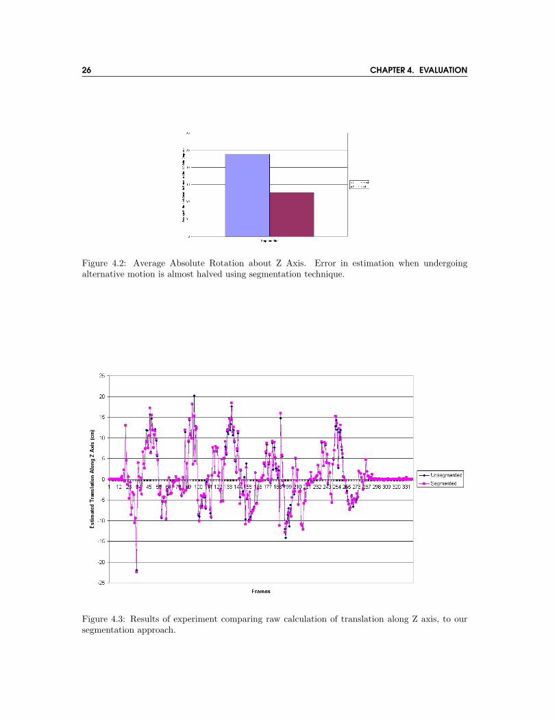
Image Segmentation for Tracking Rotation Around the Camera’s Z Axis

Experiments showed that our technique for image segmentation for tracking rotation around thecamera’s Z axis resulted in an approximate halving in the error caused by non-uniform fields ofoptical flow. Experiments were conducted calculating the rotation around the camera’s Z axis asthe camera was arbitrarily rotated about an alternative axis, in this case the Y (vertical) axis.Under these circumstances the rotation around the Z axis for each frame should be zero, but asdetailed previously this does not always occur. Figure 4.1 shows the rotation estimation for eachof a series of frames, for both raw rotation information, and our segmented results. As shown hereand in figure 4.2, a significant performance gain was attained.

Image Segmentation for Tracking Translation Along the Camera’s Z Axis

Experiments regarding image segmentation for tracking translation along the camera’s Z axisshowed less promising results. As for the last experiment, calculations were made as the camerawas rotated about the Y axis. Under these circumstances the translation along the Z axis foreach frame should also be zero. Figure 4.3 shows there appeared to be no significant advantagein using our segmentation technique when performing this motion estimation. The inaccuracy inestimating this type of motion is also clearly apparent.

4.2.3 Feature Point Grid

A second approach devised to reduce reliance on image segmentation using a predefined grid offeature points was found to be viable under some circumstances, but not robust enough to usepractically. Because these points were specified based to their position in an image, and not theirfeature strength, they were difficult to track using our optical flow algorithm. Typically, pointswere not able to be tracked between frames, or tracked very inaccurately (similar points wereconfused between frame). This inaccuracy caused more point tracking problems than could be


Figure 4.2: Average Absolute Rotation about Z Axis. Error in estimation when undergoingalternative motion is almost halved using segmentation technique.

Figure 4.3: Results of experiment comparing raw calculation of translation along Z axis, to oursegmentation approach.


reasonably tolerated, and provided poor tracking stability when used for motion estimation.

4.2.4 Marker-based Tracking

The experiments conducted to evaluate the performance of our tracking systems consist of a seriesof accuracy and stability tests conducted using a webcam moving about a room. The room mea-sures 6.6m by 5.5m by 3.0m and markers of size 20cm by 20cm are positioned at various pointson the walls. Although bigger markers will provide greater accuracy and range for our system,we have constrained the marker size to be within the bounds of a standard A4 piece of paper,to ensure ease of marker creation. A single, standard webcam is used, running at a resolution of640x480 pixels.

Our multiple marker experiments used the ARToolKit system, with two markers positionedon a 5.50m long by 3.0m high wall. The markers were both positioned at 1.5 m high, each 1/3(1.83m) of the way from the end of the walls. The camera was positioned at a height of 1.25m,directly in line with the a point bisecting the two markers. The application developed for theseexperiments provided position values in millimetres, relative to the very centre of the room, atfloor level. This meant that our first position was at X = 0, Y = 1250, Z = 1000. This was theclosest we could get the camera, while still being able to identify both markers. In each subsequentrecording we decreased the Z distance by 0.5 metres, until marker tracking was no longer achieved.At each position, 1000 calculated position values were taken. To analyse results, we calculatedthe mean value returned to measure accuracy, and the standard deviation in returned values tomeasure jitter.

Our ARToolKit vs ARToolKitPlus experiments were performed with a single marker placedat the central position of a 5.5m by 3m wall. The camera was positioned at a height of 1.25m,directly in line with the marker. The application developed for these experiments provided po-sition values in millimetres, relative to the very centre of the room, at floor level. This meantthat our first position was at X = 0, Y = 1250, Z = 2000. In each subsequent recording wedecreased the Z distance by 0.5 metres, until marker tracking was no longer achieved. At eachposition, 1000 calculated position values were taken. To analyse results, we calculated the meanvalue returned to measure accuracy, and the standard deviation in returned values to measurejitter. The only change required between ARToolKit and ARToolKitPlus experiments was theuse of a different marker, which was positioned in exactly the same place. Two settings wereused when evaluating ARToolKitPlus; one using the standard ARToolKit pose estimator, and oneusing the RPP algorithm included with ARToolKitPlus. Thresholding of the camera image is animportant part of marker detection in both ARToolKit and ARToolKitPlus. When conductingARToolKitPlus experiments, its automatic thresholding feature was used. As ARToolKit does nothave an automatic thresholding feature, this threshold was manually set.

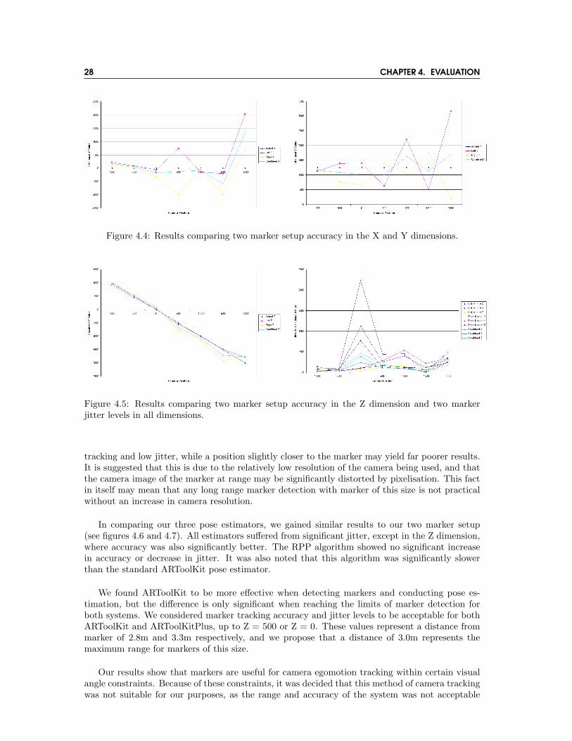
Initial investigation into the performance of ARToolKit for camera position tracking showeda drop in tracking performance once distance from the marker exceeded 2m. Tracking becamesignificantly less accurate, with a large amount of jitter, as shown in figures 4.4 and 4.5. Thisjitter was also dependent on the camera’s relative positive with regard to the marker, so at somepositions the estimation was stable, at others it was highly unstable. This was clearly evidentwhen using more than one marker for position estimation. When using two markers, one would befar more stable than the other, but this relationship could be inverted by only a small change incamera position. This jitter was most evident in the X and Y values, while the Z values (distancefrom marker), showed significantly less jitter. These Z values were also far more accurate at rangethan values in the other two dimensions.

It is important to note that the accuracy and jitter levels for position calculation do not share alinear relationship with marker range. Once the size of the marker in the camera image, sometimesknown as the visual angle, drops below a certain threshold, certain positions will yield accurate


Figure 4.4: Results comparing two marker setup accuracy in the X and Y dimensions.

Figure 4.5: Results comparing two marker setup accuracy in the Z dimension and two markerjitter levels in all dimensions.

tracking and low jitter, while a position slightly closer to the marker may yield far poorer results.It is suggested that this is due to the relatively low resolution of the camera being used, and thatthe camera image of the marker at range may be significantly distorted by pixelisation. This factin itself may mean that any long range marker detection with marker of this size is not practicalwithout an increase in camera resolution.

In comparing our three pose estimators, we gained similar results to our two marker setup(see figures 4.6 and 4.7). All estimators suffered from significant jitter, except in the Z dimension,where accuracy was also significantly better. The RPP algorithm showed no significant increasein accuracy or decrease in jitter. It was also noted that this algorithm was significantly slowerthan the standard ARToolKit pose estimator.

We found ARToolKit to be more effective when detecting markers and conducting pose es-timation, but the difference is only significant when reaching the limits of marker detection forboth systems. We considered marker tracking accuracy and jitter levels to be acceptable for bothARToolKit and ARToolKitPlus, up to Z = 500 or Z = 0. These values represent a distance frommarker of 2.8m and 3.3m respectively, and we propose that a distance of 3.0m represents themaximum range for markers of this size.

Our results show that markers are useful for camera egomotion tracking within certain visualangle constraints. Because of these constraints, it was decided that this method of camera trackingwas not suitable for our purposes, as the range and accuracy of the system was not acceptable


Figure 4.6: Results comparing all three pose estimator’s accuracy in the X and Z dimensions.

Figure 4.7: Results comparing all three pose estimator’s jitter levels in all dimensions.


when using practically sized markers.

4.2.5 Marker Placement

To complement the marker tracking system evaluation, we propose an algorithm for placement ofmarkers in a room environment. By taking into account predefined limits on camera movement,we can define the appropriate marker size and spacing to ensure reliable tracking at all points.

From our evaluation we have estimated an effective range of use for a 200mm by 200mm markerto be approximately 3.0m. Using these values we can calculate a minimum marker size (minMS)based on a required maximum distance (maxD), which would in most cases be the length of thelongest wall in the room:

minMS =maxD

15(4.1)

This value minMS should be used when calculating the length of the sides of required markers.

Once we have established a marker size (MS), we can calculate the maximum horizontal andvertical separations (maxHS & maxVS), based on the camera’s horizontal and vertical fields ofview (HFOV & VFOV), and a required minimum distance (minD), which can be defined as theminimum distance to any wall that the camera will move to:

maxHS = 2×((

minD × tan(

HFOV

2

))−MS

)(4.2)

To calculate maxVS, HFOV is replaced with VFOV.

These values should be used when setting the distances between edges of markers in the hori-zontal and vertical directions.

5 Discussion & Limitations

5.1 Stereo Processing

Stereo processing, while a theoretically simple task, proves to be one that introduces heavy pro-cessor load. Finding the correspondence points between images is intensive alone, while additionaltechniques such as surface validation make this task one which requires the majority of a CPU’sprocessing cycles to perform in anything approaching real-time. This means the introduction ofother techniques such as egomotion tracking become more difficult and inaccurate. Fine-tuningof a large number of variables is also required to maintain a consistent disparity map. Lightingconditions in particular cause great variation in the ability to match points. For instance, sceneswith high contrast, i.e. intense lighting, give some areas very low intensity, meaning any featurepoints in these areas become unidentifiable. At the other extreme, outdoor environments withhigh intensity ambient lighting provide exceptionally good disparity maps, as most areas of thescene are well lit, allowing most feature points to be identified. Sufficient ambient lighting is per-haps the greatest problem when using a stereo vision system indoors arbitrarily. Despite this, weattained reasonable raw disparity maps from our experiments in the laboratory, leaving the focusof our research on estimation of the camera egomotion.

5.2 Camera Egomotion Estimation

5.2.1 Optical Flow-Based

We have established that different techniques for optical flow based camera egomotion trackingrange from highly effective and robust, through to highly unstable and ineffective, depending onthe type of camera motion being estimated. Camera motions which involve only rotation aboutthe camera’s primary axes are, in theory, trivial to compute, and in practice provide results of highquality, largely because these forms of motion require information in only two dimensions. Whenrotating the camera about it’s X and Y axes, the direction and magnitude of the optical flows seenare generally highly similar, as long as a scene is static. The depth of feature points in the scenehas no effect on the properties of the detected optical flow field, meaning the optical flow field canbe seen as two-dimensional. This is also true for estimation of camera motion about the Z axis,for the same reasons. Feature points will remain at the same distance from the camera during therotation, and this distance has no effect on the magnitude or direction of the optical flow. Unlikethese rotational motions, any form of translation of the camera is much harder to estimate. Thisis largely because the relative motions of feature points between frames is much more subtle, andtherefore subject to error levels much higher than the values of the motion itself, i.e. this can bethought of as a signal-to-noise ratio type problem, where the noise level far outweighs the signallevel. While the use of depth data acquired through stereo vision can allow estimation of cameratranslation along the X and Y axes, and assist in the estimation of translation along the Z axis,there is still a problem associated with estimation in an arbitrary scene where feature points maybe beyond a usable distance from the camera. As we have seen, distance of points from the cam-era is a problem both when performing stereo vision processing, and optical flow-based egomotionestimation.

We have also found that our attempts to improve camera egomotion estimation are more ef-

31

32 CHAPTER 5. DISCUSSION & LIMITATIONS

fective when calculating rotation, possibly because the problem we attempted to solve was moredistinct in rotation based movement, while under translation there were a number of other estima-tion problems involved (the feature point depth problem for example). Our attempt at resolvingproblems associated with a non-uniform optical flow field yielded significant improvement in thestability of Z axis camera rotation estimation, which was the harder of the three rotation axismovements to estimate. When using this segmentation approach, all rotations about the camera’sprimary axes can be calculated effectively in unison, with similarly low error rates in all direc-tions. The segmentation approach does not, however, provide significant advantages in trackingtranslation. As mentioned previously the optical flow fields yielded by this type of motion are farmore subtle, and so significantly affected by many other environmental and computational issues,meaning that solving the non-uniform optical flow field problem provides a solution to only a smallpart of the overall problem.

Alternative approaches which rely on simplicity, such as our feature point grid approach, haveproved to have significant shortcomings. This is largely due to the fact that computer vision, as ageneral field, deals with highly noisy and unstable data, meaning one size fits all solutions, suchas our feature grid, perform well under highly constrained circumstances, but poorly when usedin an more realistic environment.

5.2.2 Marker-Based

We have shown that ARToolKit style markers may be useful for camera egomotion tracking, butin a practical situation, the tracking markers must be within (15 × markersize) of the camera.Beyond this distance, calculation of X and Y coordinates become very unstable and inaccurate.Conversely, calculations for Z coordinates (the distance from marker) maintain accuracy and sta-bility all the way out to the marker’s maximum detectable position.

Multiple markers can provide greater tracking accuracy, but not when combined. In any prac-tical application, the best approach to using multiple markers with this amount of variable jitter,is to find the marker with the highest confidence level, and use this marker for tracking in thecurrent frame. This best confidence technique is the most feasible approach.

ARToolKitPlus provides no significant improvements to ARToolKit when utilised for the pur-pose of camera egomotion tracking. In fact, ARToolKitPlus suffers from a more limited range, andsubsequent reduction in accuracy and increase in jitter. This is probably caused by the differentmarker style, which does not include a solid white square segment, as ARToolKit markers do.This means the markers are more difficult to identify from their surroundings, and makes poseestimation less accurate.

We have proposed a marker placement algorithm, which can be used to devise the most efficientmarker placement strategy for use with an ARToolKit style marker based camera egomotiontracking system. By using this algorithm, an efficient set of marker positions can be created, oncethe necessary marker size has been calculated for the room being used.

5.2.3 Model Reconstruction

While this was not the focus of our research, we implemented some simple methods of recon-structing and rendering our world models for visualisation. The most obvious of these was simplyrendering all recorded coordinates as coloured points in three dimensions, as shown in figure 5.1. Aslightly more advanced method of visualisation involved interpolation between these points usingcoloured quads, as shown in figures 5.2 and 5.3.

5.2. CAMERA EGOMOTION ESTIMATION 33

Figure 5.1: External view of partially created three-dimensional point-based world model, renderedusing only points. The final position of the camera is also shown.

Figure 5.2: Internal view of partially created ray-based world model, using basic quad-basedinterpolation between points.

34 CHAPTER 5. DISCUSSION & LIMITATIONS

Figure 5.3: Alternative view of partially created ray-based world model, on the left showing theeffect of perpendicular view of interpolation between points. The final position of the camera isalso shown.

6 Conclusions & Further Work

In devising a scheme to allow the motion of a camera with six degrees of freedom to produce athree-dimensional model of a scene, the calculation of depth becomes a trivial task when comparedto estimation of camera egomotion. Stereo processing is largely reliant on the ambient lightingof a scene to produce sufficient feature points in both images, once all intrinsic properties of thestereo system are known. This factor can generally be adjusted in any scenario through the useof appropriate lighting rigs. The estimation of camera egomotion of any type is however, largelyreliant on the structural properties of the scene, including it’s size and feature density. Estimationusing purely optical flow techniques can be performed with relative accuracy when restricting thecamera to three degrees of freedom, i.e. only rotations about the three primary axes. Howevertranslation along those axes is made difficult by the subtle nature of the optical flow vectorsinvolved. Low frame-rates due to heavy processor load further reduce the effectiveness of thesetechniques. Marker-based systems however are subject to different constraints regarding accuracy.As we have seen, estimation of the distance from a marker along the camera’s projection axis canindeed be very accurate and stable, but estimation of position along other dimensions can becomehighly inaccurate and suffer from significant jitter.

Reconstruction of a model from depth information is also largely trivial if camera position canbe accurately found. Simply projecting the current three-dimensional points along the calculatedcamera projection vector into a suitable world model and updating this model in a suitable wayproduces a sparse but usable model of the environment, built up over time with camera move-ment. The design of this world model is largely based upon the constraints on camera motionimplied. Once the model has been created, the points can be interpolated to produce a meaningfulrepresentation of the scene, the most basic of which would be the rendering of triangles or quadsbetween adjacent points.

Further work along this line of research would of course be based on improving the accuracyof camera egomotion tracking using purely optical techniques, an area of work which has beenreceiving less attention as other means of position tracking such as GPS have been implemented.By combining the various merits of our two proposed tracking techniques, optical flow-based andmarker-based, it may be possible to create a type of optical hybrid technique. This could use opti-cal flow analysis for estimating the rotational quantity of a motion, while using marker tracking toestimate the distance from multiple markers, providing positional information for the remainingthree degrees of freedom.

Another major issue regarding the use of stereo processing and optical flow tracking techniquesis the high computational load introduced by the two processes. Further work could be done usinga distributed system, i.e. multiple computers each performing a different role in the system. Forinstance, one computer could perform all stereo vision calculations, then pass this data to anothercomputer which could perform optical flow or marker based camera egomotion tracking. In thisway the performance of the overall system could be significantly increased.

35

36 CHAPTER 6. CONCLUSIONS & FURTHER WORK

Bibliography

[1] J. L. Barron, D. J. Fleet, and S. S. Beauchemin. Performance of optical flow techniques. Int.J. Comput. Vision, 12(1):43–77, 1994.

[2] S. S. Beauchemin and J. L. Barron. The computation of optical flow. ACM ComputingSurveys, 27(3):433–467, 1995.

[3] Dinkar N. Bhat and Shree K. Nayar. Stereo in the presence of specular reflection. ICCV,pages 1086–1092, 1995.

[4] Jean-Yves Bouguet. Pyramidal implementation of the lucas kanade feature tracker. Technicalreport, Intel Corporation, Microprocessor Research Labs, 2000.

[5] J. F. Canny. A computational approach to edge detection. Transactions on Pattern Analysisand Machine Intelligence, 8:679–698, 1986.

[6] Eric Foxlin and Leonid Naimark. Vis-tracker: A wearable vision-inertial self-tracker. In VR’03: Proceedings of the IEEE Virtual Reality 2003, page 199, Washington, DC, USA, 2003.IEEE Computer Society.

[7] W. E. L. Grimson. Computational experiments with a feature based stereo algorithm. IEEETransactions on Pattern Analysis and Machine Intelligence, 7:17–34, 1985.

[8] B.K.P. Horn and B.G. Schunck. Determining optical flow. Artificial Intelligence, pages 185–203, 1981.

[9] Stephen S. Intille and Aaron F. Bobick. Disparity-space images and large occlusion stereo.ECCV (2), pages 179–186, 1994.

[10] Kato and Billinghurst. Marker tracking and hmd calibration for a video-based augmentedreality conferencing system. In 2nd International Workshop on Augmented Reality (IWAR99), 1999.

[11] D. Koller, G. Klinker, E. Rose, D. Breen, R. Whitaker, and M. Tuceryan. Real-time Vision-Based camera tracking for augmented reality applications. In Daniel Thalmann, editor, ACMSymposium on Virtual Reality Software and Technology, New York, NY, 1997. ACM Press.

[12] B.D. Lucas and T. Kanade. An iterative image registration technique with an application tostereo vision. In IJCAI81, pages 674–679, 1981.

[13] U. Neumann and Y. Cho. A selftracking augmented reality system. In Proceedings of theACM Symposium on Virtual Reality Software and Technology, pages 109–115, 1996.

[14] Wayne Piekarski, Ben Avery, Bruce H. Thomas, and Pierre Malbezin. Integrated head andhand tracking for indoor and outdoor augmented reality. In Virtual Reality, pages 11–18,2004.

[15] Jianbo Shi and Carlo Tomasi. Good features to track. In IEEE Conference on ComputerVision and Pattern Recognition (CVPR’94), Seattle, June 1994.

[16] Didier Stricker, Gundrun Klinker, and Dirk Reiners. A fast and robust line-based opticaltracker for augmented reality applications. In IWAR ’98: Proceedings of the internationalworkshop on Augmented reality : placing artificial objects in real scenes, pages 129–145,Natick, MA, USA, 1999. A. K. Peters, Ltd.

37

38 BIBLIOGRAPHY

[17] Richard Szeliski and Sing Bing Kang. Shape ambiguities in structure from motion. IEEETransactions on Pattern Analysis and Machine Intelligence, 19(5):506–512, 1997.

[18] An-Ting Tsao, Chiou-Shann Fuh, Yi-Ping Hung, and Yong-Sheng Chen. Ego-motion estima-tion using optical flow fields observed from multiple cameras. In CVPR ’97: Proceedings ofthe 1997 Conference on Computer Vision and Pattern Recognition (CVPR ’97), page 457,Washington, DC, USA, 1997. IEEE Computer Society.

[19] Sundar Vedula and Simon Baker. Three-dimensional scene flow. IEEE Trans. Pattern Anal.Mach. Intell., 27(3):475–480, 2005. Member-Peter Rander and Member-Robert Collins andFellow-Takeo Kanade.

[20] D. Wagner. Artoolkitplus. http://studierstube.org/handheld ar, September 2005.

[21] M. Zucchelli and H. Christensen. A comparison of stereo based and flow based structure fromparallax. Symposium on Intelligent Robotic Systems, pages 199–207, 2000.

Structure from Stereo Vision using Optical Flow

Documents

Transcript of Structure from Stereo Vision using Optical Flow