Structure from motion
80
Structure from motion Digital Visual Effects Yung-Yu Chuang with slides by Richard Szeliski, Steve Seitz, Zhengyou Zhang and Marc Pollefyes
-
Upload
wang-mcdonald -
Category
Documents
-
view
39 -
download
0
description
Structure from motion. Digital Visual Effects Yung-Yu Chuang. with slides by Richard Szeliski, Steve Seitz, Zhengyou Zhang and Marc Pollefyes. Outline. Epipolar geometry and fundamental matrix Structure from motion Factorization method Bundle adjustment Applications. - PowerPoint PPT Presentation
Transcript of Structure from motion
Structure from motion
Digital Visual EffectsYung-Yu Chuang
with slides by Richard Szeliski, Steve Seitz, Zhengyou Zhang and Marc Pollefyes
Outline
• Epipolar geometry and fundamental matrix
• Structure from motion• Factorization method• Bundle adjustment• Applications
Epipolar geometry & fundamental matrix
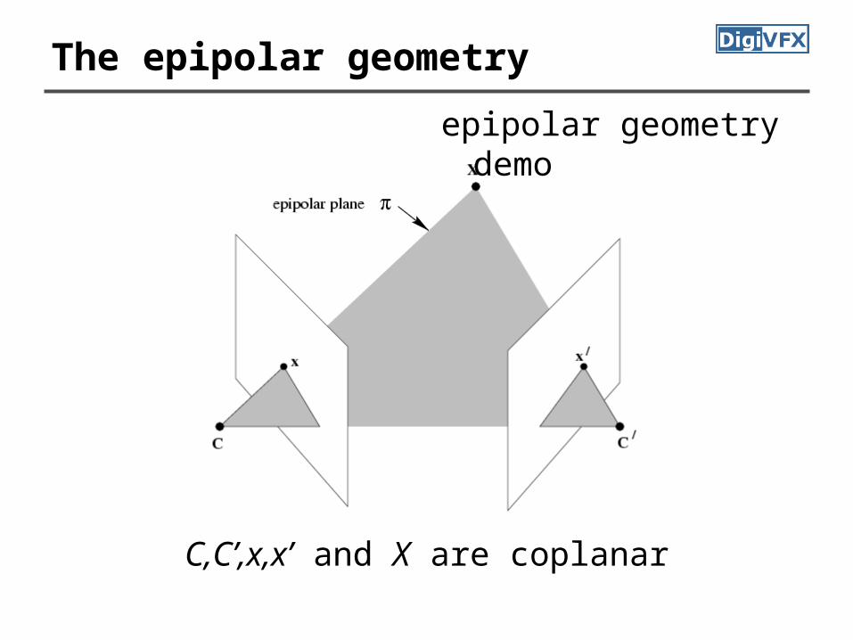
The epipolar geometry
C,C’,x,x’ and X are coplanar
epipolar geometry demo
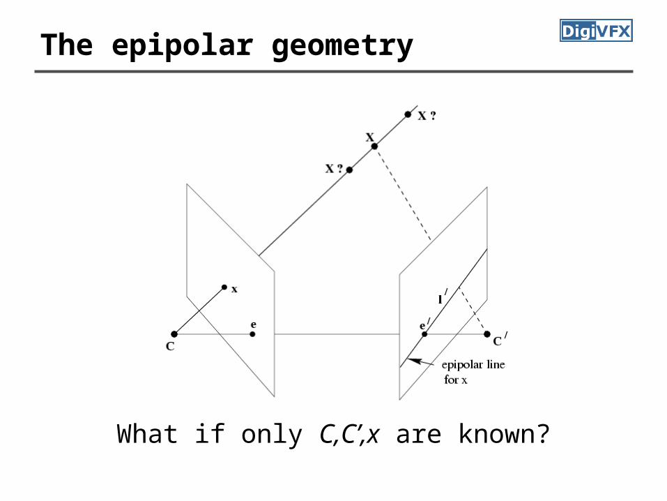
The epipolar geometry
What if only C,C’,x are known?
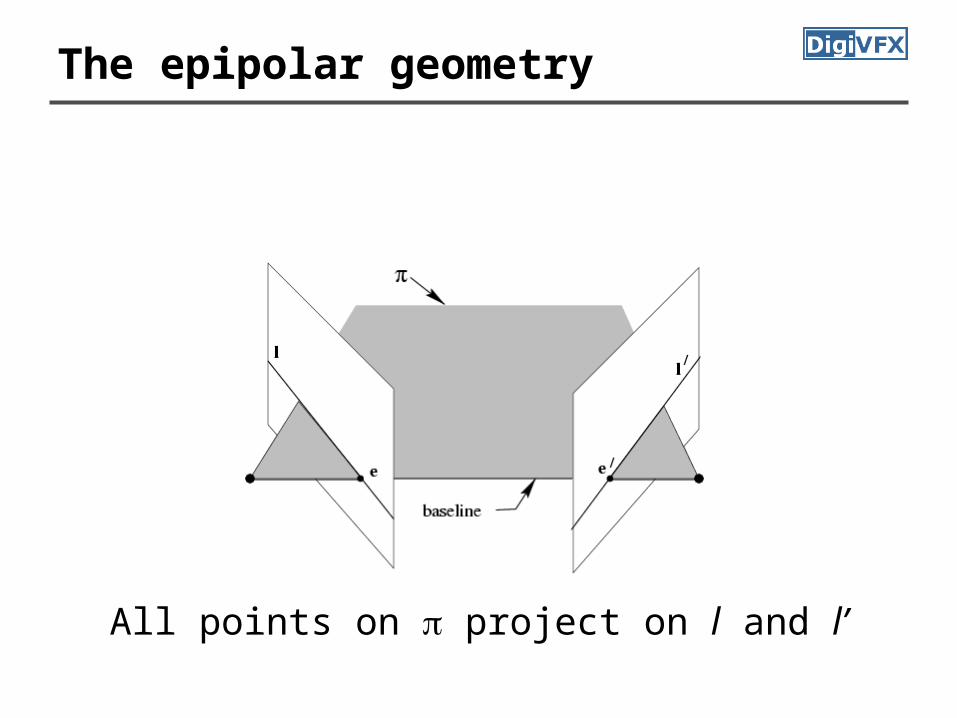
The epipolar geometry
All points on project on l and l’
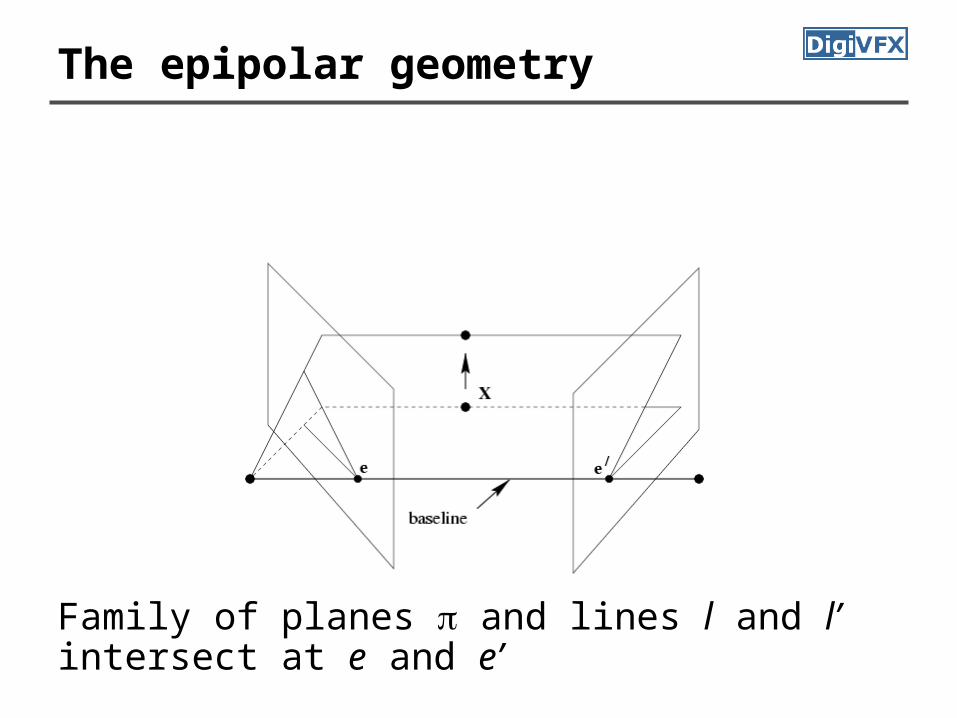
The epipolar geometry
Family of planes and lines l and l’ intersect at e and e’
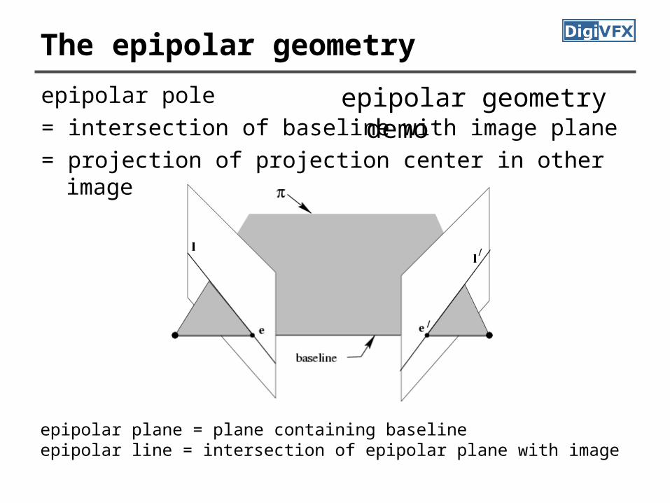
The epipolar geometry
epipolar plane = plane containing baselineepipolar line = intersection of epipolar plane with image
epipolar pole= intersection of baseline with image plane = projection of projection center in other image
epipolar geometry demo
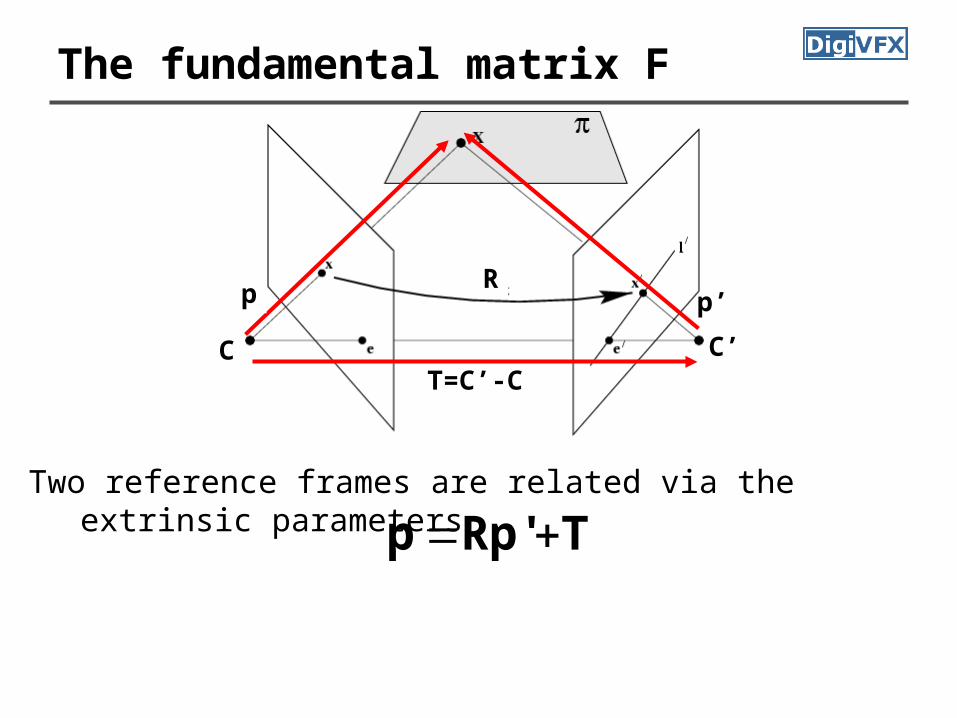
The fundamental matrix F
C C’T=C’-C
Rp p’
TRp'p Two reference frames are related via the extrinsic
parameters
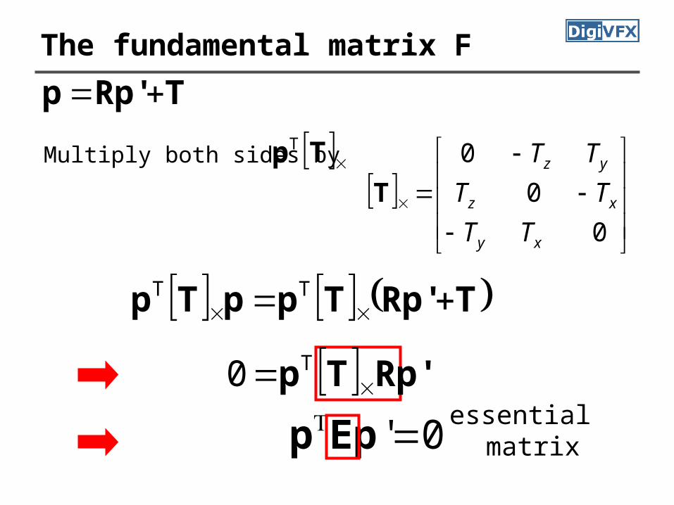
The fundamental matrix F
0'Eppessential
matrix
TRp'p
0
0
0
xy
xz
yz
TT
TT
TT
T
Multiply both sides by TpT
TRp'TppTp TT
Rp'Tp T0
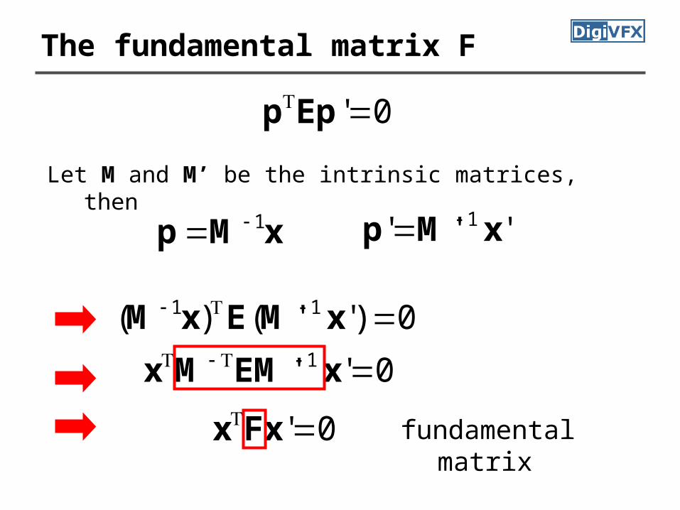
The fundamental matrix F
0'Epp
Let M and M’ be the intrinsic matrices, then
xMp 1 ''' 1 xMp
0)''()( 11 xMExM
0'' 1 xEMMx
0'Fxx fundamental matrix
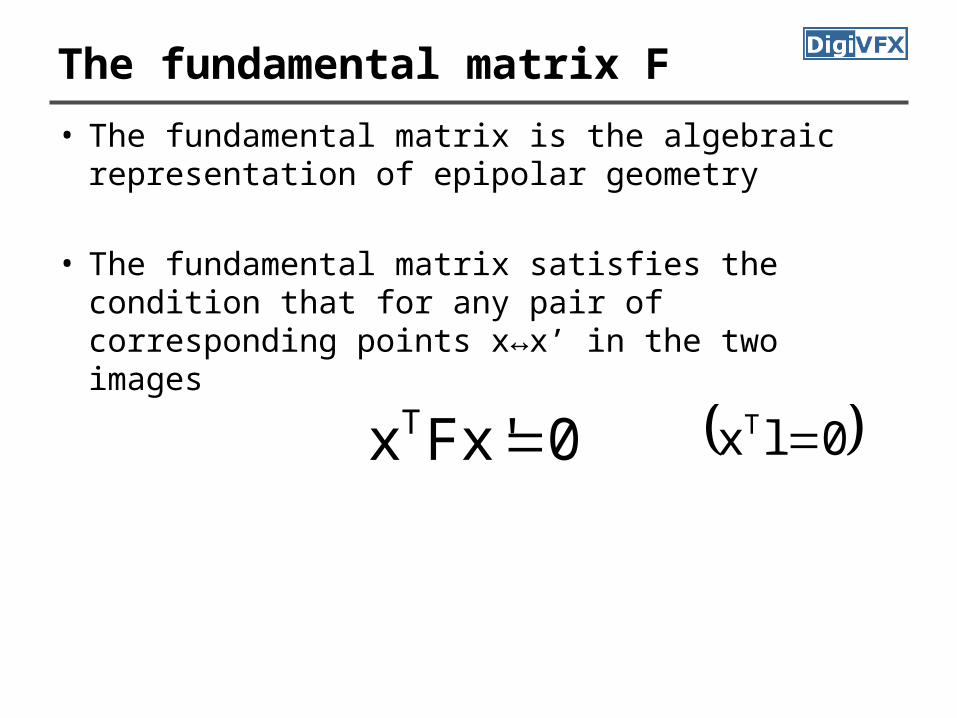
The fundamental matrix F
• The fundamental matrix is the algebraic representation of epipolar geometry
• The fundamental matrix satisfies the condition that for any pair of corresponding points x↔x’ in the two images
0Fx'xT 0lxT

F is the unique 3x3 rank 2 matrix that satisfies xTFx’=0 for all x↔x’
1. Transpose: if F is fundamental matrix for (P,P’), then FT is fundamental matrix for (P’,P)
2. Epipolar lines: l=Fx’ & l’=FTx3. Epipoles: on all epipolar lines, thus eTFx’=0, x’ eTF=0, similarly Fe’=0
4. F has 7 d.o.f. , i.e. 3x3-1(homogeneous)-1(rank2)5. F is a correlation, projective mapping from a point
x to a line l=Fx’ (not a proper correlation, i.e. not invertible)
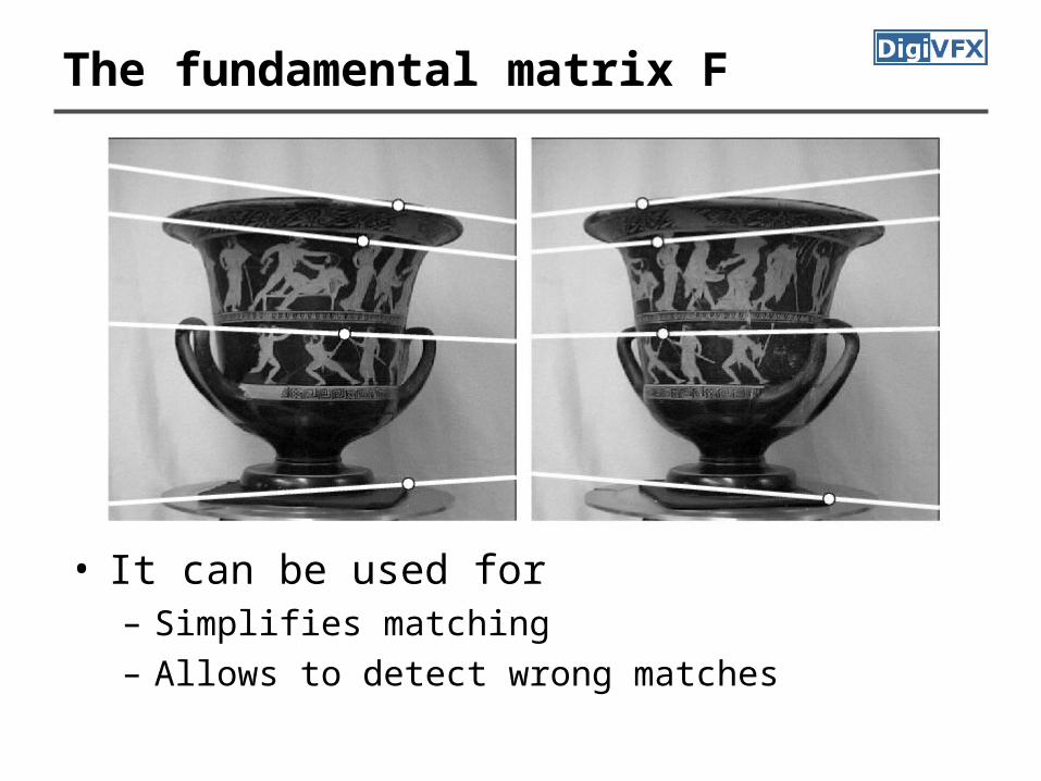
The fundamental matrix F
The fundamental matrix F
• It can be used for – Simplifies matching– Allows to detect wrong matches
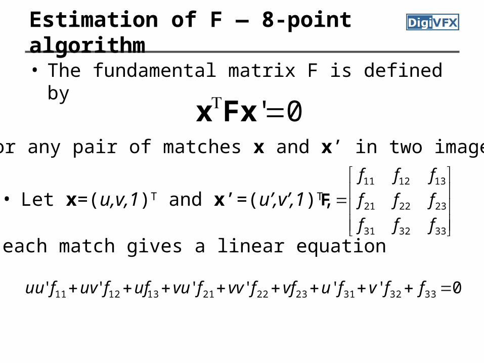
Estimation of F — 8-point algorithm• The fundamental matrix F is defined by
0'Fxxfor any pair of matches x and x’ in two images.
• Let x=(u,v,1)T and x’=(u’,v’,1)T,
333231
232221
131211
fff
fff
fff
F
each match gives a linear equation
0'''''' 333231232221131211 ffvfuvffvvfvuuffuvfuu

8-point algorithm
0
1´´´´´´
1´´´´´´
1´´´´´´
33
32
31
23
22
21
13
12
11
222222222222
111111111111
f
f
f
f
f
f
f
f
f
vuvvvuvuvuuu
vuvvvuvuvuuu
vuvvvuvuvuuu
nnnnnnnnnnnn
• In reality, instead of solving , we seek f to minimize subj. . Find the vector corresponding to the least singular value.
0AfAf 1f
8-point algorithm
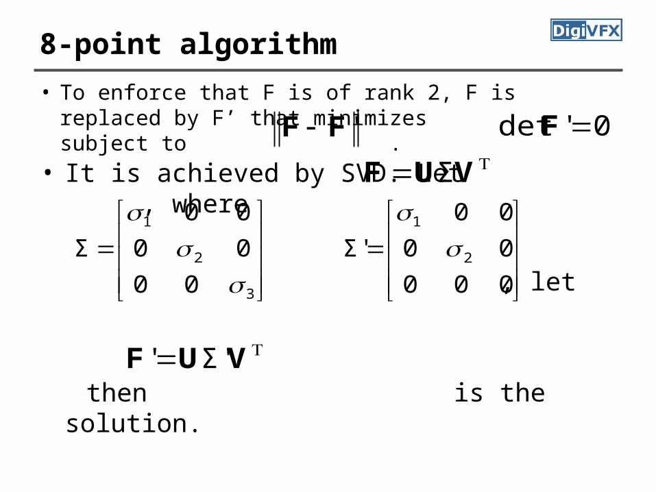
• To enforce that F is of rank 2, F is replaced by F’ that minimizes subject to . 'FF 0'det F
• It is achieved by SVD. Let , where
, let
then is the solution.
VUF Σ
3
2
1
00
00
00
Σ
000
00
00
Σ' 2
1
VUF Σ''
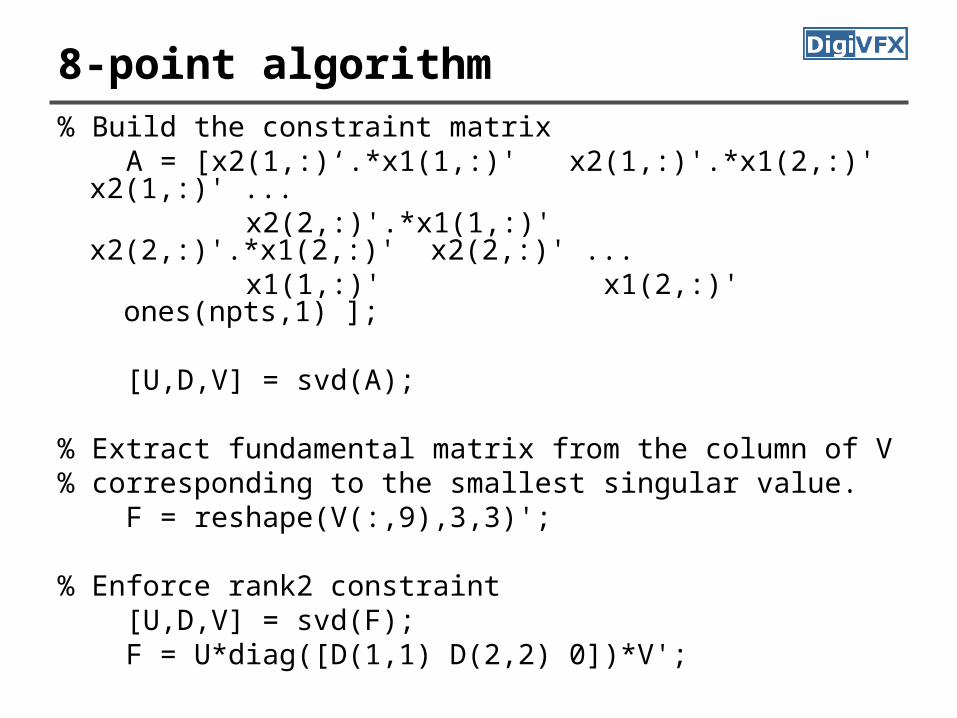
8-point algorithm% Build the constraint matrix A = [x2(1,:)‘.*x1(1,:)' x2(1,:)'.*x1(2,:)' x2(1,:)' ... x2(2,:)'.*x1(1,:)' x2(2,:)'.*x1(2,:)' x2(2,:)' ... x1(1,:)' x1(2,:)' ones(npts,1) ];
[U,D,V] = svd(A); % Extract fundamental matrix from the column of V % corresponding to the smallest singular value. F = reshape(V(:,9),3,3)'; % Enforce rank2 constraint [U,D,V] = svd(F); F = U*diag([D(1,1) D(2,2) 0])*V';

8-point algorithm
• Pros: it is linear, easy to implement and fast
• Cons: susceptible to noise
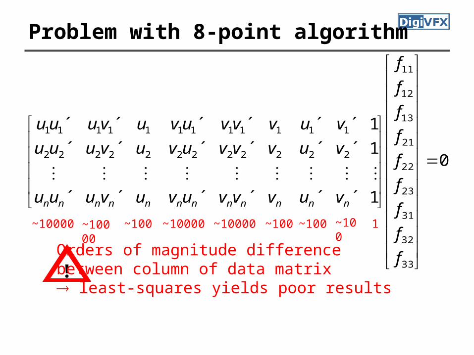
Problem with 8-point algorithm
~10000 ~10000 ~10000 ~10000~100 ~100 1~100 ~100
!Orders of magnitude differencebetween column of data matrix least-squares yields poor results
0
1´´´´´´
1´´´´´´
1´´´´´´
33
32
31
23
22
21
13
12
11
222222222222
111111111111
f
f
f
f
f
f
f
f
f
vuvvvuvuvuuu
vuvvvuvuvuuu
vuvvvuvuvuuu
nnnnnnnnnnnn

Normalized 8-point algorithm
1.Transform input by ,2.Call 8-point on to obtain3.
ii Txx ˆ 'i
'i Txx ˆ
'ii xx ˆ,ˆ
TFTF ˆΤ'F̂
0Fxx'
0ˆ'ˆ 1 xFTTx'
F̂
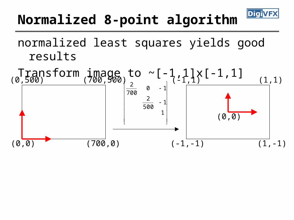
Normalized 8-point algorithm
(0,0)
(700,500)
(700,0)
(0,500)
(1,-1)
(0,0)
(1,1)(-1,1)
(-1,-1)
1
1500
2
10700
2
normalized least squares yields good resultsTransform image to ~[-1,1]x[-1,1]
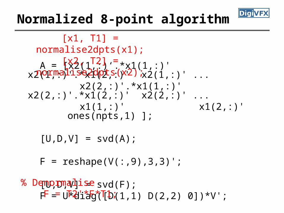
Normalized 8-point algorithm
A = [x2(1,:)‘.*x1(1,:)' x2(1,:)'.*x1(2,:)' x2(1,:)' ... x2(2,:)'.*x1(1,:)' x2(2,:)'.*x1(2,:)' x2(2,:)' ... x1(1,:)' x1(2,:)' ones(npts,1) ];
[U,D,V] = svd(A); F = reshape(V(:,9),3,3)'; [U,D,V] = svd(F); F = U*diag([D(1,1) D(2,2) 0])*V'; % Denormalise F = T2'*F*T1;
[x1, T1] = normalise2dpts(x1);
[x2, T2] = normalise2dpts(x2);
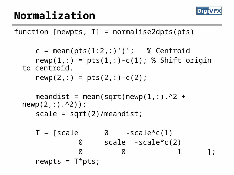
Normalization
function [newpts, T] = normalise2dpts(pts)
c = mean(pts(1:2,:)')'; % Centroid newp(1,:) = pts(1,:)-c(1); % Shift origin to centroid. newp(2,:) = pts(2,:)-c(2); meandist = mean(sqrt(newp(1,:).^2 +
newp(2,:).^2)); scale = sqrt(2)/meandist; T = [scale 0 -scale*c(1) 0 scale -scale*c(2) 0 0 1 ]; newpts = T*pts;
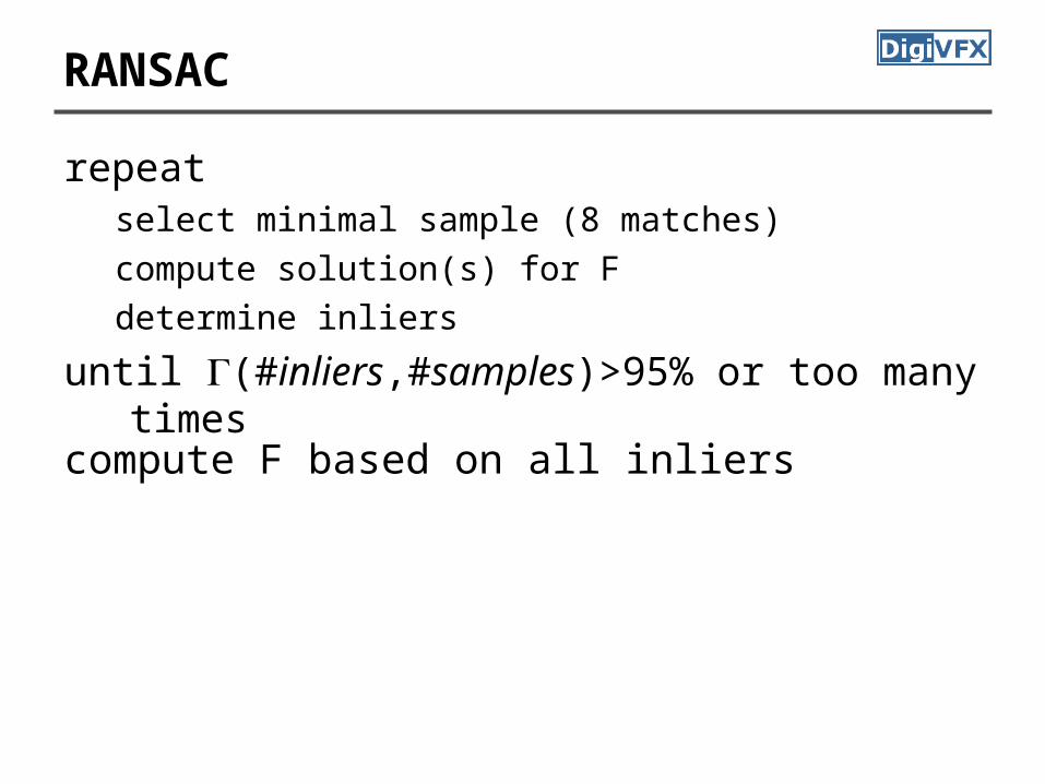
RANSAC
repeatselect minimal sample (8 matches)compute solution(s) for Fdetermine inliers
until (#inliers,#samples)>95% or too many times
compute F based on all inliers
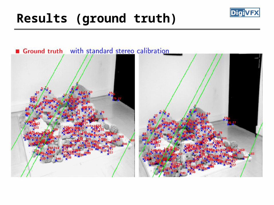
Results (ground truth)
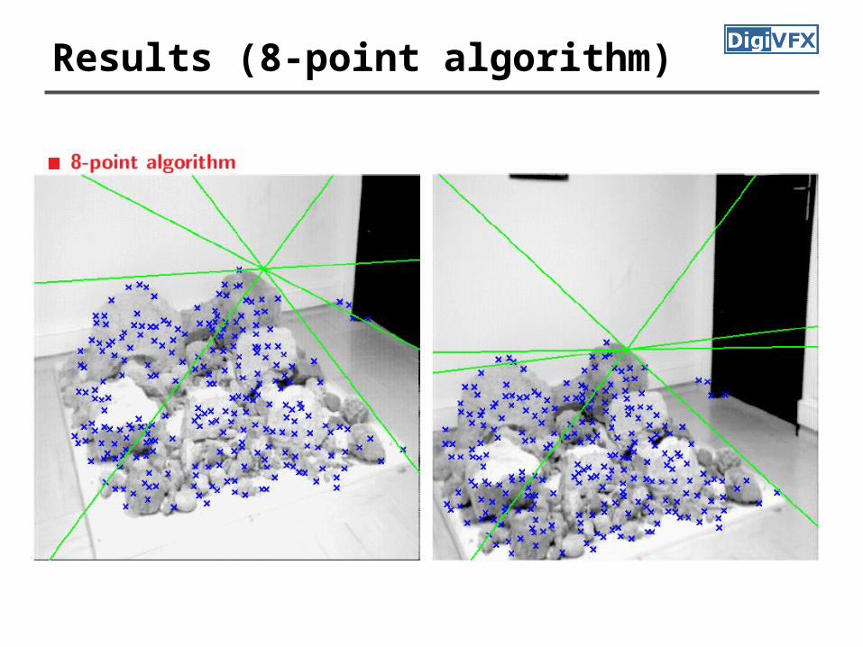
Results (8-point algorithm)
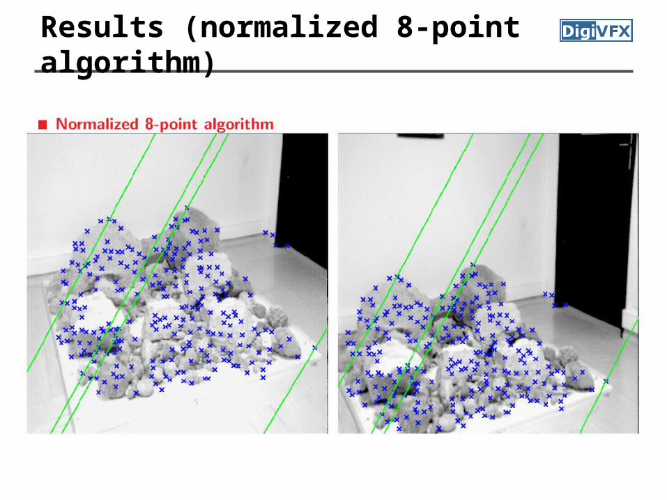
Results (normalized 8-point algorithm)

Structure from motion
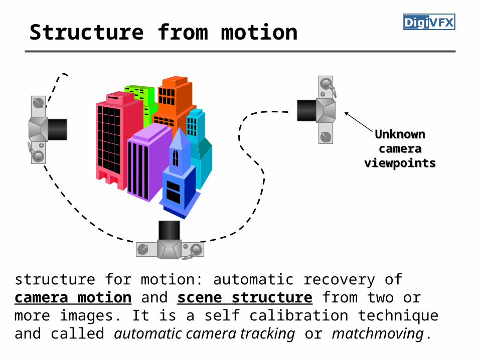
Structure from motion
structure for motion: automatic recovery of camera motion and scene structure from two or more images. It is a self calibration technique and called automatic camera tracking or matchmoving.
UnknownUnknowncameracamera
viewpointsviewpoints
Applications
• For computer vision, multiple-view shape reconstruction, novel view synthesis and autonomous vehicle navigation.
• For film production, seamless insertion of CGI into live-action backgrounds
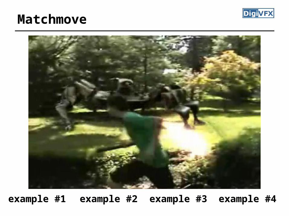
Matchmove
example #1 example #2 example #3 example #4
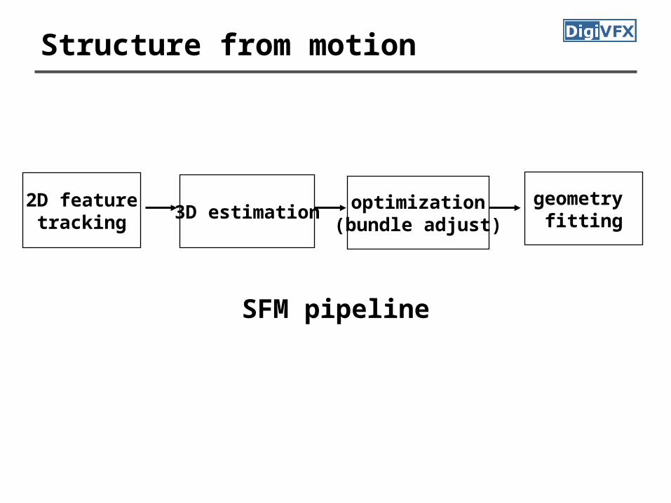
Structure from motion
2D featuretracking
3D estimation optimization(bundle adjust)
geometry fitting
SFM pipeline
Structure from motion
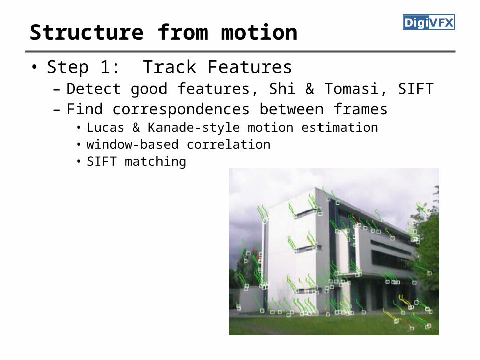
• Step 1: Track Features– Detect good features, Shi & Tomasi, SIFT– Find correspondences between frames
• Lucas & Kanade-style motion estimation• window-based correlation• SIFT matching

KLT tracking
http://www.ces.clemson.edu/~stb/klt/

Structure from Motion• Step 2: Estimate Motion and Structure
– Simplified projection model, e.g., [Tomasi 92]– 2 or 3 views at a time [Hartley 00]
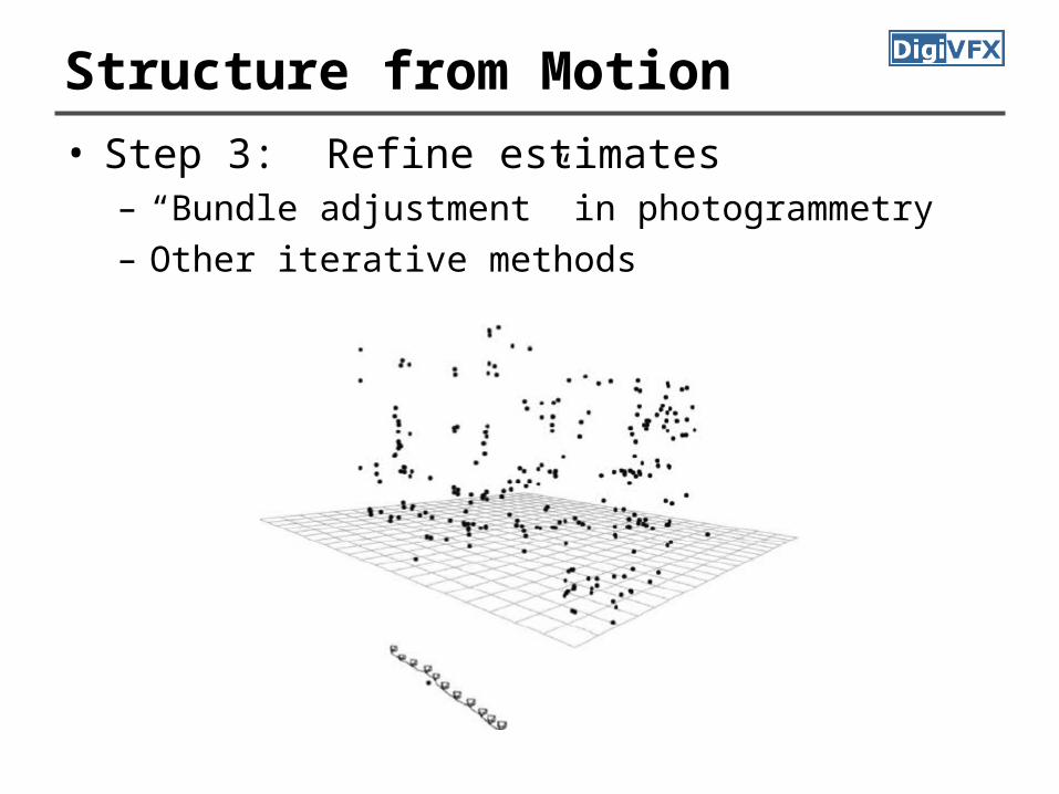
Structure from Motion• Step 3: Refine estimates
– “Bundle adjustment” in photogrammetry– Other iterative methods
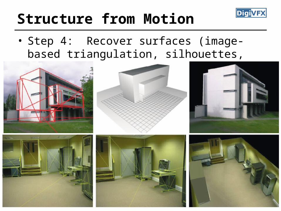
Structure from Motion• Step 4: Recover surfaces (image-based
triangulation, silhouettes, stereo…)
Good mesh

Factorization methods

Problem statement

Notations
• n 3D points are seen in m views• q=(u,v,1): 2D image point• p=(x,y,z,1): 3D scene point : projection matrix : projection function
• qij is the projection of the i-th point on image j
ij projective depth of qij)( ijij pq )/,/(),,( zyzxzyx zij

Structure from motion
• Estimate and to minimize
));((log),,,,,(1 1
11 ijij
m
j
n
iijnm Pw qpΠppΠΠ
otherwise
j in view visibleis if
0
1 iij
pw
• Assume isotropic Gaussian noise, it is reduced to
2
1 111 )(),,,,,( ijij
m
j
n
iijnm w qpΠppΠΠ
j ip
• Start from a simpler projection model
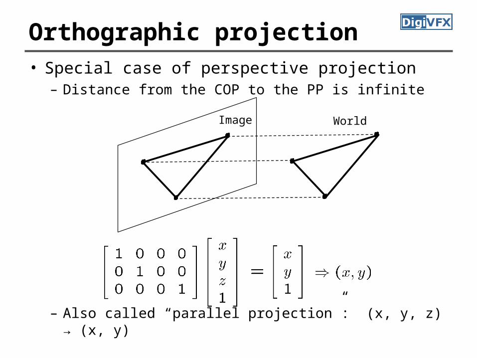
Orthographic projection• Special case of perspective projection
– Distance from the COP to the PP is infinite
– Also called “parallel projection”: (x, y, z) → (x, y)
Image World

SFM under orthographic projection
2D image point
Orthographic projectionincorporating 3D rotation3D scene
point
imageoffset
tΠpq 12 32 13 12
• Trick– Choose scene origin to be centroid of 3D points– Choose image origins to be centroid of 2D
points– Allows us to drop the camera translation:
Πpq
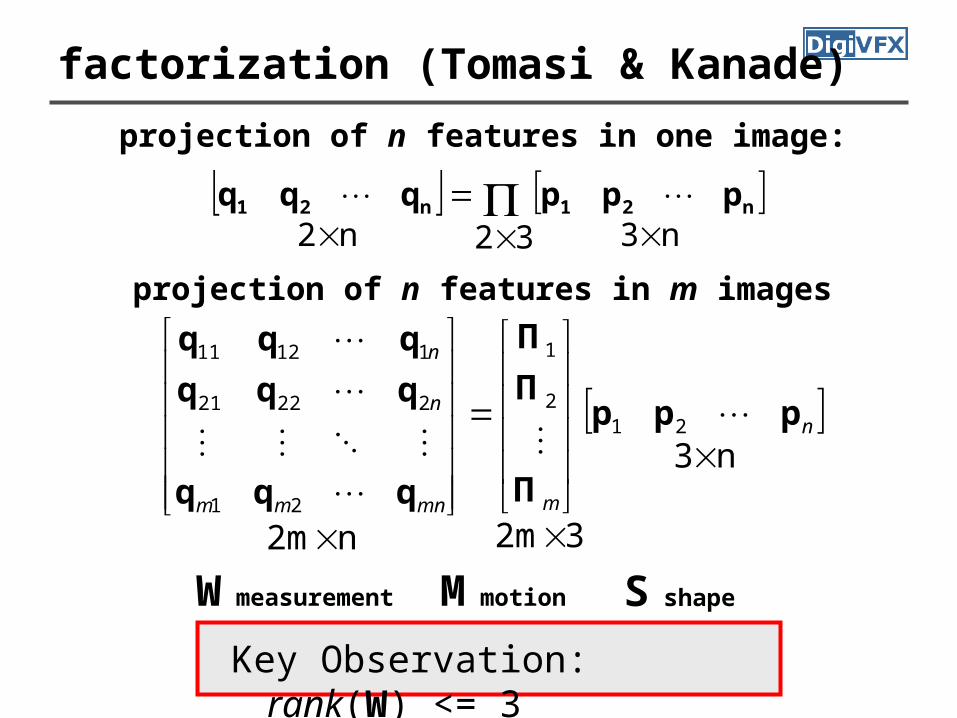
factorization (Tomasi & Kanade)
n332n2
n21n21 pppqqq
projection of n features in one image:
n3
32mn2m
212
1
21
22221
11211
n
mmnmm
n
n
ppp
Π
Π
Π
qqq
qqq
qqq
projection of n features in m images
W measurement M motion S shape
Key Observation: rank(W) <= 3
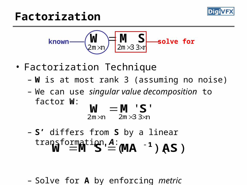
n33m2n2m''
SMW
• Factorization Technique– W is at most rank 3 (assuming no noise)– We can use singular value decomposition to
factor W:
Factorization
– S’ differs from S by a linear transformation A:
– Solve for A by enforcing metric constraints on M
))(('' ASMASMW 1
n33m2n2m SMWknown solve for
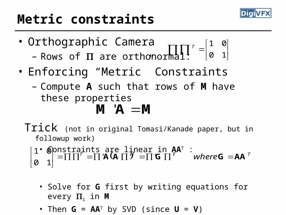
Metric constraints
• Orthographic Camera– Rows of are orthonormal:
• Enforcing “Metric” Constraints– Compute A such that rows of M have these
propertiesMAM '
10
01T
Trick (not in original Tomasi/Kanade paper, but in followup work)
• Constraints are linear in AAT :
• Solve for G first by writing equations for every i in M
• Then G = AAT by SVD (since U = V)
TTTT where AAGGAA
''''
10
01
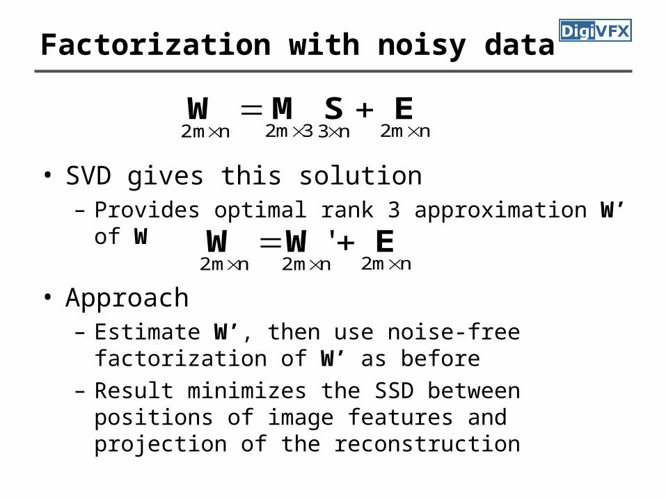
nm2n33m2n2m ESMW
Factorization with noisy data
• SVD gives this solution– Provides optimal rank 3 approximation W’ of W
nm2n2mn2m'
EWW
• Approach– Estimate W’, then use noise-free factorization
of W’ as before– Result minimizes the SSD between positions of
image features and projection of the reconstruction
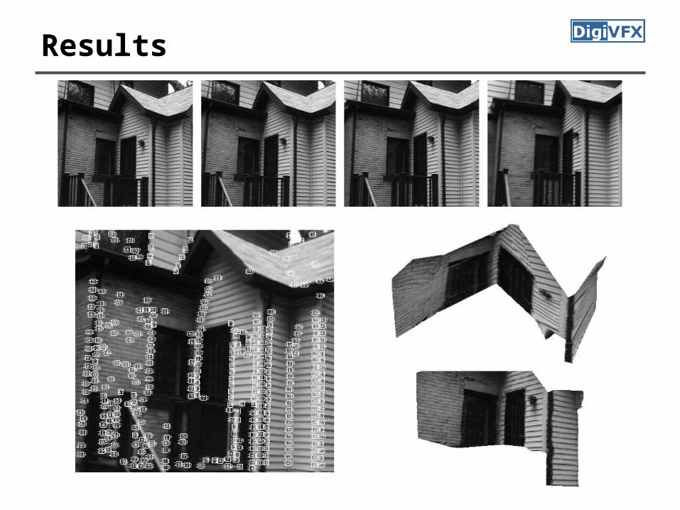
Results
Extensions to factorization methods• Projective projection• With missing data• Projective projection with missing data

Bundle adjustment
Levenberg-Marquardt method
• LM can be thought of as a combination of steepest descent and the Newton method. When the current solution is far from the correct one, the algorithm behaves like a steepest descent method: slow, but guaranteed to converge. When the current solution is close to the correct solution, it becomes a Newton’s method.
Nonlinear least square
).(ˆ with ,ˆ
Here, minimal. is distance squared
that theso vector parameter best the
find try to, tsmeasuremen ofset aGiven
pxxx
p
x
f
T
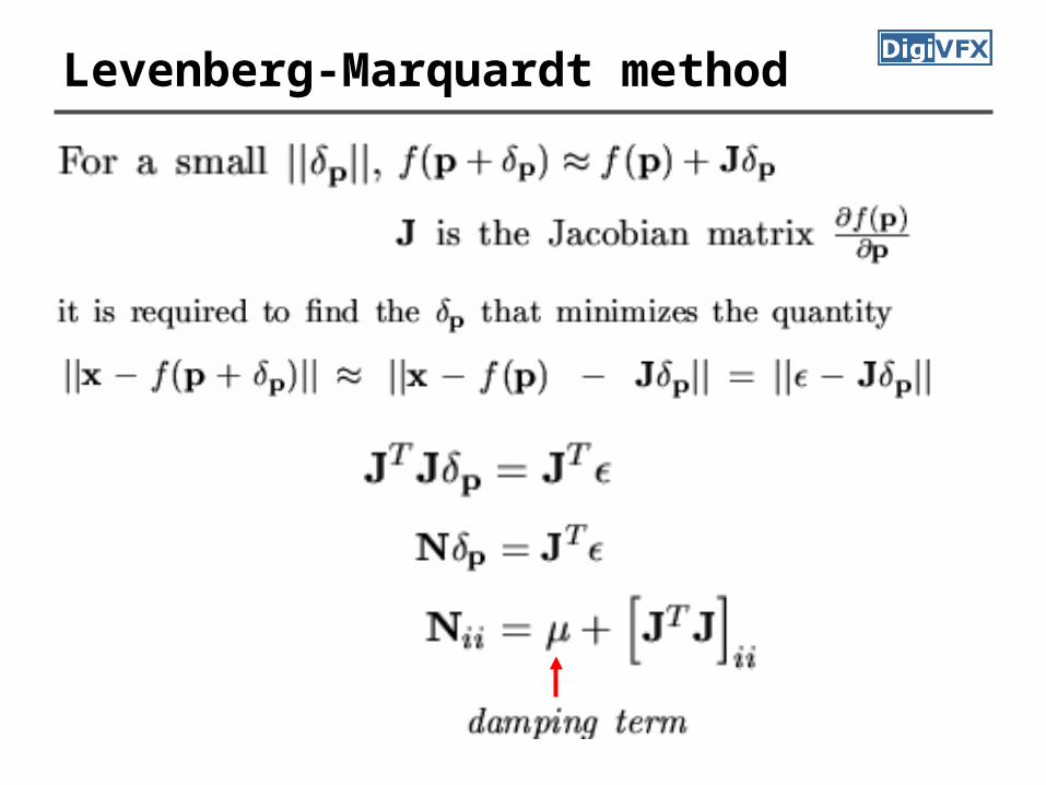
Levenberg-Marquardt method

Levenberg-Marquardt method
• μ=0 → Newton’s method• μ→∞ → steepest descent method
• Strategy for choosing μ– Start with some small μ– If error is not reduced, keep trying larger μ
until it does– If error is reduced, accept it and reduce μ for
the next iteration
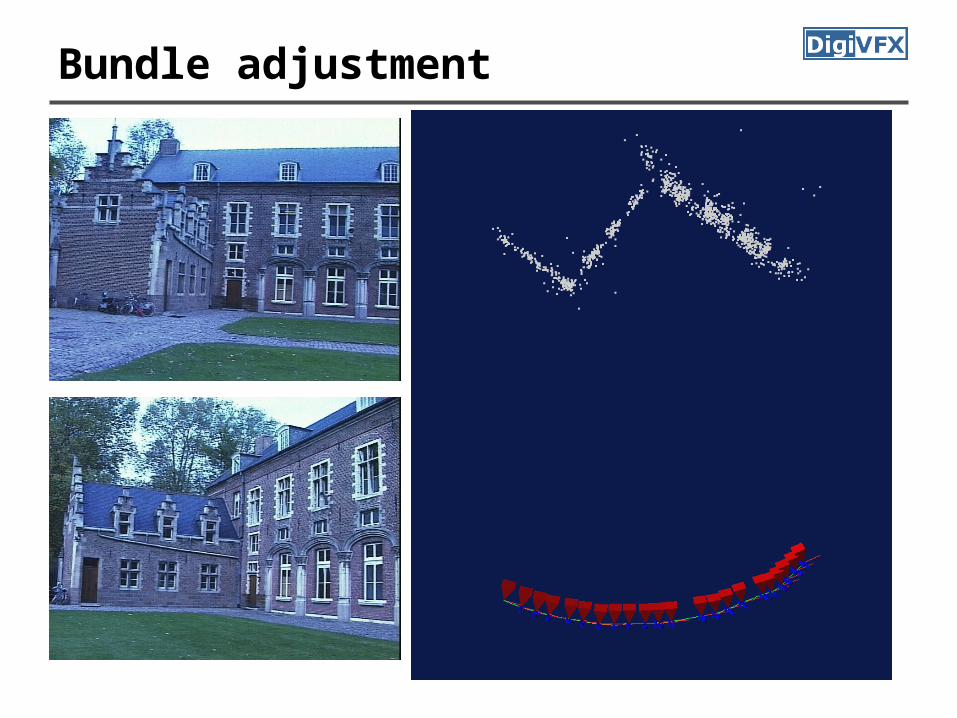
Bundle adjustment
• Bundle adjustment (BA) is a technique for simultaneously refining the 3D structure and camera parameters
• It is capable of obtaining an optimal reconstruction under certain assumptions on image error models. For zero-mean Gaussian image errors, BA is the maximum likelihood estimator.

Bundle adjustment
• n 3D points are seen in m views
• xij is the projection of the i-th point on image j
• aj is the parameters for the j-th camera
• bi is the parameters for the i-th point
• BA attempts to minimize the projection error
Euclidean distance
predicted projection
Bundle adjustment
Bundle adjustment
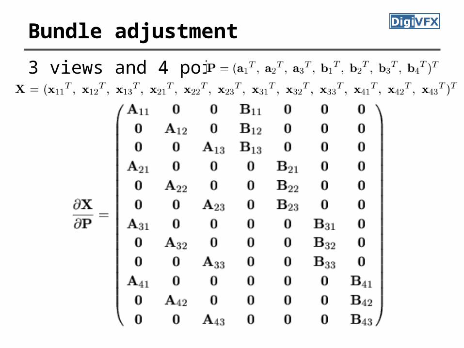
3 views and 4 points

Typical Jacobian
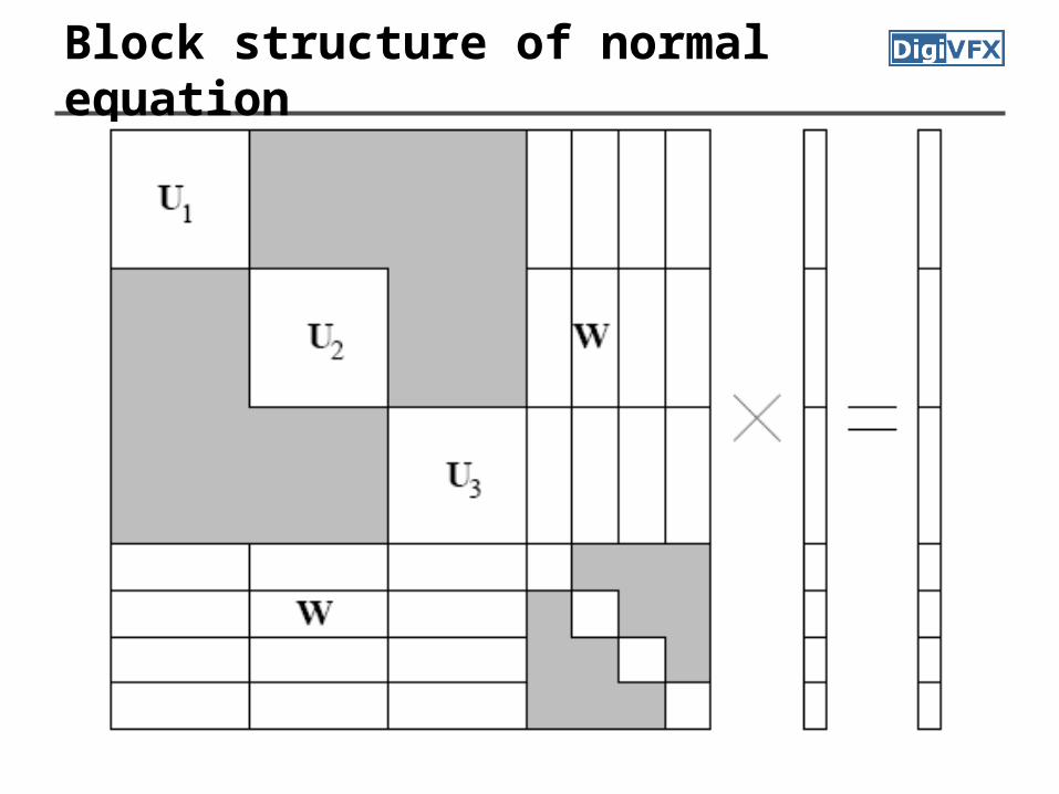
Block structure of normal equation

Bundle adjustment
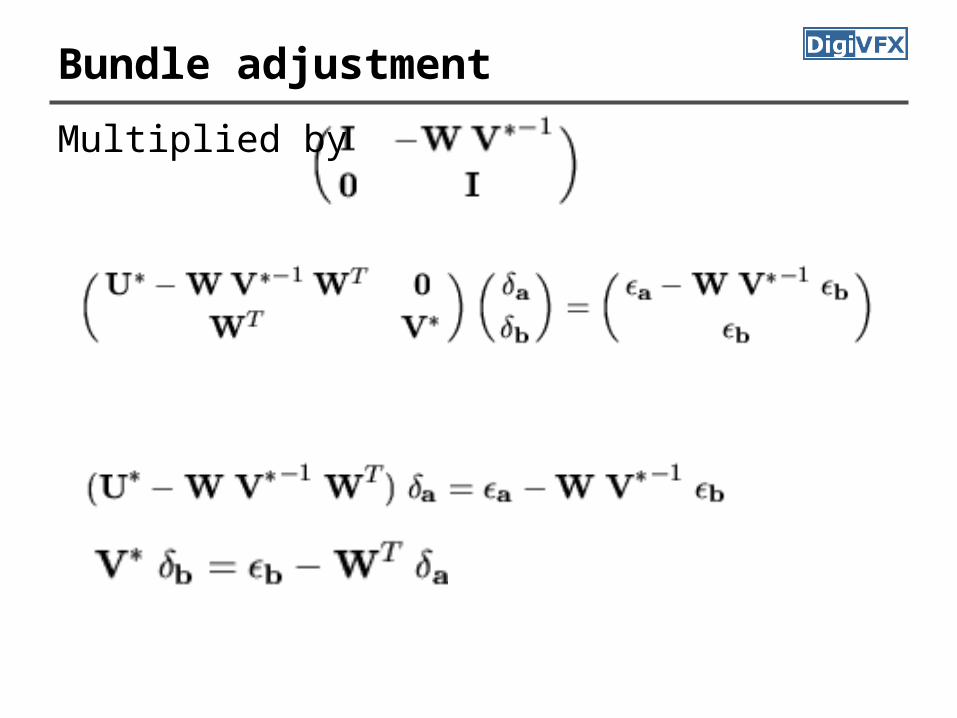
Bundle adjustment
Multiplied by
Issues in SFM
• Track lifetime• Nonlinear lens distortion• Degeneracy and critical surfaces• Prior knowledge and scene constraints• Multiple motions
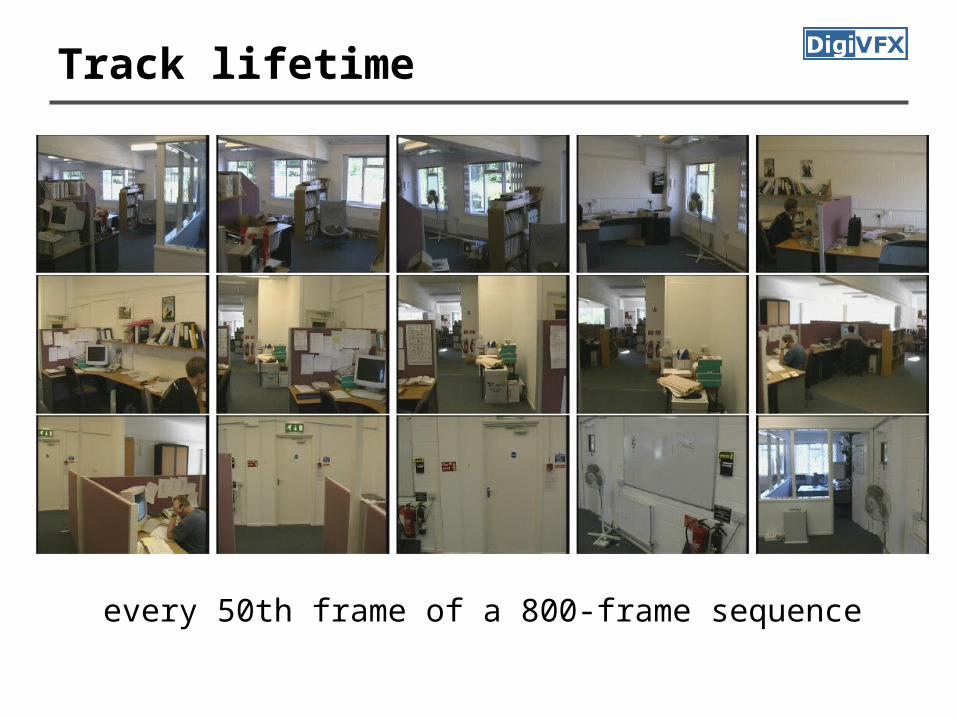
Track lifetime
every 50th frame of a 800-frame sequence
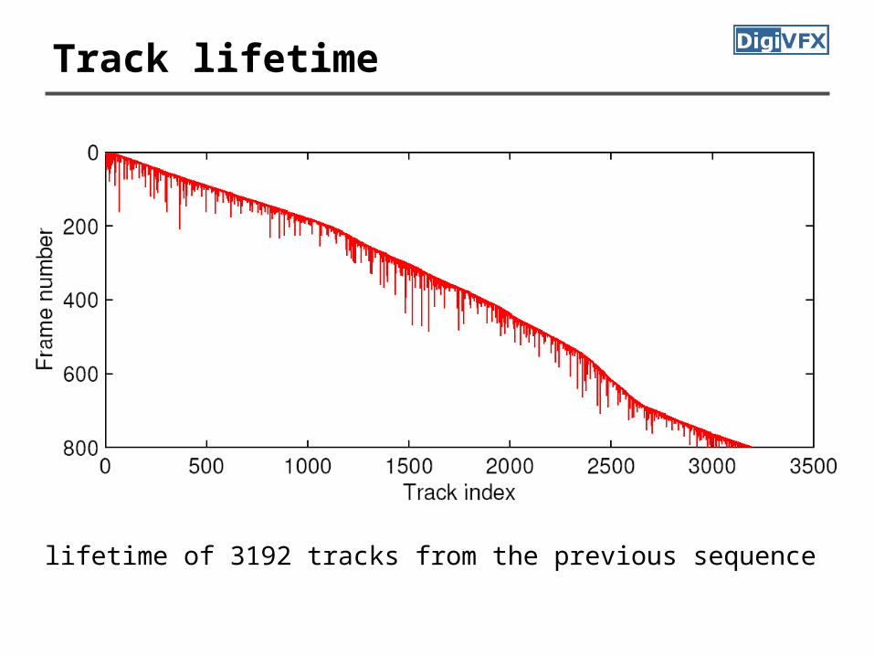
Track lifetime
lifetime of 3192 tracks from the previous sequence
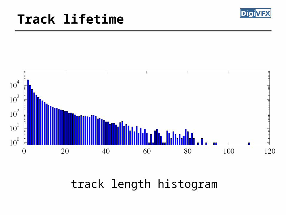
Track lifetime
track length histogram
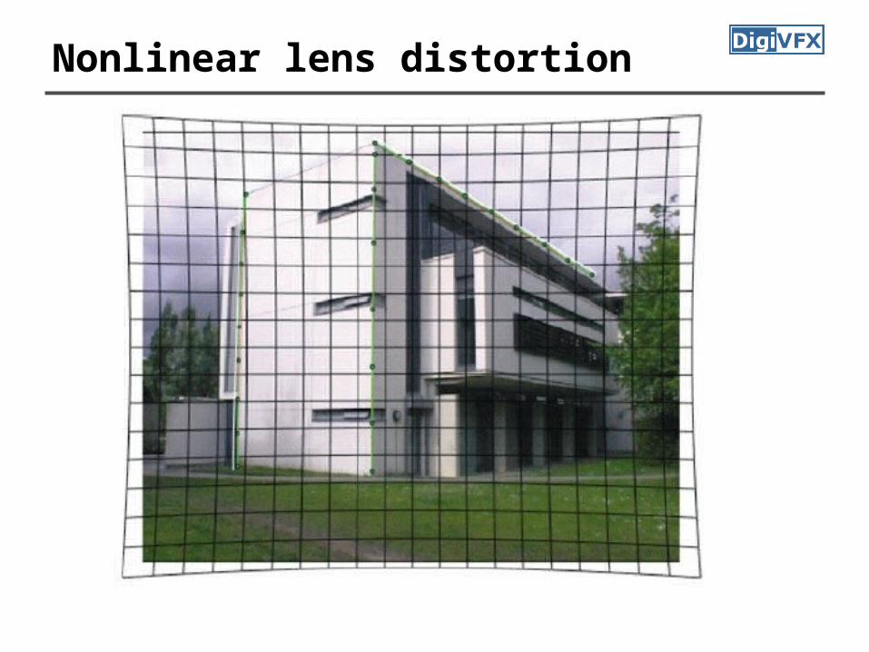
Nonlinear lens distortion
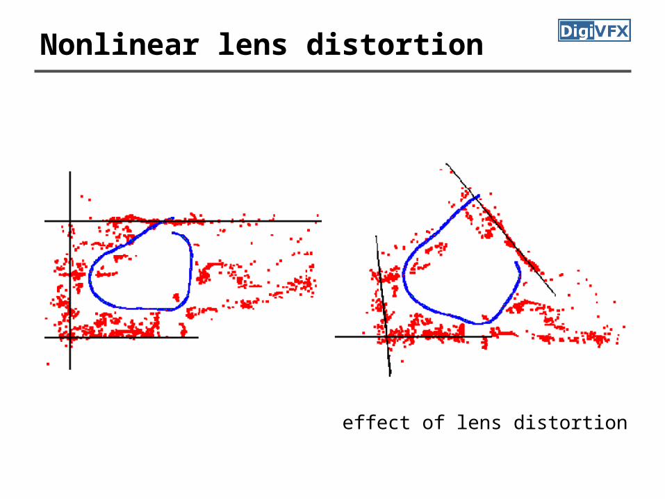
Nonlinear lens distortion
effect of lens distortion
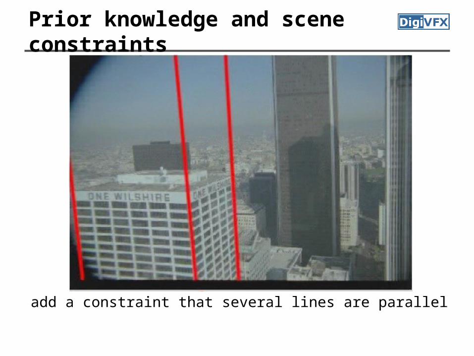
Prior knowledge and scene constraints
add a constraint that several lines are parallel
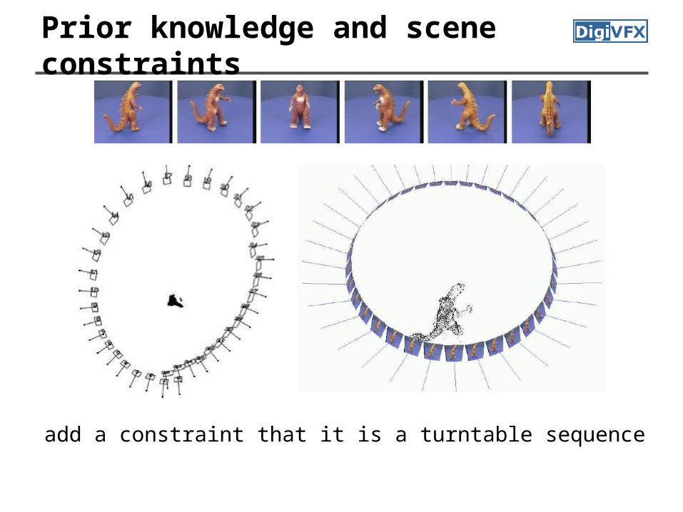
Prior knowledge and scene constraints
add a constraint that it is a turntable sequence

Applications of matchmove
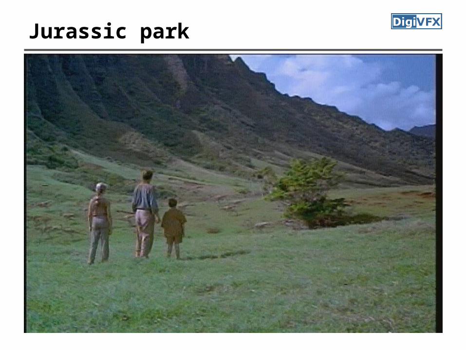
Jurassic park

2d3 boujou
Enemy at the Gate, Double Negative

2d3 boujou
Enemy at the Gate, Double Negative
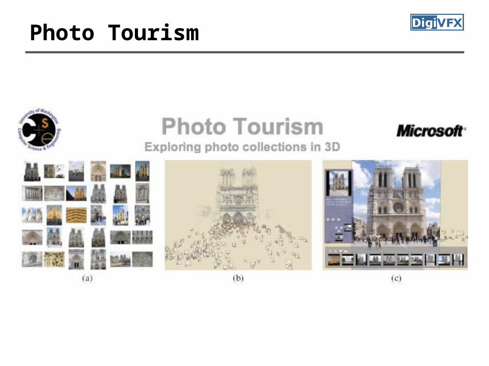
Photo Tourism
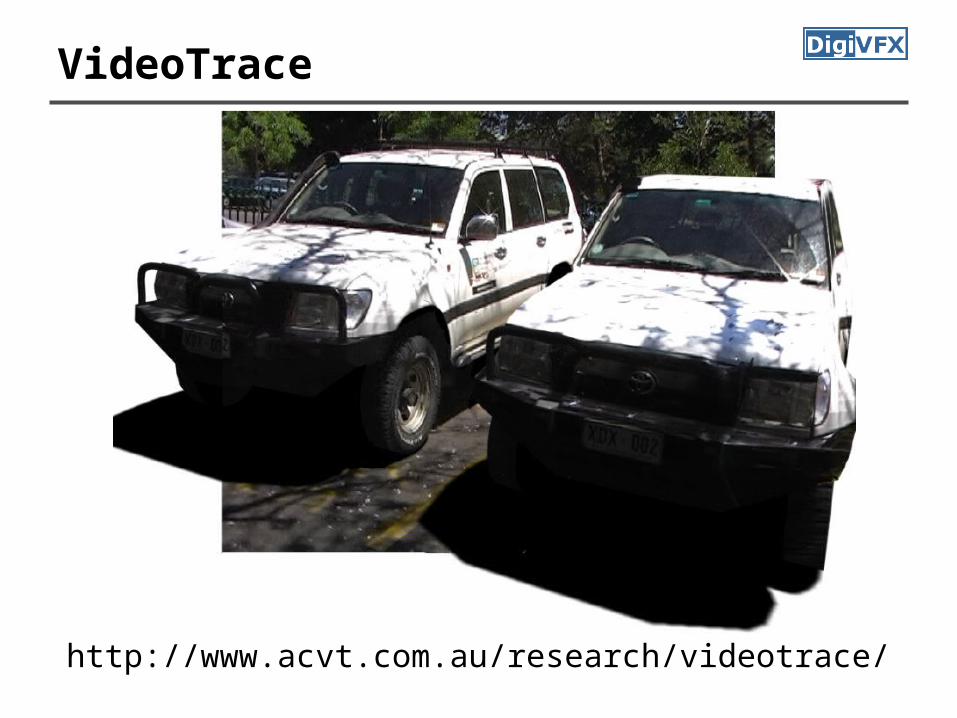
VideoTrace
http://www.acvt.com.au/research/videotrace/
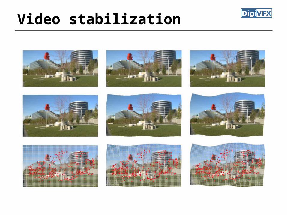
Video stabilization

Project #3 MatchMove
• It is more about using tools in this project• You can choose either calibration or
structure from motion to achieve the goal• Calibration • Voodoo/Icarus
• Examples from previous classes, #1, #2
References• Richard Hartley, In Defense of the 8-point Algorithm, ICCV,
1995. • Carlo Tomasi and Takeo Kanade, Shape and Motion from
Image Streams: A Factorization Method, Proceedings of Natl. Acad. Sci., 1993.
• Manolis Lourakis and Antonis Argyros, The Design and Implementation of a Generic Sparse Bundle Adjustment Software Package Based on the Levenberg-Marquardt Algorithm, FORTH-ICS/TR-320 2004.
• N. Snavely, S. Seitz, R. Szeliski, Photo Tourism: Exploring Photo Collections in 3D, SIGGRAPH 2006.
• A. Hengel et. al., VideoTrace: Rapid Interactive Scene Modelling from Video, SIGGRAPH 2007.