Structure determination of small and large molecules by ...

Structure determination of small and large

molecules using single crystal X-ray

crystallography

A thesis submitted to The University of Manchester for the degree

of Master of Science by Research in the Faculty of Engineering

and Physical Sciences

2010

Richard Prendergast

School of Chemistry

1

Structure determination of small and large molecules using single crystal X-ray crystallography

List of figures 4

List of tables 9

Abstract 10

Declaration 11

Copyright statement 12

Acknowledgements 13

Part A - Small molecule X-ray crystallography Chapter 1 - A review of the single crystal method Page 1.1 Basic Principles of X-ray crystallography 15

1.2 Diffraction of X-rays by crystals 16

1.3.1 Crystal structure and symmetry 17

1.3.2 The Bragg equation 22

1.3.3 Miller Indices 23

1.4.1 Nature, production and generation of X-rays 24

1.4.2 X-ray tube source 24

1.4.3 Synchrotron source 26

1.4.4 Detection of X-rays 27

1.5 Crystal growth 28

1.6.1 Structure determination procedure 30

1.6.2.1 The measurement of intensities 30

1.6.2.2 Preparation and mounting of the crystal 30

1.6.2.3 The collection of the X-ray intensities 32

1.6.2.4 The diffraction images data reduction process 32

1.6.3.1 The phase problem and possible solutions 33

1.6.3.2 The Patterson synthesis 34

1.6.3.3 Direct methods 35

1.6.4 Refining the structure 36

Chapter 2 - Structure determination of a small molecule – C26H36N8018Cl2Co

2

2.1 Introduction to C26H36N8018Cl2Co 38

2.2 X-ray diffraction data collection and processing procedure 38

2.3 Crystal structure analysis 40

2.4 Crystal structure implications 43

Chapter 3 - Structure determination of a small molecule – C26H36N8010F12P2Co 3.1 Introduction to C26H36N8010F12P2Co 44

3.2 X-ray diffraction data collection and processing procedure 44

3.3 Crystal structure analysis 46

3.4 Crystal structure implications 48

3.5 Comparison of the crystal structures 48

Chapter 4 - Structure determination of two small molecules – C30H24N04Sn & C30H20Sn 4.1 Introduction to C30H24N04Sn & C30H20Sn 52

4.2 X-ray diffraction data collection and processing procedure for C30H20Sn 53

4.3 X-ray diffraction data collection and processing procedure for C30H24N04Sn 55

4.4 Crystal structure analysis for C30H20Sn 56

4.5 Crystal structure analysis for C30H24N04Sn 59

4.6 Crystal structure implications of C30H20Sn 63

4.7 Crystal structure implications of C30H24N04Sn 64

Part B - Macromolecular X-ray crystallography Chapter 5 - Macromolecular X-ray crystallography 5.1 Introduction 67

5.2.1 Crystallisation techniques 68

5.2.2 The batch method 69

5.2.3 Dialysis 69

5.2.4 Vapour diffusion methods 69

5.2.5 Hot box technique 70

5.3.1 Solving the phase problem in macromolecular X-ray crystallography 70

5.3.2 Isomorphous replacement 70

5.3.3 Anomalous scattering 74

3

5.3.4 Molecular replacement 76

5.4 Rigid body and restrained refinement 77

5.5 The R free factor

78

Chapter 6 - Crystal structure determination and model refinement of a co-crystallisation of HEWL and TA6Br12

6.1 Introduction 79

6.1.2 Introduction to lysozyme 79

6.1.3 Introduction to Ta6Br12 80

6.2 Co-crystallisation procedure of HEWL and Ta6Br12 81

6.3 X-ray diffraction data collection procedure 82

6.4 The model refinement procedure 84

6.5 Refinement of the occupancies of the Ta6Br12 binding sites using SHELX 88

6.6 Analysis of the three dimensional structure 91

6.7 Implications of the three dimensional structure 98

Chapter 7 - Crystal structure determination and model refinement of a co-crystallisation of HEWL and Carboplatin 7.1.1 Introduction to carboplatin 99

7.1.2 Previous work by Casini et al 101

7.1.3 Previous work by the Helliwell group 101

7.2 Co-crystallisation procedure and optimisation of the conditions 102

7.3 X-ray diffraction data collection procedure 106

7.4 The model refinement procedure 108

7.5.1 Analysis of the three dimensional structure 111

7.5.2 Comparison with HEWL and cisplatin crystal structure 114

7.5.3 Comparison with previous HEWL and carboplatin crystal structure 116

7.5.4 Comparison with HEWL and NAG trisaccaride crystal structure 116

7.6 Implications of the three dimensional structure 117

Chapter 8 - Conclusions and future work 120 References 121 Bibliography 126

Word count = 26,292

4

List of figures

Chapter 1 Page

1.1 An example of a diffraction pattern. 16

1.2 An example of the lattice of a crystal. 18

1.3 An example of a unit cell with the constituent axes and angles

labelled. 18

1.4 The fourteen Bravais lattices. 20

1.5 A 21 screw axis. 22

1.6 A pictorial representation of the Bragg equation. 23

1.7 The 111 Miller plane. 24

1.8 The 010 Miller plane. 24

1.9 A schematic representation of an X-ray tube. 26

1.10 The vapour diffusion method for small molecule crystallisation. 29

1.11 The vapour diffusion method for macromolecular crystallisation. 30

1.12 A crystal mounted within a loop. 32

Chapter 2 Page

2.1 An ORTEP diagram of C26H36N8018Cl2Co with 50% ellipsoid

probability. 41

2.2 Figure to show hydrogen bonding arrangement between cobalt

malonate molecules to form one dimensional chains. 42

2.3 A figure to show the crystal packing arrangement of

C26H36N8018Cl2Co. 43

5

Chapter 3 Page

3.1 An ORTEP diagram of C26H36N8O10F12P2Co with 50% ellipsoid

probability. 46

3.2 A figure to show the crystal packing arrangement of

C26H36N8O10F12P2Co. 47

3.3 A figure illustrating the common hydrogen bonding motif which is

present in both structures C26H36N8O18Cl2Co and

C26H36N8O10F12P2Co.

49

3.4 A figure to illustrate the difference in the hydrogen bonding

arrangements around the PF6 and perchlorate counter ions. 50

Chapter 4 Page

4.1 The expected chemical structure of the molecule in the crystal

MHB7. 52

4.2 The expected chemical structure of the molecule in the crystal

MHB8. 52

4.3 An ORTEP diagram of C24H20Sn with 50% ellipsoid probability 57

4.4 A figure to show the location of eight weak H…C-H interactions that

each C24H20Sn molecule forms. 58

4.5 A figure to show the stacking of the C24H20Sn molecule within the

crystal.. 58

4.6 A figure to show the stacking of layers of C24H20Sn molecules

stabilised by weak van der Waals interactions. 59

4.7 An ORTEP diagram of C30H24NO4Sn with 50% ellipsoid probability. 60

4.8 A figure to show the arrangement of the polymeric chains in

C30H24NO4Sn with weak van der Waals interactions shown as blue 61

6

lines. Hydrogen atoms are omitted for clarity.

4.9 A figure to show the distance between aromatic phenyl rings in

C30H24NO4Sn. Hydrogen atoms are omitted for clarity. 61

4.10 A figure to show the intramolecular hydrogen bond present within

the monomeric units. 62

4.11 A figure to show how SHELX views the molecules as discrete units

and not as a polymeric structure. 63

4.12 The crystallographically determined structure has this chemical

diagram with the highlighted area corresponding to the deviation

from the expected chemical structure.

65

Chapter 5 Page

5.1 The crystal growth phases. 68

5.2 A vectorial representation of the isomorphous replacement method. 72

5.3 A Harker construction for a native protein and a single heavy atom

derivative. 73

5.4 A Harker construction for a native protein and a second heavy atom

derivative. 74

Chapter 6 Page

6.1 The structure of the Ta6Br12 cluster. 80

6.2 A picture of the Ta6Br12 and HEWL crystals. 82

6.3 An X-ray diffraction pattern image from the Ta6Br12 & HEWL data

collection. 83

6.4 A figure to illustrate the gradual reduction of the conventional R

factor with each step of refinement performed.

88

7

6.5 A figure to show the evolution of the occupancies of the four binding

sites versus each step of refinement 91

6.6 A figure showing the electron density around the first Ta6Br12 to

lysozyme binding site. 92

6.7 A figure to show the distances between the tantalum atoms in the first

Ta6Br12 to lysozyme binding site. 92

6.8 A figure showing the electron density around the second Ta6Br12 to


6.9 A figure to show the distances between the tantalum atoms in the

second Ta6Br12 to lysozyme binding site. 94

6.10 A figure showing the electron density around the third Ta6Br12 to



third Ta6Br12 to lysozyme binding site. 96

6.12 A figure showing the electron density around the fourth Ta6Br12 to



fourth Ta6Br12 to lysozyme binding site. 98

Chapter 7 Page

7.1 The chemical structure of cisplatin. 99

7.2 The chemical structure of carboplatin. 99

7.3 A picture of the carboplatin and HEWL crystals. 105

7.4 A picture of an aggregate of carboplatin and HEWL crystals. 106

7.5 A picture of a carboplatin and HEWL crystal mounted onto a loop. 106

7.6 An X-ray diffraction pattern image from the carboplatin and HEWL

data collection. 108

8

7.7 A figure to illustrate the gradual reduction of the conventional R

factor with each step of refinement performed. 111

7.8 A figure to show the distances from the platinum atom to the two

ammonia groups in both carboplatin to lysozyme binding sites. 112

7.9 A figure to show the distances from the platinum atom to the nearest

nitrogen atom on the histidine 15 residue for both binding sites 113

7.10 A figure to show the electron density around the binding site present

on the left hand side of histidine 15. 113

7.11 A figure to show the electron density around the binding site present

on the right hand side of histidine 15. 114

7.12 A figure showing the superimposition of the histidine 15 residue in a

crystal of cisplatin and HEWL and a crystal of carboplatin and

HEWL.

115

7.13 A figure displaying the location of the DMSO molecule present

within the lysozyme active site for both the cisplatin and carboplatin

models.

116

7.14 Figure 7.13 – A figure showing the location of a NAG trisaccharide

and the DMSO molecules present in the cisplatin and carboplatin

models.

117

9

List of tables

Table Page

1 The essential symmetry and unit cell restrictions of the seven crystal

systems. 19

2 A summary of the X-ray diffraction and crystal data for

C26H36N8018Cl2Co. 40

3 The hydrogen bonding details for structure C26H36N8O18Cl2Co. 41


C26H36N8O10F12P2Co. 45

5 The hydrogen bonding details for structure C26H36N8O10F12P2Co. 46

6 A summary of the X-ray diffraction and crystal data for C24H20Sn. 53


C30H24NO4Sn. 55

8 A comparison of the details of the original 1970 C24H20Sn structure

and the structure reported in this thesis. 64

9 A summary of the X-ray diffraction data collection of a Ta6Br12 and

HEWL crystal. 84

10 A summary of the conditions attempted in the crystallisation of

HEWL in the presence of DMSO. 103

11 A summary of the X-ray diffraction data collection of a carboplatin

and HEWL crystal. 107

10

The University of Manchester

Richard Prendergast

Msc. in Chemistry by Research - Structure determination of small and large

molecules using single crystal X-ray crystallography

06/09/2010

Abstract

Single crystal X-ray crystallography can be applied to the entire spectrum of molecular size. If performed correctly the result is an unambiguous, three dimensional image of all the atoms located within a molecule. This applies to small chemical structures all the way through to biological macromolecules. In this thesis the method is used to solve the crystal structures of four small molecules and in addition to two macromolecular adducts. The first two molecules studied were believed to be closely isomorphous cobalt containing structures. The first small molecule was found to be C26H36N8018Cl2Co and crystallised in the triclinic space group P 1 . The structure was solved with an R factor of 0.0309. The second small molecule was found to be C26H36N8O10F12P2Co and crystallised in the triclinic space group P 1 . The structure was solved with an R factor of 0.0313. The remaining two small molecules were believed to be closely isomorphous tin containing structures. The third small molecule was found to be Ph4Sn and crystallised in the tetragonal space group P 4 21/c. The structure was solved with an R factor of 0.0353. The fourth small molecule was found to be C30H24NO4Sn and crystallised in the triclinic space group P 1 . The structure was solved with an R factor of 0.0245. In addition the crystal packing of all four small molecules were analysed. The implications of the determined crystal structures are discussed in terms of the relevant literature in each case. The method was also used to determine the structure of two macromolecular adducts. The first was a co-crystallisation of hen egg white lysozyme and Ta6Br12. The model refinement and a description of the Ta6Br12 binding sites are included. The second was a co-crystallisation of hen egg white lysozyme and carboplatin with the solubility of the carboplatin optimised using DMSO, whilst still obtaining crystals. The model refinement and a description of the carboplatin binding sites are included. Finally conclusions and possible routes for future work are offered.

11

Declaration

I declare that no portion of the work referred to in this thesis has been submitted in

support of an application for another degree or qualification at this or any other university

or other institute of learning.

12

Copyright

i. The author of this thesis (including any appendices and/or schedules to this

thesis) owns certain copyright or related rights in it (the “Copyright”) and s/he

has given The University of Manchester certain rights to use such Copyright,

including for administrative purposes.

ii. Copies of this thesis, either in full or in extracts and whether in hard or

electronic copy, may be made only in accordance with the Copyright, Designs

and Patents Act 1988 (as amended) and regulations issued under it or, where

appropriate, in accordance with licensing agreements which the University has

from time to time. This page must form part of any such copies made.

iii. The ownership of certain Copyright, patents, designs, trade marks and other

intellectual property (the “Intellectual Property”) and any reproductions of

copyright works in the thesis, for example graphs and tables

(“Reproductions”), which may be described in this thesis, may not be owned

by the author and may be owned by third parties. Such Intellectual Property

and Reproductions cannot and must not be made available for use without the

prior written permission of the owner(s) of the relevant Intellectual Property

and/or Reproductions.

iv. Further information on the conditions under which disclosure, publication and

commercialisation of this thesis, the Copyright and any Intellectual Property

and/or Reproductions described in it may take place is available in the

University IP Policy (see

http://www.campus.manchester.ac.uk/medialibrary/policies/intellectual-

property.pdf), in any relevant Thesis restriction declarations deposited in the

University Library, The University Library’s regulations (see

http://www.manchester.ac.uk/library/aboutus/regulations

)

13

Acknowledgements

I would like to begin by thanking Professor John R. Helliwell for his supervision and

for allowing me this opportunity.

I am extremely grateful to Dr Madeline Helliwell and Dr George Habash for their

help and patience regarding small molecule and protein X-ray crystallography

respectively.

I would also like to thank Dr Jim Raftery for his advice and for stimulating

discussions regarding subjects ranging from crystallography to politics.

Finally, I would like to thank my parents. Their loving support has made this possible.

RJP

Manchester

2010

14

Part A – Small molecule X-ray crystallography

15

Chapter 1

A review of the single crystal method 1.1 – Basic principles of X-ray crystallography A simple analogy to help visualise the basic principles that underpin X-ray

crystallography is that of a simple optical microscope. In both microscopy and

crystallography it is useful to view radiation in terms of a travelling wave of energy as

opposed to a particle.

In the case of the optical microscope a light source provides visible light waves which

pass through the sample under study and are subsequently diffracted. Each of these

diffracted waves has a characteristic intensity and phase associated with it. These

intensities and phases are then recombined by a lens in order to form an image.

As the name suggests X-ray crystallography utilises X-rays as opposed to visible light.

They are used as they are easily accessible and possess wavelengths comparable to bond

lengths allowing for visualisation down to the atomic level.

However the use of X-rays poses a problem – there is no known method capable of

recombining the scattered X-rays and thus forming an image. The intensity of the

diffracted waves can easily be determined by using an X-ray sensitive detector or

photographic plate. Unfortunately the phase information of the waves has been lost. This

is the physical basis of the phase problem that is inherently present within

crystallography.

Instead a branch of mathematics known as Fourier series are used in place of a lens to

recombine the scattered# X-rays.

# Technically the terms “scattered” and “diffracted” describe different wave-obstacle

phenomenon. Scattering is results in the wave changing direction with no form of

interference produced.

16

In comparison diffraction wavelength results in a change of direction of the wave as well

as the production of constructive and destructive interference. Therefore technically it is

diffraction and not scattering that produces the patterns observed in crystallography.

1.2 – Diffraction of X-rays by crystals

In theory a single molecule could be irradiated in order to produce a diffraction pattern.

However in practice this would lead to an immeasurably weak pattern and rapid

degradation of the molecule by the X-rays. Crystals are highly ordered structures which

are composed of a regular arrangement of units (these units could be atoms, molecules or

ions) that is repeated infinitely in three dimensions. Therefore instead of having one unit

in a particular orientation there are now in effect an infinite number – this leads to

“reinforcement” of the diffraction pattern and hence an averaged data set. In addition due

to the huge amount of identical units radiation damage is usually negligible.

Figure 1.1 – An example of a diffraction pattern. The particular position and symmetry

of the spots is illustrated in addition to the varying intensities of the spots.

To create a diffraction pattern a crystal is bathed in a beam of X-rays. The regular

arrangement of the atoms present in the crystal acts as a three dimensional diffraction

17

grating .The incident X-rays interact with the electrons of the crystal via inelastic

collisions which causes diffraction. The result is a pattern consisting of spots which

possesses three important properties directly related to the crystal under study (Figure

1.1).

The position, symmetry and intensity of the spots all hold information that must be

extracted.

However, one diffraction pattern is not sufficient to allow for structure determination.

This is because that only a small number of reflections will be excited at the particular

angle of the stationary crystal. As a result the crystal must be slowly rotated (through

small increments) whilst still fully immersed within the X-ray beam. In modern day

diffractometers this a a fully automated, computer controlled process which results in the

maximum number of reflections being recorded

The X-rays most commonly used in “home” laboratory based experiments are

monochromated MoKα (λ = 0.71Ǻ) and CuKα (λ = 1.54 Ǻ). These particular wavelengths

are favoured as they are comparable with the distances under study. (E.g. C-C = 1.54 Ǻ).

This helps to ensure appreciable diffraction occurs.

1.3.1 - Crystal structure and symmetry

As a consequence of their highly ordered structure, crystals also display a high degree of

symmetry. This symmetry is described by a number of different concepts which are

subsequently defined.

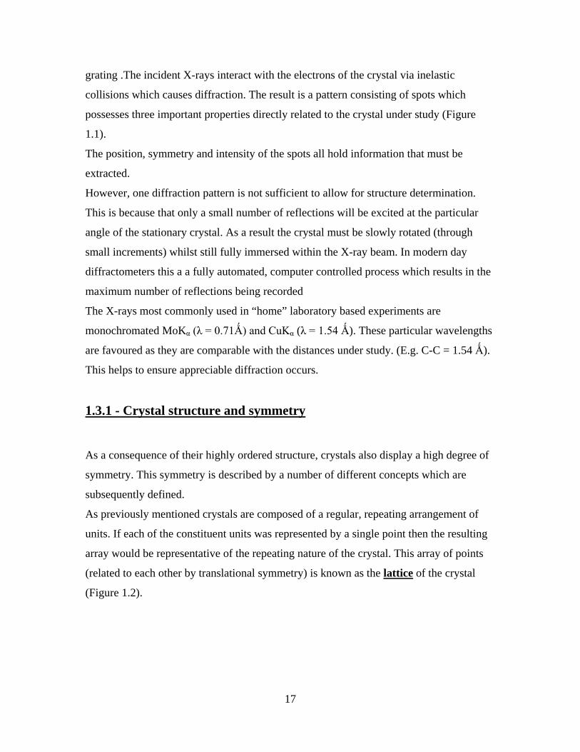
As previously mentioned crystals are composed of a regular, repeating arrangement of

units. If each of the constituent units was represented by a single point then the resulting

array would be representative of the repeating nature of the crystal. This array of points

(related to each other by translational symmetry) is known as the lattice of the crystal

(Figure 1.2).

18

Figure 1.2 – A demonstration of the crystal lattice, created by representing the

constituent units with points

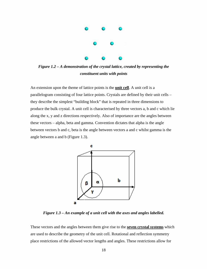
An extension upon the theme of lattice points is the unit cell. A unit cell is a

parallelogram consisting of four lattice points. Crystals are defined by their unit cells –

they describe the simplest “building block” that is repeated in three dimensions to

produce the bulk crystal. A unit cell is characterised by three vectors a, b and c which lie

along the x, y and z directions respectively. Also of importance are the angles between

these vectors – alpha, beta and gamma. Convention dictates that alpha is the angle

between vectors b and c, beta is the angle between vectors a and c whilst gamma is the

angle between a and b (Figure 1.3).

Figure 1.3 – An example of a unit cell with the axes and angles labelled.

These vectors and the angles between them give rise to the seven crystal systems which

are used to describe the geometry of the unit cell. Rotational and reflection symmetry

place restrictions of the allowed vector lengths and angles. These restrictions allow for

19

classification into seven groups – triclinic, monoclinic, orthorhombic, tetragonal, trigonal,

hexagonal and cubic. The aforementioned restrictions are given in Table 1.

Crystal system Unit cell restrictions Essential symmetry of crystal

Triclinic None None

Monoclinic One diad axis (2 fold rotation)

or mirror plane (inverse diad

axis)

a ≠ b ≠ c

β ≠ α = γ = 90°

Orthorhombic Three orthogonal diad axes or

inverse diad axes

a ≠ b ≠ c

α = β = γ = 90°

Tetragonal One tetra axis (four fold

rotation) or inverse tetrad axis

a = b = c

α = β = γ = 90°

Trigonal One triad (three fold rotation)

axis or inverse triad axis

a = b = c

α = β = γ ≠ 90°

Hexagonal One hexad (five fold rotation)

axis or inverse hexad axis

a = b ≠ c

α = β = 90°, γ = 120°

Cubic Four triad axes or inverse triad

axes

a = b = c

α = β = γ = 90°

Table 1 – The essential crystal symmetry and unit cell restrictions of the seven crystal

systems.

Introducing translational symmetry into the seven crystal systems (which only include

rotational and reflection symmetry) forms the Bravais (or space) lattices. There are 14

possible Bravais lattices which involve four different ways of centring the lattice points

(Figure 1.4). The possible lattice centrings are –

- Primitive (P) – Lattice points are located at the corners of the unit cell.

- Body Centred (I) – All primitive points included plus an additional point at the

centre of the unit cell.

- Face Centred (F) – All primitive points included plus additional points at the

centre of each face of the unit cell.

20

- Centred (C) – All primitive points included plus an additional point at the

centre of one face of the unit cell.

Figure 1.4 – The fourteen Bravais lattices with the lattice points displayed1.

A point group is a mathematical descriptor for a group of symmetry operations that pass

through a central point. These symmetry operations must leave at least one point

unchanged and the appearance of the object unaltered.

There are four symmetry operations associated with point groups -

- n-fold rotation axes – a rotation through (360°/n) which leaves the object

unaltered (where n is an integer).

- Mirror planes – involves a reflection which takes place with respect to a

mirror plane.

- Inversions – involves moving every point x,y,z to –x,-y,-z.

- Improper rotations - a rotation followed by an inversion.

Compared to the point groups for an isolated object (such as a single molecule) there are

230 possible crystallographic space groups. This is because there are 32 possible ways to

combine the point group symmetry operations with the translational symmetry inherently

present within crystals (crystallographic restriction theorem). For point groups the

Schoenflies notation is most commonly used. For example the molecule SF6 belongs to

21

the octahedral point group (in Schoenflies notation represented by Oh) which contains 31

associated symmetry elements2.

The specific method of describing the symmetry present in a crystal is that of space

groups. Space groups describe the symmetry operations present in an infinitely repeating

three dimensional pattern (crystals are as an approximation to infinite repeating

structures). Therefore each space group is a combination of the point group symmetry

operations with translational (or space) symmetry operations.

There are 230 space groups which completely describe all possible combinations of the

aforementioned symmetry operations.

Typically the internationally recognised Hermann and Magiun notation is used.

A typical example is P 21/m –Where P is the type of Bravais lattice – Primitive in this

example.

The letters following the P represent the symmetry operations which lie along a special

direction in the crystal. In this example 21 represents a 21 screw axis in the direction of

the unique axis of the monoclinic crystal system. The ‘/m’ represents an ordinary

reflection plane which is perpendicular to the unique 21 axis.

The space groups and their associated symmetry operations are systematically detailed in

the International Tables for Crystallography3.

In addition to the symmetry operations possessed by point groups there are two space

symmetry operations which may be contained within space groups. These operations are

termed glide planes and screw axes.

A screw axis is a combination of a rotation of (360/n) followed by an appropriate

translation parallel to the axis of rotation to preserve the translational repetition (where n

is an integer). For example a 21 screw axis consists of a twofold rotation axis (360°/2)

followed by a translation along half of the lattice axis that is parallel to the rotation

(Figure 1.5).

22

Figure 1.5 – The effect a 21 screw axis has upon a particular point4.

A glide plane is a combination of a reflection in a mirror plane followed by a translation.

There are five possible glide planes – denoted a, b, c, n and d. For example a c glide plane

consists of a reflection in the xy plane followed by a translation along half of the c axis.

Screw axes and glide planes can cause the systematic absence of certain reflections in a

diffraction pattern. These systematic absences can help in the assignment of space groups

as the absences are well known and are listed in the International Tables for

Crystallography3 (although space group ambiguities do exist).

1.3.2 - The Bragg equation

In 1913 W. L. Bragg derived his now eponymous equation5 following on from work

conducted by Freidrich, Knipping and Laue. This work proved a proposal by Laue which

was stimulated by Ewald that crystals were capable of diffracting X-rays. The Bragg

equation is still used today to mathematically explain the diffraction geometry of X-rays

by crystals.

The equation treats crystals as being composed of a series of parallel planes of atoms

separated by a small distance. The planes are assumed to be capable of reflecting the X-

rays in a manner which results in the angle of incidence equalling the angle of reflection

(Figure 1.6).

The contributions from successive planes will be in phase (i.e. the difference in path

length between successive waves must be an integer number of wavelengths) only for

certain angles.

As a result constructive interference and the production of diffraction maxima can only

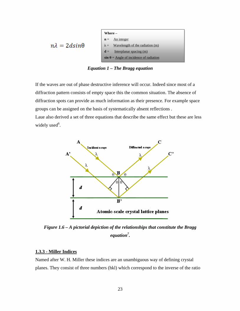
occur if the Bragg equation (Equation 1) is satisfied.

23

Equation 1 – The Bragg equation

If the waves are out of phase destructive inference will occur. Indeed since most of a

diffraction pattern consists of empty space this the common situation. The absence of

diffraction spots can provide as much information as their presence. For example space

groups can be assigned on the basis of systematically absent reflections .

Laue also derived a set of three equations that describe the same effect but these are less

widely used6.

Figure 1.6 – A pictorial depiction of the relationships that constitute the Bragg

equation7.

1.3.3 - Miller Indices

Named after W. H. Miller these indices are an unambiguous way of defining crystal

planes. They consist of three numbers (hkl) which correspond to the inverse of the ratio

Where –

n = An integer

λ = Wavelength of the radiation (m)

d = Interplanar spacing (m)

sin θ = Angle of incidence of radiation

24

of the intercepts on the a, b and c axes of the unit cell (for examples see Figures 1.7 &

1.8).

Figure 1.7 – A pictorial representation of the 111 Miller plane.

Figure 1.8 – A pictorial representation of the 010 Miller plane.

1.4.1 - Nature, production and detection of X-rays

X-rays are a form of electromagnetic radiation which possess wavelengths within the

range of 0.01nm (0.1 Ǻ) to 10nm (100 Ǻ) with wavelengths in the range 0.2 – 3 Ǻ being

useful in crystallography. As such they consist of an electric field and magnetic field

vector which are perpendicular to each other. These vectors oscillate in a sinusoidal

manner perpendicular to the direction of propagation.

X-rays are the favoured form of radiation in crystallography as they possess wavelengths

comparable to bond lengths and can also be easily generated in a “home” laboratory

setting. A more recent method of generating much more intense and finely tuneable X-

rays using a synchrotron source is also now widely used.

1.4.2 - X-ray tubes – For X-ray generation in the “home” laboratory

X

Y

Z

Y

X

Z

25

The X-ray tubes used in modern day crystallography are known as filament (or Coolidge)

tubes and date back to 1913. They consist of an evacuated glass enclosure which contains

a tungsten filament and a disk of a target metal (Figure 1.9). The target metal is

responsible for the production of the characteristic wavelength of the X-rays. The most

commonly used target metals are Molybdenum (wavelength = 0.71 Ǻ), Copper (1.54 Ǻ)

and Silver (0.56 Ǻ).

To initiate the production of X-rays the tungsten filament is heated by passing an electric

current through it. This results in the production of electrons which are accelerated by a

potential difference and directed towards the target metal. If the potential difference is

sufficiently high (typically 40kV) the electrons will possess enough energy to cause

ionisation of inner core electron`s of the target metal. To compensate an electron in a

higher atomic energy level for the metal will drop in energy to take the place of the

ejected electron. This results in the emission of a photon with a characteristic wavelength.

The characteristic wavelength produced is dependent upon the metal atom energy levels

from which each electron is ejected. For example MoKα emission corresponds to

electrons moving between the L and M shells (λ = 0.71Ǻ) of Molybdenum whilst MoKβ

emission corresponds to a movement between the L and K shells (λ = 0.63λ).

This characteristic wavelength created is defined by Equation 2.

Equation 2 – The equation for the characteristic wavelength generated from a

particular target material.

The spectra purity of the X-ray beam onto the crystal is created by using filters to remove

background and other unwanted wavelengths whilst a beryllium window allows the X-

rays to leave the tube head with minimum absorption.

Where –

h = Plancks constant (6.6261 x 10-34 J s)

c = Speed of light (2.9989 x 108 m/s)

E1 = Lower energy level of target atom

E2 = Higher energy level of target atom

26

This method of X-ray production can be considered quite inefficient as the vast majority

of the energy carried by the electrons is converted into heat rather than X-rays (literature

sources mention 1% X-ray conversion8). The heating of the target is largely compensated

by a water cooling system which prevents melting of the target material up to certain

current limits. An additional disadvantage of this method is that the X-rays generated are

quite divergent which may pose a problem if small crystals are under study.

Figure 1.9 – A schematic diagram of an X-ray tube9.

An improved method of generating X-rays in the home laboratory is known as a rotating

anode. In this apparatus the target metal is cylindrical and is spun about its axis. This

allows the energy of the X-rays to be spread out over a larger overall area thereby

reducing the heating problem. As a result much higher electrical currents can be

introduced which creates a much higher flux density. This method of X-ray generation is

important especially for molecules which possess large unit cells such as proteins which

are often in large complexes.

1.4.3 - Synchrotron source X-ray generation

Synchrotrons were initially developed as a tool in particle physics to accelerate beta

particles (electrons and positrons). It is observed that when such particles are accelerated

through magnetic fields at relativistic speeds they lose energy in the form of

electromagnetic radiation (this radiation covers the entire EM spectrum not just X-rays).

27

When the beta particles pass through the magnetic fields they change direction. This

causes the tangential emission of radiation. Although emission of radiation occurs at non

relativistic speeds, a feature of relativity known as the Lorentz transformation means that

the radiation is emitted in a highly collimated fashion at speeds approaching that of the

speed of light. This emission of radiation was first observed in 1946 at a 70MeV

synchrotron in Schenectady by F. R. Elder et al10. Today many synchrotron sources are

now operational as nationally and internationally shared facilities.

Synchrotrons consist of a linear accelerator (LINAC) which creates high energy electrons

(around 10MeV). These electrons are subsequently injected into a small accelerator

(known as a booster synchrotron) which increases the energy of the electrons to around

500MeV. Once this point has been reached the electrons are injected into the main

synchrotron ring where the energy is further increased via multiple passes through radio

frequency cavities. This produces X-rays which extends to the necessary short

wavelengths and are much more intense and well collimated than laboratory based

sources. This allows for extremely fast data collection times and smaller crystals to be

studied. The continuous spectrum allows for the fine tuning of the selected wavelengths

using monochromators. Alternatively the whole ‘white’ X-ray spectrum may be used in

Laue diffraction experiments.

1.4.4 - Detection of X-rays

In the beginnings of X-ray crystallography intensities were often measured by using

photographic films coated in silver halide. Exposure to X-rays causes silver halide to

darken. The darkness of the spots is related to the intensity of the absorbed radiation in a

given reflection (spot).

A vast improvement was the appearance of computer controlled diffractometers in the

1960`s. These routinely utilised an X-ray sensitive electronic device known as a

scintillation counter. A scintillation counter consists of a crystal mounted onto a

photomultiplier tube. A commonly used crystal is sodium iodide doped with a small

amount of Thallium (around 1%)11. These crystals produce light when irradiated by X-

rays. This light can then enter the photomultiplier which results in the ejection of

electrons and thus the generation of an electric current. This process results in the

28

production of an electric pulse for each individual X-ray allowing for the measurement of

intensities. There are disadvantages associated with scintillation counters. Foremost is

that the diffracted beams are measured one at a time which often translates to long data

collection times.

A more recently developed method of X-ray detection is known as a charge coupled

device (CCD). These detectors have the advantage of being able to record a number of

diffracted beams at the simultaneously, thereby reducing data collection times. A CCD

detector employs a semiconductor in which the incident X-rays induce the production of

free electrons and electron holes12. The electrons produced are trapped in potential wells,

and in addition to the electron holes, are read out as a current. The magnitude of this

current is proportional to the intensity of the diffracted beams .The various designs of

CCD detectors can be roughly divided into two groups depending on how the intensity of

the radiation is detected. This may be done by either measuring the intensity of the X-

rays directly or by conversion of the X-rays to visible light using a phosphor conversion

mechanism13.

Diffractometers that utilise a CCD detector are often known as three circle

diffractometers. This is because they possess three rotation axes (one in relation to the

detector and two in relation to the crystal). Scintillation counter based diffractometers

possess four rotation axes as the detector is smaller and can only record reflections which

occur in the horizontal plane. As a result an additional crystal rotation axes is required.

1.5 - Crystal growth

Crystals are formed as a result of chemical systems seeking to minimise the Gibbs free

energy. On the one hand the formation of crystals results in an unfavourable loss of

entropy. This arises because the individual molecules which constitute the crystal are in

effect “locked” in place. As a result they lose rotational and translational degrees of

freedom. Conversely this is coupled with a favourable increase in the enthalpy of a

system. This increase arises because the crystallisation process involves the formation of

many new, stable non covalent chemical bonds. This increase in enthalpy more than

29

counterbalances the unfavourable decrease in entropy and overall favourably decreases

the Gibbs free energy.

Small molecule and macromolecule crystal growth utilise different apparatus, although

common pricincples. The initial aim is to tailor the experimental conditions so that the

solution is just saturated. At this moment the saturation point should be very slowly

lowered whilst the rate of nucleation is limited. In theory this should yield well formed

and decently sized crystals possessing a high degree of regularity.

In practice however obtaining crystals of a suitable size and quality is often a major rate

limiting step in the structure determination process. The crystallisation process in a given

case is often poorly understood whilst the high number of variables involved (e.g.

temperature, pH, concentrations) further complicates the process. However there are

exceptions, for example the crystal growth of silicon is exceedingly well understood.

Techniques for inducing the crystallisation of small molecules are often much simpler

than those used in macromolecular crystallisation. Commonly used techniques to induce

small molecule crystallisation are the slow evaporation of a solution, slow precipitation

by vapour diffusion and sublimation.

Macromolecular crystallisation techniques are discussed in Chapter 5 although both areas

often use vapour diffusion (although the apparatus differs slightly as illustrated by

Figures 1.10 & 1.11).

Figure 1.10 – The vapour diffusion method for small molecule crystallisation.

30

Figure 1.11 – The hanging drop vapour diffusion method for macromolecular

crystallisation.

1.6.1 - Structure determination procedure

Once crystals of a suitable size have been grown the crystal structure determination

procedure can begin. This procedure can be thought of as being divided into three main

stages –

- The first stage involves the measurement of the intensities of the Bragg reflections

and the application of corrections to take into account various geometrical and

physical phenomena.

- The second stage involves using mathematical and computer program methods to

imitate the behaviour of a microscope lens to solve the phase problem.

- The final stage involves refining the initial structure so that there is an optimum

agreement between the observed and calculated structure factors.

The steps involved in each of these stages are further explained below.

1.6.2.1 - Stage 1 – Measurement of X-ray intensities

1.6.2.2 - Step 1 - The first step towards measuring X-ray intensities is the selection

and preparation of a suitable single crystal.

For use in home laboratory experiments single crystals in the order of 0.2-0.4mm are

routinely required. This is because the X-ray beam generated is relatively weak in

31

intensity (compared to a synchrotron source) and the diameter is less than 1mm; using

such a small size ensures that the crystal is fully immersed in the X-ray beam. It is

important to inspect crystals beforehand using a microscope to ensure that no visible

defects such as cracks or twinning are apparent. In addition crossed polarisers can be used

to ensure that the crystals extinguish. This can help to reveal defects within the crystal

that were previously not apparent. However should not be considered a conclusive test as

some crystals (depending upon their symmetry) do not extinguish.

Once a crystal of a suitable size and quality has been selected it can be mounted onto a

small loop or mesh (Figure 1.12). The crystal is held in place by using a small amount of

amorphous glue. If the data is to be collected at a cryogenic temperature then a viscous

oil can be used. The oil will freeze in the cryogenic stream thereby again fixing the

crystal in place. Data collection at cryogenic temperatures is advantageous as it reduces

the rate of radiation damage caused by the incident X-rays. In addition cryogenic

temperatures reduce atomic mobility which in turn enhances the diffraction spot

intensities (as this minimises disorder). In special cases such as if the sample is air

sensitive the crystal can be contained within a thin walled glass capillary. The glass has

an amorphous structure and hence does not appreciably contribute to the diffraction

pattern.

Finally, the loop, mesh or capillary containing the crystal is mounted onto a goniometer

head and placed onto the diffractometer. The goniometer head is a device that allows the

crystal to be easily centred in the X-ray beam. Additionally in modern day

diffractometers a high magnification video camera is used to ensure that the crystal is in

the correct position and to record a digital picture of the crystal for size determination.

32

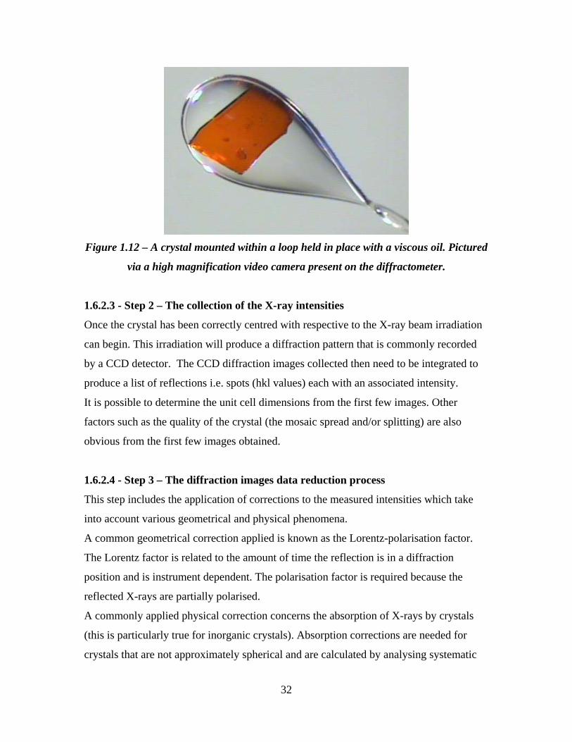
Figure 1.12 – A crystal mounted within a loop held in place with a viscous oil. Pictured

via a high magnification video camera present on the diffractometer.

1.6.2.3 - Step 2 – The collection of the X-ray intensities

Once the crystal has been correctly centred with respective to the X-ray beam irradiation

can begin. This irradiation will produce a diffraction pattern that is commonly recorded

by a CCD detector. The CCD diffraction images collected then need to be integrated to

produce a list of reflections i.e. spots (hkl values) each with an associated intensity.

It is possible to determine the unit cell dimensions from the first few images. Other

factors such as the quality of the crystal (the mosaic spread and/or splitting) are also

obvious from the first few images obtained.

1.6.2.4 - Step 3 – The diffraction images data reduction process

This step includes the application of corrections to the measured intensities which take

into account various geometrical and physical phenomena.

A common geometrical correction applied is known as the Lorentz-polarisation factor.

The Lorentz factor is related to the amount of time the reflection is in a diffraction

position and is instrument dependent. The polarisation factor is required because the

reflected X-rays are partially polarised.

A commonly applied physical correction concerns the absorption of X-rays by crystals

(this is particularly true for inorganic crystals). Absorption corrections are needed for

crystals that are not approximately spherical and are calculated by analysing systematic

33

variations in the intensities of symmetry related reflections. This is because the amount of

absorption is dependent upon the path length the X-rays travel through the crystal.

Absorption of X-rays also increases the larger the crystal is; using a crystal as small as

possible helps to minimise this error. Finally absorption varies with elemental

composition; often heavy atoms strongly absorb X-rays.

The data reduction process also involves the merging of symmetry related reflections and

the calculation and application of scale factors to the measured reflections. The result is a

unique, scaled data set. The data reduction process is a ‘black box’ method that is

performed by computers.

1.6.3.1 - Stage 2 – The crystallographic phase problem and possible

solutions The phase problem is intrinsic to X-ray crystallography. Each of the diffracted X-rays

will have a particular phase and amplitude associated with it. X-ray sensitive detection

methods such as photographic film or CCD detectors are able to measure intensities from

which the amplitudes are easily obtained (intensities = ampltiude2). However the relative

phases of the waves are lost during the experiment. This is a problem because in order to

elucidate the crystal structure both the intensities and relative phases are required.

Therefore a method of obtaining approximate phases and hence solving the phase

problem is required. In small molecule crystallography two methods are almost

exclusively used which both utilise a branch of mathematics known as Fourier series.

Fourier series arise from Fourier’s theorem which states that any periodic function can be

represented by a summation of sine and cosine terms. The diffraction pattern and the

electron density of a crystal are related by a Fourier series. In addition a diffraction

pattern consists of well defined individual spots. Therefore a summation must be used as

opposed to integration which would be performed if the pattern was diffuse.

Crystals can be described by a Fourier series as the structure of a crystal is a periodically

repeating, (effectively) infinite array.

34

The structure factor equation is used to describe how the incident X-rays are diffracted by

the constituent atoms of a crystal. This equation takes into account the scattering power

of each atom (which is described by fj which is the scattering factor for the jth atom) and

is dependent upon electron density. This is described by Equation 3.

Equation 3 – The structure factor equation.

The electron density calculation must be performed in three dimensions in order for a

three dimensional structure to be produced. The unit cell volume (V) must also be taken

into account. The equation used to calculate the electron density at a particular point

(xyz) is given by Equation 4.

Equation 4 – The equation used to calculate the electron density at point ρ(xyz).

The two commonly used methods used to solve the phase problem in small molecule

crystallography are described below.

1.6.3.2 – The Patterson Synthesis

This method is commonly employed when there is one or a small number of heavy atoms

present in the structure.

In 1934 A. L. Patterson presented a synthesis (or Patterson map) that is obtained by

performing a Fourier series on the square of the amplitudes with all waves taken in

Where –

N = The number of atoms

within the structure

fj = Atomic scattering factor

for the jth atom

35

phase14. If there are an N number of atoms in a unit cell then there is a N2 number of

vectors running between these atoms. Therefore a Patterson map shows where atoms are

located relative to each other but not where they are located with respective to the unit

cell origin. The result is a map that has an appearance similar to that of an electron

density map in that it contains peaks of positive density located in particular positions.

However this is not a map of electron density, instead it is a map of the vectors between

pairs of atoms in the structure. The Patterson synthesis is described mathematically by

Equation 5.

Equation 5 – The mathematical representation of the Patterson synthesis.

1.6.3.3 – Direct Methods

This method was developed for equal atom structures i.e. those that contain no heavy

atoms.

Direct methods also use the measured intensities but takes advantage of the fact that

electron density within a crystal can not be negative. This places restrictions on the

possible phase angles between reflections. The process is almost a trial and error

approach – the reflections which contribute most to the Fourier transform are selected as

are approximations that appear promising (assessed by a numerical factor). The Fourier

series are calculated using the measured intensities and these approximate phases.

Sensible looking chemical fragments can be used to assess the different trial structures.

The resulting trial structure is only an initial approximation of the true structure and must

undergo further refinement.

Direct methods are often described as black box as the process is automated and

performed by computers.

Where –

V = The unit cell volume

(in Ȧ3).

36

Methods used to solve the phase problem in macromolecular crystallography differ and

are detailed in Chapter 5.

1.6.4 - Stage 3 – Refining the structure The final stage involves refining the initial structure so that there is a optimum agreement

between the observed structure factor amplitudes and the structure factor amplitudes

calculated for the current structure.

The measure by which these factors agree is described by the conventional residual factor

(commonly known as the R factor). The R factor is defined by Equation 6.

Equation 6 – The conventional residual factor.

As illustrated by Equation 6 the lower the R factor the better the agreement and the more

correct the structure is. That the earlier stages of the structure determination procedure

were performed correctly is essential if a low R factor is to be obtained.

Refinement uses a mathematical technique known as least squares analysis which adjusts

parameters such as atom positions and atomic displacement parameters in order to

produce the maximum agreement between two sets of data (in this case the observed and

calculated amplitudes). The refinement on F2 was used in this thesis and is defined by

Equation 7.

Where –

FO = Observed structure factor amplitude

FC= Calculated structure factor amplitude from model

Where –

yO = Observed structure factor amplitude

yC= Calculated structure factor amplitude from model

37

Equation 7 – The least squares refinement of the square of the structure factor

amplitudes.

Several cycles of refinement are required as the data used is calculated using Fourier

series which are non linear equations. Consequently cycles of refinement are required

until the adjustments of the parameters are insignificant (a process known as

convergence).

The refinement parameters can be split into two groups based on the mathematical detail

used to describe the atoms. Isotropic refinement uses three positional coordinates (x,y,z)

as well as a single vibrational parameter to approximate vibrating atoms as spheres.

Anisotropic refinement uses the same three positional coordinates as well as six

vibrational parameters to describe atoms in terms of ellipsoids. Although a perfect

ellipsoid can be described by three vibrational parameters atoms typically possess

distorted ellipsoids which are described by require six vibrational parameters .This results

in a significantly more accurate and realistic model structure. In addition, once

anisotropic refinement has been carried out small peaks can often be observed,

corresponding to hydrogen atom positions.

The process of refinement is complete when convergence is achieved and the electron

density map contains no undefined peaks or holes.

For small molecule X-ray crystallography a final R factor in the range 0.02 – 0.07 is an

indicator of a good quality structure.

38

Chapter 2

Structure determination of a small molecule – C26H36N8018Cl2Co

2.1 - Introduction to C26H36N8O18Cl2Co

This complex was synthesised by the group of Professor Subrata Mukhopadhyay of the

University of Jadavpur, India for study into the field of crystal engineering. The field of

crystal engineering seeks to utilise intermolecular interactions to aid molecular

recognition through the identification and control of recognition motifs. The field is still

relatively new and its full potential has yet to be realised. This is because there are

problems present which are poorly understood, for example weak interactions can prove

especially unpredictable and therefore difficult to control. However it is hoped that

molecular recognition may prove useful in the design and synthesis of future functional

materials.

In order for molecular recognition to be successfully implemented a full appreciation of

the intermolecular interactions present is required. This can be achieved using single

crystal X-ray crystallography to provide a complete unambiguous three dimensional

structure.

The probable composition of the complex was determined by the synthetic chemists as

[Co(mal)2(H2O)2](ClO4)2(LH)4 where mal indicates malonate and LH4 indicates

protonated 2-amino pyridine.

2.2 – X-ray diffraction data collection and processing procedure

The crystals provided were approximately 1-2 mm in length and pink in colour. The

crystals appeared to be of good quality and extinguished well under crossed polarisers.

As a result a single crystal was cut using a razor blade to around 0.5mm in length. The

crystal was then immersed in a viscous oil and fitted onto a loop, which was placed onto

a goniometer head and fitted onto the diffractometer. The data collection was performed

39

at a cryogenic temperature (100K), which caused freezing of the viscous oil and thus

fixation of the crystal. This is in addition to being beneficial by reducing atomic

displacement parameters. The crystal was centred using rotating screws on the

goniometer head and a video camera as a visual aide. Firstly the X-axis was adjusted at

phi 0˚ to ensure the crystal was centred. Once complete the screw was rotated to phi 180˚

and the crystal centred again. This process was repeated in the same manner for the Y-

axis but with phi angles 90˚ and 270˚. Once the crystal was completely centred it was

irradiated with monochromated MoKα radiation. The X-ray generator settings were 40kV

and 40 mA.

The computer program SAINT15 was used to collect and integrate the CCD frame images

in order to produce integrated intensities. This produced files with filename extensions

.p4p and .RAW. These files were then introduced into SHELX16 XPREP for

determination of the crystal system and space group. SHELX SADABS was used to

produce an X-ray absorption corrected data set which took into account absorption of X-

rays by the crystal, although this was a symmetrically sized crystal (crystal dimensions

listed in Table 2).

It was found that SHELX XS was unable to satisfactorily solve the structure using both

direct methods or a Patterson synthesis. This sort of unexplained failure of SHELX can

occur. As a result the direct methods program SIR 200417 was used to solve the structure.

Further refinement was carried out within the SHELX XSHELL program.

All non hydrogen atom positions were refined anisotropically. The hydrogen atom

positions were clearly visible using difference Fourier methods and were refined

isotropically.

Empirical formula C26H36N8018Cl2Co

Chemical formula weight 878.46 g mol-1

Crystal system Triclinic

Space group P 1

40

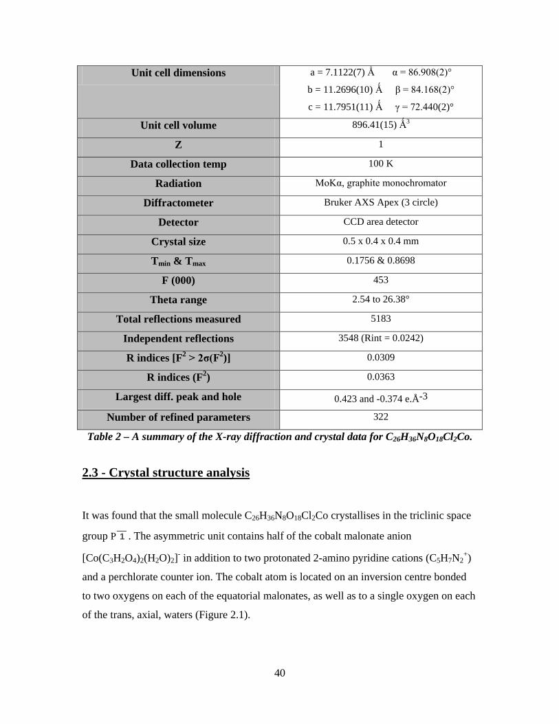
Unit cell dimensions a = 7.1122(7) Ǻ α = 86.908(2)°

b = 11.2696(10) Ǻ β = 84.168(2)°

c = 11.7951(11) Ǻ γ = 72.440(2)°

Unit cell volume 896.41(15) Ǻ3

Z 1

Data collection temp 100 K

Radiation MoKα, graphite monochromator

Diffractometer Bruker AXS Apex (3 circle)

Detector CCD area detector

Crystal size 0.5 x 0.4 x 0.4 mm

Tmin & Tmax 0.1756 & 0.8698

F (000) 453

Theta range 2.54 to 26.38°

Total reflections measured 5183

Independent reflections 3548 (Rint = 0.0242)

R indices [F2 > 2σ(F2)] 0.0309

R indices (F2) 0.0363

Largest diff. peak and hole 0.423 and -0.374 e.Å-3

Number of refined parameters 322

Table 2 – A summary of the X-ray diffraction and crystal data for C26H36N8O18Cl2Co.

2.3 - Crystal structure analysis

It was found that the small molecule C26H36N8O18Cl2Co crystallises in the triclinic space

group P 1 . The asymmetric unit contains half of the cobalt malonate anion

[Co(C3H2O4)2(H2O)2]- in addition to two protonated 2-amino pyridine cations (C5H7N2+)

and a perchlorate counter ion. The cobalt atom is located on an inversion centre bonded

to two oxygens on each of the equatorial malonates, as well as to a single oxygen on each

of the trans, axial, waters (Figure 2.1).

41

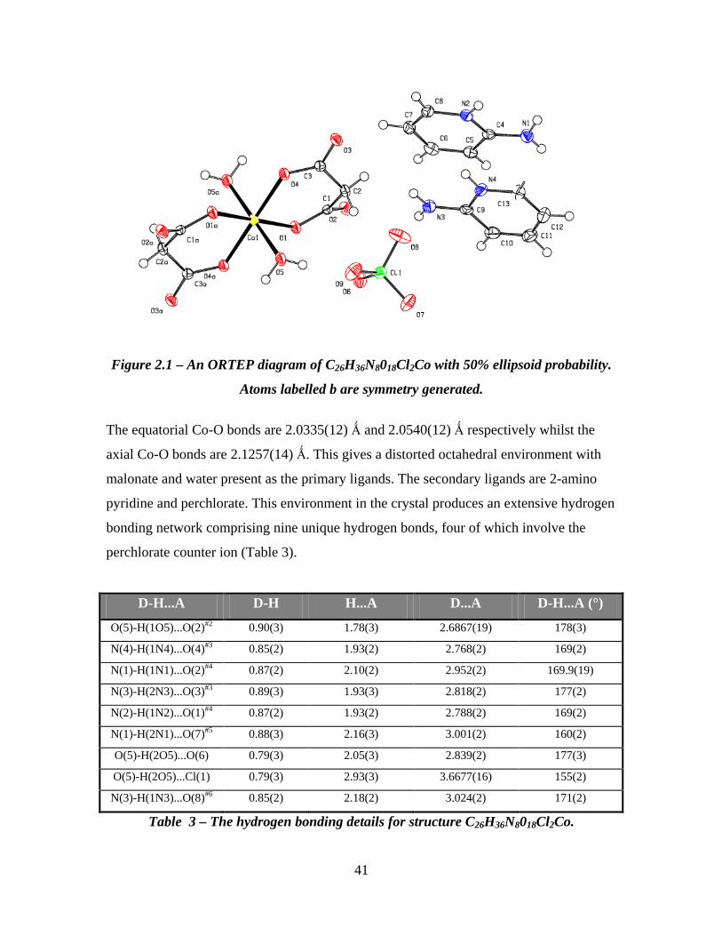
Figure 2.1 – An ORTEP diagram of C26H36N8018Cl2Co with 50% ellipsoid probability.

Atoms labelled b are symmetry generated.

The equatorial Co-O bonds are 2.0335(12) Ǻ and 2.0540(12) Ǻ respectively whilst the

axial Co-O bonds are 2.1257(14) Ǻ. This gives a distorted octahedral environment with

malonate and water present as the primary ligands. The secondary ligands are 2-amino

pyridine and perchlorate. This environment in the crystal produces an extensive hydrogen

bonding network comprising nine unique hydrogen bonds, four of which involve the

perchlorate counter ion (Table 3).

D-H...A D-H H...A D...A D-H...A (°)

O(5)-H(1O5)...O(2)#2 0.90(3) 1.78(3) 2.6867(19) 178(3) N(4)-H(1N4)...O(4)#3 0.85(2) 1.93(2) 2.768(2) 169(2)

N(1)-H(1N1)...O(2)#4 0.87(2) 2.10(2) 2.952(2) 169.9(19)

N(3)-H(2N3)...O(3)#3 0.89(3) 1.93(3) 2.818(2) 177(2)

N(2)-H(1N2)...O(1)#4 0.87(2) 1.93(2) 2.788(2) 169(2)

N(1)-H(2N1)...O(7)#5 0.88(3) 2.16(3) 3.001(2) 160(2)

O(5)-H(2O5)...O(6) 0.79(3) 2.05(3) 2.839(2) 177(3)

O(5)-H(2O5)...Cl(1) 0.79(3) 2.93(3) 3.6677(16) 155(2)

N(3)-H(1N3)...O(8)#6 0.85(2) 2.18(2) 3.024(2) 171(2)

Table 3 – The hydrogen bonding details for structure C26H36N8018Cl2Co.

42

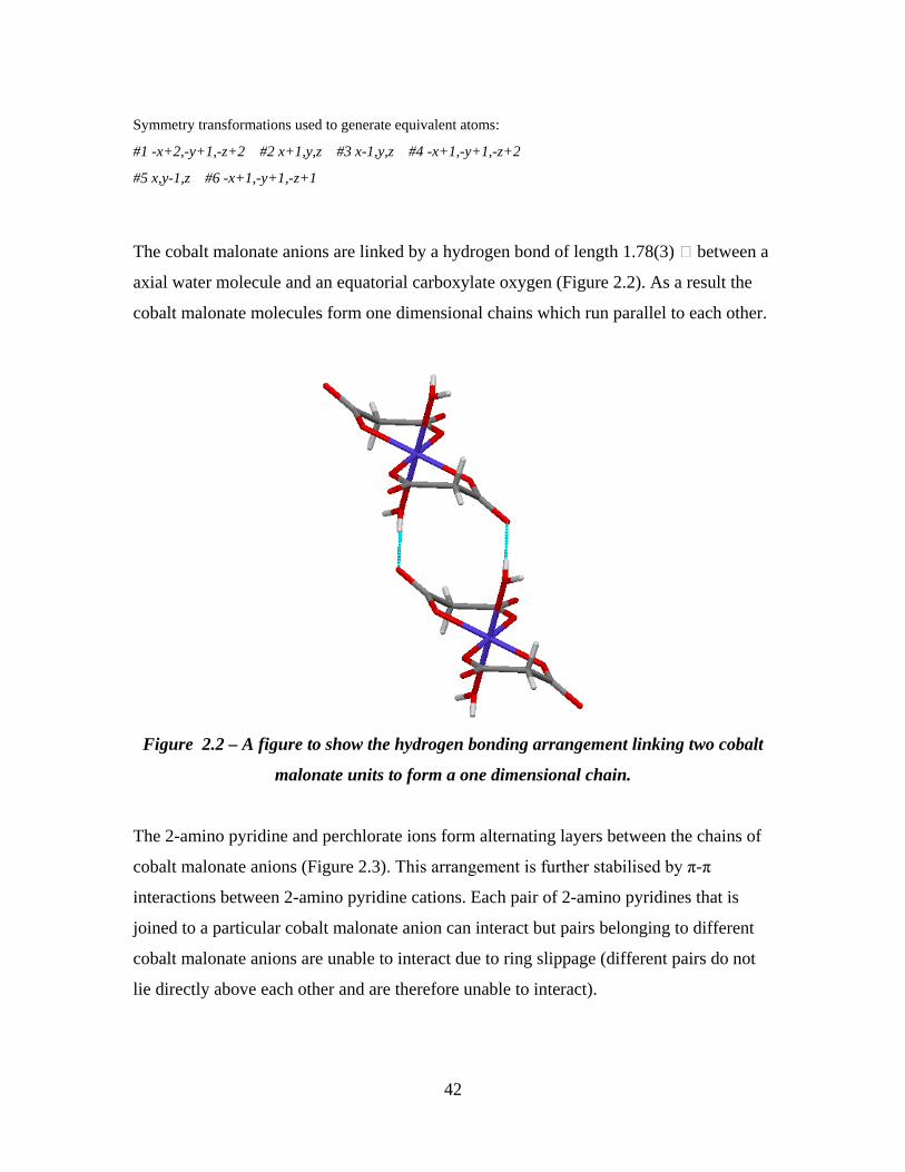
Symmetry transformations used to generate equivalent atoms:

#1 -x+2,-y+1,-z+2 #2 x+1,y,z #3 x-1,y,z #4 -x+1,-y+1,-z+2

#5 x,y-1,z #6 -x+1,-y+1,-z+1

The cobalt malonate anions are linked by a hydrogen bond of length 1.78(3) Ȧ between a

axial water molecule and an equatorial carboxylate oxygen (Figure 2.2). As a result the

cobalt malonate molecules form one dimensional chains which run parallel to each other.

Figure 2.2 – A figure to show the hydrogen bonding arrangement linking two cobalt

malonate units to form a one dimensional chain.

The 2-amino pyridine and perchlorate ions form alternating layers between the chains of

cobalt malonate anions (Figure 2.3). This arrangement is further stabilised by π-π

interactions between 2-amino pyridine cations. Each pair of 2-amino pyridines that is

joined to a particular cobalt malonate anion can interact but pairs belonging to different

cobalt malonate anions are unable to interact due to ring slippage (different pairs do not

lie directly above each other and are therefore unable to interact).

43

Figure 2.3 – A figure to show the crystal packing arrangement of C26H36N8018Cl2Co .

The 2-amino pyridine and perchlorate molecules form alternating layers between the

parallel cobalt malonate chains.

2.4 - Crystal structure implications

The structure was solved with a low R factor of 0.031 (as described by Equation 6) and

was consistent with the expected chemical composition.

The presence of the electron accepting oxygen and chlorine atoms of the perchlorate

anion help in the formation of an extensive hydrogen bonding network in the crystal.

Further stabilisation is provided via π-π interactions between aromatic rings of the 2-

amino pyridine cations. These intermolecular interactions help to minimise the free

energy by decreasing the enthalpy and therefore help promote crystallisation.

44

Chapter 3

Structure determination of a small molecule – C26H36N8O10F12P2Co

3.1 Introduction to C26H36N8O10F12P2Co

Presented in this chapter is the data collection procedure and structural analysis of a

cobalt containing complex. This complex was again synthesis by the group of Professor

Subrata Mukhopadhyay of the University of Jadavpur, India, for study into the field of

crystal engineering. The complex and the previous example were expected to be closely

related with both expected to contain 2-amino pyridine and malonate ions.

The probable composition of the complex was determined by the synthetic chemists as

[Co(mal)2(H2O)2](PF6)2(LH)4 where mal indicates malonate and LH4 indicates protonated

2-amino pyridine.

3.2 – X-ray diffraction data collection and processing procedure

The crystals provided were pink in colour and had an average size of approximately 5mm

to 1cm in length. The crystals appeared to be of good quality and extinguished well under

crossed polarisers. As a result a single crystal was cut using a razor blade to around

0.3mm in length. The crystal was then immersed in a viscous oil then fitted and mounted

as described in chapter 2. Once centred the crystal was irradiated with monochromated

MoKα radiation. The X-ray generator settings were 40 kV and 40 mA.




determination of the crystal system and space group. SHELX SADABS was used to

produce an absorption corrected data set which took into account absorption of X-rays by

the crystal, although this was a symmetrically sized crystal (crystal dimensions listed in

45

Table 4). The direct methods program SHELX XS was used to solve the structure with

further refinement being performed in the SHELX XSHELL program



isotropically.

Empirical formula C26H36N8O10F12P2Co



Space group P 1

Unit cell dimensions a = 7.1433(5) Ǻ α = 84.3130(10)°

b = 11.7421(9) Ǻ β = 84.2630(10)°

c = 11.8894(9) Ǻ γ = 72.3190(10)°

Unit cell volume 9421.90(12) Ǻ3

Z 1

Data collection temp 100K





Tmin & Tmax 0.7328 & 0.8788

F (000) 493



Independent reflections 4299

R indices [F2 > 2σ(F2)] 0.0313


Largest diff. peak and hole 0.502 and -0.276 e.Å-3


Table 4– A summary of the X-ray diffraction and crystal data for C26H36N8O10F12P2Co.

46

3.3 - Crystal structure analysis

It was found that the small molecule C26H36N8O10F12P2Co crystallises in triclinic space

group P 1 . The asymmetric unit contains half of the cobalt malonate anion

[Co(C3H2O4)2(H2O)2]- in addition to two protonated 2-amino pyridine cations (C5H7N2+)

and a PF6 counter ion (Figure 3.1). Like the previous structure the cobalt atom is located

on an inversion centre bonded to two oxygens on each of the equatorial malonates as well

as to a single oxygen on each of the trans axial waters.

Figure 3.1– An ORTEP diagram of C26H36N8O10F12P2Co with 50% ellipsoid

probability. Atoms labelled b are symmetry generated.

The equatorial Co-O bonds are 2.03275(10) Ǻ and 2.0554(10) Ǻ respectively whilst the

axial Co-O bonds are 2.1232(12) Ǻ . This gives a distorted octahedral environment with

malonate and water present as the primary ligands. The secondary ligands are 2-amino

pyridine and PF6. Again this environment in the crystal gave rise to an extensive

hydrogen bonding network comprising of nine unique hydrogen bonds, four of which

involve the PF6 counter ion (Table 5).

D-H…A D-H (Ǻ) H…A (Ǻ) D…A (Ǻ) D-H…A (º)

N(4)-H(1)…O(1) 0.83(2) 2.01(2) 2.8286(16) 167.1(18)

47

N(3)-H(2)...O(2) 0.85(2) 2.10(2) 2.9409(17) 175(2)

N(3)-H(1)...F(4) 0.89(2) 2.12(2) 2.9828(16) 162.6(18)

N(2)-H(1)...O(4) 0.84(2) 1.93(2) 2.7737(17) 176(2)

N(1)-H(2)...F(1) 0.83(2) 2.13(2) 2.9238(18) 161(2)

N(1)-H(1)...O(3) 0.86(2) 1.96(2) 2.8155(19) 171(2)

O(5)-H(2)...O(2) 0.80(3) 1.88(3) 2.6737(16) 172(2)

O(5)-H(1)...F(2) 0.78(2) 2.36(2) 3.0681(19) 152(2)

O(5)-H(1)...F3 0.78(2) 2.24(2) 2.9381(17) 149(2)

Table 5 – The hydrogen bonding details for structure C26H36N8O10F12P2Co.

Like the previous crystal structure the cobalt malonate anions are linked by a hydrogen

bond of length 1.88(3) Ǻ between a axial water and a equatorial carboxylate oxygen

(Figure 2.2). The cobalt malonate anions form one dimensional chains which run parallel

to each other. The 2-amino pyridine and PF6 ions form alternating layers between the

chains (Figure 3.2).

This arrangement is further stabilised by π-π interactions between 2-amino pyridine

cations. Each pair of 2-amino pyridines that is joined to a particular cobalt malonate

anion can interact but pairs belonging to different cobalt malonate anions are unable to

interact due to ring slippage (different pairs do not lie directly above each other and are

therefore unable to interact).

Figure 3.2– A figure to show the crystal packing arrangement of C26H36N8O10F12P2Co

. The 2-amino pyridine and PF6 molecules form alternating layers between the parallel

cobalt malonate chains.

48

3.4 - Crystal structure implications

The structure was solved with a low R factor of 0.031 (as described by Equation 6) and

was consistent with the expected composition.

The presence of the electron accepting fluorine atoms of the PF6 anion help in the

formation of an extensive hydrogen bonding network. Further stabilisation is provided

via π-π interactions between aromatic rings of the 2-amino pyridine cations. These

interactions help to minimise the free energy by decreasing the enthalpy and therefore

allowing crystallisation to occur.

3.5 - Comparison of the crystal structures

X-ray analysis revealed that the crystal structures are closely isomorphous. It was found

that both crystallised in triclinic P 1 space group with almost identical atomic

arrangements and unit cell dimensions.

Due to the similar atomic composition and arrangement both structures contained a

common hydrogen bonding motif composed of 2-amino pyridine and cobalt malonate

molecules (Figure 3.3) which accounted for five of the nine bonds present within the two

structures.

49

Figure 3.3 – A figure illustrating the common hydrogen bonding motif which is present

in both structures C26H36N8O18Cl2Co and C26H36N8O10F12P2Co .

Differences arise when the hydrogen bonding arrangements around the respective counter

ions are examined (Figure 3.4). In the crystal structure of C26H36N8O18Cl2Co the central

chorine of the perchlorate molecule is involved in hydrogen bonding. However in the

crystal structure of C26H36N8O10F12P2Co the central phosphorous of the counter ion is not

involved in the hydrogen bonding network. This may be expected due to the difference in

electro negativity between the two atoms (phosphorus has a value of 2.19 whilst chlorine

has a value of 3.16 on the Pauling scale of electro negativity).

In addition the respective counter ions form hydrogen bonds with different ions. As

illustrated the perchlorate counter ion forms hydrogen bonds with two 2-amino pyridine

cations and two hydrogen bonds with a malonate anion (the chlorine to malonate

interaction is not pictured).

In comparison the PF6 counter ion forms hydrogen bonds with three 2-amino pyridine

cations and only one hydrogen bond with the cobalt malonate anion.

The lengths of the hydrogen bonds between the two structures are comparable except for

the case involving the chlorine atom of the perchlorate. This bond is anomalously long in

comparison to the others at 2.93(3) Ǻ with the remaining hydrogen bonds in the two

50

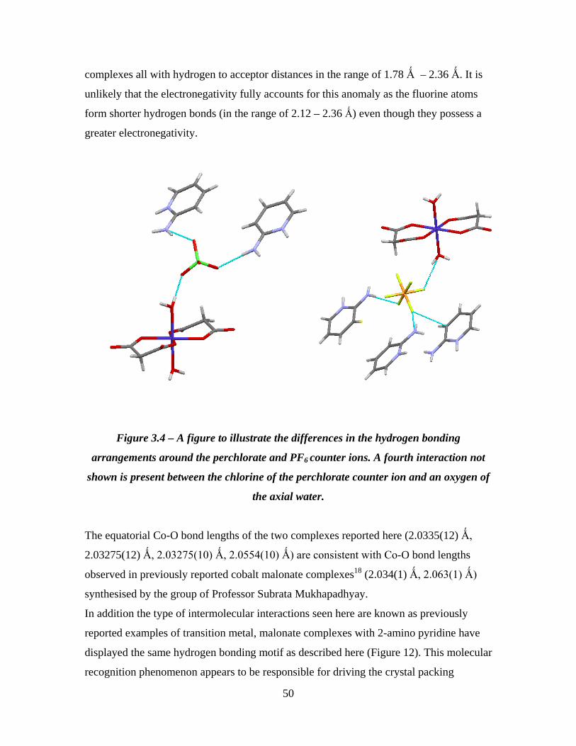
complexes all with hydrogen to acceptor distances in the range of 1.78 Ǻ – 2.36 Ǻ. It is

unlikely that the electronegativity fully accounts for this anomaly as the fluorine atoms

form shorter hydrogen bonds (in the range of 2.12 – 2.36 Ǻ) even though they possess a

greater electronegativity.

Figure 3.4 – A figure to illustrate the differences in the hydrogen bonding

arrangements around the perchlorate and PF6 counter ions. A fourth interaction not

shown is present between the chlorine of the perchlorate counter ion and an oxygen of

the axial water.

The equatorial Co-O bond lengths of the two complexes reported here (2.0335(12) Ǻ,

2.03275(12) Ǻ, 2.03275(10) Ǻ, 2.0554(10) Ǻ) are consistent with Co-O bond lengths

observed in previously reported cobalt malonate complexes18 (2.034(1) Ǻ, 2.063(1) Ǻ)

synthesised by the group of Professor Subrata Mukhapadhyay.

In addition the type of intermolecular interactions seen here are known as previously

reported examples of transition metal, malonate complexes with 2-amino pyridine have

displayed the same hydrogen bonding motif as described here (Figure 12). This molecular

recognition phenomenon appears to be responsible for driving the crystal packing

51

arrangement in the solid state. Formation of this motif apparently requires the presence of

2-amino pyridine. Previous work by the by the group of Professor Subrata

Mukhapadhyay found no such motif was formed when 4-amino pyridine was used in

place of 2-amino pyridine18.

The hydrogen bond lengths reported here are consistent with those previously reported

cobalt malonate complexes. However differences arise due to the presence of the

perchlorate and PF6 counter ions. It appears that introducing varying counter ions into the

complex can subtly alter the hydrogen bonding arrangement and therefore the crystal

packing arrangement. This may hold useful implications for crystal engineering where

the tight control of intermolecular interactions is essential.

52

Chapter 4

Structure Determination of two Small Molecules – C30H24NO4Sn &

C24H20Sn (SnPh4)

4.1 - Introduction to C30H24NO4Sn & C24H20Sn (SnPh4)

A set of two tin containing, crystalline compounds were submitted to the university by a

Pakistani research group for structure determination. The two compounds were expected

to be closely related. The expected chemical structures were determined by synthetic

chemists with the predicted structures shown in Figures 4.1 & 4.2.

Sn OO

NH

CF3

Figure 4.1 – The expected chemical structure of the molecule in the crystal MHB7.

Sn OO

NH

OCH3

Figure 4.2 – The expected chemical structure of the molecule in the crystal MHB8.

Sample MHB7 consisted of colourless, needle shaped crystals which were extremely thin

(around 0.08mm across). In contrast sample MHB8 consisted of colourless, block shaped

crystals with fairly symmetric dimensions. Both samples appeared to be of good quality

when viewed under a microscope and both extinguished well under crossed polarisers.

53

4.2 – X-ray diffraction data collection and processing procedure for

C24H20Sn (SnPh4)

Sample MHB7 was the first to be analysed. A single needle shaped crystal measuring

approximately 0.30 x 0.08 x 0.08mm was selected and immersed in a viscous oil. The

crystal was fitted on a loop, which was then placed onto a goniometer head and fitted

onto the diffractometer. The data collection was performed at a cryogenic temperature

(100K), which caused freezing of the viscous oil and thus fixation of the crystal as well as

being beneficial to reduce atomic displacement parameters. The crystal was centred using

rotating screws on the goniometer head and a video camera as a visual aide. Firstly the X-

axis was adjusted at phi 0˚ to ensure the crystal was centred. Once complete the screw

was rotated to phi 180˚ and the crystal centred again. This process was repeated in the

same manner for the Y-axis but with phi angles 90˚ and 270˚. Once the crystal was

completely centred it was irradiated with monochromated MoKα radiation. The X-ray

generator settings were 40kV and 40 mA.

After a sufficient number of frames had been collected using the SAINT15 computer

program the unit cell dimensions were determined (using the SMART15 computer

program) whilst data collection was still continuing. It was found that the dimensions of

the unit cell were 12.0079(14) x 12.0079(14) x 6.3934(16)Ǻ with angles 90 x 90 x 90˚.

These dimensions correspond to a tetragonal crystal system, which is fairly unusual for

small molecules (most small molecules crystallise in monoclinic or triclinic). A search of

the unit cell dimensions and space group of the Cambridge Crystallographic Data Centre

(CCDC) 19 using CONQUEST20 software revealed the dimensions to correspond to

SnPh4. This compound was used as a starting material in the synthesis and typically

forms needle shaped crystals.

Empirical formula C24H20Sn


Crystal system Tetragonal

54

Space group P 4 21/c

Unit cell dimensions a = 12.0079(14) Ǻ α = 90.00 ° b = 12.0079(14) Ȧ β = 90.00 ° c = 6.3934(16) Ȧ γ = 90.00 °

Unit cell volume 921.9(3) Ǻ 3

Z 2

Data collection temp 100 K





Tmin & Tmax 0.6808 & 0.8971

F (000) 428




R indices [F2 > 2σ(F2)] 0.0353


Largest diff. peak and hole 0.564 and -0.365 e.Ǻ-3


Table 6 – Summary of the X-ray diffraction data and refinement for C24H20Sn. The computer program SAINT was used to collect and integrate the CCD frame images



determination of the crystal system and space group. As the crystal contained a heavy tin

atom X-ray absorption corrections were applied using SHELX SADABS. These

corrections were also required because the crystal had quite unsymmetrical dimensions

(crystal dimensions listed in Table 6). The direct methods program SHELX XS was used

to solve the structure with further refinement being performed in the SHELX XSHELL

program.

55



isotropically.

4.3 - X-ray diffraction data collection and processing procedure for

C30H24NO4Sn

Sample MHB8 was subsequently analysed. A single colourless, block shaped crystal

measuring approximately 0.40 x 0.30 x 0.30mm was selected and mounted as described

for the previous crystal (Chapter 4.2). Once the crystal was completely centred it was

irradiated with monochromated MoKα radiation. The X-ray generator settings were 40kV

and 40 mA.



.p4p and .RAW. These files were then introduced into SHELX16XPREP for

determination of the crystal system and space group. Although this was a symmetrical

sized crystal (crystal dimensions listed in Table 7) the presence of a heavy tin atom

required the application of X-ray absorption corrections to the data set, which was done

using SHELX SADABS

The direct methods program SHELX XS was used to solve the structure with further

refinement being performed in the SHELX XSHELL program.



isotropically.

Empirical formula C30H24NO4Sn



Space group P 1

Unit cell dimensions a = 9.7556(5) Ǻ α = 73.1870(10) °

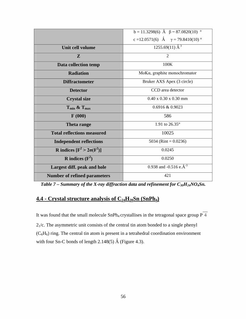
56

b = 11.3298(6) Ǻ β = 87.0820(10) ° c =12.0571(6) Ǻ γ = 79.8410(10) °

Unit cell volume 1255.69(11) Ǻ 3

Z 2

Data collection temp 100K





Tmin & Tmax 0.6916 & 0.9023

F (000) 586




R indices [F2 > 2σ(F2)] 0.0245


Largest diff. peak and hole 0.938 and -0.516 e.Ǻ-3


Table 7 – Summary of the X-ray diffraction data and refinement for C30H24NO4Sn.

4.4 - Crystal structure analysis of C24H20Sn (SnPh4) It was found that the small molecule SnPh4 crystallises in the tetragonal space group P 4

21/c. The asymmetric unit consists of the central tin atom bonded to a single phenyl

(C6H6) ring. The central tin atom is present in a tetrahedral coordination environment

with four Sn-C bonds of length 2.148(5) Ǻ (Figure 4.3).

57

Figure 4.3 – An ORTEP diagram of C24H20Sn with 50% ellipsoid probability. Atoms

labelled a,b or c are symmetry generated.

Using both the PLATON21 and SHELX computer programs it was found that no classical

hydrogen bonds were present within the crystal structure. This is due to the complete

absence of both suitable hydrogen bond donors and acceptors. There is however the

presence of weak van der Waals interactions (between carbon and hydrogen atoms) with

each SnPh4 molecule forming eight weak interactions (Figure 4.4) with eight other

neighbouring SnPh4 molecules.

58

Figure 4.4 – A figure to show the location of eight weak H…C-H interactions that each

C24H20Sn molecule forms.

It is found that the aromatic phenyl rings do not lie above each other in the crystal

packing arrangement. The adopted arrangement prevents the aromatic phenyl rings

interacting with each other via π-π stacking (Figure 4.5).

Figure 4.5 – A figure to show the stacking of the C24H20Sn molecule within the crystal.

Such an arrangement prevents the formation of π-π interactions.

59

Instead the molecules appear to form layers that are stabilised by the weak H…C-H

interactions running between them (Figure 4.6).

Figure 4.6 – A figure to show the stacking of layers of C24H20Sn molecules stabilised by

weak van der Waals interactions.

4.5 - Crystal structure analysis of C30H24NO4Sn

It was found that the small molecule C30H24NO4Sn crystallises in the triclinic space group

P 1 . The asymmetric unit contains two molecules of C30H24NO4Sn, which are joined to

each other via a O-Sn bond.

60

Figure 4.7 – An ORTEP diagram of C30H24NO4Sn with 50% ellipsoid probability.

Atoms labelled a or b are symmetry generated.

Using PLATON21 to analyse the crystal structure the molecules are shown to adopt a

polymeric structure (Figure 4.7) with the monomeric units linked by an unusually long O-

Sn bond of length 2.6534(15) Ǻ. In this arrangement the central tin atom is involved in a

trigonal bipyrimidal coordination environment with the remaining four bonds (to the

three phenyl groups and to an oxygen) possessing more reasonable lengths of 2.113(2),

2.117(2), 2.119(2) and 2.1152(15) Ǻ (with the final value corresponding to the Sn-O

bond).

The polymeric chains form layers which run parallel to each other. This allows the bulky

triphenyl groups to be arranged so as to minimise the steric clashes between the group

present on adjacent molecules (Figure 4.8).

61

Figure 4.8 – A figure to show the arrangement of the polymeric chains in

C30H24NO4Sn with weak van der Waals interactions shown as blue lines. Hydrogen

atoms are omitted for clarity.

It is found that the aromatic phenyl groups are arranged in a fashion which prevented the

formation of π-π stacking. Although Figure 4.8 appears to show aromatic phenyl rings

stacked above each other the distances involved (around 20Ǻ) are obviously far too great

for any significant interaction to occur (Figure 4.9).

Figure 4.9 – A figure to show the distance between aromatic phenyl rings in

C30H24NO4Sn. Hydrogen atoms are omitted for clarity.

62

Instead stabilisation of the crystal packing appears to be entirely dependent upon weak

van der Waals type interactions with each monomeric unit able to form twelve of these

weak interactions.

Using both the SHLEX and PLATON computer programs it was found that no hydrogen

bonds were present in the crystal packing. This is due to the absence of suitable hydrogen

bond donors although suitable hydrogen bond acceptors are present in the form of

carboxylate groups. However, the presence of an intermolecular hydrogen bond within

the monomeric units is observed (Figure 4.10). This interaction is around 2.700 Ǻ long

and is between a carboxylate group and the nitrogen atom.

Figure 4.10 – A figure to show the intramolecular hydrogen bond present within the

monomeric units.

63

An interesting observation is that SHELX does not detect the presence of the unusually

long O-Sn bond. As a result molecules are displayed as discrete units with the central tin

atom present in a tetrahedral environment (Figure 4.11). This difference arises because

the SHELX and PLATON computer programs use different values for the atomic radius

of the tin atom, which affects the bonds displayed.

Figure 4.11 – A figure to show how SHELX views the molecules as discrete units and

not as a polymeric structure.

4.6 - Crystal structure implications of C24H20Sn (SnPh4)

The structure was solved with a low R factor of 0.0353 (as described by Equation 6)

which indicates a good quality structure.

The complete absence of hydrogen bond donors and acceptors precluded the formation of

hydrogen bonds whilst the arrangement of the aromatic phenyl rings was not favourable

to allow for the formation of π-π interactions. The presence of weak van der Waals type

interactions was detected (of distance 3.062 Ǻ) and appears to be the major force in the

stabilisation of the crystal packing.

As the crystals provided consisted of starting material the obvious major implication is

that the attempted chemical synthesis was unsuccessful. As a result the synthesis must be

modified and improved upon if the desired product is to be obtained. This information

has been fed back to the synthetic chemist concerned.

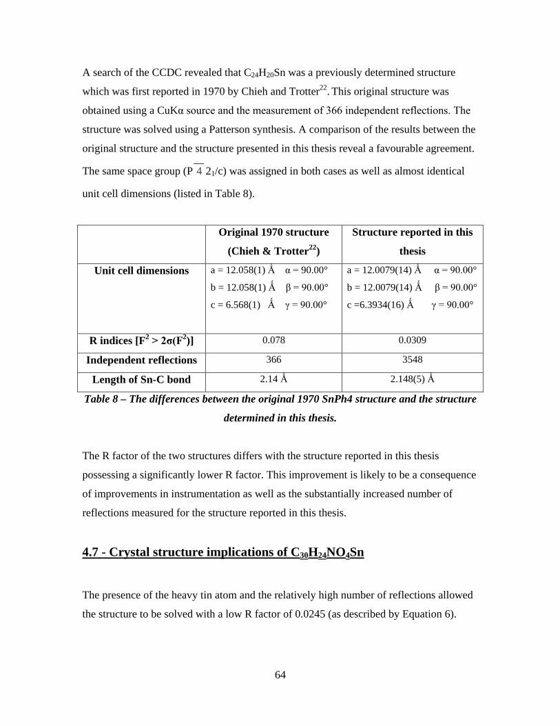
64

A search of the CCDC revealed that C24H20Sn was a previously determined structure

which was first reported in 1970 by Chieh and Trotter22. This original structure was

obtained using a CuKα source and the measurement of 366 independent reflections. The

structure was solved using a Patterson synthesis. A comparison of the results between the

original structure and the structure presented in this thesis reveal a favourable agreement.

The same space group (P 4 21/c) was assigned in both cases as well as almost identical

unit cell dimensions (listed in Table 8).

Original 1970 structure

(Chieh & Trotter22)

Structure reported in this

thesis

Unit cell dimensions a = 12.058(1) Ǻ α = 90.00°

b = 12.058(1) Ǻ β = 90.00°

c = 6.568(1) Ǻ γ = 90.00°

a = 12.0079(14) Ǻ α = 90.00°

b = 12.0079(14) Ǻ β = 90.00°

c =6.3934(16) Ǻ γ = 90.00°

R indices [F2 > 2σ(F2)] 0.078 0.0309

Independent reflections 366 3548

Length of Sn-C bond 2.14 Ǻ 2.148(5) Ǻ

Table 8 – The differences between the original 1970 SnPh4 structure and the structure

determined in this thesis.

The R factor of the two structures differs with the structure reported in this thesis

possessing a significantly lower R factor. This improvement is likely to be a consequence

of improvements in instrumentation as well as the substantially increased number of

reflections measured for the structure reported in this thesis.

4.7 - Crystal structure implications of C30H24NO4Sn

The presence of the heavy tin atom and the relatively high number of reflections allowed

the structure to be solved with a low R factor of 0.0245 (as described by Equation 6).

65

No classical hydrogen bonds were present in the crystal packing arrangement. It is likely

that the presence of an intramolecular hydrogen bond is not relevant to the crystal

packing arrangement.

Although the expected chemical structure and crystallographically three dimensional

structure are similar there are clear differences (Figure 4.12). The crystallographically

determined structure contains an extra two C-H units in addition to an extra carboxylate

unit. These differences imply that the attempted chemical synthesis was unsuccessful and

therefore requires modification if the desired product is to be obtained, and which has

been relayed to the synthetic chemist concerned.

Sn OO

H H ON

OCH3

Figure 4.12– The crystallographically determined structure has this chemical diagram

with the highlighted area corresponding to the deviation from the expected chemical

structure.

The monomer units are linked by a O-Sn bond measuring 2.6534(15) Ǻ. This is an

unusually long bond with regular tin to oxygen bonds expected to be around 2.10 Ǻ. A

search of the CCDC19 using CONQUEST20 software revealed 198 previously reported

structures contained a O-Sn bond of at least 2.65 Ǻ with bond lengths of up to 2.9 Ǻ

being reported. However none of these reported crystal structures possessed a significant

structural similarity to the structure of C30H24NO4Sn.

66

Part B – Macromolecular X-ray crystallography

67

Chapter 5

Macromolecular X-ray Crystallography

5.1 - Introduction

The principles of small molecule X-ray crystallography (as detailed in chapter one) are

equally applicable to the study of macromolecules such as proteins and viruses. However,

there are differences in procedure for the crystal structure determination and refinement.

The field of macromolecular X-ray crystallography is still relatively new with the first

protein crystal structures (those of myoglobin and haemoglobin) being solved in 1958 by

Kendrew and Perutz respectively. However thanks to advances in instrumentation as well

as technique development larger and more complex structures are now routinely studied.

Foremost amongst these developments is the advent of synchrotron radiation which

allows for the production of much more intense, well collimated and finely tuneable X-

rays. These properties are important as proteins consists of light, poorly scattering

elements primarily carbon, nitrogen and hydrogen as well as containing a high solvent

content. In addition methods of solving the phase problem specifically for use in

macromolecular crystallography have been developed.

Recently the 2009 Nobel Prize in chemistry was awarded to Ramakrishnan, Steitz and

Yonath for “Studies of the structure and function of the ribosome”23. This involved the

determination of a bacterial 70S ribosome consisting of two subunits with molecular

weights 800,000 and 1,500,000 using synchrotron X-ray crystallography. Obtaining high

resolution three dimensional structures of such macromolecules is important as it helps to

elucidate the mechanisms by which they operate.

A dedicated repository for the three dimensional structure of biological macromolecules

now exists24 and is free to access (available at www.pdb.org). As of 13/07/10 there were

66,324 structures deposited within the Protein Data Bank (PDB). The vast majority of

these being solved via X-ray crystallography (approx 57,000)

68

Although the number of structures solved by X-ray crystallography is growing annually

at an exponential rate problems are still prevalent. Foremost is the issue of growing

suitably sized diffraction grade single crystals. As the measured resolution is dependent

upon the crystal quality, well ordered crystals must be obtained if accurate structures are

to be obtained.

5.2.1 - Macromolecular crystallisation techniques

Small molecule crystallisation is a relatively simple process in comparison to

macromolecular crystallisation. This is because macromolecular crystallisation involves a

larger number of complicated interactions and is still poorly understood. Obtaining

diffraction grade, single crystals is a notorious ‘bottleneck’ and is often the rate limiting

step in the crystal structure determination. For example the pH at which crystallisation is

attempted will affect the net charge of a protein (via the protonation states of titratable

side chains). The resulting net charge will affect the solubility of the protein and therefore

the crystallisation process. A wide range of experimental conditions must be considered

and tailored, which may involve many attempts to perfect. The techniques used to induce

macromolecular crystallisation can be divided into four broad categories25. All four

methods involve different steps that crystal growth passes through26(Figure 5.1) such as

super saturation (which involves the formation of nuclei) and nucleation (which leads to

the formation of larger crystals.

Figure 5.1 – A phase diagram for crystal growth26.

69

5.2.2 – The batch method

This is the simplest method of crystallisation and is most useful when the conditions of

crystallisation have been narrowed down to a small range. A number of small glass vials

containing a protein and a precipitant (which is present at a level slightly less than at

which the protein precipitates) are prepared. The level of the protein and the precipitant is

varied between the vials therefore allowing the effect that the different concentrations

have on the crystallisation process to be observed. Usually, only microlitre volumes are

required. For example in the research behind this thesis crystallisations of 1ml and 2ml

were set up using this method.

5.2.3 - Dialysis

Dialysis uses a semi permeable membrane the pore sizes of which permit the passage of

solvent and small molecules. However as macromolecules are significantly larger they

are unable to pass through the pores. The macromolecule is slowly brought towards

supersaturation and its precipitation point by dialysis against a concentration of a

precipitating agent. It is also possible to induce crystallisation by altering the pH

(achieved by altering the concentration of the buffer). Like the batch method dialysis can

be performed on a bulk or a microlitre scale.

5.2.4 - Vapor diffusion methods

There are a number of variations of this method. Examples include the sitting drop,

hanging drop (Figure 1.11) and sandwich drop methods.

The basic idea behind them is that a small amount of the macromolecule is mixed with a

small amount of a precipitating agent. This drop is then allowed to equilibrate with a

reservoir of the precipitating agent contained within a closed system. An equilibrium will

form which will result in the water present in the sample diffusing out. Conversely the

concentration of the protein will increase, eventually reaching the supersaturation and

precipitation points.

70

5.2.5 - Hot box technique

This technique uses a temperature gradient to induce crystallisation. In this technique the

protein is dissolved at a low ionic strength in a test tube. The test tube is then suspended

in a thermos at high temperature (around 60°)27. The high temperature seeks to render the

protein more soluble and, as it slowly cools, a supersaturation point should be reached.

5.3.1 - Solving the phase problem in macromolecular crystallography

Owing to the increased complexity of proteins with respect to small molecules different

methods have been developed to solve the phase problem in macromolecular X-ray

crystallography.

A conventional Patterson synthesis cannot be performed as proteins often contain no

heavy atoms. In addition even small proteins contain a large number of atoms which

would lead to an uninterpretable Patterson map. For example lysozyme contains 2303

(non hydrogen) atoms, which would correspond to 5,303,809 vectors between the atoms!.

This results in far too many peaks for meaningful information to be extracted from the

Patterson map.

Direct methods are not applied to macromolecules as they require a relatively low

number of reflections for the computations to be effective. The large number of

reflections from a protein crystal would require an unrealistic amount of calculation to

retrieve the phases, for the computations to be effective.

As a result phase retrieval methods specific to macromolecular crystallography have been

developed, which are described below.

5.3.2 - Isomorphous replacement method

The isomorphous replacement method is based on the variation in intensities of the

diffraction spots belonging to two or more isomorphous crystals. Crystals can be

described as isomorphous if they have the same space group and almost identical unit cell

dimensions and atomic arrangements.

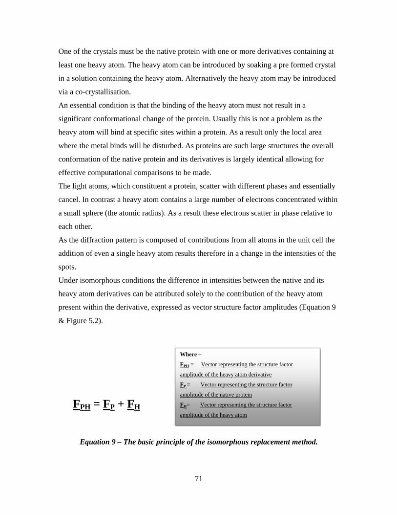
71

One of the crystals must be the native protein with one or more derivatives containing at

least one heavy atom. The heavy atom can be introduced by soaking a pre formed crystal

in a solution containing the heavy atom. Alternatively the heavy atom may be introduced

via a co-crystallisation.

An essential condition is that the binding of the heavy atom must not result in a

significant conformational change of the protein. Usually this is not a problem as the

heavy atom will bind at specific sites within a protein. As a result only the local area

where the metal binds will be disturbed. As proteins are such large structures the overall

conformation of the native protein and its derivatives is largely identical allowing for

effective computational comparisons to be made.

The light atoms, which constituent a protein, scatter with different phases and essentially

cancel. In contrast a heavy atom contains a large number of electrons concentrated within

a small sphere (the atomic radius). As a result these electrons scatter in phase relative to

each other.

As the diffraction pattern is composed of contributions from all atoms in the unit cell the

addition of even a single heavy atom results therefore in a change in the intensities of the

spots.

Under isomorphous conditions the difference in intensities between the native and its

heavy atom derivatives can be attributed solely to the contribution of the heavy atom

present within the derivative, expressed as vector structure factor amplitudes (Equation 9

& Figure 5.2).

FPH = FP + FH

Equation 9 – The basic principle of the isomorphous replacement method.

Where –

FPH = Vector representing the structure factor

amplitude of the heavy atom derivative

FP = Vector representing the structure factor

amplitude of the native protein

FH= Vector representing the structure factor

amplitude of the heavy atom

72

Figure 5.2 – A vectorial representation of the isomorphous replacement method

The differences in structure factor amplitudes can be used to calculate a difference

Patterson map which will consist of just the vectors between the heavy atoms. Combining

the difference map with the crystal symmetry should allow the heavy atom positions to be

determined. Once the heavy atom positions are known their contributions to the structure

factors can be determined.

The phase angles may be determined graphically by considering structure factors as

vectors. The vectors possess a length equal to the amplitude of the structure factor and a

direction corresponding to the estimated phase.

If only one derivative is considered and taking the assumption that FPH = FP + FH and that

FH can be calculated then there are two possible values that the phase may possess

If a second derivative is prepared there are again two possible values for the phase.

However only one value will be consistent with the first case thereby providing one

possible solution for the phase angle

A graphical representation of the phase angle calculation is known as a Harker

construction. The case when only one derivative is available will be considered first. In

this method a circle with a radius corresponding to the amplitude of the native protein

structure factor (FP) is drawn centred on the origin. A line corresponding to the position

and phase angle of the heavy atom (calculated from the difference Patterson map and

crystal symmetry) is then drawn. A second circle corresponding to this heavy atom

derivative is drawn (FPH) with the origin cantered on the end of the heavy atom line. The

FP

FPH

FH αH

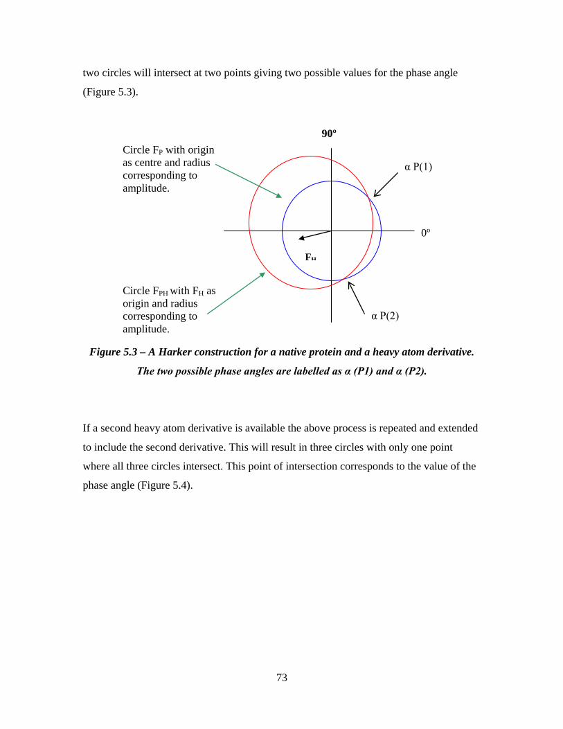
73

two circles will intersect at two points giving two possible values for the phase angle

(Figure 5.3).

Figure 5.3 – A Harker construction for a native protein and a heavy atom derivative.

The two possible phase angles are labelled as α (P1) and α (P2).

If a second heavy atom derivative is available the above process is repeated and extended

to include the second derivative. This will result in three circles with only one point

where all three circles intersect. This point of intersection corresponds to the value of the

phase angle (Figure 5.4).

α P(2)

α P(1) Circle FP with origin as centre and radius corresponding to amplitude.

Circle FPH with FH as origin and radius corresponding to amplitude.

FH

90º

0º

74

Figure 5.4 - A Harker construction for a native protein and two heavy atom derivatives.

The one possible phase angle is labelled as α (P1).

An inherent disadvantage of the method is the basically unavoidable introduction of some

level of errors through non-isomorphism. This is because crystals will never be

completely isomorphous. Therefore performing and comparing measurements of multiple

crystals will lead to the introduction of some level of errors. The effect of some errors

will progressively affect the higher resolution X-ray diffraction data and electron density

map details will become blurred.

5.3.3 - Anomalous scattering

Anomalous scattering is also dependent upon the presence of a heavy atom within a

protein. Conventional X-ray diffraction is a result of coherent scattering whereby the

incident X-rays cause electrons to vibrate. This effect generates radiation of a frequency

equal to the frequency of the incident radiation. However in the case of anomalous

scattering this is no longer true.

To enhance this effect the wavelength of the incident X-rays is tuned to correspond to an

absorption edge of a heavy atom present within the protein. An absorption edge involves

a small energy range and corresponds to an atomic transition, and which promotes the

α P(1) Circle (blue) FP with origin as centre and radius corresponding to amplitude.

Circle (red) FPH with FH as centre and radius corresponding to amplitude.

FH

90º

0º Circle (black) FPH2 with FH2 as centre and radius corresponding to amplitude.

FH2

75

heavy atom to an electronically excited state. This effect may involve the simple

promotion of a core electron to an unoccupied higher energy level or the complete

ejection of the electron from the atom (ionisation). This promotion or ejection of an

electron will alter the phase of the scattered radiation with respect to the scattering from

the light atoms. The effect of this phase change is equivalent to altering the path length of

the scattered radiation. This results in a change in intensities of the diffraction spots. The

increase in the anomalous scattering is coupled with a decrease in the coherent scattering.

This is because a proportion of the energy of the incident X-rays is used to create

transitions within the heavy atom.

An important use of anomalous scattering is in the determination of absolute

configurations. This can be achieved because anomalous scattering leads to a violation of

a condition known as Friedel`s law (which is assumed in what might be called

conventional X-ray crystallography). Friedel`s law states that a pair of symmetry related

reflections will have the same intensity and phases of equal magnitude but opposite in

sign (i.e. one will be positive the other negative). However at wavelengths close to an

absorption edge this condition is violated. This is because the heavy atoms will behave in

a different manner to the light atoms (in terms of how the phases are effected by the

scattering). This can be observed in the diffraction pattern as the intensities of the two

symmetry related spots being different e.g. F(hkl) will no longer equal F(-h,-k,-l).

The phases can be calculated graphically in the same way as in isomorphous replacement

using either a Harker construction or a vectorial representation (shown by Figures 5.2,

5.3, 5.4).

The expected structure factors for a pair of enantiomers can then be calculated and

compared with the observed structure factors which should then allow for assignment of a

specific enantiomer.

Anomalous scattering is now often the method of choice for solving the phase problem in

macromolecular X-ray crystallography. It is considered a more accurate method than

isomorphous replacement as it involves performing measurements on only one crystal as

opposed to two or three. This means that there are no errors introduced through non-

isomorphism. Isomorphous replacement can also be used in conjunction with anomalous

scattering resulting in an overall powerful method of phase determination.

76

5.3.4 - Molecular replacement28

The previous two methods of phase retrieval are required when the structure under study

is completely unknown. In contrast molecular replacement can be used when a suitably

related structure has been previously reported (known as the model). For example if a

model of oxyhaemoglobin is available it would assist in elucidating the structure of

deoxyhaemoglobin. As a rough guide a model can be considered suitable if the amino

acid sequence is greater than 30% identical to that of the structure under study. In the

case of oxyhaemoglobin and deoxyhaemoglobin this is obviously true (being 100%) but

for other examples it may be unclear as the success of the method is not guaranteed.

If this is the case the sequence identities may have to be determined.

If a suitable model is available then the phases from the model are used as initial

approximations for the phases of the structure under study. For this to be done the model

must firstly be correctly orientated and positioned in the unit cell of the structure under

study. This is done by systematically comparing predicted and observed structure factors

and thereby finding the orientation and position where there is an optimum correlation.

The orientation and positioning involves six positional parameters (three rotational angles

and three translational parameters). Performing calculations using all six parameters at

once presents an extremely large problem. This is because for N atoms in the asymmetric

unit there will be 6N parameters required to describe the solution. However Patterson

functions can be used, which allows the rotational and translational parameters to be

separated thereby simplifying the calculation convergence. Likelihood based methods

may also be used and are increasingly used in place of Patterson functions. These use

statistical methods in reciprocal space and can be divided into rotational and translational

functions in the same manner as for the Patterson methods.

As a result many molecular replacement programs choose a relatively small number of

good quality solutions provided by the rotational parameters and test these using the

translational parameters to finally provide a solution.

The rotational Patterson function involves calculating the Patterson map of the model and

rotating it over the observed Patterson map. The most probable orientation is found when

there is a close agreement between the two maps.

77

The translational Patterson function involves placing the centre of the model at all

positions in the unit cell of the structure under study. For each position attempted the

Patterson map can be calculated and compared to the observed Patterson map of the

structure under study. Where the two will agree yields the most likely position.

Once the correct orientation and position has been identified an electron density map of

the structure under study can be calculated. This electron density map is calculated using

the measured X-ray diffraction structure factor amplitudes from the structure under study,

and the estimated phases obtained form the model (that is correctly positioned and

orientated in the unit cell).

The difference map can be calculated, which will include areas of negative density

(corresponding to areas which are present in the model but do not fit the real density) and

areas of positive density (corresponding to areas which are not included in the model but

are present in the structure under study).

The molecular replacement method is increasingly popular as it is relatively quick to

perform. A high degree of automation is also involved with the rotation and translation

function computer programs now available. An example of a popular molecular

replacement computer program is PHASER.

5.4 – Rigid body and restrained refinement

Rigid body refinement is used as a first step in the refinement process for the

macromolecular adducts studied in this thesis. In rigid body refinement the distances

between the constituent atoms of a protein are fixed. In the simplest possible case this

means that the entire protein is treated as one large, rigid molecule. Alternatively the

protein may be divided into a small number of subunits (e.g. beta sheets or alpha helices).

The rigid blocks of the structure are then placed to match the experimentally determined

electron density.

In restrained refinement the bond lengths and angles of the protein are allowed a certain

degree of freedom. This means that the bond lengths and angles are allowed to vary

within a small range but not but a large amount i.e. they are restrained to within a certain

range. Although bond lengths and angles are perhaps the most important restraint used, a

78

large number of other restraints are possible (such as forcing peptide bonds to adopt a

planar conformation).

The aim is the same as small molecule refinement refinement, which is the optimal

correlation between the observed and calculated structure factor amplitudes.

5.5 - The R free factor

In addition to the conventional R factor detailed in Chapter one macromolecular

crystallography uses another criterion to describe the correctness of a structure. The

additional criterion is known as the R free factor and is calculated using the same

equation as the conventional R factor (Equation 6). However the R free factor is instead

calculated exclusively from a small percentage of reflections (typically around 5%) which

are excluded from the refinement process. This avoids using the same data to perform

refinement as well as measuring the correctness of the structure.

The R free factor is normally higher than the conventional R factor although both should

possess values relatively close together. A difference of up to 6% is usually tolerated.

In addition to monitoring the progress of the model refinement the R free factor is used to

validate that the conventional R factor is not being artificially lowered by the addition of

an increased number of parameters.

79

Chapter 6

Crystal structure determination and model refinement of a co-

crystallisation of HEWL and TA6Br12

6.1.1 - Introduction

This chapter details the data collection procedure and subsequent model refinement of a

co-crystallisation of hen egg white lysozyme (HEWL) and Ta6Br12. The motivation for

conducting this work lies in facilitating technique development. It is hoped that the

crystal structure determination will lead to a well resolved structure which is solved to a

satisfactory resolution. This model structure can then be compared to models obtained

using data gathered from newly developed methods. Ideally this will allow for the

accuracy of methods to be accessed and weaknesses identified and improved upon. The

advent of the free electron laser has catalysed technique development in a number of

areas. These include protein powder diffraction and the possibility of using nanoclusters

or even single molecules as opposed to crystals. Developments such as these which

remove the need for crystals (which are often difficult or sometimes impossible to obtain)

could yield new possibilities.

6.1.2 - Introduction to lysozyme

Lysozyme is an enzyme that catalyses the cleaving of polysaccharide chains present in

the cell walls of bacteria29, 30. This has the effect of causing the cell wall to rupture.

Without the rigidity supplied by the cell wall the bacteria burst as a result of intolerable

osmotic pressure. As a result of this antibacterial function lysozyme is often termed as a

natural antibiotic. It is commonly found in tears, saliva and in hen egg white (the form

used in this thesis).

Lysozyme is a commonly used test enzyme within crystallography for a variety of

reasons. It is cheap and easy to obtain. Its structure has been previously well studied

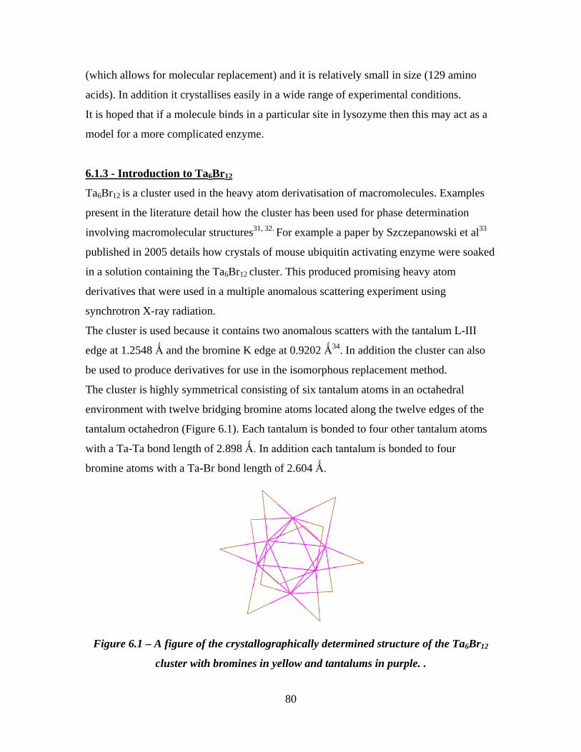
80

(which allows for molecular replacement) and it is relatively small in size (129 amino

acids). In addition it crystallises easily in a wide range of experimental conditions.

It is hoped that if a molecule binds in a particular site in lysozyme then this may act as a

model for a more complicated enzyme.

6.1.3 - Introduction to Ta6Br12

Ta6Br12 is a cluster used in the heavy atom derivatisation of macromolecules. Examples

present in the literature detail how the cluster has been used for phase determination

involving macromolecular structures31, 32. For example a paper by Szczepanowski et al33

published in 2005 details how crystals of mouse ubiquitin activating enzyme were soaked

in a solution containing the Ta6Br12 cluster. This produced promising heavy atom

derivatives that were used in a multiple anomalous scattering experiment using

synchrotron X-ray radiation.

The cluster is used because it contains two anomalous scatters with the tantalum L-ІІІ

edge at 1.2548 Ǻ and the bromine K edge at 0.9202 Ǻ34. In addition the cluster can also

be used to produce derivatives for use in the isomorphous replacement method.

The cluster is highly symmetrical consisting of six tantalum atoms in an octahedral

environment with twelve bridging bromine atoms located along the twelve edges of the

tantalum octahedron (Figure 6.1). Each tantalum is bonded to four other tantalum atoms

with a Ta-Ta bond length of 2.898 Ǻ. In addition each tantalum is bonded to four

bromine atoms with a Ta-Br bond length of 2.604 Ǻ.

Figure 6.1 – A figure of the crystallographically determined structure of the Ta6Br12

cluster with bromines in yellow and tantalums in purple. .

81

The Ta6Br12 was supplied by Jena Bioscience in the form of a fine green powder.

The cluster has a +2 charge which is countered by two bromine ions in the preparation

supplied. It is a possibility that the positive charge on the cluster will cause it to bind to

side chains in the protein which possess negative charges (a Coulombic interaction).

The binding of Ta6Br12 to lysozyme was first investigated using single crystal X-ray

crystallography by Corey et al in 196235. However due to the technological restrictions of

the time no three dimensional structure was produced. It is hoped that the subsequently

vast improvements in instrumentation and technique development will enable the three

dimensional structure to be determined.

6.2 – Co-crystallisation procedure of HEWL and Ta6Br12

The crystals of hen egg white lysozyme and Ta6Br12 were grown using a batch method

co-crystallisation (adopted from Blundell and Johnson25).

A sodium acetate buffer was used to regulate the pH. This was prepared by dissolving

0.54g of sodium acetate trihydrate (CH3COONa.3H2O) in 50ml of distilled water in a

volumetric flask. Once all solids had dissolved 229µl of acetic acid (CH3COOH) was

added to the solution which was then stirred for five minutes. The volume of the solution

was then accurately increased to 100ml. The resulting solution was pH 4.7 with an

acetate concentration of 0.04M.

The precipitating agent used was a 10% salt solution. This was prepared by adding 10g

of salt (NaCl) to a volumetric flask. Distilled water was then added to accurately bring

the volume to 100ml.

For the co-crystallisation 0.04M acetate buffer (1ml) was added to lysozyme (50mg) in a

small glass vial. The solution was stirred for 5 minutes to ensure the lysozyme powder

had fully dissolved. At this point one aliquot (1mg) of Ta6Br12 was added. Stirring the

solution for five minutes with the end of a Finn pipette was essential to ensure the Ta6Br12

had fully dissolved. The solution was now pale green in colour. Finally, 10% salt solution

(1ml ) was added over a five minute period to help induce crystallisation. The final

82

solution was stirred for five minutes. The vial was then left in an undisturbed position at

room temperature.

After three days it was found that a large number of single crystals were present on the

bottom of the vial. The crystals appeared to be of good quality with no visible defects. In

addition the crystals extinguished well under crossed polarisers. The crystals were green

in colour, like Ta6Br12 (Figure 6.2).

Figure 6.2 – A picture of the Ta6Br12 & HEWL crystals as viewed under a microscope

after 3 days. Crystals were approximately 0.1mm in length at this point in time.

6.3 – X-ray diffraction data collection procedure

Glycerol (4µl) was used as a cryoprotectant and was added to mother liquor (12µl) which

contained the crystals. A low level of glycerol (25%) was required as it appeared to

slowly interact with the crystals. From this a single, green crystal measuring 0.2mm

across was selected. The crystal was fitted onto a fibre mesh and then mounted onto an R-

Axis imaging plate diffractometer with a rotating copper anode source.

The detector to crystal distance was carefully considered. This is because moving the

detector further away from the crystal will reduce the amount of incoherent scattering

from the crystal and thus improve the accuracy of the data. However moving the detector

further away will also result in a smaller range of θ angles being recorded which will

83

cause a reduction in the measured resolution. In this case the crystal to detector distance

was set at 120mm and the data collection temperature at 100K.

A full 360º of data were collected with an exposure time of seven minutes per degree.

Figure 6.3 is one of the X-ray diffraction images obtained. A summary of the data

collection statics is listed in Table 9.

Figure 6.3 – An X-ray diffraction pattern image from the Ta6Br12 & HEWL data

collection.

The resulting data was processed, merged and scaled using the d*trek program36 (part of

the Rigaku suite of programs). It was decided to remove the images in the ranges 1-74º

and 342 - 360º from the processing as removing these images improved the value of

Rmerge. An initial model structure was obtained using the model replacement method.

This was done using the PHASER computer program which is part of the CCP4i suite37.

The resolution of the model was solved to 1.95Ȧ.

84


Space group P 43 21 2

Unit cell dimensions a = 78.9964 Ǻ α = 90.00°

b = 78.9964 Ǻ β = 90.00°

c = 36.8507 Ǻ γ = 90.00°

Unit cell volume 229964 Ǻ3

Data collection temperature 100 K

Radiation CuKα rotating anode

Diffractometer R-Axis

Detector Image plate

Crystal size 0.20 x 0.20mm

Crystal mosaicity 1.434°



Data completeness 100% (100%)

<I σI> 13.2 (3.8)

Average redundancy 10.49 (10.44)

Rmerge 0.085 (0.433)

Resolution range 55.86 - 1.95 (2.02 - 1.95)

Table 9 – The summary of the X-ray diffraction data collection of HEWL and Ta6Br12

crystal. Values in parentheses indicate the last resolution shell

6.4 – Model refinement procedure The following steps were performed to move from an initial model to a final structure.

All the refinement steps were performed in the refmac5 program which is part of the

CCP4i suite. Map inspection and model building was performed in the COOT38 program.

Step 1

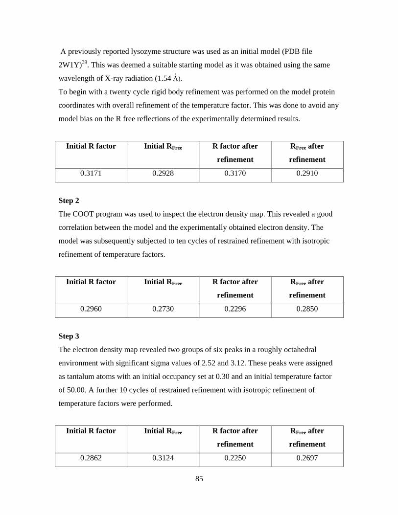
85

A previously reported lysozyme structure was used as an initial model (PDB file

2W1Y)39. This was deemed a suitable starting model as it was obtained using the same

wavelength of X-ray radiation (1.54 Ǻ).

To begin with a twenty cycle rigid body refinement was performed on the model protein

coordinates with overall refinement of the temperature factor. This was done to avoid any

model bias on the R free reflections of the experimentally determined results.

Initial R factor Initial RFree R factor after

refinement

RFree after

refinement

0.3171 0.2928 0.3170 0.2910

Step 2

The COOT program was used to inspect the electron density map. This revealed a good

correlation between the model and the experimentally obtained electron density. The

model was subsequently subjected to ten cycles of restrained refinement with isotropic

refinement of temperature factors.


refinement

RFree after

refinement

0.2960 0.2730 0.2296 0.2850

Step 3

The electron density map revealed two groups of six peaks in a roughly octahedral

environment with significant sigma values of 2.52 and 3.12. These peaks were assigned

as tantalum atoms with an initial occupancy set at 0.30 and an initial temperature factor

of 50.00. A further 10 cycles of restrained refinement with isotropic refinement of

temperature factors were performed.


refinement

RFree after

refinement

0.2862 0.3124 0.2250 0.2697

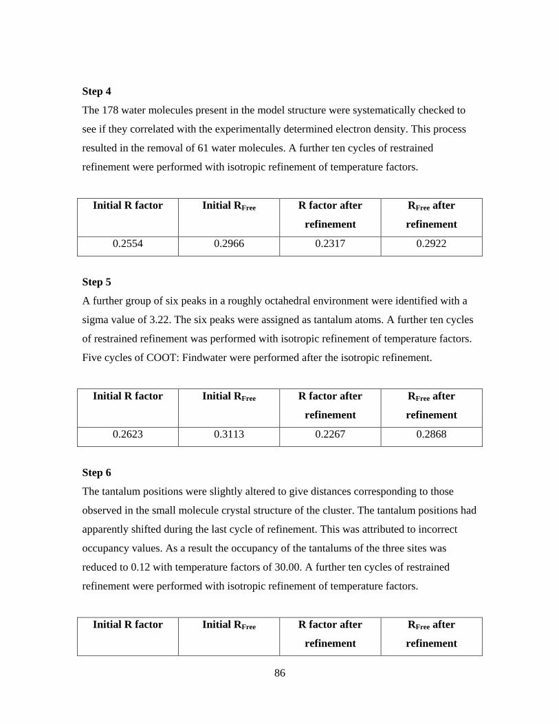
86

Step 4

The 178 water molecules present in the model structure were systematically checked to

see if they correlated with the experimentally determined electron density. This process

resulted in the removal of 61 water molecules. A further ten cycles of restrained

refinement were performed with isotropic refinement of temperature factors.


refinement

RFree after

refinement

0.2554 0.2966 0.2317 0.2922

Step 5

A further group of six peaks in a roughly octahedral environment were identified with a

sigma value of 3.22. The six peaks were assigned as tantalum atoms. A further ten cycles

of restrained refinement was performed with isotropic refinement of temperature factors.

Five cycles of COOT: Findwater were performed after the isotropic refinement.


refinement

RFree after

refinement

0.2623 0.3113 0.2267 0.2868

Step 6

The tantalum positions were slightly altered to give distances corresponding to those

observed in the small molecule crystal structure of the cluster. The tantalum positions had

apparently shifted during the last cycle of refinement. This was attributed to incorrect

occupancy values. As a result the occupancy of the tantalums of the three sites was

reduced to 0.12 with temperature factors of 30.00. A further ten cycles of restrained

refinement were performed with isotropic refinement of temperature factors.


refinement

RFree after

refinement

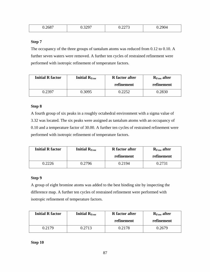
87

0.2687 0.3297 0.2273 0.2904

Step 7

The occupancy of the three groups of tantalum atoms was reduced from 0.12 to 0.10. A

further seven waters were removed. A further ten cycles of restrained refinement were

performed with isotropic refinement of temperature factors.


refinement

RFree after

refinement

0.2397 0.3095 0.2252 0.2830

Step 8

A fourth group of six peaks in a roughly octahedral environment with a sigma value of

3.32 was located. The six peaks were assigned as tantalum atoms with an occupancy of

0.10 and a temperature factor of 30.00. A further ten cycles of restrained refinement were

performed with isotropic refinement of temperature factors.


refinement

RFree after

refinement

0.2226 0.2796 0.2194 0.2731

Step 9

A group of eight bromine atoms was added to the best binding site by inspecting the

difference map. A further ten cycles of restrained refinement were performed with

isotropic refinement of temperature factors.


refinement

RFree after

refinement

0.2179 0.2713 0.2178 0.2679

Step 10

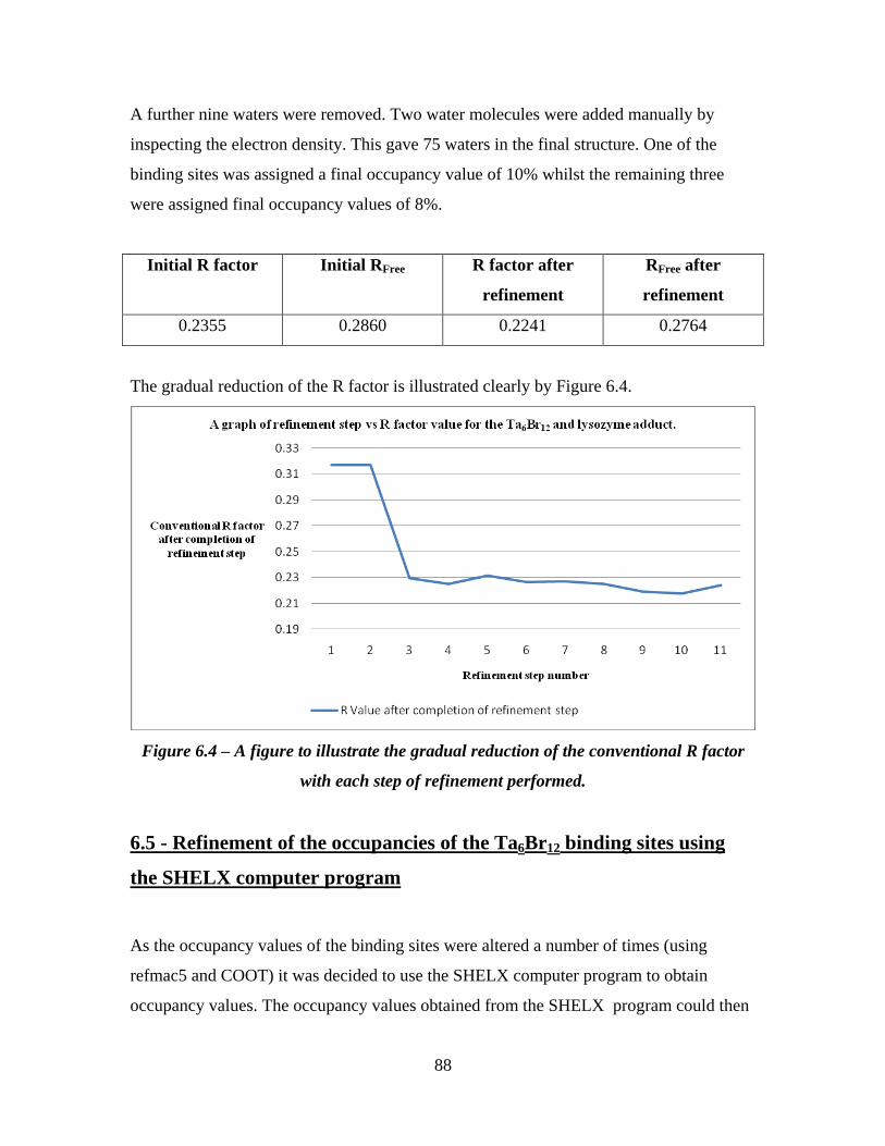
88

A further nine waters were removed. Two water molecules were added manually by

inspecting the electron density. This gave 75 waters in the final structure. One of the

binding sites was assigned a final occupancy value of 10% whilst the remaining three

were assigned final occupancy values of 8%.


refinement

RFree after

refinement

0.2355 0.2860 0.2241 0.2764

The gradual reduction of the R factor is illustrated clearly by Figure 6.4.

Figure 6.4 – A figure to illustrate the gradual reduction of the conventional R factor

with each step of refinement performed.

6.5 - Refinement of the occupancies of the Ta6Br12 binding sites using

the SHELX computer program

As the occupancy values of the binding sites were altered a number of times (using

refmac5 and COOT) it was decided to use the SHELX computer program to obtain

occupancy values. The occupancy values obtained from the SHELX program could then

89

be compared to the occupancy values already being used. It was hoped that this may

provide an indication of the accuracy of the values being used.

The SHELX program required a model structure (known as a fragment). This was

provided in the form of a crystallographically determined structure40 of Ta6Br12.6H2O

from the ICSD database. This structure contained the ideal bond lengths present within

the molecule as well as accurate unit cell dimensions. The coordinated waters molecules

were removed from this cluster as they were not present in the form of the cluster which

is bound to lysozyme. The idea cluster was then fixed one at a time into the four binding

sites within lysozyme. These locations had been determined by inspecting the electron

density map using the COOT computer program. Although all six of the tantalum atoms

in the four binding sites had been located using COOT the bromine atoms had not.

Therefore the bromine atom positions were approximated using the position of a tantalum

atom to which a particular bromine was attached to.

After one Ta6Br12 cluster had been fixed into place, ten cycles of refinement were

performed in the SHELX computer program. After the refinement another Ta6Br12 cluster

was fixed followed by 10 cycles of refinement and so on. After each cycle of refinement

the resulting R factor and occupancy values were recorded.

The SHELX computer program calculates theoretical electron density from the ideal

cluster and attempts to match it and the unit cell dimensions to the experimentally

determined electron density. It refines the position of the cluster and its occupancy value

based on the minimisation of the difference between the observed and calculated electron

density.

After one Ta6Br12 fragment has been placed into a binding site.

R factor Occupancy of binding site

24.61 9.9%

After two Ta6Br12 fragments have been placed into binding sites.

R factor Occupancy of binding site 1 Occupancy of binding site 2

0.2446 8.7% 8.2%

90

After three Ta6Br12 fragments have been placed into binding sites

R factor Occupancy of binding site 1 Occupancy of binding

site 2

Occupancy of binding

site 3

0.2439 9.4% 10.7% 10.2%

After four Ta6Br12 fragments have been placed into binding sites

R factor Occupancy of

binding site 1

Occupancy of

binding site 2

Occupancy of

binding site 3

Occupancy of

binding site 4

0.2431 9.2% 10.0% 10.0% 10.0%

After all four Ta6Br12 clusters had been placed, ten cycles of refinement were carried out

which yielded the results above. However the refinement process did not converge

satisfactorily. As a result the number of refinement cycles was increased from ten to

thirty in the hope of obtaining more accurate results. Convergence was achieved once the

number of cycles was increased, the results of which should be more accurate than

previous results.

After four Ta6Br12 fragments have been placed into binding sites. (30 cycle

refinement)

R factor Occupancy of

binding site 1

Occupancy of

binding site 2

Occupancy of

binding site 3

Occupancy of

binding site 4

0.2318 10.1% 12.4% 9.6% 16.4%

The values of 10.1% and 9.6% are relatively similar to those obtained using the refmac5

and COOT computer programs. However the values of 12.4% and 16.4% are

significantly larger. Inspection of the .res file obtained from SHELX revealed that the

clusters in these positions had been placed too close to the protein. It is possible that this

may account for the high occupancy values observed.

The evolution of the occupancies of each of the four binding sites with each step of

refinement is clearly illustrated in a graphically format by Figure 6.5.

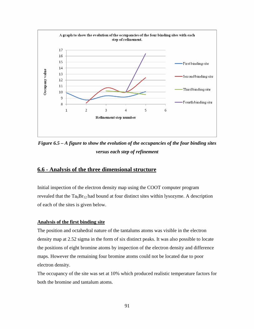
91

Figure 6.5 – A figure to show the evolution of the occupancies of the four binding sites

versus each step of refinement

6.6 - Analysis of the three dimensional structure

Initial inspection of the electron density map using the COOT computer program

revealed that the Ta6Br12 had bound at four distinct sites within lysozyme. A description

of each of the sites is given below.

Analysis of the first binding site

The position and octahedral nature of the tantalums atoms was visible in the electron

density map at 2.52 sigma in the form of six distinct peaks. It was also possible to locate

the positions of eight bromine atoms by inspection of the electron density and difference

maps. However the remaining four bromine atoms could not be located due to poor

electron density.

The occupancy of the site was set at 10% which produced realistic temperature factors for

both the bromine and tantalum atoms.

92

Figure 6.6 – The electron density surrounding the first Ta6Br12 to lysozyme binding

site.

The tantalum atoms are arranged in a fairly regular octahedral environment with the

equatorial tantalums joined by bonds with distances of 2.49 Ǻ , 2.30 Ǻ, 3.11 Ǻ and 3.36

Ǻ. The two axial tantalums are separated by 4.47 Ǻ. These distances compare favourably

with the actual values40 of .2.901(7) Ǻ and 4.096(10) Ǻ respectively.

Figure 6.7 – A figure to show the distances between the tantalum atoms in the first

binding site. Also shown are the distances to the nearest residues.

93

There are two possible residues with which the cluster may interact (as shown in Figure

6.7). The closest residue is arginine 125, the amine groups of which are 1.95 Ǻ and 3.24

Ǻ away from the closest tantalum atoms. It is likely that at the crystallisation pH of 4.7,

arginine would be protonated which would generate a positive charge. As the cluster is

also positively charged it is surprising to find the two so close together.

The next nearest residue is aspartic acid 119 which is 2.67 Ǻ away. It is likely that at the

crystallisation pH of 4.7 aspartic acid would possess a negative charge. As a result it is a

possible that there is a columbic interaction between the cluster and this residue.

The third nearest amino acid is glutamine 121 which is 4.12 Ǻ away which appears to be

too great a distance for an interaction to occur.

Analysis of the second binding site

The position and octahedral environment of the six tantalum atoms was clearly visible at

3.12 sigma. However the position of the bromine atoms could not be determined due to

poor electron density .The tantalum atoms are arranged in a poor octahedral environment

with the equatorial tantalum atoms joined by bonds with distances of 2.70 Ǻ, 3.80 Ǻ, 3.52

Ǻ and 2.09 Ǻ. The two axial tantalum atoms are separated by a distance of 5.54 Ǻ. These

distances display substantial deviation from the ideal values. In addition it was found that

the tantalum positions appeared to shift significantly with each cycle of refinement. This

is probably due to the low occupancy of the binding site, which was set at 8%. The

temperature factors of the bromine atoms were consistent with those of the previous site.

94

Figure 6.8 – The electron density surrounding the second Ta6Br12 to lysozyme binding

site.

The site is most closely located to a carbon atom of a proline residue which is 2.92 Ǻ

away. As the carbon will possess no charge at the crystallisation pH (pH = 4.7) it is

unclear how the cluster interacts at this particular location.

Figure 6.9 – A figure to show the distances between the tantalum atoms in the second

binding site. Also shown is the distance to the nearest residue.

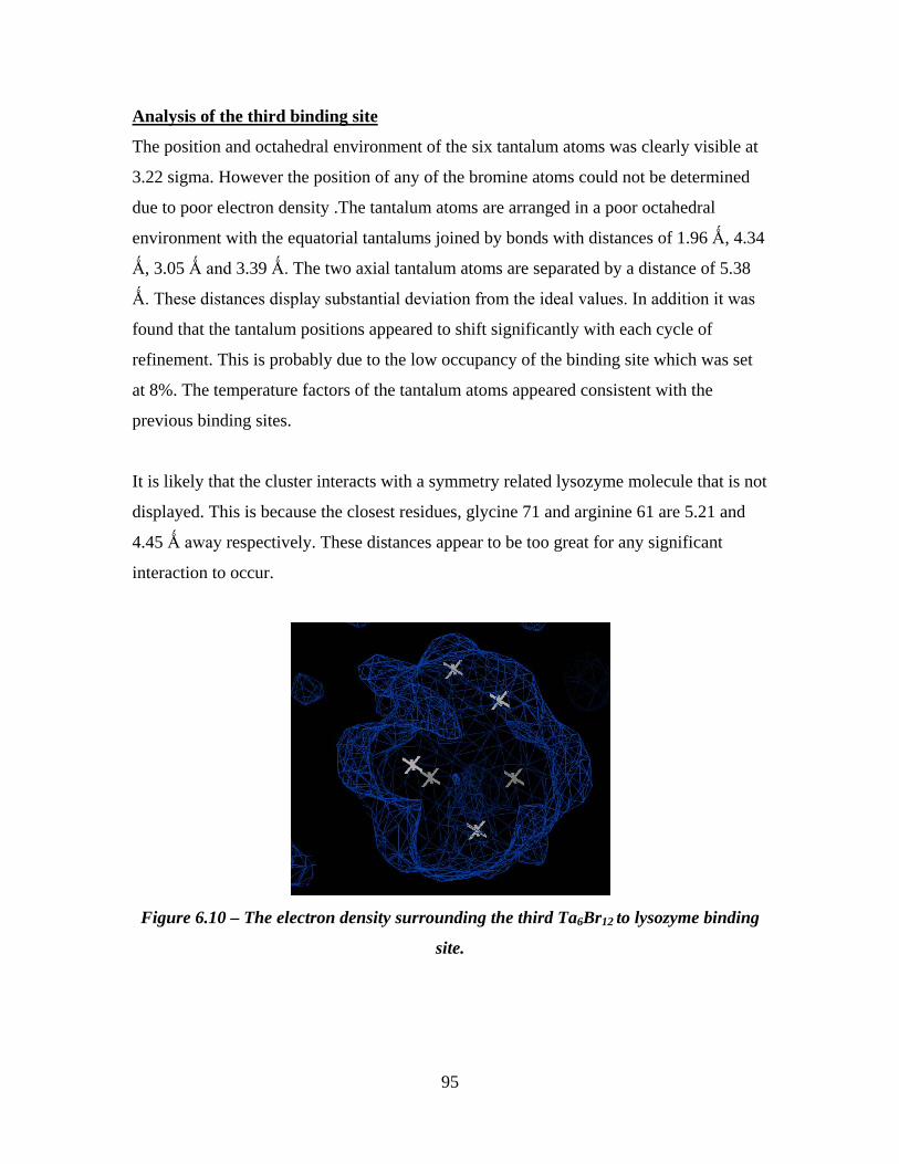
95

Analysis of the third binding site


3.22 sigma. However the position of any of the bromine atoms could not be determined

due to poor electron density .The tantalum atoms are arranged in a poor octahedral

environment with the equatorial tantalums joined by bonds with distances of 1.96 Ǻ, 4.34

Ǻ, 3.05 Ǻ and 3.39 Ǻ. The two axial tantalum atoms are separated by a distance of 5.38

Ǻ. These distances display substantial deviation from the ideal values. In addition it was

found that the tantalum positions appeared to shift significantly with each cycle of

refinement. This is probably due to the low occupancy of the binding site which was set

at 8%. The temperature factors of the tantalum atoms appeared consistent with the

previous binding sites.

It is likely that the cluster interacts with a symmetry related lysozyme molecule that is not

displayed. This is because the closest residues, glycine 71 and arginine 61 are 5.21 and

4.45 Ǻ away respectively. These distances appear to be too great for any significant

interaction to occur.

Figure 6.10 – The electron density surrounding the third Ta6Br12 to lysozyme binding

site.

96

Figure 6.11 – A figure to show the distances between the tantalum atoms in the third


Analysis of the fourth binding site


3.32 sigma. However the position of any of the bromine atoms could not be determined

due to poor electron density. The tantalum atoms are arranged in a poor octahedral

environment with the equatorial tantalum atoms joined by bonds of distances 4.60 Ǻ,

3.11 Ǻ, 3.38 Ǻ and 3.88 Ǻ. The two axial tantalum atoms are separated by a distance of

5.07 Ǻ. The tantalum atoms appeared to shift during the refinement process probably due

to the low occupancy of the site which was set at 8%. The temperature factors of the

tantalum atoms appeared consistent with the previous binding sites.

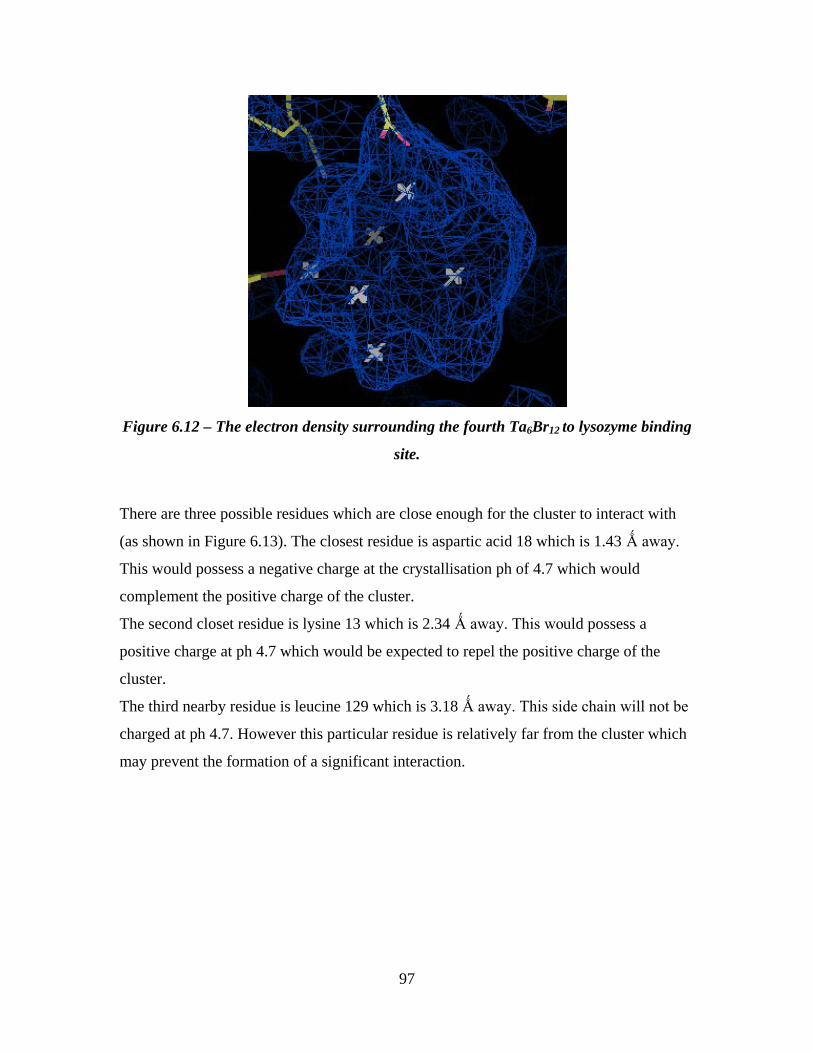
97

Figure 6.12 – The electron density surrounding the fourth Ta6Br12 to lysozyme binding

site.

There are three possible residues which are close enough for the cluster to interact with

(as shown in Figure 6.13). The closest residue is aspartic acid 18 which is 1.43 Ǻ away.

This would possess a negative charge at the crystallisation ph of 4.7 which would

complement the positive charge of the cluster.

The second closet residue is lysine 13 which is 2.34 Ǻ away. This would possess a

positive charge at ph 4.7 which would be expected to repel the positive charge of the

cluster.

The third nearby residue is leucine 129 which is 3.18 Ǻ away. This side chain will not be

charged at ph 4.7. However this particular residue is relatively far from the cluster which

may prevent the formation of a significant interaction.

98

Figure 6.13 – A figure to show the distances between the tantalum atoms in the fourth


6.7 - Implications of the three dimensional structure

Four Ta6Br12 binding sites to lysozyme were clearly identified at 1.95 Ȧ. The tantalum

atoms present in all four binding sites were located with bond angles and positions

roughly corresponding to those of an octahedral environment. It was possible to locate

eight bromine atoms in only one of the binding sites. The occupancy of one of the

binding sites was around 10% with the remaining three binding sites around 8%.

The high amount of electron density present within the Ta6Br12 cluster allows for it to be

easily located using the electron density map, even at the low occupancies reported here.

In contrast to this the binding of another bromine containing, transition metal cluster,

K2PtBr6 to HEWL has been previously reported41. The cluster was introduced using a

soaking method which resulted in largest occupancies of around 50% for the longest soak

time used of 170 minutes. For the shorter time used of ten minutes this occupancy was

33%. Future work on this cluster may include focusing on its potential susceptibility to

radiation damage with possible loss of the bromine atoms.

The three dimensional structure obtained should provide a model to allow for comparison

with models obtained using new methodologies such a s protein powder X-ray diffraction

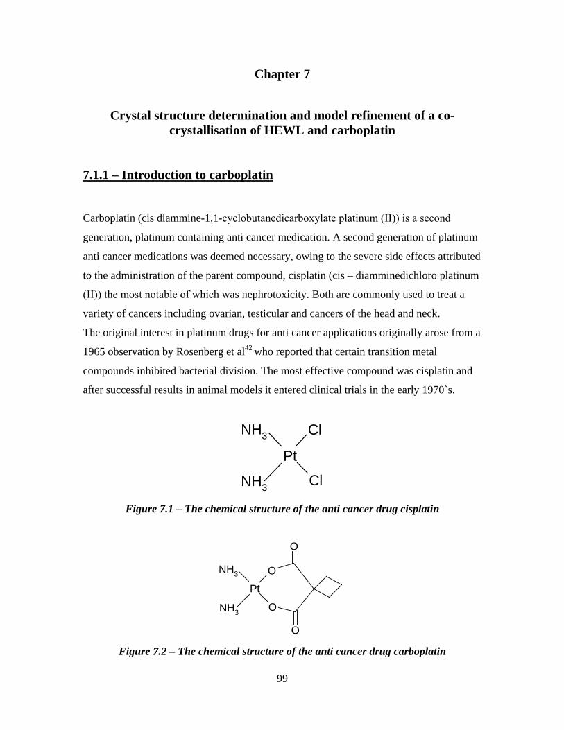
99

Chapter 7

Crystal structure determination and model refinement of a co-crystallisation of HEWL and carboplatin

7.1.1 – Introduction to carboplatin

Carboplatin (cis diammine-1,1-cyclobutanedicarboxylate platinum (ΙΙ)) is a second

generation, platinum containing anti cancer medication. A second generation of platinum

anti cancer medications was deemed necessary, owing to the severe side effects attributed

to the administration of the parent compound, cisplatin (cis – diamminedichloro platinum

(ΙΙ)) the most notable of which was nephrotoxicity. Both are commonly used to treat a

variety of cancers including ovarian, testicular and cancers of the head and neck.

The original interest in platinum drugs for anti cancer applications originally arose from a

1965 observation by Rosenberg et al42 who reported that certain transition metal

compounds inhibited bacterial division. The most effective compound was cisplatin and

after successful results in animal models it entered clinical trials in the early 1970`s.

Pt

NH3

NH3

Cl

Cl

Figure 7.1 – The chemical structure of the anti cancer drug cisplatin

Pt

NH3

NH3

O

O

O

O Figure 7.2 – The chemical structure of the anti cancer drug carboplatin

100

The cis isomers of both compounds are used for therapeutic applications as the trans

isomers display no biological activity. Cisplatin contains two labile cis chloride ions

which act as leaving groups. This is in addition to two relatively stable ammonia groups

which in conjugation with the chloride ions are arranged in a square planar geometry

(Figure 7.1).

In contrast carboplatin contains a more stable bidentate dicarboxylate ligand in place of

the chloride ions in addition to the two ammonia groups (Figure 7.2).

It is widely accepted that the labile chlorine ions of cisplatin are exchanged for

nucleophilic groups which result in the formation of chemically stable links.

The administered form of carboplatin reacts with water to form an active hydrated

intermediate. This intermediate is only formed inside cells as the chloride ion

concentration outside cells is sufficiently high enough to prevent hydrolysis. However,

inside cells the chloride ion concentration is low enough for hydrolysis to take place. This

results in the displacement of one chloride ion by a water molecule. The water molecule

is subsequently displaced which allows the platinum atom to coordinate with

nucleophiles present within the DNA helix. The displacement of the second chloride ion

allows the formation of interstrand cross links43.

Cisplatin displays little affinity for the sugars and phosphates but instead reacts with the

purine and pyridimine base pairs of DNA. The primary target of cisplatin at physiological

pH is the N7 atoms of guanine and adenine. The reaction most commonly results in

intrastrand cross linking of two neighbouring guanines which accounts for the majority of

the cross linking seen (around 60%). The cross linking caused by cisplatin causes a major

bending of the DNA helix towards the major groove of DNA44. It is possible that this

structural change is sufficient to inhibit further DNA synthesis resulting in cell death. The

crystal structure of cisplatin and duplex DNA has been determined at 2.6 Ǻ resolution by

Takahara et al45. The structure was solved using the multiple isomorphous derivative

method. This crystal structure support the formation of guanine-guanine cross links

within the DNA.

Carboplatin appears to act via a similar mechanism owing to the more stable nature of the

bidentate carboxylate ligand it acts at a slower rate. In addition for carboplatin the drug

101

passing through the kidneys is not aquated. Therefore it does not react with the kidney

tissue which is the cause of the nephrotoxicity displayed by cisplatin.

7.1.2 – Introduction to work by Casini et al (2006)

The interest in carboplatin originally arose from a paper by Casini et al46 which was

published in 2006. In this paper the authors studied the adducts of anticancer platinum

drugs with hen egg-white lysozyme (HEWL) using both electron spray ionisation mass

spectrometry (ESI-MS) and single crystal X-ray crystallography. The results obtained

using ESI-MS indicated that the protein platination had only partially taken place. This

result was confirmed using ICP-OES (inductively coupled optical emission spectroscopy)

which indicated that platination levels were around 50% for cisplatin and less than 15%

for carboplatin. This proved that the cisplatin and carboplatin had bound to HEWL albeit

at seemingly low binding occupancies.

It was surprising that the platination was of such low levels as high excesses of the

anticancer drugs were used (three fold excess of anticancer drug with respect to

lysozyme) in addition to long soaking times.

In order to gain a more precise idea of the adduct structures and the location of the metal

binding sites single crystal X-ray crystallography was employed. Two sets of lysozyme

crystals were grown using the hanging drop method and separately soaked in solutions

containing excesses of carboplatin and cisplatin. It was found that diffraction quality

crystals were only obtained in the case of cisplatin. The adduct was subsequently solved

at a resolution of 1.9Ǻ.

7.1.3 – Previous work by the Helliwell group

As the soaking method had previously proved to be unsuccessful it was decided by us to

pursue a co-crystallisation of HEWL and carboplatin. The initial attempt was performed

by Joanne Meredith for a MChem dissertation47. For the crystallisation hen egg white

lysozyme (49mg) was transferred to a glass vial to which a 0.04m acetate buffer solution

(1ml) was also added (preparation as described in Chapter. The mixture was gently

stirred for five minutes to ensure the lysozyme powder had fully dissolved. Once

completed carboplatin (3.713mg, 5mM) was added followed by a further five minutes of

102

gentle stirring. Finally 10% salt solution (1ml) was added gradually over a period of five

minutes after which the solution was stirred for a further five minutes. At this point the

glass vial was sealed and left undisturbed at room temperature. The amounts of

carboplatin and lysozyme were chosen to give a three fold excess of carboplatin with

respect to lysozyme (in terms of moles).

After inspection after 72 hours a larger number of colourless block like crystals with a

typical size of 0.3-0.35mm were present. Unfortunately after data collection and

processing it was discovered that the occupancy of the carboplatin was low. There was

insufficient electron density to provide a satisfactory structure so it was decided to find a

method to improve the occupancy. However from this initial wok it appeared that

carboplatin bound to the sugar binding, active site of lysozyme. This was a promising

result as it may indicate the possibility of using carboplatin as an inhibitor of sugar

binding enzymes.

7.2 – Co-crystallisation method and optimisation of the conditions

Following on from the work carried out by Joanne Meredith it was decided to attempt use

a chemical additive to attempt to improve the occupancy of the carboplatin binding. A

search of literature sources indicated that both lysozyme and carboplatin are soluble in

dimethyl sulfoxide (DMSO)48,49. It was envisaged that if the solubility of both

components is increased then the occupancy of the carboplatin binding will also increase.

In addition it was decided to increase the carboplatin concentration to 10mM in the hope

this would promote increased binding.

A paper by Lu et al50 published in 2002 describes the growth of lysozyme crystals from a

binary mixture consisting of 12.5% DMSO and water. It was therefore decided to attempt

to recreate these conditions with the addition of carboplatin.

Therefore, a batch co-crystallisation was attempted using the same method and the

following amounts – lysozyme (24.5mg), 0.04M acetate buffer (0.438ml), 10% salt

solution (0.438ml), DMSO (0.125ml) and carboplatin (3.713mg, 10mM). The amounts of

carboplatin and lysozyme were chosen to give a six fold excess of carboplatin with

respect to lysozyme (in terms of moles). In all the crystallisation attempts carboplatin was

103

obtained from Calbiochem in the form of a white powder. Hen egg white lysozyme was

obtained from Sigma Aldrich in the form of a white powder

The vial was then left undisturbed at room temperature for a one week period.

Unfortunately after this time it was discovered that no crystals had grown. A further

15.5mg of lysozyme was added which again resulted in no crystals. As a final step the

lysozyme concentration was increased to 60 mg/ml. After five days this resulted in

precipitation of the lysozyme suggesting the concentration was too high for crystallisation

to take place.

Initially the lack of crystals was attributed to the presence of carboplatin. In order to test

this theory the crystallisation conditions listed in the Lu et al50 paper were recreated.

These conditions were lysozyme (20mg), 0.04M acetate buffer (0.438ml), 10% salt

solution (0.438ml), DMSO (0.125ml). After two days it was found that no crystals were

present and that the published conditions could not be recreated. As a result it was

decided to systematically vary the lysozyme and DMSO concentrations in order to find

the optimum conditions for crystal growth. This process required multiple attempts as

many cases resulted in a complete absence of crystals. The conditions attempted are listed

in Table 10.

Attempt Crystallisation conditions Result

1 • Lysozyme – 40mg

• DMSO – 0.060ml

• 10% salt solution – 0.470 ml

• Buffer – 0.470 ml

After four days a few extremely

few small crystals were present.

Full magnification of the

microscope was required.


• DMSO – 0.060ml



After four days only a handful of

crystals had formed. Crystals too

small to be used at around

0.003mm in length.


• DMSO – 0.060ml


A large number of square plate

crystals were present that

extinguished well under crossed

104

• Buffer – 0.470 ml polarisers. No precipitated

lysozyme was present. Crystal

dimensions around 0.1mm x

0.1mm.


• DMSO – 0.060ml



After four days a small number of

crystals were present. Lysozyme

concentrations appears to be too

high as significant amounts have

precipitated.


• DMSO – 0.060ml



After four days a small number of

crystals were present. Lysozyme

concentrations appears to be too

high as large amounts have

precipitated.

Table 10 – The condition attempted in the crystallisation of HEWL in the presence of

DMSO.

As a result of the findings from the condition optimisation a final crystallisation was set

up. The conditions best suited to crystal growth from Table 10 were used in the presence

of carboplatin (3.713mg, 10mM), lysozyme (50mg), DMSO (0.060ml), 10% salt (0.0470

ml) and 0.04M acetate buffer (0.0470 ml).

After a period of one week it was found that two different crystal morphologies had

formed. A square plate form with dimensions of around 0.1mm in length in addition to

elongated plates of around 0.15mm in length were present (Figure 7.3). Crystals were

present on the liquid surface as well as on the bottom of the vial. An interesting

observation was that after a period of 7 days, it was found that extremely thin needle

shaped crystals were present (Figure 7.3). These crystals were much too thin to be used

and were not observed in the carboplatin free, HEWL and DMSO crystallisations.

105

Figure 7.3 – A picture of the carboplatin & HEWL crystals as viewed under a

microscope after 4 days. Crystals were approximately 0.1mm to 0.15mm in length at

this point in time. The presence of extremely thin needle shaped crystals is also shown.

In addition a number of crystals were found to be grouped together to form an aggregate

(Figure 7.4). These were not found in the carboplatin free, HEWL and DMSO

crystallisations. This suggests that carboplatin has some chemical effect upon the

crystallisation process.

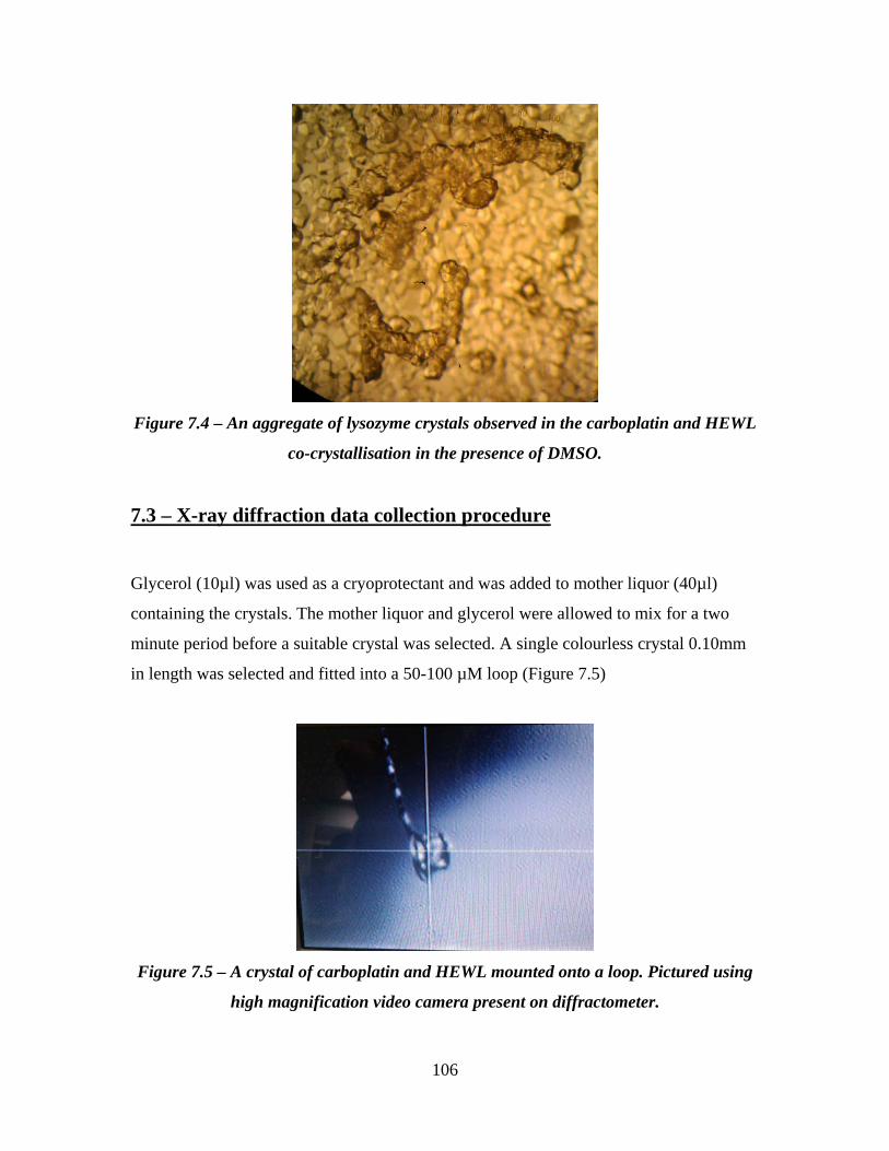
106

Figure 7.4 – An aggregate of lysozyme crystals observed in the carboplatin and HEWL

co-crystallisation in the presence of DMSO.

7.3 – X-ray diffraction data collection procedure

Glycerol (10µl) was used as a cryoprotectant and was added to mother liquor (40µl)

containing the crystals. The mother liquor and glycerol were allowed to mix for a two

minute period before a suitable crystal was selected. A single colourless crystal 0.10mm

in length was selected and fitted into a 50-100 µM loop (Figure 7.5)

Figure 7.5 – A crystal of carboplatin and HEWL mounted onto a loop. Pictured using

high magnification video camera present on diffractometer.

107

and mounted onto an R-Axis imaging plate diffractometer with a rotating copper anode.

The crystal to detector distance was set at 120mm and the data collection temperature at

100K. A full 360º of data were collected with an exposure time of six and a half minutes

per degree. Figure 7.6 is one of the X-ray diffraction images obtained. A summary of the

data collection statics is listed in Table 11.

The resulting data was processed, merged and scaled using the d*trek program36 (part of

the Rigaku suite of programs). An initial model structure was obtained using the model

replacement method. This was done using the PHASER computer program which is part

of the CCP4i suite37. The resolution of the model was solved to 2 Ǻ.


Space group P 43 21 2

Unit cell dimensions a = 77.0869 Ǻ α = 90.00°

b = 77.0869 Ǻ β = 90.00°

c = 36.4220 Ǻ γ = 90.00°

Unit cell volume 216433 Ǻ3

Data collection temperature 100 K

Radiation CuKα rotating anode

Diffractometer R-Axis

Detector Image plate

Crystal size 0.10mm x 0.10mm

Crystal mosaicity 1.737°



Data completeness 82.7% (18.6%)

<I σI> 12.7 (2.4)

Average redundancy 12.41 (4.17)

Rmerge 0.084 (0.512)

Resolution range 54.51 – 1.65 (1.71 – 1.65)

Table 11 – The summary of the X-ray diffraction data collection of HEWL and

carboplatin crystal. Values in parentheses indicate the last resolution shell

108

Figure 7.6 – An X-ray diffraction pattern image from the carboplatin & HEWL data

collection.

7.4 – Model refinement procedure

The following steps were performed to move from an initial model to a final structure.

All the refinement steps were performed in the refmac 5 program which is part of the

CCP4i suite. Map inspection and model building was performed in the COOT program38.

Step 1

A previously reported lysozyme structure was used as an initial model (PDB file

1BWJ51).

To begin with a twenty cycle rigid body refinement was performed on the protein

coordinates with overall refinement of the temperature factor.


refinement

RFree after

refinement

0.3335 0.3341 0.3335 0.3359

109

Step 2

The COOT program was used to inspect the electron density map. This revealed a good

correlation between the model and the experimentally obtained electron density. Two

peaks of 10.49 sigma and 8.29 sigma were present in the electron density map and were

assigned as platinum atoms. The occupancy of the atoms was set at 30% with a

temperature factor of 50.00. The model was then subjected to 20 cycles of restrained

refinement with isotropic refinement of temperature factors.


refinement

RFree after

refinement

0.3189 0.3161 0.2030 0.2624

Step 3

Two ammonia groups were added to one of the platinum sites in place of water

molecules. This was because the bond lengths are similar to those reported for the length

of the Pt-NH3. The occupancy of the nitrogen atoms was set at 30% and the temperature

factor at 50.00. A further ten cycles of restrained refinement was performed with

isotropic refinement of temperature factors.


refinement

RFree after

refinement

0.2036 0.2662 0.2016 0.2678

Step 4

One ammonia group was added to the other platinum site in place of a water molecule.

Again the bond length appeared consistent with the reported value of the Pt-NH3 bond.

The occupancy of the nitrogen atom was set at 30% and the temperature factor at 50.00.

A further ten cycles of restrained refinement was performed with isotropic refinement of

temperature factors.

110


refinement

RFree after

refinement

0.2014 0.2676 0.2012 0.2697

Step 5

The remaining ammonia group was added to the other platinum site in place of a water

molecule. The occupancy of the nitrogen atom was set at 30% and the temperature factor

at 50.00. A further ten cycles of restrained refinement was performed with isotropic

refinement of temperature factors.


refinement

RFree after

refinement

0.2033 0.2728 0.2020 0.2695

Step 6

The electron density around each water molecule was inspected at one sigma to make

sure the waters contained within the starting model correlated with the experimentally

determined electron density. This process resulted in the removal of 52 water molecules.

In addition 5 cycles of COOT : Find water were performed.


refinement

RFree after

refinement

0.2104 0.2720 0.2069 0.2677

Step 7

A further sixteen water molecules were deleted as well as a sodium atom. This was

because these species displayed no electron density. The final occupancy value of both

sites was set at 30% which is consistent with the cisplatin binding to HEWL as reported

by Casini et al.

111


refinement

RFree after

refinement

0.2149 0.2778 0.2133 0.2809

Further optimisation of the structure was not possible and it is noted that the RFree has

increased by around 1% from the last refinement step.

The evolution of the R factor with each step of refinement is illustrated clearly by Figure

7.7.

Figure 7.7 – A figure to illustrate the gradual reduction of the conventional R factor

with each step of refinement performed.

7.5.1 - Analysis of the three dimensional structure

From initial inspection of the electron density map it was observed that carboplatin had

bound at two distinct sites within lysozyme. The two sites were on either side of the

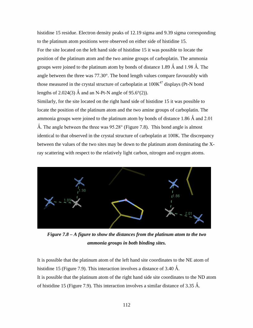
112

histidine 15 residue. Electron density peaks of 12.19 sigma and 9.39 sigma corresponding

to the platinum atom positions were observed on either side of histidine 15.

For the site located on the left hand side of histidine 15 it was possible to locate the

position of the platinum atom and the two amine groups of carboplatin. The ammonia

groups were joined to the platinum atom by bonds of distance 1.89 Ǻ and 1.98 Ǻ. The

angle between the three was 77.30°. The bond length values compare favourably with

those measured in the crystal structure of carboplatin at 100K47 displays (Pt-N bond

lengths of 2.024(3) Ǻ and an N-Pt-N angle of 95.6°(2)).

Similarly, for the site located on the right hand side of histidine 15 it was possible to

locate the position of the platinum atom and the two amine groups of carboplatin. The

ammonia groups were joined to the platinum atom by bonds of distance 1.86 Ǻ and 2.01

Ǻ. The angle between the three was 95.28° (Figure 7.8). This bond angle is almost

identical to that observed in the crystal structure of carboplatin at 100K. The discrepancy

between the values of the two sites may be down to the platinum atom dominating the X-

ray scattering with respect to the relatively light carbon, nitrogen and oxygen atoms.

Figure 7.8 – A figure to show the distances from the platinum atom to the two

ammonia groups in both binding sites.

It is possible that the platinum atom of the left hand site coordinates to the NE atom of

histidine 15 (Figure 7.9). This interaction involves a distance of 3.40 Ǻ.

It is possible that the platinum atom of the right hand side site coordinates to the ND atom

of histidine 15 (Figure 7.9). This interaction involves a similar distance of 3.35 Ǻ.

113

Figure 7.9 - A figure to show the distance from the platinum atom to the nearest

nitrogen atom on the histidine 15 residue for both binding sites.

Both sites displayed significant amounts of electron density (Figure 7.10 & Figure 7.11)

but with shapes that made the location of additional atoms difficult. The binding site on

the left hand side of histidine 15 appeared to more strongly defined suggesting a higher

occupancy than the site on the right hand side of histidine 15.

Figure 7.10- A figure to show the electron density around the binding site on the left

hand side of histidine 15.

114

Figure 7.11 - A figure to show the electron density around the binding site on the right

hand side of histidine 15.

7.5.2 - Comparison with HEWL and cisplatin crystal structure

The structure of HEWL and cisplatin as reported by Casini et al46 was deposited as a

PDB file under the deposition code 216Z. This PDB file was superimposed with respect

to the final version of the HEWL and carboplatin PDB. The superimposition was done

with respect to the alpha carbon atoms of lysozyme and was performed using the Lsqkab

program (which is part of the CCP4i suite). This ensured that both the structures were

arranged in the same orientation within the unit cell. The PDB was then subjected to

twenty cycles of restrained refinement with overall refinement of the temperature factor

using refmac 5. Finally, a FO-FC map was generated with peaks greater than 3sigma listed.

This was done using the FFT program (part of the CCP4i suite).

The superimposition (Figure 7.12) revealed that the positions of the majority of the amino

acid sequences, of the two PDB files closely agreed. However it appears that the histidine

15 residue is noticeably displaced (0.75 Ǻ ) in the HEWL and carboplatin model (with

respect to the HEWL and cisplatin model). It is possible that this displacement allows the

binding of the two carboplatin molecules on either side of histidine 15 as opposed to a

single cisplatin molecule.

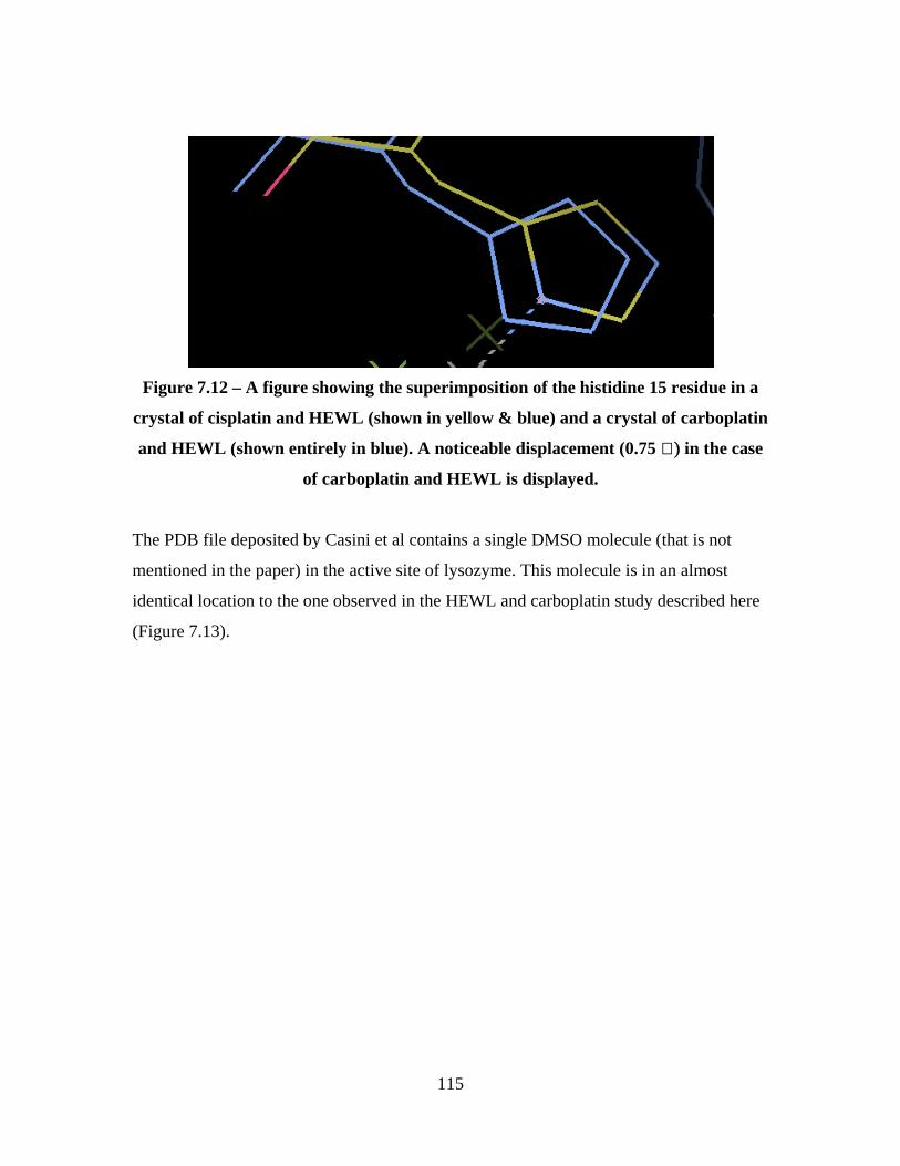
115

Figure 7.12 – A figure showing the superimposition of the histidine 15 residue in a

crystal of cisplatin and HEWL (shown in yellow & blue) and a crystal of carboplatin

and HEWL (shown entirely in blue). A noticeable displacement (0.75 Ȧ) in the case

of carboplatin and HEWL is displayed.

The PDB file deposited by Casini et al contains a single DMSO molecule (that is not

mentioned in the paper) in the active site of lysozyme. This molecule is in an almost

identical location to the one observed in the HEWL and carboplatin study described here

(Figure 7.13).

116

Figure 7.13 – A figure displaying the location of the DMSO molecule present within

the lysozyme active site for both the cisplatin and carboplatin models.

7.5.3 - Comparison with previous HEWL and carboplatin crystal structure

This work was conducted by Joanne Meredith for award of an MChem degree47. The

crystals of HEWL and carboplatin were grown using a batch method co-crystallisation in

the absence of DMSO.

In this case it was found that the carboplatin had bound at four distinct sites within

lysozyme with four peaks visible at 3.10 sigma. Interestingly, it appeared one of the

binding sites was in the sugar binding, active site of lysozyme. This is an intriguing result

as it suggests the possibility of using carboplatin to inhibit enzymes where sugar binding

is involved in the catalytic process.

Catalytic residues of lysozyme Top arrow indicates glutamic acid 135. Bottom arrow indicates aspartic acid 52.

Left hand arrow indicates the location of the sulphur atom of DMSO present in the carboplatin and HEWL model. The right hand arrow indicates the location of the DMSO molecule present in the cisplatin and HEWL model.

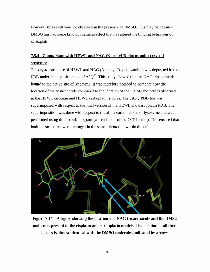
117

However this result was not observed in the presence of DMSO. This may be because

DMSO has had some kind of chemical effect that has altered the binding behaviour of

carboplatin.

7.5.4 - Comparison with HEWL and NAG (N-acetyl-D-glucosamine) crystal

structure

The crystal structure of HEWL and NAG (N-acetyl-D-glucosamine) was deposited in the

PDB under the deposition code 3A3Q52. This study showed that the NAG trisaccharide

bound to the active site of lysozyme. It was therefore decided to compare how the

location of the trisaccharide compared to the location of the DMSO molecules observed

in the HEWL cisplatin and HEWL carboplatin studies. The 3A3Q PDB file was

superimposed with respect to the final version of the HEWL and carboplatin PDB. The

superimposition was done with respect to the alpha carbon atoms of lysozyme and was

performed using the Lsqkab program (which is part of the CCP4i suite). This ensured that

both the structures were arranged in the same orientation within the unit cell

Figure 7.14 – A figure showing the location of a NAG trisaccharide and the DMSO

molecules present in the cisplatin and carboplatin models. The location of all three

species is almost identical with the DMSO molecules indicated by arrows.

118

The superimposition revealed that one end of the NAG trisaccharide is in the same

position as the DMSO molecule in both the HEWL and cisplatin and HEWL and

carboplatin studies. This may mean that the DMSO prevents the carboplatin from binding

at the active site in the manner observed in the DMSO free work conducted by Joanne

Meredith.

7.6 – Implications of the three dimensional structure

X-ray diffraction analysis of a DMSO free co-crystallisation of carboplatin and HEWL

(conducted by Joanne Meredith) revealed that the carboplatin had bound to the sugar

binding, active site of lysozyme. Binding to this site was thought to be feasible as the

bidentate dicarboxylate ligand possess a reasonable structural resemblance to that of a

sugar ring. This raised the possibility that carboplatin might act as an inhibitor for sugar

binding enzymes such as heparanase.

In an effort to increase the occupancy of the carboplatin, DMSO was introduced into a

co-crystallisation of carboplatin and HEWL. X-ray diffraction analysis revealed that the

presence of DMSO had apparently altered the binding behaviour of carboplatin. It was

found that although DMSO had improved the occupancy of the carboplatin it had also

bound to the active site. This raises the possibility that the presence of DMSO prevented

the carboplatin binding to the sugar binding, active site of lysozyme. Indeed it was found

that the DMSO bound to the same site in lysozyme as a NAG trisaccharide. From this

work it is impossible to verify if carboplatin displays binding behaviour similar to that of

sugars, possibly due to the interference of DMSO.

Instead it was found that the carboplatin bound in a similar manner to that of cisplatin (as

reported by Casini et al). However, where cisplatin had only bound to a single side of

histidine 15, it was found that carboplatin had bound to both sides. A superimposition of

the protein coordinates from the co-crystallisation of carboplatin and HEWL and those of

cisplatin and HEWL reported by Casini et al was performed. This revealed that in the co-

crystallisation of carboplatin and HEWL the histidine 15 residue was noticeably

displaced (displacement of 0.75 Ǻ ) with respect to the histidine 15 observed in the Casini

et al coordinates. This displacement may be essential in allowing the carboplatin to bind

119

at both sides of the residue as opposed to one side. However, Casini et al used a soaking

method as opposed to a co-crystallisation which may have had some bearing upon the

cisplatin and HEWL results. To confirm these apparent differences in carboplatin and

cisplatin binding to HEWL, X-ray diffraction analysis of a co-crystallisation of cisplatin

and HEWL would need to be performed.

In both of the carboplatin binding sites only the platinum atom and the two ammonia

groups could be located (achieving the same level of detail as reported by Casini et al).

120

Chapter 8

Future work

In the HEWL and Ta6Br12 co-crystallisation the location of the tantalum atoms was

relatively easy by inspection of the electron density map. This is owing to the high

amount of electron density possessed by the tantalum atoms. In contrast it was difficult to

locate the bromine positions which have a much lower electron density and scatter X-rays

more weakly. The difficulty in determining the location of the bromine atoms was

probably at least partly due to the low occupancy of the binding sites. A possible solution

would be to perform the co-crystallisation of the Ta6Br12 cluster and HEWL in the

presence of a solvent such as DMSO. This could possibly increase the solubility of the

Ta6Br12 cluster and promote increased binding.

An additional idea would be to perform the co-crystallisation at a different pH. As the

Ta6Br12 cluster is positively charged it may bind to different locations in HEWL. These

derivatives could possibly be used in the multiple isomorphous replacement method in

order to obtain a more detailed three dimensional structure.

In the carboplatin and HEWL co-crystallisation the presence of DMSO apparently

chemically altered the binding behaviour of carboplatin. The obvious suggestion would

be to repeat the co-crystallisation of carboplatin and HEWL in the presence of a different

additive. However as carboplatin is insoluble in solvents such as ethanol and acetone this

may prove difficult. If crystals in the presence of a different additive could be obtained

the possible sugar binding behaviour of carboplatin could be properly assessed.

121

References

1. Bravais lattice types image (2010), [Online] Available at:

www.schielo.cl/fbpe/img/bscq/v46n3/fig04.gif

2. Molloy, C. K., (2004), Group theory for chemists: fundamental theory and applications, Horwood

3. Hahn, T. (Ed)., (1983), International tables for crystallography (volume A), Published for the International Union of Crystallography by Reidel

4. 21 screw axis image (2010), [Online] Available at: www.axxel.iqfr.csic.es/Cristalographica/archives-07/helicodial.jpg

5. Bragg, L. W., (1983), The diffraction of short electromagnetic waves by a crystal, Proc. Camb. Phil. Soc. 17 part 1, 43-57

6. Woolfson, M. M., (1997), An introduction to X-ray crystallography (2nd edition), Cambridge University Press

7. Bragg pictorial representation (2010), [Online] Available at: http://serc.carleton.edu/images/research_education/geochemsheets/braggslaw.jpg

8. Suryanarayna, C., Norton, M. G., (1998), X-ray diffraction: A practical approach, Plenium Press

9. X-ray tube image (2010), [Online] Available at: http://pubs.usgs.gov/of/2001/of01-041/htmldocs/images/xrdtube.jpg

10. Elder, R. F., Gurewitsch, M. A., Langmui,r V. R., Pollock, H. C., (1947),

Radiation from electrons in a synchrotron, Physical review, 71, 829-830

11. Ramakanth, Hebbar, K., (2007), Basics of X-ray diffraction and its applications, I.K. International

12. Clegg, W., Blake, J. A., (2009), Crystal structure analysis: Principles and practice

(2nd edition), Oxford University Press

122

13. Helliwell, R. J., (1992), Macromolecular crystallography with synchrotron

radiation, Cambridge University Press

14. Patterson, L. A., (1935), A direct method for the determination of the component

of interatomic distances in crystals, Z. Krist, 90, 517-542

15. Bruker, (2002), Saint version 6.36a, Bruker AXS Inc.

16. Sheldrick, H. G., Schneider, R. T., (1997), SHELXL: High resolution refinement, Methods in enzymology, 277, 319-343

17. Burla, C. M., Caliandro, R., Camalli, M., Carrozzini, B., Cascarano, L. G., De Caro, L., Giacovazzo, C., Polidori, G., Spagna, R., (2005), SIR2004: An improved tool for crystal structure determination and refinement, J. Appl. Cryst, 38, 381-388

18. Das, A., Dey, B., Jana Dipankar, A., Hemming, J., Helliwell, M., Lee Man, H., Hsiao, T., Suresh, E., Colacio, E., Choudhury, R. S., Mukhopadhyay, S., (2010), Effect of protonated aminopyridines on the structural divergences of M(ΙΙ)-malonate complexes, Polyhedron, 29, 1317-1325

19. Allen H. F, (2002), The Cambridge structural database: a quarter of a million structures and rising, Acta. Cryst. B., 58 ,380-388

20. Bruno, J. I., Cole, C. J., Edgington, R. P., Kessler, M., Macrae, F. C., McCabe, P., Pearson, J., Taylor, R., (2002), New software for searching the Cambridge Structural Database and visualizing crystal structures, Acta. Cryst. B., 58, 389-397.

21. Spek, L. A., (2003), Single crystal structure validation with the program PLATON, J. Appl. Cryst., 36, 7-13.

22. Chieh, C. P., Trotter, J., (1970), Crystal structure of tetraphenyltin, J. Chem. Soc. 6, 911-914.

23. (2010), [Online] Available at: http://nobelprize.org/nobel_prizes/chemistry/laureates/2009/

24. (2010), [Online] Available at www.pdb.org

123

25. Blundell, L. T., Johnson, N. L., (1976), Protein crystallography, Academic Press, 69-77

26. Chayen, N., Comparative studies of protein crystallization by vapour diffusion and micro batch techniques, Acta Cryst D, 54(1), 8-15

27. King, V. M., (1965), A low resolution structural model for cubic glucagon based on the packing of cylinders, J. Mol. Biol, 11, 549-561

28. Evans, P., McCoy, A., (2008), An introduction to molecular replacement, Acta Cryst D, 64, 1-10

29. Alberts, B., Johnson, A., Lewis, J., Raff, M., Roberts, K., Walter, P., (2002), Molecular biology of the cell (4th edition), Garland Science

30. Stryer, L., Berg, M. J., Tymoczko, L. J., (2006), Biochemistry (6th edition), W. H. Freeman

31. Yonath, A et al., (2005), Crystallographic studies on the ribosome, a large

macromolecular assembly exhibiting severe nonisomorphoism, extreme beam sensitivity and no internal symmetry, Acta. Cryst A. 54, 945-955

32. Knablein, J et al., (1997), Ta6Br122+, a tool for phase determination of large

biological assemblies by X-ray crystallography, J. Mol. Biol. 270, 1-7.

33. Szcezepanowski, H. R., Filipek, R., Bochtler, M., (2005), Crystal structure of mouse ubiquitin activating enzyme, J. Biol. Chem. 280, 22006-22011

34. (2010) Jena Bioscience tantalum cluster derivatization user guide, [Online] Available at: www.jenabioscience.com

35. Corey, B. R., Stanford, H. R., Marsh, E. R., Leung, C. Y., Kay, M. L., (1962), An

X-ay investigation of wet lysozyme chloride crystals, Acta Cryst, 15, 1157-1163

36. Pflugrath, W. J., (1999), The finer things in X-ray diffraction data collection, Acta Cryst D, 55, 1718-1725

37. Collaborative, (1994), The collaborative computational project number 4:

programs for protein crystallography, Acta. Cryst. D., 50(5), 760-763

124

38. Emsley, P., Lohkamp, P., Scott, W., Cowtan, K., (2010), Features of Coot, Acta.

Cryst. D., In press.

39. PDB ID = 2W1Y Cianci, M., Helliwell R. J., Suzuki, A., (2008), The interdependence of wavelength. Redundancy and dose is sulphur SAD experiments, Acta Cryst D, 64, 1196-1209

40. Vojnovic, M., Brnicevic, N., Basic, I., Planinic, P., Giester, G., (2002), The Co crystallization of the Cubic [Ta6Br12(H2O)6][CuBr2X2]·10H2O and Triclinic [Ta6Br12(H2O)6]X2·trans-[Ta6Br12(OH)4(H2O)2]·18H2O (X = Cl, Br, NO3) Phases with the Coexistence of [Ta6Br12]2+ and [Ta6Br12]4+ in the Latter, ZAAC, 628, 401-408

41. Kumar, Y. S., (2009), X-ray crystal structure analyses of small and large molecules (Msc thesis), The University of Manchester

42. Rosenberg, B., Van Camp, L., Krigas, T., (1965), Inhibition of cell division in

Escherichia Coli by electrolysis products from a platinum electrode, Nature, 205, 698-699

43. Skeel, T. R. (Ed), Handbook of cancer chemotherapy (6th edition), Lippincott Williams and Wilkins.

44. Pratt, B. W., Ruddon, W. R., (1979), The anticancer drugs, Oxford University press.

45. Takahara, T., Rosenweig, C. A., Frederick, A. C., Lippard, J. S., (1995), Crystal

structure of double-stranded DNA containing the major adduct of the anticancer drug cisplatin, Nature, 377, 649-652

46. Casini, A., Mastrobuoni, G., Temperini, C., Gabbiani, C., Francese, S., Moneti, G., Supuran, T. C., Scozzfava, A., Messori, L., (2006), ESI mass spectrometry and X-ray diffraction studies of adducts between anticancer platinum drugs and hen egg white lysozyme, Chem. Commun, 2,156-158,

47. Meredith, J., (2010), The University of Manchester (MChem dissertation),

48. Carboplatin (2010), [Online] Available at:

125

www.tocris.com/dispprod.php?ItemId=5205

49. Lehmann, S. M,. Stansfield, D. F. R., (1989), Binding of dimethyl sulfoxide to lysozyme crystals, studied with neutron diffraction, Biochemistry, 28, 7028-7033

50. Lu, J., Wang, J. X,. Ching, B. C., (2002), Effect of additives on the crystallization of lysozyme and chymotrypsinogen A, Crystal growth & design, 3(1), 83-87

51. PDB ID = 1BWJ Dong, J., Boggon, J. T., Chayen, E. N., Raftery, J., Bi, C. R., Helliwell, R. J., (199), Bound solvent structures for microgravity, ground control, gel and microbatch grown hen egg white lysozyme crystals at 1.8Ȧ resolution, Acta Cryst D. 55 745-752

52. PDB ID = 3A3Q

Ose, T., Kuroki, K., Matsushima, M., Maenaka, K., Kumagai, I., (2009), Importance of the hydrogen bonding network including Asp 52 for catalysis, as revealed by Asn 59 mutant hen egg white lysozyme, J Biochem, 146, 651-657

126

Bibliography

• Blow, D., (2002), Outline of crystallography for biologists, Oxford University

Press • Clegg, W., (1998), Crystal structure determination, Oxford University Press • Glusker Pickworth, J., Trueblood, N. K., (1985), Crystal structure analysis,

Oxford University Press • Arndt, W. U., Willis, M. T. B., (1996), Single crystal diffractometery,

Cambridge University Press • Woolfson, W. M., (1997), An introduction to X-ray crystallography,

Cambridge University Press • Blundell, T. L., Johnson, N. L., (1976), Protein crystallography, Academic

Press Inc • McPherson, A., (1982), Preparation and analysis of protein crystals, John

Wiley & Sons • Ramakanth, Hebbar, K., (2007), Basics of X-ray diffraction and its

applications, I.K. International

• Helliwell, R. J., (1992), Macromolecular crystallography with synchrotron

radiation, Cambridge University Press

Structure determination of small and large molecules by ...

Documents

Transcript of Structure determination of small and large molecules by ...