Structure and Propagation of ... - Princeton University
143
1 Structure and Propagation of Turbulent Premixed Flames Swetaprovo Chaudhuri Associate Professor University of Toronto Institute for Aerospace Studies 2021 Princeton-Combustion Institute Summer School on Combustion
Transcript of Structure and Propagation of ... - Princeton University
1
Structure and Propagation of
Turbulent Premixed Flames
Swetaprovo Chaudhuri
Associate Professor
University of Toronto Institute for Aerospace Studies
2021 Princeton-Combustion Institute Summer School on Combustion

Outline
i. Introduction
ii. Regime Diagrams
iii. Evolution of Flame Surfaces in Moderate Turbulence
iv. Local Flame Speed and Structure in Moderate and Intense
Turbulence
v. Turbulent Flame Speed
vi. Turbulence-DL Instability Interaction

Three faces of a flame

4
Turbulent Premixed Flames in Engineering DevicesTurbulent premixed combustion• SI engines• Gas turbine engines: aircrafts (partially
premixed) and stationary power systems
• Industrial gas burners• Vapor cloud explosions• Supernova Ia
DNStostudyinteractionofturbulencewithfreelypropagatingpremixedflame
LPP Combustor
[1] Driscoll, J. and Temme, J., 2011, January, 49th AIAA Aerospace Sciences Meeting including the New Horizons Forum and Aerospace Exposition(p.108).[2] Video Courtesy: Prof. Hong Im

5
Regime Diagrams
Comparison of characteristic length-scales and time-scalesin turbulent flow with the corresponding scales of chemicalreaction and laminar flame
Length-scales and time-scales in laminar flame:ℓ" = ⁄a 𝑆" , 𝜏" = ⁄a 𝑆" (
In turbulent flow field, length-scales and time-scales cancorrespond to Integral scales or Kolmogorov micro-scales
Comparison of scales helps in assessing whether a laminarflame structure can exist in a turbulent flow

6
Regime Diagrams
Assumptions:• 𝑆𝑐 = 1, 𝑃𝑟 = 1• The regimes so defined are only tentative and are not be
taken as strict demarcations
Some important non-dimensional numbers are obtainedon comparison of scales between turbulence and laminarflame, which help in making the regime diagram
𝜈 = 𝐷= a, which leads to 𝜈 = ℓ"𝑆" and therefore
𝑅𝑒1 =𝑢13 ℓ1ℓ"𝑆"
(1)

Regime Diagrams: invoking Kolmogorov’s similarity hypotheses
Pope, S.B., 2001. Turbulent flows.

8
Regime Diagrams: invoking Kolmogorov’s 1st similarity hypothesis
Turbulent 𝐾𝑎 = ⁄𝜏" 𝜏6Using 𝑅𝑒6 = 1 and 𝜈 = a = 𝐷, we get 𝐾𝑎 = ⁄ℓ" 𝜂 (; 𝐾𝑎𝑅 = ⁄ℓ8 𝜂 (
Using ⁄𝜂 ℓ1 = 𝑅𝑒1⁄9: ; and 𝑅𝑒1 =
<=> ℓ=ℓ?@?
, we get
Turbulent 𝐷𝑎 = ⁄𝜏1 𝜏"Using 𝜏1 = ⁄ℓ1 𝑢13 and 𝜏" = ⁄ℓ" 𝑆", we get
𝐾𝑎( =ℓ1ℓ"
9A 𝑢13
𝑆"
:(2)
𝐷𝑎 =ℓ1ℓ"
𝑢13
𝑆"
9A(3)

9
Interpretation of 𝐾𝑎 and 𝐷𝑎
𝐷𝑎 helps in assessing interaction of large scales (of theorder of Integral scales) of turbulence with the flame
𝐷𝑎 ≫ 1 ⇒ flame time-scales are smaller than large time-scales in turbulence and it is difficult for large scales todisturb flame structure
𝐾𝑎 helps in assessing interaction of small scales (of theorder of Kolmogorov micro-scales) of turbulence with theflame𝐾𝑎 ≪ 1 ⇒ flame time-scales are smaller than Kolmogorovtime-scales in turbulence and it is difficult for small scalesto disturb flame structure

Regime Diagrams
The regime diagram shown above is one example. Otherregime diagrams also exist
𝐾𝑎8 = 1, 𝜂 = ℓ8
𝐾𝑎" = 1, 𝜂 = ℓ"
⁄ℓE ℓ"
Peters, N., 2001. Turbulent combustion.

11
Regime Diagrams
Wrinkled flamelet regime: (𝑅𝑒 > 1, 𝐾𝑎" < 1, ⁄𝑢E3 𝑆" < 1)• ℓ" < 𝜂 ⇒ flame element retains laminar flame structure within
turbulent flow field• 𝑢E3 < 𝑆" ⇒ flamelet surface is only slightly wrinkled
Corrugated flamelet regime: 𝑅𝑒 > 1,𝐾𝑎" < 1, ⁄𝑢E3 𝑆" > 1• ℓ" < 𝜂 ⇒flame element retains laminar flame structure• 𝑢E3 > 𝑆" ⇒ flamelet surface is highly convoluted

Regime Diagrams
Reaction-sheet regime: 𝑅𝑒 > 1,𝐾𝑎" < 1, 𝐾𝑎8 < 1• Eddies smaller than ℓ" penetrate the preheat zone; for large eddies
flame is still a flamelet• Reaction sheet thickness ℓ8 < 𝜂 ⇒ reaction sheet is only wrinkled
Well-stirred reactor regime: 𝑅𝑒 > 1,𝐾𝑎8 > 1• Entire flow field behaves like a well-stirred reactor without any
distinct local flame structure

Genesis and Evolution of Premixed Flames in Moderate Turbulence
13

Laminar vs. Turbulent Premixed Flames
14
Standard Premixed Flame[1]Turbulent Premixed Flame
[1] Law, C.K., 2010. Combustion physics. Cambridge university press.[2] Video courtesy: Prof. Hong Im

15
§ Turbulent flame surfaces are continuously generated andannihilated.
§ Exact locations on a surface that generate complete newsurfaces are not known a priori – need to look back in time.
Objectives• Where do the fully developed, complete turbulent premixed
flame surfaces evolve from? What are their special features?• How do the flame surfaces generate and annihilate?• What implication does generation and annihilation hold for
local flame speed 𝑆J?
Objectives
Video courtesy: Prof. Hong Im

Zeldovich’s Theory of “Pilot Points”
16
“The pilot point in a non-stationary flame is the most forward-lying point of the flame front in the direction of combustionpropagation. The igniting “impulse” is transmitted from it toadjacent portions of the flame, and so on, until the flame frontencompasses the entire mixture volume…[pilot points]establish the relationship between an integral characteristic ofthe process (the surface area of the flame) and a local quantity(the maximum velocity of the gas along the tube).”[1]
Concept of leading points is valid for laminar flames[2]
Is concept of leading points valid for turbulent flames?
[1] Zeldovich, I.A., Barenblatt, G.I., Librovich, V.B. and Makhviladze, G.M., 1985. Mathematical theory of combustion and explosions.[2] Amato A., Lieuwen T., Analysis of flamelet leading point dynamics in an inhomogeneous flow, Combustion and Flame, 2014
Leading point
Fresh reactants Burned products
Flame front
Current studies assume definition of leading points

Flame Particle Tracking
𝜕𝒙N 𝑿N 𝜓1 , 𝑡𝜕𝑡
= 𝒗N 𝑿N 𝜓E , 𝑡 = 𝒖N + 𝑆JN𝒏N
Pope, S.B., 1988, International journal of engineering science, 26(5), pp.445-469.Chaudhuri, S., 2015, Proceedings of the Combustion Institute, 35(2), pp.1305-1312.

Computational Details DNS-Backward Flame Particle Tracking Methodology
18
DNS of statistically planar flames
Snapshots of DNS saved at fine time
interval
Snapshots are fed to the BFPT algorithm
in reverse order
• Flame particles[1] are a class of surface points[2] that co-move with an iso-scalar surface within the flame
• Provide spatio-temporal details of specific regions of a flame
• Ensemble of flame particles forms a flame surface and ensemble of flame surfaces forms a premixed flame
What are flame particles?
Pope, S.B., 1988, International journal of engineering science, 26(5), pp.445-469.Chaudhuri, S., 2015, Proceedings of the Combustion Institute, 35(2), pp.1305-1312.

Computational MethodsDirect Numerical Simulations (DNS)
19
§ DNS Configuration§ Statistically planar flames of H2-air mixture with 𝜙 = 0.81 and 𝑃 = 1atm§ Detailed H2-air reaction mechanism[1] of 9 species and 21 reactions
P = 1atm
Isotropic turbulence box of fresh reactants
Flame Domain
𝑇E = 665𝐾Isotherm
Parameter Case-1 Case-2𝑇<, K 310 310𝐿^, cm 1.918 1.2𝐿_, cm 0.48 0.4
𝑁^, 960 384𝑁_, 240 128
ℓE, cm 0.3 0.26𝑢E, cm/s 642 662𝑢E/𝑆" 3.5 3.6𝑅𝑒E 875 782𝑘cd^𝜂 2.5 1.7𝐷𝑎 2.4 2.0𝐾𝑎 16.7 15.2
Both cases belong to the thin-reaction zone regime
[1] Li, J., Zhao, Z., Kazakov, A. and Dryer, F.L., 2004, International journal of chemical kinetics, 36(10), pp.566-575.

Results & Discussions1. Where do the flame surfaces evolve from?
Arrow of timeProgress of BFPT
𝑡e 𝑡f
Uniform distribution of flame particles over flame surface
Multiple clusters in leading regions of flame surface
Dave, H.L., Mohan, A. and Chaudhuri, S., 2018, Combustion and Flame, 196, pp.386-399.

Results & Discussion1. Features of the Multiple Clusters of Flame Particles – Leading Points
21
time 𝑡e 𝑡g 𝑡f
Clusters of flame particles are leading towards fresh reactants
Low fluid flow velocity

Results & Discussion1. Features of the Multiple Clusters of Flame Particles – Leading Points
22
Clusters are positively curved (convex towards fresh reactants)
Clusters are positively stretchedContribution of 2𝑆JN𝜅cN changes in time
and limits stretch-rate
Stretch-rate
𝐾 =1𝛿A
𝑑(𝛿𝐴)𝑑𝑡 = 𝑎n + 2𝑆J𝜅c
Strong resemblance between leading clusters of flame particles and concept of leading points by Zeldovich & co-
workers
time 𝑡e 𝑡g 𝑡f

Results & DiscussionMechanism of flame surface generation
23
time 𝑡e 𝑡g 𝑡f

Results & DiscussionFlame Particle Dispersion Statistics
24
§ The dispersion of flame particles for both sets follow modifiedBatchelor’s dispersion law[1], where 𝐶( depends on isotherm
𝚫N − 𝚫EN( =
113 𝐶( ΔEN𝜖
(:𝑡(
Set-G Set-D
[1] Chaudhuri, S., 2015, Physical Review E, 91(2), p.021001.
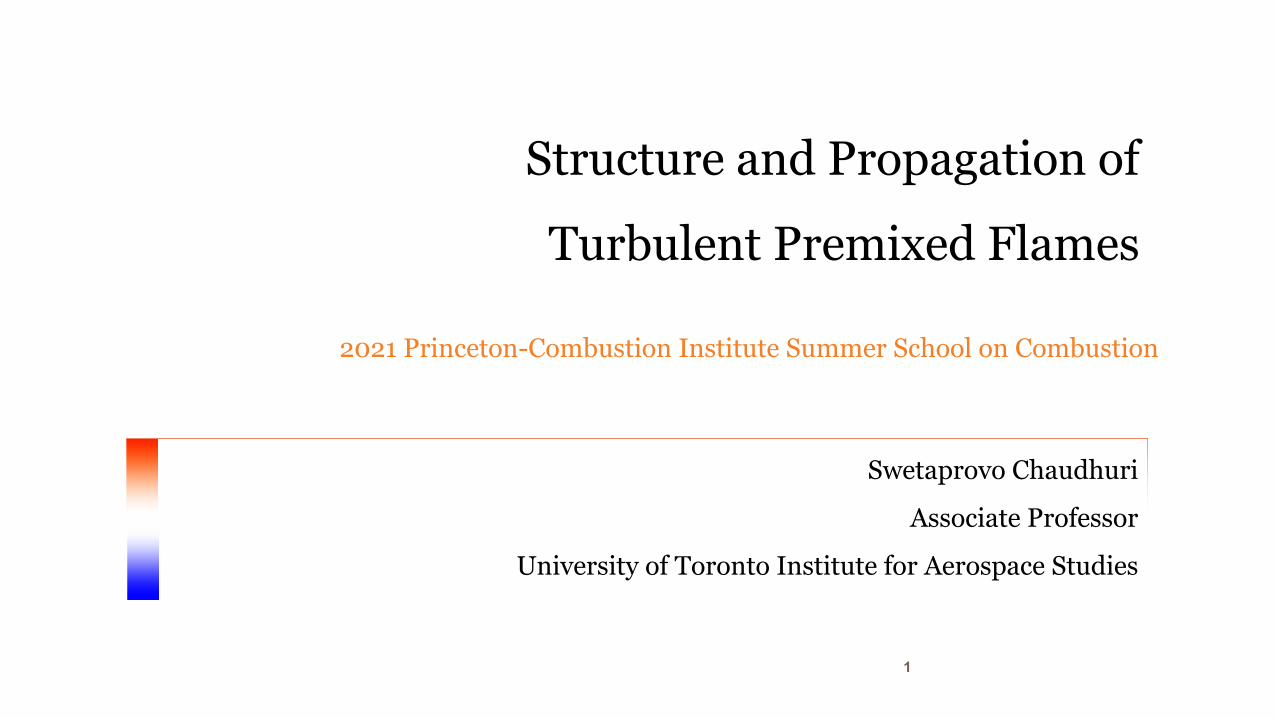
Interim Summary
25
DNS of statistically planar flames
Snapshots of DNS saved at fine time
interval
Snapshots are fed to the BFPT algorithm
in reverse order
Source location of turbulent flame
surfaces
• Fully developed turbulent flame surfaces evolve from multiple leading points
• Leading locations stretch due to • 2𝑆J𝜅c along direction of maximum curvatureu𝒆A• 𝑎n along direction of minimum curvature u𝒆(
• Relationship is developed between 𝑆n(𝑡f) and the local 𝑆J 𝑡g• Flame particles disperse as per modified Batchelor’s law• Dispersion is due to
• Flame propagation upto the Gibson scale ⁄𝑆": ⟨𝜖⟩• Turbulence beyond the Gibson scale

Evolution of Local Flame Displacement Speeds in Moderate and Intense Turbulence
Flame displacement speed (Sd): Speed with which a flame surface propagates, locally, relative to the local flow velocity in the direction of the local surface normal vector

27
Local Flame Speeds
Flame Consumption Speed:
𝑆g =∫z 𝜔N 𝑑Ω𝜌𝑌N ��dg𝐴��f
Flame Displacement Speed:𝑆J = (𝒗N−𝒖). 𝒏
𝑆J𝒏(𝒙, 𝑡)
𝒖(𝒙, 𝑡)
𝒗N(𝒙, 𝑡)
Flame surface
28
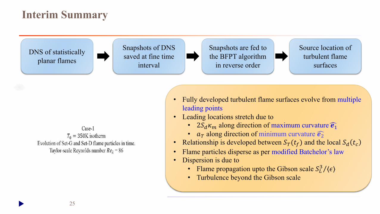
G-equation
Equation governing a propagating surface in a flow𝐺 𝒙, 𝑡 = 0 as the geometry of surface𝐺 < 0 as reactants𝐺 > 0 as products𝑆J is local flame displacement speed along 𝒏𝒏 is local normal to surface, where 𝒏 = ⁄−𝛁𝐺 𝛁𝐺
unburned gas𝐺 < 0
Burned gas𝐺 > 0
𝑆J𝒏(𝒙, 𝑡)
𝐺 𝒙, 𝑡 = 0
𝒖(𝒙, 𝑡)
Kerstein, A.R., Ashurst, W.T. and Williams, F.A., 1988, Physical Review A, 37(7), p.2728.
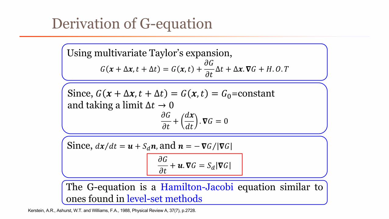
Derivation of G-equation
Using multivariate Taylor’s expansion,𝐺 𝒙 + ∆𝒙, 𝑡 + ∆𝑡 = 𝐺 𝒙, 𝑡 +
𝜕𝐺𝜕𝑡∆𝑡 + ∆𝒙. 𝛁𝐺 + 𝐻.𝑂. 𝑇
Since, 𝐺 𝒙 + Δ𝒙, 𝑡 + Δ𝑡 = 𝐺 𝒙, 𝑡 = 𝐺E=constantand taking a limit ∆𝑡 → 0
𝜕𝐺𝜕𝑡
+𝑑𝒙𝑑𝑡
. 𝛁𝐺 = 0
Since, ⁄𝑑𝒙 𝑑𝑡 = 𝒖 + 𝑆J𝒏, and 𝒏 = − ⁄𝛁𝐺 𝛁𝐺𝜕𝐺𝜕𝑡
+ 𝒖. 𝛁𝐺 = 𝑆J 𝛁𝐺
The G-equation is a Hamilton-Jacobi equation similar toones found in level-set methods

IntroductionMotivation
§ Flame displacement speed 𝑆J§ manifestation of chemical reactions
and diffusion processes within apremixed flame
§ crucial parameter in flame-fronttracking methods[1-3]
𝜕𝐺𝜕𝑡
+ 𝒖 ⋅ 𝛁𝐺 = 𝑆J 𝛁𝐺𝜕Σ𝜕𝑡+ 𝛁 ⋅ 𝒖 + 𝑆J𝒏 �Σ = 𝐾 �Σ
§ related to turbulent flame speed 𝑆n
𝑆n =1𝐴"���𝑆J𝑑𝐴
§ How do flames respond to strainand curvature effects in turbulence?
Turbulent flame iswrinkled &
stretched at many length- and time-
scales
Ensemble of perturbed flamelets
Perturbed flamelets are modeled using stretched laminar
flame models
Thermal Chemical
[1] Peters, N., 2001. Turbulent combustion.[2] Poinsot, T.J. and Veynante, D., 2005. Theoretical and Numerical Combustion, Philadelphia, PA, USA[3] Veynante, D. and Vervisch, L., 2002, Progress in energy and combustion science, 28(3), pp.193-266.

IntroductionModelingEffortsOverLastEightDecadesforLaminarFlames
1940s
1960s
1980s
2000 -present
Darrieus[1] & Landau[2]
Markstein[3]
Asymptotic[4,5] & integral analysis[6,7] of stretched laminar
premixed flames
Current understanding[8,9]
𝑆J = 𝑆" at each point on the flameStability of planar premixed flame
𝑆J = 𝑆" − 𝐶𝜅Effect of curvature
𝐶 is phenomenological coefficient
𝑆J = 𝑆" − ℒ𝐾Effect of strain and curvature
ℒ is Markstein length and 𝐾 stretch-rate
�𝑆J = 𝑆" − ℒ�𝐾 − ℒ� 𝑆"𝜅Two-parameter Markstein length model
ℒ� - stretch Markstein lengthℒ� - curvature Markstein length
[1] Darrieus, G., 1938. Unpublished work; presented at la Technique Moderne (Paris) [2] Landau, L.D., 1944. Acta Physicochim USSR 77, 77-85[3] Markstein, G.H., 1964. Nonsteady Flame Propagation: AGARDograph, Macmillan, New York[4] Matalon, M. and Matkowsky, B.J., 1982. J. Fluid Mech. 124, 239-259[5] Pelce, P. and Clavin, P. 1982. J. Fluid Mech. 124, 219-237 [6] Chung, S.H. and Law, C.K., 1988. Combust. Flame, 72, 325-336. [7] De Goey, L.P.H. and ten Thije Boonkkamp, J.H.M., 1999, Combust. Flame, 119(3), pp.253-271.[8] Bechold, J.K. and Matalon, M., 2001. Combust. Flame 127 (1-2) 1906-1913[9] Giannakopoulos, G.K., Gatzoulis, A., Frouzakis, C.E., Matalon M. and Tomboulides, A.G., 2015. Combust. Flame 162 (4), 1249-1264
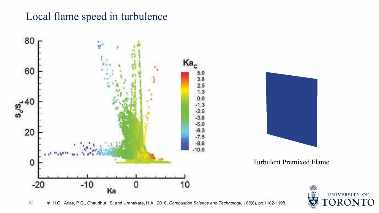
Local flame speed in turbulence
32
Standard Premixed Flame Turbulent Premixed Flame
SL
Im, H.G., Arias, P.G., Chaudhuri, S. and Uranakara, H.A., 2016, Combustion Science and Technology, 188(8), pp.1182-1198.

IntroductionStateoftheartpriorto2020§ Chen and Im (1998, 2000)[1,2] observed a wide distribution of Sd in
turbulence.§ Hawkes and Chen (2005)[3] stated that “….. steady and/or small
curvature models are unlikely to be successful for modelling thestretch response of premixed flame”
§ Chakraborty et. al. (2007)[4] stated that “there remains a need tomodel the curvature response of the combined reaction and normaldiffusion components of 𝑆J to account properly for curvature stretcheffects”
§ Recently, Im et. al. (2016)[5] have highlighted on the need tounderstand the greater excursions of local 𝑆J, questioning the validityof 𝑆J − 𝐾 relations based on laminar flame theory
[1] Chen, J.H. and Im, H.G., 1998. Symp. (Int.) Combust. 27 (1), 819-826[2] Chen, J.H. and Im, H.G., 2000. Proc. Combust. Inst. 28 (1), 211-218[3] Hawkes, E.R. and Chen, J.H., 2005. Proc. Combust. Inst. 30 (1), 647-655 [4] Chakraborty, N., Klein, M. and Cant, R.S., 2007. Proc. Combust. Inst. 31 (1), 1385-1392[5] Im, H.G., Arias, P.G., Chaudhuri, S. and Uranakara, H.A., 2016. Combust. Sci. Technol. 188 (8), 1182-1198

Computational MethodsDirect Numerical Simulations (DNS)
34
§ DNS Configuration§ Statistically planar flames of H2-air mixture with 𝜙 = 0.81 and 𝑃 = 1atm§ Detailed H2-air reaction mechanism[1] of 9 species and 21 reactions
P = 1atm
Isotropic turbulence box of fresh reactants
Flame Domain
𝑇E = 665𝐾Isotherm
Parameter Case-L Case-H𝑇<, K 310 310𝐿^, cm 1.918 2.014𝐿_, cm 0.48 0.504
𝑁^, 960 1008𝑁_, 240 252
ℓE, cm 0.31 0.33𝑢E, cm/s 670 822𝑢E/𝑆" 3.62 4.5𝑅𝑒E 950 1261𝑘cd^𝜂 2.8 2.5𝐷𝑎 2.4 2.0𝐾𝑎 13 18
Both cases belong to the thin-reaction zone regime
[1] Li, J., Zhao, Z., Kazakov, A. and Dryer, F.L., 2004, International journal of chemical kinetics, 36(10), pp.566-575.
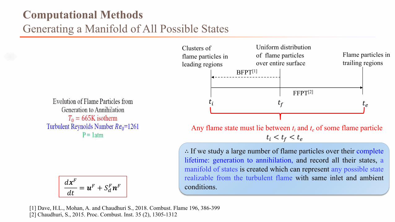
Computational MethodsGenerating a Manifold of All Possible States
𝑡e 𝑡f 𝑡�
BFPT[1]
FFPT[2]
Uniform distribution of flame particlesover entire surface
Clusters of flame particles in leading regions
Flame particles in trailing regions
Any flame state must lie between ti and te of some flame particle
∴ If we study a large number of flame particles over their completelifetime: generation to annihilation, and record all their states, amanifold of states is created which can represent any possible staterealizable from the turbulent flame with same inlet and ambientconditions.
𝑡e < 𝑡f < 𝑡�
𝑑𝒙N
𝑑𝑡= 𝒖N + 𝑆JN𝒏N
[1] Dave, H.L., Mohan, A. and Chaudhuri S., 2018. Combust. Flame 196, 386-399[2] Chaudhuri, S., 2015. Proc. Combust. Inst. 35 (2), 1305-1312
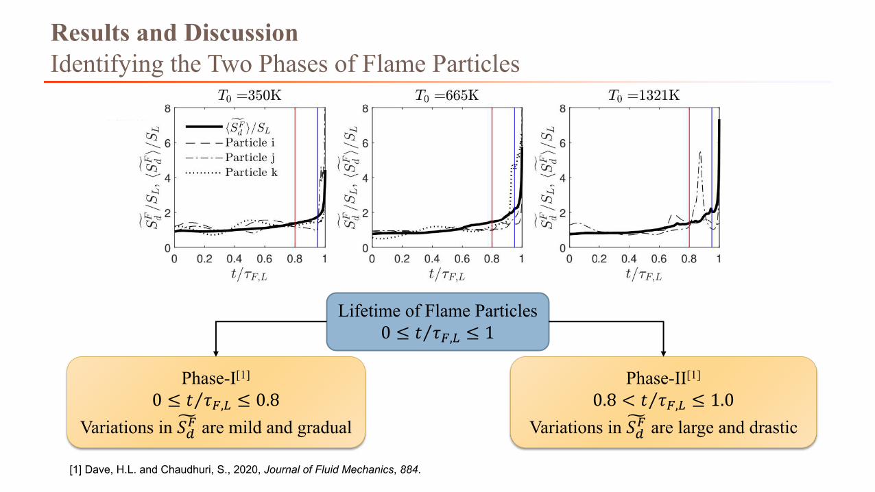
Results and DiscussionIdentifying the Two Phases of Flame Particles
Lifetime of Flame Particles0 ≤ ⁄𝑡 𝜏N," ≤ 1
Phase-I[1]
0 ≤ ⁄𝑡 𝜏N," ≤ 0.8Variations in �𝑆JN are mild and gradual
Phase-II[1]
0.8 < ⁄𝑡 𝜏N," ≤ 1.0Variations in �𝑆JN are large and drastic
[1] Dave, H.L. and Chaudhuri, S., 2020, Journal of Fluid Mechanics, 884.

Results and DiscussionPhase-I: Application of the Two-parameter Markstein Length Model§ Two-parameter Markstein length model[1]
§ Different definitions for stretch-rate exists§ Full stretch-rate: 𝐾 = 𝛁 ⋅ 𝒖 − 𝒏𝒏:𝛁𝒖 + 𝑆J𝜅
§ Asymptotic stretch-rate: 𝐾∗ = −𝒏𝒏:𝛁𝒖 + 𝑆"𝜅
§ New stretch-rate: 𝐾3 = 𝛁 ⋅ 𝒖 − 𝒏𝒏:𝛁𝒖 + 𝑆"n�n�
𝜅
�𝑆JN
𝑆"=1 − ⁄ℒ�𝑎nN 𝑆" − ℒ�𝜅N
1 + 𝜃ℒ�𝜅N(2)
�𝑆JN
𝑆"= 1 −
ℒ�𝐾∗N
𝑆"− ℒ�𝜅N (3)
�𝑆J 𝜃 = 𝑆" − ℒ� 𝜃 𝐾 − ℒ� 𝜃 𝑆"𝜅 (1)ℒ� = 𝛼 − �
A
�𝜆(𝑥)𝑥
𝑑𝑥 − ��
�𝜆(𝑥)𝑥 − 1
𝑑𝑥
𝛼 =𝜎
𝜎 − 1�A
�𝜆(𝑥)𝑥 𝑑𝑥 +
𝛽(𝐿𝑒� − 1)2(𝜎 − 1) �
A
�
ln𝜎 − 1𝑥 − 1
𝜆(𝑥)𝑥 𝑑𝑥
Stretch Markstein length
ℒ� = ��
�𝜆(𝑥)𝑥 − 1
𝑑𝑥
Curvature Markstein length
𝑻𝟎(K) ℒ�(cm) ℒ�(cm)350 -5.98×10⁹: +1.60×10⁹(
665 -1.32×10⁹: +9.26×10⁹:
1321 +3.62×10⁹; +4.24×10⁹:
Global reaction model quantities from Sun et. al.[2]
�𝑆JN
𝑆"= 1 −
ℒ�𝑆"𝑎n − ℒ�
𝑇E𝑇<+ ℒ� 𝜅N (4)
[1] Giannakopoulos, G.K., Gatzoulis, A., Frouzakis, C.E., Matalon, M. and Tomboulides, A.G., 2015. Combust. Flame 162 (4), 1249-1264[2] Sun, C.J., Sung, C.J., He, L. and Law, C.K., 1999. Combust. Flame 118 (1-2), 236-248

Results and DiscussionComparison of Theory with DNS
�@!"
@#= 1 − ℒ$�∗"
@#− ℒ�𝜅N (3)
�𝑆JN
𝑆"= 1 −
ℒ�𝑆"𝑎n − ℒ�
𝑇E𝑇<+ ℒ� 𝜅N (4)
�𝑆JN
𝑆"=1 − ⁄ℒ�𝑎nN 𝑆" − ℒ�𝜅N
1 + 𝜃ℒ�𝜅N(2)
234
234
234
234
234
234

Results and DiscussionError Estimates
�@!"
@#= 1 − ℒ$�∗"
@#− ℒ�𝜅N (3)
�𝑆JN
𝑆"= 1 −
ℒ�𝑆"𝑎n − ℒ�
𝑇E𝑇<+ ℒ� 𝜅N (4)
�𝑆JN
𝑆"=1 − ⁄ℒ�𝑎nN 𝑆" − ℒ�𝜅N
1 + 𝜃ℒ�𝜅N(2)
Phase-I Phase-II
234
234
234
234

Results and DiscussionMarkstein Length Model – Applicability and Issues
�𝑆J = 𝑆" − ℒ�𝐾 − ℒ� 𝑆"𝜅 (1)
Large stretch-rates are mostly found in regions in large negative curvature
One-timeJointProbabilityDensityFunction
1 1
1

Thermal Chemical
Flame structure in moderate turbulence
Chemical
Thermal
Dave, H.L. and Chaudhuri, S., 2020, Journal of Fluid Mechanics, 884.

§ GoverningEquations𝜌𝐶§
𝜕𝑇𝜕𝑡 =
1𝑟𝜕𝜕𝑟 𝜆𝑟
𝜕𝑇𝜕𝑟 + 𝑞𝑤
𝜌𝜕𝑌𝜕𝑡 =
1𝑟𝜕𝜕𝑟 𝜆𝑟
𝜕𝑌𝜕𝑟 − 𝑤
§ BoundaryConditionsAt𝑟 = 0,ªn
ª�= 0 andª«
ª�= 0 for𝑡 ≥ 0
At𝑟 = +∞,𝑇 = 𝑇® and𝑌 = 0 for𝑡 ≥ 0
§ InitialCondition:Whenflameissufficientlyfarfromcenter𝑟 = 0,stationarycylindricalflamesolutionisapplicable
§ Inthepreheatzone,unsteadyanddiffusionprocessesdominateandbalance
Results and DiscussionProblem: Unsteady Inwardly Propagating Cylindrical Premixed Flame

𝜌𝐶§𝜕𝑇𝜕𝑡 = 𝜆
𝑑(𝑇𝑑𝑟( +
𝜆𝑟𝑑𝑇𝑑𝑟
§ Using a stretched coordinate 𝜉 = 𝑟/𝑟f, and 𝜃 = ⁄𝑇E − 𝑇 𝑇E − 𝑇< , 𝑇E is the isotherm at the boundary of preheat & reaction zone
𝜕𝜃𝜕𝑡 −
𝜉��f𝑟f𝜕𝜃𝜕𝜉 =
𝛼<𝑟f(
1𝜉𝜕𝜃𝜕𝜉 +
𝜕(𝜃𝜕𝜉(
§ Integrating above equation for 𝜉 = 0 to 1, and simplifying using 𝜃 𝜉 = 𝜉 − 1 𝜃° and 𝜃± 𝜉 = 𝜉 − 1 ��°
��°(1)6
+��f𝑟f
𝜃°(1)3
= −𝛼<𝑟f(𝜃°(1)
§ To estimate ��° and 𝜃°, we have to analyze the reaction zone§ When 𝑟f ≫ 𝛿8, reaction zone is quasi-planar and quasi-steady, and diffusion and
reaction terms dominate and balance
Results and DiscussionProblem-2: Unsteady Inwardly Propagating Cylindrical Premixed Flame

𝜆𝜕(𝑇𝜕𝑟(
= −𝑞𝑤
𝜌𝒟𝜕(𝑌𝜕𝑟( = 𝑤
§ It can be shown[1], that ²𝜕𝑇 𝜕𝑥|�´�& = 2𝐿𝑒𝐷𝑎E/𝑍𝑒( 𝑒𝑥𝑝 −𝑇®E/𝑇® ⁄𝑇® 𝑇®E;
§ Using ⁄𝑇® 𝑇®E = 1 + ·𝐾 ⁄1 𝐿𝑒 − 1 [1], we can write 𝜃°(1) = 𝐴𝑟f + 𝐵��f, where A and B are constants § Therefore,
𝐵𝑟f(��f + ��f 3𝐴𝑟f( + 2𝐵𝑟f��f + 6𝛼<𝐵 + 6𝛼<𝐴𝑟f = 0
§ For 𝐿𝑒 = 1,
§ Since, 𝜅 = − A�º⟹
Results and DiscussionProblem: Unsteady Inwardly Propagating Cylindrical Premixed Flame
��f = −2𝛼<𝑟f
��f = −𝑆J, since gas-mixture is at rest
𝑆J = −2𝛼<𝜅 𝐴 =𝑓E𝑞 𝑌<𝜆
2𝐷𝑎E𝐿𝑒𝑍𝑒(
A/(
𝑇e½ − 𝑇<
𝐵 =𝐴2
1𝐿𝑒 − 1 4 +
𝑇d𝑇®E[1] Chung, S.H. and Law, C.K., 1988. Combust. Flame, 72, 325-336.

Results and DiscussionVerification of the Interaction Model (Black Line)
One-timeJointProbabilityDensityFunction
�𝑆J𝑆"= 1 − ℒ�𝜅 (1)
�𝑆J𝑆"= 1 −
𝛼𝑇<𝑇E𝛿"𝑆"
1 + 𝐶 𝜅𝛿" (2)
�𝑆J𝑆"= 1 −
ℒ�𝑆"𝐾 − ℒ�𝜅 (3)
123
123
123
Dave, H.L. and Chaudhuri, S., 2020, Journal of Fluid Mechanics, 884.
Refer to these recent works for topology of pocket formation:
Griffiths R.A.C. , Chen J.H., Kolla H., Cant R. S., KollmannW., 2018, Proceedings of the Combustion Institute, 35 (2015) 1341-1348
Trivedi, S., Griffiths R.A.C. , Kolla H., Chen J.H., Cant R. S., 37 (2019) 2616-2626
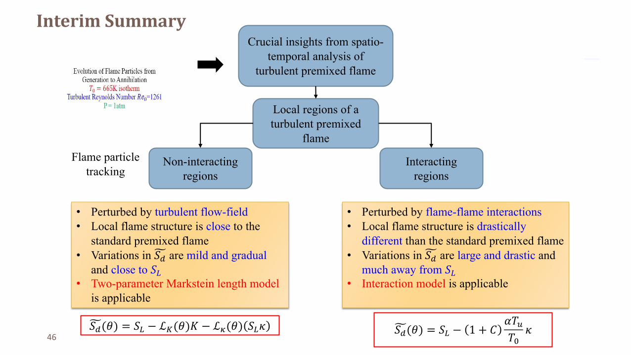
InterimSummary
46
Local regions of a turbulent premixed
flame
Non-interacting regions
Interactingregions
• Perturbed by turbulent flow-field• Local flame structure is close to the
standard premixed flame• Variations in �𝑆J are mild and gradual
and close to 𝑆"• Two-parameter Markstein length model
is applicable
�𝑆J(𝜃) = 𝑆" − ℒ�(𝜃)𝐾 − ℒ�(𝜃) 𝑆"𝜅
• Perturbed by flame-flame interactions• Local flame structure is drastically
different than the standard premixed flame• Variations in �𝑆J are large and drastic and
much away from 𝑆"• Interaction model is applicable
�𝑆J(𝜃) = 𝑆" − 1 + 𝐶𝛼𝑇<𝑇E
𝜅
Crucial insights from spatio-temporal analysis of
turbulent premixed flame
Flame particle tracking

Extremeturbulence:highKarlovitznumberflamepropagationandstructure

RegimeDiagrams
The regime diagram shown above is one example. Other regimediagrams also exist
𝐾𝑎8 = 1, 𝜂 = ℓ8
𝐾𝑎" = 1, 𝜂 = ℓ"
⁄ℓE ℓ"
Peters, N., 2001. Turbulent combustion.

HighKa-flamesinMichiganHi-Pilotburner
Skiba, A.W., Wabel, T.M., Carter, C.D., Hammack, S.D., Temme, J.E. and Driscoll, J.F., 2018, Combustion and Flame, 189, pp.407-432.Driscoll, J.F., Chen, J.H., Skiba, A.W., Carter, C.D., Hawkes, E.R. and Wang, H., 2020, Progress in Energy and Combustion Science, 76, p.100802.
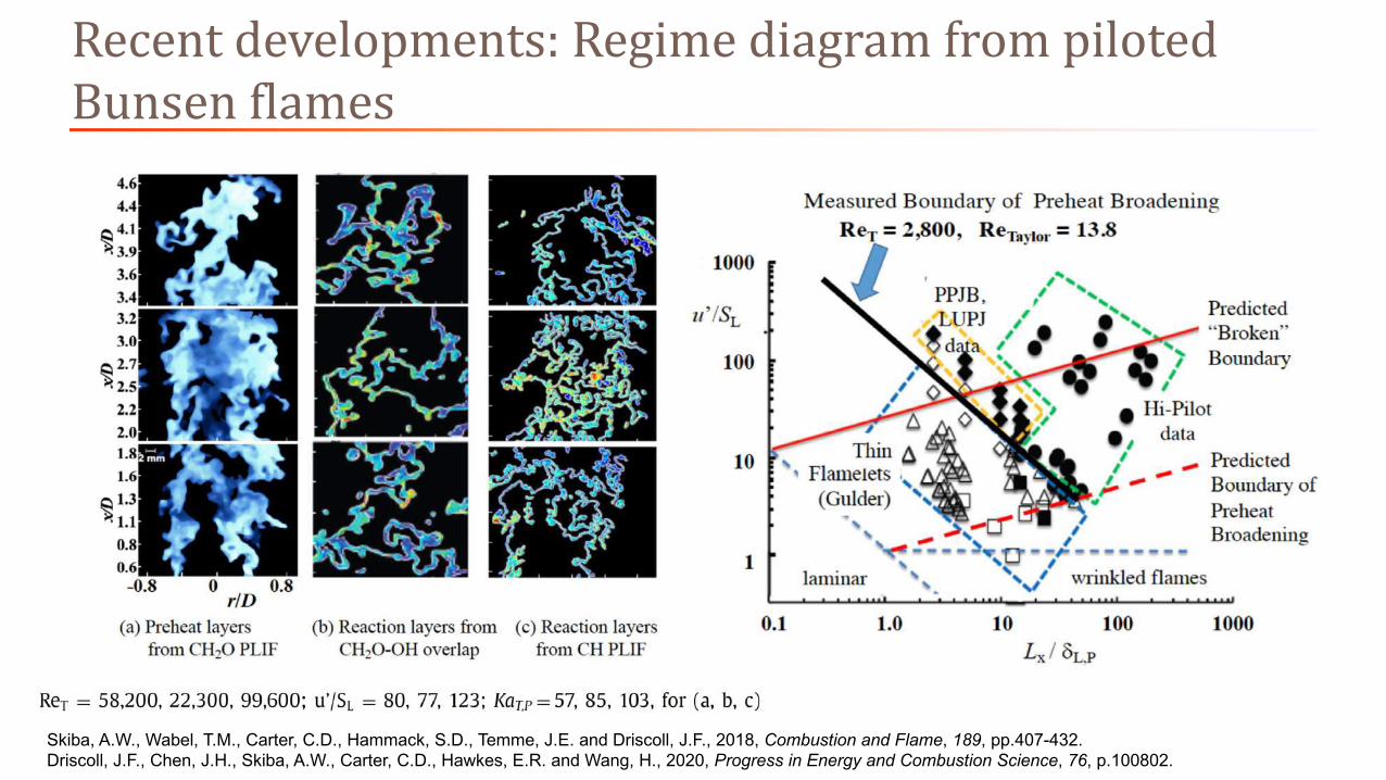
Recentdevelopments:RegimediagramfrompilotedBunsenflames
Skiba, A.W., Wabel, T.M., Carter, C.D., Hammack, S.D., Temme, J.E. and Driscoll, J.F., 2018, Combustion and Flame, 189, pp.407-432.Driscoll, J.F., Chen, J.H., Skiba, A.W., Carter, C.D., Hawkes, E.R. and Wang, H., 2020, Progress in Energy and Combustion Science, 76, p.100802.

HighKaflameDNS
Aspden A., Day, M., Bell J., 2019, Journal of Fluid Mechanics, 871, 1-21

Flame displacement speeds in intense turbulence
Yuvraj, Song, W., Dave, H.L., Im, H.G. and Chaudhuri, S., https://arxiv.org/abs/2106.08407

linear fit
Yuvraj, Song, W., Dave, H.L., Im, H.G. and Chaudhuri, S., https://arxiv.org/abs/2106.08407

Turbulent Flame Speed

55
Turbulent Premixed Flame

Turbulent Flame Speed
�� = −∫�¿ 𝜌 𝑣� Á Â𝑛 𝑑𝐴
∴ �� = ∫�¿ 𝜌 𝑆J Â𝑛 Á Â𝑛 𝑑𝐴
Defining
𝜌<𝑆n,gE𝐴 = ∫�¿,Ä�𝜌𝑆J𝑑𝐴
𝑆n,gE=A� ∫�¿,Ä�
�𝑆J𝑑𝐴
𝑣f = 𝑢 + 𝑆J &𝑛
∴ 𝑣�= 𝑢 − 𝑣f = −𝑆J &𝑛
Mass flow rate of premixed reactants into a flame surface

57
Damkohler (1940) discussed two limiting cases:• Wrinkled flamelet regime• Thin reaction zone regime
Turbulent flame propagation mode are fundamentallydifferent in the two limiting cases
When turbulence scales are larger than flame thickness,turbulence increases surface area
When turbulence scales are smaller than flame thickness,turbulence modifies the transport process
Turbulent Flame Speed

58
Wrinkled flamelet regime• 𝐴n is instantaneous flame area• 𝐴 is projected areaSince, mass-flux is constant �� = 𝜌<𝑆n𝐴 = 𝜌<𝑆"𝐴nThus, turbulence increases area 𝐴n > 𝐴 which causes 𝑆n > 𝑆" tothe leading order
Using simple geometric arguments it can be shown for weak turbulence𝑆n𝑆"= 1 +
𝑢13
𝑆"
(
Turbulent Flame Speed

59
.
Experiments: n Abdel-Gayed, R.G., Bradley, D. and Lawes, M., 1987. Turbulent burning velocities: a general correlation in terms of straining rates. Proceedings of the Royal Society of
London. A. Mathematical and Physical Sciences, 414(1847), pp.389-413.n Aldredge, R.C., Vaezi, V. and Ronney, P.D., 1998. Premixed-flame propagation in turbulent Taylor–Couette flow. Combustion and flame, 115(3), pp.395-405.n Kobayashi, H., Kawabata, Y. and Maruta, K., 1998, January. Experimental study on general correlation of turbulent burning velocity at high pressure. In Symposium
(International) on Combustion (Vol. 27, No. 1, pp. 941-948). Elsevier.n Kobayashi, H. and Kawazoe, H., 2000. Flame instability effects on the smallest wrinkling scale and burning velocity of high-pressure turbulent premixed flames. Proceedings
of the Combustion Institute, 28(1), pp.375-382.n Gülder, Ö.L., Smallwood, G.J., Wong, R., Snelling, D.R., Smith, R., Deschamps, B.M. and Sautet, J.C., 2000. Flame front surface characteristics in turbulent premixed
propane/air combustion. Combustion and Flame, 120(4), pp.407-416.
Theories/models/computations:n Clavin, P. and Williams, F.A., 1979. Theory of premixed-flame propagation in large-scale turbulence. Journal of fluid mechanics, 90(3), pp.589-604.n Anand, M.S. and Pope, S.B., 1987. Calculations of premixed turbulent flames by PDF methods. Combustion and Flame, 67(2), pp.127-142.n Yakhot, V., 1988. Propagation velocity of premixed turbulent flames. Combustion Science and Technology, 60(1-3), pp.191-214.n Kerstein, A.R. and Ashurst, W.T., 1992. Propagation rate of growing interfaces in stirred fluids. Physical review letters, 68(7), p.934.n Pocheau, A., 1994. Scale invariance in turbulent front propagation. Physical Review E, 49(2), p.1109.n Peters, N., 1999. The turbulent burning velocity for large-scale and small-scale turbulence. Journal of Fluid mechanics, 384, pp.107-132.n Lipatnikov A. N. and Chomiak J., 2002, Turbulent flame speed and thickness, Progress in Energy and Combustion Science, 78, 1-74n Poludnenko, A.Y. and Oran, E.S., 2011. The interaction of high-speed turbulence with flames: Turbulent flame speed. Combustion and flame, 158(2), pp.301-326.n Creta, F., Fogla, N. and Matalon, M., 2011. Turbulent propagation of premixed flames in the presence of Darrieus–Landau instability. Combustion Theory and
Modelling, 15(2), pp.267-298.n Chaudhuri S., Akkerman V., Law C. K. 20211, Spectral formulation of turbulent flame speed and consideration of hydrodynamic instability, Physical Review E, 84, 026322
(2011)
It is of interest to seek a solution:ST / SL = f (u’0 , SL , l0 , lL,...)
“… one of the most important unresolved problems in premixed turbulent combustion is determining the turbulent burning velocity”, Turbulent Combustion, Norbert Peters, Cambridge University Press, 2000.
Turbulent Flame Speed: literature
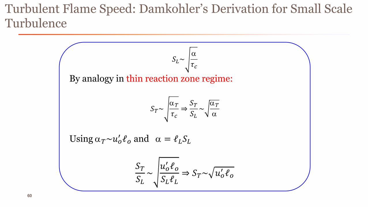
60
𝑆"~a𝜏g
By analogy in thin reaction zone regime:
𝑆n~an𝜏g⇒𝑆n𝑆"~
ana
Using an~𝑢13 ℓ1 and a = ℓ"𝑆"
𝑆n𝑆"~
𝑢13 ℓ1𝑆"ℓ"
⇒ 𝑆n~ 𝑢13 ℓ1
Turbulent Flame Speed: Damkohler’s Derivation for Small Scale Turbulence

Experiments
61

Turbulent Bunsen Flames
62 Kobayashi, H., Tamura, T., Maruta, K., Niioka, T. and Williams, F.A., 1996, January, Symposium (international) on combustion (Vol. 26, No. 1, pp. 389-396)

63 Kobayashi, H., Tamura, T., Maruta, K., Niioka, T. and Williams, F.A., 1996, January, Symposium (international) on combustion (Vol. 26, No. 1, pp. 389-396)
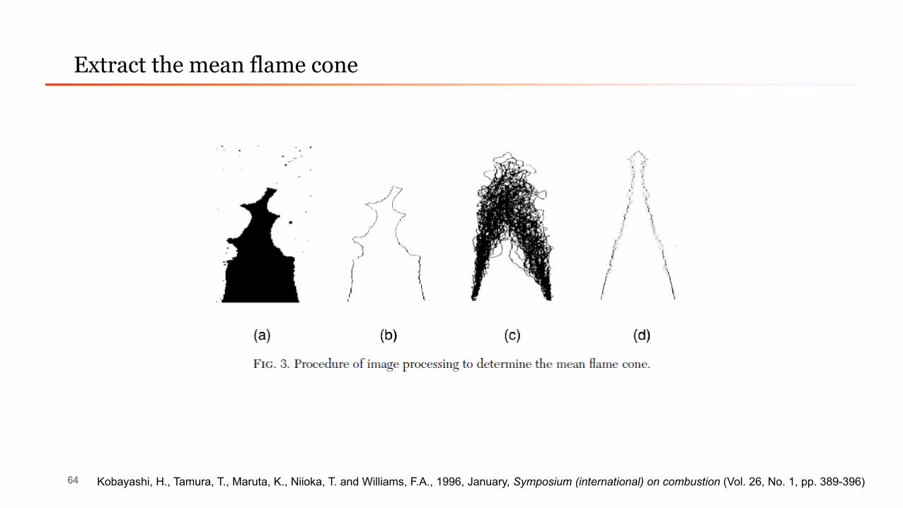
Extract the mean flame cone
64 Kobayashi, H., Tamura, T., Maruta, K., Niioka, T. and Williams, F.A., 1996, January, Symposium (international) on combustion (Vol. 26, No. 1, pp. 389-396)
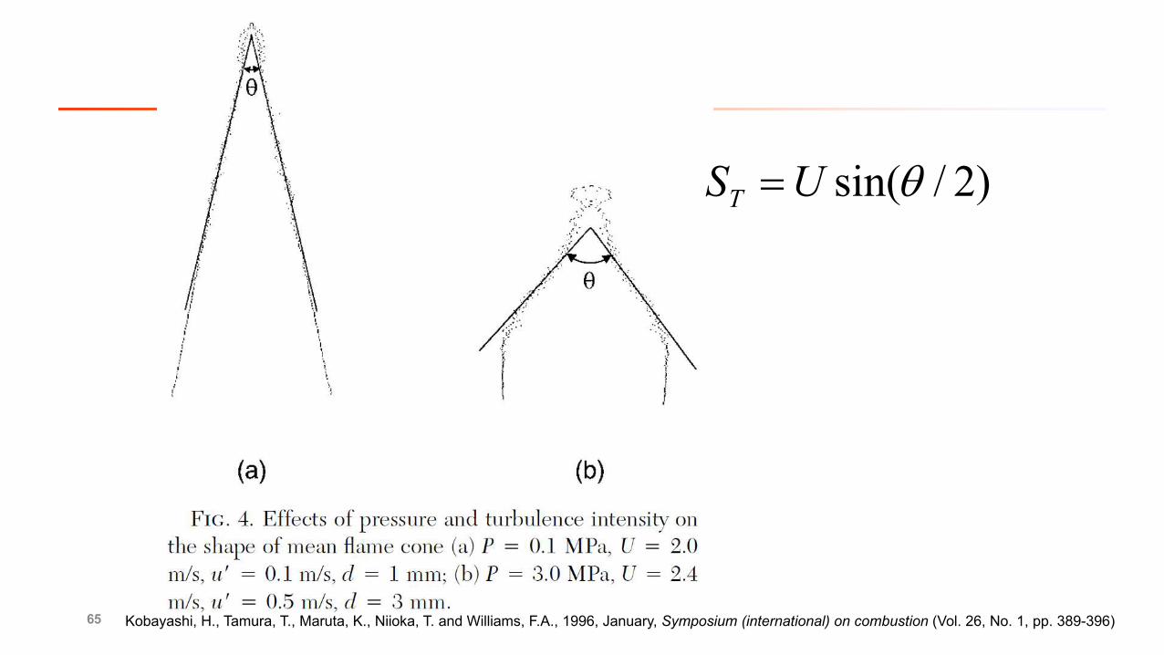
65
)2/sin(qUST =
Kobayashi, H., Tamura, T., Maruta, K., Niioka, T. and Williams, F.A., 1996, January, Symposium (international) on combustion (Vol. 26, No. 1, pp. 389-396)

Turbulent Flame Speed
66 Kobayashi, H., Tamura, T., Maruta, K., Niioka, T. and Williams, F.A., 1996, January, Symposium (international) on combustion (Vol. 26, No. 1, pp. 389-396)

Dual Chamber High Pressure Turbulent Combustion Vessel at Princeton
67

Experimental Setup
68
Dual-chamber design: Constant pressure (up to 25atm)Fan-generated nearly isotropic homogeneous turbulence
High speed Schlieren imaging
(b)

69

70
Emergence of Fine Scales with Pressure
CH4-air,(f=0.9, Le=1)
Chaudhuri, S., Wu, F., Zhu, D. and Law, C.K., 2012, Physical review letters, 108(4), p.044503.

71
High Speed Mie Images and Vector Fields
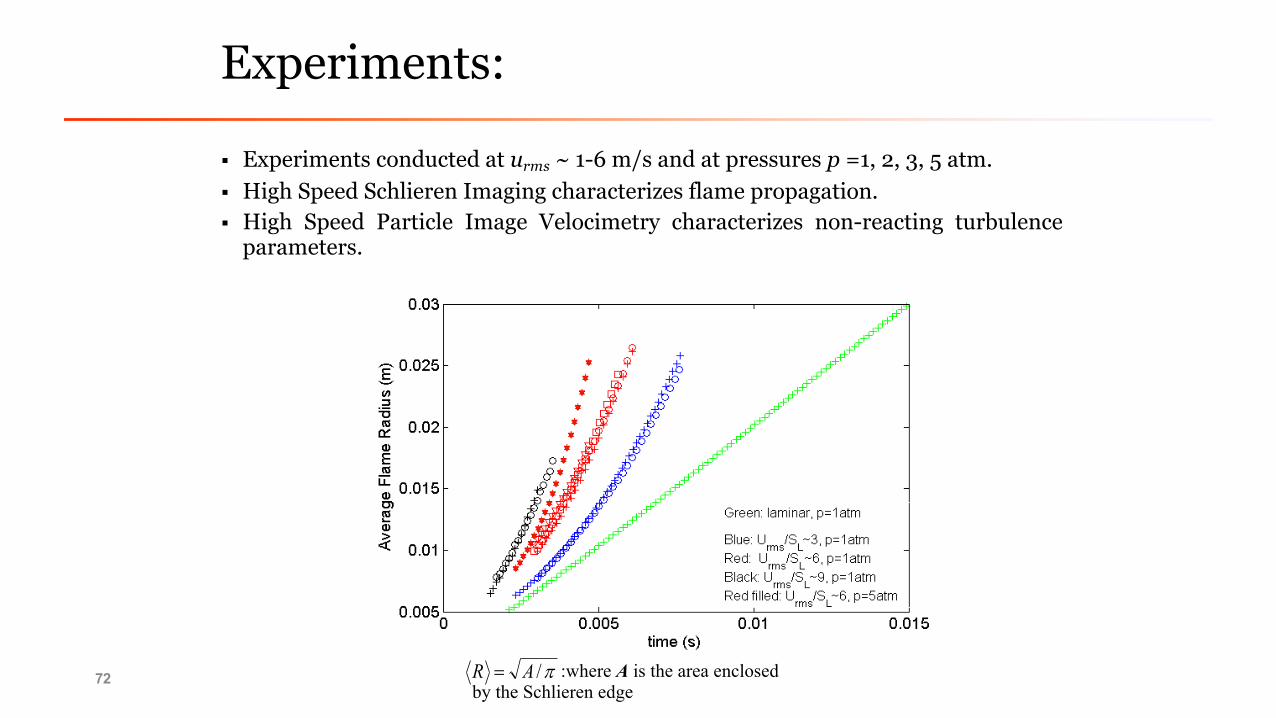
Experiments:
72
§ Experiments conducted at urms ~ 1-6 m/s and at pressures p =1, 2, 3, 5 atm.§ High Speed Schlieren Imaging characterizes flame propagation.§ High Speed Particle Image Velocimetry characterizes non-reacting turbulence
parameters.
p/AR = :where A is the area enclosed by the Schlieren edge
73
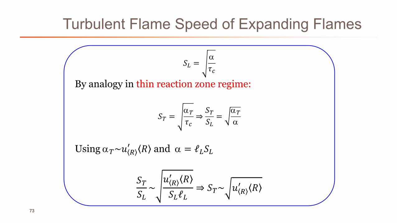
𝑆" =a𝜏g
By analogy in thin reaction zone regime:
𝑆n =an𝜏g⇒𝑆n𝑆"=
ana
Using an~𝑢 83 𝑅 and a = ℓ"𝑆"
𝑆n𝑆"~
𝑢 83 𝑅𝑆"ℓ"
⇒ 𝑆n~ 𝑢 83 𝑅
Turbulent Flame Speed of Expanding Flames

Turbulent Flame Propagation Rate
74 Chaudhuri, S., Wu, F., Zhu, D. and Law, C.K., 2012, Physical review letters, 108(4), p.044503.

Larger set: larger range of fuel, turbulence intensity

Scaling with Flame Thickness
76
Mk, Le increasing
0 ,1 / M bI R d= -
Symbols: C2H4-15% O2- 85% N2, f =1.3; CH4-air f =0.9, C2H4-air, f =1.3, n-C4H10-air, f =0.8 and C2H6O-air f=1.0 : Pressure 1-5atm. Lines: Leeds data (Lawes et. al. CNF 159, 2012) for the iso-C8H18 f =0.8-1.2 Pressure 1-10atm

Comprehensive ½-Power Scaling: Present (C0, C1,C2, C4) Fuels and Leeds C8 Data
77
0 ,1 / M bI R d= -Symbols: C2H4-15% O2- 85% N2, f =1.3; CH4-air f =0.9, C2H4-air, f =1.3, n-C4H10-air, f =0.8 and C2H6O-air f =1.0 : Pressure 1-5atm. Lines: Leeds data (Lawes et. al. CNF 159, 2012) for the iso-C8H18 f =0.8-1.2 Pressure 1-10atmChaudhuri, S., Wu, F. and Law, C.K., 2013, Physical Review E, 88(3), p.033005.

Turbulent Flame Speed: Surface Fitting
'/m n
eff
L L M
ud R dt RS S d
æ ö æ öµ ç ÷ ç ÷ç ÷ è øè ø
m = 0.43, n = 0.45 [≈ 0.5]
Chaudhuri, S., Wu, F. and Law, C.K., 2013, Physical Review E, 88(3), p.033005.

C4-C8 n-alkanes
Wu, F., Saha, A., Chaudhuri, S. and Law, C.K., 2015, Proceedings of the Combustion Institute, 35(2), pp.1501-1508.

Scaling for C4-C8 n-alkanes
Wu, F., Saha, A., Chaudhuri, S. and Law, C.K., 2015, Proceedings of the Combustion Institute, 35(2), pp.1501-1508.

CH4-air data from National Central University, Taiwan
Jiang, L.J., Shy, S.S., Li, W.Y., Huang, H.M. and Nguyen, M.T., 2016, Combustion and Flame, 172, pp.173-182.

H2 blend – air data from Xian Jiaotong University, China
Cai, X., Wang, J., Bian, Z., Zhao, H., Zhang, M. and Huang, Z., 2020, Combustion and Flame, 212, pp.1-12.Zhao, H., Wang, J., Cai, X., Dai, H., Bian, Z. and Huang, Z., 2021, International Journal of Hydrogen Energy.

Data from Georgia Tech, USA
Fries D., Ochs B. A., Saha A., Ranjan D., Menon S. Combustion and Flame 199 (2019), 1-13

Experiments on Instability Turbulence Interaction
84
Laminar Flame with Cellular Instability Turbulent Flame
Cellular instability:• Increase the surface area
• Flame acceleration
Turbulence:• Wrinkle the surface & enhanced mixing
• Flame acceleration

Methodology
85
Cellular instability
Turbulence
Flame acceleration due to cellular instability (𝐿𝑒 =
1 and 𝐿𝑒 < 1)
Flame acceleration due to turbulence
Scaling analysis (𝐿𝑒 = 1)
Experimental investigation (𝐿𝑒 = 1 and 𝐿𝑒 < 1)
Identify conditions

( ) ( ) 1/21/2, 0 0Re /T f rms L LU R S dé ù= ë û
Propagation of Turbulent Flames
1/2,ReT f
Turbulent flame speed scaling[1]-[4]
In our case,
So, in turbulent flame propagation
𝑆n~ ⁄[ 𝑅 𝛿"]𝛽n = 𝑃𝑒É¿, 𝛽n≈ 0.67
𝑆n~𝑅𝑒n,fA/(
𝑅𝑒n,f = ⁄𝑈�c� 𝑅 𝑆"𝛿"
𝑈�c� ∝ 𝑅 E.::
[3] Wu, F., Saha, A., Chaudhuri, S. and Law, C. K., 2015. Proceedings of the Combustion Institute, 35(2), 1501-1508.
[1] Chaudhuri, S., Wu, F. and Law, C. K., 2013. Physical Review E, 88(3), 033005.
[4] Jiang, L. J., Shy, S. S., Li, W. Y., Huang, H. M. and Nguyen, M. T., 2016. Combustion and Flame, 172, 173-182.
[2] Saha, A., Chaudhuri, S. and Law, C. K., 2014. Physics of Fluids, 26(4), 045109.

Experimental Setup
87
Dual-chamber design: Constant pressure (up to 25atm)Fan-generated nearly isotropic homogeneous turbulence
High speed Schlieren imaging
(b)

0/ LPe R d=
Propagation of Laminar Cellular Flames (𝐿𝑒 = 1)
88
è Three-stage behavior[1]
§ Smooth expansion§ Transition§ Saturation
𝑆",®~𝑃𝑒ÉÄ, 𝛽g ≈ 0.3
slope=0.3
⁄H( ⁄O( N( , 𝜙 = 1, T = 2400K (𝐿𝑒 ≈ 1)
acceleration exponent
𝑆 ",®=
⁄𝑆 ",®𝑆 "E
DL instability
[1] Yang, S., Saha, A., Wu, F. and Law, C.K., 2016, Combustion and Flame, 171, pp.112-118.

Propagation of Laminar Cellular Flames (𝐿𝑒 < 1)
§ For 𝐿𝑒 < 1, diffusional-thermal instability also appears
𝑆",®~𝑃𝑒ÉÄ, 𝛽g ≈ 0.33
• Three-stage behavior still exists
Le
• The smaller the Le, the larger the 𝑆",®
• In saturation stage,
⁄H( ⁄O( ⁄He Ar , 𝜙 = 0.4, T = 2110K
Liu Z., Yang S., Law C.K., Saha A. Proceedings of the Combustion Institute 37 (2) (2019), 2611-2618

Acceleration Exponent
90
Laminar flame with Cellular instability
Turbulent cellularly-stable flame
𝑆",®~𝑃𝑒E.: 𝑆n~𝑃𝑒E.ÕÖ

Turbulence-DLInstabilityInteraction

Turbulence-InstabilityInteraction
DL growth rate
Turbulent eddy frequency
Conjecture: DL instability develops in turbulence if
𝜎×"(Ø) >> 𝜔±<�®
(Ø)
𝜎×"Ø = 𝛸 𝛩 𝑆"𝑘 1 − ⁄𝑘 𝑘g
𝛸 𝛩 =𝛩
𝛩 + 1 𝛩 + 1 − 𝛩9A ⁄A ( − 1
𝑘g𝑙" = ℎ® +3𝛩 − 1𝛩 − 1 𝑀𝑘 −
2𝛩𝛩 − 1
�A
Þ ℎ 𝜗𝜗 𝑑𝜗 + 2𝑃𝑟−1 ℎ® −
∫AÞ ℎ 𝜗 𝑑𝜗𝛩 − 1
9A𝜏±<�®Ø =
𝑢 Ø(
𝜀=
𝑙0𝑢30
𝑘𝑘𝟎
9 ⁄( :
𝜏±<�®Ø = 2 ⁄𝜋 𝜔±<�®
Ø
Chaudhuri, S., Akkerman, V.Y. and Law, C.K., 2011, Physical Review E, 84(2), p.026322.

Turbulence-DLInstabilityRegimeDiagram
𝛽 = 𝑚𝑖𝑛∀ØäØ𝟎
𝜔±<�®Ø
𝜎×"Ø
Þ 𝛽 = 𝑚𝑖𝑛ØÄäØäØ𝟎
åæçèé@?
Ø𝟎Ø
⁄A :1 − Ø
ØÄ
9A
𝑙E/𝑙"Chaudhuri, S., Akkerman, V.Y. and Law, C.K., 2011, Physical Review E, 84(2), p.026322.
𝑈 ./0/𝑆 12
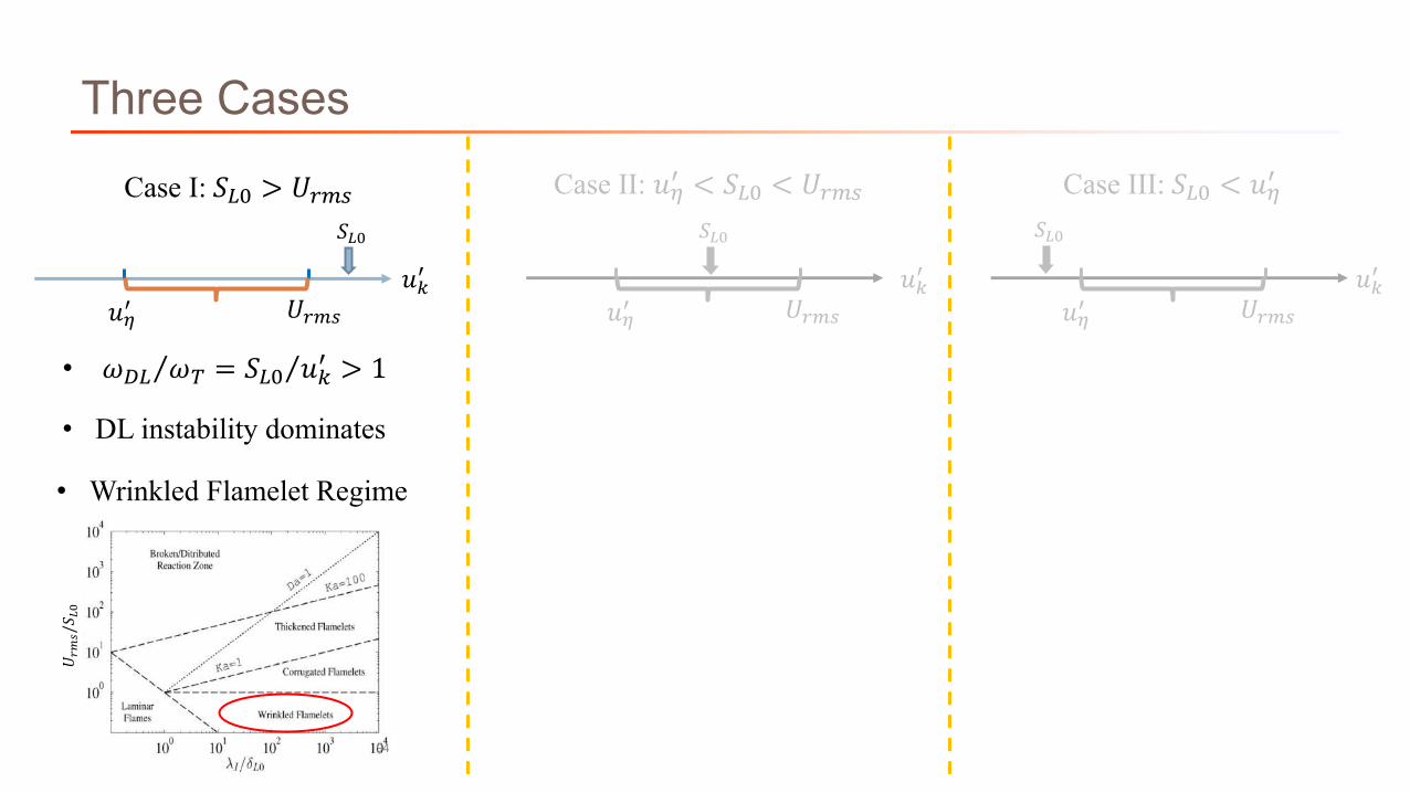
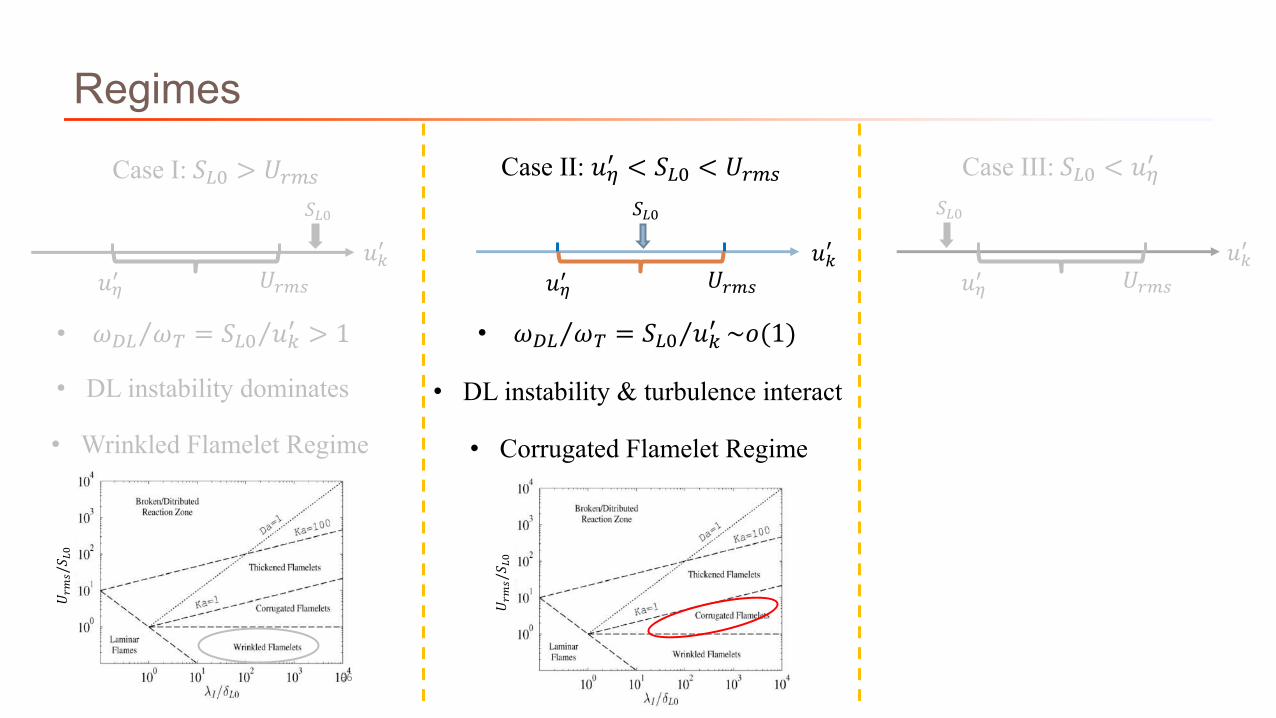
Three Cases
94
Case I: 𝑆"E > 𝑈�c� Case II: 𝑢63 < 𝑆"E < 𝑈�c� Case III: 𝑆"E < 𝑢63
𝑆*+ 𝑆*+
• ⁄𝜔×" 𝜔n = ⁄𝑆"E 𝑢Ø3 > 1
• DL instability dominates
• Wrinkled Flamelet Regime
𝑢Ø3𝑈�c�𝑢63
𝑢Ø3𝑈�c�𝑢63
𝑆*+
𝑢Ø3𝑈�c�𝑢63

Case I: 𝑆12 > 𝑈./0
95
⁄H( ⁄O( N( , 𝜙 = 1, T = 2400K, P = 1 − 10atm
𝐿𝑒 = 1 𝐿𝑒 < 1Saturation stage of DL
instabilityTurbulent cellularly-
stable flame
• Acceleration exponent is close to the saturation stage of DL instability
Darrieus-Landau instability dominates the flame
propagation in Wrinkled Flamelet Regime!
Le
⁄H( ⁄O( ⁄He Ar , 𝜙 = 0.4, T = 2110K, P = 1atm
The acceleration exponent is independent of Le, but 𝑆n decreases
with Le.
• Cellular instability dominates in this regime for 𝐿𝑒 < 1
𝑈 ./0/𝑆 12
Regimes
96
Case I: 𝑆"E > 𝑈�c� Case II: 𝑢63 < 𝑆"E < 𝑈�c� Case III: 𝑆"E < 𝑢63
𝑆*+
• ⁄𝜔×" 𝜔n = ⁄𝑆"E 𝑢Ø3 > 1 • ⁄𝜔×" 𝜔n = ⁄𝑆"E 𝑢Ø3 ~𝑜(1)
• DL instability dominates • DL instability & turbulence interact
• Wrinkled Flamelet Regime • Corrugated Flamelet Regime
𝑈 ./0/𝑆 12
𝑆*+
𝑢Ø3𝑈�c�𝑢63
𝑆*+
𝑢Ø3𝑈�c�𝑢63
𝑢Ø3𝑈�c�𝑢63

Le
• Acceleration exponent is between the saturation stage of DL instability and the turbulent cellularly-stable flame
⁄H( ⁄O( N( , 𝜙 = 1, T = 1800K, P = 1 − 10atm
Case II: 𝑈./0 > 𝑆1,2 > 𝑢67
97
𝐿𝑒 = 1 𝐿𝑒 < 1Saturation stage of DL
instabilityTurbulent cellularly-
stable flame
⁄H( ⁄O( ⁄He Ar , 𝜙 = 0.4, T = 2110K, P = 1atm
The acceleration exponent is independent of Le, but 𝑆n decreases
with Le.
• Cellular instability and turbulence interact in this regime for 𝐿𝑒 < 1
Darrieus-Landau instability and turbulence both contribute
to flame propagation in Corrugated Flamelet Regime!

Regimes
98
Case II: 𝑢63 < 𝑆"E < 𝑈�c� Case III: 𝑆"E < 𝑢63
ku ¢uh¢ rmsU
𝑆*+
• ⁄𝜔×" 𝜔n = ⁄𝑆"E 𝑢Ø3 ~𝑜(1) • ⁄𝜔×" 𝜔n = ⁄𝑆"E 𝑢Ø3 < 1
• DL instability & turbulence interact • Turbulence dominates
• Corrugated Flamelet Regime • Thickened Flamelet Regime
𝑈 ./0/𝑆 12
𝑈 ./0/𝑆 12
𝑈 ./0/𝑆 12
Case I: 𝑆"E > 𝑈�c�
• ⁄𝜔×" 𝜔n = ⁄𝑆"E 𝑢Ø3 > 1
• DL instability dominates
• Wrinkled Flamelet Regime
𝑆*+
𝑢Ø3𝑈�c�𝑢63
𝑆*+
𝑢Ø3𝑈�c�𝑢63
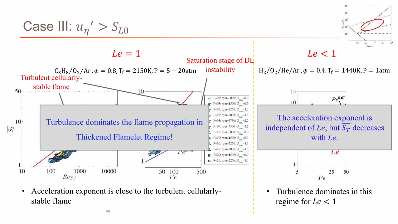
⁄H( ⁄O( ⁄He Ar , 𝜙 = 0.4, T = 1440K, P = 1atm
• Acceleration exponent is close to the turbulent cellularly-stable flame
⁄C:Hð ⁄O( Ar , 𝜙 = 0.8, T = 2150K, P = 5 − 20atm
Le
Case III: 𝑢67 > 𝑆12
99
𝐿𝑒 = 1 𝐿𝑒 < 1Saturation stage of DL
instabilityTurbulent cellularly-
stable flame
The acceleration exponent is independent of Le, but 𝑆n decreases
with Le.
• Turbulence dominates in this regime for 𝐿𝑒 < 1
Turbulence dominates the flame propagation in
Thickened Flamelet Regime!

InstabilityTurbulenceInteraction

Summary
§ Darrieus-Landau instability in turbulent flames:
§ revised regime diagram
§ Diffusional-thermal instability in turbulent flames:§ Influences the total burning rate, but does not influence the
acceleration exponent.
(with respect to DL instability)
Chaudhuri, S., Akkerman, V.Y. and Law, C.K., 2011, Physical Review E, 84(2), p.026322.

Blowoff
102

Characteristics of flows separated by bluff bodies:Non-reacting flows
S Chaudhuri, PhD Thesis 2010

Characteristics of flows separated by bluff bodies:Reacting flows
S Chaudhuri, PhD Thesis 2010

Early views on blowoff§ Longwell (1953) suggested: blowoff due to imbalance in rate of
reactions in RZ
§ Insufficient heat supply by RZ to fresh gases (Williams GC, HottelH. et al. 1951)
§ Insufficient contact time of the fresh mixture in the shear layer with the burnt product in RZ. (Zukoski 1954)
§ Blowoff is preceded by two distinct stages of flame hole formation (Nair and Lieuwen, 2007)
§ But these studies did not connect the early stages of blowoff dynamics with the final blowoff event and a complete mechanism was lacking.
105

Effects of exothermicity
Results indicate substantially reduced turbulence intensities and vorticity magnitudes in combusting flows relative to the non-reacting flow for e.g. by Soteriou, Ghoniem (1994).
Fureby and Lofstrom (1994): vorticity field strength was much weaker and ‘‘less structured’’ (1994) in the presence of combustion.
Fuji and Eguchi (1981) and Bill and Tarabanis (1986) noted that turbulence levels in the reacting flow were much lower than the non-reacting case, particularly inthe vicinity of the recirculation zone boundary.
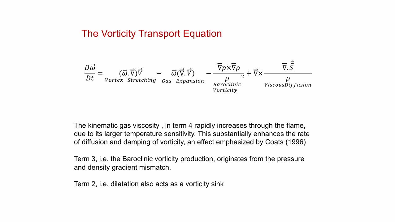
𝐷𝜔𝐷𝑡 = (𝜔. ∇)𝑉
ó1�±�^ @±��±gôeõ½− 𝜔(∇. 𝑉)öd� ÷^§dõ�e1õ
−∇𝑝×∇𝜌𝜌
ød�1gùeõegó1�±ege±_
( + ∇×∇. 𝑆𝜌
óe�g1<�×eff<�e1õ
The kinematic gas viscosity , in term 4 rapidly increases through the flame, due to its larger temperature sensitivity. This substantially enhances the rate of diffusion and damping of vorticity, an effect emphasized by Coats (1996)
Term 3, i.e. the Baroclinic vorticity production, originates from the pressure and density gradient mismatch.
Term 2, i.e. dilatation also acts as a vorticity sink
The Vorticity Transport Equation

Near Blowoff Dynamics in Bluff Body Stabilized Flames
• Many researchers observed that near blowoff flames are highly unsteady and unstable (Zukoski (1958), Williams (1966) H.M. Nicholson (1948))
• Nicholson and Field (1948) described large scale pulsations in rich bluff body flames as they were blowing off.
• Observations of large scale, sinuous oscillations of a flame near blowoff were presented by Thurston (1958).
• Hertzberg et al. (1991) measured velocity fluctuations in a bluff body wake, indicating a growing amplitude of a relatively narrowband oscillation as blowoff was approached that they attributed to vortex shedding.
• A number of more recent studies by Nair and Lieuwen (2007), Kiel et al. (2007) and Erickson et al. have also noted these dynamics (2007).

Early views on blowoff
• Longwell (1953) suggested: blowoff due to imbalance in rate of entrainment of reactants (a PSR RZ)
• Insufficient heat supply by RZ to fresh gases (Williams GC, Hottel H. et al. 1951)• Insufficient contact time of the fresh mixture in the shear layer with the burnt
product in RZ. (Zukoski 1954)• Extinction of a strained flamelet (Yamaguchi 1985)• But these studies did not connect the early stages of blowoff dynamics with the final
blowoff event as complete mechanism was lacking.

Blowoff Correlation
S. Shanbhogue, S. Hussain and T. Lieuwen, Progress in Energy and Combustion Dynamics, 2009

Stage 1:
Initiation of flame hole, its convection downstream and healing. However the flamecan persist indefinitely at this stage. This local extinction is hypothesized to be occurring at points where klocal > kextinct
S. Nair and T. Lieuwen, Journal of Propulsion and Power 2007
Two stages of blowoff
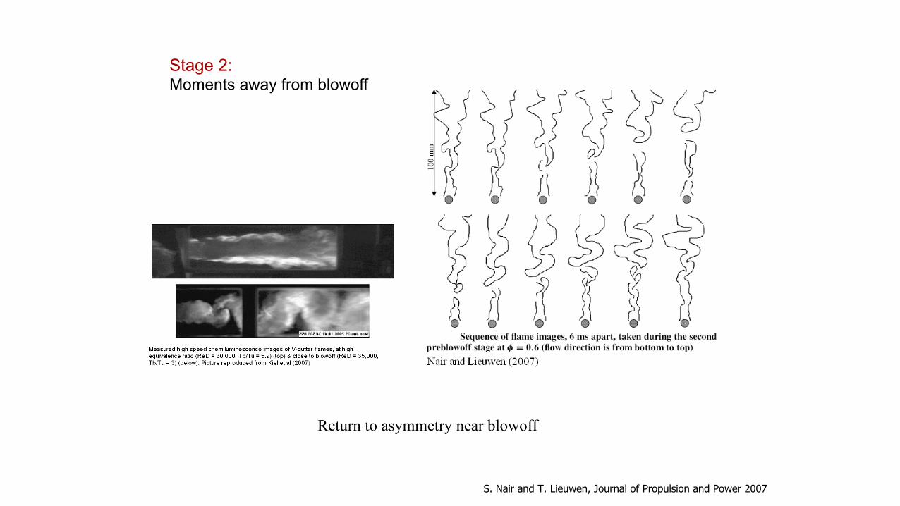
Stage 2:Moments away from blowoff
Return to asymmetry near blowoff
S. Nair and T. Lieuwen, Journal of Propulsion and Power 2007

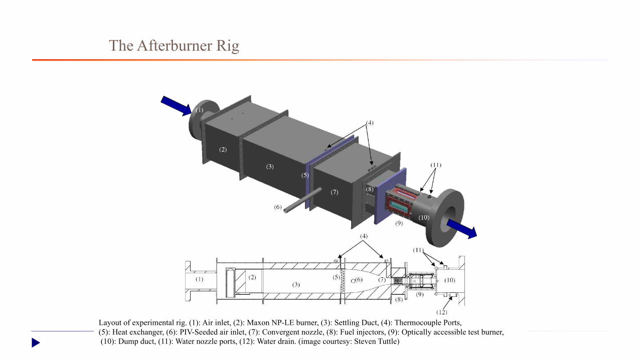
The Afterburner Rig
Layout of experimental rig. (1): Air inlet, (2): Maxon NP-LE burner, (3): Settling Duct, (4): Thermocouple Ports, (5): Heat exchanger, (6): PIV-Seeded air inlet, (7): Convergent nozzle, (8): Fuel injectors, (9): Optically accessible test burner,(10): Dump duct, (11): Water nozzle ports, (12): Water drain. (image courtesy: Steven Tuttle)

PIV CameraPIV Laser 532nm
Experimental Setup
PMT HS Camera
OL
OLFImaging setup
Simultaneous PIV PLIF setup
115

Stable Flame at f = 0.85
High speed chemiluminescence emission images for a stable flame very far from blowoff for Um = 18.3 m/s at f = 0.85 at 500 frames per second and 100 µs exposure.
Extinction reignition and blowoff : movie
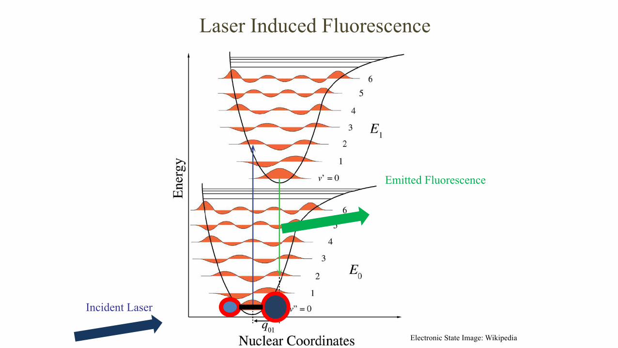
Laser Induced Fluorescence
Incident Laser
Emitted Fluorescence
Electronic State Image: Wikipedia

Particle Image Velocimetry
Raffell, Willert, Wereley, Kompenhans: Particle Image Velocimetry, Springer
Ds
Dt119
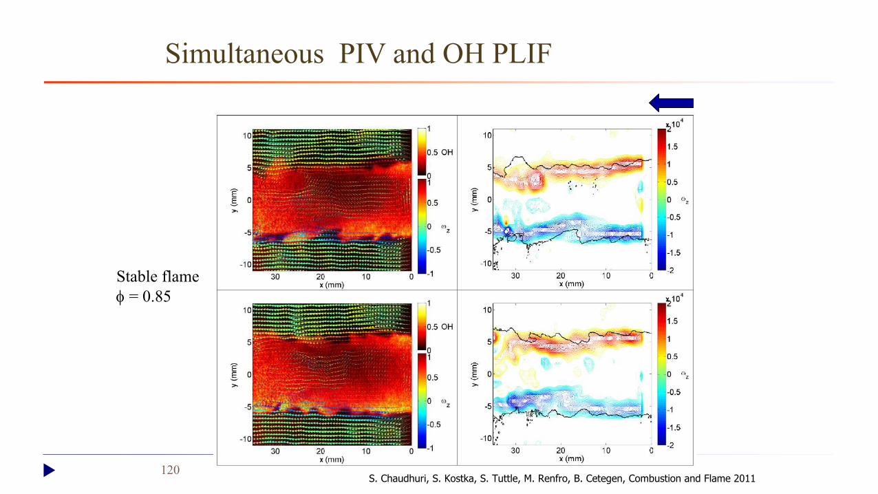
Simultaneous PIV and OH PLIF
Stable flamef = 0.85
S. Chaudhuri, S. Kostka, S. Tuttle, M. Renfro, B. Cetegen, Combustion and Flame 2011120

Near blowoffflamef = 0.60
Extinction along shear layers and recirculation zone burn
121
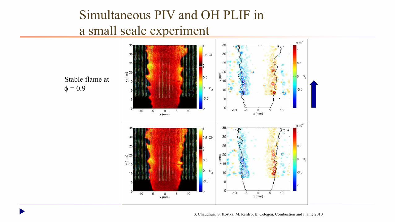
Simultaneous PIV and OH PLIF in a small scale experiment
Stable flame at f = 0.9
S. Chaudhuri, S. Kostka, M. Renfro, B. Cetegen, Combustion and Flame 2010
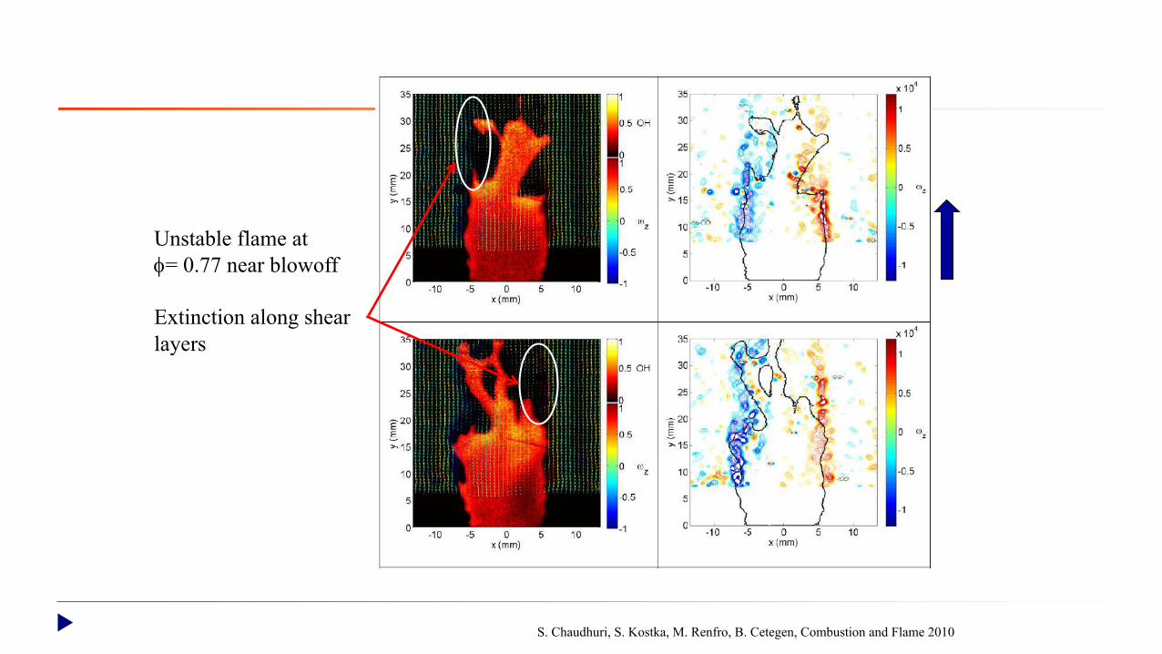
Unstable flame at f= 0.77 near blowoff
Extinction along shearlayers
S. Chaudhuri, S. Kostka, M. Renfro, B. Cetegen, Combustion and Flame 2010

Mean Uy and wz superimposed with OH-PLIF
f = 0.90 : Far from blowoff f = 0.77 : Near blowoff
-30 -20 -10 0 10 20 30-10
-5
0
5
10
15
20
x (mm)
Uy (m
/s)
0
0.1
0.2
0.3
0.4
0.5
0.6
OH
PLI
F
Axial Location y = 20 mm
-30 -20 -10 0 10 20 30-1
-0.5
0
0.5
1x 10⁴
x (mm)
wz (1
/s)
0
0.1
0.2
0.3
0.4
0.5
0.6
OH
PLI
F
Axial Location y = 20 mm
-30 -20 -10 0 10 20 30-10
-5
0
5
10
15
20
x (mm)
Uy (m
/s)
0
0.1
0.2
0.3
0.4
0.5
0.6
OH
PLI
F
Axial Location y = 20 mm
-30 -20 -10 0 10 20 30-1
-0.5
0
0.5
1x 10⁴
x (mm)
wz (1
/s)
0
0.1
0.2
0.3
0.4
0.5
0.6
OH
PLI
F
Axial Location y = 20 mm
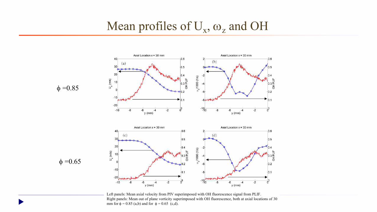
Mean profiles of Ux, wz and OH
f =0.85
f =0.65
Left panels: Mean axial velocity from PIV superimposed with OH fluorescence signal from PLIF.Right panels: Mean out of plane vorticity superimposed with OH fluorescence, both at axial locations of 30mm for f = 0.85 (a,b) and for f = 0.65 (c,d).

Basics of Premixed Flame Extinction
1. Extinction by volumetric heat loss2. Extinction by stretch
a. Le > 1b. Le < 1
Peters Summer school lecture notes 2010
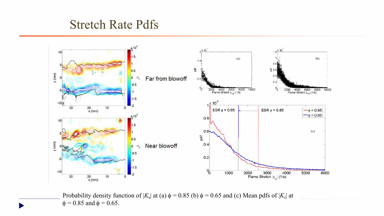
Probability density function of |Ks| at (a) f = 0.85 (b) f = 0.65 and (c) Mean pdfs of |Ks| at f = 0.85 and f = 0.65.
Stretch Rate Pdfs

Proposed blowoff mechanism
Towards blowoff f ¯ and hence SL¯ , so flame shifts from outside towards the shear layer vortices. Partial flame extinction along shear layers due to kflame > kextinction by convecting vortices.
Non reacting unburnt mixture entrains into RZand due to favorable flow time scales reacts within RZ . Hence OH and chemiluminescence
Reacting RZ reignites the shear layers to cause reignition
Reacting RZ fails to reignite the shear layers
More parts of the shear layers become “cold” Absolute instability : Asymmetric mode steps in to cause greater perturbations
Blowoff
S. Chaudhuri, S. Kostka, M. Renfro, B. Cetegen, Combustion and Flame 2010128

Works at Cambridge: lean CH4-air flames
J. Kariuki, J. Dawson and E. Mastorakos, Combustion and Flame 2012
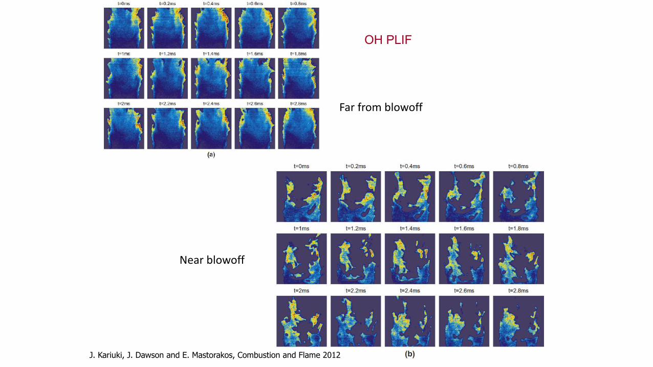
Far from blowoff
Near blowoff
J. Kariuki, J. Dawson and E. Mastorakos, Combustion and Flame 2012
OH PLIF

Blowoff in Vitiated Flows
Vitiated
Unvitiated
S. Tuttle, S. Chaudhuri, S. Kostka, K. Vaughn, T. Jensen, M. Renfro, B. Cetegen, Combustion and Flame 2012

PIV–PLIF of near blowoff vitiated flames
Significant difference between vitiated and unvitiated blowoff

Flame images obtained by reversing the Mie scattering images obtained during the PIV experiments for the 10-mm-diameter disk-shaped bluff-body flame holder (arrows show the length scale l = Um/f ). (.The values in black represent the ratio of the length of recirculation zone to l.
Forced blowoff mechanism
A. Chapparo, B.M. Cetegen, Combustion and Flame 2006
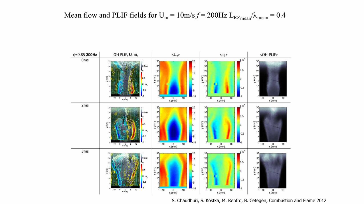
Mean flow and PLIF fields for Um = 10m/s f = 200Hz LRZmean/lmean = 0.4
S. Chaudhuri, S. Kostka, M. Renfro, B. Cetegen, Combustion and Flame 2012

Forced Blowoff : Forced Vortex Shedding
Forced Blowoff Unforced Blowoff
S. Chaudhuri, S. Kostka, M. Renfro, B. Cetegen, Combustion and Flame 2012

Blowoff in Swirl Stabilized Flames (Ga.Tech)
T. M. Muruganandam, S. Nair, D. Scarborough, Y. Neumeier, J. Jagoda, T. Lieuwen, J. Seitzman , B. Zinn, Journal of Propulsion and Power, 2005

Blowoff in Swirl Stabilized Flames (DLR)
Experimental Setup
Time averaged OH* and streamlines
M. Stoehr, I. Box, C. Carter, W. Meier, Proceedings of the Combustion Institute 2011

Consecutive images with PIV-PLIF near blowoff
Enlarged views
Final blowoff
Near and Final Blowoff

139
Thank you!

A. Kerstein, W. Ashurst and F. A. Williams Physical Review A (1988), S. Chaudhuri, V. Akkerman, C.K. Law, Physical Review E, (2011)
G equation: GSGtG
d Ñ=Ñ×+¶¶ V
0 ;0),,,(),,,( ==+= g(x,y,z,t tzyxgztzyxG
For a statistically planar and steady flame in isotropic turbulence, setting:
Turbulent Flame Speed: Analytical Derivation
G(x,y,z,t)=0
LS~
GSS LT Ñ=/0, 21
0'01~ ú
û
ùêë
é÷÷ø
öççè
æ÷÷ø
öççè
æ
LLL
T
ll
Su
MkSS
𝑆J = 𝑆" − 𝑆"𝑙c𝐾 − 𝑙c𝑎n

Computational Details BFPT Algorithm: Estimation Stage
Flame particle’s equation𝑑𝒙N
𝑑𝑡 = 𝒗N = 𝒖N + 𝑆JN𝒏N
During backtracking, the discretized eq. is implicit[1,2]
𝒙N 𝑡 − Δ𝑡 = 𝒙N 𝑡 + −𝒗N 𝑡 − Δ𝑡 Δ𝑡
BFPT Algorithm
Estimation Stage Correlation Stage
During estimation, 𝑣N 𝑡 − Δ𝑡 ≈ 𝑣N(𝑡)𝒙N 𝑡 − Δ𝑡 = 𝒙N 𝑡 + −𝒗N 𝑡 Δ𝑡
Estimation Stage
[1] A. Nahum and A. Seifert, Phys. Rev. E, 74 (2006) 016701.[2] H. L. Dave, A. Mohan, S. Chaudhuri, Combust. Flame. 196 (2018) 386-399

Computational Details BFPT Algorithm: Correlation Stage
142
DNS of statistically planar flames
Snapshots of DNS saved at fine time
interval
Snapshots are fed to the BFPT algorithm
in reverse order
Source location of turbulent flame
surfaces
𝐷e =𝑨e. 𝑩e
max{ 𝑨e 𝑩e }(• 𝑨e - “available” velocity vector• 𝑩e - “required” velocity vector
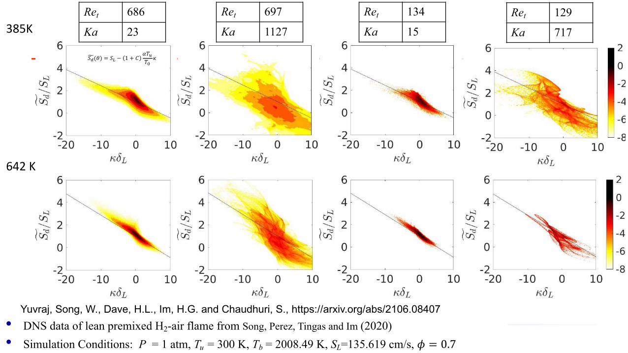
385K
642 K
Ret 686
Ka 23
Ret 697
Ka 1127
Ret 134
Ka 15Ret 129
Ka 717
• DNS data of lean premixed H2-air flame from Song, Perez, Tingas and Im (2020)• Simulation Conditions: P = 1 atm, Tu = 300 K, Tb = 2008.49 K, SL=135.619 cm/s, 𝜙 = 0.7
8𝑆9(𝜃) = 𝑆1 − 1 + 𝐶𝛼𝑇@𝑇2
𝜅
Yuvraj, Song, W., Dave, H.L., Im, H.G. and Chaudhuri, S., https://arxiv.org/abs/2106.08407