Structural Models of Corporate Bond Pricing: An Empirical - testing

Structural Models of Corporate Bond Pricing:

An Empirical Analysis

Young Ho Eom

Yonsei University

Jean Helwege

University of Arizona

Jing-Zhi Huang

Penn State University

This article empirically tests five structural models of corporate bond pricing: those

of Merton (1974), Geske (1977), Longstaff and Schwartz (1995), Leland and Toft

(1996), and Collin-Dufresne and Goldstein (2001). We implement the models using a

sample of 182 bond prices from firms with simple capital structures during the period

1986–1997. The conventional wisdom is that structural models do not generate

spreads as high as those seen in the bond market, and true to expectations, we find

that the predicted spreads in our implementation of the Merton model are too low.

However, most of the other structural models predict spreads that are too high on

average. Nevertheless, accuracy is a problem, as the newer models tend to severely

overstate the credit risk of firms with high leverage or volatility and yet suffer from a

spread underprediction problem with safer bonds. The Leland and Toft model is an

exception in that it overpredicts spreads on most bonds, particularly those with high

coupons. More accurate structural models must avoid features that increase the credit

risk on the riskier bonds while scarcely affecting the spreads of the safest bonds.

The seminal work of Black and Scholes (1973) and Merton (1974) in the

area of corporate bond pricing has spawned an enormous theoretical

literature on risky debt pricing. One motivating factor for this burgeoning

literature is the perception that the Merton model cannot generate

sufficiently high-yield spreads to match those observed in the market.

Thus the recent theoretical literature includes a variety of extensions and

We are grateful to an anonymous referee and especially Ken Singleton and Maureen O’Hara (the editors)for detailed and helpful comments and suggestions. We also thank Edward Altman, Pierluigi Balduzzi,Brian Barrett, Pierre Collin-Dufresne, Bob Goldstein, Spencer Martin, and seminar participants at theUniversity of Houston, Korea University, Ohio State University, Seoul National University, the Bank forInternational Settlements, FDIC, the Federal Reserve Bank of Cleveland, the 2001 Western FinanceAssociation meetings, the 2001 Financial Management Association meetings, Cornell’s 12th AnnualDerivatives Conference, and the 2002 European Finance Association meetings for helpful commentsand suggestions. Thanks also to Niki Boyson and Doug Clark for excellent assistance in the constructionof the data. Y.H. Eom acknowledges a research grant from the Yonsei Business Research Institute.J.-Z. Huang acknowledges a summer grant from the Smeal College of Business for partial support.Address correspondence to Jing-Zhi Huang, Smeal College of Business, Penn State University, UniversityPark, PA 16802, or e-mail: [email protected].

The Review of Financial Studies Vol. 17, No. 2, pp. 499–544 DOI: 10.1093/rfs/hhg053

ª 2004 The Society for Financial Studies; all rights reserved.

improvements, such as allowing for coupons, default before maturity, and

stochastic interest rates.1,2

However, the empirical testing of these models is quite limited. Indeed,

only a few articles implement a structural model to evaluate its ability to

predict prices or spreads. Partly, this reflects the fact that reliable bondprice data have only recently become available to academics.3

In this article we compare the Merton model and four newer models

to determine the extent to which innovations in structural bond pricing

models have improved the pricing of risky bonds. We implement these five

structural models using a sample of 182 noncallable bonds with simple

capital structures at year-end during the period 1986–1997. The models we

consider are a coupon version of the Merton model and the models of

Geske (1977), Longstaff and Schwartz (1995), Leland and Toft (1996),and Collin-Dufresne and Goldstein (2001). For the sake of brevity,

henceforth we refer to these models as the M, G, LS, LT, and CDG

models, respectively.

These structural models differ in a number of important features,

including the specification of the default boundary, recovery rates, cou-

pons, and interest rates. The original Merton model assumes bondholders

receive the entire value of the firm in distress and that interest rates are

constant; it also can only deal with zero-coupon bonds. Our version of theM model treats a coupon bond as if it were a portfolio of zero-coupon

bonds, each of which can be priced using the zero-coupon version of

the model.4 Also, spot rates are used to discount bond cash flows. The

Gmodel differs from the Mmodel in that it treats the coupon on the bond

as a compound option. On each coupon date, if the shareholders decide to

pay the coupon by selling new equity, the firm stays alive; otherwise

default occurs and bondholders receive the entire firm. In the LT model,

the firm continuously issues a constant amount of debt with a fixedmaturity that pays continuous coupons and, as in the G model, equity

holders have the option to issue new equity to service the debt or default.

1 See, for example, Black and Cox (1976), Titman and Torous (1989), Kim, Ramaswamy, and Sundaresan(1993), Nielsen, Sao-Requejo, and Santa-Clara (1993), Leland (1994, 1998), Briys and de Varenne (1997),Goldstein, Ju and Leland (2001), and Ho and Singer (1982). Anderson and Sundaresan (1996) and Mella-Barral and Perraudin (1997) incorporate strategic defaults into traditional structural models. See alsoAnderson, Sundaresan, and Tychon (1996), Huang (1997), Acharya et al. (1999), Fan and Sundaresan(2000), and Acharya and Carpenter (2002). Duffie and Lando (2001) take into account incompleteaccounting information. Garbade (1999) examines managerial discretion. Zhou (2001) and Huang andHuang (2002) incorporate jumps. See Dai and Singleton (2003) for a more complete reference.

2 A different approach, which is not the focus of this article, is the reduced-form approach of Jarrow andTurnbull (1995) and Duffie and Singleton (1999). See also Das and Tufano (1996), Duffie, Schroder, andSkiadas (1996), Jarrow, Lando, and Turnbull (1997), Madan and Unal (1998), and Jarrow (2001).

3 See Warga (1991) and Warga and Welch (1993) on the quality of bond price data.

4 We implement this ‘‘portfolio of zeroes’’ used by Longstaff and Schwartz (1995) in the M model to makeit comparable to the LS and CDG models. An alternative approach that incorporates the conditionalprobability of default can be found in Duffie and Singleton (1999) and Chen and Huang (2000).

The Review of Financial Studies / v 17 n 2 2004

500

In the event of default, equity holders get nothing and bondholders receive

a fraction of the firm asset value (in effect, assuming a liquidation cost in

distress). The LS model allows stochastic interest rates that are described

by the Vasicek (1977) model. Default occurs when the firm’s asset value

declines to a prespecified level. In the event of default, bondholders areassumed to recover a constant fraction of the principal and coupon. The

CDG model extends the LS model to incorporate a stationary leverage

ratio, allowing the firm to deviate from its target leverage ratio only over

the short run.

To date, the most extensive implementation of a structural model is

found in Jones, Mason, and Rosenfeld (1984; henceforth JMR), who

apply theMerton model to a sample of firms with simple capital structures

and secondary market bond prices during the 1977–1981 period. JMRfind that the predicted prices from the model are too high, by 4.5% on

average. The errors are largest for speculative-grade firms, but they con-

clude that the M model works better for low-grade bonds because it has

greater incremental explanatory power for riskier bonds. They also find

that pricing errors are significantly related to maturity, equity variance,

leverage, and the time period. Ogden (1987) conducts a similar study using

prices from new offerings and finds that the M model underpredicts

spreads by 104 basis points on average. Both studies conclude that theM model suffers from a nonstochastic interest rate. One reason they may

have emphasized this aspect is that they examine bonds from a time period

when Treasury rates were particularly volatile.5 The high volatility of

interest rates also added to the difficulties of pricing the call options that

were typically embedded in corporate bonds then.

Lyden and Saraniti (2000) are the first to implement and compare two

structural models (the M and LS models) using individual bond prices.6

Using prices for the noncallable bonds of 56 firms that were reported inBridge Information Systems, they find that both the M and LS models

underestimate yield spreads. The errors are systematically related to cou-

pon and maturity. Allowing interest rates to vary stochastically has little

impact. They conclude that the LS model’s prediction errors are related to

the estimates of asset volatility.

In addition to implementing the structural models, researchers have

examined general patterns predicted by structural models, such as the

shape of the credit term structure or the correlation between interest

5 Because of double-digit inflation, the Federal Reserve switched to money supply targets during the 1979–1982 period. During this regime, the Federal Funds rate swung wildly from as low as 8.5% to a record20%, whereas in a typical year the range is considerably less than 3%. See Peek and Wilcox (1987) for ananalysis of Volcker’s policies.

6 The other implementations of structural bond pricing models are found in Wei and Guo (1997) andAnderson and Sundaresan (2000), who implement the M and/or LS models using aggregate data, andEricsson and Reneby (2001) who implement a perpetual bond model considered in Black and Cox (1976).

Structural Models of Corporate Bond Pricing

501

rates and spreads (some of these predictions are shared by reduced-form

models). These include Sarig and Warga (1989), Helwege and Turner

(1999), and He, Hu, and Lang (2000) on the shape of the credit yield

curve; Delianedis and Geske (1998) on bond rating changes; Collin-

Dufresne, Goldstein, andMartin (2001) and Elton et al. (2001) on changesin bond spreads; Duffee (1998), Brown (2001), and Neal, Rolph and

Morris (2001) on the relationship between bond spreads and Treasury

yields; and Huang and Huang (2002) on real default probabilities implied

by structural models. In most cases, these empirical studies do not find

support for the models and several conclude that the models severely

underpredict spreads.

Contrary to the previous empirical literature, we do not characterize

structural models as unable to predict sufficiently high spreads. Usingestimates from the implementations we consider most realistic, we agree

that the five structural bond pricing models do not accurately price

corporate bonds. However, the difficulties are not limited to the under-

prediction of spreads. The M and G models generate spreads that are too

small on average, as previous studies have indicated, but the LS, LT, and

CDG models generate spreads that are too high on average. Moreover,

most of these models suffer from the problem that predicted spreads are

often either ludicrously small or incredibly large, while the average spreadprediction error is not particularly informative.

For most of the models, predicted spreads are lowest when the bonds

belong to firms with low volatility and low leverage. Holding these factors

constant, we find no additional role for maturity. This is in sharp contrast

to the previous literature, which claims that structural models are unable

to generate sufficiently high spreads on short-maturity bonds. Leland and

Toft’s model is unusual in that it overestimates bond spreads in most

cases, largely because of its simplifying assumptions about coupons. As aresult, the model actually tends to overestimate credit risk on shorter-

maturity bonds.

While the LS, CDG, and LT models are clearly able to avoid the

problem of spreads that are too low on average, they all share the problem

of inaccuracy, as each has a dramatic dispersion of predicted spreads. This

problem is actually exacerbated if one incorporates stochastic interest

rates and costs of financial distress through a face value recovery rule.

Possibly a more accurate term structure model than the Vasicek modelwould help. A third source of dispersion arises in the treatment of cou-

pons. We conclude that the major challenge facing structural bond pricing

modelers is to raise the average predicted spread relative to the Merton

model, without overstating the risks associated with volatility, leverage, or

coupon.

The organization of the article is as follows: Section 1 describes our

sample of bonds. Section 2 discusses how we implement the five models


502

and estimate the model parameters. Section 3 details the predictive

ability of the models. We also examine the nature of the model predic-

tion errors for evidence of systematic biases through t-tests and regres-

sion analysis. Section 4 summarizes the results of the investigation. The

formulas for bond prices used in our implementation are given in theappendix.

1. Data

Our goal is to implement the models on a sample of firms with simplecapital structures that have bonds with reliable prices and straightforward

cash flows. Limiting the sample to firms with simple capital structures is

desirable because firms with complicated capital structures raise doubts as

to whether pricing errors are related to deficiencies of the models or to the

fact that the model does not attempt to price the debt of firms with very

complicated liabilities.

We use bond prices in the Fixed Income Database on the last trading

day of each December between 1986 and 1997. The Fixed Income Data-base has bond prices at month-end from January 1973 to March 1998 for

all corporate bonds. We choose to analyze Decembers in the 1986–1997

period because a year-end observation on price can be matched up with

year-end financial data. The first December that we use, 1986, is chosen

because noncallable bonds are rare before that (we only have one bond

from December 1986 for this reason).

We restrict our sample to bonds issued by nonfinancial firms, so that

the leverage ratios are comparable across firms.7 In addition, we excludegas and electric utilities, as the return on equity, revenues, and thus the

risk of the default, are strongly influenced by regulators. The bonds under

consideration have standard cash flows— fixed-rate coupons and princi-

pal at maturity. We exclude credit-sensitive notes, step-up notes, floating

rate debt, foreign currency denominated debt (as well as foreign issuers),

and convertible bonds. We also exclude bonds with call options, put

options or sinking fund provisions. Following Warga (1991), we eliminate

bonds with maturities of less than one year, as they are highly unlikely totrade. There are nearly 8700 noncallable and nonputable bonds that meet

these requirements.

To keep the capital structure simple, we choose firms with only one or

two public bonds and we exclude bonds that are subordinated. This leaves

us with a sample of 628 bonds. Of these, a sizable fraction only have

7 In contrast, Lyden and Saraniti (2000) implement their models on bonds issued both by financial andnonfinancial firms. Financial firms, such as banks, routinely have leverage ratios above 90%, whereasonly the least creditworthy nonfinancial firms use as much debt.


503

matrix prices, which are less reliable than trader quotes, and we delete

these bonds.

Moreover, we must have firms with publicly traded stock in order to

estimate asset volatility. We match by Committee on Uniform Securities

Identification Procedures (CUSIP) to the Center for Research inSecurity Prices (CRSP) database, and require that a firm have five

years of stock price data prior to the bond price observation. In addition

to eliminating private firms, this rule eliminates bonds issued at the

subsidiary level.

Lastly, we check the capital structure in more detail by investigating the

firms’ liabilities in Moody’s CD-ROM product for the years 1996–1999,

which has capital structure information for periods ending in December

1994–1997. These data on company histories and financials are anelectronic version of the data in the Moody’s Industrials Manuals. For

the years 1986–1993, we rely on the hard copy of the Moody’s manuals.

We eliminate all firms that hadmore than five types of debt (counting each

bond as a type of debt) and any firm with different priorities in the debt.

A typical firm in the final sample has a public bond or two, bank debt, and

commercial paper. We allow firms to have some unusual types of debt

(e.g., foreign currency denominated debt) as long as that debt is not an

observation in our pricing exercises and the unusual debt totals less than3% of assets and less than 20% of long-term debt. Our final sample

includes 182 bonds.

Table 1 presents summary statistics on the bonds and issuers in the

sample. Panel A indicates that the firms in our sample are mostly

investment grade, although about a dozen firms have spreads that are

representative of the low end of the credit quality spectrum. The firms

are also fairly large, with the average market value near $6.5 billion, and

usually have low leverage. Bond maturities range from just over a yearto nearly 30 years, but most are in the range of 5 to 10 years. Only one

of the bonds is a pure discount bond. Most of the firms are in the

manufacturing business (panel B).

A large fraction of the bonds were issued in the early 1990s, reflecting

our requirement that the bonds be noncallable (panel C).8 Our observa-

tions come from a variety of interest rate environments (panel C).

Average interest rates [average constant maturity Treasury (CMT)

rates across maturities] range from as high as 8.91% to as low as4.49%; the slope of the Treasury curve is also quite varied over the

period, being extremely steep in 1992 but barely positive in 1988 and

1997. In December 1988 the yield curve is nearly inverted (and

actually is inverted two months later in February 1989), in advance of

8 See Crabbe (1991) and Crabbe and Helwege (1994) on the use of call options over time.


504

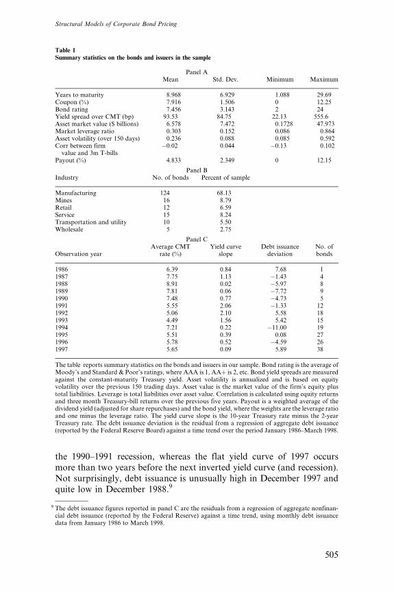
the 1990–1991 recession, whereas the flat yield curve of 1997 occurs

more than two years before the next inverted yield curve (and recession).

Not surprisingly, debt issuance is unusually high in December 1997 and

quite low in December 1988.9

Table 1Summary statistics on the bonds and issuers in the sample

Panel AMean Std. Dev. Minimum Maximum

Years to maturity 8.968 6.929 1.088 29.69Coupon (%) 7.916 1.506 0 12.25Bond rating 7.456 3.143 2 24Yield spread over CMT (bp) 93.53 84.75 22.13 555.6Asset market value ($ billions) 6.578 7.472 0.1728 47.973Market leverage ratio 0.303 0.152 0.086 0.864Asset volatility (over 150 days) 0.236 0.088 0.085 0.592Corr between firmvalue and 3m T-bills

�0.02 0.044 �0.13 0.102

Payout (%) 4.833 2.349 0 12.15

Panel BIndustry No. of bonds Percent of sample

Manufacturing 124 68.13Mines 16 8.79Retail 12 6.59Service 15 8.24Transportation and utility 10 5.50Wholesale 5 2.75

Panel C

Observation yearAverage CMT

rate (%)Yield curve

slopeDebt issuancedeviation

No. ofbonds

1986 6.39 0.84 7.68 11987 7.75 1.13 �1.43 41988 8.91 0.02 �5.97 81989 7.81 0.06 �7.72 91990 7.48 0.77 �4.73 51991 5.55 2.06 �1.33 121992 5.06 2.10 5.58 181993 4.49 1.56 5.42 151994 7.21 0.22 �11.00 191995 5.51 0.39 0.08 271996 5.78 0.52 �4.59 261997 5.65 0.09 5.89 38

The table reports summary statistics on the bonds and issuers in our sample. Bond rating is the average ofMoody’s and Standard & Poor’s ratings, where AAA is 1, AAþ is 2, etc. Bond yield spreads are measuredagainst the constant-maturity Treasury yield. Asset volatility is annualized and is based on equityvolatility over the previous 150 trading days. Asset value is the market value of the firm’s equity plustotal liabilities. Leverage is total liabilities over asset value. Correlation is calculated using equity returnsand three month Treasury-bill returns over the previous five years. Payout is a weighted average of thedividend yield (adjusted for share repurchases) and the bond yield, where the weights are the leverage ratioand one minus the leverage ratio. The yield curve slope is the 10-year Treasury rate minus the 2-yearTreasury rate. The debt issuance deviation is the residual from a regression of aggregate debt issuance(reported by the Federal Reserve Board) against a time trend over the period January 1986–March 1998.

9 The debt issuance figures reported in panel C are the residuals from a regression of aggregate nonfinan-cial debt issuance (reported by the Federal Reserve) against a time trend, using monthly debt issuancedata from January 1986 to March 1998.


505

Because our sample may be considered unusual in that each firm has a

simple capital structure, one may wonder if these bonds are representa-

tive of the overall bond market. A comparison of our bonds with the

7531 noncallable and nonputable bonds from nonfinancial, nonregu-

lated industries suggests that they are. The two samples have very similartime-series patterns and similar fractions of below-investment-grade

bonds (more than 90% of all noncallable bonds are investment grade).

Our sample has a slight tendency toward safer companies, and thus

toward yields that are a tad lower (7.4% compared to 7.6% for the

larger sample). The average bond maturity in our sample is two years

shorter than the average overall, reflecting the fact that our longest bond

has a maturity that is just under 30 years, and our sample has no century

bonds.Data on bond features are taken from the Fixed Income Database; data

on balance sheets and other accounting data are from Compustat; share

prices, dividend yields, and the number of shares outstanding are from

CRSP. Interest rate data are from the CMT series reported in the Federal

Reserve Board’s H15 release.

2. Implementations

In this section we first discuss very briefly the implementation of the

five models. We then describe how we estimate parameters for thesemodels.

Each of the models has an analytical or quasi-analytical formula for

coupon bond prices. Except for the G model, all the pricing formulas

are straightforward to implement and are given in Appendix A for the

reader’s convenience. The Geske formula involves multivariate normal

integrals and is not straightforward to implement accurately, especially

for long-maturity bonds. Following Huang (1997), we choose to obtain

the bond prices for the G model using the binomial method (finitedifference methods can also be used). Once we have a set of

bond prices predicted by the models, we calculate the corresponding

predicted yields as bond equivalent yields assuming semiannual

compounding.

Each of the structural models has a set of parameters that must be

estimated. Parameters related to firm value and capital structure include

the initial levels of debt and assets, the payout parameter, asset return

volatility, the speed of a mean-reverting leverage process, and those para-meters that characterize the target leverage ratio. In addition, implemen-

tation of the models requires estimates of parameters that define the

default-free term structure, as well as parameters related to bond char-

acteristics. Below we discuss how to estimate the three types of parameters

that are summarized in Table 2.


506

2.1 Firm value and capital structure parameters

Rather than using the face value of the bond to calculate the default

boundary in these models, we use the book value of total liabilities

reported in the firm’s balance sheet. In most structural models, equity

holders earn the residual value of the firm once debt is paid off. Oftenthe payoff amount is assumed to be the face value of the bond being

priced. However, equity residual values only begin to accrue once the

par value of the bond is paid if there is no other debt in the firm, and

the firms in our sample have other debt. Thus all the debt must be

paid off before equity has any value. To calculate a leverage ratio, we

also need the asset value. This can be estimated as the sum of the

Table 2Estimation of model parameters

Parameter Description Estimated as Data source

Bond featuresc Coupon Given FIDT Maturity Given FIDF Face value Total liabilities Compustatw Recovery rate Given Moody’s

Firm characteristicsV Firm value Total liabilities plus

market value of equityCompustat and CRSP

mv Asset returns Average monthlychange in V

Compustat and CRSP

sv Asset volatility Historical equity volatilityadjusted for leverage

Compustat and CRSP

d Payout ratio Weighted average of cand the sharerepurchase-adjusteddividend yield

Compustat, CRSPand FID

k‘ Speed of adjustmentto target leverage

Coefficient from aregression of changesin log leverage againstlagged leverage and r

CRSP, CMT andCompustat

f Sensitivity of targetleverage tointerest rates

Coefficient from aregression of changesin log leverage againstlagged leverage and r

CRSP, CMT andCompustat

t Tax rate Assumed at 0.35 —

Interest ratesr Risk-free rate NS or Vasicek models CMTr Correlation between

V and rCorrelation betweenequity returnsand r

CRSP and CMT

sr Interest rate volatility Vasicek model CMT

FID is the Fixed Income Database. CRSP is the Center for Research in Security Prices database. CMT isthe constant maturity Treasury rate series available on the Federal Reserve Board’s website. NS refers tothe Nelson and Siegel (1987) model. Total liabilities are used for the default boundaries in most instances,but sensitivity to the assumption is also shown by using the KMV measure of liabilities. Likewise, we alsoshow the sensitivity of the estimates to using historical equity volatility by estimating the models withimplied volatility and future volatility.


507

market value of equity and the market value of total debt, the latter

being proxied by its book value.10 The leverage is then measured as

total liabilities over the sum of total liabilities and market value of

equity. To show the sensitivity of structural models to the leverage

ratio, we also implement the LS model using a measure of leveragesuggested by KMV Corporation [see Crosbie and Bohn (2002)]11 and

we examine implied leverage ratios from the LS model as well.

Parameters k‘ (the mean-reverting parameter), f (characterizing the

sensitivity of the leverage ratio to interest rates), and n (related to the

target leverage) can be estimated by regressing leverage on lagged leverage

and interest rates. See Appendix B.2 for more details.

Parameter d measures a firm’s yearly payout ratio. This parameter is

not part of the original M, G, or LSmodels, but can easily be added. In theCDG model, the effect of the payout ratio is exactly canceled by the

inclusion of a target debt ratio, and the results are the same whether we

use the firm’s past payout level or assume no payout (see below for more

details). The variable d is meant to capture the payouts that the firm

makes in the form of dividends, share repurchase, and bond coupons to

equity holders and bondholders. To obtain a good approximation of the

value of d, one must know the firm’s leverage, its dividend yield, its share

repurchases, and the coupon on its debt. We calculate d as a weightedaverage of the bond’s coupon and the firm’s equity payout ratio, where the

weights are leverage and one minus leverage. The equity payout ratio is

the dividend yield for firms with no share repurchases in the year of the

bond observation, but otherwise the dividend yield is grossed up by the

ratio of share repurchases to dividends. If there are no dividends and only

share repurchases, a share repurchase yield is calculated for the equity

portion of the payout ratio. Share repurchases and yearly dividend levels

are reported on Compustat.A key input parameter in a structural model is sv, the asset return

volatility, which is unobservable. Asset volatility can be measured by

using historical equity volatility and leverage or we can measure asset

volatility from bond prices observed at a different point in time. The

latter, bond-implied volatility, is analogous to the Black and Scholes

implied equity volatility used in option markets. Detailed discussions of

these volatility measures are provided in Appendix B.1. We implemented

the five structural models using seven estimates of volatility: bond-impliedvolatility from the previous month’s bond price, which is always in

November in this sample, and six estimates of volatility based on

equity returns. The latter include measures of volatility using 30, 60, 90,

10 Given that most of the bond prices are close to par, this approximation is expected to be reasonable.

11 KMV is a subsidiary of Moody’s.


508

and 150 trading days before the bond price observation and one based on

equity prices over 150 trading days after the bond price is observed, on the

assumption that some of the future path of equity price volatility can

be anticipated. The sixth equity-based estimate uses the GARCH(1,1)

[Bollerslev (1986)] model and 150 days of prior equity returns. Exceptfor those based on bond-implied volatility, the differences in average

errors among the various measures are small and largely reflect outliers

that occur more often with the shorter windows. We discuss the results of

bond implied volatility in more detail in the appendix, but for the sake of

brevity in the remainder of the article we report only results for historical

volatility based on 150 trading days.

2.2 Interest rate parameters

Interest rate parameters on a given day are estimated using the CMT

yield data on that day or over the previous month. (The CMT series,

published by the Federal Reserve, is largely a historical series of on-the-

run Treasury yields, and is described in more detail on the Federal

Reserve Board’s web page.) We estimate interest rate parameters either

by fitting the Nelson and Siegel (1987; hereafter NS) yield curve model

or the Vasicek (1977) model to the CMT yields (see Appendix B.3 formore details).12

In the one-factor models of G and LT, the risk-free rate is estimated

using the rate from the NS model for a Treasury bond with the same

maturity as the corporate bond being priced. For the M model, each

coupon is priced with the spot rate whose maturity matches the date of

the coupon. In the base case, the NS model is used to generate spot

rates. For the sake of comparison, the Vasicek model is also used to

calculate spot rates in the M model. In both LS and CDG, interestrate dynamics are described by the Vasicek model; thus we implement

these two models using Vasicek estimates to ensure their internal

consistency.

The correlation coefficient r between asset returns and interest rates in

both LS and CDG is approximated by the correlation between equity

returns and changes in interest rates. We use 3-month Treasury-bill rates

and stock price data over a window of five years in the correlation

estimations.

12 It should be noted that the use of a yield curve model introduces errors in the risk-free rate used as thebenchmark for calculating the spread. We ignore the term structure errors when calculating spreadprediction errors, as both the predicted yield and the predicted risk-free rate have the same error and itis eliminated with subtraction. While there is no easy way to correct for this additional source of error, itdoes raise the question of which risk-free rate should be used by a practitioner who prefers to haveestimates of yields.


509

2.3 Parameters related to bond features

Another key input parameter in a structural model is the recovery rate w.

Research on recovery rates by Keenan, Shtogrin, and Sobehart (1999)

indicates that the average bond recovery rate is 51.31% of face value

[see also Altman and Kishore (1996)]. While this figure is conceptuallystraightforward, its components are not: Some of the loss comes from a

decline in firm value and some from the deadweight costs of financial

distress. In models with endogenous recovery rates, the two components

can be specified separately. Leland and Toft assume that liquidation

values are about half of firm value (implying a deadweight cost of 50%),

but this figure is still a source of debate in the corporate finance literature

[see Andrade and Kaplan (1998)]. Alderson and Betker (1996) analyze

estimates provided in bankruptcy cases and conclude that liquidationvalues are no less than 63% of going concern values. Andrade and Kaplan

(1998), however, suggest that the costs of financial distress are lower,

likely in the range of 15–20%.

In the original M and G models, bondholders receive 100% of the

firm’s value in the event of default. In contrast, LT explicitly assumes

that bondholders receive only a fraction of the assets in default. In the

LS and CDG models, recovery rates as a fraction of face value are, by

definition, identical to recovery rates as a fraction of asset value. Tofollow market convention and to make the results comparable across

models, we implement the 51.31% of face value specification for all of

the models. However, we also implement the G model with recovery

equal to 100% of firm value to show the effects of the face value

assumption.

Among the five models examined in the article, the LT model is the only

one that considers taxes by incorporating the tax deductibility of interest

payments in the model. Following them, we choose a value of the tax ratet ¼ 0.35.

3. Empirical Results

In Section 3.1 we discuss the ability of the models to fit market prices. We

present the percentage pricing errors, the percentage errors in yields, and

the percentage errors in yield spreads. We consider the error in spreads

to be the most informative measure of model performance because the

corporate bond yield is expected to be greater than the Treasury yield in

every model.13 In addition, we pay particular attention to the standard

13 Suppose a corporate bond trades at a yield to maturity (YTM) of 6.5% and a comparable maturityTreasury has a YTM of 6%. A good test of the model is whether it can explain the 50 basis point spread.If the model predicts a YTM of 6.1%, then the spread prediction error is �80%, but the the error as afraction of yield seems small (about �6%). Any model would predict a YTM above 6%, so the percentageerror in yields is crediting the model with more predictive power than reasonable. The situation is similarfor the pricing errors.


510

deviation of the spread prediction errors and the average absolute spread

prediction errors because all of the models have substantial dispersion in

predicted spreads. In Section 3.2 we examine if these models have sys-

tematic prediction errors.

3.1 Predicted spreads from the structural models

Table 3 summarizes the prediction errors of the five models. For each of

the measures of pricing errors in columns 2 through 7, the numbers in

parentheses are standard deviations of the prediction errors. Columns 2,

4, and 6 show measures of model errors, whereas columns 3, 5, and 7 showthe absolute values of the errors. We focus our analysis on columns 6 and

7, which report errors in credit spreads.

3.1.1 One-factor models. The first row of this table shows that the M

model overprices bonds on average. Our results suggest somewhat less

overpricing of bonds than those found by JMR, a difference probably

due to our use of a payout ratio and a cost of financial distress (by

assuming the recovery rate is 51.31% of face value). When measuredby the yield spread error, the average error is negative and indicates

that the model has only modest predictive power. All of the spread

prediction errors in this table are significantly different from zero.

The estimates for the M model reported in Table 3 are based on

risk-free rates from the NS model. Given that some models must use

Vasicek estimates, one wonders whether the NS model provides sig-

nificant benefits. We implemented the M model using rates from the

Vasicek model (not shown) and found that the average spread predic-tion error scarcely differs from that shown in Table 3.

Panels A–C of Figure 1 plot the predicted bond spreads from the M

model and the actual bond spreads against maturity for three rating

classes. Panel A shows the predictions of the model for bonds rated A

or higher; panel B shows BBB-rated bonds; and panel C plots the

market and predicted spreads of bonds that are rated below investment

grade. All of the rating classes have many examples of extreme over-

prediction and extreme underprediction of bond spreads, although thecases of underprediction are far more numerous. The tendency toward

underprediction appears to be somewhat stronger among the short-

maturity bonds, but this pattern only appears in bonds rated BBB or

higher.

The ‘‘portfolio of zeroes’’ approach that we use in the Mmodel (and the

LS and CDG models) is simple to implement but treats these ‘‘zeroes’’

(coupons) as independent of each other. The G model provides a more

rigorous treatment of coupons. Rows 2 and 3 of Table 3 show the predic-tions from the G model. The results in row 2 assume bondholders receive


511

Table

3Perform

ance

ofthestructuralmodels

Bondpricing

model

Percentage

pricingerror,

mean

(std.dev.)

Absolute

percentage

pricingerror,

mean

(std.dev.)

Percentageerror

inyield,

mean

(std.dev.)

Absolute

percentage

errorin

yield,

mean

(std.dev.)

Percentageerror

inspread,

mean

(std.dev.)

Absolute

percentage

errorin

spread,

mean

(std.dev.)

Merton

1.69%

(4.94%)

3.67%

(3.71%)

�91.30%

(17.05%)

91.84%

(13.84%)

�50.42%

(71.84%)

78.02%

(39.96%)

Geske(face

recovery)

0.70%

(4.89%)

3.22%

(3.73%)

�1.71%

(15.28%)

8.45%

(12.83%)

�29.57%

(74.06%)

66.93%

(43.12%)

Geske(firm

recovery)

2.09%

(3.97%)

3.11%

(3.23%)

�5.47%

(8.46%)

7.58%

(6.62%)

�52.92%

(48.28%)

65.73%

(28.34%)

Leland-Toft

�1.97%

(7.54%)

4.06%

(6.64%)

15.60%

(74.74%)

19.06%

(73.92%)

115.69%

(490.19%)

146.05%

(481.97%)

LS(1-dayCMT)

�2.69%

(8.19%)

5.63%

(6.51%)

6.62%

(24.85%)

15.02%

(20.86%)

42.93%

(171.63%)

124.83%

(125.07%)

LS(1-m

onth

CMT)

�0.68%

(6.94%)

4.56%

(5.26%)

1.52%

(21.17%)

11.90%

(17.55%)

�6.63%

(132.53%)

96.83%

(90.44%)

CDG

(baseline)

�11.21%

(13.12%)

12.64%

(11.75%)

32.06%

(44.41%)

36.74%

(40.60%)

269.78%

(370.41%)

319.31%

(328.42%)

CDG

(low

k)

�10.50%

(13.03%)

12.09%

(11.56%)

30.09%

(43.82%)

35.14%

(39.86%)

251.12%

(362.73%)

304.32%

(319.16%)

CDG

(low

m)

�3.76%

(10.13%)

7.35%

(7.90%)

11.00%

(31.39%)

20.17%

(26.42%)

78.99%

(247.95%)

170.16%

(196.57%)

Thetablereportsmeansandstandard

deviationsofthepercentageerrors

inthemodels’predictions.Thepercentageerrors

inprices,yields,andspreads,aswellastheirabsolute

values,are

calculatedasthepredictedspread(yield,price)minustheobserved

spread(yield,price)divided

bytheobserved

spread(yield,price).Theerrorsare

those

generatedfrom

implementingthemodelsusing182bondswithsimplecapitalstructuresduring1986–1997withtheassumptionthatrecoveryratesare

51.31%

offace

valuein

defaultandthatasset

volatility

ismeasuredusing150-dayhistoricalvolatility.


512

51.31% of the face value of debt, which is an assumption we will use

throughout the article. In the next row, we assume that there are no

costs of financial distress, so that bondholders receive the entire value of

the firm in default.14

0 5 10 15 20 25 30

250

99

24

0

A: Predicted vs. Actual for Bonds Rated A or Higher

maturity

basi

s po

ints

0 5 10 15 20 25 30

320

99

24

0

B: Predicted vs. Actual for BBB-rated Bonds

maturity

basi

s po

ints

0 5 10 15 20 25 300

200

400

800

1200

C: Predicted vs. Actual for Junk Bonds

maturity

basi

s po

ints

actual spreadpredicted spread

Figure 1Predicted and actual spreads versus years to maturity: theMertonmodel. The actual and predicted spreadsfor the sample of 182 bonds with simple capital structures at year-end during the period 1986–1997. Thespreads are plotted against the remaining years tomaturity of the bond. The actual spreads aremarkedwithan asterisk and the predicted spreads from the Merton model are denoted with a square. Spreads arecalculated in basis points over the Nelson and Siegel (1987) estimates of the Treasury yield curve.

14 In this model as well as the M and LT models, we actually use the recovery rule min(51.31% of par, firmvalue), so that the recovery cannot be higher than firm value. Other estimates, not shown, indicate thatthe firms receiving less than 51.31% of face value are a small fraction of the sample and the averagerecovery is still close to 51.31%. In addition, we impose the constraint that recovery cannot be more thanthe amount owed to bondholders.


513

The average spread prediction error in row 2 of Table 3 is markedly less

negative than the average error in the M model under the same recovery

assumption. This suggests that the compound option approach to cou-

pons in the G model is an improvement over the ‘‘portfolio of zeroes’’

simplification. This may be due to the equity-holders’ option to pay thecoupon, which is incorporated into the G model but ignored in the M

model. If shareholders believe it is worthwhile to pay the coupon when the

firm is actually insolvent (believing it has a good chance to bounce back),

then bondholders face a greater risk of loss (they recover less than they

would at the onset of distress). This effect is more important as maturity

lengthens, all else being constant (there is more time for the firm to

continue a downward spiral). As few junk companies have long-maturity

bonds, the effect of the coupon treatment will be smaller for the bondswith high predicted spreads, and this helps the accuracy of the G model

(see panels A and B of Figures 1 and 2).

This optionality also automatically takes into account conditional

probabilities of default, which are not incorporated in the simple portfolio

of zeroes approach. In the latter method, the calculation of the value of

each coupon ignores whether previous coupons have been paid or not.

This overestimates the probability of default for the firm. Consequently

the variance of the estimated spreads may widen because the firms withthe highest probability of default are affected by this error the most.

The G model’s option to continue relies on financing with new equity

issuance, whereas Ho and Singer (1982) allow coupons to be paid from

asset sales. Such financing is even more damaging to bondholders if

distress occurs. The impact is expected to be greater for high-grade

bonds because they have weaker covenants [Kahan and Tuckman

(1993)]. Of the 31 bonds in our sample for which information is available

on the SEC’s website, only 2 have covenants preventing this behavior, andonly these were rated speculative grade at issuance. While the effect may

be small, the variation among the covenants would help reduce the dis-

persion in spread prediction errors.

In our implementations of the five models, we always assume that

bondholders receive a face value recovery rate of 51.31%. We do so

because two of the models (LS and CDG) do not allow an alternative

rule, making it possible that the other models outperform LS and CDG

only because of the added flexibility in specifying recoveries. To showmore clearly how recovery rates matter, we implement the G model with

and without costs of financial distress. In row 2 we assume bondholders

receive 51.31% of face value (which implies a cost of financial distress of

about 33%) while in row 3, we assume bondholders receive 100% of the

value of the firm (zero cost of distress). Including costs of financial distress

in row 2 results in substantially higher average spreads, but with a loss of

accuracy (which is apparent from the higher absolute spread errors, as


514

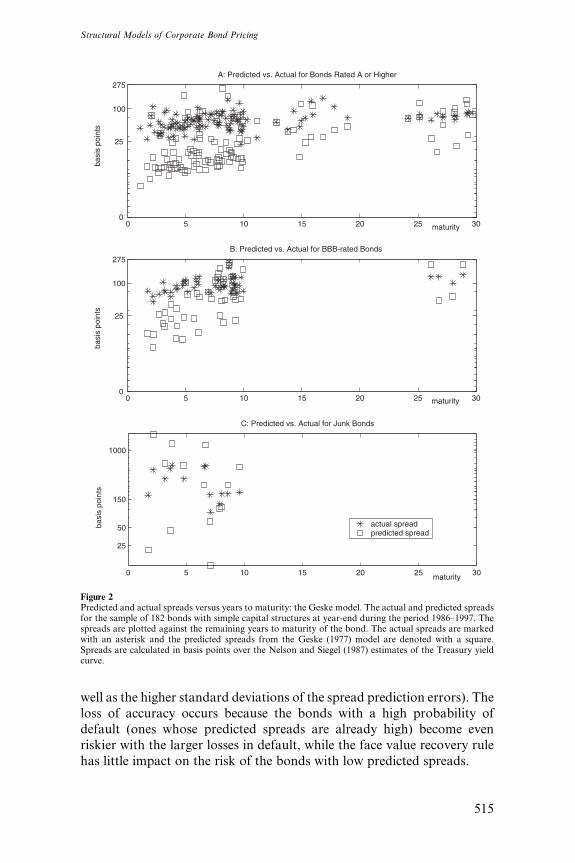
well as the higher standard deviations of the spread prediction errors). The

loss of accuracy occurs because the bonds with a high probability ofdefault (ones whose predicted spreads are already high) become even

riskier with the larger losses in default, while the face value recovery rule

has little impact on the risk of the bonds with low predicted spreads.

0 5 10 15 20 25 30

275

100

25

0


maturity

basi

s po

ints

0 5 10 15 20 25 30

275

100

25

0


maturity

basi

s po

ints

0 5 10 15 20 25 30

25

50

150

1000


maturity

basi

s po

ints


Figure 2Predicted and actual spreads versus years to maturity: the Geske model. The actual and predicted spreadsfor the sample of 182 bonds with simple capital structures at year-end during the period 1986–1997. Thespreads are plotted against the remaining years to maturity of the bond. The actual spreads are markedwith an asterisk and the predicted spreads from the Geske (1977) model are denoted with a square.Spreads are calculated in basis points over the Nelson and Siegel (1987) estimates of the Treasury yieldcurve.


515

To further illustrate this effect on the dispersion of the predicted

spreads, consider the predictions in rows 2 and 3 of Table 3. The average

spread predicted by the G model without distress costs is only 53 basis

points, or slightly more than half the actual average spread of 93 basis

points, whereas the average spread predicted by the model with distresscosts is 85 basis points (the medians suggest a similar effect). The actual

market spreads range from 22 basis points to a high of 556 basis points.

Both implementations result in predictions for dozens of bonds that are

less than 10 basis points, although there are somewhat fewer such cases

when distress costs are included. The more extreme differences in predic-

tions occur among the riskier bonds. The highest predicted spread for the

model with full recovery is 1184 basis points and the second highest

predicted spread is 647 basis points (belonging to the bond with the high-est actual spread). While these estimates are too high, they are much closer

than the estimates from assuming costs of financial distress, which reach

1838 basis points (see Figure 2). Assuming costs of financial distress does

help avoid the problem of underprediction of spreads to a large extent, but

unfortunately increases the variance of the predicted spreads by extreme

overprediction of spreads on the bonds that the model considers to be very

risky. A better approach might be to allow costs of financial distress that

vary among the bond issuers.Figure 2 shows the predicted bond spreads from the Gmodel (assuming

51.31% face value recovery). Like the M model, there is evidence of both

extreme underprediction of spreads and extreme overprediction, but the

problem is less severe here. The G model does better on short-maturity

bonds than the M model does. It also has a greater tendency toward

overprediction of short-maturity junk bonds, although this group is extre-

mely small.

The results from the Gmodel suggest the compound option approach isa major improvement over the portfolio of zeroes treatment used in theM,

LS, and CDG models. The LT model also views coupon bonds as com-

pound options, but has the additional advantage that it has an easy-to-

implement closed-form solution.

The LT model, shown in row 4 of Table 3, has a serious tendency to

overpredict bond spreads. Every volatility measure that we used in the

implementation of the LT model (only one is shown) resulted in a sig-

nificantly positive average spread prediction error. Moreover, the medianof the spread prediction errors summarized in Table 3 is 36% and nearly

two-thirds of those spreads are overestimated. However, the standard

deviation and the absolute prediction errors indicate a dramatic lack of

accuracy.

The LT model predicts a spread for the average bond in our sample that

is more than twice the spread actually observed in the market. The highest

predicted spread is 5096 basis points, which although way off the mark, at


516

least belongs to a bond with a market spread of 465 basis points (see

Figure 3). Less comforting is the fact that the second highest predicted

spread, 4655 basis points, belongs to a bond that only trades at a spread of

75 basis points.

0 5 10 15 20 25 30

10000

2500

275

99

24

0


maturity

basi

s po

ints

0 5 10 15 20 25 30

400

99

24

0


maturity

basi

s po

ints

0 5 10 15 20 25 30

10000

2500

275

99

24

0


maturity

basi

s po

ints

predicted spreadactual spread

Figure 3Predicted and actual spreads versus years to maturity: the LT model. The actual and predicted spreads forthe sample of 182 bonds with simple capital structures at year-end during the period 1986–1997. Thespreads are plotted against the remaining years to maturity of the bond. The actual spreads are markedwith an asterisk and the predicted spreads from the Leland and Toft (1996) model are denoted with asquare. Spreads are calculated in basis points over the Nelson and Siegel (1987) estimates of the Treasuryyield curve.


517

The LT model’s assumption of a continuous coupon sharply

increases the probability of default on high-coupon bonds. Consider

the sole zero-coupon bond in our sample (we set its coupon to one basis

point to implement the model). This bond is one of the riskiest in the

sample: its market spread is 488 basis points, it is rated B3/CCCþ, andboth its leverage ratio and asset volatility are above average. Even the

M model, which has trouble generating double-digit spreads at all,

predicts a spread of 45 basis points for this bond. Yet the LT model

generates a predicted yield spread of essentially zero for this bond

because the coupon is virtually zero. In contrast, a bond rated AA/

Aa2, which has below-average volatility and below-average leverage,

carries a market spread of only 62 basis points, but the LT model

estimates this bond’s spread at 50 basis points. The higher spread oweslargely to its 9.25% coupon, which was set at a time when Treasury

rates were higher.

Figure 3 shows the predicted spreads of the LT model in comparison

to the actual bond spreads. In panel A, the highest predicted spread for

a bond rated A or higher is 4655 basis points, which tends to obscure

the pattern in other high-grade bonds. Excepting this extreme outlier,

the LT model reveals a tendency toward overprediction of spreads that

is highest at short maturities. This bias exists for all three rating groups,but is extreme with junk bonds, almost implying a strict downward-

sloping credit yield curve. For the investment-grade bonds, the model

tends to either overpredict short-maturity bond spreads or to severely

underpredict them, while the longer-maturity bonds are priced more

accurately.

We have considered the predictive power of three one-factor models,

each of which was created without regard for the stochastic nature of risk-

free interest rates. Two of these tend to predict spreads that are too lowrelative to the market, while the third usually overestimates credit risk. Of

the three models, only the M model is implemented with any sense of

variation in the risk-free rate, yet it is only the LT model with a constant

Treasury rate that generates high spreads on average. In the balance of

Section 3.1 we consider the impact of explicitly incorporating stochastic

interest rates into the structural models.

3.1.2 Two-factor models. The last five rows of Table 3 summarize the

results from implementing the LS and CDG two-factor models. Rows 5

and 6 report results for the LS model using two different data sources for

the Vasicek model parameters (in row 5, the Vasicek model is estimated

using Treasury yields from one day, while in row 6, the model estimates

are based on data throughout the month of December). In the implemen-tation of the CDGmodel, shown in rows 7–9, we use the Vasicek estimates

based on one day’s data.


518

The CDG model differs from the LS model in the assumption of a

target leverage ratio. We implement the version of the CDG model that

assumes that the target depends on interest rates (the two-factor model).

To show the sensitivity of the CDG model to parameter choices, we

present results from three implementations: row 7 of Table 3 is basedon parameters that are estimated from the sample firms’ data. These

parameters include the firm’s mean asset return and the speed of

adjustment toward the target leverage ratio. Row 8 assumes a lower

speed of adjustment to the mean and row 9 assumes a lower mean asset

return.

Both the LS and CDGmodels have much higher predicted spreads than

either the M or G models, and in most implementations (varying in the

choice of equity volatility) the average spread error is positive (the averagespread error for the LS model shown in row 6 is the lone negative figure).

The estimates for the CDG model reveal a strong tendency toward over-

estimation of spreads, which is only somewhat mitigated in the last two

rows of the table.

The higher average spreads in these two-factor models appear to be a

major improvement over the M and G models. However, they come at a

substantial expense to accuracy. The absolute spread errors of the LS

model in row 5 of Table 3 are nearly double those of the M and G modelsunder the same recovery rate assumption, and they are even higher in the

CDG model. The LS and CDG models have substantially fewer bonds

that suffer from the kind of serious spread underprediction problem seen

in theMmodel. The median spread error in the LS model using one day to

estimate Vasicek is�13%, compared to�62% and�72% for the G andM

models, respectively. The median predicted yield spread for the CDG

model under the same assumptions is even higher (218 basis points versus

77 basis points for the LS model).While these two-factor models have truly higher predicted spreads, the

range of predicted spreads is extreme: there are 34 bonds for which the

LS model’s prediction is less than 1 basis point, including 11 bonds where

the predicted spread is so close to zero that the prediction error is

reported as �100%. The CDG model shown in row 7 can boost the

spreads of some of these bonds, as only 22 bonds have a predicted spread

of less than 1 basis points and only 10 bonds have a reported error of

�100%. In contrast, the lowest predicted spread in the G model is 3 basispoints. At the other end of the credit spectrum, the results are equally

extreme. The highest predicted spread for CDG is 3179 basis points,

quite a bit more than the 2161 basis points predicted for that bond by

the LS model, which itself is still much higher than any spread actually

found in the sample (see Figures 4 and 5).

We can identify a number of factors that are likely to cause

this tremendous dispersion in predicted spreads: the assumption of an


519

exogenous default boundary, face value recovery rates, the failure to

adjust this portfolio of zeroes approach for conditional probabilities of

default, and the use of the Vasicek model. The flat default boundary in LS

is likely to make a risky bond even more risky, with little impact on the

0 5 10 15 20 25 30

625

99

24

0


maturity

basi

s po

ints

0 5 10 15 20 25 30

1100

275

99

24

0


maturity

basi

s po

ints

0 5 10 15 20 25 30

10

100

500

1000

2000C: Predicted vs. Actual for Junk Bonds

maturity

basi

s po

ints


Figure 4Predicted and actual spreads versus years to maturity: the LS model. The actual and predicted spreads forthe sample of 182 bonds with simple capital structures at year-end during the period 1986–1997. Thespreads are plotted against the remaining years to maturity of the bond. The actual spreads are markedwith an asterisk and the predicted spreads from the Longstaff and Schwartz (1995) model are denotedwith a square. Spreads are calculated in basis points over the Vasicek (1977) estimates of the Treasuryyield curve.


520

credit risk of a safe bond. We saw in our analysis of the Gmodel, where we

were able to hold all other features of the model constant, that the face

value recovery rate adds markedly to the dispersion of predicted spreads.Neither the LS and CDG models nor the coupon version of the M model

that we implement can reasonably incorporate a recovery rate based on

0 5 10 15 20 25 30

1111

275

99

24

0


maturity

basi

s po

ints

0 5 10 15 20 25 30

2500

275

99

24

0


maturity

basi

s po

ints

0 5 10 15 20 25 30

24

99

275

3000 C: Predicted vs. Actual for Junk Bonds

maturity

basi

s po

ints


Figure 5Predicted and actual spreads versus years to maturity: the CDG model. The actual and predicted spreadsfor the sample of 182 bonds with simple capital structures at year-end during the period 1986–1997. Thespreads are plotted against the remaining years to maturity of the bond. The actual spreads are markedwith an asterisk and the predicted spreads from the Collin-Dufresne and Goldstein (2001) model aredenoted with a square. Spreads are calculated in basis points over the Vasicek (1977) estimates of theTreasury yield curve.


521

firm value.15 A related issue for these two models is how to implement the

face value recovery rate rule. Under the simple portfolio of zeroes

approach, a default results in bondholders recovering a fraction of the

coupon on every future coupon date. This is not consistent with bank-

ruptcy practices. Lastly, as we noted earlier, this portfolio of zeroesapproach overestimates the probability of default in assuming indepen-

dence of the coupons. This may lead to dispersion because the bonds that

are already considered risky by the model (i.e., those with a high prob-

ability of default on their early coupons) will have an even greater prob-

ability of default associated with them, while there are no bonds that

would be considered safer as a result.

The LS and CDGmodels may lose accuracy from the use of the Vasicek

model if the interest rate volatility is poorly estimated in this model.16 Inrow 6 of Table 3, we show the sensitivity of the LS model to the estimates

of the Vasicek model. The implementation in this row uses Treasury data

from the entire month in which the bond trades, rather than just a single

day. The estimates based on one month of data lead to much lower

estimates of interest rate volatility.

The two sets of estimates for the LS model in Table 3 differ both in

average predicted spreads and the degree of dispersion in predicted

spreads. Consider the estimates for 1997, when the estimate of volatilityis 34% using one-day data and is nearly zero using the time-series data.

The former group includes six bonds that have predicted spreads of less

than a basis point, whereas the less volatile interest rate dynamics result in

nine such bonds. Nearly all of the spread estimates for the 1997 sample

increase when estimated interest rate volatility rises, but the higher

volatility actually exacerbates the overprediction problems on the riskiest

bonds with only a small impact on the safest bonds.

The predicted spreads from the LS model from row 5 of Table 3 areshown in Figure 4, plotted against maturity for the three rating groups.

Relative to the actual spreads, the LS has a tendency to predict either a

very high spread or a very low spread. More often the highest predicted

spreads belong to the lowest rated bonds. The dispersion is also more

extreme at the shorter maturities, especially in the range of 5–10 years.

The CDG model also exhibits wide dispersion in predicted spreads, but

this model differs markedly from the LS model in its predictions for the

portion of the sample that have market spreads between 75 and 200 basispoints (there are 79 bonds in this group). The CDG model clearly raises

15 In results not reported, we implemented the LS model with recovery rates that vary by industry [usingdata from Altman and Kishore (1996)], but like Lyden and Saraniti (2000), we find it does not improvethe estimates.

16 Chan et al. (1992) conclude that the Vasicek model is a poor fit for the short-term rate and note that thefit is particularly sensitive to the level of interest rates.


522

the spread on the typical bond relative to the LS model. The latter model

predicts spreads of less than 10 basis points for 10 of these bonds (only 3 in

the CDG model) and underpredicts the spread for 35 bonds (only 16

bonds in the CDG model). Of these 79 bonds, the CDG model predicts

a spread that is more than double the actual spread for 54 of the bonds,compared to only 27 for the LS model.

Indeed, the results in Table 3 suggest that the CDG model severely

overestimates credit risk. Possibly the model might be better implemented

with other estimates for the parameters related to the target leverage ratio,

such as the speed of adjustment (k‘) and mean asset returns.

We estimate an average speed of adjustment factor of .10, which is

markedly less than the .145 found by Frank and Goyal (2003). Our

average may differ because our sample includes more firms from the1990s. However, raising k‘ would lead to even higher spread errors. In

row 8 we show the impact on predicted spreads of lowering each estimated

k‘ by 15% (the average k‘ falls from .10 to .085). The estimates shown in

row 8 indicate that, for the level of k‘ observed in our sample, the effects of

mismeasurement of the speed of adjustment are small. The average spread

prediction error falls only by 15–20 percentage points, from a base of 270

percentage points. Lowering k‘ further would make it closer to zero,

effectively making the model equivalent to the LS model.The average asset return in our sample is 1.5% per month, only slightly

higher than the median return. Together with our sample’s average divi-

dend yield (adjusted for share repurchases), this implies an annual average

asset return of 24%, which seems high by historical standards. Our sample

starts in 1986 and is dominated by bonds that are priced after 1990, which

likely explains the high estimated returns. However, bond market partici-

pants may not view the high average asset returns of the 1990s as long-

run average rates of return. If so, then a lower mean asset return is moreappropriate in the implementation. In the last row of Table 3 we show

results from reducing each firm’s estimated mean asset return by 45%.

This adjustment makes the average asset return in the sample about equal

to the return that would lead to equity returns observed over longer

periods of time (i.e., consistent with an average equity return of 15% and

an equity risk premium of 6%).

By reducing the mean asset return estimate, the problem of bond price

underestimation is much smaller. Spreads are now overpredicted by only79%. The median yield spread is predicted at only 57 basis points and the

median spread prediction error is �36%. However, the absolute errors

are still quite large, as are the standard deviations. The wide variation in

estimated spreads in the CDG model may reflect the added opportunity

for parameter estimation error. An alternative to using estimates of mean

asset returns and speed of adjustment would be to simply estimate the

implied risk-neutral long-term mean of leverage, which not only fits the


523

data to the spreads, but avoids estimation of the mean asset return in the

model (cf. Appendix B.2).

Figure 5 presents the predicted and actual bond spreads for the CDG

model from row 7 of Table 3. The highest-rated bonds, shown in panel A

of the figure, have a higher fraction of bonds that are considered extremelysafe by the model. However, they are not the majority of the bonds in this

rating class, and the rest of the bonds are credited with too much risk,

especially at the shorter maturities. Bonds rated A or higher also appear to

have overpredicted spreads more often among bonds that mature in 10 or

fewer years, but once maturity extends beyond 10 years, there is no

particular relationship between maturity and spread prediction errors.

3.1.3 Alternative measures of leverage. We have presented pricing

errors from the five structural models using parameters that we consider

reasonable. One could argue that all of the parameters are subject to

measurement error and that the pricing errors are due to the implemen-

tation, and such a complaint would naturally focus on asset volatility

and leverage. While we have ruled out measurement error in assetvolatility as a major issue, we have not yet considered the possibility

that our measure of leverage is causing errors. We next summarize the

sensitivity of the implementations to the choice of the leverage para-

meter. For the sake of brevity, we do not consider this parameter for

every model.

In estimations (not reported), we also used the bond par value as the

strike price in the M model and LS models. Both models had sharply

lower estimated spreads as a result, which is unsurprising once one con-siders the capital structures of the firms in the sample.17

Another possible way to parameterize leverage is suggested by KMV

[see Crosbie and Bohn (2002)], who place a greater weight on short-term

obligations probably for the purpose of better predicting the firm’s default

probability within one year. The logic of this approach is that debts due

in the near term are more likely to cause a default. KMV measure the

numerator of the leverage ratio as short-term debt plus half the value of

long-term debt. Clearly this will also lead to much lower estimates ofcredit spreads unless the sum of short-term debt and long-term debt is

close to total liabilities (as noted earlier, this is not the case in our sample).

The most extreme effect of using KMV’s leverage measure in our sample is

the funeral home firm Hillenbrand, whose liabilities largely consist of

prepaid funeral packages that are sold in the form of insurance. As the

policies are neither long-term nor short-term debt, the inability to honor

17 The median ratio of long-term debt to total liabilities is about 30%, and the median face value of the bondis only $150 million, which is typically a bit more than half of the firm’s long-term debt. Thus, par valuecan easily understate the firm’s obligations by 85%.


524

them would not be considered a source of credit risk by KMV, yet no

bondholder would ignore these obligations.

We implemented the LS model using KMV’s leverage ratio, and as

expected, the lower average leverage leads to much lower predicted

spreads. Despite reducing the average predicted spread, the KMV mea-sure could be very useful. By adding a constant to the spreads generated

by the KMV measure, predicted bond spreads would fit the data better.

For example, the highest predicted spread (without the added constant)

falls from 2161 basis points to 870 basis points in the LS model with the

KMV measure of debt. The lower variance arises because the reduction

in leverage is greatest for the riskiest firms (for bonds rated A or higher,

switching to this method reduces leverage by 7%, compared to a 23%

decrease for junk-rated firms). Partly this reflects the fact that lower-ratedfirms do not participate in the commercial paper market and have less

short-term debt [see Crabbe and Post (1994)].

Another way to consider the sensitivity of the results to the choice of

leverage parameter is to fit the leverage ratio to the bond prices and

examine the implied leverage ratio. We generated implied leverage ratios

for the LS model, and to speed convergence, we allow two bonds from the

same firm on the same day to have different implied leverage ratios. The

average implied leverage ratio obtained for the LS model is 35%, a bithigher than the ratio of total liabilities to assets we have been using. Yet

the average implied leverage ratio is no more informative than the average

spread prediction error. As before, there is substantial variation across

credit ratings. Bonds rated A or higher have an implied leverage ratio that

is 12% higher than the observed leverage ratio, while BBB bonds and junk

bonds have implied leverage ratios that are 5% and 18% below the

observed ratios, respectively (all three figures are statistically different

from zero). Thus, if there is a better leverage parameter that we coulduse, it must be a parameter that raises the leverage of the safe bonds while

simultaneously lowering the leverage of the riskier bonds.

3.2 Systematic prediction errors

In the previous section we mentioned some examples of bonds with

extreme pricing problems. In this section we consider in more detail the

question of why the models’ predictions are inaccurate. We estimate a

multivariate regression analysis of the spread prediction errors to deter-

mine which factors cause the weaknesses in the models. Before theregression stage, however, we narrow the list of potential variables by

conducting t-tests on two subsamples, those with the lowest spread pre-

diction errors and those that have the highest spread prediction errors.

We examine five types of variables that might lead to systematic valua-

tion errors: (1) measures of leverage and capital structure (e.g., bond

ratings, book leverage, long-term debt/total liabilities), (2) variables


525

related to firm value, (3) measures of asset volatility, (4) bond features,

and (5) variables that proxy for differences in expected recovery rates [e.g.,

plant, property and equipment, capital expenditures, and research and

development (R&D)]. We examine 26 variables with t-tests to determine if

any of these areas are problematic in the structural models. Many of thesevariables are already part of the models.

3.2.1 t-Tests to determine systematic errors in spread predictions. Table 4

presents the t-tests for the five structural models. The t-tests examine

differences in characteristics of two groups: those with spread predictionerrors that are below the median in the sample and those that have

prediction errors that are above the median. The errors analyzed in this

table are the percentage differences between the predicted spreads and the

observed spreads.

To present the results in a compact format, we only report signed

t-statistics in Table 4. If the average of a variable is higher in the sample

of bonds with themost positive spread prediction errors, then the t-statistic

will be positive. For example, most models have a significant difference inmaturity between the two subsamples, with the lower spreads associated

with shorter maturity. Then the t-statistic in Table 4 in the maturity row

will be a large positive number.

The results of the t-tests indicate that all of the models have systematic

errors related to leverage, although the problem is less extreme in the

LT model. In general, the models do a poor job of pricing safer bonds.

The bonds with the smallest predicted spreads have a significantly lower

leverage ratio on average (particularly if measured by market leverage).As this factor is included in each of the models, the results suggest that

either leverage is measured poorly or that the models do not assign the

appropriate risk to each level of leverage. Other leverage-related variables

are also significant. For example, the average ratings are sharply different

between the two samples for all but the LT model. The bonds with the

higher predicted spreads are typically rated BBBþ (nine on this scale),

while the bonds with the low predicted spreads have an average rating of

about an A- or an A. Further, the spread underprediction problem istypically less severe for the firms where book value of leverage is close to

the market value of leverage. It appears that firms with very high market

values of equity are often treated by the models as if they are remarkably

safe firms, whereas the bond market is not quite so sanguine about their

prospects.

The t-tests show slight support for CDG’s view, in that the difference

between the current leverage ratio and the 10-year average ratio is close to

statistically significant or actually significant in all but the LT model.When significant, the t-tests are always positive, suggesting that bonds

with high leverage today receive the highest spreads in most of the models,


526

even if the market does not perceive this leverage ratio to be normal over

the longer term.

Table 4 reveals little evidence that systematic errors occur with firm size.

The market values of assets differ significantly in the Mmodel and the LTmodel, but with opposite signs for the two models.

Although the LT model is again an exception, most models have a

strong difference between the market-to-book ratios of the two samples.

As the growth rate of the firm, measured by changes in market value, is

not a source of mispricing, this suggests that market-to-book is not related

to future prospects so much as it is to valuation effects. As many of the

bond prices are observed in the booming equity market of the 1990s,

Table 4t-Tests of prediction errors from defaultable-bond pricing models

Pricing models

ExtendedMerton

Geske Leland-Toft

Longstaff-Schwartz

Collin-Dufresneand Goldstein

Book leverage 2.95 3.03 1.91 2.88 3.06Market leverage 6.47 6.35 2.04 6.23 5.76Abs(market leverage�book leverage) � 4.28 � 4.06 � 0.33 � 4.12 � 3.3910-year mean of leverage 5.28 5.12 1.84 4.90 4.48Current leverage� 10-year mean 1.62 1.69 0.37 1.83 1.81Long-term debt/total liabilities 2.16 1.03 � 1.31 0.73 1.16Bond rating 4.85 4.00 � 0.78 2.41 2.84Difference in ratings 0.22 0.00 � 1.30 0.00 0.22Total assets (book) 0.18 0.82 1.61 1.32 1.09Total assets (market) � 1.73 � 0.82 1.79 � 0.62 � 0.74Asset growth rate 1.43 1.28 � 0.14 0.36 2.70Market/book � 5.90 � 5.29 � 0.30 � 5.47 � 4.52150-day equity volatility 7.99 7.65 � 0.05 5.13 4.90150-day asset volatility 6.70 6.23 � 1.68 4.02 3.69Years to maturity 4.16 2.61 � 0.64 2.46 1.07Amount outstanding � 1.47 � 1.05 1.69 � 0.14 0.02Coupon 2.84 3.30 4.10 3.54 1.93PPE/assets 3.12 2.40 0.49 1.80 1.37R&D/assets � 0.77 0.02 0.13 � 1.08 � 2.41Cap. exp./assets 2.34 2.06 � 0.69 1.64 1.68Payout 2.81 3.04 3.86 3.68 0.81Corr. with 3-month Treasury-bills 1.26 0.78 � 0.03 2.87 3.76Interest rate volatility 0.10 � 0.03 � 3.51 6.49 4.09Old bond 0.29 0.29 3.74 2.01 0.86Two bonds 1.28 1.61 1.61 1.28 0.96Below par 0.32 0.97 6.17 1.62 1.62

The table reports t-statistics for the difference between the average values for the variables reported. Thet-test compares bonds with spread prediction errors that are above the median for bond pricing models,with bonds whose prediction errors are below the median. Each column reports t-statistics for a model.Prediction errors used are percentage errors in predicted spreads using 150-day historical asset volatility.Bond rating is the average bond rating where AAA is 1, AAþ is 2, etc. Amount outstanding is the amountowed on the bond. PPE/assets is plant, property, and equipment over assets. Cap. exp./assets is capitalexpenditures divided by assets. Payout is a weighted average of the share-repurchased adjusted dividendyield and the bond coupon. Correlation with three-month Treasury-bills is the correlation of returns onequity and interest rates over the previous five years. Interest rate volatility is estimated using the Vasicekmodel. Old bond is a bond that was issued five or more years ago. Two bonds indicates that a firm has twopublic bonds in the sample. Below par means the flat price of the bond was below $100.


527

errors associated with high market-to-book may be related to mismea-

surement of asset volatility or leverage.

The results on market-to-book are similar to those for the volatility

measures (the models that have lower spreads on high market-to-book

firms are those with low spreads on low-volatility firms). Most modelsseverely underpredict spreads for firms with low asset volatility, suggest-

ing that all but the LT model are relying rather heavily on volatility as a

way to generate higher spreads.

Maturity is a major factor in the M model, but less so in the G and LS

models. The maturity t-tests are not significant for the LT or CDG

models. The M model’s underprediction problem is quite severe for low-

leverage and low-volatility firms, so unless those firms have many years

for leverage and volatility to come into play, there is little chance in thatmodel to generate a high spread. In contrast, the LT model actually has a

negative coefficient on maturity, suggesting, if anything, more difficulty

in raising the spread on a long-term bond. The literature often proclaims

that no structural model can generate sufficiently high spreads on short-

maturity bonds, but the LT model does not reveal any such problem. We

should note, however, that there is no definitive cutoff for ‘‘short-term.’’

While we include in our sample only bonds that have a maturity of more

than one year, the problem raised by researchers such as Duffie andLando (2001) may actually refer to an even shorter horizon.

Coupon is statistically significant in all the models’ t-tests, but this

variable is highly correlated with rating and leverage, and may not be

important by itself. Likewise, most models have a difficult time generating

high spreads if the payout ratio is low, but the payout ratio reflects the

coupon as well.

The t-tests for the variables related to recovery rates are contradictory.

Sometimes the results indicate that firms that have spreads that are toolow have fewer tangible assets, suggesting that they have greater expected

losses in default than the model anticipates. But the t-tests also indicate

that the bonds with the most underpredicted spreads have lower capital

expenditures, which suggests few growth opportunities and above-

average recovery rates. Moreover, the R&D t-test is never significant

when these two variables are.

There is no evidence that the change in firm value that occurs with

interest rates is a major omission of the M or G models, as neither thecorrelation nor the interest rate volatility are significantly different across

their two groups. The LT model also shows no significance for the

correlation, but does have a significant relationship with volatility. As

the LT model is so strongly affected by coupon, one must consider

whether the higher volatility is just another proxy for coupon. The t-test

for the three-month correlation is highly significant in the LS and CDG

models, suggesting much lower spreads on bonds of firms that have a very


528

negative correlation with interest rates. A very negative correlation

reduces the estimated credit risk of a bond in these models, whereas a

very positive correlation leads to a higher estimated spread. Apparently,

including the correlation makes the spreads of the bonds with the most

negative correlations too low and the spreads of the bonds with positivecorrelations too high in these two models. Most of the firms have negative

correlations, but the positive correlation group is not insubstantial.

Few of the bond-specific variables matter. Old bonds are priced very

differently in the LT model only because the average coupon fell so

sharply over the sample period. The other models do not have tendencies

related to old bonds, even though these bonds are thought to have lower

trading volumes and less liquidity.

Note that the current leverage ratio relative to its target has an evenhigher t-statistic in the CDG model, which is surprising given that this

model incorporates the target leverage ratio. The asset growth variable,

which is the percentage change in the market value of assets over the

previous five years, is very significant in the CDG t-test and not in other

models. Hence it is likely that the target leverage ratio in the CDG model

is not all that closely tied to the long-run average leverage ratio, and is

more closely tied to asset returns.

3.2.2 Regression analysis. The results of the t-tests indicate a number of

systematic differences in the prediction errors of the models, often based

on variables that are included in the models. One might argue that a

combination of factors leads to higher or lower prediction errors and

therefore analysis in a multivariate regression setting is more appropriate.Next we estimate regressions using variables that appear to be important

from the t-tests. We use the actual spread prediction error rather than the

absolute value of the error, because we believe the factors that lead to

underprediction of spreads are typically not the same as those that lead to

overprediction of spreads, which is the assumption when both positive

and negative errors are treated equally.18

Table 5 shows five sets of regressions, two for each of the structural

models. Each regression is estimated with 182 bonds whose prices areobserved in a variety of different interest rate settings. To control for these

different pricing environments, we include four control variables: a mea-

sure of the slope of the Treasury yield curve; the level of interest rates

(measured by the average of the CMT interest rates at month-end); the

volatility of Treasury rates (estimated using the Vasicek model); and a

measure of the ease with which corporations can issue bonds. The last is

the residual from a regression of aggregate corporate bond issuance

against a time trend.

18 Lyden and Saraniti (2000) estimate regressions using absolute errors.


529

Table

5Regressionofmodel

predictionerrors

onfirm

andbondcharacteristics

Dependentvariables:predictionerrors

ofthebondpricingmodel

Regressionmodel

1Regressionmodel

2

Independentvariables

MG

LT

LS

CDG

MG

LT

LS

CDG

Intercept

�3.02

(�9.05)

�2.89

(�7.92)

1.653

(0.43)

�5.44

(�6.80)

�3.97

(�1.55)

�2.03

(�5.47)

�1.78

(�4.53)

3.206

(0.71)

�3.58

(�3.90)

�0.11

(�0.04)

Debtissuance

0.001

(0.09)

�0.002

(�0.30)

�0.017

(�0.20)

�0.031

(�1.70)

�0.030

(�0.52)

�0.006

(�0.83)

�0.011

(�1.36)

�0.032

(�0.35)

�0.045

(�2.44)

�0.052

(�0.88)

Term

structure

0.080

(1.48)

0.106

(1.80)

0.482

(0.77)

0.450

(3.46)

0.907

(2.17)

�0.06

(�1.12)

�0.07

(�1.07)

0.164

(0.22)

0.160

(1.05)

0.483

(0.98)

Interest

rate

0.081

(1.51)

0.091

(1.56)

�0.49

(�0.79)

0.489

(3.78)

0.754

(1.82)

�0.04

(�0.72)

�0.04

(�0.73)

�0.55

(�0.79)

0.236

(1.67)

0.313

(0.68)

Interest

rate

volatility

�0.25

(�2.08)

�0.26

(�1.97)

�1.10

(�0.78)

1.421

(4.83)

2.597

(2.75)

�0.25

(�2.14)

�0.26

(�2.16)

�1.23

(�0.86)

1.466

(5.06)

2.681

(2.85)

Years

tomaturity

0.0104

(2.35)

0.0128

(2.66)

�0.107

(�2.09)

0.0087

(0.83)

0.0052

(0.15)

0.0034

(0.75)

0.0056

(1.18)

�0.100

(�1.82)

�0.003

(�0.32)

�0.008

(�0.22)

Market

leverage

2.694

(11.16)

2.910

(11.03)

6.151

(2.20)

5.617

(9.72)

8.816

(4.76)

3.663

(11.54)

4.083

(12.13)

8.110

(2.09)

7.619

(9.72)

13.36

(5.25)

Asset

volatility

5.112

(13.19)

4.541

(10.73)

�8.22

(�1.83)

5.260

(5.67)

10.64

(3.58)

6.510

(13.97)

6.189

(12.52)

�4.81

(�0.85)

7.736

(6.72)

17.60

(4.71)

Payout

11.217

(6.68)

10.376

(5.66)

�19.61

(�1.01)

17.032

(4.24)

�11.86

(�0.92)

10.182

(6.07)

9.4402

(5.31)

�21.13

(�1.03)

14.746

(3.56)

�9.392

(�0.70)

Coupon

�0.080

(�3.27)

�0.069

(�2.59)

0.5693

(2.00)

�0.205

(�3.49)

�0.478

(�2.53)

�0.072

(�2.68)

�0.071

(�2.49)

0.3531

(1.07)

�0.179

(�2.69)

�0.538

(�2.49)


530

Correlationw/3-m

onth

Treasury-bills

�1.26

(�1.66)

�1.37

(�1.66)

6.758

(0.77)

�0.84

(�0.46)

4.903

(0.84)

�0.28

(�0.37)

�0.03

(�0.04)

13.24

(1.42)

1.240

(0.66)

9.077

(1.48)

Currentleverage—

LTleverage

�0.33

(�0.93)

�0.44

(�1.16)

1.416

(0.32)

�0.57

(�0.64)

�3.21

(�1.10)

Bondrating

�0.09

(�5.23)

�0.10

(�5.74)

�0.21

(�0.99)

�0.17

(�3.94)

�0.35

(�2.52)

Size

�1e-05

(�2.20)

�9e-06

(�1.69)

2e-05

(0.26)

�9e-06

(�0.69)

�5e-05

(�1.22)

Twobonds

0.078

(1.16)

0.147

(2.07)

1.314

(1.60)

�0.00

(�0.02)

0.799

(1.49)

PPE/assets

0.057

(0.36)

0.092

(0.54)

0.984

(0.50)

0.091

(0.23)

�2.18

(�1.68)

Old

bond

�0.00

(�0.06)

0.123

(0.91)

3.410

(2.17)

�0.02

(�0.09)

0.541

(0.53)

Adj.R2

0.683

0.644

0.089

0.679

0.299

0.720

0.704

0.105

0.698

0.324

Thetablereportsregressioncoefficientsandtheirt-values

(inparentheses)wherethedependentvariableisthe(signed)spreadpredictionerror(inpercentageterm

s)basedonthe

150-dayhistoricalvolatility.Debtissuance

istheresidualfrom

aregressionofaggregate

debtissuance

againstatimetrend.Term

structure

isthedifference

between10-yearand2-

yearTreasury

yields.Interest

rate

istheaverageoftheconstantmaturity

Treasury

rates.Interestrate

volatility

isestimatedusingtheVasicekmodelonthedaythebondprice

isobserved.Market

leverageistotalliabilitiesdivided

bymarket

valueofassets.Asset

volatility

iscalculatedusingequityreturnsover

theprevious150tradingdays.Payoutisa

weightedaverageoftheshare-repurchasedadjusted

dividendyield

andthebondcoupon.Correlationwiththree-month

Treasury-billsisthecorrelationofreturnsonequityand

interest

ratesover

thepreviousfiveyears.CurrentleverageminusLTleverageisleveragein

theyearofthebondprice

observationless

theaverageleverageover

theprevious10

years.BondratingistheaveragebondratingwhereAAA

is1,AAþ

is2,etc.Sizeisthemarket

valueofassets.Twobondsindicatesthatafirm

hastw

opublicbondsin

thesample.

PPE/assetsisplant,property,andequipmentover

assets.Old

bondisabondthatwasissued

fiveormore

years

ago.


531

The columns in Table 5 show regressions of spread prediction errors

under two specifications. The first specification includes all of the vari-

ables representing parameters in the five models as well as our control

variables related to the interest rate environment. The second specification

includes all of these variables plus a number of variables that are notincluded in any of the structural models, but which the t-tests indicate

might be important. In results not reported, we also estimate regressions

adding one variable at a time to determine its incremental impact on the

adjusted R2 of the regression.

The role of the interest rate environment in explaining spread prediction

errors is not especially clear from the regressions, as the coefficients seem

contradictory across the various models. Of the five models, the LS model

is the most sensitive to the interest rate environment. Not only are more ofthe control variable coefficients significant, but the average Treasury rate

and interest rate volatility together (not shown) generate an adjustedR2 of

0.36 in this model. In contrast, the explanatory power of these variables is

well under .05 for the M, G, and LT models and about .15 for the CDG

model. The significant negative coefficients on interest rate volatility in the

M and G models would suggest that these models would suffer less from

underpredicted spreads if they allowed more richness in the Treasury term

structure. However, two factors raise doubts about this interpretation.First, the LT model, which assumes a constant interest rate, shows no

evidence of underestimating credit spreads when interest rates are volatile

(interest rate volatility is not significant in any of the 11 specifications of

the LT model that we estimated). Second, the coefficients on interest rate

volatility are significant in the LS and CDG models, which should not

occur if variables are incorporated correctly in a model (they should

not generate systematic errors and only white noise should remain). The

positive significant coefficients on interest rate volatility in the LS andCDG models suggest that the two models overstate the role of stochastic

interest rates, generating excessively high spreads when the volatility

variable is large. Perhaps this problem arises from the lack of precision

in Vasicek model estimates.

A second feature of structural models that has often been thought in the

literature of causing major pricing errors is maturity, but the regression

estimates in Table 5 contradict this view. To the extent that short-term

bonds have a spread underprediction problem, as has been emphasized inthe literature, the only evidence is in the M and G models. There is no

indication that maturity in and of itself affects the LS and CDG models,

and maturity actually has a significantly negative coefficient in the LT

model in each of the 11 specifications. Moreover, even the M and G

models do not exhibit a systematic bias toward underprediction of

short-term bonds once the bond rating is introduced into the regression.

Bond ratings and maturity are related, as most speculative-grade debt is


532

issued with a shorter maturity than that typically found on investment-

grade bonds. The spread underprediction problem so often associated

with short-maturity debt in structural bond pricing models is better

described as a problem with very safe bonds, which are hard to price

regardless of their maturity.19

It is typically the case among our five models that a very safe bond is

one with low leverage or low asset volatility. The exception is the LT

model, where the safety of a bond is more often described by its coupon,

but even this model relies heavily on leverage to generate higher spreads.

In each of the models we examine, the firm’s leverage ratio is a major

determinant of the spread prediction error. All five models have signifi-

cantly positive coefficients on leverage in all the estimated specifications.

Moreover, the adjusted R2 always rises considerably when leverage isincluded. Leverage is universally important in these structural models in

generating higher predicted spread: A firm with low leverage is unlikely to

have spreads as high as those observed in the bond market.

For all but the LT model, risk is also sharply delineated by the firm’s

asset volatility. Like leverage, asset volatility is significantly positive in

every specification of these four models. And the explanatory power of the

regressions is again clearly higher when volatility is considered. This is

especially true of the M and G models, which have few other sources ofrisk available to generate high spreads.

The LT model instead relies on coupon and leverage to define risk. In

the second specification shown in Table 5, the coefficient on coupon is not

significant, although it is still positive. The reason is that the indicator

variable for old bonds, which we included to capture liquidity, is highly

correlated with coupons. In our sample, Treasury rates fall sharply from

the beginning of the sample to the end, so that old bonds have high

coupons.The final variable to consider that is already part of a structural model

is the correlation of firm value with interest rates. This variable is not

important in any of themodels. The fact that even the LS andCDGmodels

do not have significant coefficients suggests that the correlation has a weak

impact on the model. We recalculated the estimation errors in the LS

model under the assumption that the correlation between firm value and

interest rates was zero to check on the impact of the correlation estimates.

These results (not shown) indicate that the correlation plays a small role inthe model. For example, the average spread prediction error when elim-

inating the correlation differs by only two percentage points from that

shown in Table 3. This may owe to the relatively low correlations among

the firms in our sample, which are all well below .15 in magnitude.

19 We also estimated regressions with an indicator variable for bonds with less than five years to maturity.This variable was not significant for any of the models.


533

The second set of regression specifications reported in Table 5 includes

the other variables that were significant in the t-tests. Likely most of these

were significant because they were related to volatility or coupon, as few

are consistently significant once other factors are considered. Although we

see from the two implementations of the G model that the recovery rateassumption has a large impact on the prediction errors, this factor is not

well captured by plant, property, and equipment, or our other measures of

recovery rates.

The only reliably significant variable added to the second set of regres-

sions is bond rating. Most of the models have a spread underprediction

problem with bonds that the credit rating agencies perceive as risky and

this risk is not captured by volatility or leverage. The rating agencies

acknowledge the impact of leverage, and to a lesser extent, volatility, butlow ratings are also associated with financially aggressive management

(e.g., who might undertake a share repurchase) and firms with volatile

leverage (e.g., cyclical companies). Ratings can also be reduced for firms

with a declining franchise value (such as IBM or Kellogg’s, who lost their

AAA ratings with decreases in market share), firms that are poorly

managed or those that have high technology risk.

Our results indicate that many of the models have very low predicted

credit spreads for bonds belonging to safe firms. Indeed, the negativecoefficients on the intercepts in the regressions suggest the M, G, and LS

models may simply underestimate spreads on all bonds. If corporate

bonds have a large and constant liquidity premium, part of the spread

underprediction problem may owe to liquidity factors that are not part of

any of these models.20 To consider this possible explanation, we add

25 basis points to each predicted spread as a liquidity premium.We find this

only helps the M and G models. For the other models, adding a constant

for liquidity largely exacerbates the problem of overpredicted spreads, andin the LT model actually causes a higher standard deviation of spread

prediction errors. Of these three, only the LS model enjoys a decrease in

the average absolute spread with the liquidity premium, but the decrease is

only 6 percentage points.

4. Conclusion

This article directly tests five corporate bond pricing models using a

sample of noncallable bonds belonging to firms with simple capital struc-

tures between 1986 and 1997. In particular, we implement the models ofMerton (1974), Geske (1977), Longstaff and Schwartz (1995), Leland and

Toft (1996), and Collin-Dufresne and Goldstein (2001). We examine each

20 See, for example, Huang and Huang (2002) and Janosi, Jarrow, and Yildirim (2002) on recent attempts toestimate how much of the corporate bond yield spread is due to credit risk.


534

of these models under similar assumptions to compare their abilities to

predict corporate bond spreads. Then we consider whether the predicted

spreads are prone to systematic errors.

We find that all the models have substantial spread prediction errors,

but their errors differ sharply in both sign and magnitude. In particular,the average error is a rather poor summary of a model’s predictive power,

as the dispersion of predicted spreads is quite large (as seen in the high

standard deviations and large average absolute prediction errors). All five

models tend to generate extremely low spreads on the bonds that the

models consider safe (usually low leverage and low asset volatility) and

to generate very high spreads on the bonds considered to be very risky.

Although both the M and G models share a tendency toward under-

estimation of corporate bond spreads on average, the fact that the pro-blem is less severe for the G model suggests that the endogenous default

boundary of the G model is a major improvement. The option to make

coupon payments in distress helps to improve the dispersion of predicted

spreads relative to other models. Moreover, we can see by altering the

recovery rate assumption in the G model that the dispersion of predicted

spreads is exacerbated by the use of a fixed face value recovery rate.

In contrast, the LT model overpredicts spreads on average. The pro-

blem is widespread and is not sensitive to the parameter estimates. Rather,it owes largely to the assumption of a continuous coupon. Indeed, this

model actually overpredicts spreads on shorter-maturity bonds, a very

surprising result given the extant literature. We should note, however, that

our regressions do not show a significant relationship between maturity

and prediction errors in any of the other models, holding other factors

constant. The previous literature may have overemphasized maturity in

and of itself as a cause of mispricing.

The two-factor models of LS and CDG incorporate stochastic interestrates and a correlation between firm value and interest rates. We find that

the correlation is not very important empirically. Stochastic interest rates

do raise the average predicted spreads, but the results are rather sensitive

to the interest rate volatility estimates from the Vasicek model. While

other features of the LS model also lead to high spreads on average, a

sizable fraction of the bonds in the sample still have the problem of

extremely low predicted spreads.

The CDG model might alleviate the problem of excessive dispersion inpredicted spreads if the most underprediction occurs among firms with

leverage ratios below their targets and the overpredicted spreads belong to

bonds with unusually high leverage ratios. The CDG model helps

somewhat in this regard, but it tends toward overestimation of credit

risk overall. The model requires the estimation of several parameters

that are not in the other models, and thus may suffer more from measure-

ment errors.


535

Despite the fact that most models generate their highest spreads on junk

bonds, our regression results always point to a significantly lower pre-

dicted spread for lower-rated bonds, ceteris paribus. While the rating

agencies heavily weight leverage, they also consider the potential for

default from other sources and these may improve the models.In conclusion, it is clear that these five structural bond pricing models

have difficulty in accurately predicting credit spreads. However, the diffi-

culties are not limited to the underprediction of spreads, as the previous

literature implies. Underprediction of spreads often stems from the fact

that the main channels for default are through high current leverage

ratios, high asset volatility, or high payout ratios. Factors that help to

raise these bonds’ predicted spreads, such as the volatility of interest rates,

raise estimated spreads on most bonds, but often by a small amount on thesafe bonds and by even more on the riskiest bonds. Interest rate volatility

may require a better model than the Vasicek model if excess dispersion of

spreads is to be avoided. The modeling of the coupon is another important

issue, as we found little evidence favoring the simple portfolio of zeroes

approach used in the M, LS, and CDG models or the continuous coupon

approach of the LT model. And the recovery rate assumption can affect

the variance of the spread prediction errors greatly. We conclude that the

focus of future research efforts should be on raising spreads on the saferbonds without raising them too much for the riskiest bonds.

Appendix A: Formulas for Prices of Defaultable Bonds

For completeness we include in this appendix all of the formulas for bond prices used in our

model implementations except the formula for the Geske model.

Let Vt, Kt, and rt be the time t values of the firm’s assets, total liabilities, and the risk-free

interest rate, respectively. Assume that

dVt ¼ðrt � dÞVt dtþsvVt dZQ

1t ð1Þ

drt ¼ða � brtÞ dtþsr dZQ2t ð2Þ

d lnKt ¼ k‘½lnðVt=KtÞ � n � fðr� uÞ� dt, ð3Þwhere sv, d, a, b, sr, k‘, n, and f are constants, u¼a/b, and ZQ

1 and ZQ2 , two one-

dimensional standard Brownian motion processes under the risk-neutral measure Q, are

assumed to have a constant correlation coefficient of r.

All five of the structural models examined in this study assume Equation (1), and except

CDG, all assume k‘ is zero. The G and LT models assume a constant interest rate. The LS

and CDG models assume the dynamics of the (default-free) interest rate can be described by

the Vasicek model given in Equation (2). The M model allows for any term structure model.

A.1 The extended Merton model

Consider a defaultable bond with maturity T and unit face value that pays semiannual

coupons at an annual rate of c. For simplicity, assume 2T is an integer. Let Tn, n¼ 1, . . . , 2T,

be the nth coupon date.

In the extended Merton model, Kt¼K 8t2 [0, T ] and default is triggered if the asset value

is below K on coupon dates. The price of a coupon bond is equal to the portfolio of zeroes


536

and can be written as follows:

PMð0,TÞ¼X2T�1

i¼ 1

Dð0,TiÞEQ½ðc=2ÞIfVTi�Kg þminðwc=2,VTi

ÞIfVTi<Kg�

þDð0,TÞEQ½ð1þ c=2ÞIfVT�Kg þminðwð1þ c=2Þ,VT ÞIfVT<Kg�, ð4Þ

whereD(0,Ti) denotes the time 0 value of a default-free zero-coupon bondmaturing atTi, I{�}is the indicator function, EQ[�] is the expectation at time 0 under the Q measure, and w is the

recovery rate.

It is known that

EQ½IfVt�Kg� ¼Nðd2ðK, tÞÞ ð5Þ

EQ½IfVt<Kgminðc,VtÞ�¼V0Dð0, tÞ�1e�dtNð�d1ðc, tÞÞþc½Nðd2ðc, tÞÞ �Nðd2ðK, tÞÞ�, ð6Þ

where c2 [0, K], N(�) represents the cumulative standard normal function and

d1ðx, tÞ¼lnð V0

xDð0, tÞÞþ ð�dþs2v=2Þt

sv

ffiffit

p ; d2ðx, tÞ¼ d1ðx, tÞ � sv

ffiffit

p: ð7Þ

Given a term structure D(0, �), Equation (4) along with Equations (5) and (6) can then be

used to calculate the price of a defaultable coupon bond under Merton’s assumptions.

Notice that any term structure model is allowed in this extended Merton model. In our

implementation, D(0, �) is obtained using the Nelson and Siegel (1987) model (in the base

case) and also the Vasicek (1977) model (see Section B.3).

A.2 The Leland and Toft model

In LT, coupons are paid continuously and the total coupon is c per year. All the formulas

given in this subsection are from Leland and Toft (1996) (although the notation here is

somewhat different). The value of a defaultable bond is given by

PLTð0,TÞ¼ c

rþ 1� c

r

� � 1� e�rT

rT� IðTÞ

� �þ wVB � c

r

� �JðTÞ, ð8Þ

where

IðTÞ¼ ðGðTÞ � e�rTFðTÞÞ=ðrTÞ

JðTÞ¼ 1

zsv

ffiffiffiffiT

p ½�eðz�aÞbNðq�ðTÞÞq�ðTÞþ e�ðzþ aÞbNðqþ ðTÞÞqþ ðTÞ�

GðTÞ¼ eðz�aÞbNðq�ðTÞÞþ e�ðzþ aÞbNðqþ ðTÞÞFðTÞ¼GðTÞ j z¼a

with

a¼ r� d

s2v

� 1

2; b¼ lnðV0=VBÞ; z¼ a2 þ 2r

s2v

� �1=2

; q�ðtÞ¼�b� zs2

v t

sv

ffiffit

p :

The default boundary VB is given in Equations (11) and (13) of LT.

A.3 The CDG and LS models

In CDG, Equations (1)–(3) are assumed to hold. The value of a defaultable bond that pays

semiannual coupons is given by

PCDG 0,Tð Þ¼ c

2

� �X2T�1

i¼1

D 0,Tið Þ½1� w‘QFi ð0,TiÞ� þ 1þ c

2

� �Dð0,TÞ½1� w‘Q

FT ð0,TÞ�, ð9Þ


537

whereD(0, Ti) denotes the time 0 value of a Ti-maturity default-free zero-coupon bond given

by the Vasicek (1977) model, QFi ð0,TiÞ represents the time 0 default probability over (0, Ti]

under the Ti-forward measure [e.g., Geman, El Karoui, and Rochet (1995) and Jamshidian

(1989)], andw‘, the loss rate, equals 1�w. In CDG, the loss rate on coupons is 100%. Here we

use the same loss rate on both coupons and principal. (This reduces the model’s overpredic-

tion error in spreads.)

One can see from Equation (9) that the key step in implementing the CDG model is to

determine Q�(0, �). It can be calculated as follows:

QFT ðt0,TÞ¼Xni¼ 1

qðti�12; t0Þ, t0 ¼ 0, ti ¼ iT=n, ð10Þ

where for i¼ 1, 2, . . . , n,

qðti�12; t0Þ¼

Nða ti; t0ð ÞÞ �Pi�1

j¼ 1 q�tj�1

2; t0

�Nðbðti; tj�1

2ÞÞ

Nðbðti ; ti�12ÞÞ ð11Þ

aðti ; t0Þ¼ �Mðti,T jX0, r0ÞffiffiffiffiffiffiffiffiffiffiffiffiffiffiffiffiffiffiffiffiffiffiffiffiSðti jX0, r0Þ

p ð12Þ

bðti; tjÞ¼ �Mðti,T jXtj Þffiffiffiffiffiffiffiffiffiffiffiffiffiffiffiffiffiffiffi

Sðti jXtj Þq ð13Þ

and where the sum on the right-hand side of Equation (11) is defined to be zero when i¼ 1,

X � V/K, and

Mðt,T jX0, r0Þ�EFT

0 ½lnXt�;Sðt jX0, r0Þ� varFT

0 ½lnXt�;

Mðt,T jXuÞ�Mðt,T jX0, r0Þ �Mðu,T jX0, r0ÞcovFT

0 ½lnXt, lnXu�Sðu jX0, r0Þ

, u 2 ðt0, tÞ

Sðt jXuÞ¼Sðt jX0, r0Þ �ðcovFT

0 ½lnXt, lnXu�Þ2

Sðu jX0, r0Þ, u 2 ðt0, tÞ:

This approach is in the spirit of LS and used by CDG to implement the one-factor version of

their model.

Under the T-forward measure,

ek‘tlnXt ¼ lnX0 þ �nnðek‘t � 1ÞþZ t

0

½ð1þfk‘Þru � rsvsrBðt,TÞ�ek‘udu

þZ t

0

svek‘udZFT

1u ð14Þ

rt ¼ r0e�bt þ a

b� s2

r

b2

� �ð1� e�btÞþ s2

r

2b2e�bT ðebt � e�btÞþsre

�bt

Z t

0

ebu dZFT

2u

¼EFT

0 ½ru� þsre�bt

Z t

0

ebudZFT

2u , ð15Þ


538

where

�nn �ðn � fuÞ � ðdþs2v=2Þ=k‘ ð16Þ

Bðt,TÞ¼ 1

bð1� e�bðT�tÞÞ: ð17Þ

Equations (14) and (15) can then be used to calculate M(t,T jX0, r0) and covFT

0 ½lnXt, lnXu�and thus the expectations in Equations (11)–(13).

It follows from Equation (14) that

ek‘tEFT

0 ½lnXt� ¼ lnX0 þ �nnðek‘t � 1ÞþZ t

0

ð1þfk‘Þek‘uEFT

0 ½ru� du

� rsvsr

b

ek‘t � 1

k‘� ebT eðk‘ þbÞt � 1

k‘ þb

� : ð18Þ

Equation (15) can then be used to evaluate explicitly the integral on the right-hand side of

Equation (18) and hence to arrive at M(t, T jX0, r0). Similarly

covFT

0 ½lnXt, lnXu�ek‘ðtþ uÞ ¼s2vE

FT

0

Z t

0

ek‘v dZFT

1v

Z u

0

ek‘v dZFT

1v

� ð� I1Þ

þsvð1þfk‘ÞEFT

0

Z t

0

ek‘v dZFT

1v

Z u

0

ek‘vrv dv

� ð� I2Þ ð19Þ

þsvð1þfk‘ÞEFT

0

Z u

0

ek‘v dZFT

1v

Z t

0

ek‘vrv dv

� ð� I3Þ

þ ð1þfk‘Þ2covFT

0

Z t

0

ek‘vrv dv,

Z u

0

ek‘vrv dv

� ð� I4Þ,

where 8t� u,

I1 ¼s2v

2k‘ðe2k‘u � 1Þ

I2 ¼ð1þfk‘Þrsvsr

k‘ þb

e2k‘u � 1

2k‘� eðk‘�bÞu � 1

k‘ � b

�

I3 ¼ð1þfk‘Þrsvsr

k‘ þb

1� eðk‘�bÞt

k‘ � bþ e2k‘u � 1

2k‘þ eðk‘ þbÞu e

ðk‘�bÞt � eðk‘�bÞu

k‘ � b

�

I4 ¼ð1þfk‘Þ2s2r

2b�ðeðk‘�bÞt � 1Þðeðk‘�bÞu � 1Þ

ðk‘ � bÞ2þðeðk‘ þbÞu � 1Þ e

ðk‘�bÞt � eðk‘�bÞu

k2‘ � b2

"

� b

k2‘ � b2

e2k‘u � 1

k‘þ 1

k2‘ � b2

ð1� 2eðk‘�bÞu þ e2k‘uÞ#:

The LS model can be nested within CDG. The price of a defaultable bond in the LS model

can be obtained by setting k‘ to zero. The resultant formulas are omitted here for brevity.

Appendix B: Parameter Estimation

In this appendix we discuss estimation of asset return volatility, parameters in the mean-

reverting leverage process, and interest rate process parameters.


539

B.1 Asset return volatility

One estimate of asset (return) volatility sv can be obtained from historical equity (return)

volatility se using the relationship se ¼svVt

St

qSt

qVt, where St denotes the market value of equity

at time t. Specifically, given qSt/qVt and se, the above formula can be used to solve for sv.

One simple scheme is to use qSt/qVt¼N(d1(Kt, t))—a result of the Merton (1974) model—

where d1 is defined in Equation (7). One estimate of se is the sample volatility of daily equity

returns over a particular horizon. [The RiskMetricsTM (1994) estimate of se was used in an

earlier analysis and did not produce sharply different results.] The GARCH(1,1) specification

is also used to estimate se.

Bond-implied volatility is analogous to the Black and Scholes option-implied volatility

used in option markets. Namely, given a structural model, one chooses the asset volatility

such that the model price for the bond fits today’s bond market price. This bond-price

implied volatility is then used as an estimate for a future date’s asset volatility. In our

analysis, bond-implied volatility is estimated using bond prices in each November during

our sample period. Except for four newly issued bonds, all the bonds have trader quotes in

November. All but four of the quotes indicate that prices varied between November and

December in our sample period.

We implemented the models using bond-implied volatility and the pricing errors are

smaller than those associated with historical equity volatilities that we use in most of the

article. However, despite the greater accuracy, bond-implied volatility may not be so much a

measure of volatility as a catch-all for errors in the structural model. If prices do not change

much from one month to the next, then the estimate of the bond-implied volatility will

include the effects of all the factors that are not in the structural model. Thus we expect this

method to generate more accurate predicted prices in the next month, absent major news.

One way to consider the usefulness of the bond-implied volatility approach is to compare

spread prediction errors from this method to the errors in spreads from a randomwalk model

(where we simply assume theDecember spread will be November’s spread). For theMmodel,

the average spread prediction error from the random walk method is 1.9%, which is an

improvement over the 13% average error obtained by using the bond-implied volatility

approach.

Asset volatility can also be estimated based on the equity value. Under the KMV approach

[Crosbie and Bohn (2002)], one solves both the asset value and the asset volatility simulta-

neously using both the equity value and equity volatility as the target. (We implemented this

method using a subsample in an earlier version of the article and found the KMV estimates

are close to those based on historical equity volatility.) A related approach, which we do not

implement, is to fit the market price of equity only [Black (1985)].

B.2 Parameters in a mean-reverting leverage process

Here we discuss how to estimate parameters k‘, f, and n defined in Equation (3) in the CDG

model. One can see from Equation (14) that k‘ and f can be estimated by regression.

However, this would not produce a direct estimate of �nn defined in Equation (16) since

the regression is under the physical measure, whereas Equation (14) is defined under the

T-forward measure.

Under the physical measure denoted by P,

dVt ¼ðmv � dÞVt dtþsvVt dZ1t

dlnXt ¼ mv þk‘�nnþk‘ðfrt � lnXtÞ½ �dtþsv dZ1t,

where mv is a constant, the constant �nn is as defined earlier, and Z1 is a one-dimensional

standard Brownian motion under P. Let a‘ �mv þ k‘�nn. A regression of the change in the log

leverage ratio against log leverage lagged one period and the interest rate will then generate


540

parameter estimates: aa‘, kk‘ and ff‘. If mv can be estimated, then �n can be estimated

as follows:

�nn�nn ¼ðaa‘ � mmvÞ=kk‘:

In our implementation, monthly market leverage ratios and three-month CMT data over the

prior 10 years are used in the regressions and mv is estimated by the mean return of the asset

value over the prior 10 years.

B.3 Interest rate parameters

Let y(t, T; Qr) denote the spot rate at time t with term equal to T � t predicted by a

particular model characterized by its parameter set Qr. To fit the model to CMT rates on

day t, one chooses parameters inQr to minimize the sum of errors squared, where the error is

measured as the deviation between the model yield and the market yield. Given the estimated

spot curve y(t, � ;Qr) at t, the model price of a default-free coupon bond can be easily

computed.

In the Nelson and Siegel (1987) model,

yðt,T ; QrÞ¼b0 þ d1ðb1 þb2Þð1� e�ðT�tÞ=d1 Þ

T � t� b2e

�ðT�tÞ=d1 , ð20Þ

where Qr¼ (b0, b1, b2, d1), and b0 and d1 need to be positive.

In the Vasicek (1977) model,

yðt,T ;QrÞ¼ � ln Dðt,TÞ=ðT � tÞ¼ � Aðt,TÞþ rtBðt,TÞ, ð21Þ

where Qr¼ (a, b, sr, rt), B(t, T ) is defined in Equation (17), and

Aðt,TÞ¼ s2r

2b2� a

b

� �ðT � tÞþ s2

r

b2� a

b

� �e�bðT�tÞ � 1

b� s2

r

2b2

e�2bðT�tÞ � 1

2b: ð22Þ

ReferencesAcharya, V., and J. Carpenter, 2002, ‘‘Corporate Bond Valuation and Hedging with Stochastic InterestRates and Endogenous Bankruptcy,’’ Review of Financial Studies, 15, 1355–1383.

Acharya, V., J.-Z. Huang, M. Subrahmanyam, and R. Sundaram, 1999, ‘‘Costly Financing, OptimalPayout Policies and the Valuation of Corporate Debt,’’ working paper, New York University.

Alderson, M., and B. Betker, 1996, ‘‘Liquidation Costs and Accounting Data,’’ Financial Management,25, 25–36.

Altman, E., and V. Kishore, 1996, ‘‘Almost Everything You Wanted to Know About Recoveries onDefaulted Bonds,’’ Financial Analysts Journal, November/December, 57–64.

Anderson, R., and S. Sundaresan, 1996, ‘‘Design and Valuation of Debt Contracts,’’ Review of FinancialStudies, 9, 37–68.

Anderson, R., and S. Sundaresan, 2000, ‘‘A Comparative Study of Structural Models of Corporate BondYields: An Exploratory Investigation,’’ Journal of Banking and Finance, 24, 255–269.

Anderson, R., S. Sundaresan, and P. Tychon, 1996, ‘‘Strategic Analysis of Contingent Claims,’’ EuropeanEconomic Review, 40, 871–881.

Andrade, G., and S. Kaplan, 1998, ‘‘How Costly is Financial (not Economic) Distress? Evidence fromHighly Leveraged Transactions that Became Distressed,’’ Journal of Finance, 53, 1443–1493.

Black, F., 1985, ‘‘Comment,’’ in B. Friedman (ed.), Corporate Capital Structures in the United States,University of Chicago Press, Chicago, IL.


541

Black, F., and J. Cox, 1976, ‘‘Valuing Corporate Securities: Some Effects of Bond Indenture Provisions,’’Journal of Finance, 31, 351–367.

Black, F., and M. Scholes, 1973, ‘‘The Pricing of Options and Corporate Liabilities,’’ Journal of PoliticalEconomy, 81, 637–659.

Bollerslev, T., 1986, ‘‘Generalized Autoregressive Conditional Heteroskedasticity,’’ Journal ofEconometrics, 31, 307–327.

Briys, E., and F. de Varenne, 1997, ‘‘Valuing Risky Fixed Rate Debt: An Extension,’’ Journal of Financialand Quantitative Analysis, 32, 239–248.

Brown, D., 2001, ‘‘An Empirical Analysis of Credit Spread Innovations,’’ working paper, University ofFlorida.

Chan, K. C., G. A. Karolyi, F. A. Longstaff, and A. B. Sanders, 1992, ‘‘An Empirical Comparison ofAlternative Models of the Short-Term Interest Rate,’’ Journal of Finance, 47, 1209–1228.

Chen, R., and J.-Z. Huang, 2000, ‘‘Credit Spread Bounds and Their Implications for Credit RiskModeling,’’ working paper, Rutgers and Penn State.

Collin-Dufresne, P., and R. Goldstein, 2001, ‘‘Do Credit Spreads Reflect Stationary Leverage Ratios?,’’Journal of Finance, 56, 1929–1957.

Collin-Dufresne, P., R. Goldstein, and S. Martin, 2001, ‘‘The Determinants of Credit Spread Changes,’’Journal of Finance, 56, 2177–2208.

Crabbe, L., 1991, ‘‘Callable Corporate Bonds: A Vanishing Breed,’’ Working Paper FEDS 155, FederalReserve Board.

Crabbe, L., and J. Helwege, 1994, ‘‘Alternative Tests of Agency Theories of Callable Corporate Bonds,’’Financial Management, 23, 3–20.

Crabbe, L., and M. Post, 1994, ‘‘The Effect of a Rating Downgrade on Outstanding Commercial Paper,’’Journal of Finance, 49, 39–56.

Crosbie, P., and J. Bohn, 2002, ‘‘Modeling Default Risk,’’ Working Paper KMV Corp.

Dai, J., and K. Singleton, 2003, ‘‘Term Structure Dynamics in Theory and Reality,’’ Review of FinancialStudies, 16, 631–678.

Das, S., and P. Tufano, 1996, ‘‘Pricing Credit Sensitive Debt When Interest Rates, Credit Ratings andCredit Spreads Are Stochastic,’’ Journal of Financial Engineering, 5, 161–198.

Delianedis, G., and R. Geske, 1998, ‘‘Credit Risk and Risk Neutral Default Probabilities: InformationAbout Rating Migrations and Defaults,’’ Working Paper UCLA.

Duffee, G., 1998, ‘‘The Relation between Treasury Yields and Corporate Bond Yield Spreads,’’ Journal ofFinance, 54, 2225–2241.

Duffie, D., and D. Lando, 2001, ‘‘Term Structure of Credit Spreads with Incomplete AccountingInformation,’’ Econometrica, 69, 633–664.

Duffie, D., M. Schroder, and C. Skiadas, 1996, ‘‘Recursive Valuation of Defaultable Securities and theTiming of Resolution of Uncertainty,’’ Annals of Applied Probability, 6, 1075–1090.

Duffie, D., and K. Singleton, 1999, ‘‘Modeling the Term Structure of Defaultable Bonds,’’ Review ofFinancial Studies, 12, 687–720.

Elton, E., M. Gruber, D. Agrawal, and C. Mann, 2001, ‘‘Explaining the Rate Spread on CorporateBonds,’’ Journal of Finance, 56, 247–277.

Ericsson, J., and J. Reneby, 2001, ‘‘The Valuation of Corporate Liabilities: Theory and Tests,’’ workingpaper, McGill University and Stockholm School of Economics.


542

Fan, H., and S. Sundaresan, 2000, ‘‘Debt Valuation, Renegotiation and Optimal Dividend Policy,’’Review of Financial Studies, 13, 1057–1099.

Frank, M., and V. Goyal, 2003, ‘‘Testing the Pecking Order Theory of Capital Structure,’’ Journal ofFinancial Economics, 67, 217–248.

Garbade, K., 1999, ‘‘Managerial Discretion and the Contingent Valuation of Corporate Securities,’’Journal of Derivatives, 6, 65–76.

Geman, H., N. El Karoui, and J. Rochet, 1995, ‘‘Change of Numeraire, Changes of Probability Measuresand Pricing of Options,’’ Journal of Applied Probability, 32, 443–458.

Geske, R., 1977, ‘‘The Valuation of Corporate Liabilities as Compound Options,’’ Journal of Financialand Quantitative Analysis, 12, 541–552.

Goldstein, R., N. Ju, and H. Leland, 2001, ‘‘An EBIT-Based Model of Dynamic Capital Structure,’’Journal of Business, 74, 483–512.

He, J., W. Hu, and L. Lang, 2000, ‘‘Credit Spread Curves and Credit Ratings,’’ working paper, ChineseUniversity of Hong Kong.

Helwege, J., and C. Turner, 1999, ‘‘The Slope of the Credit Yield Curve for Speculative-Grade Issuers,’’Journal of Finance, 54, 1869–1885.

Ho, T., and R. Singer, 1982, ‘‘Bond Indenture Provisions and the Risk of Corporate Debt,’’ Journal ofFinancial Economics, 10, 375–406.

Huang, J.-Z., 1997, ‘‘Default Risk, Renegotiation, and the Valuation of Corporate Claims,’’ Ph.D.dissertation, New York University.

Huang, J.-Z., and M. Huang, 2002, ‘‘How Much of the Corporate-Treasury Yield Spread is Due toCredit Risk?’’ working paper, Penn State and Stanford.

Jamshidian, F., 1989, ‘‘An Exact Bond Option Formula,’’ Journal of Finance, 44, 205–209.

Janosi, T., R. Jarrow, and Y. Yildirim, 2002, ‘‘Estimating Expected Losses and Liquidity DiscountsImplicit in Debt Prices,’’ Journal of Risk, 5, 1–38.

Jarrow, R., 2001, ‘‘Default Parameter Estimation Using Market Prices,’’ Financial Analysts Journal, 57,75–92.

Jarrow, R., D. Lando, and S. Turnbull, 1997, ‘‘A Markov Model for the Term Structure of CreditSpreads,’’ Review of Financial Studies, 10, 481–523.

Jarrow, R., and S. Turnbull, 1995, ‘‘Pricing Derivatives on Financial Securities Subject to Default Risk,’’Journal of Finance, 50, 53–86.

Jones, E. P., S. Mason, and E. Rosenfeld, 1984, ‘‘Contingent Claims Analysis of Corporate CapitalStructures: An Empirical Investigation,’’ Journal of Finance, 39, 611–625.

Kahan, M., and B. Tuckman, 1993, ‘‘Do Bondholders Lose from Junk Bond Covenant Changes?,’’Journal of Business, 66, 499–516.

Keenan, S. C., I. Shtogrin, and J. Sobehart, 1999, ‘‘Historical Default Rates of Corporate Bond Issuers,1920–1998,’’ Moody’s Investor’s Service, January.

Kim, I. J., K. Ramaswamy, and S. Sundaresan, 1993, ‘‘Does Default Risk in Coupons Affect theValuation of Corporate Bonds?’’ Financial Management, 22, 117–131.

Leland, H., 1994, ‘‘Corporate Debt Value, Bond Covenants, and Optimal Capital Structure,’’ Journal ofFinance, 49, 1213–1252.

Leland, H., 1998, ‘‘Agency Costs, Risk Management, and Capital Structure,’’ Journal of Finance, 53,1213–1242.


543

Leland, H., and K. Toft, 1996, ‘‘Optimal Capital Structure, Endogenous Bankruptcy, and the TermStructure of Credit Spreads,’’ Journal of Finance, 51, 987–1019.

Longstaff, F., and E. Schwartz, 1995, ‘‘Valuing Risky Debt: A New Approach,’’ Journal of Finance, 50,789–820.

Lyden, S., and D. Saraniti, 2000, An Empirical Examination of the Classical Theory of Corporate SecurityValuation, Barclays Global Investors, San Francisco, CA.

Madan, D., and H. Unal, 1998, ‘‘Pricing the Risks of Default,’’ Review of Derivatives Research, 2,120–160.

Mella-Barral, P., and W. Perraudin, 1997, ‘‘Strategic Debt Service,’’ Journal of Finance, 52, 531–566.

Merton, R., 1974, ‘‘On the Pricing of Corporate Debt: The Risk Structure of Interest Rates,’’ Journal ofFinance, 29, 449–470.

Neal, R., D. Rolph, and C. Morris, 2001, ‘‘Credit Spreads and Interest Rates: A CointegrationApproach,’’ working paper, Indiana University, University of Washington, and Kansas City FederalReserve.

Nelson, C., and A. Siegel, 1987, ‘‘Parsimonious Modeling of Yield Curves,’’ Journal of Business, 60,473–489.

Nielsen, L., J. Sao-Requejo, and P. Santa-Clara, 1993, ‘‘Default Risk and Interest Rate Risk: The TermStructure of Default Spreads,’’ working paper, INSEAD.

Ogden, J., 1987, ‘‘Determinants of the Ratings and Yields on Corporate Bonds: Tests of the ContingentClaims Model,’’ The Journal of Financial Research, 10, 329–339.

Peek, J., and J. Wilcox, 1987, ‘‘Monetary Policy Regimes and the Reduced Form for Interest Rates,’’Journal of Money, Credit and Banking, 19, 273–292.

RiskMetricsTM, 1994, Technical Document, 2nd ed., Global Research, Morgan Guaranty TrustCompany, New York.

Sarig, O., and A. Warga, 1989, ‘‘Some Empirical Estimates of the Risk Structure of Interest Rates,’’Journal of Finance, 44, 1351–1360.

Titman, S., and W. Torous, 1989, ‘‘Valuing Commercial Mortgages—An Empirical-Investigation of theContingent-Claims Approach to Pricing Risky Debt,’’ Journal of Finance, 44, 345–373.

Vasicek, O., 1977, ‘‘An Equilibrium Characterization of the Term Structure,’’ Journal of FinancialEconomics, 5, 177–188.

Warga, A., 1991, ‘‘Corporate Bond Price Discrepancies in the Dealer and Exchange Markets,’’ Journal ofFixed Income, 1, 7–16.

Warga, A., and I. Welch, 1993, ‘‘Bondholder Losses in Leveraged Buyouts,’’ Review of Financial Studies,4, 959–982.

Wei, D., and D. Guo, 1997, ‘‘Pricing Risky Debt: An Empirical Comparison of the Longstaff andSchwartz and Merton Models,’’ Journal of Fixed Income, 7, 8–28.

Zhou, C., 2001, ‘‘The Term Structure of Credit Spreads with Jump Risk,’’ Journal of Banking and Finance,25, 2015–2040.


544

Structural Models of Corporate Bond Pricing: An Empirical - testing

Documents

Transcript of Structural Models of Corporate Bond Pricing: An Empirical - testing