1 INTRODUCTION

High-strength, multi-wire steel strands are widely used in civil engineering such as in prestressed con-crete structures, and cable-stayed or suspension bridges. Material degradation of the strands, usually consisting of indentations, corrosion or even frac-tured wires, may result in a reduced load-carrying capacity of the structure that can lead to collapse. In a survey involving the study of more than one hun-dred stay-cable bridges Watson & Stafford (1988) pessimistically reported that most of them were in danger mainly because of cable defects. Strand fail-ures that caused bridge collapses were documented in Wales (Woodward 1988), Palau (Parker 1996), and North Carolina (Chase 2001). Hence the need for developing monitoring systems for strands that can detect, and possibly quantify, structural defects, as well as alert of any prestress loss.

Structural monitoring methods based on Guided Ultrasonic Waves (GUWs) have the potential for both defect detection and stress monitoring. GUWs have been used for the detection of defects in multi-wire strands and reinforcing rods (Kwun and Teller 1994, 1995; Pavlakovic et al. 1999, 2001; Beard et al. 2003; Reis et al. 2005) and for the evaluation of stress levels in post-tensioning rods and multi-wire strands (Kwun et al. 1998; Chen and Wissawapaisal 2002; Washer et al. 2002). The authors have used GUWs for defect detection and stress monitoring in seven-wire steel and composite strands (Rizzo and Lanza di Scalea 2001, 2004, 2005; Lanza di Scalea et al. 2003).

This paper summarizes representative results ob-tained to date by the authors on the detection of de-fects and the monitoring of prestress levels in strands.

2 SAFE METHOD

The Semi-Analytical Finite Element (SAFE) method is an effective tool to model waveguides of arbitrary cross-section (Huang & Dong 1984; Hayashi et al. 2003). The authors have recently extended the method to account for viscoelastic material damping through complex stiffness coefficients (Bartoli et al. 2006). In the SAFE method, at each frequency ω a discrete number of guided modes are obtained. For the given frequency, each mode is characterized by a wavenumber, ξ, and by a displacement distribution over the cross-section. For axisymmetric waveguides, it is convenient to develop the viscoe-lasticity wave equations by using a cylindrical refer-ence system, with the cross section lying in the r-θ plane and the z-axis being parallel to the waveguide’s longitudinal direction (see Figure 1a). The displacement at a point is:

( )( , , , ) in i z tr z t e eθ ξ ωθ −=u u (1) where t is the time variable, i is the imaginary unit, and n is the circumpherential order of the mode. Subdividing the cross-section into finite elements, the approximate displacement field in the element is:

Structural health monitoring of strands in PC structures by embedded sensors and ultrasonic guided waves

I. Bartoli Department of Structural Engineering, University of California, San Diego DISTART, University of Bologna, Bologna, Italy

P. Rizzo Department of Civil and Environmental Engineering, University of Pittsburgh

F. Lanza di Scalea Department of Structural Engineering, University of California, San Diego

A. Marzani, E. Sorrivi & E. Viola DISTART, University of Bologna, Bologna, Italy

ABSTRACT: The detection of structural defects and the measurement of applied loads in strands is important to ensure the proper performance of civil structures, including post-tensioned concrete structures and cable-stayed or suspension bridges. Ultrasonic guided waves have been used in the past to probe strands. This paper reports on the status of ongoing collaborative studies between the Universities of California, Pittsburgh and Bologna aimed at developing a monitoring system for prestressing strands in post-tensioned structures based on ultrasonic guided waves and built-in sensors.

( ) ( ) ( ) ( )e e i n z tr e θ ξ ω+ −=u N U (2) where ( )rN is the matrix of the shape functions and

( )eU is the element’s nodal displacement vector. Thus the displacement is described by the product of an approximated cross-sectional finite element field with exact time harmonic functions in the propaga-tion direction.

Figure 1. SAFE solutions for a 15.24mm steel rod embedded in a 63.5mm grout layer and a 152.4mm concrete layer (axis-symmetric modes). (a) system modeled; (b) phase velocity curves; (c) attenuation curves; and (d) displacement mode shapes of two modes at low-loss points.

The compatibility and constitutive equations can be written in synthetic matrix forms as:

*,= =ε Du σ C ε

(3) where ε and σ are the strain and stress vector, re-spectively, D is the compatibility tensor and *C is the complex constitutive linear viscoelastic tensor. More details on the compatibility operator can be found in Hayashi et al. 2003.

The principle of virtual works with the compati-bility and constitutive laws leads to the following energy balance equation

( ) ( )TT T *

V Vd dV dVδ δ ρ δ

ΓΓ = +∫ ∫ ∫u t u u uD C Du (4)

where Γ is the waveguide cross-sectional area, V is the waveguide volume, t is the external traction vec-tor and the overdot means time derivative. The finite element procedure reduces Equation 4 to the a set of algebraic equations:

[ ]2Mξ− =A B Q p (5)

where the subscript 2M indicates the dimension of the problem with M the number of total degrees of freedom of the cross-sectional mesh. Details on the complex matrices A, B and vector p can be found in Bartoli et al. (2006). Setting =p 0 in Equation 5, the associated eigenvalue problem can be solved as

( )ξ ω . For each frequency ω , 2M complex eigen-values ξm and 2M complex eigenvectors Qm are ob-tained, corresponding to right-propagating and left-propagating waves. The first M components of Qm describe the cross-sectional mode shapes of the m-th mode. Once ξm is known, the dispersion curves can be easily computed. The phase velocity can be evaluated by the expression cph=ω/ξreal, where ξreal is the real part of the wavenumber. The imaginary part of the wavenumber is the attenuation, att=ξimag, in Nepers per meter.

Figure 1 shows the SAFE results for a 15.24 mm (0.6 in)-diameter steel rod embedded in a 63.5 mm (2.5 in)-outer diameter layer of grout and a 152.4 mm (6 in)-outer diameter layer of concrete. By sim-ply discretizing a radius of such multilayer waveguide, the SAFE routine efficiently computed phase velocity (Figure 1b), attenuation (Figure 1c) and cross-sectional mode shapes (Figure 1d). Only axis-symmetric modes are shown. Twenty-five quadratic elements were use to discretize each of the three layers. The particular displacement mode shapes plotted correspond to small attenuation losses of two modes at 310 kHz. It can be seen that no en-

(a)

Ur

θUzU

StrandGrout

Concrete

i-th elementz

Steel

0 100 200 300 400 500 600 7000

50

100

150

200

Frequency [kHz]

Atte

nuat

ion

[dB

/m]

(c)

Ur Uz

−1 0 1

10

20

30

40

50

60

70

Rad

ius

[mm

]

−1 0 1

10

20

30

40

50

60

70Concrete

Grout

Steel (d)

0 100 200 300 400 500 600 7001500

2000

2500

3000

3500

Frequency [kHz]

Pha

se V

eloc

ity [m

/sec

]

(b)

ergy is present in the outer concrete layer at both of these low loss points. However, one of the two modes generates substantial displacements within the steel rod. This kind of analysis can help design-ing a structural monitoring system which concen-trates the ultrasonic energy within the strands and provides reasonably large inspection ranges.

3 DEFECT DETECTION

3.1 Experimental setup Results will be presented for a high-grade steel 270, seven-wire twisted strand with a total diameter of 15.24 mm (0.6 in). This is a typical strand for stay cables and for prestressed concrete structures. The nominal diameter of each of the wires was 5.08 mm (0.2 in). A notch was machined, perpendicular to the strand axis, in one of the six peripheral wires by saw-cutting with depths increasing by 0.5-mm steps to a maximum depth of 3 mm (Figure 2). A final cut resulted in the complete fracture of the helical wire (broken wire, b.w.), which was the largest defect ex-amined. The smallest notch depth of 0.5 mm corre-sponded to a 0.7% reduction in the strand’s cross-sectional area. The largest notch depth of broken wire corresponded to a 15.6 % reduction in the strand’s cross-sectional area.

The strand was subjected to a 120 kN tensile load, corresponding to 45% of the material’s ulti-mate tensile strength, that is a typical operating load for stay cables. The load was applied in the labora-tory by a hydraulic jack operating in load control.

MsSreceiver

MsStransmitter

Load

254

Load

1854d1=203 d

Notch defect

Figure 2. Experimental setup for defect detection in a strand using reflections of guided waves excited and detected by magnetostrictive transducers (dimensions in mm).

Magnetostrictive transducers resonant at 320

kHz, were used to excite and detect GUWs in the strand (Figure 2). This frequency was chosen since it is known to propagate with little losses in loaded, free strands (Rizzo & Lanza di Scalea 2004b). The distance between the transmitting and the receiving transducers, d1 in Figure 2, was fixed at 203 mm (8 in) in all tests. By sliding the transmitter/receiver pair along the strand, tests were conducted at the five different notch-receiver distances, d in Figure 2, of 203 mm (8 in), 406 mm (16 in), 812 mm (32 in), 1016 mm (40 in), and 1118 mm (44 in). The latter was the largest distance allowed by the rigid frame of the hydraulic loading.

A National Instruments PXI© unit running under LabVIEW© was employed for signal excitation, de-tection and acquisition. Five-cycle tonebursts cen-tered at 320 kHz, modulated with a triangular win-dow, were used as generation signals. Signals were acquired at sampling rate equal to 33 MHz and stored after different number of digital averages, namely 500, 50, 10, 5, 2 and 1 (single generation).

3.2 Wavelet feature extraction Two time windows were selected for the direct sig-nal and the defect reflection measured by the re-ceiver. The gated waveforms were then processed through the Discrete Wavelet Transform (DWT) us-ing the Daubechies of order 40 (db40) mother wave-let. For a 33 MHz sampling frequency, the 320 kHz frequency of interest was contained in the sixth level of DWT decomposition, according to

fj = Δ × F / 2j (6)

relating the reconstructed frequency fi at level i to the center frequency F of the mother wavelet, the scale 2j, and the signal sampling frequency Δ. Thus the sixth level was the only one considered in the further analysis (pruning). Representative results of the pruning process are shown in Figure 3, present-ing the signals reconstructed from the first six DWT detail decomposition levels (D1, D2,…, D6). The original signal was taken without any averages. The D6 reconstruction correctly identifies (at around 140 μsec) the reflection from a 2.5mm-deep notch in one of the helical wires of the strand. Since levels 1 to 5 will merely reconstruct noise, they were eliminated in the DWT analysis process.

D2

D4

D5

D3

D1

D6

35 95 155 215 275 Ti ( )

35 95 155 215 275 Ti ( )

defect reflection

Figure 3. Signals reconstructed after pruning the DWT coeffi-cients at the first six decomposition levels.

Subsequently to pruning, the sixth decomposition level was subjected to the thresholding process. The threshold chosen to select the relevant wavelet coef-

ficients is an important variable that affects the sen-sitivity of the defect sizing. An optimum threshold combination for the direct signal and the defect re-flection was searched based on obtaining the largest sensitivity to defect size through a variance-based reflection coefficient.

It was found that the larger sensitivities were ob-tained when setting more severe thresholds on the defect-reflected signals, with little effect of the thresholds imposed on the direct signal. Based on the findings in Rizzo & Lanza di Scalea (2006), op-timum thresholds were fixed at 20% of the maxi-mum wavelet coefficient amplitude for the direct signal, and at 70% of the same quantity for the de-fect reflection.

A “reflection” Damage Index vector (D.I.) was constructed from the ratios between certain features of the reflected signal, Freflection, and the same fea-tures of the direct signal, Fdirect :

,

,

reflection i

direct i

FF

⎡ ⎤= ⎢ ⎥

⎣ ⎦D.I. (7)

After parametric studies, the following four fea-

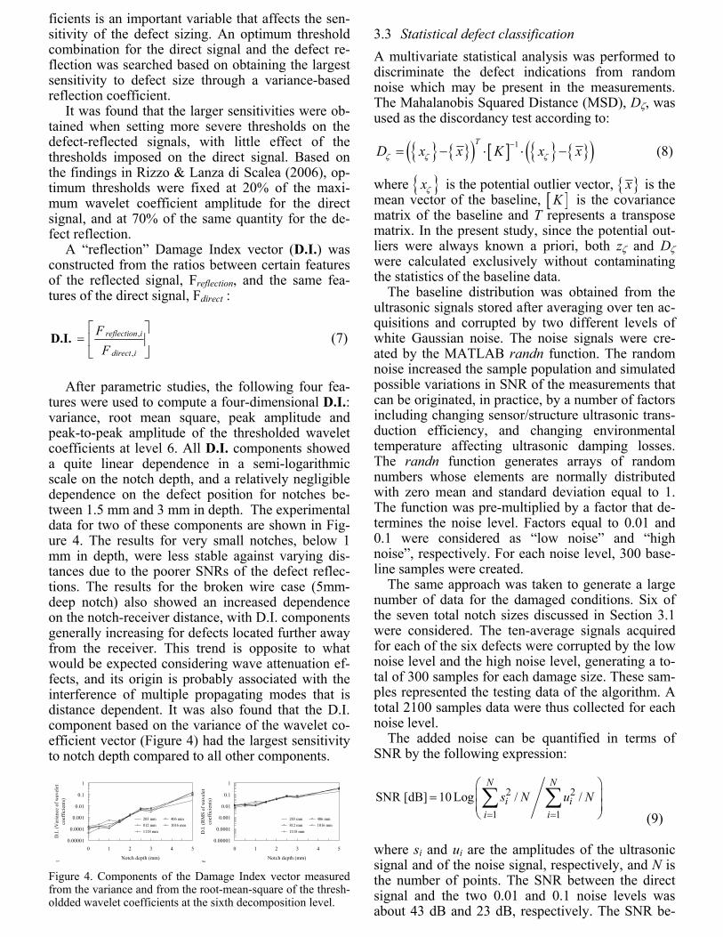
tures were used to compute a four-dimensional D.I.: variance, root mean square, peak amplitude and peak-to-peak amplitude of the thresholded wavelet coefficients at level 6. All D.I. components showed a quite linear dependence in a semi-logarithmic scale on the notch depth, and a relatively negligible dependence on the defect position for notches be-tween 1.5 mm and 3 mm in depth. The experimental data for two of these components are shown in Fig-ure 4. The results for very small notches, below 1 mm in depth, were less stable against varying dis-tances due to the poorer SNRs of the defect reflec-tions. The results for the broken wire case (5mm-deep notch) also showed an increased dependence on the notch-receiver distance, with D.I. components generally increasing for defects located further away from the receiver. This trend is opposite to what would be expected considering wave attenuation ef-fects, and its origin is probably associated with the interference of multiple propagating modes that is distance dependent. It was also found that the D.I. component based on the variance of the wavelet co-efficient vector (Figure 4) had the largest sensitivity to notch depth compared to all other components.

0.00001

0.0001

0.001

0.01

0.1

1

0 1 2 3 4 5

Notch depth (mm)

D.I.

(Var

ianc

e of

wav

elet

coef

ficie

nts)

203 mm 406 mm 812 mm 1016 mm 1118 mm

et

0.00001

0.0001

0.001

0.01

0.1

1

0 1 2 3 4 5

Notch depth (mm)

D.I.

(RM

S of

wav

elet

co

effic

ient

s)

203 mm 406 mm 812 mm 1016 mm 1118 mm

f Figure 4. Components of the Damage Index vector measured from the variance and from the root-mean-square of the thresh-oldded wavelet coefficients at the sixth decomposition level.

3.3 Statistical defect classification A multivariate statistical analysis was performed to discriminate the defect indications from random noise which may be present in the measurements. The Mahalanobis Squared Distance (MSD), Dζ, was used as the discordancy test according to:

{ } { }( ) [ ] { } { }( )1TD x x K x xζ ζ ζ

−= − ⋅ ⋅ − (8)

where { }xζ is the potential outlier vector, { }x is the mean vector of the baseline, [ ]K is the covariance matrix of the baseline and T represents a transpose matrix. In the present study, since the potential out-liers were always known a priori, both zζ and Dζ were calculated exclusively without contaminating the statistics of the baseline data.

The baseline distribution was obtained from the ultrasonic signals stored after averaging over ten ac-quisitions and corrupted by two different levels of white Gaussian noise. The noise signals were cre-ated by the MATLAB randn function. The random noise increased the sample population and simulated possible variations in SNR of the measurements that can be originated, in practice, by a number of factors including changing sensor/structure ultrasonic trans-duction efficiency, and changing environmental temperature affecting ultrasonic damping losses. The randn function generates arrays of random numbers whose elements are normally distributed with zero mean and standard deviation equal to 1. The function was pre-multiplied by a factor that de-termines the noise level. Factors equal to 0.01 and 0.1 were considered as “low noise” and “high noise”, respectively. For each noise level, 300 base-line samples were created.

The same approach was taken to generate a large number of data for the damaged conditions. Six of the seven total notch sizes discussed in Section 3.1 were considered. The ten-average signals acquired for each of the six defects were corrupted by the low noise level and the high noise level, generating a to-tal of 300 samples for each damage size. These sam-ples represented the testing data of the algorithm. A total 2100 samples data were thus collected for each noise level.

The added noise can be quantified in terms of SNR by the following expression:

2 2

1 1SNR [dB] 10 Log / /

N N

i ii i

s N u N= =

⎛ ⎞⎜ ⎟=⎜ ⎟⎝ ⎠∑ ∑

(9) where si and ui are the amplitudes of the ultrasonic signal and of the noise signal, respectively, and N is the number of points. The SNR between the direct signal and the two 0.01 and 0.1 noise levels was about 43 dB and 23 dB, respectively. The SNR be-

tween the reflection from the 3 mm-deep notch and the two 0.01 and 0.1 noise levels was about 32 dB and 12 dB, respectively. Clearly, the latter two val-ues decreased with decreasing notch depth.

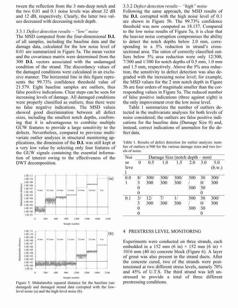
3.3.1 Defect detection results – “low” noise The MSD computed from the four-dimensional D.I. of all samples, including the baseline data and the damage data, calculated for the low noise level of 0.01 are summarized in Figure 5a. The mean vector and the covariance matrix were determined from the 300 D.I. vectors associated with the undamaged condition of the strand. The discordancy values of the damaged conditions were calculated in an exclu-sive manner. The horizontal line in this figure repre-sents the 99.73% confidence threshold value of 21.579. Eight baseline samples are outliers, thus false positive indications. Clear steps can be seen for increasing levels of damage. All damaged conditions were properly classified as outliers, thus there were no false negative indications. The MSD values showed good discrimination between all defect sizes, including the smallest notch depths, confirm-ing that it is advantageous to combine multiple GUW features to provide a large sensitivity to the defects. Nevertheless, compared to previous multi-variate outlier analyses in structural monitoring ap-plications, the dimension of the D.I. was still kept at a very low value by selecting only four features of the GUW signals containing the essential informa-tion of interest owing to the effectiveness of the DWT decomposition.

1.0E-011.0E+001.0E+011.0E+021.0E+031.0E+041.0E+051.0E+061.0E+071.0E+081.0E+091.0E+101.0E+11

0 300 600 900 1200 1500 1800 2100

Sample number

Mah

alan

obis

dis

tanc

e

1.0E-011.0E+001.0E+011.0E+021.0E+031.0E+041.0E+051.0E+061.0E+071.0E+081.0E+091.0E+101.0E+11

0 300 600 900 1200 1500 1800 2100

Sample number

Mah

alan

obis

dis

tanc

e

0 mm 0.5 mm 1.0 mm 1.5 mm 2.0 mm 3.0 mm b.w

0 mm 0.5 mm 1.0 mm 1.5 mm 2.0 mm 3.0 mm b.w

(b)

(a)

Figure 5. Mahalanobis squared distance for the baseline (un-damaged) and damaged strand data corrupted with the low-level noise (a) and the high-level noise (b).

3.3.2 Defect detection results – “high” noise Following the same approach, the MSD results of the D.I. corrupted with the high noise level of 0.1 are shown in Figure 5b. The 99.73% confidence threshold was now computed as 18.137. Compared to the low noise results of Figure 5a, it is clear that the heavier noise corruption compromises the ability to detect the notch depths below 2.0 mm, corre-sponding to a 5% reduction in strand’s cross-sectional area. The ratios of correctly classified out-liers below 5% area reduction were only 12/300, 7/300 and 1/300 for notch depths of 0.5 mm, 1.0 mm and 1.5 mm, respectively. Above the 5% area reduc-tion, the sensitivity to defect detection was also de-graded with the increasing noise level; for example, the MSD values for the 2 mm notch depth in Figure 5b are four orders of magnitude smaller than the cor-responding values in Figure 5a. The reduced number of false positive indications (three against eight) is the only improvement over the low noise level.

Table 1 summarizes the number of outliers de-tected in the multivariate analyses for both levels of noise considered; the outliers are false positive indi-cations for the baseline data (Damage Size 0) and, instead, correct indications of anomalies for the de-fect data.

Table 1. Results of defect detection for outlier analysis: num-ber of outliers n/300 for the various damage sizes and two lev-els of noise.

Damage Size (notch depth – mm) Noise level

0 0.5 1.0 1.5 2.0 3.0 5.0 (b.w.)

0.01

8/ 300

300/ 300

300/ 300

300/ 300

300/ 300

300/ 300

300/ 300

0.1 3/ 300

12/ 300

7/ 300

1/ 300

300/ 300

300/ 300

300/ 300

4 PRESTRESS LEVEL MONITORING

Experiments were conducted on three strands, each embedded in a 152 mm (6 in) × 152 mm (6 in) × 1016 mm (40 in) concrete block (Figure 6). A layer of grout was also present in the strand ducts. After the concrete cured, two of the strands were post-tensioned at two different stress levels, namely 70% and 45% of U.T.S. The third strand was left un-stressed to provide a total of three different prestressing conditions.

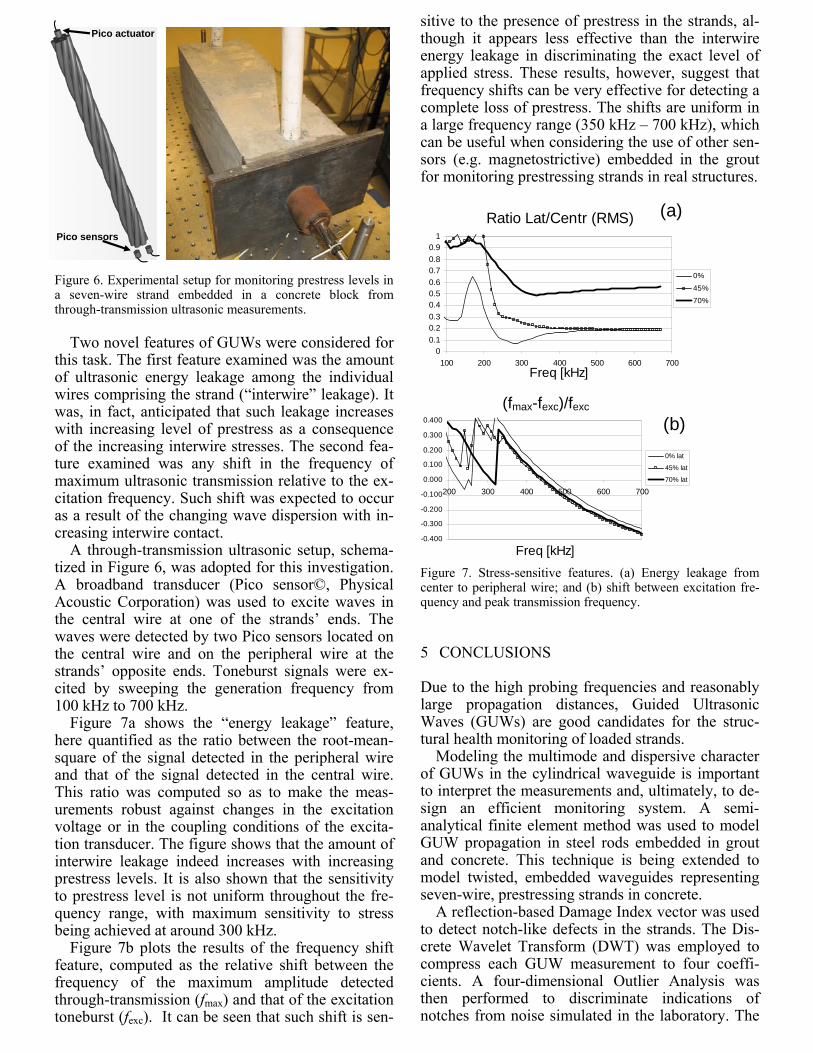
Figure 6. Experimental setup for monitoring prestress levels in a seven-wire strand embedded in a concrete block from through-transmission ultrasonic measurements.

Two novel features of GUWs were considered for this task. The first feature examined was the amount of ultrasonic energy leakage among the individual wires comprising the strand (“interwire” leakage). It was, in fact, anticipated that such leakage increases with increasing level of prestress as a consequence of the increasing interwire stresses. The second fea-ture examined was any shift in the frequency of maximum ultrasonic transmission relative to the ex-citation frequency. Such shift was expected to occur as a result of the changing wave dispersion with in-creasing interwire contact.

A through-transmission ultrasonic setup, schema-tized in Figure 6, was adopted for this investigation. A broadband transducer (Pico sensor©, Physical Acoustic Corporation) was used to excite waves in the central wire at one of the strands’ ends. The waves were detected by two Pico sensors located on the central wire and on the peripheral wire at the strands’ opposite ends. Toneburst signals were ex-cited by sweeping the generation frequency from 100 kHz to 700 kHz.

Figure 7a shows the “energy leakage” feature, here quantified as the ratio between the root-mean-square of the signal detected in the peripheral wire and that of the signal detected in the central wire. This ratio was computed so as to make the meas-urements robust against changes in the excitation voltage or in the coupling conditions of the excita-tion transducer. The figure shows that the amount of interwire leakage indeed increases with increasing prestress levels. It is also shown that the sensitivity to prestress level is not uniform throughout the fre-quency range, with maximum sensitivity to stress being achieved at around 300 kHz.

Figure 7b plots the results of the frequency shift feature, computed as the relative shift between the frequency of the maximum amplitude detected through-transmission (fmax) and that of the excitation toneburst (fexc). It can be seen that such shift is sen-

sitive to the presence of prestress in the strands, al-though it appears less effective than the interwire energy leakage in discriminating the exact level of applied stress. These results, however, suggest that frequency shifts can be very effective for detecting a complete loss of prestress. The shifts are uniform in a large frequency range (350 kHz – 700 kHz), which can be useful when considering the use of other sen-sors (e.g. magnetostrictive) embedded in the grout for monitoring prestressing strands in real structures.

Figure 7. Stress-sensitive features. (a) Energy leakage from center to peripheral wire; and (b) shift between excitation fre-quency and peak transmission frequency.

5 CONCLUSIONS

Due to the high probing frequencies and reasonably large propagation distances, Guided Ultrasonic Waves (GUWs) are good candidates for the struc-tural health monitoring of loaded strands. Modeling the multimode and dispersive character of GUWs in the cylindrical waveguide is important to interpret the measurements and, ultimately, to de-sign an efficient monitoring system. A semi-analytical finite element method was used to model GUW propagation in steel rods embedded in grout and concrete. This technique is being extended to model twisted, embedded waveguides representing seven-wire, prestressing strands in concrete.

A reflection-based Damage Index vector was used to detect notch-like defects in the strands. The Dis-crete Wavelet Transform (DWT) was employed to compress each GUW measurement to four coeffi-cients. A four-dimensional Outlier Analysis was then performed to discriminate indications of notches from noise simulated in the laboratory. The

Pico actuator

Pico sensors

(fexc-fmax)/fexc

-0.400

-0.300

-0.200

-0.100

0.000

0.100

0.200

0.300

0.400

200 300 400 500 600 700

Freq [kHz]

0% lat

45% lat

70% lat

Ratio Lat/Centr (RMS)

00.10.20.30.40.50.60.70.80.9

1

100 200 300 400 500 600 700Freq [kHz]

0%

45%70%

(a)

(b)(fmax-fexc)/fexc

notches considered were located as far away as 1,100 mm from the sensors. The algorithm was able to properly flag notches as small as 0.5 mm (0.7% strand’s area reduction) for SNRs on the order of 32 dB. For higher noise levels, corresponding to SNRs on the order of 12 dB, the properly flagged notches were as small as 2 mm (5% strand’s area reduction).

In a parallel study, through-transmission meas-urements were collected to identify wave features sensitive to prestress levels in strands embedded in post-tensioned concrete blocks. The amount of wave energy leakage between the central wire and the pe-ripheral wires was one stress-sensitive feature identi-fied. The shift between excitation frequency and peak transmission frequency was another stress-sensitive feature identified. Both of these features are being investigated further to assess their applica-bility to a monitoring system where sensors are em-bedded along the length of a strand in a real struc-ture.

ACKNOWLEDGMENTS

The strand monitoring project is funded at UCSD by the U.S. National Science Foundation under grant # 0221707 (Dr. S-C. Liu, Program Manager), and by the California Department of Transportation under contract # 59A0538 (Dr. C. Sikorsky, Program Manager). Funding was also provided by the Italian Ministry for University and Scientific & Technological Research MIUR (40%). The topic of research is part of the research thrusts of the Centre of Study and Research for the Identification of Materials and Structures (CIMEST) at the University of Bologna.

REFERENCES

Bartoli, I., Marzani, A., Lanza di Scalea, F. & Viola, E. 2006. Modeling wave propagation in damped waveguides of arbi-trary cross-section, Journal of Sound and Vibration, 295: 685-707.

Beard, M.D.; Lowe, M.J.S. & Cawley, P. 2003. Ultrasonic guided waves for inspection of grouted tendons and bolts. ASCE Journal of Materials in Civil Engineering, 15: 212-218.

Chase, S.B. 2001. Smarter bridges, why and how? Smart Mae-rials Bulletin, 2: 9-13.

Chen, H.-L. & Wissawapaisal, K. 2002. Application of Wigner-Ville transform to evaluate tensile forces in seven-wire prestressing strands. ASCE Journal of Materials in Civil Engineering, 128: 1206-1214.

Hayashi, T., Song, W.J. & Rose, J.L. 2003. Guided wave dis-persion curves for a bar with an arbitrary cross-section, a rod and rail example. Ultrasonics, 41: 175-183.

Huang, K.H. & Dong, S.B. 1984. Propagating waves and edge vibrations in anisotropic composite cylinders. Journal of Sound and Vibration, 96: 363-379.

Kwun, H. & Teller, C. M. 1994. Detection of fractured wires in steel cables using magnetostrictive sensors. Materials Evaluation, 503-507.

Kwun, H. & Teller, C.M. 1995. Nondestructive Evaluation of Steel Cables and Ropes Using Magnetostrictively Induced Ultrasonic Waves and Magnetostrictively Detected Acous-tic Emissions. U.S. Patent No. 5,456,113, 1995.

Kwun, H., Bartels, K.A. & Hanley, J.J. 1998. Effect of tensile loading on the properties of elastic-wave in a strand. Jour-nal of the Acoustical Society of America, 103: 3370-3375.

Lanza di Scalea, F., Rizzo, P. & Seible, F. 2003. Stress meas-urement and defect detection in steel strands by guided stress waves. ASCE Journal of Materials in Civil Engineer-ing, 15: 219-227.

Parker, D. 1996. Tropical overload. New Civil Engineer, 18-21. Pavlakovic, B.N., Lowe, M.J.S. & Cawley, P. 1999. The in-

spection of tendons in post-tensioned concrete using guided ultrasonic waves. Insight-NDT&Condition Monitoring, 41: 446-452.

Pavlakovic, B.N., Lowe, M.J.S. & Cawley, P. 2001. High-frequency low-loss ultrasonic modes in imbedded bars. Journal of Applied Mechanics, 68: 67-75.

Reis, H., Ervin, B.L., Kuchma, D.A. & Bernhard, J.T. 2005. Estimation of corrosion damage in steel reinforced mortar using guided waves. ASME Journal of Pressure Vessel Technology, 127: 255-261.

Rizzo, P. & Lanza di Scalea, F. 2001. Acoustic emission moni-toring of carbon-fiber-reinforced-polymer bridge stay ca-bles in large-scale testing. Experimental Mechanics, 41: 282-290.

Rizzo, P. & Lanza di Scalea, F. 2004. Wave propagation in multi-wire strands by wavelet-based laser ultrasound. Ex-perimental Mechanics, 44: 407-415.

Rizzo, P. & Lanza di Scalea, F. 2005. Ultrasonic inspection of multi-wire steel strands with the aid of the wavelet trans-form. Smart Materials and Structures, 14: 685-695.

Rizzo, P. & Lanza di Scalea, F. 2006. Discrete wavelet trans-form for enhancing defect detection in strands by guided ul-trasonic waves. International Journal of Structural Health Monitoring, 5: 297-308.

Washer, G., Green, R.E. & Pond, R.B. 2002. Velocity con-stants for ultrasonic stress measurements in prestressing tendons. Research in Nondestructive Evaluation, 14: 81-94.

Watson, S.C. & Stafford, D. 1988. Cables in Trouble. Civil Engineering, 58: 38-41.

Woodward, R.J. 1988. Collapse of Ynys-y-Gwas bridge, West Glamorgan. Proceedings of the Institution of Civil Engi-neers, 84: 635-669.