Structural Health Monitoring of Adhesively Bonded ... · Structural Health Monitoring of Adhesively...
212
Structural Health Monitoring of Adhesively Bonded Composite Joints By Fady Habib B.Eng A Thesis Submitted to The Faculty of Graduate Studies and Research In partial fulfilment of the degree requirements of Master of Applied Science Ottawa-Carleton Institute for Mechanical and Aerospace Engineering Department of Mechanical and Aerospace Engineering Carleton University Ottawa, Ontario, Canada January 2012 Copyright © 2012- Fady Habib
Transcript of Structural Health Monitoring of Adhesively Bonded ... · Structural Health Monitoring of Adhesively...

Structural Health Monitoring of Adhesively Bonded
Composite Joints
By
Fady Habib B.Eng
A Thesis Submitted to The Faculty of Graduate Studies and Research
In partial fulfilment of the degree requirements of Master of Applied Science
Ottawa-Carleton Institute for
Mechanical and Aerospace Engineering
Department of Mechanical and Aerospace Engineering
Carleton University Ottawa, Ontario, Canada
January 2012
Copyright ©
2012- Fady Habib

Library and Archives Canada
Published Heritage Branch
Bibliotheque et Archives Canada
Direction du Patrimoine de I'edition
395 Wellington Street Ottawa ON K1A0N4 Canada
395, rue Wellington Ottawa ON K1A 0N4 Canada
Your file Votre reference
ISBN: 978-0-494-91573-8
Our file Notre reference
ISBN: 978-0-494-91573-8
NOTICE:
The author has granted a nonexclusive license allowing Library and Archives Canada to reproduce, publish, archive, preserve, conserve, communicate to the public by telecommunication or on the Internet, loan, distrbute and sell theses worldwide, for commercial or noncommercial purposes, in microform, paper, electronic and/or any other formats.
AVIS:
L'auteur a accorde une licence non exclusive permettant a la Bibliotheque et Archives Canada de reproduire, publier, archiver, sauvegarder, conserver, transmettre au public par telecommunication ou par I'lnternet, preter, distribuer et vendre des theses partout dans le monde, a des fins commerciales ou autres, sur support microforme, papier, electronique et/ou autres formats.
The author retains copyright ownership and moral rights in this thesis. Neither the thesis nor substantial extracts from it may be printed or otherwise reproduced without the author's permission.
L'auteur conserve la propriete du droit d'auteur et des droits moraux qui protege cette these. Ni la these ni des extraits substantiels de celle-ci ne doivent etre imprimes ou autrement reproduits sans son autorisation.
In compliance with the Canadian Privacy Act some supporting forms may have been removed from this thesis.
While these forms may be included in the document page count, their removal does not represent any loss of content from the thesis.
Conformement a la loi canadienne sur la protection de la vie privee, quelques formulaires secondaires ont ete enleves de cette these.
Bien que ces formulaires aient inclus dans la pagination, il n'y aura aucun contenu manquant.
Canada

Abstract
In recent years, many aerospace organizations have researched and implemented composite
materials to achieve better fuel efficiency as well as reduced maintenance cost. In addition to
the use of composites, manufacturers are investigating the use of adhesive bonded joints and
composite patch bonded repairs to extend the life of their in-service aircraft. Adhesive joints are
superior to traditional mechanical fasteners as they reduce stress concentration zones and
overall part count. However, the integrity of an adhesive joint is difficult to inspect. Inspection
of adhesive joints may be carried out using interrogation technology such as Structural Health
Monitoring (SHM). This thesis focuses on the evaluation of Acoustic-Ultrasonic (AU) SHM
technique for the detection of crack and disbond growth. In addition to AU, Capacitance
Disbond Detection Technique (CDDT) and the Surface Mountable Crack Detection System
(SMCDS) were evaluated for the detection disbonds. Results of the AU system demonstrated
that AU technology may be used to detect and quantify crack and disbond growth. It was also
found that SMCDS and CDDT both complement each other, as SMCDS identified the location of
disbond while CDDT quantify disbond.
Structural-Health Monitoring of Adhesively Bonded Composite Joints Page ii

Acknowledgments During the course of my master's degree I have had the pleasure of working with many
knowledgeable individuals from both the National Research Council Canada (NRC) and Carleton
University. I would like to thank all of them for their guidance, support and their patience. In the
event that I forget to mention your name below, I truly apologize. Before I begin to thank all the
individuals I have worked with over these years, I would like to start by thanking those who have
always been there for me since my birth; My Family.
Of all the individuals I have worked with, I would like to thank both my supervisors: Prof.
Martinez and Prof. Artemev for providing me with guidance and knowledge. I would mostly like
to thank them for spending a great deal of time reviewing my 200 page thesis; I know it wasn't
easy. Prof.+ Martinez was unlike any professor that I have ever had. He was not just my
supervisor for these past two years but was also a good friend.
I would like to extend my thanks to: Tom Benak, Tom Kay, Brian Moyes, Mike Brothers, Marc
Genest, and Michel Delannoy for their aid in manufacturing and testing of all my coupons. I
would also like to thank Dr. Guillaume Renaud for his AFGROW analysis that he conducted for
me.
I would also like to thank two of my closest friends Mario and Shashank for their friendship over
this past little while. The part I regret the most during my academic career was, not knowing you
guys during my undergrad years. We have spent many hours discussing academia, research and
life objects over coffee, food and sometimes beer. I think that if we add up all our individual
hours spent together, it would probably add up to how much time a person takes to finish a
Ph.D. Also, thank you Shashank for spending time with me to explain Lamb Wave theory.
Structural Health Monitoring of Adhesively Bonded Composite Joints Page iii

For financial support, I would like to thank NRC, Carleton University and MITACS. All of their
funding has played an important role in the testing of advanced SHM technologies. More
importantly, it has helped me expand my knowledge and personal growth.
Structural Health Monitoring of Adhesively Bonded Composite Joints Page iv

Table of Contents
Abstract ii
Acknowledgments iii
Table of Contents v A
List of Tables ix
List of Figures x
List of Equations xv
Abbreviations xvii
Nomenclature xviii
Preface 1
1.0 Chapter 1.0: Literature Review 2
1.1 Introduction to Composites 3
1.1.1 Applications of Composites 4
1.1.1.1 Aerospace Composite Application 5
1.1.1.2 Other Composite Applications 7
1.1.2 Basics of Composites 8
1.1.3 Joining of Composite Materials 9
1.1.3.1 Patch Bonded Repairs 11
1.2 Inspection of Structures 14
1.2.1 Non-Destructive Evaluations (NDE) 15
1.2.1.1 Visual Inspection 16
1.2.1.2 Ultrasound 17
1.2.1.3 Eddy Current 19
1.2.1.4 Acoustic Emission 20
1.2.1.5 X-Ray Radiography 20
1.2.1.6 Thermography 21
1.2.2 Structural Health Monitoring (SHM) 22
1.2.2.1 Fibre Bragg Gratings (FBG) 24
1.2.2.2 Strain Gauges (SG) 26
1.2.2.3 Eddy Current 26
1.2.2.4 Capacitance Disbond Detection Technique (CDDT) 27
Structural Health Monitoring of Adhesively Bonded Composite Joints Page v

1.2.2.5 Comparative Vacuum Monitoring (CVM) 28
1.2.2.6 Surface Mountable Crack Detection System (SMCDS) 29
1.2.2.7 Acousto-Ultrasonic (AU) 30
1.2.2.8 Acoustic Emission (AE) 30
1.3 Inspection of Patch Repairs 31
1.4 Conclusion 34
2.0 Chapter 2.0: Selection of Damage Detection Systems 36
2.1 Non-Destructive Evaluation (NDE) Systems 36
2.1.1 Ultrasound Inspection 36
2.1.2 Thermography 40
2.2 Structural Health Monitoring (SHM) Systems 45
2.2.1 Capacitance Disbond Detection Technique (CDDT) 47
2.2.1.1 Basics of a capacitor 47
2.2.2 Surface Mountable Crack Detection System (SMCDS) 49
2.2.2.1 Basics of Surface Mountable Crack Sensors (SMCS) 50
2.2.3 Acousto-Ultrasonic (AU) 52
2.2.3.1 Basics of Lamb waves 53
2.2.3.1.1 Symmetric and anti-symmetric solutions 61
2.2.3.1.2 Numerical solution to Lamb wave equations 63
2.2.3.2 Analysis of Lamb waves 64
2.2.3.2.1 Time Domain (TD) analysis 65
2.2.3.3 The Acellent system 69
2.2.3.3.1 SmartPatch* application setup 70
2.2.3.3.2 The Acellent system analysis 75
3.0 Chapter 3.0: Test Design and Coupon Manufacturing 78
3.1 Coupons 78
3.1.1 Metallic Coupons (Coupon Set 1) 79
3.1.2 Patched Metallic Coupons (Coupon Set 2) 81
3.1.3 Composite-to-Composite Coupons (Coupon Set 3) 82
3.1.3.1 Coupon design requirements 83
3.1.3.2 Material properties 84
3.1.3.3 Finite Element Analysis (FEA) 85
Structural Health Monitoring of Adhesively Bonded Composite Joints Page vi

3.1.3.3.1 Conventional shell model (Model 1) 90
3.1.3.3.1.1 Variant patch designs and analysis 95
3.1.3.3.1.2 Variant patch geometry and analysis 96
3.1.3.3.1.3 Variant ply orientation analysis 97
3.1.3.3.1.4 Summary of results 98
3.1.3.3.2 Continuum shell model (Model 2) 99
3.1.3.3.2.1 Results 100
3.1.3.3.3 Solid model (Model 3) 101
3.1.3.3.34 Results 102
3.1.3.4 Carbon fibre substrate manufacturing 107
3.1.3.4.1 CYCOM 5276-1G40-800 prepreg tape cutting 107
3.1.3.4.2 Laminate bagging Ill
3.1.3.4.3 Laminate curing 113
3.1.3.4.4 Laminate manufacturing results 114
3.1.3.5 Patch manufacturing 116
3.1.3.5.1 Patch bagging (Trial 1) 117
3.1.3.5.2 Patch curing (Trial 1) 118
3.1.3.5.3 Patch manufacturing results (Trial 1) 119
3.1.3.5.4 Patch manufacturing (Trial 2) 120
3.1.3.5.5 Patch bagging (Trial 2) 121
3.1.3.5.6 Patch curing (Trial 2) 122
3.1.3.5.7 Patch results (Trial 2) 122
3.1.3.6 Patch to substrate bonding 123
3.1.3.6.1 Bonding setup 123
3.1.3.6.2 Coupon (final assembly) bagging 125
3.1.3.6.3 Bonding curing 126
3.1.3.6.4 Bonding results 127
3.1.3.7 Coupon instrumentation 128
3.1.3.7.1 Acousto-Ultrasonic sensors 129
3.1.3.7.2 Capacitance Disbond Detection Technique (CDDT) sensors 131
3.1.3.7.3 Surface Mountable Crack Detection System (SMCDS) 132
3.2 Conclusion 134
Structural Health Monitoring of Adhesively Bonded Composite Joints Page vii
4.0 Chapter 4.0: Testing and Results 137
4.1 Metallic Coupon (Set 1) 139
4.1.1 Apparatus Setup 139
4.1.2 Software Setup 140
4.1.3 Results 142
4.1.3.1 Direct Path Image (DPI) utility results 143
4.1.3.2 Semi Empirical Damage Sizing (SEDS) results 146
4.2 Composite to Metallic (Coupon Set 2) 150
4.2.1 Apparatus Setup 150
4.2.2 Results 151
4.2.2.1 Direct Path Image (DPI) utility results 152
4.2.2.2 Semi Empirical Damage Sizing (SEDS) Results 162
4.3 Composite-to-Composite (Set 3) 165
4.3.1 Apparatus Setu p 166
4.3.2 Results 167
4.3.2.1 Direct Path Image (DPI) utility results 170
4.3.2.2 Semi Empirical Damage Sizing (SEDS) results 173
4.3.2.3 Capacitance Disbond Detection Technique (CDDT) results 177
4.3.2.4 Surface Mountable Crack Detection System (SMCDS) results 181
5.0 Chapter 5.0: Conclusions 184
6.0 References 188
Structural Health Monitoring of Adhesively Bonded Composite Joints Page viii

List of Tables
Table 1: Coupon Design Requirements 83
Table 2: Material Properties 85
Table 3: Von Mises Stress Comparison 96
Table 4: Debulking Procedure Ill
Table 5: Bonding Debulking Procedure 125
Struaural Health Monitoring of Adhesively Bonded Composite Joints Page ix
List of Figures
Figure 1: Fully Articulated Helicopter Rotor Hub: (a) All-Composite Hub; (b) Metallic Hub [9] 4
Figure 2: Utilization of Composites across the United States [10] 4
Figure 3: Composites Utilization within Military Application (Northrop Grumman B-2 bomber)
[11] 6 Figure 4: Composites Utilization within Commercial Application (Airbus A320) [11] 6
Figure 5: Composites Utilization within Combat Aircraft [11] 7
Figure 6: Automotive Composites: (a) Aston Martin One-77 [14]; (b) Aston Martin One-77 Cross-
Section [15] 8
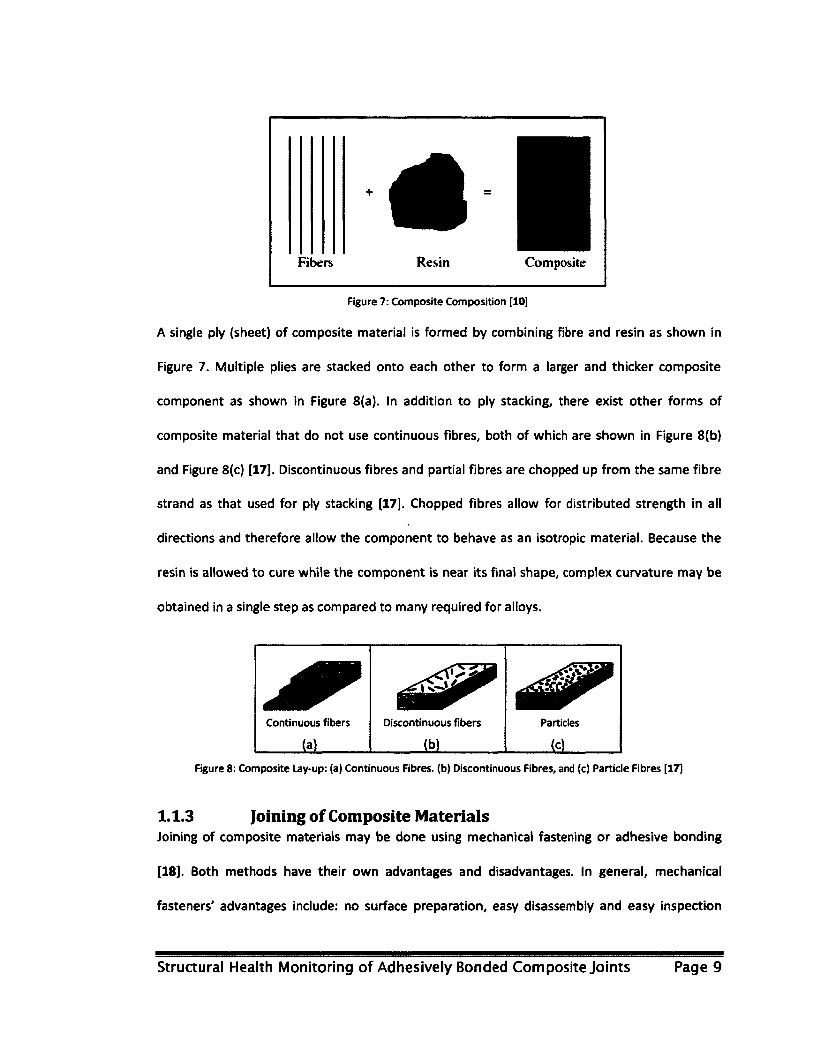
Figure 7: Composite Composition [10] 9
Figure 8: Composite Lay-up: (a) Continuous Fibres, (b) Discontinuous Fibres, and (c) Particle
Fibres [17] 9
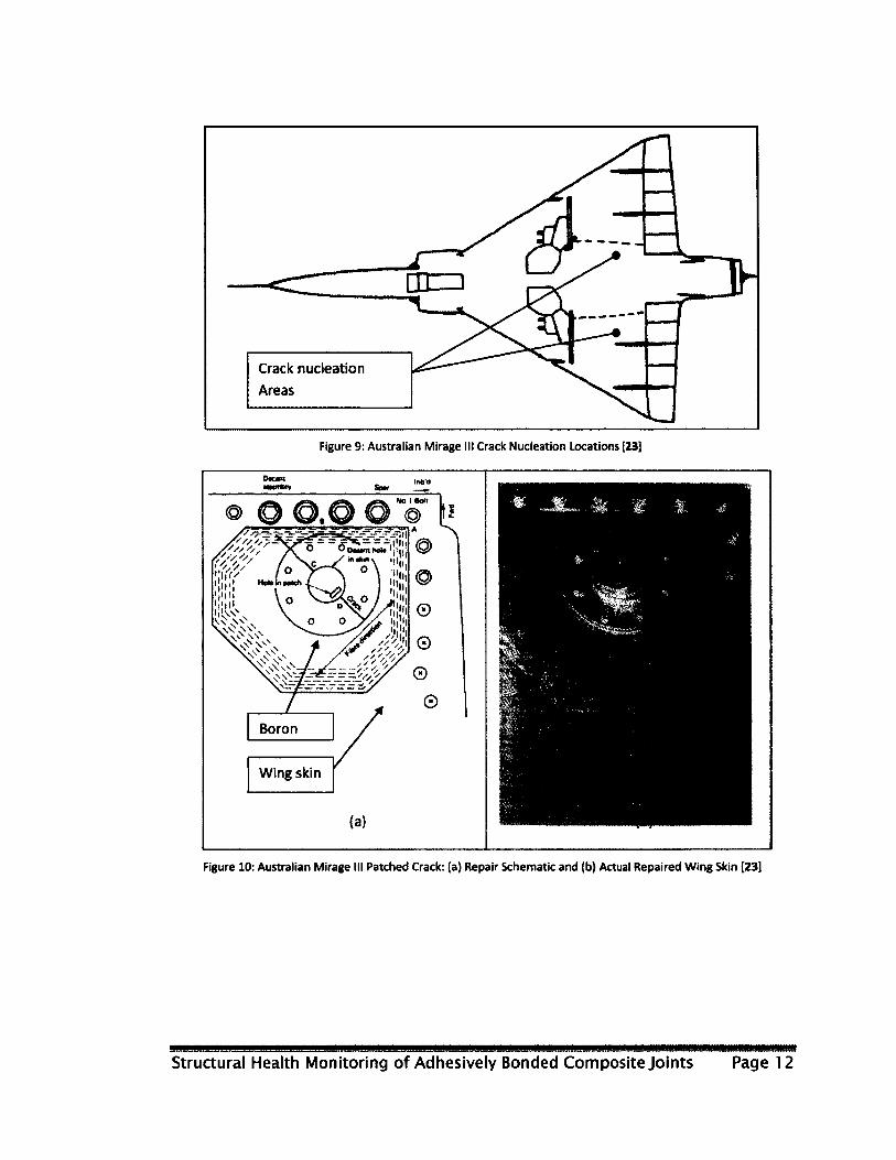
Figure 9: Australian Mirage III Crack Nucleation Locations [23] 12
Figure 10: Australian Mirage III Patched Crack: (a) Repair Schematic and (b) Actual Repaired
Wing Skin [23] 12
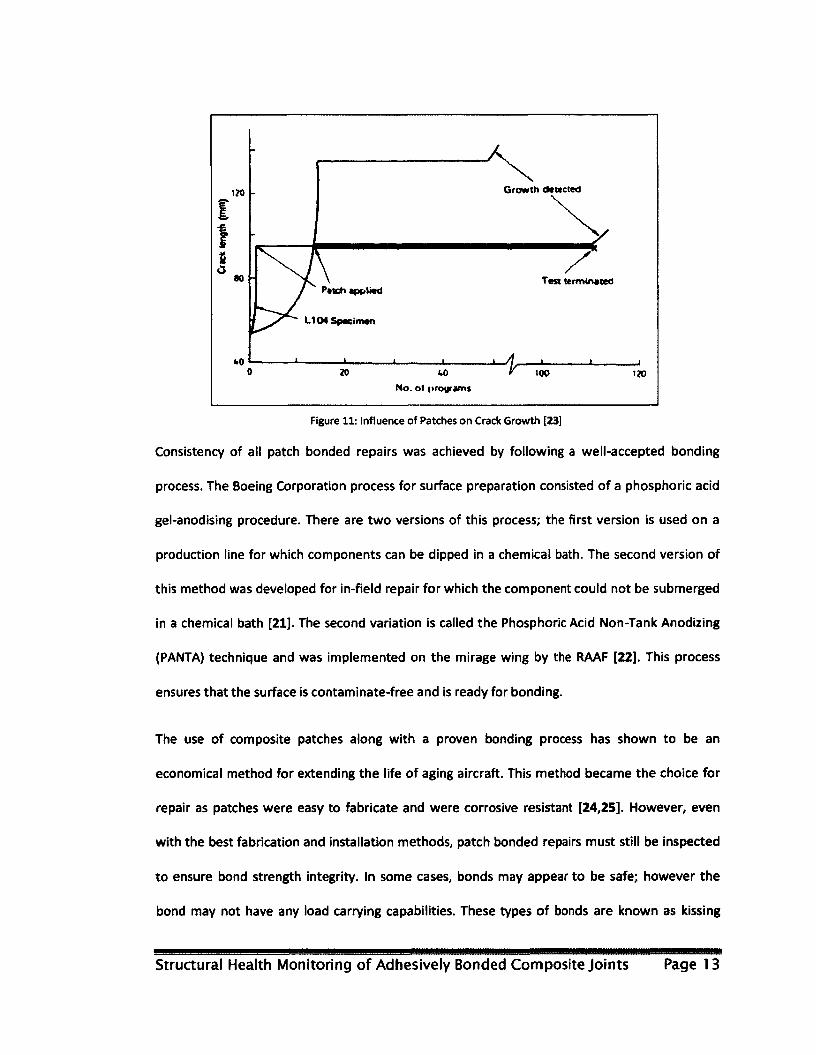
Figure 11: Influence of Patches on Crack Growth [23] 13
Figure 12: National Research Council Canada Holistic Structural Integrity Program 15
Figure 13: Point Analysis using A-Scan 18
Figure 14: Ultrasonic Signal of Pulse-Echo [32] 18
Figure 15: Eddy Current NDE [30] 19
Figure 16: Radiography [32] 21
Figure 17: Thermography [32] 22
Figure 18: Aircraft Nervous System [30,31] 23
Figure 19: Fibre Bragg Gratings [36] 25
Figure 20: Strain Gauge and Circuit: (a) Typical Strain Gauge; (b) Typical Quarter Bridge Circuit
[37] 26
Figure 21: Typical Eddy Current Sensor [30] 27
Figure 22: Capacitance Disbond Detection Technique: (a) Bonded Component; (b) Disbonded
Component 28
Figure 23: CVM Sensor [30] 29
Figure 24: SMCS Sensor 29
Figure 25: Acousto-Ultrasonic: (a) Sensor, Upper Side; (b) Sensor, Lower Side (Bond Surface); (c)
Data Acquisition [42] 30
Figure 26: Simulated Patched Coupons: left displays a non-cracked coupon while the right is a
cracked coupon [46] 32
Figure 27: FEA Results for Patch Repaired Coupons [46] 32
Figure 28: C-Scan of Patch [26] 33
Figure 29: Ultrasonic Inspection using Pulse-Echo: (a) Component with Flaw and (b) Signal
Results 37
Figure 30: A-Scan of a Component with Damage 38
Figure 31: B-Scan of a Component with Damage 39
Structural Health Monitoring of Adhesively Bonded Composite Joints Page x
Figure 32: C-Scan of a Component with Damage 40
Figure 33: Pulsed Thermography Setup 41
Figure 34: Pulsed Thermography Wave Propagation 41
Figure 35: Heat Wave Propagation: (a) Pulsed Thermography, and (b) Lock-in Thermography [54]
43
Figure 36: Temperature Profiles [54] 43
Figure 37: Example Thermography Images: (a) surface Thermal image after settling of
temperature, and (b) Thermal image with uneven heating on [54] 44
Figure 38: Pulsed Thermography: (a) Pulse within time domain, and (b) Pulse within frequency
domain [54] 45
Figure 39: Basics of a Capacitor 48
Figure 40: Patch Capacitor 49
Figure 41: SMCS Circuits: (a) Intact SMCS acting as a closed switch and (b) cracked SMCS acting
as an open switch 50
Figure 42: SMCS Composition 51
Figure 43: SMCS Placement 52
Figure 44: Co-ordinate System [33] 53
Figure 45: Particle Motion within a Solid Medium: (a) particles subject to pressure force, and (b)
particles subject to shear force [64] 54
Figure 46: Stress Distribution on a Small Element 57
Figure 47: Lamb Wave Propagation: (a) Symmetric mode and (b) Anti-symmetric mode 61
Figure 48: Dispersion Curves for Aluminum [63] 64
Figure 49: Lamb wave analysis of an aluminum plate: (a) Lamb waves and (b) Hilbert transform
[32] 66
Figure 50: Correlation of benchmark and damaged plate: (a) Lamb waves signal of a benchmark
composite plate, (b) Lamb waves of a damaged composite plate, (c) correlation
coefficient plot, and (d) the ratio between both correlation coefficients [32] 67
Figure 51: Signal Scatter due to the Presence of Damage [32] 69
Figure 52: Acellent Sensor Setup: (a) sensor creation and (b) sensor setup 71
Figure 53: Smart Layers: (a) single layer and (b) two smart layers 71
Figure 54: DAQ Setup 72
Figure 55: Path Definition: (a) path definition management, (b) path initiation and properties
and (c) path frequencies 73
Figure 56: Signal Propagation Settings 74
Figure 57: SmartPatch* Main Window 74
Figure 58: Direct Path Image Analysis 76
Figure 59: Semi-Empirical Input 77
Figure 60: Semi-Empirical Output 77
Figure 61: Aluminum Coupon with EDM Notch 80
Figure 62: Aluminum Coupon Crack Growth: (a) Fatigued coupon with rib, (b) Fatigued coupon
removed rib and (c) SMCS instrumented coupon prior to rib removal 80
Figure 63: Smart Patch Composite-Metallic Coupon Design: (a) Substrate and (b) Patch 82
Structural Health Monitoring of Adhesively Bonded Composite Joints Page xi
Figure 64: Common Stress Node 87
Figure 65: Conventional Shell Element Mesh Dependence Analysis 88
Figure 66: Continuum Shell Element Mesh Dependence Analysis 89
Figure 67:3D Stress Element Mesh Dependence Analysis 89
Figure 68: Smart Patch Phase 1 & 2 Coupon Design (measurements in inches) 90
Figure 69: Patch Part: (a) Spike Patch, (b) Chamfer Patch and (c) Unsymmetrical Spike Patch....91
Figure 70: Adhesive Part: (a) Adhesive for Patch 1, (b) Adhesive for Patch 2 and (c) Adhesive for
Patch 3 92
Figure 71: Substrate Part: (a) Dissections to Accommodate Patch 1, (b) Dissections to
Accommodate Patch 2 and (c) Dissections to Accommodate Patch 3 93
Figure 72: Assembly Position Constraints: (a) Isotropic View and (b) Side, Exploded View 94
Figure 73: Loads and Boundary Conditions: (a) Model 1, (b) Model 2 and (c) Model 3 95
Figure 74: Von Mises Adhesive Results: (a) Spike Patch, (b) Chamfer Patch and (c) Unsymmetrical
Spike Patch 96
Figure 75: Effects of Spike Angle on the S12 Adhesive Stresses 97
Figure 76: Effects of Ply Angle on S12 98
Figure 77: Mesh Sweep Direction 100
Figure 78: Comparison of both Continuum and Conventional Shell Models 101
Figure 79: Full Model Stresses 104
Figure 80: Stresses Distribution: (a) Patch, (b) Adhesive and (c) Magnified Adhesive 105
Figure 81: Change in Stress over Application of Heat and Load 106
Figure 82: Laminate-Substrate Schematics 108
Figure 83: Ply Cutting Procedure: (a) Carbon Fibre Roll, (b) 45° Alignment, (c) Straight Edge, and
(d) Ply Cuts 109
Figure 84: Layup Procedure: (a) Layup, and (b) Entrapped Air Removal 110
Figure 85: Layup Bagging: (a) Laminate Placement, (b) Covering of Laminate, (c) Breather Cloth,
and (d) Pulled Vacuum 113
Figure 86: CYCOM 5276-1 Temperature and Pressure Profiles 114
Figure 87: As Manufactured Carbon Fibre Laminates 115
Figure 88: Laminate Thickness Measurements 115
Figure 89: Patch and Laminate Geometry 116
Figure 90: Patch Bagging 118
Figure 91: Specialty Materials 5521F Boron Prepreg Tape Temperature and Pressure Profiles 119
Figure 92: Boron Patch Distortion 120
Figure 93: Patch Manufacturing Trial 2: (a) Patches with Tape Edge Dams, (b) Patches with
Surrounding Peel Ply 121
Figure 94: Patch Bagging Trial 2: (a) Patches with Tape Edge Dams, (b) Patches with Surrounding
Peel Ply 122
Figure 95: Patch Results Trial 2: (a) Patch with Tape Edge Dams and Surrounding Shims, (b) Patch
with Tape Edge Dams and No Surrounding Shims, (c) Patch with Surrounding Peel Ply
and Surrounding Shims and (d) Patch with Surrounding Peel Ply and No Surrounding
Shims 123
Structural Health Monitoring of Adhesively Bonded Composite Joints Page xii
Figure 96: Bonding Procedure: (a) Surface Preparation, (b) Patch to Substrate Alignment and (c)
Entrapped Air Removal 124
Figure 97: Bonding Bagging: (a) Coupon Wrapping, (b) Coupon Placement (c) Applying Vacuum
126
Figure 98: Cytec FM73 Film Adhesive Cure Profile 126
Figure 99: As Manufactured Coupon 128
Figure 100: Coupon Ultrasound C-Scan Inspections 128
Figure 101: Acellent Piezoelectric Sensors 129
Figure 102: Piezoelectric Sensors Layout: (a) Sensor layout 1, (b) Sensor layout 2 and (c) Sensor
scanning paths 130
Figure 103: Instrumented Coupon 131
Figure 104: CDDT Sensor 132
Figure 105: SMCDS: (a) insulating layer installation, (b) Insulating layer, (c) conductive layer
installation and (d) completed SMCS 133
Figure 106: SMCD Acquisition Module 134
Figure 107: Coupon Sailures: (a) Coupon Set 1 Fracture and (b) coupon Set 2 disbond and
fracture 138
Figure 108: Experimental Setup for Coupon Set 1 140
Figure 109: Coupon: (a) Actual coupon and (b) SmartPatch® coupon digital mapping
representation 141
Figure 110: Signal Propagation Settings 142
Figure 111: Damage Spectrum 145
Figure 112: Coupon SPP2-12 Direct Path Image Results at a 0.5 Threshold 145
Figure 113: Coupon SPP2-15 Direct Path Image Results at a 0.5 Threshold 145
Figure 114: Semi-Empirical Interpretations for Coupon SPP2-12 148
Figure 115: Semi-Empirical Interpretations for Coupon SPP2-15 148
Figure 116: Semi-Empirical Interpretations for Coupon SPP2-26 149
Figure 117: Experimental Setup for Coupon Set 2 151
Figure 118: Estimated Disbond Areas using Thermography 152
Figure 119: SPP2-11 Scanning Zones: (a) Zone 1, (b) Zone 2 and (c) Zone 3 153
Figure 120: Coupon SPP2-11: (a) DPI for all zones at a 0.5 threshold, (b) DPI for zone 1 at a 0.5
threshold, (c) DPI for zone 2 at a 0.5 threshold and (d) Thermography images 155
Figure 121: Coupon Scanning Zones: (a) SPP2-13 zones, (b) SPP2-14 and SPP2-18 scanning zones
157
Figure 122: Coupon SPP2-13: (a) DPI for all zones at a 0.5 threshold, (b) DPI for zone 1 at a 0.5
threshold, (c) DPI for zone 2 & 3 at a 0.5 threshold, (d) DPI for zone 4 at a 0.5 threshold
and (e) Thermography images 158
Figure 123: Coupon SPP2-14: (a) DPI for all zones, (b) DPI for zone 1, (c) DPI for zone 2 and (d)
Thermography images 161
Figure 124: Coupon SPP2-11 Semi-Empirical Interpretations 163
Figure 125: Semi-Empirical Interpretations for Coupon SPP2-13 164
Figure 126: Semi-Empirical Interpretations for Coupon SPP2-14 165
Structural Health Monitoring of Adhesively Bonded Composite Joints Page xiii
Figure 127: Disbond Area Estimations: (a) Coupon, (b) Adhesive cracking and (c) Estimated area
167
Figure 128: Sensor disbond 169
Figure 129: Signal Change due to Sensor Sisbond: (a) Signal path and (b) Signal change due to
sensor disbond 169
Figure 130: Sensor Configuration Modification 170
Figure 131: Coupon SPP3-04: (a) DPI utility results at 05 threshold and (b) Estimated disbond
areas 172
Figure 132: Coupon SPP3-12: (a) DPI utility results at 0.5 threshold and (b) Estimated disbond
areas 173
Figure 133: Semi-Empirical Interpretations for Coupon SPP3-04 175
Figure 134: Semi-Empirical Interpretations for Coupon SPP3-4a 176
Figure 135: Semi-Empirical Interpretations for Coupon SPP3-12 177
Figure 136: SPP3-16 Disbond Area Comparison to Capacitance Drop 178
Figure 137: SPP3-12 Disbond Area Comparison to Capacitance Drop 179
Figure 138: SPP3-16 Normalized Disbond Area Comparison to Capacitance Drop 180
Figure 139: SPP3-12 Normalized Disbond Area Comparison to Capacitance Drop 180
Figure 140: SPP3-04 SMCS Placement along Patch Edge 182
Figure 141: SPP3-04 SMCS Breakage 183
Figure 142: SPP3-4a SMCS Breakage at High Cycles 183
Structural Health Monitoring of Adhesively Bonded Composite Joints Page xiv

List of Equations
Equation 1 25
Equation 2 28
Equation 3 47
Equation 4 47
Equation 5 54
Equation 6 55
Equation 7 55
Equation 8 55
Equation 9 55
Equation 10 56
Equation 11 56
Equation 12 57
Equation 13 57
Equation 14 58
Equation 15 58
Equation 16 58
Equation 17 58
Equation 18 58
Equation 19 58
Equation 20 59
Equation 21 59
Equation 22 59
Equation 23 59
Equation 24 59
Equation 25 60
Equation 26 60
Equation 27 60
Equation 28 60
Equation 29 60
Equation 30 60
Equation 31 60
Equation 32 60
Equation 33 61
Equation 34 61
Equation 35 62
Equation 36 62
Equation 37 62
Equation 38 62
Equation 39 62
Equation 40 62
Structural Health Monitoring of Adhesively Bonded Composite Joints Page xv

Equation 41 62
Equation 42 62
Equation 43 62
Equation 44 62
Equation 45 63
Equation 46 63
Equation 47 63
Equation 48 66
Equation 49 68
Structural Health Monitoring of Adhesively Bonded Composite Joints Page xvi
Abbreviations Abbreviation Description AE Acoustic Emission AFGROW Air Force Growth AU Acousto-Ultrasonic CDDT Capacitance Disbond Detection Technique CFRP Carbon Fibre Reinforced Polymer CVM Comparative Vacuum Monitoring DAQ Data Acquisition DFT Discrete Fourier Transforms Dl Damage Index DPI Direct Path Image DSP Digital Signal Processing FBG Fibre Bragg Grating FEA Finite Element Analysis LT Lock in Thermography LW Lamb Wave MTS Material Test Frame NDE Non-Destructive Evaluation NRC National Research Council Canada PANTA Phosphoric Acid Non-Tank Anodizing PPT Pulsed Phase Thermography PT Pulsed Thermography PZT Lead Zirconate Titanate RAAF Royal Australian Air Force SEDS Semi-Empirical Damage Sizing SG Strain Gauge SHM Structural Health Monitoring SMCDS Surface Mountable Crack Detection System SMCS Surface Mountable Crack Sensor TD Time Domain ToF Time of Flight UT Ultrasound Inspection
Struaural Health Monitoring of Adhesively Bonded Composite Joints Page xvii
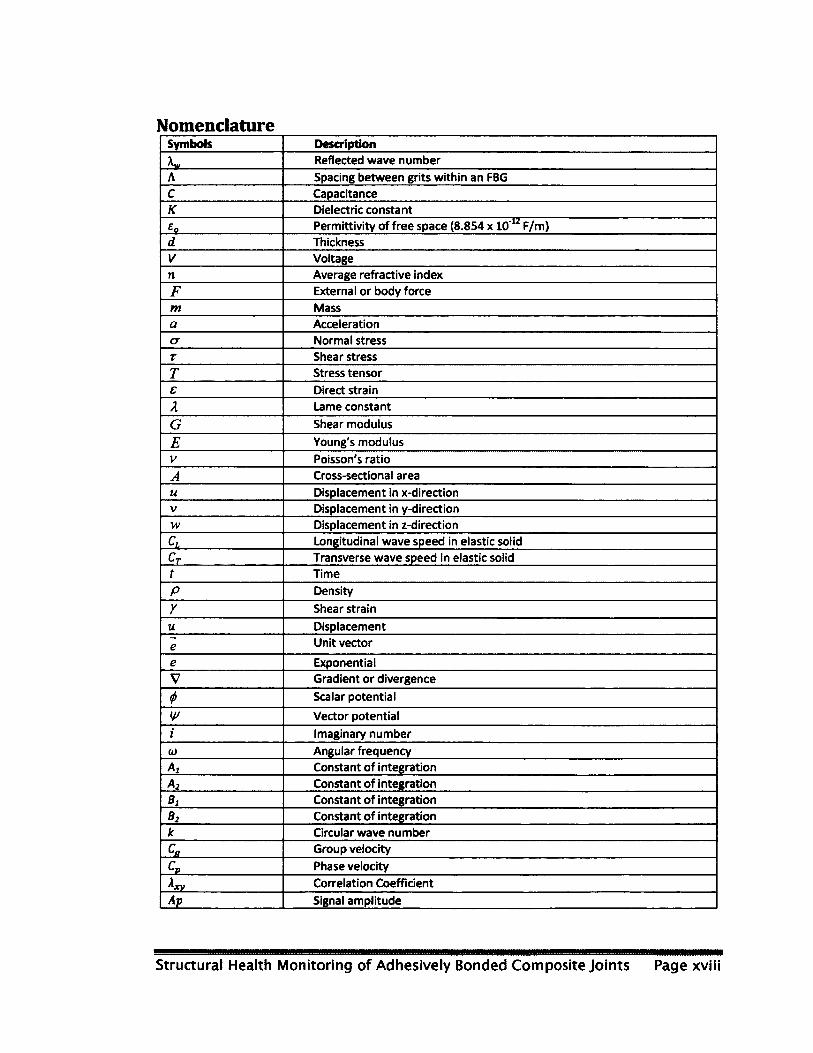
Nomenclature Symbols Description
Kv Reflected wave number A Spacing between grits within an FBG c Capacitance K Dielectric constant
Permittivity of free space (8.854 x 10"1Z F/m) d Thickness V Voltage n Average refractive index F External or body force m Mass a Acceleration a Normal stress X Shear stress T Stress tensor s Direct strain A Lame constant
G Shear modulus
E Young's modulus V Poisson's ratio A Cross-sectional area u Displacement in x-direction V Displacement in y-direction w Displacement in z-direction CL Longitudinal wave speed in elastic solid Cf Transverse wave speed in elastic solid t Time P Density
Y Shear strain u Displacement
e Unit vector
e Exponential V Gradient or divergence
Scalar potential
V Vector potential i Imaginary number 0) Angular frequency A, Constant of integration A2 Constant of integration BI Constant of integration B2 Constant of integration k Circular wave number ca Group velocity cv Phase velocity
A-XV Correlation Coefficient Ap Signal amplitude
Structural Health Monitoring of Adhesively Bonded Composite Joints Page xviii

Preface
Aviation advancements have been on the rise since the Wright brothers took the first ever
powered flight in late 1903. Since that remarkable day, military aircraft have far advanced to
incorporate both agility and stealth, while civilian aircraft have advanced in both efficiency and
safety. In recent years, both civilian and military requirements have been increasingly satisfied
through the use of advanced materials such as composites. However, composite materials have
many uncertainties as it relates to aging under operational environments. Unlike traditional
metallic materials, composites are susceptible to many forms of damage that are not visible to
the naked eye. These damages are a safety concern when left unrepaired, especially as aircraft
age.
Many in-service civilian and military aircraft today have well exceeded their design life.
However, airlines have made economic decisions to maintain and overhaul these aircraft rather
than purchasing new models for their fleet. Aging aircraft as well as new aircraft must be either
inspected by a mechanic or by an automated system. Inspections by aircraft mechanics require
removal of the aircraft from service which results in loss of profit for the airline. Automated
inspection systems may be a solution to eliminating the need to remove the aircraft from
service. These automated inspection systems are known as Structural Health Monitoring (SHM)
systems. SHM systems may be used on composite and metallic materials to determine the
initiation and growth of damage.
This research is focused on the evaluation of SHM systems for their effectiveness in damage
detection and quantification of failure within both metallic-to-composite and composite-to-
composite adhesive joints.
Structural Health Monitoring of Adhesively Bonded Composite Joints Page 1

Chapter 1.0: Literature Review
Composite materials have a variety of applications ranging from fashionable rings to turbine fan
blades. These materials are composed of reinforcing fibres and resin matrix. Fibres provide the
load carrying capability while the resin acts as a load transfer medium. Various combinations of
these two materials allow for different strength and therefore make composites very tailorable
for specific applications. Tailoring of composites does not end at component curing, rather at
the time an assembly is complete. Assemblies composed of two or more composite components
may be joined through the use of adhesives. Adhesives provide an optimal stress distribution as
compared to mechanical fasteners. However, unlike mechanical fasteners, adhesive joints are
not easily inspectable as the joint does not allow for disassembly.
The integrity of adhesive joints may be inspected through routine maintenance using Non-
Destructive Evaluations (NDE) or through the use of Structural Health Monitoring (SHM)
systems. There are many SHM system technologies that exist today, many of which are sold as
out-of-the-box solutions which are ready for integration and interrogation of structural
components. However, not all of these systems are effective and only a few are currently under
evaluation for certification on commercial aircraft [1,2]. In this research, several SHM systems
will be evaluated for the detection of crack growth and disbond.
This chapter provides necessary background required for understanding composites, adhesive
joints, NDE and SHM technologies.
Structural Health Monitoring of Adhesively Bonded Composite Joints Page 2

1.1 Introduction to Composites
Current advancements in materials science have led to increased use of advanced materials in
aircraft, automotive and civil structures. Advanced materials such as carbon fibre reinforced
polymers (CFRP) are composed of 2 phases: the fibre (reinforcement) and the matrix (load
transfer medium) [3,4,5].
Within the aerospace industry, the wide use of composite materials has been driven by their
mechanical, electrical, and thermal properties. However, wide use of composites is due to
mechanical properties such as the specific strength and toughness [4,5]. Composite structures
first appeared on commercial aircraft in the 1970s as a direct result of the oil crisis. Composites
were implemented in an attempt to reduce aircraft weight and therefore increase fuel
efficiency. Components made of composite materials on commercial aircraft at the time
included vertical and horizontal stabilizers. These advanced materials were then adopted in
many other aircraft applications, one of which was helicopter blades. Unlike metallic structures,
composite structures are heterogeneous and therefore stiffness in different directions can be
controlled during manufacturing [5]; thus leading to the reduction in part count [6]. Figure 1(a)
shows an example of a modern composite helicopter hub while Figure 1(b) shows an example of
a traditional metallic helicopter hub. Both hubs serve the same purpose; however, a composite
hub utilizes significantly lower part count and therefore is lighter and possesses a lower
probability of failure. The reduction in part count is also a direct result of the reduction in
mechanical fasteners; this is due to the wide use of adhesive joints [7]. However, even with the
all the advantages, composite materials have not completely replaced traditional metallic
components and that is due to their disadvantages which are later described in section 1.1.1.1
18].
Structural Health Monitoring of Adhesively Bonded Composite Joints Page 3
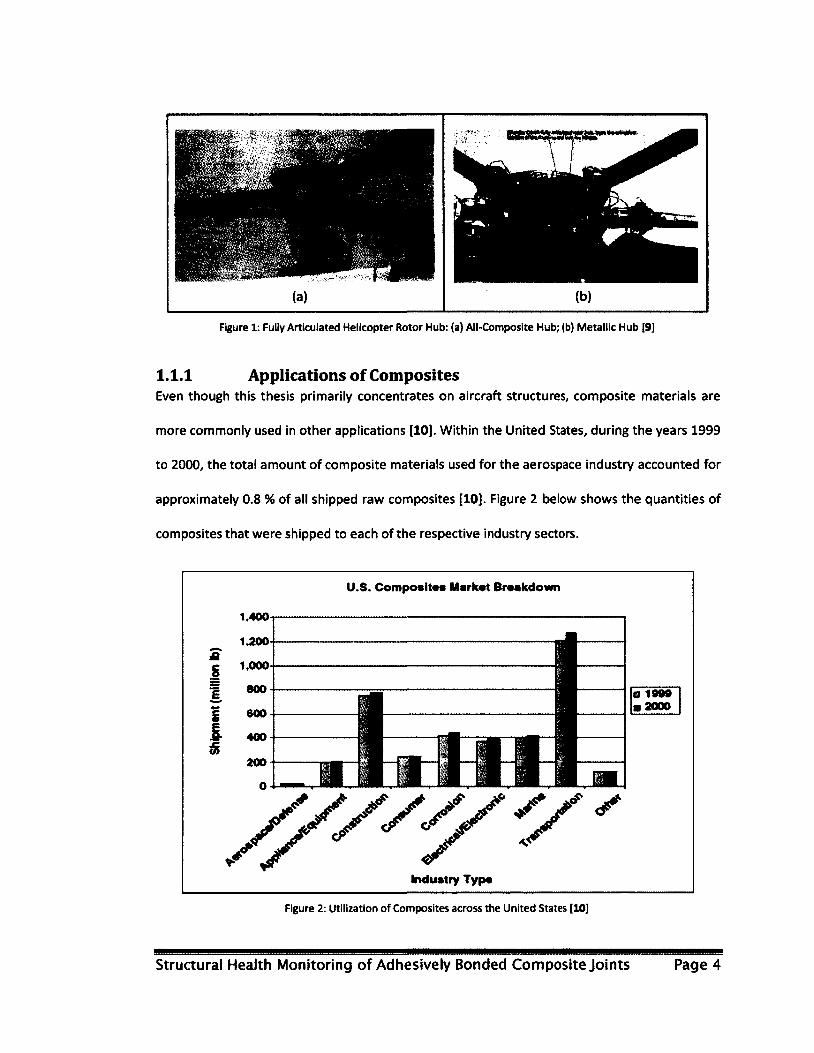
Figure 1: Fully Articulated Helicopter Rotor Hub: (a) All-Composite Hub; (b) Metallic Hub [9]
1.1.1 Applications of Composites Even though this thesis primarily concentrates on aircraft structures, composite materials are
more commonly used in other applications [10]. Within the United States, during the years 1999
to 2000, the total amount of composite materials used for the aerospace industry accounted for
approximately 0.8 % of all shipped raw composites [10]. Figure 2 below shows the quantities of
composites that were shipped to each of the respective industry sectors.
U.S. Composites Market Breakdown
1.400
s
ds
14(00
1,000
V/////// //s'y /
a 1999 • 2000
Industry Type
Figure 2: Utilization of Composites across the United States [10]
Struaural Health Monitoring of Adhesively Bonded Composite Joints Page 4

1.1.1.1 Aerospace Composite Application The United States Air Force was one of the first organizations to utilize composite materials in
the aerospace/defence industry. Composite materials on fighters such as the F-lll, F-14, F-15
and F-16 included such components as skins for the aerodynamic surfaces [10]. Introduction of
composites (primarily boron based fibres) for use on fighters enabled the reduction of weight of
the individual components by up to 35%. This reduction in weight allowed fighters to carry
heavier payload while increasing range [8,10,11]. After research into composites by the Air
Force during the Cold War, the civilian aircraft industry began to slowly implement composite
components as part of their structures [8]. Both Figure 3 and Figure 4 show composite
components on military (Northrop Grumman B-2 Bomber) and civilian (Airbus A320) aircraft; it
is clear that civilian aircraft utilize significantly less composite materials, a difference of
approximately 40% of the overall structural weight [11]. The difference of composite percentage
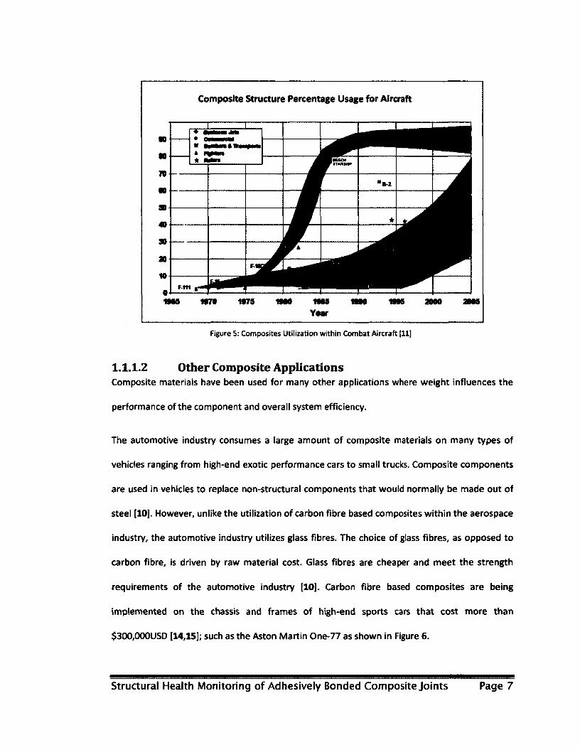
usage for both the A320 and the B-2 bomber are defined by their design requirements. Figure 5
shows a plot of composite usage percentage for many aircraft that have been produced with
various flight requirements over a 40 year time span beginning in 1965. It is clear from Figure 5
that since the 1960s composite usage has been on the rise for both the military and civilian
aerospace industries. Aircraft in the early 1970s utilized less than 5% according to the graph
while aircraft produced in the early 2000s utilized 30% (or less) of composites within their
structural weight. With the exception of the Beechcraft Starship and the Northrop Grumman B-2
bomber, all other aircraft structures are composed of no more than 30% composite; this was
true until recent introduction of the Boeing B787 [11,12]. The Beechcraft Starship was the first
of its kind to utilize significant amount of composite materials. However, due to the lack of
understanding of composite materials' performance and aging, the Starship was later removed
Struaural Health Monitoring of Adhesively Bonded Composite Joints Page 5
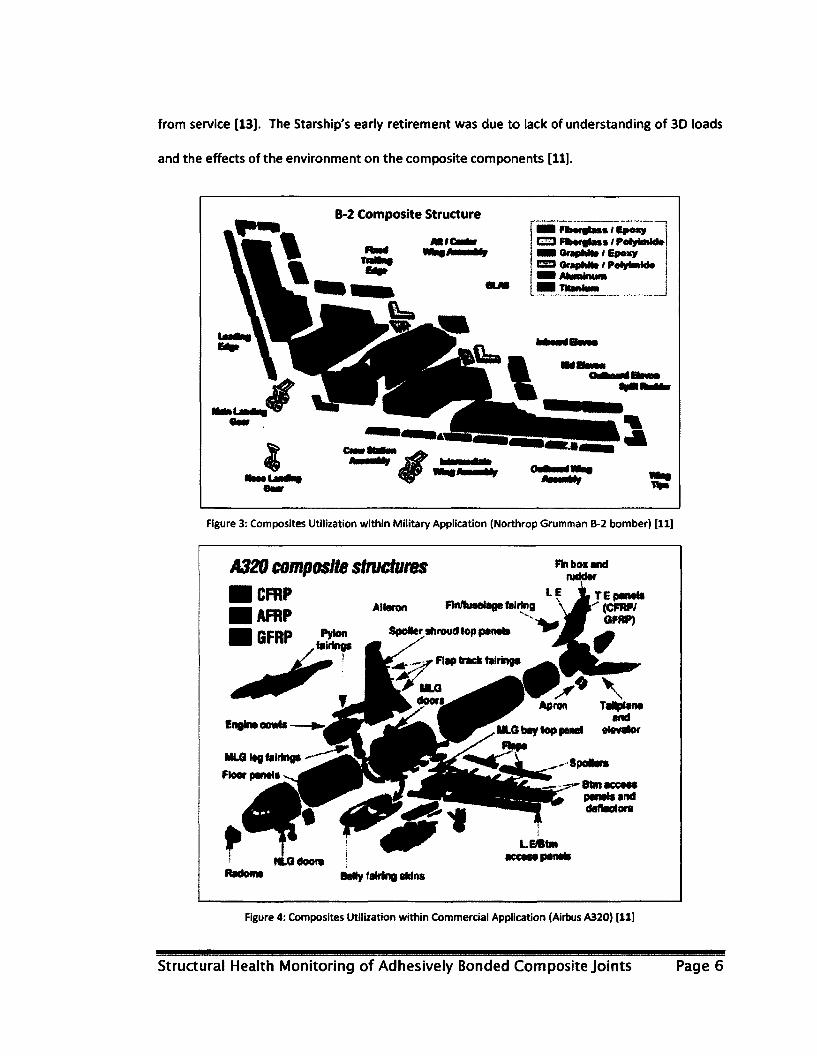
from service [13]. The Starship's early retirement was due to lack of understanding of 3D loads
and the effects of the environment on the composite components [11].
B-2 Composite Structure
Figure 3: Composites Utilization within Military Application (Northrop Grumman B-2 bomber) [11]
A320 composite structures
• CFRP • AFRP • GFRP
Alioron
Pylon , fairings
!
Fin box and rwklsr
LE jLTEpaiMlS Fin/fuselage lairing \ (CFRP/
GFRP) Spciierrfiroudtoppaneta ^
TaQplans and
MU3 bay top panel elsvslor
Flap track tairinga
MU2 lag fairing*
NLQdoora
Btmaccass panaia and dedadors
LBBton iccmpcflili
BaNy fairing sMns
Figure 4: Composites Utilization within Commercial Application (Airbus A320) [11]
Structural Health Monitoring of Adhesively Bonded Composite joints Page 6
Composite Structure Percentage Usage for Aircraft
1M5 1979 1978 1999 INS 1999 1M9 3000 2005
Figure 5: Composites Utilization within Combat Aircraft [11]
1.1.1.2 Other Composite Applications Composite materials have been used for many other applications where weight influences the
performance of the component and overall system efficiency.
The automotive industry consumes a large amount of composite materials on many types of
vehicles ranging from high-end exotic performance cars to small trucks. Composite components
are used in vehicles to replace non-structural components that would normally be made out of
steel [10]. However, unlike the utilization of carbon fibre based composites within the aerospace
industry, the automotive industry utilizes glass fibres. The choice of glass fibres, as opposed to
carbon fibre, is driven by raw material cost. Glass fibres are cheaper and meet the strength
requirements of the automotive industry [10]. Carbon fibre based composites are being
implemented on the chassis and frames of high-end sports cars that cost more than
$300,0001)SD [14,15]; such as the Aston Martin One-77 as shown in Figure 6.
Structural Health Monitoring of Adhesively Bonded Composite Joints Page 7
Figure 6: Automotive Composites: (a) Aston Martin One-77 [14]; (b) Aston Martin One-77 Cross-Section [15]
The sports industry also uses composites for sports products that require specific stiffness and
directional flexibility; these include but are not limited to golf sticks, hockey sticks, tennis
racquets and baseball bats. Through the selection of the proper fibres and fibre orientation,
manufacturers can acquire the correct stiffness that would be tailored for each player's swing.
The construction industry also uses composite materials for bridge repair; these would include
both glass fibre and carbon fibre doublers [10]. Also, within the construction industry, another
form of composite material that is widely used is reinforced concrete [16]. In concrete, the
reinforcing fibres are steel rods and the matrix is the concrete itself [16].
1.1.2 Basics of Composites Composite components are composed of two or more materials to create a single
entity/component. Of the two materials, one acts as the load carrying material while the other
acts as the load transfer medium. The load carrying material is a fibre while the load transfer
medium is a resin, as shown in Figure 7. Fibres can be of any material such as carbon, boron,
glass, graphite, steel, etc. The resin is some form of plastic, usually a thermoset; however, in
recent years, thermoplastics have been also used to make composite components.
Structural Health Monitoring of Adhesively Bonded Composite Joints Page 8
Resin Composite
Figure 7: Composite Composition [10]
A single ply (sheet) of composite material is formed by combining fibre and resin as shown in
Figure 7. Multiple plies are stacked onto each other to form a larger and thicker composite
component as shown in Figure 8(a). In addition to ply stacking, there exist other forms of
composite material that do not use continuous fibres, both of which are shown in Figure 8(b)
and Figure 8(c) [17]. Discontinuous fibres and partial fibres are chopped up from the same fibre
strand as that used for ply stacking [17]. Chopped fibres allow for distributed strength in all
directions and therefore allow the component to behave as an isotropic material. Because the
resin is allowed to cure while the component is near its final shape, complex curvature may be
obtained in a single step as compared to many required for alloys.
Continuous fibers Discontinuous fibers Particles
Figure 8: Composite Lay-up: (a) Continuous Fibres, (b) Discontinuous Fibres, and (c) Particle Fibres [17]
1.1.3 Joining of Composite Materials Joining of composite materials may be done using mechanical fastening or adhesive bonding
[18]. Both methods have their own advantages and disadvantages. In general, mechanical
fasteners' advantages include: no surface preparation, easy disassembly and easy inspection
Structural Health Monitoring of Adhesively Bonded Composite Joints Page 9

while disadvantages include: stress concentration and increased component count. Bonding
advantages include: smooth stress distribution and reduced component count while
disadvantages include: difficult disassembly (in some cases impossible), difficult inspection and
strict surface preparation requirements [8,18,19]. It may appear that bonded joint
disadvantages outnumber the advantages; however, when evaluated, both weight reduction
and smooth stress distribution overcome these disadvantages [20].
Adhesive bonding in the aerospace industry first appeared on the De Havilland Mosquito in the
1940s [21]. The Mosquito was built of plywood, balsa and spruce components. All of these
components were bonded using adhesives. During World War II, bombers were manufactured
using the aid of adhesives. However, aircraft during the war had an expected life of 600 hours
prior to being shot during combat. Full understanding of strength and limitations of adhesive
joints were not of concern as they were known to have a life greater than that of the bomber's
expected life. Aircraft which since have survived the war and have ever since been in storage,
have not shown any signs of major degradation as they have not been exposed to harsh weather
conditions as compared to current in-service aircraft.
Current in-service aircraft are exposed to harsh conditions and high loads. Non-composite
military in-service aircraft remain operational for more than 50 years while some non-composite
commercial aircraft such as B747 have spent more than 30 years in-service prior to retirement.
As these aircraft age in the presence of harsh environments and loads, components crack and
adhesive joints degrade which affect the safety and performance of the aircraft. To prolong the
life of components, composite patches may be bonded in areas of cracks to redistribute
stresses. Also, composite joints may be used on new aircraft to eliminate fasteners which create
stress concentrations that give rise for crack nucleation or composite delamination.
Structural Health Monitoring of Adhesively Bonded Composite Joints Page 10

1.1.3.1 Patch Bonded Repairs During the 1980s, many aging in-service mirage fighter aircraft of the Royal Australian Air Force
(RAAF) began to exhibit signs of cracking at the wing root skin as shown in Figure 9 [22]. Repair
of such damage could have been done through the use of aluminum doublers or composite
patches. Doublers would introduce a second layer of skin which would be riveted over the
cracked area. Rivets introduce additional locations where local stresses increase and therefore
increasing the probability of crack initiation. Composite patches may be used and bonded to the
wing surface to redistribute stresses without the addition of rivets. Composite patches were
chosen as opposed to aluminum doublers and were applied to the skin as shown in Figure 10.
The application of patches redistributed the local stress and therefore increased the life of the
component. The addition of patches to the cracked areas limited further crack growth; this is
demonstrated through the component life cycle graph found within Figure 11. The two curves
within the figure show an unpatched component and a patched component. Both components
were loaded using identical conditions and only the unpatched component exhibited crack
propagation. Similar repairs were carried out on cracked ribs of the Hercules aircraft within the
RAAF fleet.
Structural Health Monitoring of Adhesively Bonded Composite Joints Page 11
Crack nucleation
Areas
Figure 9: Australian Mirage III Crack Nucleation Locations [23]
X'/s'st
Boron
Figure 10: Australian Mirage III Patched Crack: (a) Repair Schematic and (b) Actual Repaired Wing Skin [23]
Structural Health Monitoring of Adhesively Bonded Composite Joints Page 12
Growth ttettcted
o «0 - Test terminated
1.0 No. o( programs
100
Figure 11: Influence of Patches on Crack Growth [23]
Consistency of all patch bonded repairs was achieved by following a well-accepted bonding
process. The Boeing Corporation process for surface preparation consisted of a phosphoric acid
gel-anodising procedure. There are two versions of this process; the first version is used on a
production line for which components can be dipped in a chemical bath. The second version of
this method was developed for in-field repair for which the component could not be submerged
in a chemical bath [21]. The second variation is called the Phosphoric Acid Non-Tank Anodizing
(PANTA) technique and was implemented on the mirage wing by the RAAF [22]. This process
ensures that the surface is contaminate-free and is ready for bonding.
The use of composite patches along with a proven bonding process has shown to be an
economical method for extending the life of aging aircraft. This method became the choice for
repair as patches were easy to fabricate and were corrosive resistant [24,25]. However, even
with the best fabrication and installation methods, patch bonded repairs must still be inspected
to ensure bond strength integrity. In some cases, bonds may appear to be safe; however the
bond may not have any load carrying capabilities. These types of bonds are known as kissing
Structural Health Monitoring of Adhesively Bonded Composite Joints Page 1B

bonds [26]. Kissing bonds are dangerous and unsafe for operation. Bonding of two components
together using a well-accepted method may result in a strong, weak or kissing bond. Kissing
bonds appear to have full adhesion between the surfaces; however, the bond fails well below
the design limit [26]. The failure may occur at 20% of the design load [21]. For that reason and
to avoid premature failure, it is important to investigate the integrtity of any bond, whether it
be between metal-to-metal, composite-to-metal or composite-to-composite.
Inspection of patches using advanced technology is necessary to ensure safety [27]. Inspection
of these patches may be done using the aid of advanced scanning techniques. Advanced
techniques include Non-Destructive Evaluations (NDE) and Structural Health Monitoring (SHM)
Systems [27,26]. NDE techniques may include technologies such as ultrasound inspections using
A-Scans, B-Scans, or C-scans (later described in section 2.1.1) [27]. SHM techniques include a
variety of new experimental technologies such as Acousto-Ultrasonic (AU) and Capacitance
Disbond Detection Technique (CDDT) [28,29].
All patches as well as their inspection technique must be certified so that an aircraft may
maintain airworthiness. Possible inspection techniques are discussed within the following
section.
1.2 Inspection of Structures
Safety is of utmost importance for all types of air transportation, especially for military and
civilian uses. Newly manufactured aircraft structures are scrutinized by quality control and
repaired structures are inspected within the field to prolong the life of the component.
Determination of how long a component is to properly function within in an aircraft can be
achieved in many ways, one such way is through the use of a Holistic Structural Integrity
Structural Health Monitoring of Adhesively Bonded Composite Joints Page 14
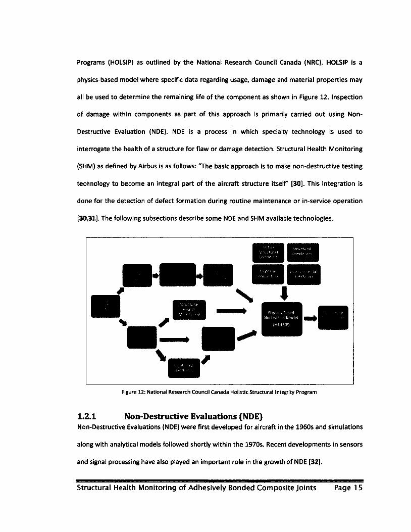
Programs (HOLSIP) as outlined by the National Research Council Canada (NRC). HOLSIP is a
physics-based model where specific data regarding usage, damage and material properties may
all be used to determine the remaining life of the component as shown in Figure 12. Inspection
of damage within components as part of this approach is primarily carried out using Non-
Destructive Evaluation (NDE). NDE is a process in which specialty technology is used to
interrogate the health of a structure for flaw or damage detection. Structural Health Monitoring
(SHM) as defined by Airbus is as follows: 'The basic approach is to make non-destructive testing
technology to become an integral part of the aircraft structure itself [30]. This integration is
done for the detection of defect formation during routine maintenance or in-service operation
[30,31]. The following subsections describe some NDE and SHM available technologies.
Figure 12: National Research Council Canada Holistic Structural Integrity Program
1.2.1 Non-Destructive Evaluations (NDE) Non-Destructive Evaluations (NDE) were first developed for aircraft in the 1960s and simulations
along with analytical models followed shortly within the 1970s. Recent developments in sensors
and signal processing have also played an important role in the growth of NDE [32].
Structural Health Monitoring of Adhesively Bonded Composite Joints Page 15

There are several NDE technologies that are used and trusted within the aerospace industry;
however, each has their advantages and disadvantages for the detection of different types of
defects. The seven NDE techniques used within industry are listed in order of popularity: visual
inspection, ultrasonic, eddy current, acoustic emission, X-Ray radiography, thermography and
shearography.
1.2.1.1 Visual Inspection Visual inspection is the most common form of NDE used today for in-service aircraft. This
technique involves having inspectors closely examine components using their eye sight for
surface or near surface defects. Due to the limitation of the human eye, technicians utilize
additional tools such as static optical microscopes or even scanning electron microscopes to
view damage. Visual inspection is limited by the viewing capabilities of the human eye.
Therefore, it may be difficult to identify the severity of damage, especially for micro-cracks. In
many cases where visual inspection reveals damage, components are removed from the aircraft
and sent out for further inspection utilizing sophisticated technologies.
In addition, new illumination chemicals (known as dye penetrants) have been utilized on cracked
surfaces to detect cracks under special lighting [32]. These chemicals are applied to the surface
of a structure and small amounts of the chemical seeps into cracks while the remainder of the
chemical is removed. Under special lighting, this chemical illuminates and reveals the crack.
This technique is very limited to optical viewing capabilities and is therefore very difficult to
implement on composite structures where damage occurs under the surface as delamination or
micro cracking within the matrix or fibres.
Structural Health Monitoring of Adhesively Bonded Composite Joints Page 16

1.2.1.2 Ultrasound Ultrasound (UT) inspection (also known as ultrasonic inspection) is an NDE technique in which
sound waves are guided through the structure for detection and evaluation of damage. Through
the analysis of UT signal attenuation, phase shift, reflection and scatter, damage can be found
and quantified. There are two forms of signal propagation methods that are used for UT: pulse-
echo and pitch-catch. Pulse-echo is a method in which a single transducer is used to send the UT
signal and the same transducer acts as a receiver which collects all the signals after they have
been reflected by edges and defects. Pitch-Catch is a method in which two transducers are used.
One transducer transmits signals while the other receives the signals. Both pulse-echo and
pitch-catch methodologies are used in different scan types to provide different image
resolutions.
There are three forms of ultrasound scan types: A, B and C scans; each one of these scans is
used for a specific application and provides different image resolution of damage. A-Scans are
the most basic form of UT inspections, they are used to scan as single point for damage; this is
done by scanning through the thickness of the component. Signals are sent from one free
surface and allowed to bounce back off another free surface so that it may be captured by the
transducer as shown in Figure 13. In the presence of damage, signals will reflect off the damage
and will be received by the transducer prior to receiving the backwall echo. Signal propagation
using pulse-echo of a component with a defect is shown in Figure 14.
Structural Health Monitoring of Adhesively Bonded Composite Joints Page 17
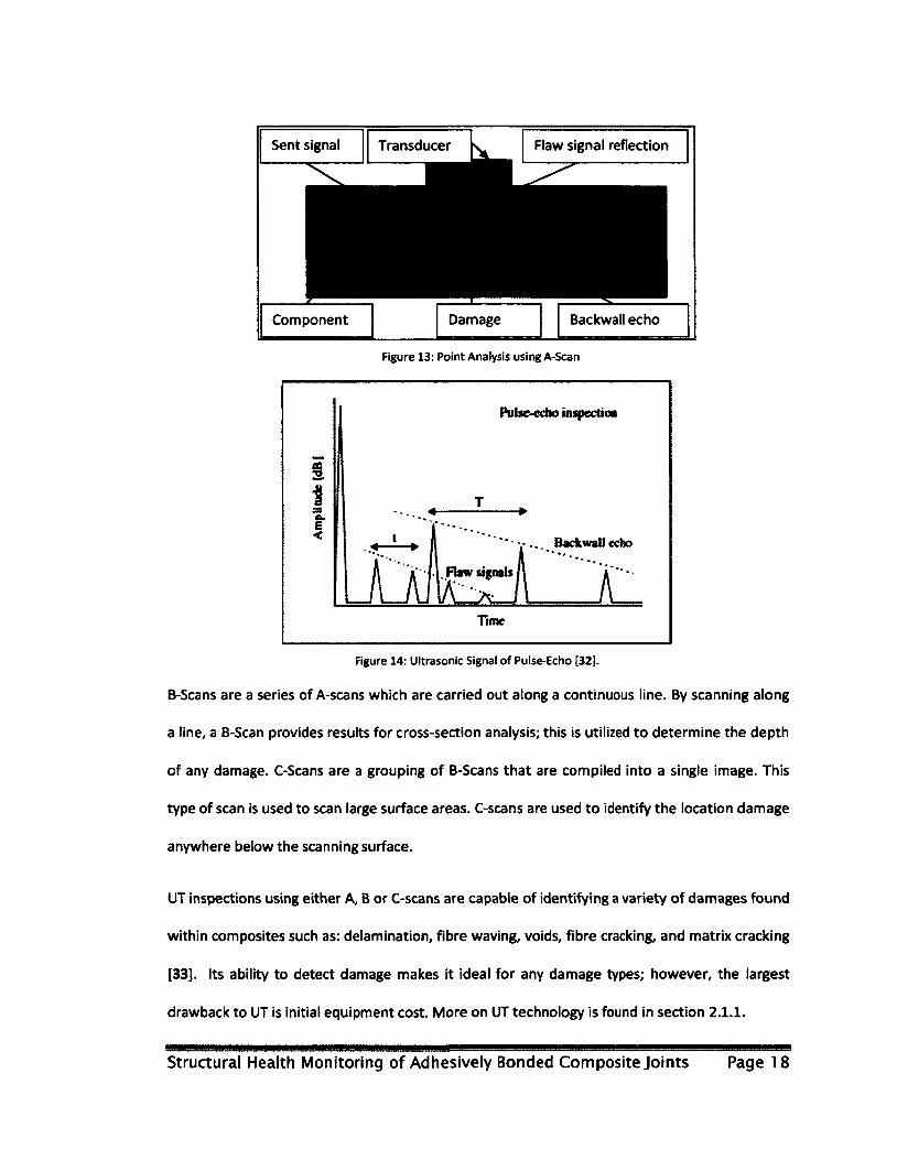
Sent signal Transducer k Flaw signal reflection
1MB Component Damage Backwall echo
Figure 13: Point Analysis using A-Scan
1 Pulse-echo inspection
I 1 T
4 e. E < , 1 » I * Y" Backwal,«cho
r'Aferii A" Time
Figure 14: Ultrasonic Signal of Pulse-Echo [32].
B-Scaris are a series of A-scans which are carried out along a continuous line. By scanning along
a line, a B-Scan provides results for cross-section analysis; this is utilized to determine the depth
of any damage. C-Scans are a grouping of B-Scans that are compiled into a single image. This
type of scan is used to scan large surface areas. C-scans are used to identify the location damage
anywhere below the scanning surface.
UT inspections using either A, B or C-scans are capable of identifying a variety of damages found
within composites such as: delamination, fibre waving, voids, fibre cracking, and matrix cracking
[33]. Its ability to detect damage makes it ideal for any damage types; however, the largest
drawback to UT is initial equipment cost. More on UT technology is found in section 2.1.1.
Structural Health Monitoring of Adhesively Bonded Composite Joints Page 18
1.2.1.3 Eddy Current Eddy current is an NDE technique in which a probe is used to measure the change in
electromagnetic impedance of a conductive structure. Change in the impedance is caused by a
change in strain within the structure which is usually caused by a defect [32].
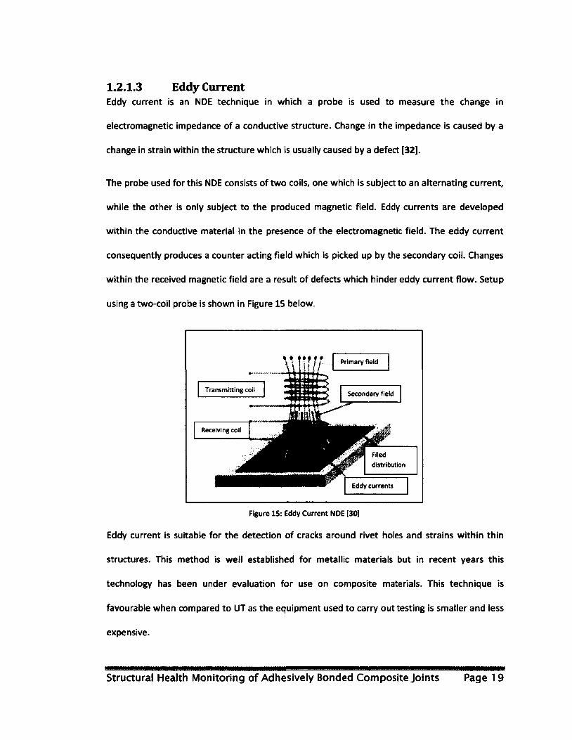
The probe used for this NDE consists of two coils, one which is subject to an alternating current,
while the other is only subject to the produced magnetic field. Eddy currents are developed
within the conductive material in the presence of the electromagnetic field. The eddy current
consequently produces a counter acting field which is picked up by the secondary coil. Changes
within the received magnetic field are a result of defects which hinder eddy current flow. Setup
using a two-coil probe is shown in Figure 15 below.
Primary field
Transmitting coil Secondary field
Receiving coil
Filed distribution
Eddy currents
Figure 15: Eddy Current NDE [30]
Eddy current is suitable for the detection of cracks around rivet holes and strains within thin
structures. This method is well established for metallic materials but in recent years this
technology has been under evaluation for use on composite materials. This technique is
favourable when compared to UT as the equipment used to carry out testing is smaller and less
expensive.
Structural Health Monitoring of Adhesively Bonded Composite Joints Page 19

1.2.1.4 Acoustic Emission Acoustic Emission (AE) is a passive NDE technique in which there are no transducers, just
sensors. Materials have stored elastic and plastic energy that are a result of applied loading.
Rapid release of stored energy results in acoustic waves which propagate through the structure.
Release of energy is a result of crack nucleation, crack propagation, fracture, fibre breakage,
matrix cracking or slippage of grains within the metallic structure. AE waves are registered by
sensors which are placed along the structure. Features such as signal duration, amplitude,
energy and travel time are used to determine different types of defects. Signals generated by
the structure have frequencies that can range anywhere from 10 KHz to 1 MHz [32].
Sensors used within the AE system are made of piezoelectric elements. These sensors are
bonded on the structure to form a large grid. Waves generated through rapid release of energy
register in many of the bonded sensors. Through triangulation using flight time of the signal,
algorithms are able to identify the location of the damage. However, signal processing is very
difficult as there is usually a lot or significant background noise.
1.2.1.5 X-Ray Radiography X-Ray Radiography is an NDE technique which utilizes X-Rays or Gamma rays to view defects
within the structure. Figure 16 shows an illustration of Radiography; this technology involves
the transmission of radiation onto the structure. A portion of the radiation is absorbed by the
structure in areas of defects. The unabsorbed portion of radiation which passes through the
structure is captured onto a photographic film. Defects within the structure which have
absorbed radiation appear on the film as areas with higher absorption [32].
Structural Health Monitoring of Adhesively Bonded Composite Joints Page 20
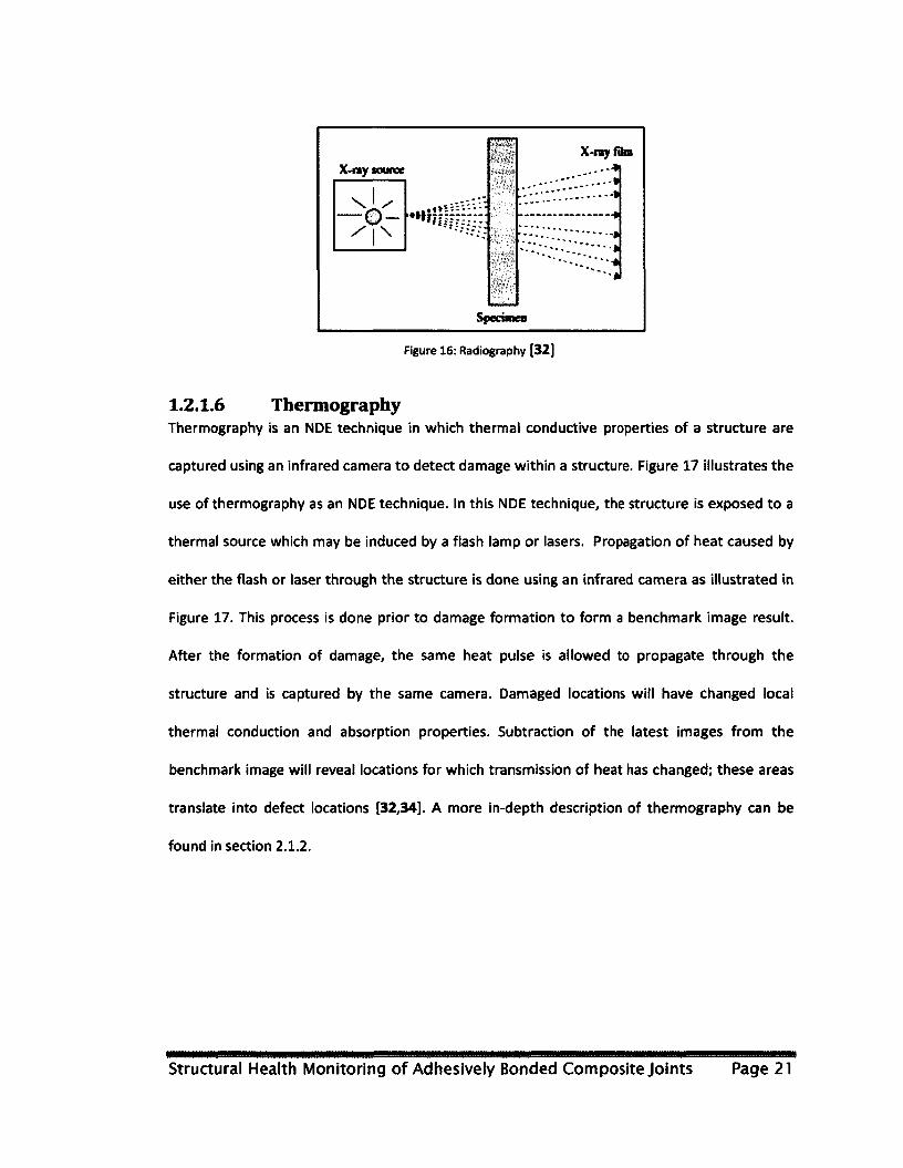
Specimen
X-ray film
—4
Figure 16: Radiography [32]
1.2.1.6 Thermography Thermography is an NDE technique in which thermal conductive properties of a structure are
captured using an infrared camera to detect damage within a structure. Figure 17 illustrates the
use of thermography as an NDE technique. In this NDE technique, the structure is exposed to a
thermal source which may be induced by a flash lamp or lasers. Propagation of heat caused by
either the flash or laser through the structure is done using an infrared camera as illustrated in
Figure 17. This process is done prior to damage formation to form a benchmark image result.
After the formation of damage, the same heat pulse is allowed to propagate through the
structure and is captured by the same camera. Damaged locations will have changed local
thermal conduction and absorption properties. Subtraction of the latest images from the
benchmark image will reveal locations for which transmission of heat has changed; these areas
translate into defect locations [32,34]. A more in-depth description of thermography can be
found in section 2.1.2.
Structural Health Monitoring of Adhesively Bonded Composite Joints Page 21

Load
Specimen
Figure 17: Thermography [32]
1.2.2 Structural Health Monitoring (SHM) Health Monitoring (HM) is the analysis of a systems performance, throughout its life cycle; it is
applicable to aerospace structures, engines, civil structures and many other systems. Each
application of HM is done in a different manner and for a different purpose. For example, HM on
engines is done to collect and analyze specific parameters on the performance of an engine to
maintain highest running efficiency and to extend the life of an engine. While HM on structures
are done to detected damage formation prior to component failure so that repair is cost
effective and safety is not compromised. When HM is applied to aerospace or civil structures, it
is known as Structural Health Monitoring (SHM).
SHM is very similar to NDE as it is used in the detection of damage for new and in-service
aircraft. SHM integration within a structure is very similar to a human nervous system [30], as
shown Figure 18. The system consists of two parts: the interrogator and the sensor network.
The interrogator acts in similar manner as the brain while the sensor network acts as the nerves
within the human tissue. While SHM systems may vary in design, complexity and purpose, they
always have both an interrogator and a sensor network.
Structural Health Monitoring of Adhesively Bonded Composite Joints Page 22

Figure 18: Aircraft Nervous System [30,31]
There are two basic approaches to SHM design; the first is focused on the reduction of
maintenance cost while the second is focused around the design of new aircraft. Reduction of
maintenance cost can be achieved by carrying out maintenance when indicated by the onboard
SHM system. However, this will not be achieved until SHM systems are found to be reliable.
Establishing system reliability will be achieved by first implementing SHM systems as data
collectors. During routine maintenance, SHM monitored areas will be inspected and damage
evaluated. Once these SHM systems have been found to be effective, maintenance will be
carried out once indicated necessary by the SHM systems. The reduction in maintenance has a
potential cost savings of up to 75% [35]. In addition to the implementation of SHM systems for
maintenance based analysis on older aircraft, SHM will be used to aid in the design of next
generation aircraft. New aircraft will be under-designed to be lighter and more fuel efficient as
there will be less need for redundancy of aircraft structure [35]. However, prior to integration
on new or old aircraft, the SHM systems must be tested in the laboratory to evaluate their
effectiveness and reliability for the detection of damage initiation and growth.
There are two major types of SHM systems available on the market: health monitoring and load
monitoring [30]. Health Monitoring Systems (HMS) are those that directly seek defects within a
structure, while Load Monitoring Systems (LMS) monitor flight parameters which in turn are
Structural Health Monitoring of Adhesively Bonded Composite Joints Page 23
used to predict probability of defects [30]. LMS are used to monitor loads and strains using Fibre
Bragg Gratings (FBG) or strain gauges. HMS are used to detect structural damage through the
use of: Eddy current, Capacitance Disbond Detection Technique (CDDT), Comparative Vacuum
Monitoring (CVM), Surface Mountable Crack Detection System (SMCDS) and Acousto-Ultrasonic
(AU). The following sub-sections describe each of the passive and active systems and their basic
physics.
1.2.2.1 Fibre Bragg Gratings (FBG) Stresses produced during loading of a structure may be found by knowing both the modulus of
the material and the strain of the materials. Fibre Bragg Grating (FBG) is one technology that
may be used to measure strains.
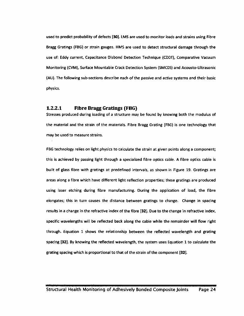
FBG technology relies on light physics to calculate the strain at given points along a component;
this is achieved by passing light through a specialized fibre optics cable. A fibre optics cable is
built of glass fibre with gratings at predefined intervals, as shown in Figure 19. Gratings are
areas along a fibre which have different light reflection properties; these gratings are produced
using laser etching during fibre manufacturing. During the application of load, the fibre
elongates; this in turn causes the distance between gratings to change. Change in spacing
results in a change in the refractive index of the fibre [32]. Due to the change in refractive index,
specific wavelengths will be reflected back along the cable while the remainder will flow right
through. Equation 1 shows the relationship between the reflected wavelength and grating
spacing [32]. By knowing the reflected wavelength, the system uses Equation 1 to calculate the
grating spacing which is proportional to that of the strain of the component [32].
Structural Health Monitoring of Adhesively Bonded Composite Joints Page 24
Incident light
Gratings
Reflected light
Distance between gratings
Figure 19: Fibre Bragg Gratings [36]
= 2nA Equation 1
Where:
• Awis reflected wave length, • /X is the spacing between gratings and • n is the average refractive index.
FBG contain a large number of gratings along a single fibre; for that reason they may be used to
measure strain in many different locations along a single fibre using the same acquisition system
and in/out port.
FBG have been tested in the past on military aircraft such as the F-22 and significant research
has been carried out on both metallic and composite components. One of the largest drawbacks
to FBGs is integration with the structure. There are two integration methods, internal to the
structure or external to the structure. Internal integration within composite materials allows the
FBG to be embedded along with many fibres within the laminate. However, FBG fibres are
significantly larger than common carbon and boron fibres which make the area around them
susceptible to failure within the matrix.
Structural Health Monitoring of Adhesively Bonded Composite Joints Page 25
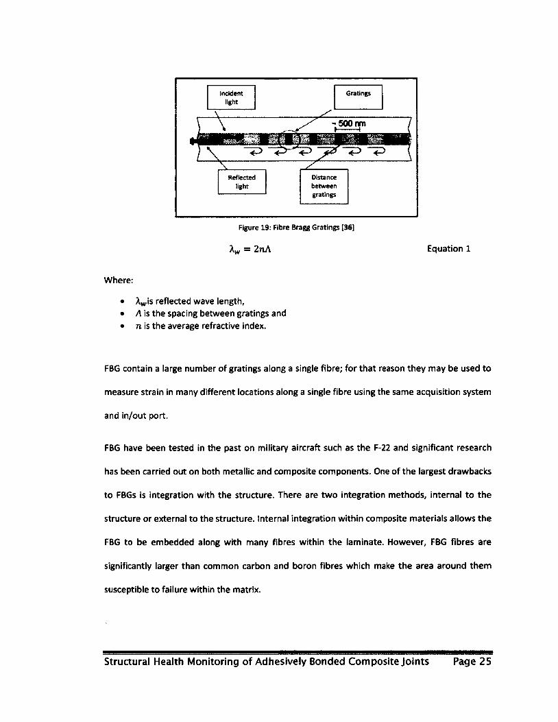
1.2.2.2 Strain Gauges (SG) Strain gauges (SG) are another type of sensors used to monitor loads on a structure and are very
similar to FBG. Unlike FBG, SG relies on electrical physics to calculate the strain at a particular
location on the component. Strain measurements of the component are obtained by passing
current though the sensor and measuring its resistance, which is a function of the strain
experienced by the SG. A simple SG, such as the one shown in Figure 20(a), is composed of a
series of wire windings. When elongated or compressed, the windings experience a change in
cross-sectional area of the wire. The change in area limits or promotes the passing of electrons
(i.e. changing the resistance of the sensor) [37,38]. The change in resistance can be calculated by
placing the SG into a quarter-bridge strain gauge circuit as illustrated in Figure 20(b) [37,38]. By
knowing the resistance, one can calculate the strain within the area of the gauge.
Tension causes resistance increase
Resistance measured between these points
Gauge insensitive to lateral forces
Compression causes resistance decrease
Figure 20: Strain Gauge and Circuit: (a) Typical Strain Gauge; (b) Typical Quarter Bridge Circuit [37]
Both the FBG and SG sensors output the same type of information (i.e. strain). Damage
identification using either FBG or SG is done by comparing the output strains to a
predetermined aircraft load strain model. Areas which output significantly higher or lower
strains, as compared to the model, indicate the presence of damage [32].
1.2.2.3 Eddy Current Eddy Current technology for SHM utilizes the same principles as those for the NDE technique
described in section 1.2.1.3 [30]. However, unlike NDE sensors which are handheld, SHM
Structural Health Monitoring of Adhesively Bonded Composite Joints Page 26
sensors are more compact and are surface mountable, see Figure 21. Eddy current sensors are
predominantly used for detecting defects within metallic structures; however, it has been
shown that they can also be used on conductive composite materials [29].
Eddy current sensor
Component
Figure 21: Typical Eddy Current Sensor [30]
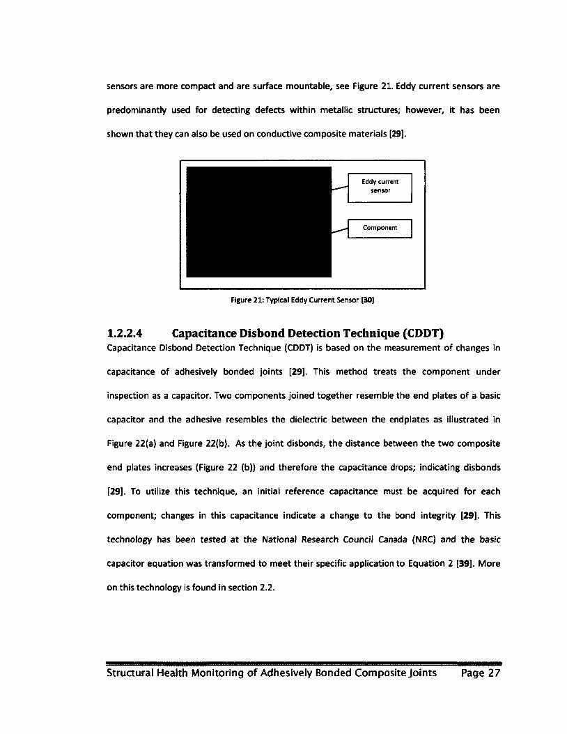
1.2.2.4 Capacitance Disbond Detection Technique (CDDT) Capacitance Disbond Detection Technique (CDDT) is based on the measurement of changes in
capacitance of adhesively bonded joints [29]. This method treats the component under
inspection as a capacitor. Two components joined together resemble the end plates of a basic
capacitor and the adhesive resembles the dielectric between the endplates as illustrated in
Figure 22(a) and Figure 22(b). As the joint disbonds, the distance between the two composite
end plates increases (Figure 22 (b)) and therefore the capacitance drops; indicating disbonds
[29]. To utilize this technique, an initial reference capacitance must be acquired for each
component; changes in this capacitance indicate a change to the bond integrity [29]. This
technology has been tested at the National Research Council Canada (NRC) and the basic
capacitor equation was transformed to meet their specific application to Equation 2 [39]. More
on this technology is found in section 2.2.
Structural Health Monitoring of Adhesively Bonded Composite Joints Page 27
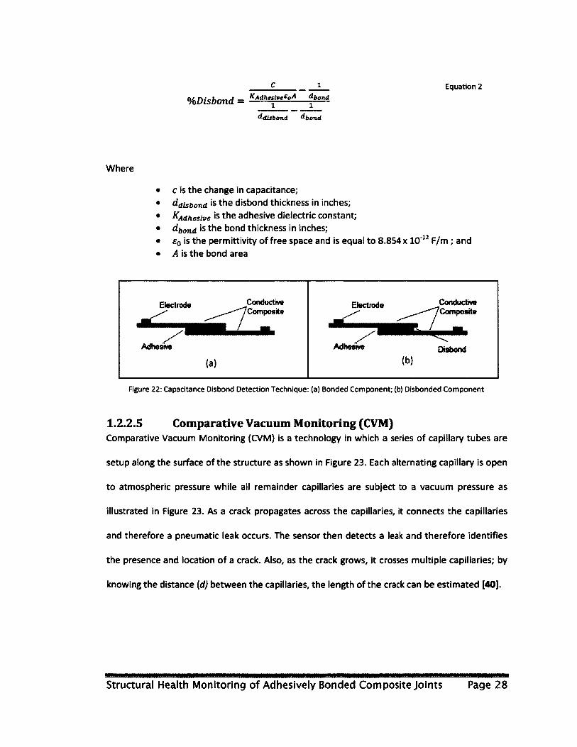
C 1
%Disbond = K*dh"™£°A ^
ddisbond ^bond
Equation 2
Where
• c is the change in capacitance; • daisbona is the disbond thickness in inches; • KAdhesive's the adhesive dielectric constant; • dbond is the bond thickness in inches; • £q is the permittivity of free space and is equal to 8.854 x 10"12 F/m; and • A is the bond area
Electrode Conductive Electrode Conductive Electrode —7Composite
Electrode "^Composite
Adhesive^ Adhesive^' Disbond
(a) (b)
Figure 22: Capacitance Disbond Detection Technique: (a) Bonded Component; (b) Disbonded Component
1.2.2.5 Comparative Vacuum Monitoring (CVM) Comparative Vacuum Monitoring (CVM) is a technology in which a series of capillary tubes are
setup along the surface of the structure as shown in Figure 23. Each alternating capillary is open
to atmospheric pressure while all remainder capillaries are subject to a vacuum pressure as
illustrated in Figure 23. As a crack propagates across the capillaries, it connects the capillaries
and therefore a pneumatic leak occurs. The sensor then detects a leak and therefore identifies
the presence and location of a crack. Also, as the crack grows, it crosses multiple capillaries; by
knowing the distance (d) between the capillaries, the length of the crack can be estimated [40].
Structural Health Monitoring of Adhesively Bonded Composite Joints Page 28

CVM sensors can only be mounted on the surface of a structure and therefore can only detect
surface defects, primarily cracks. This technology also requires continuous vacuum pressure so
an air compressor must be running continually while interrogating the structure.
Open Pressurized capttaries capillaries d
Figure 23: CVM Sensor [30]
1.2.2.6 Surface Mountable Crack Detection System (SMCDS) Surface Mountable Crack Sensors (SMCS) are very similar to that of CVM sensors. However,
SMCS are composed of a conductive paint rather than capillary tubes as illustrated in Figure 24.
When the component is being interrogated, low current with will pass through the wire. When
cracks grow through the SMCS, they break the paint. The conductive path changes to an open
circuit and the system identifies the presence of a crack. The location of the crack is determined
by the location of the broken conductive paths. Similar to CVM, the size of the crack can be
determined by knowing how many paint strips the crack has gone through [41]. More
information on SMCS is found in section 2.2.2.
SMCS sensor
Figure 24: SMCS Sensor
Structural Health Monitoring of Adhesively Bonded Composite Joints Page 29
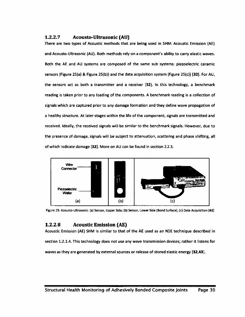
1.2.2.7 Acousto-Ultrasonic (AU) There are two types of Acoustic methods that are being used in SHM: Acoustic Emission (AE)
and Acousto-Ultrasonic (AU). Both methods rely on a component's ability to carry elastic waves.
Both the AE and AU systems are composed of the same sub systems: piezoelectric ceramic
sensors (Figure 25(a) & Figure 25(b)) and the data acquisition system (Figure 25(c)) [32]. For AU,
the sensors act as both a transmitter and a receiver [32]. In this technology, a benchmark
reading is taken prior to any loading of the components. A benchmark reading is a collection of
signals which are captured prior to any damage formation and they define wave propagation of
a healthy structure. At later stages within the life of the component, signals are transmitted and
received. Ideally, the received signals will be similar to the benchmark signals. However, due to
the presence of damage, signals will be subject to attenuation, scattering and phase shifting, all
of which indicate damage [32]. More on AU can be found in section 2.2.3.
Wire Connector
Piezoelectric Wafer
(a)
Figure 25: Acousto-Ultrasonic: (a) Sensor, Upper Side; (b) Sensor, Lower Side (Bond Surface); (c) Data Acquisition [42]
1.2.2.8 Acoustic Emission (AE) Acoustic Emission (AE) SHM is similar to that of the AE used as an NDE technique described in
section 1.2.1.4. This technology does not use any wave transmission devices; rather it listens for
waves as they are generated by external sources or release of stored elastic energy [32,43].
Structural Health Monitoring of Adhesively Bonded Composite Joints Page 30

1.3 Inspection of Patch Repairs
The introduction of patch bonded repairs especially by the Royal Australian Air Force (RAAF) has
led to an increase in research for analysis techniques required for certifying these repairs. The
certification process has led to numerical model developments as well as NDE and SHM system
evaluations for early detection of patch failure.
Numerical models for the evaluation of patch strength as well as crack growth of the repaired
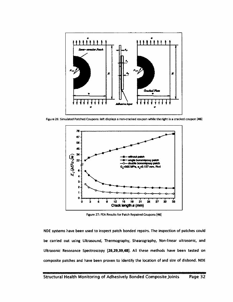
metallic surface have been studied in the past [44,45,46]. Finite Element Analysis (FEA) has been
employed to analyze the effects of a patch on crack repaired aluminum alloys by Quinas [46],
Figure 26 shows an example of two models that were developed within FEA software to see the
effects of a patch on the stress intensity factor (K)) by Quinas. These two models were tested
and evaluated, results of which are presented in Figure 27. It is clear from Figure 27, that the use
of a patch reduces the crack's stress intensity factor and therefore extends the life of the
component. In addition to FEA, analytical equation development was also performed by Chorng-
Fuh Liu and many others [47]. Equations were developed for the evaluation of the stress
intensity factor; which was later used to predict the remaining life of the component. In 2007,
Fujimoto looked at FEA for crack growth and life analysis for different crack and disbond fronts
[44]. However, even with the best prediction software, it is necessary to inspect the patch
repairs during service of the aircraft.
Structural Health Monitoring of Adhesively Bonded Composite Joints Page 31
liililLL Sum— imiarJPauk
TTTTTTTT
t t t l t t t t
\
K
AdSmiv*. taper
OadWJfan
TTrnrnr
Figure 26: Simulated Patched Coupons: left displays a non-cracked coupon while the right is a cracked coupon [46]
87-
46-
34-
• ungteborettfepoxypvich
G ««65 MP«, •-0.177 am. FU4
9 12 16 18 21 24 27 30 33 0 3 8 Crack length a (mm)
Figure 27: FEA Results for Patch Repaired Coupons [46]
NDE systems have been used to inspect patch bonded repairs. The inspection of patches could
be carried out using Ultrasound, Thermography, Shearography, Non-linear ultrasonic, and
Ultrasonic Resonance Spectroscopy [26,29,39,48]. All these methods have been tested on
composite patches and have been proven to identify the location of and size of disbond. NDE
Structural Health Monitoring of Adhesively Bonded Composite Joints Page 32
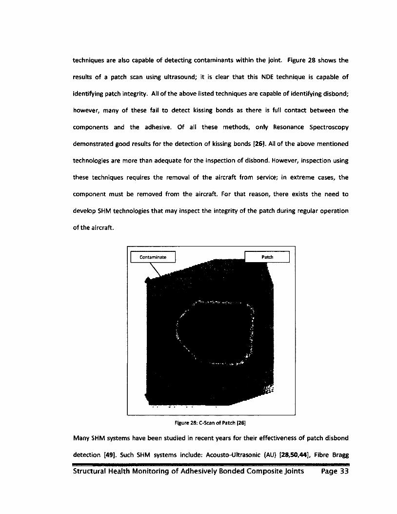
techniques are also capable of detecting contaminants within the joint. Figure 28 shows the
results of a patch scan using ultrasound; it is clear that this NDE technique is capable of
identifying patch integrity. All of the above listed techniques are capable of identifying disbond;
however, many of these fail to detect kissing bonds as there is full contact between the
components and the adhesive. Of all these methods, only Resonance Spectroscopy
demonstrated good results for the detection of kissing bonds [26]. Ail of the above mentioned
technologies are more than adequate for the inspection of disbond. However, inspection using
these techniques requires the removal of the aircraft from service; in extreme cases, the
component must be removed from the aircraft. For that reason, there exists the need to
develop SHM technologies that may inspect the integrity of the patch during regular operation
of the aircraft.
Patch Contaminate
Figure 28: C-Scan of Patch [26]
Many SHM systems have been studied in recent years for their effectiveness of patch disbond
detection [49], Such SHM systems include: Acousto-Ultrasonic (AU) [28,50,44], Fibre Bragg
Structural Health Monitoring of Adhesively Bonded Composite Joints Page 33

Gratings (FBG) [25], Strain Gauges (SG) [27,51] and Surface Mountable Crack Detection System
(SMCDS) [52]. All of these systems were tested on composite-to-metallic coupons and in many
cases an attempt was made to monitor crack and disbond propagation. SG technology is one of
the most basic forms of SHM technology used for monitoring patch disbond. Analysis of SG-
produced data is easy and effective, provided that loads and strains on the component are well
understood. SMCDS is also a very basic system which can be implemented to monitor crack
formation within the adhesive along the edges of any patch. Amongst all described SHM
technologies, AU has demonstrated much potential for the detection of different patch failure
modes. However, this technology is susceptible to many external influences such as noise; thus
making it difficult to analyze the data. There is much research that has been done using AU
systems and their underlying Lamb wave physics (later described in section 2.2.3). Extensive
research has shown the effectiveness of AU systems on isotropic mediums. However, there is
ongoing research to test the effectiveness of this technology on composite structures.
All these NDE and SHM technologies have been tested and evaluated in past research. However,
much of this research has been carried out on composite-to-metallic joints; none of the
techniques have been evaluated on composite-to-composite joints. This thesis is focused on the
evaluation of new SHM systems for their ability to identify and quantify disbond on composite-
to-composite joints.
1.4 Conclusion
Composite materials have been replacing traditional metallic materials since the 1970s. The
amount of composites used in any particular industry is highly depended on their advantages
and disadvantages for their specific application. While some industries have continued to
increase the use of composites at high rates, the aerospace industry has progressed at a slower
Structural Health Monitoring of Adhesively Bonded Composite Joints Page 34

rate. The aerospace industry cannot tolerate failure and therefore a method of identifying the
component's reaming life is of utmost necessity. NDE techniques have been used in the past to
evaluate structural health; however, this process is time consuming and costly. The introduction
of SHM technologies on aircraft may reduce inspection times as well as cost.
Structural Health Monitoring of Adhesively Bonded Composite Joints Page 35

Chapter 2.0: Selection of Damage Detection Systems
The focus of this thesis was to determine the effectiveness of multiple off-the-shelf Structural
Health Monitoring (SHM) Systems for the detection of disbond of a composite-to-composite
joint. There were many SHM systems mentioned within Chapter 1; however, only a limited
number of them were used within this research study. The selected SHM systems were those
which had the potential for the detection of defects in both composite and metallic structures.
SHM systems were evaluated on metallic structures prior to composites, as metallic structures
provide a less complex analysis scenario.
In addition to SHM systems, a number of Non-Destructive Evaluations (NDE) techniques were
used to validate the performance of the SHM systems used within this study.
This chapter discusses all the SHM systems and NDE techniques used within this study as well as
reason(s) for their selection.
2.1 Non-Destructive Evaluation (NDE) Systems
Inspection of coupons in this study was done using ultrasound as well as pulse thermography.
Pulse thermography is not a certified NDE technique. However, thermography has been used in
the past and has been shown to provide acceptable inspection results as those which were
obtained using ultrasound for patch bonded repairs [29]. The following subsections describe
both ultrasound and thermography inspections.
2.1.1 Ultrasound Inspection
Ultrasound inspection (UT) is one of the most utilized NDE techniques within the aerospace
industry. UT, as mentioned in section 1.2.1.2, uses high frequency sound waves to interrogate
Structural Health Monitoring of Adhesively Bonded Composite Joints Page 36
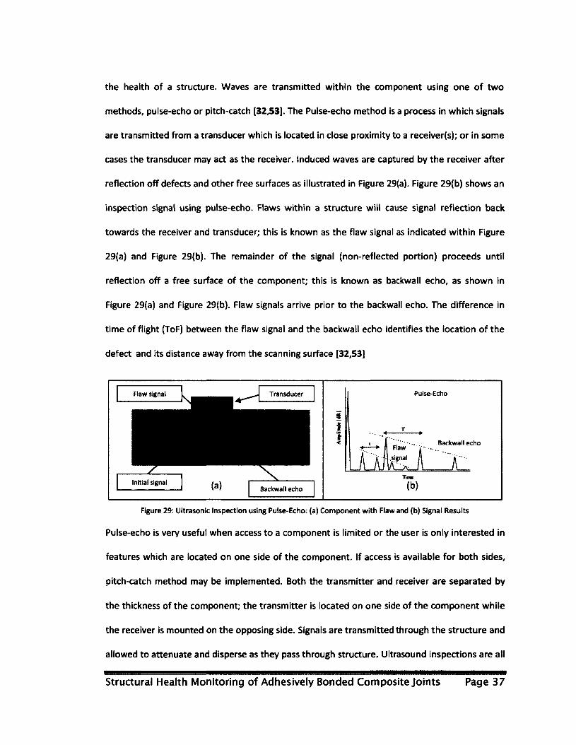
the health of a structure. Waves are transmitted within the component using one of two
methods, pulse-echo or pitch-catch [32,53]. The Pulse-echo method is a process in which signals
are transmitted from a transducer which is located in close proximity to a receiver(s); or in some
cases the transducer may act as the receiver. Induced waves are captured by the receiver after
reflection off defects and other free surfaces as illustrated in Figure 29(a). Figure 29(b) shows an
inspection signal using pulse-echo. Flaws within a structure will cause signal reflection back
towards the receiver and transducer; this is known as the flaw signal as indicated within Figure
29(a) and Figure 29(b). The remainder of the signal (non-reflected portion) proceeds until
reflection off a free surface of the component; this is known as backwall echo, as shown in
Figure 29(a) and Figure 29(b). Flaw signals arrive prior to the backwall echo. The difference in
time of flight (ToF) between the flaw signal and the backwall echo identifies the location of the
defect and its distance away from the scanning surface [32,53]
Pulse-Echo Transducer
Backwall echo
Backwall echo
Figure 29: Ultrasonic Inspection using Pulse-Echo: (a) Component with Flaw and (b) Signal Results
Pulse-echo is very useful when access to a component is limited or the user is only interested in
features which are located on one side of the component. If access is available for both sides,
pitch-catch method may be implemented. Both the transmitter and receiver are separated by
the thickness of the component; the transmitter is located on one side of the component while
the receiver is mounted on the opposing side. Signals are transmitted through the structure and
allowed to attenuate and disperse as they pass through structure. Ultrasound inspections are all
Structural Health Monitoring of Adhesively Bonded Composite Joints Page 37
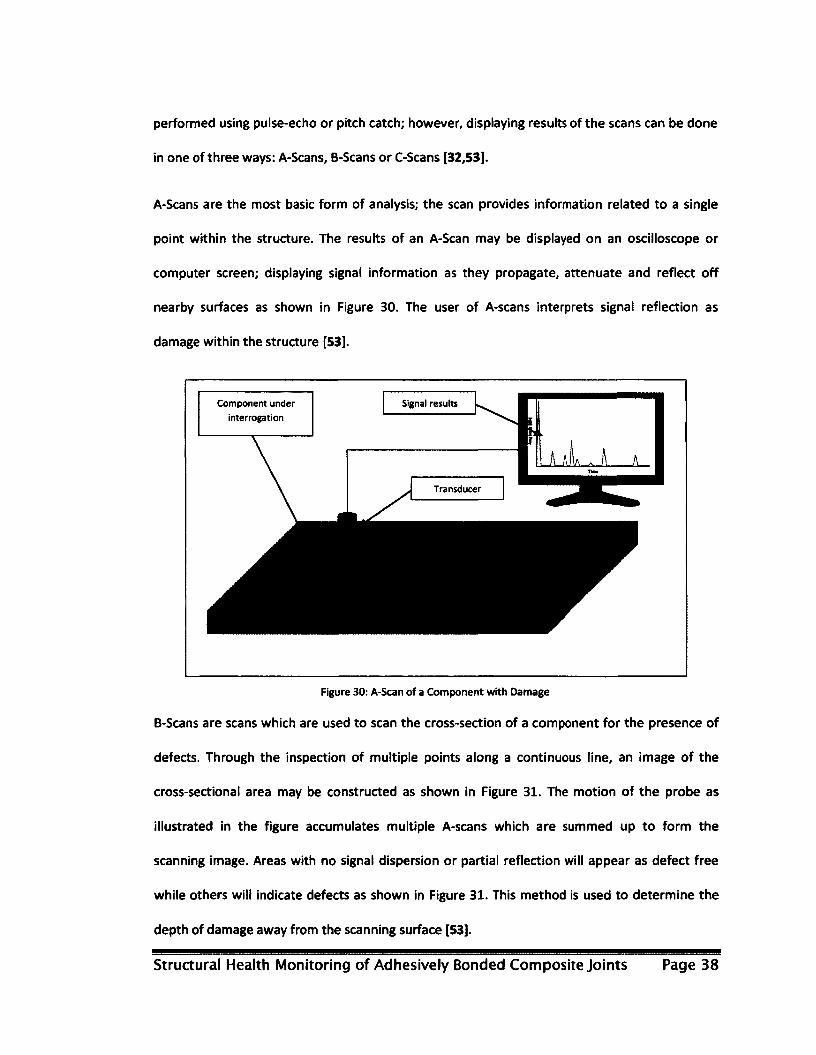
performed using pulse-echo or pitch catch; however, displaying results of the scans can be done
in one of three ways: A-Scans, B-Scans or C-Scans [32,53].
A-Scans are the most basic form of analysis; the scan provides information related to a single
point within the structure. The results of an A-Scan may be displayed on an oscilloscope or
computer screen; displaying signal information as they propagate, attenuate and reflect off
nearby surfaces as shown in Figure 30. The user of A-scans interprets signal reflection as
damage within the structure [53].
Component under
interrogation
Signal results
Transducer
Figure 30: A-Scan of a Component with Damage
B-Scans are scans which are used to scan the cross-section of a component for the presence of
defects. Through the inspection of multiple points along a continuous line, an image of the
cross-sectional area may be constructed as shown in Figure 31. The motion of the probe as
illustrated in the figure accumulates multiple A-scans which are summed up to form the
scanning image. Areas with no signal dispersion or partial reflection will appear as defect free
while others will indicate defects as shown in Figure 31. This method is used to determine the
depth of damage away from the scanning surface [53].
Structural Health Monitoring of Adhesively Bonded Composite Joints Page 38
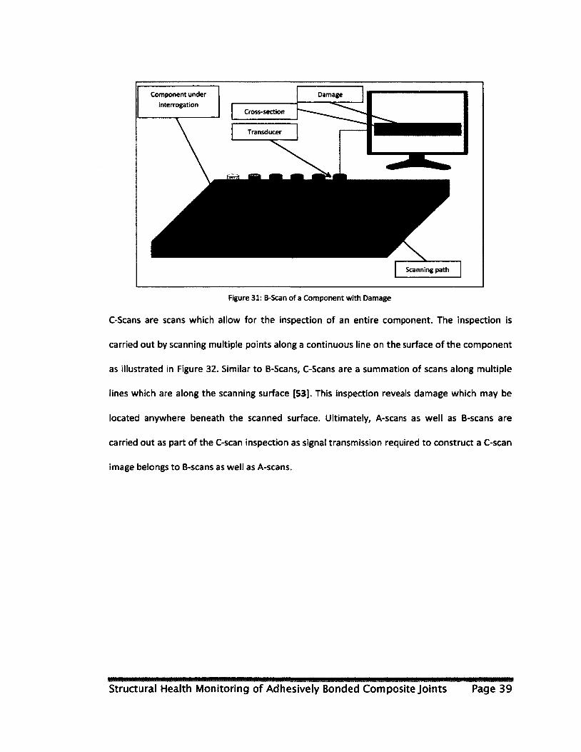
Component under
interrogation
Damage
Transducer
Scanning path
Figure 31: B-Scan of a Component with Damage
C-Scans are scans which allow for the inspection of an entire component. The inspection is
carried out by scanning multiple points along a continuous line on the surface of the component
as illustrated in Figure 32. Similar to B-Scans, C-Scans are a summation of scans along multiple
lines which are along the scanning surface [53]. This inspection reveals damage which may be
located anywhere beneath the scanned surface. Ultimately, A-scans as well as B-scans are
carried out as part of the C-scan inspection as signal transmission required to construct a C-scan
image belongs to B-scans as well as A-scans.
Structural Health Monitoring of Adhesively Bonded Composite Joints Page 39
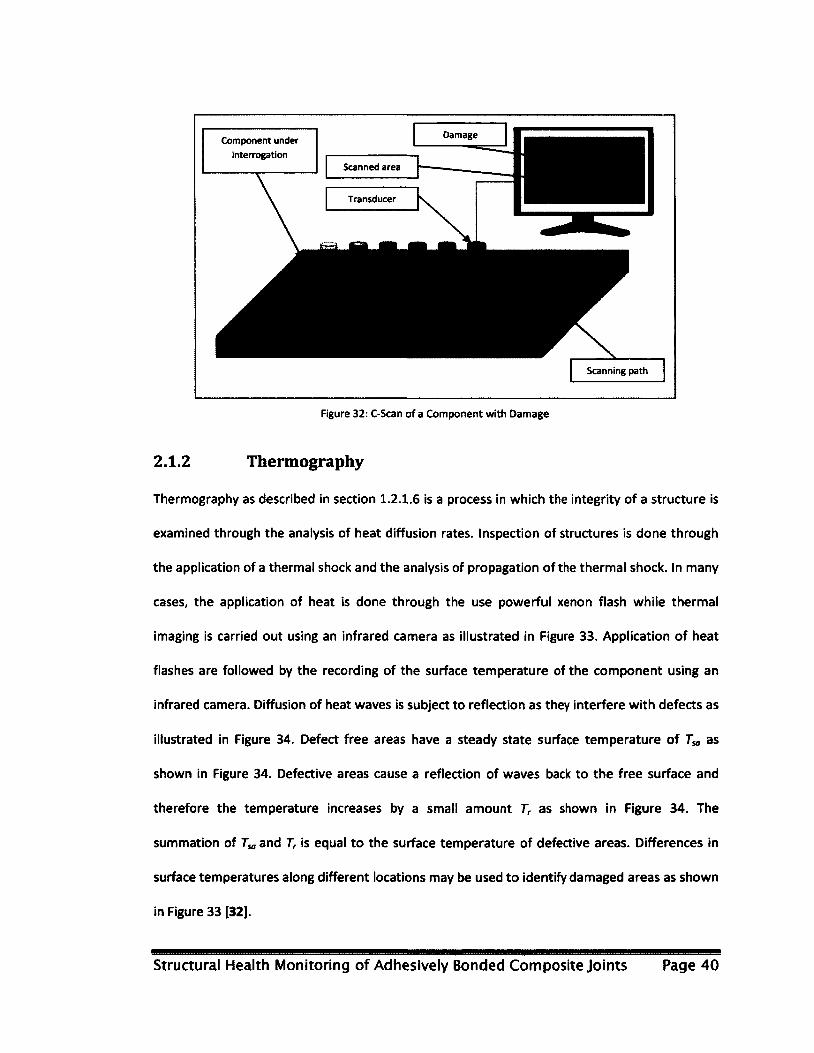
Damage Component under
interrogation
Transducer
Scanning path
Figure 32: C-Scan of a Component with Damage
2.1.2 Thermography
Thermography as described in section 1.2.1.6 is a process in which the integrity of a structure is
examined through the analysis of heat diffusion rates. Inspection of structures is done through
the application of a thermal shock and the analysis of propagation of the thermal shock. In many
cases, the application of heat is done through the use powerful xenon flash while thermal
imaging is carried out using an infrared camera as illustrated in Figure 33. Application of heat
flashes are followed by the recording of the surface temperature of the component using an
infrared camera. Diffusion of heat waves is subject to reflection as they interfere with defects as
illustrated in Figure 34. Defect free areas have a steady state surface temperature of as
shown in Figure 34. Defective areas cause a reflection of waves back to the free surface and
therefore the temperature increases by a small amount Tr as shown in Figure 34. The
summation of T„ and Tr is equal to the surface temperature of defective areas. Differences in
surface temperatures along different locations may be used to identify damaged areas as shown
in Figure 33 [32].
Structural Health Monitoring of Adhesively Bonded Composite Joints Page 40
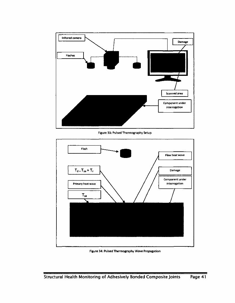
Infrared camera
Damage
Flashes
Component under
interrogation
Figure 33: Pulsed Thermography Setup
Flaw heat wave
Damage
Component under
interrogation Primary heat wave
Figure 34: Pulsed Thermography Wave Propagation
Structural Health Monitoring of Adhesively Bonded Composite Joints Page 41

There are two forms of thermography, Pulse (PT) and Lock-in (LT) [54,55,56]. PT is an analysis for
which the application of a single thermal unit pulse is applied and steady state temperature
response is captured using the infrared camera. LT is an analysis for which the application of
periodic heating is applied and the temperature profile is captured over a predefined time
window. Energy input plots as well as temperature responses for both PT and LT have been
presented within Figure 35.
PT requires less computational resources as compared to LT and it has the ability to detect
defects at different depths. Damage detection is done by comparing surface temperatures of
defective areas and defective-free areas. Two temperature profiles are captured using an
infrared camera, Tsa and Td, as shown in Figure 36. Tsa is the surface temperature of the defect
areas while Td is the surface temperature of defective areas. If a difference of Tso and Td (AT)
exist as shown in Figure 36, then the system indicates damage. The surface temperature for
defective areas is also affected by the depth of damage. Studies have shown that shallow
damages will yield a higher Td while deeper damages will yield a lower Td [54]. Experimental
analysis for a plate with multiple holes at different depths is shown in Figure 37(a); results of
which show that Td is a function of defect depth. However, the 2.0mm hole (top right corner)
appears to have a higher Td than that of the 1.5mm deep hole; this error is attributed to uneven
heating of the surface. Figure 37(b) shows the transient state results of the surface temperature;
from that image, it is clear that the surface is unevenly heated. Uneven heating is one of the
major drawbacks to PT as it leads to inadequate defect depth detection. Uneven heating may be
caused by a number of factors including wind and external lighting sources; this provides
additional difficulty in defect detection. For that reason, LT becomes useful [55].
Structural Health Monitoring of Adhesively Bonded Composite Joints Page 42
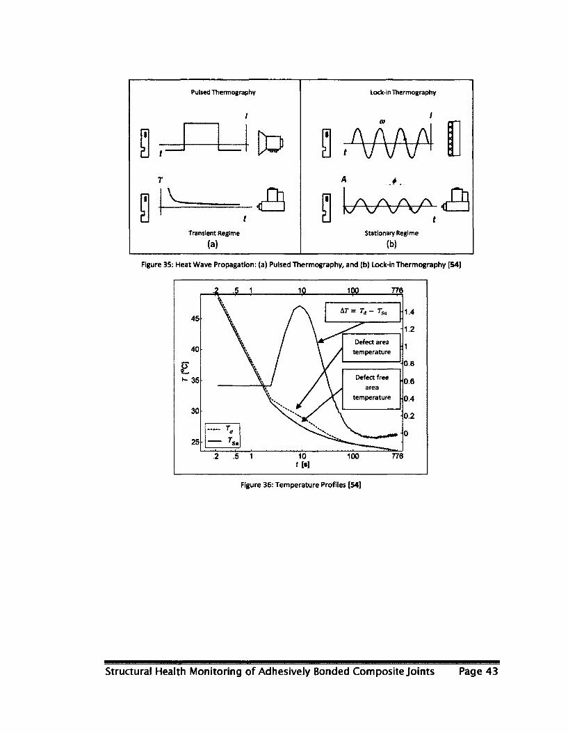
Pulsed Thermography Lock-in Thermography
to
Co 3 ,VW
V 9 t
Transient Regime
(a)
i/vw1 <5 t
Stationary Regime
(b)
Figure 35: Heat Wave Propagation: (a) Pulsed Thermography, and (b) Lock-in Thermography [54]
Defect area
temperature
Defect free
area
temperature
Figure 36: Temperature Profiles [54]
Structural Health Monitoring of Adhesively Bonded Composite Joints Page 43
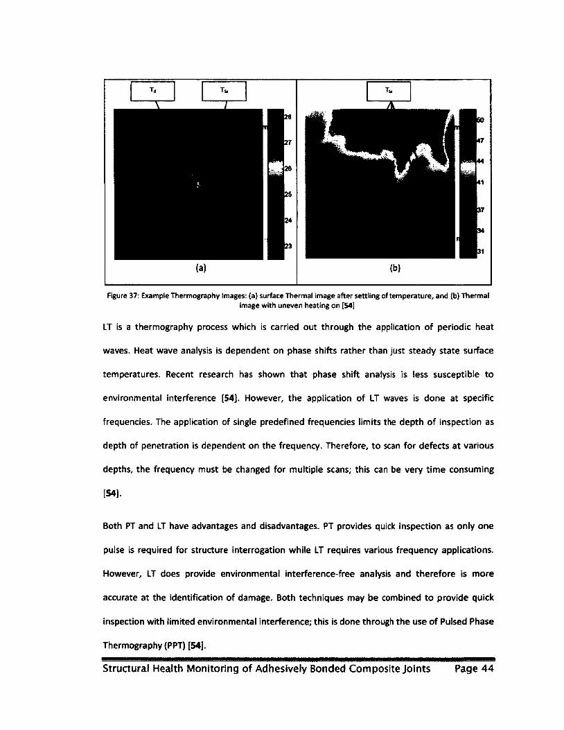
Figure 37: Example Thermography Images: (a) surface Thermal image after settling of temperature, and (b) Thermal image with uneven heating on [54]
LT is a thermography process which is carried out through the application of periodic heat
waves. Heat wave analysis is dependent on phase shifts rather than just steady state surface
temperatures. Recent research has shown that phase shift analysis is less susceptible to
environmental interference [54]. However, the application of LT waves is done at specific
frequencies. The application of single predefined frequencies limits the depth of inspection as
depth of penetration is dependent on the frequency. Therefore, to scan for defects at various
depths, the frequency must be changed for multiple scans; this can be very time consuming
[54].
Both PT and LT have advantages and disadvantages. PT provides quick inspection as only one
pulse is required for structure interrogation while LT requires various frequency applications.
However, LT does provide environmental interference-free analysis and therefore is more
accurate at the identification of damage. Both techniques may be combined to provide quick
inspection with limited environmental interference; this is done through the use of Pulsed Phase
Thermography (PPT) [54].
Structural Health Monitoring of Adhesively Bonded Composite Joints Page 44
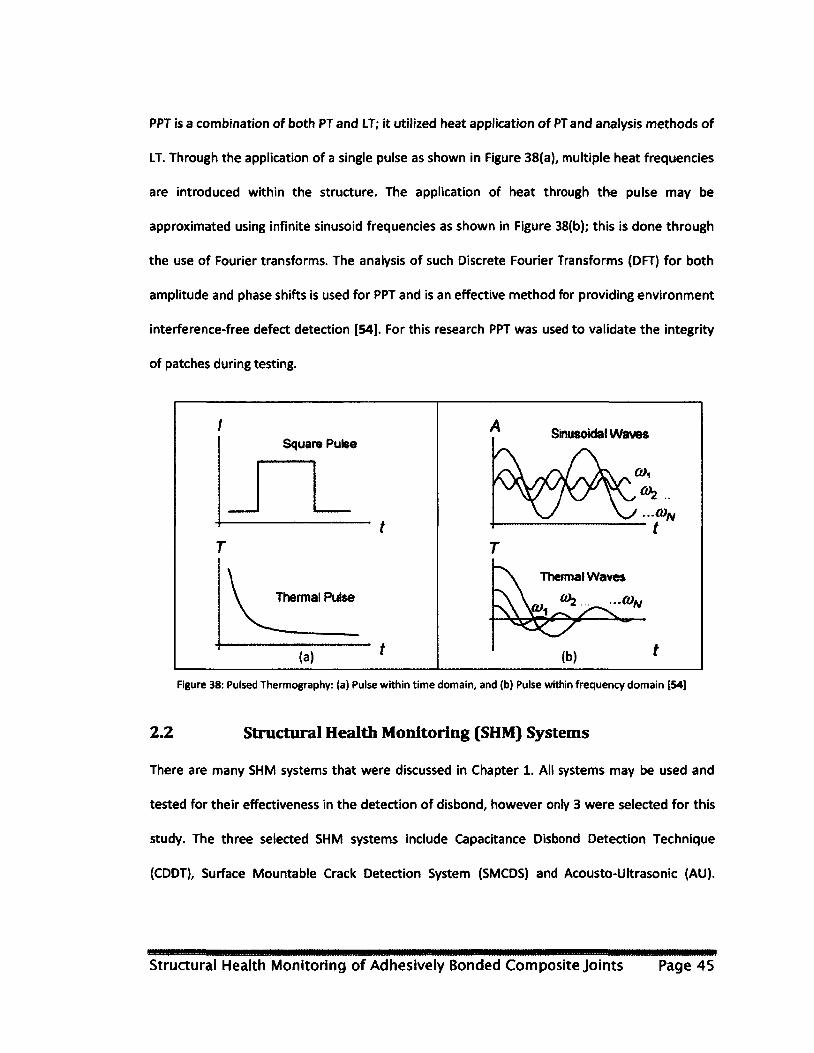
PPT is a combination of both PT and LT; it utilized heat application of PT and analysis methods of
LT. Through the application of a single pulse as shown in Figure 38(a), multiple heat frequencies
are introduced within the structure. The application of heat through the pulse may be
approximated using infinite sinusoid frequencies as shown in Figure 38(b); this is done through
the use of Fourier transforms. The analysis of such Discrete Fourier Transforms (DFT) for both
amplitude and phase shifts is used for PPT and is an effective method for providing environment
interference-free defect detection [54]. For this research PPT was used to validate the integrity
of patches during testing.
Sinusoidal Waves Square Pulse
T
Thermal Waves
Thermal Pulse xu.
Figure 38: Pulsed Thermography: (a) Pulse within time domain, and (b) Pulse within frequency domain [54]
2.2 Structural Health Monitoring (SHM) Systems
There are many SHM systems that were discussed in Chapter 1. All systems may be used and
tested for their effectiveness in the detection of disbond, however only 3 were selected for this
study. The three selected SHM systems include Capacitance Disbond Detection Technique
(CDDT), Surface Mountable Crack Detection System (SMCDS) and Acousto-Ultrasonic (AU).
Structural Health Monitoring of Adhesively Bonded Composite Joints Page 45

Other SHM technologies that have been described in section 1.2.2 have not been investigated in
this study for the flowing reasons:
• Fibre Bragg Gratings (FBG) and Strain Gauges (SG): SG was amongst the first
technologies to be utilized on patch bonded repairs [57]. Strain measurements have
been tested by many research institutions around the world and there are many
publications to support their findings. Research on the use of SG for SHM application
concludes that this technology works well. However, to fully monitor the entire area of
the patch, many strain gauges must be used. Strain gauges were not selected as
previous research has shown their effectiveness. Also, due to limited access to FBG
technology, this technology was not selected.
• Eddy Current (EC): EC technology works based on conduction properties of the
components being tested. For this study, composite materials are being utilized. Unlike
metallic materials, composites have no or very low conductive properties. For that
reason, EC sensors were not selected.
• Comparative Vacuum monitoring (CVM): CVM is similar to SMCDS and therefore only
one was chosen for this research. CVM is composed of small capillary tubes which are
monitored for leaks. These leaks are caused by crack nucleation and growth underneath
these capillary tubes. SMCDS is based on similar principle; however, rather than using
capillary tubes, the system uses conductive paint with low voltage. Electrical flow is
interrupted by the nucleation and growth of cracks through the conductive paint. Due
to their similarities, only SMCDS was chosen.
• Acoustic Emission: Acoustic Emission sensors and data acquisition systems were not
readily available.
Structural Health Monitoring of Adhesively Bonded Composite Joints Page 46

2.2.1 Capacitance Disbond Detection Technique (CDDT)
Capacitance Disbond Detection Technique (CDDT) has been utilized by the National Research
Council Canada (NRC) for the detection of disbond of a patch from a metallic substrate. Tests at
the NRC demonstrated that patch disbonds resulted in a drop of capacitance [48]. The following
section describes the physics behind the CDDT.
2.2.1.1 Basics of a capacitor
A capacitor is a device that stores energy in the form of a static electrical field. Electromagnetic
fields within a capacitor are created by allowing the formation of an electric potential
difference. The potential difference is the result of negative and positive charge build-up along
conductive plates which are separated by an insulating medium as show in Figure 39.
Capacitance is the measure of the ability of a capacitor to store energy and is measured in
Farads. Capacitance as shown in Equation 3 is the ratio of charge (Q) build-up to the applied
voltage (V). Capacitance can also be written in the form shown in Equation 4 [58,59].
_ (? Equation 3 V
_ KE0A Equation 4
~d~
Where: • K is the dielectric constant, • e0 is the permittivity of free space and eq = 8.854x10⁻¹² F/m, • A is the area of each of the parallel plates as shown in Figure 39, and • d is the separation distance between the conductive plates; this is also the thickness of
the isolating medium as shown in Figure 39.
Structural Health Monitoring of Adhesively Bonded Composite Joints Page 47

Conductive
plates
Electromagnetic
field
Current Area (A) Battery
\ /
Battery
tOICIOIOIOIO
EE SEE IOI
Charge buildup
(Q)
Distance
Insulating
medium
Figure 39: Basics of a Capacitor
In situations where the isolating layer remains unchanged, both K and e 0 from Equation 4
remain constant and therefore do not influence the capacitance of the system. In that specific
case, the area of the conductive plates and the separation distance will dominate the energy
carrying capacity of the capacitor.
Capacitor theory may be used for SHM of composite joints. This technology has the potential for
the detection of adhesive failure within metallic-to-metallic, composite-to-metallic and
composite-to-composite joints, provided that the components being joined are conductive.
Patch bonded repairs are the most basic form of joints that may be monitored using CDDT, as
the parallel plate capacitance equations hold. Figure 40 shows two joined components: a patch
and a substrate which are bonded using a film adhesive. Fully bonded joint capacitance can be
calculated using Equation 4: where K is equal to that of the relative static permittivity of the
adhesive and d is equal to the thickness of the adhesive denoted by db within the Magnification
A of Figure 40 [58,59]. Disbonded joint capacitance may be modeled using Equation 4; however,
in this case, there exist two relative static permittivity values; one for the adhesive and one for
Structural Health Monitoring of Adhesively Bonded Composite Joints Page 48
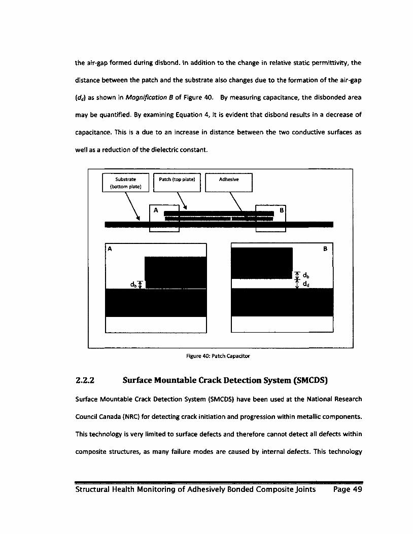
the air-gap formed during disbond. In addition to the change in relative static permittivity, the
distance between the patch and the substrate also changes due to the formation of the air-gap
(dd) as shown in Magnification B of Figure 40. By measuring capacitance, the disbonded area
may be quantified. By examining Equation 4, it is evident that disbond results in a decrease of
capacitance. This is a due to an increase in distance between the two conductive surfaces as
well as a reduction of the dielectric constant.
Substrate
(bottom plate)
Patch (top plate) Adhesive
Figure 40: Patch Capacitor
2.2.2 Surface Mountable Crack Detection System (SMCDS)
Surface Mountable Crack Detection System (SMCDS) have been used at the National Research
Council Canada (NRC) for detecting crack initiation and progression within metallic components.
This technology is very limited to surface defects and therefore cannot detect all defects within
composite structures, as many failure modes are caused by internal defects. This technology
Structural Health Monitoring of Adhesively Bonded Composite Joints Page 49
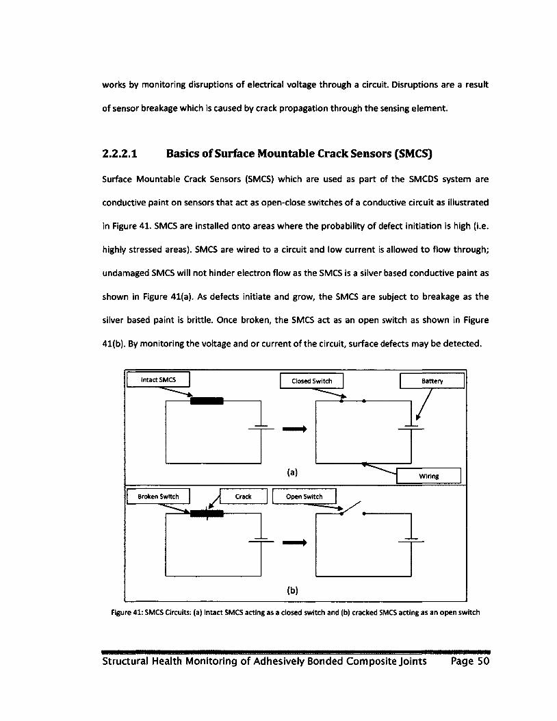
works by monitoring disruptions of electrical voltage through a circuit. Disruptions are a result
of sensor breakage which is caused by crack propagation through the sensing element.
2.2.2.1 Basics of Surface Mountable Crack Sensors (SMCS)
Surface Mountable Crack Sensors (SMCS) which are used as part of the SMCDS system are
conductive paint on sensors that act as open-close switches of a conductive circuit as illustrated
in Figure 41. SMCS are installed onto areas where the probability of defect initiation is high (i.e.
highly stressed areas). SMCS are wired to a circuit and low current is allowed to flow through;
undamaged SMCS will not hinder electron flow as the SMCS is a silver based conductive paint as
shown in Figure 41(a). As defects initiate and grow, the SMCS are subject to breakage as the
silver based paint is brittle. Once broken, the SMCS act as an open switch as shown in Figure
41(b). By monitoring the voltage and or current of the circuit, surface defects may be detected.
Crack Broken Switch
Intact SMCS Closed Switch Battery
Wiring
Open Switch
Figure 41: SMCS Circuits: (a) Intact SMCS acting as a closed switch and (b) cracked SMCS acting as an open switch
Structural Health Monitoring of Adhesively Bonded Composite Joints Page 50
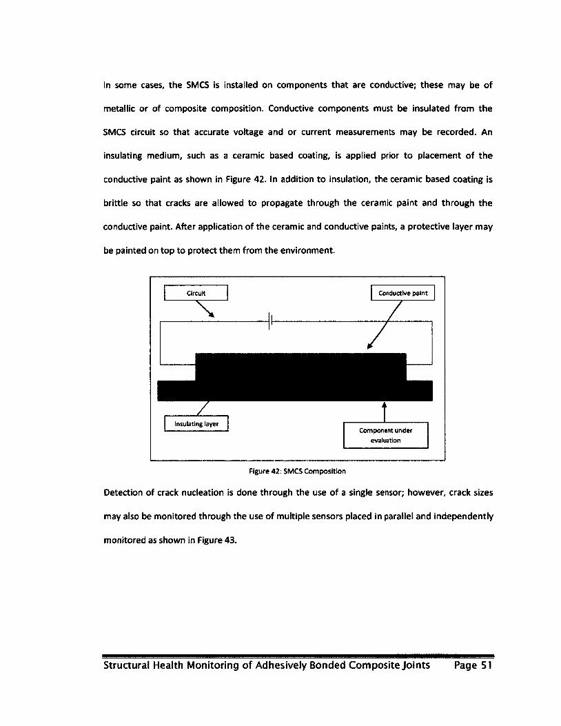
In some cases, the SMCS is installed on components that are conductive; these may be of
metallic or of composite composition. Conductive components must be insulated from the
SMCS circuit so that accurate voltage and or current measurements may be recorded. An
insulating medium, such as a ceramic based coating, is applied prior to placement of the
conductive paint as shown in Figure 42. In addition to insulation, the ceramic based coating is
brittle so that cracks are allowed to propagate through the ceramic paint and through the
conductive paint. After application of the ceramic and conductive paints, a protective layer may
be painted on top to protect them from the environment.
Circuit Conductive paint
Insulating layer Component under
evaluation
Figure 42: SMCS Composition
Detection of crack nucleation is done through the use of a single sensor; however, crack sizes
may also be monitored through the use of multiple sensors placed in parallel and independently
monitored as shown in Figure 43.
Structural Health Monitoring of Adhesively Bonded Composite Joints Page 51

Crack
Sensor 5
Sensor 4
Sensor 3
Sensor 2
Sensor 1
Figure 43: SMCS Placement
2.2.3 Acousto-Ultrasonic (AU)
Acousto-Ultrasonic is a method by which the integrity of a structure is investigated through the
propagation of ultrasonic waves. All materials have specific properties that change with the
introduction of damage. Wave propagation through materials is highly dependent on the
material's properties; changes in such properties leads to a change in signal propagation and
their responses. Changes of such signals may be correlated to damage [33,60,61].
There are many types of ultrasonic waves that exist within structures, all of which are classified
as elastic waves. One small subset of such waves are Lamb waves. Lamb waves are surface
guided waves that propagate over large distances and are less susceptible to large attenuation,
even in composite materials [32]. Lamb waves scatter as well as undergo modal conversion in
the presence of damage; this makes them suitable for damage detection. Analysis of lamb
waves have the capability of detecting disbonding, corrosion, cracking, holes, delamination,
broken fibres, resin cracks, inclusions and moisture ingression [33,62]. However, Lamb waves
exist in multiple modes, wave reflection and dispersion of such modes off boundaries makes it
Structural Health Monitoring of Adhesively Bonded Composite Joints Page 52

difficult to interpret damage as algorithms are frequency dependent [33,63]. In composites,
there exist two phases: a fibre and a matrix; Lamb waves interact with these two phases,
resulting in lots of signal dispersion and reflection, thus making it difficult to analyze the signals.
Lamb waves (LW) are known as guided waves, which are bounded between two free surfaces.
LW are elastic perturbations propagating within thin structures. The propagation of LW in a thin
structure along with the co-ordinate system is illustrated in Figure 44. The motion of the
particles in LW are in the direction of wave propagation and perpendicular to it. LW are
superposition of pressure waves (P-waves) and shear vertical waves (SV-waves). P-waves are
generated by applying normal forces along the Xj direction [Figure 45(a)]; whereas, SV-waves
are generated by applying shear forces along the x3 direction [Figure 45(b)]. The combination of
P and SV waves generate LW, which propagate in two different and independent modes, known
as symmetric (S„) and anti-symmetric (An). [33,63,64]
2.2.3.1 Basics of Lamb waves
Lamb wave
Figure 44: Co-ordinate System [33)
Structural Health Monitoring of Adhesively Bonded Composite Joints Page 53

Figure 45: Particle Motion within a Solid Medium: (a) particles subject to pressure force, and (b) particles subject to shear force [64]
Note: Detail derivation of LW equations is beyond the scope of this thesis; therefore only the
important steps for deriving the LW equations for isotropic materials are discussed. Einstein's
summation convention for tensor notation is used to show the derivation of LW equations. All
the following equations have been obtained through two primary sources [33,64].
The following steps are generally taken to derive the LW equations [64]:
Consider equation of motion using Newton's second law, which gives:
Equations
Where: • F is the force, • m is the mass,
Structural Health Monitoring of Adhesively Bonded Composite Joints Page 54

• a is the acceleration, and • / =1,2,3
Consider equation of motion using Newton's second law, which gives:
Where • cr is the stress, • A is the area, • t is the shear stress, and • N and T are subscripts denoting Normal and Tangential directions respectively
For a 3-D case, stresses can be written in the matrix form as:
Where • Ttj is the stress, • /= 1,2,3
• 7 = 1,2,3
• Eij is the strain,
• A is the lame constant and denoted by Equation 9 • 6 is the shear modulus, and
• Sjj is the Kronecker delta and denoted by Equation 10
Fn - a A ; Ft = rA Equation 6
Equation 7
Stresses can be related in tensor form in terms of strains as:
TtJ = Msn +e22 + e33)Sv + 2 Gsv Equation 8
Equation 9
Where
• E is Young's modulus, and • v is Possion's ratio
Structural Health Monitoring of Adhesively Bonded Composite Joints Page 55

Equation 10
Strains can be related to displacement using:
1 du, + dUj
u 2 dx dx v J ' J
Equation 11
Where:
• u is the displacement and • x is the direction
To understand LW, one must first examine the motion of particles within a material. Equation 5
through Equation 10 will be used in the following steps to evaluate how particles behave in the
presence of applied forces.
Consider an infinitesimal element as shown in Figure 46:
Structural Health Monitoring of Adhesively Bonded Composite Joints Page 56
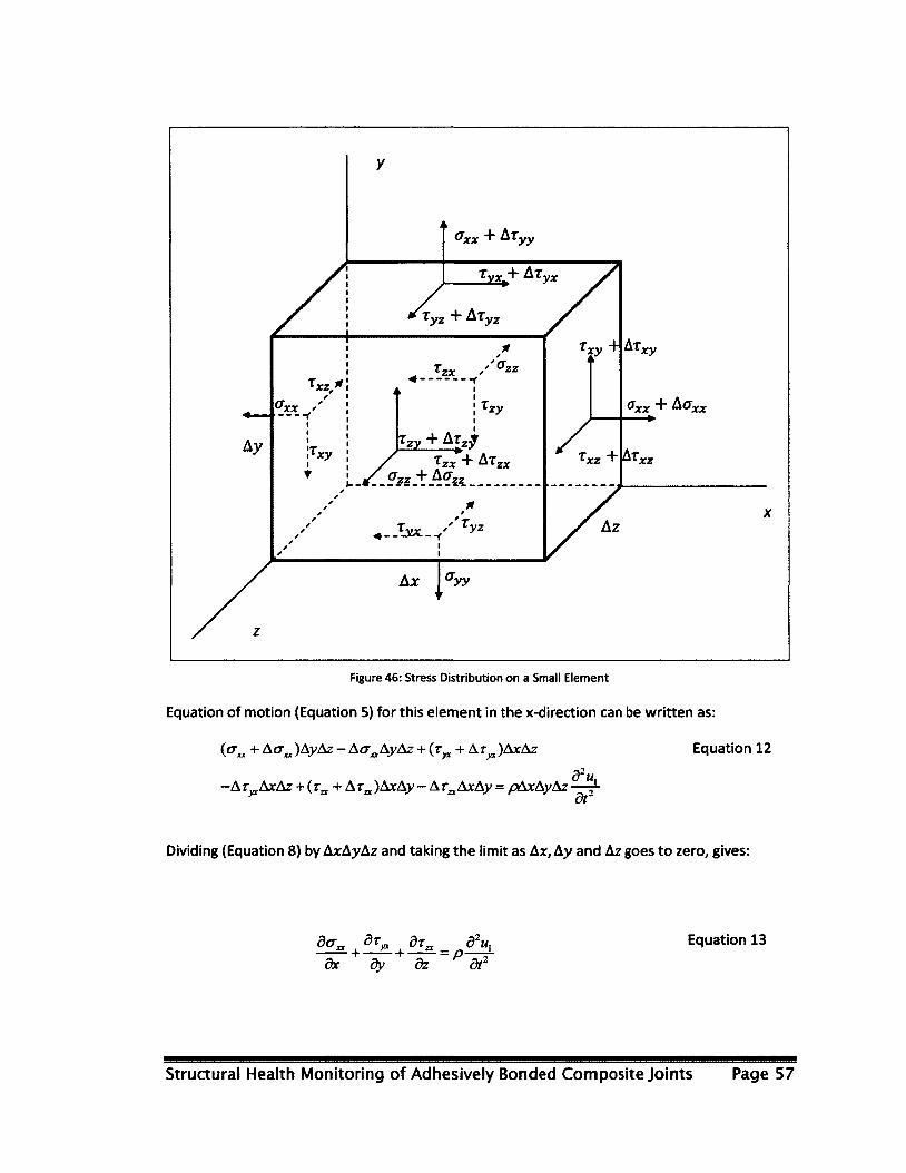
yz
xy xy 'zz zx
XZ.
xz
Az yz
yy
Figure 46: Stress Distribution on a Small Element
Equation of motion (Equation 5) for this element in the x-direction can be written as:
(o^ + Acrxt)AyAz - A<JaAyAz + (r^ + AT )AxAz Equation 12
-ATyxAxAz + (T2x+ATzx)AxAy-ATzxAxAy = pAxAyAz 2 d\
dt2
Dividing (Equation 8) by AxAyAz and taking the limit as Ax, Ay and Az goes to zero, gives:
5cr dr dr d\ Equation 13 ——+—^- + —p—r-
dx dy dz dt
Structural Health Monitoring of Adhesively Bonded Composite Joints Page 57

Where: • p is the material density
Equation of motion for y- and z-direction can be generated in a similar fashion
Substituting the stress (Equation 8) into Equation 13 yields:
[-£(£•,, +£22 +£33)^ -+"2C?£-y]-t- ——-[/l(£u +e22 +£33)3, +2Ge iJ~] 2 dx}
L 11 " " y ,JJ dx.
+—[ A(st ,+s22 + £33 )Sy + 2Gsij ] = p-̂ r
Through manipulation, Equation 14 can be further reduced into Equation 15 and consequently
into Equation 16.
d d d V . . _ _ 8\ Equation 15
^+a^+a^JA(til +£a+£")S»+2Gs"]'pP"
, x d2u Equation 16 V(Meu +e22 +£33)^ +2Ge l )) = p-j-
The equation of motion (Equation 16) can be written using Equation 11 in terms of displacement
as:
(x+G)-^S-+G-^-=p^Ui Equa,ion17
dx,dxj dXjdXj dt
From Equation 17, the general longitudinal wave equation can be written as:
d\ __}_d\ Equation 18
dx2 c2 dt2 I L
Where:
• L = P-wave speed and is given by Equation 19 n 1 . -«^\V/2
( A + 2 G )
P
Equation 19
Similarly, the general transverse wave equation can be written as:
Structural Health Monitoring of Adhesively Bonded Composite Joints Page 58

d\ _±_d\ Equation 20
dx2 cl dt2
Where:
• cT- shear or S-wave velocity and is given by Equation 21:
c J£f I p,
Equation 21
Lamb wave equations are generated assuming that motion depends only on xx and x3
directions.
Using the Helmholtz decomposition in which a three-dimensional displacement vector can be
decomposed into a sum of curl-free and divergence-free vector field, the displacement vector
can be written as:
u = V# + Vxip Equation 22
Where:
• <j> is the scalar function and • X/J is the vector function. Both of which will be computed at later stages within the
derivation.
The displacement vector u, can be expanded as:
dd 86 dw., - du/, - Equation 23 u =—— h—— —e. +——e,
dxj dxj dx3 dx,
Equation 23 can be simplified in terms of individual displacements as:
_ d$ dy/2 Equation 24 1 Sx, dx3
u2=0
dd> du/7 w, = — — Sx3 fic,
The governing longitudinal wave equation (Equation 18) in terms <p can be written as:
Structural Health Monitoring of Adhesively Bonded Composite Joints Page 59

ay i ay Sx,2 dxj c\ dt2
Equation 25
Similarly, the governing transverse wave equation (Equation 20) in terms of xp can be written as:
ay ay 1 ay dx; dx2 c\ dt2
Equation 26
Solutions to the scalar and vector functions may be obtained by assuming the following
functions:
0 = [A, sin (px3 ) + A2 COS (px3 )]E /(fo.-a*) Equation 27
¥ = [A sin(^c3) + B2 cos(qt*3 )]e i(bcx-wl) Equation 28
Where: • co is the angular frequency, • Ms time, • k is the circular wave number, • AH A& BH B2 are all constants determined by the boundary conditions, and • p and q are equal to Equation 29 and Equation 30, respectively.
P2 =
( 2 \ m -k 2
c2 , v l y
Equation 29
f 2
— -k 2 JZ K
Equation 30
Substituting Equation 27 and Equation 28 into Equation 24, displacements can be written as:
m, = ik\_A, sin(/a3) + A, cos(/*3 + [qB, cos(qx3)-qB2 sin(qx3Equation 31
u3 = \_pA ̂cos (px3) - pAj sin (px})] e'(a*~fal} - ik [5, sin (qx3 ) + B2 cos (qx3)] e'( <a~kx')
Substituting the displacements (Equation 31) into Equation 8, the stresses can be written as:
^ 2ik[pA icos(px3)~ pA^sin^px-^ + tf^Bi sin (gx,) + B2 cos(qx3)] +^1 Equation 32 a3, =Ge'(b'-" , )
sin (qx3 )-q2B2 cos (qx,)]
Structural Health Monitoring of Adhesively Bonded Composite Joints Page 60
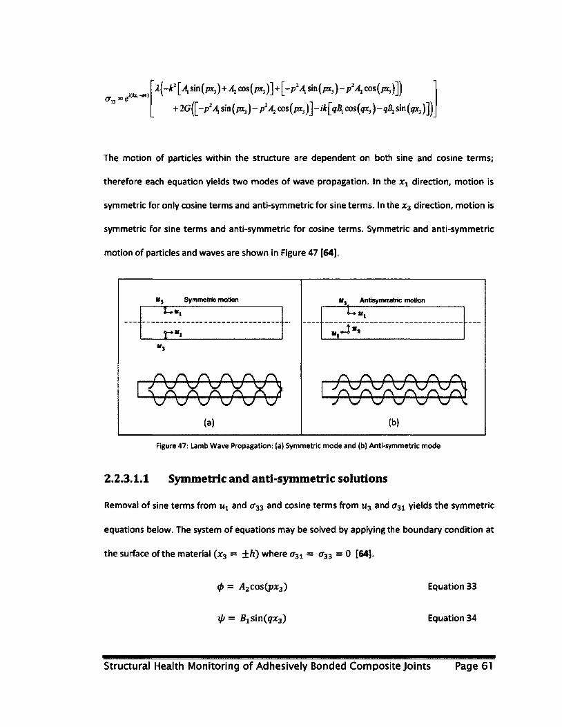
A(-*2 [4 sin (/BCj) + 4 cos(/*3)]+[~/>24 sin (px3) - p% cos(/a,)])
+2 G([-p24 »n (/^ ) - p24 cos(px3)] - ik [qBx cos (gx,) - qBt sin (?x,)])
The motion of particles within the structure are dependent on both sine and cosine terms;
therefore each equation yields two modes of wave propagation. In the xx direction, motion is
symmetric for only cosine terms and anti-symmetric for sine terms. In the x3 direction, motion is
symmetric for sine terms and anti-symmetric for cosine terms. Symmetric and anti-symmetric
motion of particles and waves are shown in Figure 47 [64].
u33 C
U) Symmetric motion
I-**,
(a)
If, Antisymmetric motion
AAAAAA
(W
Figure 47: Lamb Wave Propagation: (a) Symmetric mode and (b) Anti-symmetric mode
2.2.3.1.1 Symmetric and anti-symmetric solutions
Removal of sine terms from and «r33 and cosine terms from u3 and a31 yields the symmetric
equations below. The system of equations may be solved by applying the boundary condition at
the surface of the material (x3 = ±h) where a31 = a33 = 0 [64].
<f> = A2cos(px3) Equation 33
xp = B1s\r\{qx2) Equation 34
Structural Health Monitoring of Adhesively Bonded Composite Joints Page 61

ui = [?®i cos(qx3) + ikA2 cospx3]
u3 = -[ifcBiSinCqXa) + pA2 sin(px3)]
«r3i = G[—2ikpA2 sin(px3) + (k2 - q2)Bt sin(qx3)]
<r33 = -\k2A2 cos(px3) - Ap2i42 cos(px3)
— 2Gp2i42 cos(px3) — 2GikqB1 cos(gx3)
Equation 35
Equation 36
Equation 37
Equation 38
By equating Equation 37 and Equation 38 to zero as per the surface boundary conditions, a
solution for the equations may be identified. The non-trivial solution for the system of equations
then becomes Equation 39 [64].
tan(g/i) —4 k2pq Equation 39
tan(p/i) (q2 — k2)
Using the same approach and same surface boundary conditions, the anti-symmetric solution to
the following equations may be obtained [64].
0 = i41sin(p*3)
xf}= B2cos(qx3)
u t = [ikA-L sin(px3) — pB2 sin(gx3)]
«3 = [pAi cos(px3) - ikB2 cos qx3]
a31 = GftikpA! cos(px3) +(fe2 — q2)B2 cos(qx3)]
Equation 40
Equation 41
Equation 42
Equation 43
Equation 44
Structural Health Monitoring of Adhesively Bonded Composite Joints Page 62

°33 = — sin(px3) — XpzA1 sin(px3) — 2GpzA l sin(px3)
+ 2GikqB2 sin(gx3)
Equation 45
The non-trivial solution to this system of equations yields Equation 46.
tan(<j/i) _ (q2 — fc2)
tan(p/i) 4 k2pq
Equation 46
2.2.3.1.2 Numerical solution to Lamb wave equations
When considering only positive roots of the wave number (k), both Equation 39 and Equation 46
can be solved numerically by initially guessing a frequency, a phase velocity (Equation 47) and by
following steps as outlined in [64,65].
Following these steps yields dispersion curves as shown in Figure 48. Dispersion curves are
important for determining the frequency at which a material is to be interrogated. At minimum,
two modes will exist simultaneously and those correspond to A0 and S0 which are to the left of
the line as shown in Figure 48. Excitation at higher frequencies yields additional modes
A0,Ax,A2,....An and their associated symmetric modes. The presence of additional modes
makes for difficult analysis of the signal.
avg Equation 47
Structural Health Monitoring of Adhesively Bonded Composite Joints Page 63
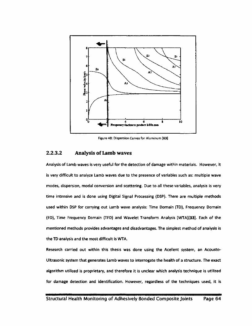
s \ ' \ \ ' \ \
7 Kv 6
m
Is
So
«•
JU s k jjj
> Al !
I
^ 2 4 6 S 10 Frcqococy tiackne^: pnxJocr
Figure 48: Dispersion Curves for Aluminum [63]
2.2.3.2 Analysis of Lamb waves
Analysis of Lamb waves is very useful for the detection of damage within materials. However, it
is very difficult to analyze Lamb waves due to the presence of variables such as: multiple wave
modes, dispersion, modal conversion and scattering. Due to all these variables, analysis is very
time intensive and is done using Digital Signal Processing (DSP). There are multiple methods
used within DSP for carrying out Lamb wave analysis: Time Domain (TD), Frequency Domain
(FD), Time Frequency Domain (TFD) and Wavelet Transform Analysis (WTA)[33]. Each of the
mentioned methods provides advantages and disadvantages. The simplest method of analysis is
the TD analysis and the most difficult is WTA.
Research carried out within this thesis was done using the Acellent system, an Acousto-
Ultrasonic system that generates Lamb waves to interrogate the health of a structure. The exact
algorithm utilized is proprietary, and therefore it is unclear which analysis technique is utilized
for damage detection and identification. However, regardless of the techniques used, it is
Structural Health Monitoring of Adhesively Bonded Composite Joints Page 64
known through paper findings in the literature that the Acellent software quantifies damage
using a Damage Index (Dl) [66]. For that reason, not all analysis techniques have been described
in detail, with the exception of TD analysis which is described in section 2.2.3.2.1.
2.2.3.2.1 Time Domain (TD) analysis
All transmitted and received signals are captured within the TD; hence, TD analysis is an ideal
starting point for data reduction.
Lamb waves, like all other waves, transport energy form one location to the next; presence of
damage changes the total energy being transported. TD analysis can therefore be applied to the
total energy of the signal for the identification of damage. Analysis of energy can be done using
the Hilbert transform [32,33]. The Hilbert transform is a method which looks at rapid changes in
frequency of the transmitted signal. The change in frequency may be correlated to damage or
the presence of other foreign objects. Figure 49(a) shows a Lamb wave signal for a damaged
aluminum plate while Figure 49(b) shows the Hilbert transform of the same signal. The Hilbert
transform in Figure 49(b) indicates a rapid change in frequency of the Lamb wave. This change in
frequency may be due to the presence of damage; however, it is hard to determine if this is due
to damage or due to other phenomena that may have existed since the manufacturing of the
component. To limit the effect of wall reflection and other phenomena that may influence the
results, a comparison of the current signal is made to a benchmark signal.
Structural Health Monitoring of Adhesively Bonded Composite Joints Page 65
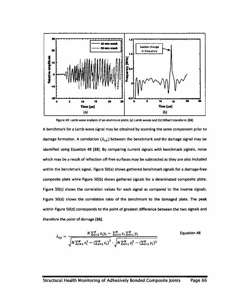
90 mm crack
Tim* [its]
Sudden change
in frequency
lime [y»]
Figure 49: Lamb wave analysis of an aluminum plate: (a) Lamb waves and (b) Hilbert transform [32]
A benchmark for a Lamb wave signal may be obtained by scanning the same component prior to
damage formation. A correlation (A^,) between the benchmark and the damage signal may be
identified using Equation 48 [33]. By comparing current signals with benchmark signals, noise
which may be a result of reflection off free surfaces may be subtracted as they are also included
within the benchmark signal. Figure 50(a) shows gathered benchmark signals for a damage-free
composite plate while Figure 50(b) shows gathered signals for a delaminated composite plate.
Figure 50(c) shows the correlation values for each signal as compared to the inverse signals.
Figure 50(d) shows the correlation ratio of the benchmark to the damaged plate. The peak
within Figure 50(d) corresponds to the point of greatest difference between the two signals and
therefore the point of damage [33].
XX y —
N xc/i - Xi=xxt liLi yt Equation 48
a , - a s . . * ) 2 • I ? . , y ? - a s , , > , y
Structural Health Monitoring of Adhesively Bonded Composite Joints Page 66
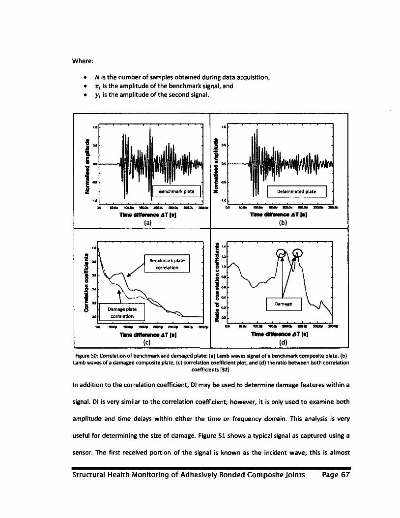
Where:
• N is the number of samples obtained during data acquisition, • xi is the amplitude of the benchmark signal, and • yi is the amplitude of the second signal.
Benchmark plate
ao aoou mm snoou soot ao&ou aaoov Time (Utterance 4T{*]
(a)
Delaminatea plate
ao wAt tana*
TteMdm«ranc0iST (•] (b)
Benchmark plate
correlation
Damage plate
correlation
Damage
00 9QHM tooop 1«C* 200C|t MM* 30051* 3»<|l TIiiw diff«ranc«4T [•]
(c)
BLOy lOOty ttO* SKU|I Sttflp ME ftp Time dlfterenc* AT [s]
(d)
Figure 50: Correlation of benchmark and damaged plate: (a) Lamb waves signal of a benchmark composite plate, (b) Lamb waves of a damaged composite plate, (c) correlation coefficient plot, and (d) the ratio between both correlation
coefficients [32]
In addition to the correlation coefficient, Dl may be used to determine damage features within a
signal. Dl is very similar to the correlation coefficient; however, it is only used to examine both
amplitude and time delays within either the time or frequency domain. This analysis is very
useful for determining the size of damage. Figure 51 shows a typical signal as captured using a
sensor. The first received portion of the signal is known as the incident wave; this is almost
Structural Health Monitoring of Adhesively Bonded Composite Joints Page 67

identical to the transmitted signal with the exception of amplitude change. The second portion
is the scattered damage wave; this wave is a result of interference between the incident wave
and damage. Two signals captured at two different states may be correlated to each other using
the 01 (Equation 49).
Dl = (Apt — Ap2) x (Ti — T2) Equation 49
Where:
• Ap is the amplitude • T is the difference of ToF • The subscripts 1 & 2 denote two signal states, one of which may be the benchmark
state.
DIs are scalar values which are obtained by comparing two current signals to each other or
against a benchmark signal. Assignment of known damage size to the calculated Dl correlates
damage growth with changes in Dl. Therefore, databases within data reduction algorithms may
be developed to contain all calculated Dl with their associated damage size. Newly calculated Dl
may be compared to those within the database to interpret damage size.
Structural Health Monitoring of Adhesively Bonded Composite Joints Page 68
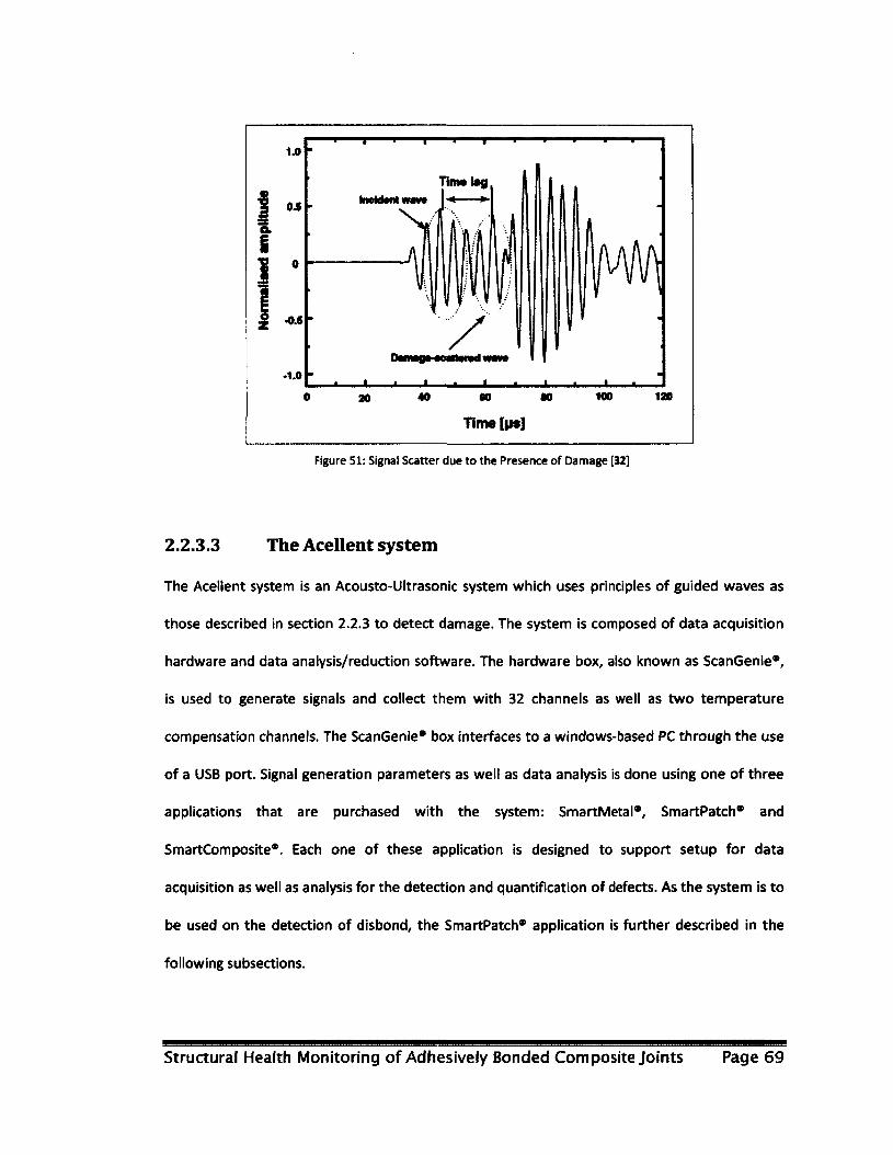
1.0
04
Ob i ? •
£ -0.5
-1.0
• I I I I I
Tinwlag
lr
i i i 20 40 SO 80
Time [in]
100 120
Figure 51: Signal Scatter due to the Presence of Damage [32]
2.2.3.3 The Acellent system
The Acellent system is an Acousto-llltrasonic system which uses principles of guided waves as
those described in section 2.2.3 to detect damage. The system is composed of data acquisition
hardware and data analysis/reduction software. The hardware box, also known as ScanGenie*,
is used to generate signals and collect them with 32 channels as well as two temperature
compensation channels. The ScanGenie* box interfaces to a windows-based PC through the use
of a USB port. Signal generation parameters as well as data analysis is done using one of three
applications that are purchased with the system: SmartMetal*, SmartPatch* and
SmartComposite®. Each one of these application is designed to support setup for data
acquisition as well as analysis for the detection and quantification of defects. As the system is to
be used on the detection of disbond, the SmartPatch* application is further described in the
following subsections.
Structural Health Monitoring of Adhesively Bonded Composite Joints Page 69

2.2.3.3.1 SmartPatch® application setup
The SmartPatch* application provides three purposes: system setup, defect detection and
defect quantification. Every component being tested using this system requires an independent
setup, regardless of similarities. In cases where coupons have identical geometry and sensor
placements, setup files will be similar but not identical.
Creation of a new test starts with the setup of sensor locations; this can be done by creating a
new sensor layout, or by utilizing a previously used layout as shown in Figure 52(a). Setup of
sensors is done using a Cartesian coordinate system. A point on the coupon must be set to the
(0, 0) position. The exact location of the (0, 0) point is not critical, as the purpose of this step is
to identify the location of each sensor with respect to the location of all other sensors. These
coordinates are used for the determination of signal ToF. Figure 52(b) shows the setup of
sensors, the number of sensors installed on the component, the number of smart layers, and
the unit of measurement which appear in the left hand side of the figure. The analysis of two or
more independent components can be done simultaneously by assigning multiple smart layers;
this is only done when signals form one layer is known not to affect the other layer. The number
of smart layers is always set to the value 1 for all experiments carried out for this research.
Figure 53(a) and Figure 53(b) show a single and double smart layer setup, respectively.
Structural Health Monitoring of Adhesively Bonded Composite Joints Page 70
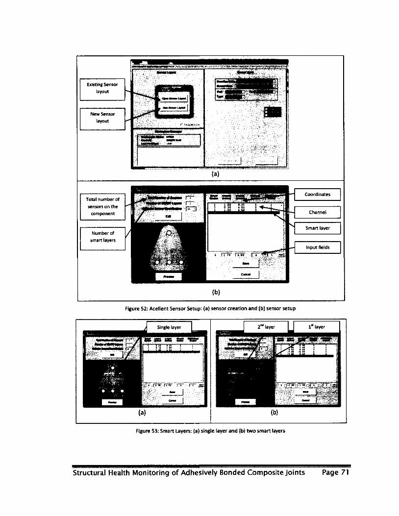
Existing Sensor
layout
New Sensor
layout
w/mm*
(a)
Total number of
sensors on the
component
Number of
smart layers
F~3
o-
£S - - -1 to t 1.2$ 1 ' 1 2 0 30 t SO 2 1
4 HTTT fTsT pr*| 9mm j-
Canal j
i «j
(b)
Coordinates
Channel
Smart layer
Input fields
Figure 52: Acellent Sensor Setup: (a) sensor creation and (b) sensor setup
Single layer
Figure 53: Smart layers: (a) single layer and (b) two smart layers
Structural Health Monitoring of Adhesively Bonded Composite Joints Page 71
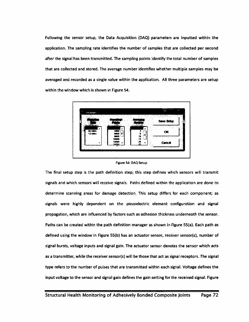
Following the sensor setup, the Data Acquisition (DAQ) parameters are inputted within the
application. The sampling rate identifies the number of samples that are collected per second
after the signal has been transmitted. The sampling points identify the total number of samples
that are collected and stored. The average number identifies whether multiple samples may be
averaged and recorded as a single value within the application. All three parameters are setup
within the window which is shown in Figure 54.
Figure 54: DAQ Setup
The final setup step is the path definition step; this step defines which sensors will transmit
signals and which sensors will receive signals. Paths defined within the application are done to
determine scanning areas for damage detection. This setup differs for each component; as
signals were highly dependent on the piezoelectric element configuration and signal
propagation, which are influenced by factors such as adhesion thickness underneath the sensor.
Paths can be created within the path definition manager as shown in Figure 55(a). Each path as
defined using the window in Figure 55(b) has an actuator sensor, receiver sensor(s), number of
signal bursts, voltage inputs and signal gain. The actuator sensor denotes the sensor which acts
as a transmitter, while the receiver sensor(s) will be those that act as signal receptors. The signal
type refers to the number of pulses that are transmitted within each signal. Voltage defines the
input voltage to the sensor and signal gain defines the gain setting for the received signal. Figure
Structural Health Monitoring of Adhesively Bonded Composite Joints Page 72
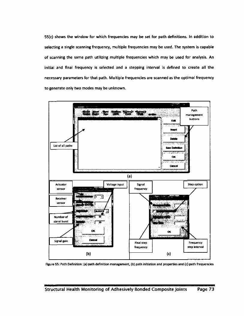
55(c) shows the window for which frequencies may be set for path definitions. In addition to
selecting a single scanning frequency, multiple frequencies may be used. The system is capable
of scanning the same path utilizing multiple frequencies which may be used for analysis. An
initial and final frequency is selected and a stepping interval is defined to create all the
necessary parameters for that path. Multiple frequencies are scanned as the optimal frequency
to generate only two modes may be unknown.
Path
management
buttons
*SBS3r..
List of all paths Sm DefMnon
Voltage input Signal
frequency
Step option Actuator
sensor
Receiver
sensor
Number of
signal burst
Signal gain Frequency
step interval
Final step
frequency
Figure 55: Path Definition: (a) path definition management, (b) path initiation and properties and (c) path frequencies
Structural Health Monitoring of Adhesively Bonded Composite Joints Page 73

After path definition, a benchmark reading is acquired, similar to that shown in Figure 56(a).
Gains within the path definition were individually adjusted so that the bursts 6-10 are between
0.5V and l.OV as shown in Figure 56(b). Setting gains so that voltage is between 0.5V and l.OV
ensures that energy drops may be correlated to a specific damage size. The system is now ready
for data acquisition and new readings are taken using the "take new data" button as shown in
Figure 57.
Signal not within limits (bursts 6-10)
Signal within limits
Cross Talk Cross Talk
90 100 190 300 250 300 350 T«iw(p*«c)
Figure 56: Signal Propagation Settings
Figure 57: SmartPatch* Main Window
Structural Health Monitoring of Adhesively Bonded Composite Joints Page 74

2.2.3.3.2 The Acellent system analysis
Signals acquired using the SmartPatch* application are analyzed using two built-in utilities, one
for the detection of damage and the second for the quantification. Detection of damage is done
using the Direct Path Image (DPI) utility, while the quantification of damage is done using the
Semi-Empirical Damage Sizing (SEDS) utility. Figure 58 shows an example of a coupon being
analyzed using the DPI. Within the figure, a digital representation of the coupon is shown with
all installed sensors. Paths which were scanned during the data acquisition step are analyzed
within the software to produce images for defect identification. Damage is indicated on the
digital representation images as shown in Figure 58. The intensity of damage may be evaluated
using the threshold value. The threshold correlates signal amplitude (i.e. energy) changes to the
application's color scale. Adjusting the threshold to a high value will only display changes in
signals that are very large while a low threshold will display almost all signal amplitude changes.
This is the reason for which the benchmark reading was setup so that bursts 6-10 are between
0.5V and l.OV. Additional analysis may be carried out on different portions of the signal by
adjusting the time window shown in Figure 58. However, for all analysis within this research, the
signal is truncated to only contain burst 6-10, as signal reflection from component edges should
not be included within the analysis.
Structural Health Monitoring of Adhesively Bonded Composite Joints Page 75
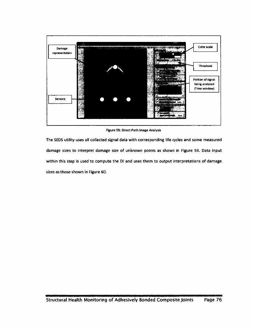
Damage
representation
Threshold
Portion of signal
being analyzed
(Time window)
Figure 58: Direct Path Image Analysis
The SEDS utility uses all collected signal data with corresponding life cycles and some measured
damage sizes to interpret damage size of unknown points as shown in Figure 59. Data input
within this step is used to compute the Dl and uses them to output interpretations of damage
sizes as those shown in Figure 60.
Structural Health Monitoring of Adhesively Bonded Composite Joints Page 76
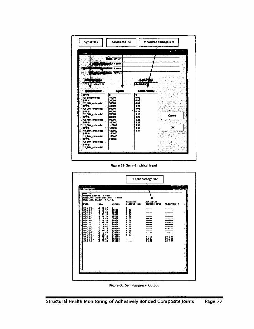
Signal files Associated life Measured damage size
mmrnmm| J9PP3-1
|5PP3-Jz oapawOa
8PP3- 0 0 i3LbmMnf.oot 10000 002 8PP3- 20000 002 12_10K_cyd«s<ttt 30000 004 8PP3- 40000 006 12_2OK_eyeto0at 50000 006 SPP3- 00000 014
70000 0.18 SPP3- 80000 0.22 12w40Kj*6#«.d* 90000 0.25 8PP3- 100000 0.29 12.90K.cydM.<M 110000 031 8PP3- 120000 0.33 l2_60K.cyd66.46t 130000 037 SPP3- 140000 12_70K.eydts.dX 190000 9#*P3- 200000 12_WK_<*<*t«.<J«t SPPJ-12.90K.9dM.tfat
Cancel
OK
Figure 59: Semi-Empirical Input
Output damage size
SFP3-12 Bw>ier Syitn Spciw Cent ifforation 4 SfwciMKt hater SPPM2
EaUMtad dtsbond «m
12 04 19 07/20/11 32 37 07/20/11
15 28 09 07/26/11 15 $0 3? 07/20/11 16 34 51 67/28/11 17 14:44 07/20/11 17 59 39 07/26/11 11 35 33 07/21/11 12 12 01 07/21/11 13 10 05 07/21/11 13 57 14 07/21/11 14 37 10 07/21/11 IS 12 53 07/21/11 15 40 5! 07/21/11 1* 23 32 07/21/11 It 50 57 07/21/11 15 29 40 07/22/11
0 10000 20000 30000 40000 50000 60000 70000 90000 90000 100000 110000 120000 130000 140000 ISOOOO 200000
0 0 02 0 02 0 04 0 06 0 08 0 14 0 10 0 22 0 25 0 29 0 31 0 33 0 37
0 456 0 509 0 691
tO 194 ±0 209 ±0 307
Figure 60: Semi-Empirical Output
Strurtural Health Monitoring of Adhesively Bonded Composite Joints Page 77

Chapter 3.0: Test Design and Coupon Manufacturing
Structural Health Monitoring (SHM) has been researched for many years. There are many SHM
systems available; however, some are more effective for detection of certain damage modes as
compared to others. The objective of this thesis was to test readily available SHM solutions for
the detection and quantification of crack growth as well as disbond. Testing the SHM system for
the detection of both crack growth and disbond required the development of different coupons
as well as test plans.
Three different types of coupons were developed to test the effectiveness of three SHM systems
for the detection and quantification of crack growth as well as disbond. The first type of coupons
was of metallic construction with a center surface crack; they were designed so that the SHM
systems may be used for the detection and quantification of crack growth. The second type of
coupons was of composite patches bonded to a metallic substrate design; they were designed
so that the SHM systems may be evaluated for the detection and quantification of both crack
and disbond growth. The third type of coupon consisted of composite patches bonded to a
composite substrate design; they were designed so that the SHM systems may be evaluated for
the detection and quantification of disbond growth.
This chapter is divided into three subsections: coupon design, coupon manufacturing and
coupon instrumentation.
3.1 Coupons
All three sets of coupons were manufactured using different processes as each set was
composed of different materials and had different requirements. Metallic and composite-to--
metallic coupons were designed and manufactured during earlier stages of the Smart Patch
Structural Health Monitoring of Adhesively Bonded Composite Joints Page 78
Project (prior to the start of this thesis project) [29,39] and therefore in-depth design and
manufacturing processes are not included within this chapter.
3.1.1 Metallic Coupons (Coupon Set 1)
Metallic coupons measuring 15.0 x 2.0 x 0.25 inches were manufactured of 2024-T3 aluminum.
These coupons were designed to determine the effectiveness of SHM systems for the detection
and quantification of cracks within metallic components. The dimensions for these coupons
were chosen so that internal stresses of the coupon did not exceed their yield strength (40 KSI);
this correlates to a static load of 20,000 lb.
All metallic coupons were initially machined with a rib along the length of the coupon as shown
in Figure 61. An Electronic Discharge Machining (EDM) notch was created at the surface of the
rib so that crack nucleation and propagation is allowed during fatigue of the coupons. Coupons
were fatigued until cracks for all coupons grew through the rib and into the aluminum substrate
as shown in Figure 62. Cracks were allowed to grow until surface cracks were approximately
0.20 inches in length as shown in Figure 62(a). Ribs were machined and the cracks were left
exposed as shown in Figure 62(b). To grow cracks, coupons were fatigued at maximum load of
13,000 lb (26 KSI) and minimum load of 1,300 lb (2.6 KSI) [39]. Surface Mountable Crack Sensors
(SMCS) were employed around the rib as shown in Figure 62(c) so that upon crack growth
through the rib and into the substrate, the SMCS would trip and fatigue cycles would stop. This
was done to limit surface crack lengths to approximately 0.25 inches. To obtain the final
measurement of crack lengths, ultrasound, eddy current and a travelling microscope were
utilized [39].
Structural Health Monitoring of Adhesively Bonded Composite Joints Page 79
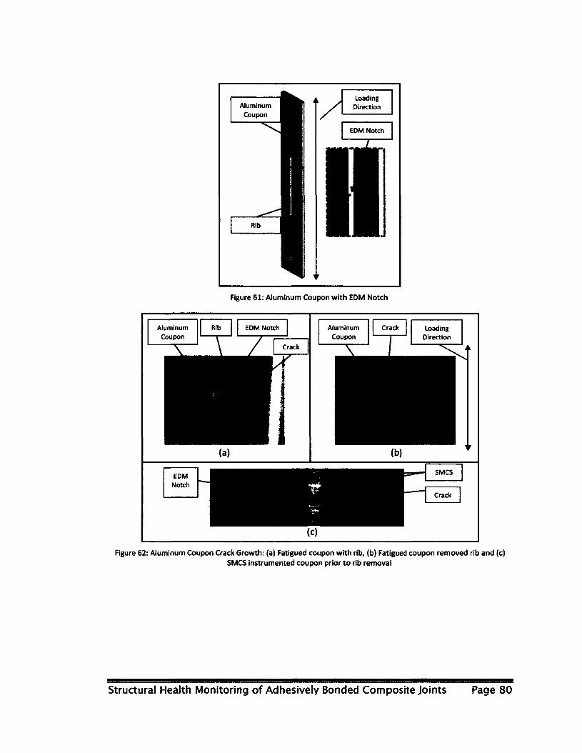
Figure 61: Aluminum Coupon with EDM Notch
Aluminum Coupon
EDM Notch Aluminum Coupon
Loading Direction
SMCS EDM Notch
Figure 62: Aluminum Coupon Crack Growth: (a) Fatigued coupon with rib, (b) Fatigued coupon removed rib and (c) SMCS instrumented coupon prior to rib removal
Structural Health Monitoring of Adhesively Bonded Composite Joints Page 80

3.1.2 Patched Metallic Coupons (Coupon Set 2)
Metallic coupons measuring 15.0 x 2.0 x 0.25 inches manufactured of 2024-T3 aluminum and
carbon fibre patches (doubters) measuring 5.0 x 2.0 inches were manufactured and are shown in
Figure 63(a) and Figure 63(b). In addition to the patch shown in Figure 63(b), a rectangular patch
measuring 5.0 x 2.0 inches was also manufactured. A rectangular patch and the patch shown in
Figure 63(b) were bonded on either side of the substrate using FM73 film adhesive (an
aerospace grade film adhesive later described in section 3.1.3.1); this was done to ensure no
unsymmetrical bending took place during loading of the coupon. The patches were
manufactured using carbon/epoxy AS4-3501 carbon fibre prepreg tape with a layup of [0,90,0]s
[29], These coupons were designed to determine the effectiveness of SHM systems for the
detection and quantification of disbond. In addition to the detection of disbond, some coupons
were manufactured with a center surface crack within the substrate; this was done so that
simultaneous detection and quantification of both cracks and disbond growth may be
investigated [39]. Exact dimensions of these coupons were determined using Finite Element
Analysis (FEA) [29]. FEA was used to determine the size, shape and layup of the patch so that
disbond would occur during static loading of the coupons. In addition to static loads, the FEA
took into account thermal loads so that thermal residual stresses may be computed. Thermal
residual stresses are stresses that are introduced during the bonding and curing cycle of the
FM73 adhesive [29]. Curing of the FM73 film adhesive required the application of high
temperature and pressure. In the presence of high temperatures, the aluminum substrate
expanded while the carbon fibre contracted. Expansion of the aluminum and contraction of the
carbon fibre was due to a positive thermal expansion coefficient and negative thermal
expansion coefficient, respectively [67]. As temperature decreases, the aluminum begins to
Structural Health Monitoring of Adhesively Bonded Composite Joints Page 81
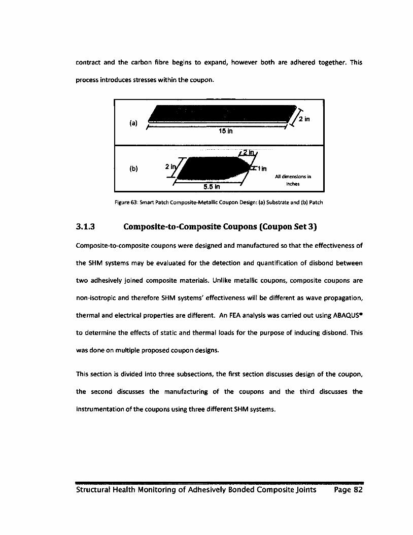
contract and the carbon fibre begins to expand, however both are adhered together. This
process introduces stresses within the coupon.
All dimensions in inches
Figure 63: Smart Patch Composite-Metallic Coupon Design: (a) Substrate and (b) Patch
3.1.3 Composite-to-Composite Coupons (Coupon Set 3)
Composite-to-composite coupons were designed and manufactured so that the effectiveness of
the SHM systems may be evaluated for the detection and quantification of disbond between
two adhesively joined composite materials. Unlike metallic coupons, composite coupons are
non-isotropic and therefore SHM systems' effectiveness will be different as wave propagation,
thermal and electrical properties are different. An FEA analysis was carried out using ABAQUS*
to determine the effects of static and thermal loads for the purpose of inducing disbond. This
was done on multiple proposed coupon designs.
This section is divided into three subsections, the first section discusses design of the coupon,
the second discusses the manufacturing of the coupons and the third discusses the
instrumentation of the coupons using three different SHM systems.
Structural Health Monitoring of Adhesively Bonded Composite Joints Page 82

3.1.3.1 Coupon design requirements
In addition to other evaluation requirements, SHM systems used within this study were tested
for their effectiveness for the detection of disbond between adhesive joints on composite
components. For this reason, the coupons were specially designed with a joint that would fail at
a predefined location with high repeatability. This approach was done to limit the amount of
NDE inspections required to determine and locate failure within the adhesive; this allowed for
quick SHM system evaluation. To meet the overall objective, a series of requirements were
composed to aid in the design of the coupons; these requirements are listed in Table 1.
Table 1: Coupon Design Requirements
Requirement Number
Requirement Name Requirement Text
1. Coupon The designed coupon must contain an adhesive joint that must fail during testing.
2. Material Utilization The designed coupon must be composed of two distinct materials.
2.1. Materials Composition Both materials used within this study must be composite.
2.2. Substrate The substrate must be composed of carbon fibre material.
2.3. Patch The patch must be constructed of a different composite material.
2.4. Adhesive The adhesive must be of consistent thickness.
3. Dimensions The coupon must be designed to fit within a test frame with a maximum grip width of 4 inches.
3.1. Length The coupon must be at least 15 inches in length.
3.2. Width The coupon must be at least 2 inches in width.
4. Loading The coupon must be able to withstand a load without failure other than that of disbond.
4.1. Disbond Loading The patch must disbond from the substrate at a load less than 20,000 lb.
To meet design requirements, three materials were chosen. Materials of choice were based on
availability, cost and mechanical properties. The carbon fibre used for this project was the
CYCOM 5276-1 G40-800 unidirectional prepreg tape. This material was chosen as it is used
Structural Health Monitoring of Adhesively Bonded Composite Joints Page 83
widely throughout multiple projects at National Research Council Canada (NRC) and therefore
was readily available. CYCOM 5276-1 G40-800 prepreg tape material has a modulus of 22.5 Msi,
which will vary depending on layup of the manufactured laminates. Specialty Materials 5521F
unidirectional tape (a boron fibre prepreg) was selected as the material forming the patch that
was bonded to the carbon fibre component. Unlike carbon fibres, boron fibres have a modulus
of 27 Msi. Differences between moduli allowed for a large enough difference in stiffness and
therefore planar stress along the surface of the substrate would be higher than the shear stress
of the adhesive, promoting disbond while statically loaded. Selection of another carbon fibre for
the patch would result in similar moduli and therefore disbond may or may not have initiated.
In addition to its modulus, boron fibre composites were used as repair patch materials for
repairs on aircraft requiring a thermal coefficient that is similar to that of metallic components.
Joining of the carbon fibre and the boron fibre cured components was achieved through the use
of FM73 toughened epoxy film adhesive. FM73 film adhesive is a widely used adhesive within
the aerospace industry as it has excellent mechanical properties for operational temperatures of
aircraft. FM73 also has an imbedded mesh that provides thickness control of the adhesive layer
while temperatures and pressure are applied during the curing process.
In addition to possessing a required combination of mechanical properties, all selected materials
were available at the NRC as they have been used within other ongoing projects.
3.1.3.2 Material properties
Three materials were used for the for the development of the FEA model: CYCOM 5276-1 G40-
800 Tape, Specialty Materials 5521F Tape and CYTEC FM 73 toughened epoxy film as described
in section 3.1.3.1. Property values for all materials were obtained from manufacturer's data
Structural Health Monitoring of Adhesively Bonded Composite Joints Page 84
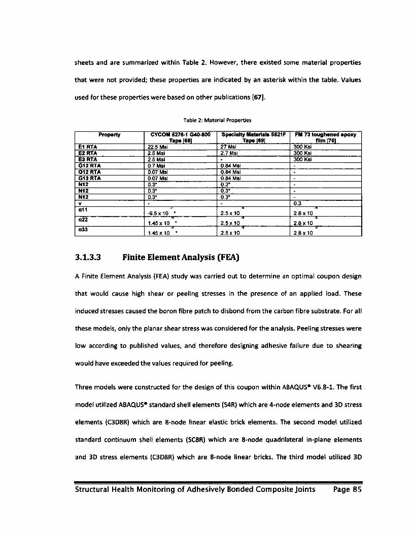
sheets and are summarized within Table 2. However, there existed some material properties
that were not provided; these properties are indicated by an asterisk within the table. Values
used for these properties were based on other publications [67].
Table 2: Material Properties
Property CYCOM 5276-1 G40-800 Tape [681
Specialty Materials 5521F Tape [691
FM 73 toughened epoxy film nroi
E1 RTA 22.5 Msi 27 Msi 300 Ksi E2RTA 2.5 Msi 2.7 Msi 300 Ksi E3RTA 2.5 Msi - 300 Ksi G12 RTA 0.7 Msi 0.84 Msi -
G12 RTA 0.07 Msi 0.84 Msi -
G13 RTA 0.07 Msi 0.84 Msi -
N12 0.3* 0.3* -
N12 0.3* 0.3* -
N12 0.3* 0.3* -
V - - 0.3 o11 •1
-9.5x10 * -©
2.5x10 •9
2.8x10 a22 -9
1 .45x10 * 4
2.5x10 -s
2 .8x10 a33 •9
1.45x10 * <e
2 .5x10 -6
2 .8x10
3.1.3.3 Finite Element Analysis (FEA)
A Finite Element Analysis (FEA) study was carried out to determine an optimal coupon design
that would cause high shear or peeling stresses in the presence of an applied load. These
induced stresses caused the boron fibre patch to disbond from the carbon fibre substrate. For all
these models, only the planar shear stress was considered for the analysis. Peeling stresses were
low according to published values, and therefore designing adhesive failure due to shearing
would have exceeded the values required for peeling.
Three models were constructed for the design of this coupon within ABAQUS* V6.8-1. The first
model utilized ABAQUS* standard shell elements (S4R) which are 4-node elements and 3D stress
elements (C3D8R) which are 8-node linear elastic brick elements. The second model utilized
standard continuum shell elements (SC8R) which are 8-node quadrilateral in-plane elements
and 3D stress elements (C3D8R) which are 8-node linear bricks. The third model utilized 3D
Structural Health Monitoring of Adhesively Bonded Composite Joints Page 85

stress element (C3D20) which is a 20-node quadratic reduced integration bricks and 3D stress
elements (C3D8R) which are 8-node linear bricks, reduced integration. S4R, SC8R and C3D20
elements were used on composite components within each one of their respective models while
C3D8R elements were used only on the adhesive for each of the models. Due to the
computational properties of elements used within each model, each of the models was used for
specific application(s). Conventional shell elements allow for computation of planar stresses and
are not adequate for the analysis of out-of-plane stresses. Also, models utilizing this type of
element were assigned a single element through the thickness of the meshed component. For
these reasons, the first model was used with its inherent approximations to quickly evaluate
parameters such as geometry and composite layup that would be required to induce disbond
within the adhesive joint. Continuum shell elements used within the second model are similar
to conventional shell elements with the exception of through-thickness properties. Through the
use of continuum shell elements, multi-layer composites were modeled to evaluate planar
stresses on each composite ply; this was achieved by assigning a layer of shell elements to each
composite ply. Results of model 2 were compared to those of model 1. The third model utilized
3D stress elements. These elements allowed for the computation of stress and strains in all
directions. Thermal residual stresses which were induced during the bonding process could not
be computed through the use of the previous two models as elements used within those models
allowed for the calculation of only planar stresses while thermal expansion occurs in all three
axes. Through the use of 3D stress elements, model 3 was used to compute thermal residual 3D
stresses.
A mesh dependency analysis was carried out for each of the three models to determine the
minimum amount of elements required to have converged stresses. Multiple analyses were
carried out on each model, each with increasing element count. Stresses for a common node
Structural Health Monitoring of Adhesively Bonded Composite Joints Page 86

found in each analysis were allowed to converge to 10% of the previous two analyses. Figure 64
shows the location of the common node used for each analysis. Figure 65 shows stresses for
model 1 versus the number of elements; each point on this graph corresponds to a different
analysis. It is evident from the graph, that model 1 converges using approximately 50,000
elements. Figure 66 shows stresses for model 2 versus the number of elements. It is evident
from the graph that model 2 converges using approximately 260,000 elements. Figure 67 shows
stresses for model 3 versus the number of elements. Model 3 was found to converge using
170,000 elements.
Figure 64: Common Stress Node
Structural Health Monitoring of Adhesively Bonded Composite Joints Page 87
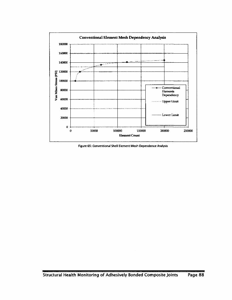
Conventional Element Mesh Dependency Analysis
180000
160000
140000
S-120000 X &
1 100000 (A « .3 80000 2 e > 60000
40000
20000
0
•
/ /
— C o n v e n t i o n a l Elements Dependency
— Upper Limit
—— Lower Limit
I
-
— C o n v e n t i o n a l Elements Dependency
— Upper Limit
—— Lower Limit
I
-
— C o n v e n t i o n a l Elements Dependency
— Upper Limit
—— Lower Limit
I
-
— C o n v e n t i o n a l Elements Dependency
— Upper Limit
—— Lower Limit
I
-
— C o n v e n t i o n a l Elements Dependency
— Upper Limit
—— Lower Limit
I
-
50000 100000 150000
Element Count 200000 250000
Figure 65: Conventional Shell Element Mesh Dependence Analysis
Structural Health Monitoring of Adhesively Bonded Composite Joints Page 88
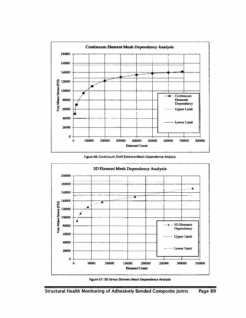
Continuum Element Mesh Dependency Analysis
180000
160000
140000
g" 120000 fin
§ 100000 tA J 80000
e o > 60000
40000
20000
0
r • Continuum Elements Dependency
• Upper Limit
• Lower Limit
0 100000 200000 300000 400000 500000 600000 700000 800000
Element Count
Figure 66: Continuum Shell Element Mesh Dependence Analysis
3D Element Mesh Dependency Analysis
200000
180000
160000
„ 140000
eu T 120000 « S "2 iooooo M S 80000 § > 60000
40000
20000
0
A
.A" A'
A
A A * 3D Elements
Dependency
Upper Limit
Lower Limit
__J 1
* 3D Elements Dependency
Upper Limit
Lower Limit
__J 1
* 3D Elements Dependency
Upper Limit
Lower Limit
__J 1
* 3D Elements Dependency
Upper Limit
Lower Limit
__J 1
* 3D Elements Dependency
Upper Limit
Lower Limit
__J 1 0 50000 100000 150000 200000 250000 300000 350000
Element Count
Figure 67:3D Stress Element Mesh Dependence Analysis
Structural Health Monitoring of Adhesively Bonded Composite Joints Page 89

3.1.3.3.1 Conventional shell model (Model 1)
While designing composite components, there are a few parameters that may be changed in
order to affect performance characteristics of the components, these include: fibre material,
resin material, ply count, ply orientation and geometry. For this model in particular, three
parameters where varied for coupon design optimization: patch shape, patch geometry, and ply
orientation. While testing the effect of each parameter, all other parameters were held
constant. Of all tested parameters, those yielding the highest Von Mises stresses on the
adhesive layer where chosen and then carried through to the next model.
There are several different coupon designs that would have induced disbond within the
adhesive layer under static load; all of which would have been adequate for the primary
objective of this study, but only one was utilized. A starting point for the design of the
composite-to-composite coupons was based on the composite-to-metallic design described in
section 3.1.2. The exact dimensions and geometry of coupons described in section 3.1.2 were
duplicated for an initial design within ABAQUS and is shown in Figure 68.
All dimensions in inches fcarfrQn pj^
IBoron Fibre
N) o o
Figure 68: Smart Patch Phase 1 & 2 Coupon Design (measurements in inches)
Structural Health Monitoring of Adhesively Bonded Composite Joints Page 90
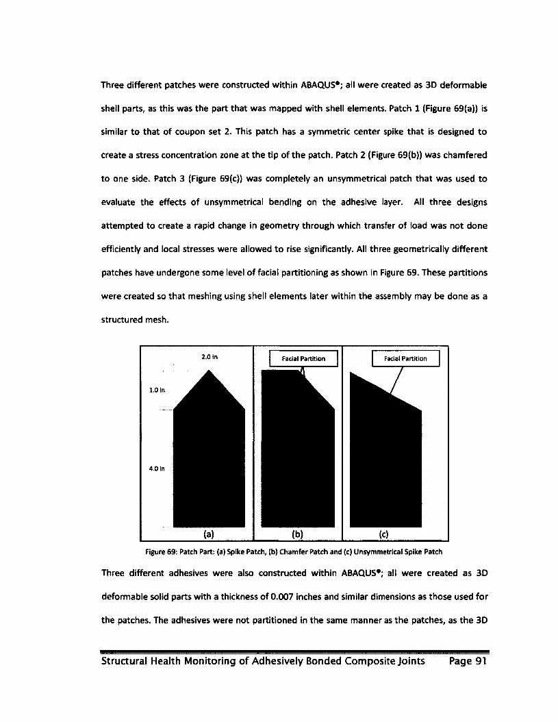
Three different patches were constructed within ABAQUS*; all were created as 3D deformable
shell parts, as this was the part that was mapped with shell elements. Patch 1 (Figure 69(a)) is
similar to that of coupon set 2. This patch has a symmetric center spike that is designed to
create a stress concentration zone at the tip of the patch. Patch 2 (Figure 69(b)) was chamfered
to one side. Patch 3 (Figure 69(c)) was completely an unsymmetrical patch that was used to
evaluate the effects of unsymmetrical bending on the adhesive layer. All three designs
attempted to create a rapid change in geometry through which transfer of load was not done
efficiently and local stresses were allowed to rise significantly. All three geometrically different
patches have undergone some level of facial partitioning as shown in Figure 69. These partitions
were created so that meshing using shell elements later within the assembly may be done as a
structured mesh.
Facial Partition Facial Partition
Figure 69: Patch Part: (a) Spike Patch, (b) Chamfer Patch and (c) Unsymmetrical Spike Patch
Three different adhesives were also constructed within ABAQUS*; all were created as 3D
deformable solid parts with a thickness of 0.007 inches and similar dimensions as those used for
the patches. The adhesives were not partitioned in the same manner as the patches, as the 3D
Structural Health Monitoring of Adhesively Bonded Composite Joints Page 91
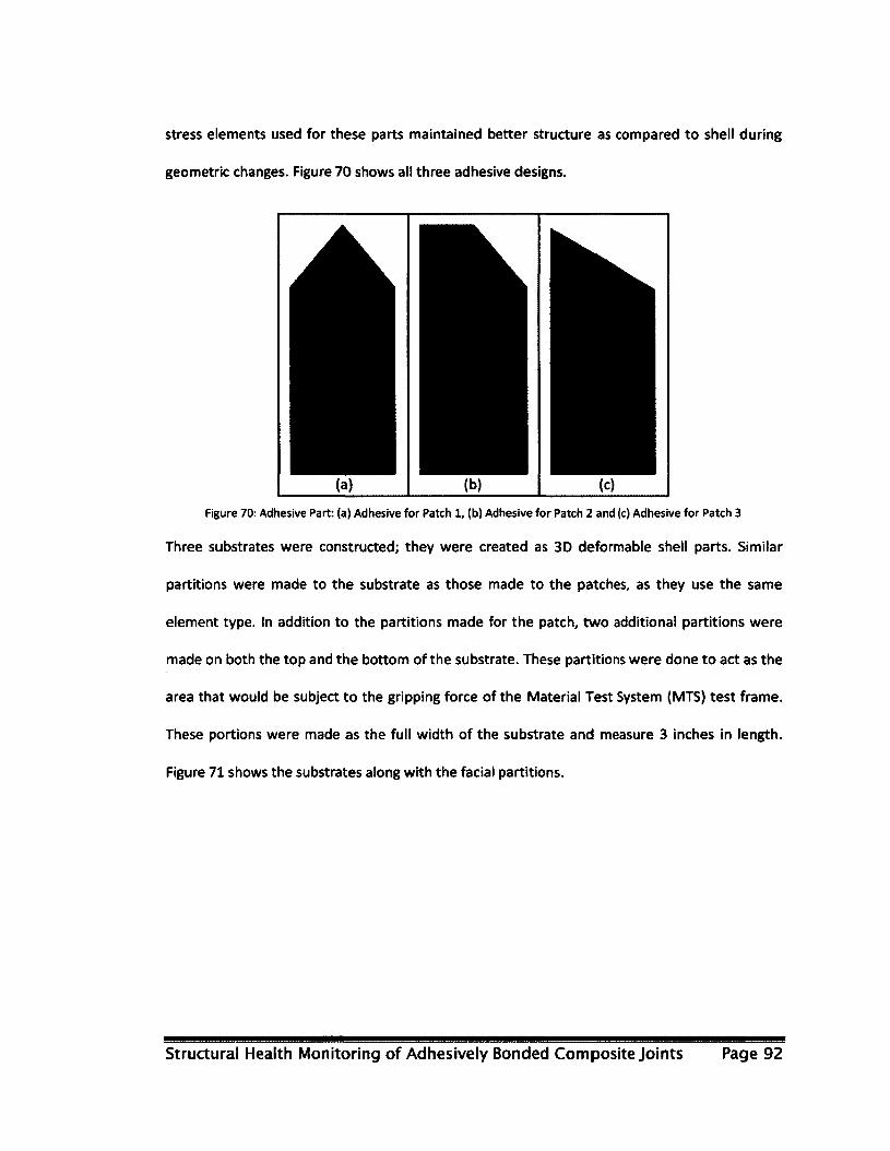
stress elements used for these parts maintained better structure as compared to shell during
geometric changes. Figure 70 shows all three adhesive designs.
Figure 70: Adhesive Part: (a) Adhesive for Patch 1, (b) Adhesive for Patch 2 and (c) Adhesive for Patch 3
Three substrates were constructed; they were created as 3D deformable shell parts. Similar
partitions were made to the substrate as those made to the patches, as they use the same
element type. In addition to the partitions made for the patch, two additional partitions were
made on both the top and the bottom of the substrate. These partitions were done to act as the
area that would be subject to the gripping force of the Material Test System (MTS) test frame.
These portions were made as the full width of the substrate and measure 3 inches in length.
Figure 71 shows the substrates along with the facial partitions.
Structural Health Monitoring of Adhesively Bonded Composite Joints Page 92
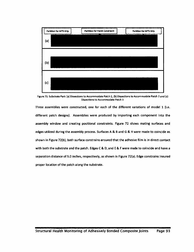
Partition for Patch Constraint Partition for MTS Grip
Figure 71: Substrate Part: (a) Dissections to Accommodate Patch 1, (b) Dissections to Accommodate Patch 2 and (c) Dissections to Accommodate Patch 3
Three assemblies were constructed, one for each of the different variations of model 1 (i.e.
different patch designs). Assemblies were produced by importing each component into the
assembly window and creating positional constraints. Figure 72 shows mating surfaces and
edges utilized during the assembly process. Surfaces A & B and G & H were made to coincide as
shown in Figure 72(b), both surface constrains ensured that the adhesive film is in direct contact
with both the substrate and the patch. Edges C & D, and E & F were made to coincide and have a
separation distance of 5.0 inches, respectively, as shown in Figure 72(a). Edge constrains insured
proper location of the patch along the substrate.
Structural Health Monitoring of Adhesively Bonded Composite Joints Page 93

Edges
F, K
E, I
Patch | . | Surfaces A
in 1
V
Adhesive
Substrate
(b)
Figure 72: Assembly Position Constraints: (a) Isotropic View and (b) Side, Exploded View
In addition to position constraints, tie constraints were introduced into the model. Tie
constraints were utilized to join nodes found on surface A with nodes on B and nodes on H with
nodes on G. Through this tie constraint, boundary conditions were shared between two
adjacent surfaces and ultimately identical displacements.
Partitions shown in Figure 71 measuring 2.0 x 3.0 inches were subjected to both the load and
boundary condition as shown in Figure 73. These sections were created to simulate the grips
which were used for load application. The applied load was created as a traction load and was
applied to both sides of the substrate (front and back). The traction load was created with a
uniform distribution. The boundary condition was set on the bottom section of the coupon
(front and back); this boundary condition was created such that it did not allow motion along
any of the three axes.
Structural Health Monitoring of Adhesively Bonded Composite Joints Page 94
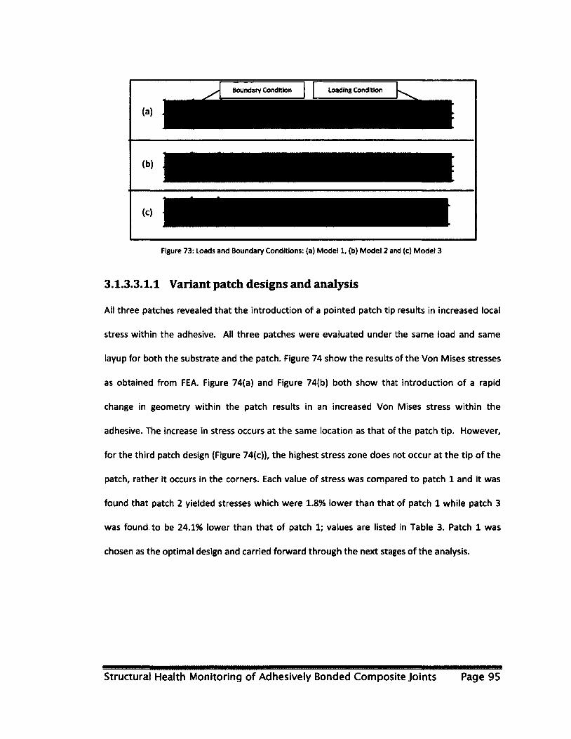
Boundary Condition Loading Condition
Figure 73: Loads and Boundary Conditions: (a) Model 1, (b) Model 2 and (c) Model 3
3.1.3.3.1.1 Variant patch designs and analysis
All three patches revealed that the introduction of a pointed patch tip results in increased local
stress within the adhesive. All three patches were evaluated under the same load and same
layup for both the substrate and the patch. Figure 74 show the results of the Von Mises stresses
as obtained from FEA. Figure 74(a) and Figure 74(b) both show that introduction of a rapid
change in geometry within the patch results in an increased Von Mises stress within the
adhesive. The increase in stress occurs at the same location as that of the patch tip. However,
for the third patch design (Figure 74(c)), the highest stress zone does not occur at the tip of the
patch, rather it occurs in the corners. Each value of stress was compared to patch 1 and it was
found that patch 2 yielded stresses which were 1.8% lower than that of patch 1 while patch 3
was found to be 24.1% lower than that of patch 1; values are listed in Table 3. Patch 1 was
chosen as the optimal design and carried forward through the next stages of the analysis.
Structural Health Monitoring of Adhesively Bonded Composite Joints Page 95
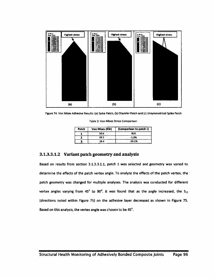
Highest stress Highest stress Highest stress
Figure 74: Von Mises Adhesive Results: (a) Spike Patch, (b) Chamfer Patch and (c) Unsymmetrical Spike Patch
Table 3: Von Mises Stress Comparison
Patch Von Mises (KSI) (Comparison to patch 1)
1 50.6 N/A
2 49.1 -1.8%
3 38.4 -24.1%
3.1.3.3.1.2 Variant patch geometry and analysis
Based on results from section 3.1.3.3.1.1, patch 1 was selected and geometry was varied to
determine the effects of the patch vertex angle. To analyze the effects of the patch vertex, the
patch geometry was changed for multiple analyses. The analysis was conducted for different
vertex angles varying from 45° to 90°. It was found that as the angle increased, the Si2
(directions noted within Figure 75) on the adhesive layer decreased as shown in Figure 75.
Based on this analysis, the vertex angle was chosen to be 45°.
Structural Health Monitoring of Adhesively Bonded Composite Joints Page 96
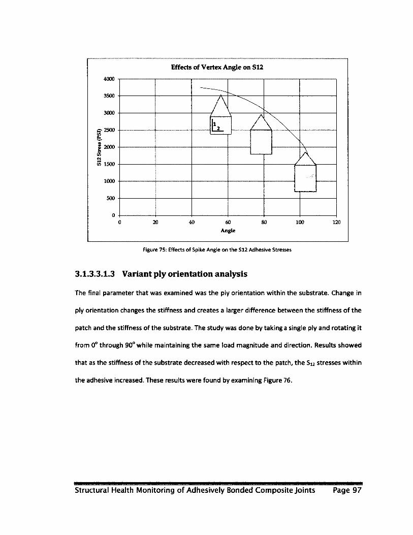
Effects of Vertex Angle on S12
4000
3500
3000
a- 2500
2000
N & 1500
1000
500
0 0 20 40 60 80 100 120
Angle
Figure 75: Effects of Spike Angle on the S12 Adhesive Stresses
3.1.3.3.1.3 Variant ply orientation analysis
The final parameter that was examined was the ply orientation within the substrate. Change in
ply orientation changes the stiffness and creates a larger difference between the stiffness of the
patch and the stiffness of the substrate. The study was done by taking a single ply and rotating it
from 0° through 90° while maintaining the same load magnitude and direction. Results showed
that as the stiffness of the substrate decreased with respect to the patch, the Si2 stresses within
the adhesive increased. These results were found by examining Figure 76.
Structural Health Monitoring of Adhesively Bonded Composite Joints Page 97

Effects of Ply Orientation on S12
Fiber
direction
400
200
o 4 0 10 20 30 40 50 60 70 80 90 100
Angle
Figure 76: Effects of Ply Angle on S12
3.1.3.3.1.4 Summary of results
FEA results using the simplified conventional shell elements revealed that a symmetric patch
with a vertex forming 45° yields the highest Si2 stress within the adhesive layer. Also, the greater
the difference of stiffness between the patch and the substrate the greater stress build up
within the adhesive layer.
Using these results, the substrate layup was chosen to be of only ± 45° and was set to [45, -45,
45, -45]s; this was chosen because it yields the lowest stiffness along the loading direction as
well as ensuring that the substrate can support the applied load without failure by matrix
shearing. The patch layup was chosen to be made of primarily 0° and was set to [0, 0, 45, -45]s.
The 0° yields greatest stiffness along the loading direction. The introduction of ± 45° was done
so that the patch has some strength perpendicular to the applied load.
Structural Health Monitoring of Adhesively Bonded Composite Joints Page 98

3.1.3.3.2 Continuum shell model (Model 2)
The continuum shell model was the second model that was developed for analysis of the
coupon design. Due to the continuum shell element properties, this model was only used to
determine individual ply stresses. These stresses were then compared to the results of the
conventional model to determine the model's efficiency and accuracy.
The continuum model is very similar to the conventional model in its setup; however, there are
small differences that have been carried out in order to accommodate the continuum shell
element meshing. This section only discusses differences between both models and compares
their results.
Both the patch and substrate were constructed within ABAQUS® as 3D deformable solid parts
within the continuum shell model. 3D deformable solids allow for through thickness assignment
of elements as opposed to shell parts which were used in conjunction with the conventional
shell elements. The constructed patch was that of Type 1. Remainder patch designs were
discarded as they resulted in lower shear stresses in the presence of the same applied load.
Implementation of the continuum elements (SC8R) was done by defining a sweep mesh. A
sweeping mesh is the application of elements in layers; this was done to layer multiple planar
element sheets through the thickness of the component. The layering of planar element sheets
was done through the thickness of the component as shown in Figure 77, which had a
predefined 8 nodal count along the edges (1 node for each ply). This sweep was done for both
the substrate and the patch. By stacking 8 layers of elements, stresses along the x-y coordinates
were evaluated for each individual ply.
Structural Health Monitoring of Adhesively Bonded Composite joints Page 99
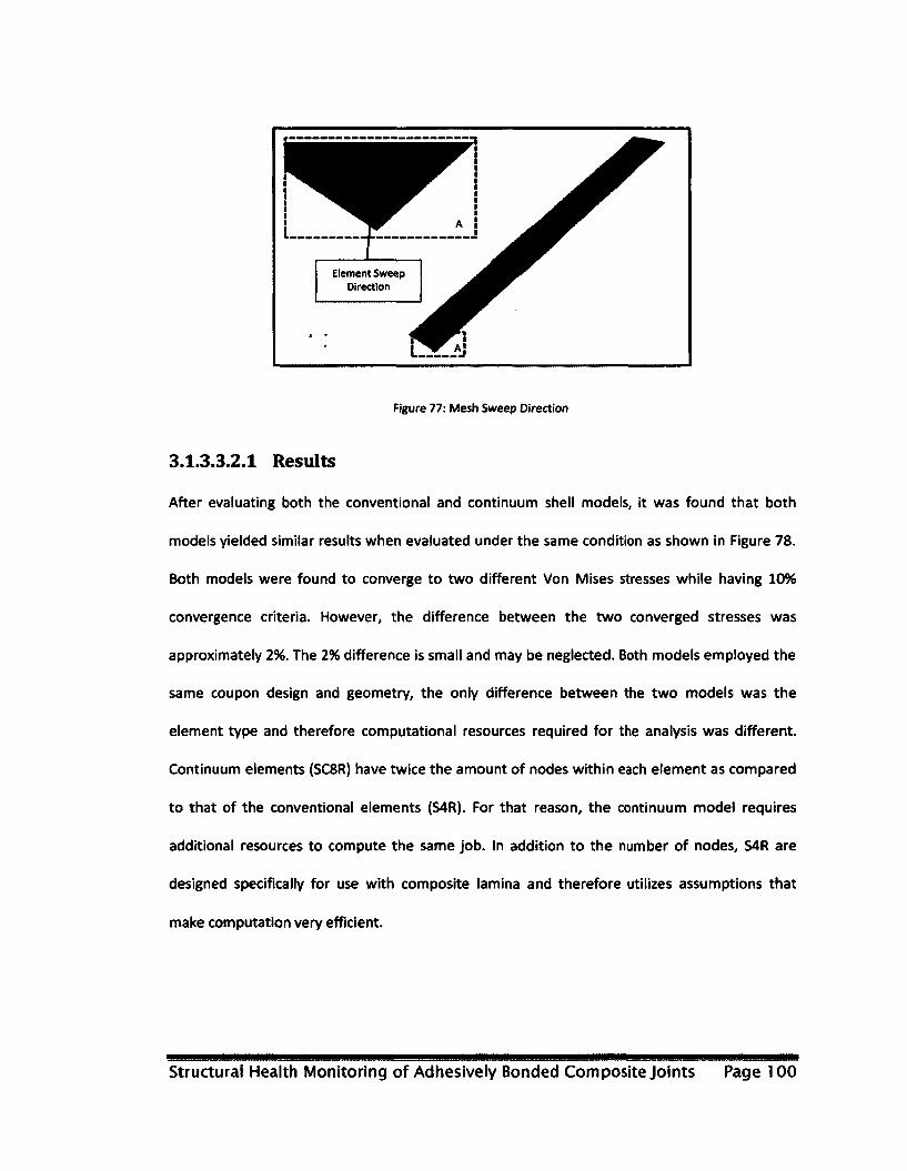
Element Sweep Direction
Figure 77: Mesh Sweep Direction
3.1.3.3.2.1 Results
After evaluating both the conventional and continuum shell models, it was found that both
models yielded similar results when evaluated under the same condition as shown in Figure 78.
Both models were found to converge to two different Von Mises stresses while having 10%
convergence criteria. However, the difference between the two converged stresses was
approximately 2%. The 2% difference is small and may be neglected. Both models employed the
same coupon design and geometry, the only difference between the two models was the
element type and therefore computational resources required for the analysis was different.
Continuum elements (SC8R) have twice the amount of nodes within each element as compared
to that of the conventional elements (S4R). For that reason, the continuum model requires
additional resources to compute the same job. In addition to the number of nodes, S4R are
designed specifically for use with composite lamina and therefore utilizes assumptions that
make computation very efficient.
Structural Health Monitoring of Adhesively Bonded Composite Joints Page 100
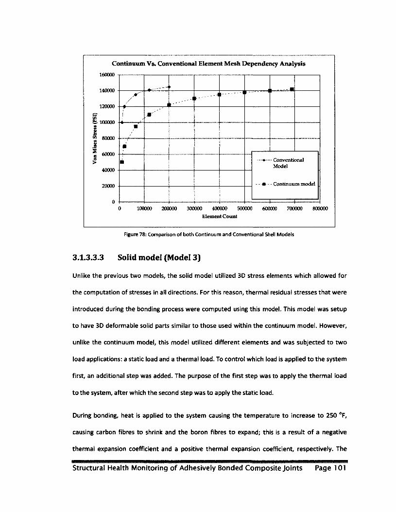
Continuum Vs. Conventional Element Mesh Dependency Analysis
160000
c £
140000
120000
100000
1 w 80000 m M
g 60000 o >
40000
20000
0
/ /
i . . I
y - ' ~
- - 4 y -
i ' r-
T
m
m
• —•— Conventional Model
- - » - - Continuum model
1 r—1
—•— Conventional Model
- - » - - Continuum model
1 r—1
—•— Conventional Model
- - » - - Continuum model
1 r—1
100000 200000 300000 400000 500000 600000 700000 800000
Element Count
Figure 78: Comparison of both Continuum and Conventional Shell Models
3.1.3.3.3 Solid model (Model 3)
Unlike the previous two models, the solid model utilized 3D stress elements which allowed for
the computation of stresses in all directions. For this reason, thermal residual stresses that were
introduced during the bonding process were computed using this model. This model was setup
to have 3D deformable solid parts similar to those used within the continuum model. However,
unlike the continuum model, this model utilized different elements and was subjected to two
load applications: a static load and a thermal load. To control which load is applied to the system
first, an additional step was added. The purpose of the first step was to apply the thermal load
to the system, after which the second step was to apply the static load.
During bonding, heat is applied to the system causing the temperature to increase to 250 °F,
causing carbon fibres to shrink and the boron fibres to expand; this is a result of a negative
thermal expansion coefficient and a positive thermal expansion coefficient, respectively. The
Structural Health Monitoring of Adhesively Bonded Composite Joints Page 101

FM73 adhesive cures at 250 °F and once the system is allowed to cool, the coupon will not
return to its original state and therefore thermal residual stresses are developed within the
system. Simulation of this within FEA was done through the creation of a boundary condition
which set the entire model at an equilibrium temperature of 250 °F; in addition to this boundary
condition, a second boundary condition was created within a second step. This second boundary
condition imposes an equilibrium temperature of 74 °F. By creating these two boundary
conditions, ABAQUS* is able to calculate the displacements of each node due to temperature
change. For this problem, only the steady state result was of interest; therefore imposing an
initial and final temperature is adequate for this problem as calculated displacements due to
expansion and contraction were used to calculate stresses.
3.1.3.3.3.1 Results
Figure 79 shows stress distribution in the x-y plane for all components after application of both
thermal and static loads. Stress distribution shows that the rapid change in geometry (i.e. patch
vertex) affects the stresses locally as expected. The applied force region in Figure 79 shows a
gradient of stress; in real life this would not occur as the area in the grip would not be permitted
to deform. A similar stress distribution does not occur in the applied boundary condition region
because nodes are not permitted to strain within all directions. A boundary condition imposing
relative location of nodes to neighbouring nodes in the applied load region was not imposed as
stress and strain distribution at the loading area had no impact on the area of interest. Figure 80
shows stress distribution within the x-y plane for both the patch and the adhesive. Both the
patch and adhesive stress distributions appear to be mirrored along the center line of the
coupon, with a positive stress side and a negative stress side; both equal in magnitude. This
symmetry in distribution is due to both the layup of the substrate and the patch. Through the
Structural Health Monitoring of Adhesively Bonded Composite Joints Page 102

use of a substrate with a [45, -45, 45, -45]s and a patch with a [0, 0, 45, -45]s layup stresses are
not expected to be highest at the vertex, rather at the area of the highest stiffness. The area of
highest stiffness occurs at the 45° angle and therefore the stresses at 90° separation occur in the
opposite magnitude as the ply is weakest in that direction.
Structural Health Monitoring of Adhesively Bonded Composite Joints Page 103
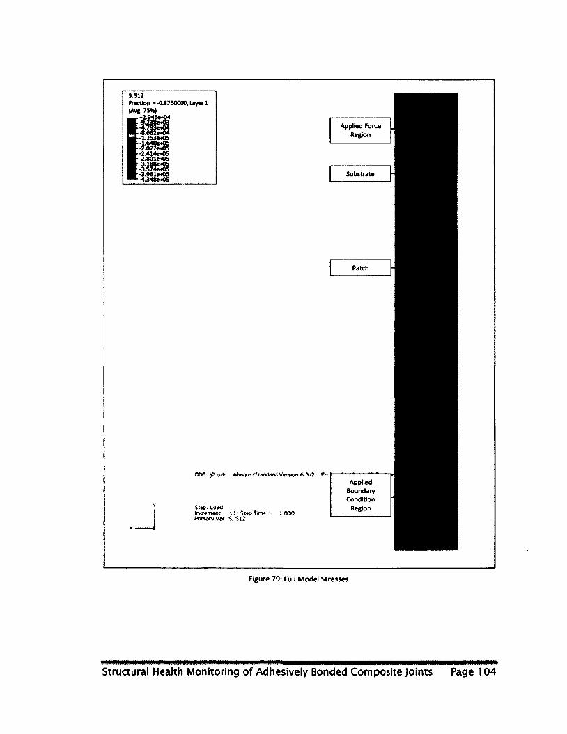
S.S12 Fraction »-0.8750000. Layer 1 (Avg: 75*)
r+2.945et04 t-9J38e«03 h-4-793e404 "8.662e404 ,-1.253e*05 f--1.640e+05 r-2.027e*05 ^ -2.414€+05 -2.801e*05 -3.18a«*05 h -3.574«+05 r -3.961e+05
-4.348e+05
Applied Force Region
Substrate
Patch
OCXS- fi !>•*> V>n«5« 6 0-? Fn
Sup: \.omi t 1 $»p
Primary Vor $, -Jti tooo
Applied Boundary Condition
Region
Figure 79: Full Model Stresses
Structural Health Monitoring of Adhesively Bonded Composite Joints Page 104
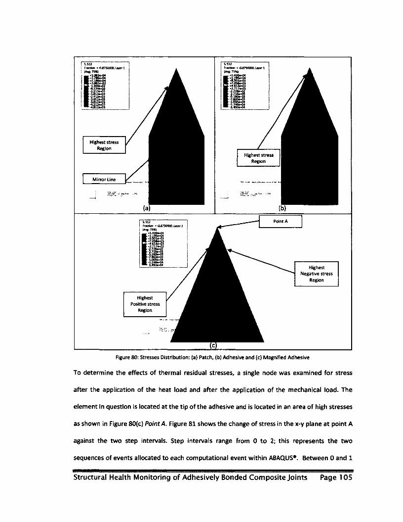
S, &12 Fraction -04750000. Uyerl (AMf;7S*J
+23£5*«04 , *l!7M*«04 k •1.186*04 -•5A61e*C3 »-1.369**02 k -6.134^03 f-JL213«*03 r-LS139*03 --2.413a«03 •i012*«03 . 1612**03 h-4iU*<03 ••-4J12«*03
Highest stress Region
Mirror Line
S,512 Fraction - -04750000, L^ef 1 (Avt:75%)
+1A39-04
«7.058*MK *4.6146*03 •2.7l7»*03 2.72Be*02 .716»*3
1.249e*04 1.493*«04
Highest stress Region
) fraction --OJ75CCOO, Ltyer 2 ! {Av»: 75H)
r *1.439*404 L+1.195**04 t«930U«03 L«7.05S^03 f *4.614e*03 f+2.717e*03 -•2.728e*02 ,--2.7l6e«03 h-5^60*03 ••7.6fl3®*03
Point A
Highest Positive stress
Region
Highest Negative stress
Region
Figure 80: Stresses Distribution: (a) Patch, (b) Adhesive and (c) Magnified Adhesive
To determine the effects of thermal residual stresses, a single node was examined for stress
after the application of the heat load and after the application of the mechanical load. The
element in question is located at the tip of the adhesive and is located in an area of high stresses
as shown in Figure 80(c) Point A. Figure 81 shows the change of stress in the x-y plane at point A
against the two step intervals. Step intervals range from 0 to 2; this represents the two
sequences of events allocated to each computational event within ABAQUS*. Between 0 and 1
Structural Health Monitoring of Adhesively Bonded Composite Joints Page 105
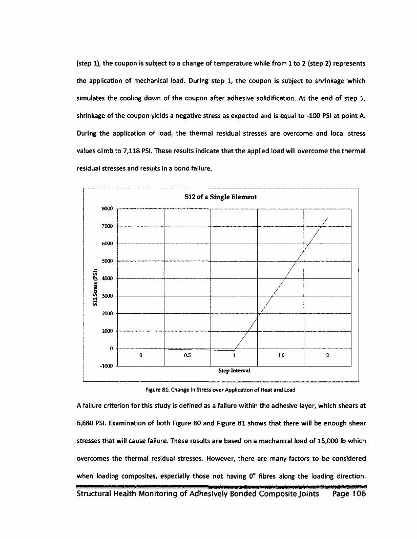
(step 1), the coupon is subject to a change of temperature while from 1 to 2 (step 2) represents
the application of mechanical load. During step 1, the coupon is subject to shrinkage which
simulates the cooling down of the coupon after adhesive solidification. At the end of step 1,
shrinkage of the coupon yields a negative stress as expected and is equal to -100 PSI at point A.
During the application of load, the thermal residual stresses are overcome and local stress
values climb to 7,118 PSI. These results indicate that the applied load will overcome the thermal
residual stresses and results in a bond failure.
S12 of a Single Element
Step Interval
Figure 81: Change in Stress over Application of Heat and Load
A failure criterion for this study is defined as a failure within the adhesive layer, which shears at
6,680 PSI. Examination of both Figure 80 and Figure 81 shows that there will be enough shear
stresses that will cause failure. These results are based on a mechanical load of 15,000 lb which
overcomes the thermal residual stresses. However, there are many factors to be considered
when loading composites, especially those not having 0° fibres along the loading direction.
Structural Health Monitoring of Adhesively Bonded Composite Joints Page 106
Composites having non-zero degree fibres experience failure modes other than fibre breakage
and therefore the strength of the component is not as high as expected. For this reason, the
coupon was later loaded incrementally to determine its ultimate strength. In addition to the
strength of the coupon, SHM instrumentation played an important role for this study as sensors
must withstand the strains for data acquisition. Sample coupons were tested to determine the
coupon ultimate strength as well as sensor adhesion strength. These loads determined the exact
test matrix for all coupons that were manufactured for this project which is described later in
the testing chapter, Chapter 4.
3.1.3.4 Carbon fibre substrate manufacturing
The manufacturing procedure used for the substrates involved accurate ply cutting of CYCOM
5276-1 G40-800 at appropriate angles, stacking plies at the correct orientation, placing the layup
under vacuum and finally curing the layup. All of these steps within the procedure are described
in greater detail within the following subsections.
3.1.3.4.1 CYCOM 5276-1G40-800 prepreg tape cutting
FEA computational analysis revealed that disbond between adhesively bonded components will
occur as a result of sufficient stress build-up within the adhesive layer. Substrate strength for
this study was achieved by two methods: the material property and the component layup. For
this substrate, the optimum layup was found through FEA analysis to be [45, -45, 45, -45]s.
Deviations from those angles will result in either a higher or lower stiffness; this will affect the
material strain in the presence of an applied load. For that reason, it was very important to
maintain ply orientation. Cutting plies and stacking them within ± 2° was difficult for small
coupons as fibres are subject to skewing during handling. To minimize fibre skewing, handling of
Structural Health Monitoring of Adhesively Bonded Composite Joints Page 107
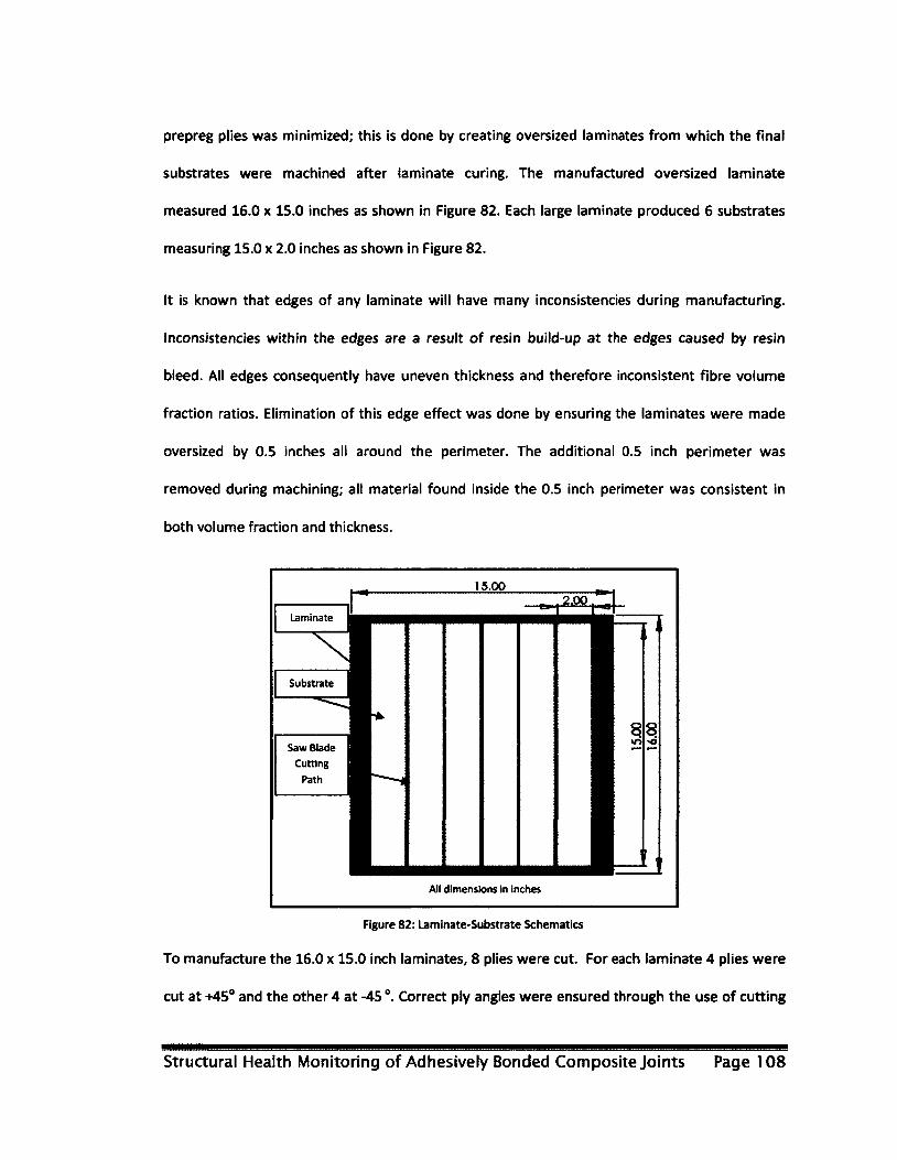
prepreg plies was minimized; this is done by creating oversized laminates from which the final
substrates were machined after laminate curing. The manufactured oversized laminate
measured 16.0 x 15.0 inches as shown in Figure 82. Each large laminate produced 6 substrates
measuring 15.0 x 2.0 inches as shown in Figure 82.
It is known that edges of any laminate will have many inconsistencies during manufacturing.
Inconsistencies within the edges are a result of resin build-up at the edges caused by resin
bleed. All edges consequently have uneven thickness and therefore inconsistent fibre volume
fraction ratios. Elimination of this edge effect was done by ensuring the laminates were made
oversized by 0.5 inches all around the perimeter. The additional 0.5 inch perimeter was
removed during machining; all material found inside the 0.5 inch perimeter was consistent in
both volume fraction and thickness.
Laminate
Substrate
Saw Blade
Cutting
Path
All dimensions in inches
Figure 82: Laminate-Substrate Schematics
To manufacture the 16.0 x 15.0 inch laminates, 8 plies were cut. For each laminate 4 plies were
cut at +45° and the other 4 at -45 °. Correct ply angles were ensured through the use of cutting
Structural Health Monitoring of Adhesively Bonded Composite Joints Page 108
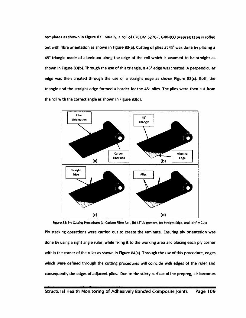
templates as shown in Figure 83. Initially, a roll of CYCOM 5276-1G40-800 prepreg tape is rolled
out with fibre orientation as shown in Figure 83(a). Cutting of plies at 45° was done by placing a
45° triangle made of aluminum along the edge of the roll which is assumed to be straight as
shown in Figure 83(b). Through the use of this triangle, a 45° edge was created. A perpendicular
edge was then created through the use of a straight edge as shown Figure 83(c). Both the
triangle and the straight edge formed a border for the 45° plies. The plies were then cut from
the roll with the correct angle as shown in Figure 83(d).
Fiber
Orientation Triangle
Carbon
Fiber Roll
Aligning
Edge
Straight
Edge
Figure 83: Ply Cutting Procedure: (a) Carbon Fibre Roll, (b) 45° Alignment, (c) Straight Edge, and (d) Ply Cuts
Ply stacking operations were carried out to create the laminate. Ensuring ply orientation was
done by using a right angle ruler, while fixing it to the working area and placing each ply corner
within the corner of the ruler as shown in Figure 84(a). Through the use of this procedure, edges
which were defined through the cutting procedures will coincide with edges of the ruler and
consequently the edges of adjacent plies. Due to the sticky surface of the prepreg, air becomes
Structural Health Monitoring of Adhesively Bonded Composite Joints Page 109
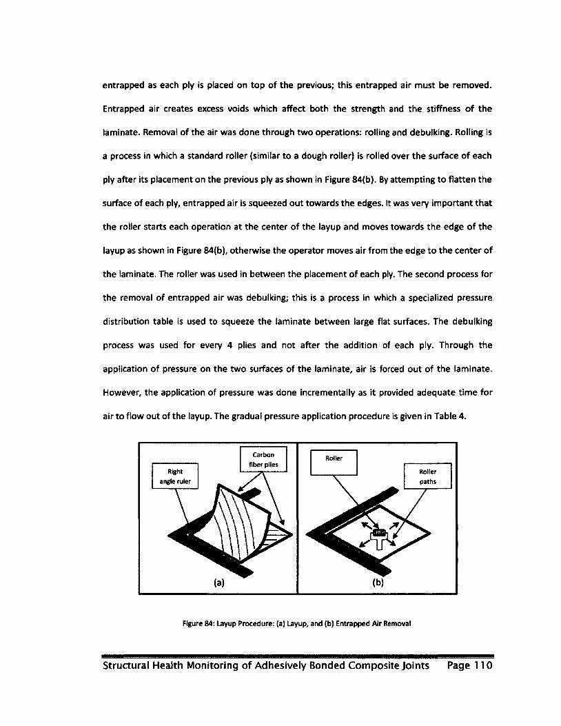
entrapped as each ply is placed on top of the previous; this entrapped air must be removed.
Entrapped air creates excess voids which affect both the strength and the stiffness of the
laminate. Removal of the air was done through two operations: rolling and debulking. Rolling is
a process in which a standard roller (similar to a dough roller) is rolled over the surface of each
ply after its placement on the previous ply as shown in Figure 84(b). By attempting to flatten the
surface of each ply, entrapped air is squeezed out towards the edges. It was very important that
the roller starts each operation at the center of the layup and moves towards the edge of the
layup as shown in Figure 84(b), otherwise the operator moves air from the edge to the center of
the laminate. The roller was used in between the placement of each ply. The second process for
the removal of entrapped air was debulking; this is a process in which a specialized pressure
distribution table is used to squeeze the laminate between large flat surfaces. The debulking
process was used for every 4 plies and not after the addition of each ply. Through the
application of pressure on the two surfaces of the laminate, air is forced out of the laminate.
However, the application of pressure was done incrementally as it provided adequate time for
air to flow out of the layup. The gradual pressure application procedure is given in Table 4.
Carbon
fiber plies Roller
Right
angle ruler
Roller
paths
Figure 84: Layup Procedure: (a) Layup, and (b) Entrapped Air Removal
Structural Health Monitoring of Adhesively Bonded Composite Joints Page 110

Table 4: Debulking Procedure
Vacuum Pressure Time 5PSI 5 minutes 10PSI 5 minutes 15PSI 5 minutes 20PSI 5 minutes 25PSI 5 minutes or more
3.1.3.4.2 Laminate bagging
Laminate bagging is the step in the manufacturing process in which the uncured laminate is
sandwiched between two large aluminum plates (a tool plate and a caul plate) and placed within
a vacuum bag. This was done to prepare the laminate for the autoclave oven; which applied
both heat and pressure for laminate curing. Proper bagging was crucial as it defined the
laminate surface quality, mechanical properties and volume fraction.
The laminate was placed on a large aluminum tool plate as shown in Figure 85(a). The tool plate
was 0.5 inches thick and was used to create a flat surface which the laminate is allowed to
conform to. Teflon film was placed on the tool plate to create a separation medium to ensure
that the laminate does not adhere to the tool plate as shown in Figure 85(a). In addition to the
Teflon, shims were placed all around the perimeter of the laminate and a thermocouple sensor
was placed 0.5 inches away from the laminate as shown in Figure 85(a). Shims measuring 0.04
inches were placed all around the laminate so that thickness and volume fraction of the
laminate may be controlled. Shims supported the weight of a large aluminum caul plate (which
is wrapped in Teflon) which was placed on top of the laminate as shown in Figure 85(a) and
Figure 85(b). The shims created a gap between the tool plate and the caul plate so that the final
thickness of the laminate did not exceed that of the shims. Shim thickness of 0.04 inches
corresponded to 0.005 inches/cured ply as recommended by the manufacturer. Thermocouple
sensors were used to monitor the temperature of the laminate during the cure cycle. A layer of
Structural Health Monitoring of Adhesively Bonded Composite Joints Page 111

porous Teflon was placed on top of the caul plate and tool plate as shown in Figure 85(b).
Porous Teflon was used to limit excess resin bleed from adhesion to surrounding surfaces. In
addition to limiting adhesion, porous Teflon was used as it did not hinder air flow that was
caused by vacuum force. A layer of 0.25 inch breather cloth was added on top of all components
and sealant tape was placed all around the perimeter of the tool plate as shown in Figure 85(c).
Breather cloth acted as a separating medium between the vacuum bag and all other
components; allowing air flow while vacuum is applied. A vacuum bag was placed and an air
tight seal was created with the sealant tape all around the perimeter of the tool plate. A
pressure valve was placed by creating a small incision in the bag as shown in Figure 85(d). The
packaged laminate was kept under 30 PSI of pressure by attaching a pump to the mushroom
valve until placed into the autoclave oven where the curing process was carried out and
pressure within the autoclave oven reached that of 85 PSI.
Structural Health Monitoring of Adhesively Bonded Composite Joints Page 112
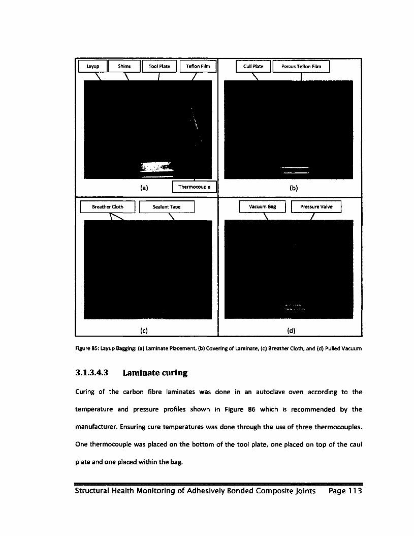
Shims Teflon Rim Cull Plate Porous Teflon Film
Thermocouple
Breather Cloth Vacuum Bag Pressure Valve Sealant Tape
Figure 85: Layup Bagging: (a) Laminate Placement, (b) Covering of Laminate, (c) Breather Cloth, and (d) Pulled Vacuum
3.1.3.4.3 Laminate curing
Curing of the carbon fibre laminates was done in an autoclave oven according to the
temperature and pressure profiles shown in Figure 86 which is recommended by the
manufacturer. Ensuring cure temperatures was done through the use of three thermocouples.
One thermocouple was placed on the bottom of the tool plate, one placed on top of the caul
plate and one placed within the bag.
Structural Health Monitoring of Adhesively Bonded Composite Joints Page 11 3
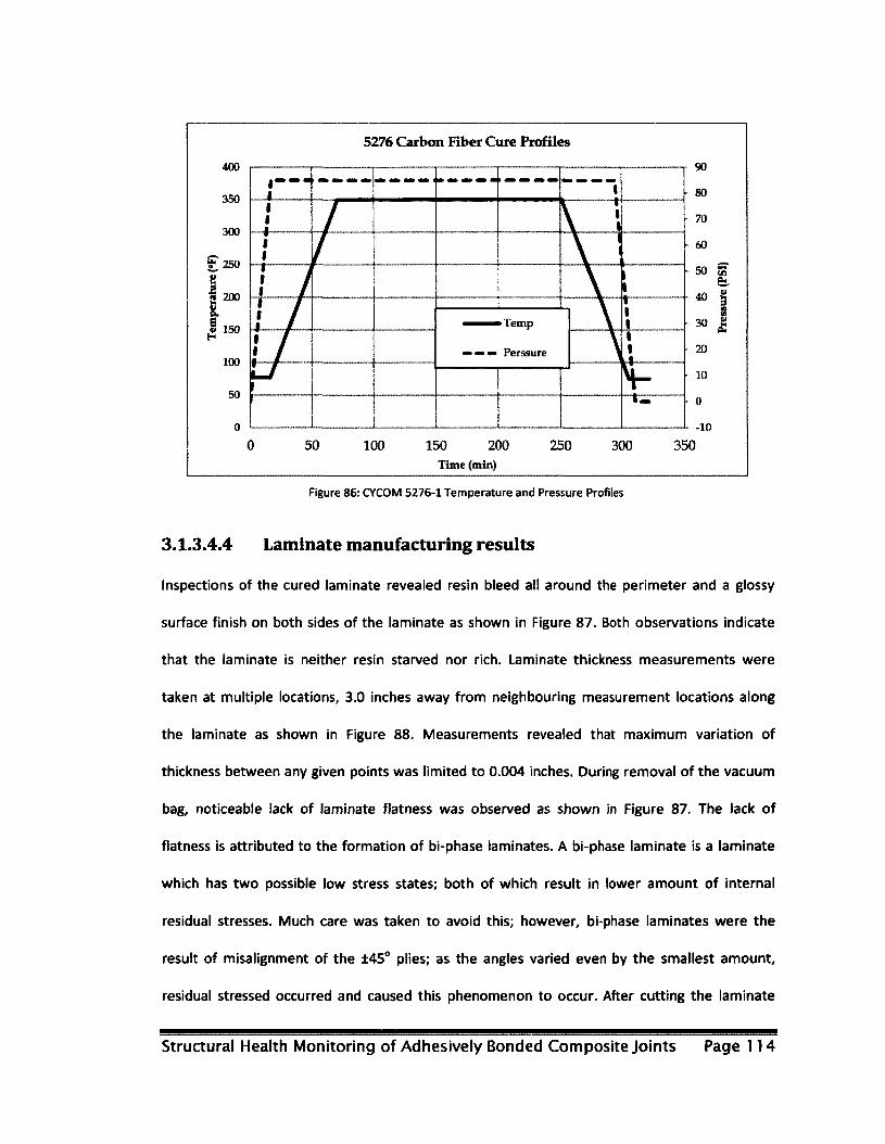
5276 Carbon Fiber Cure Profiles
Time (min)
Figure 86: CYCOM 5276-1 Temperature and Pressure Profiles
3.1.3.4.4 Laminate manufacturing results
Inspections of the cured laminate revealed resin bleed all around the perimeter and a glossy
surface finish on both sides of the laminate as shown in Figure 87. Both observations indicate
that the laminate is neither resin starved nor rich. Laminate thickness measurements were
taken at multiple locations, 3.0 inches away from neighbouring measurement locations along
the laminate as shown in Figure 88. Measurements revealed that maximum variation of
thickness between any given points was limited to 0.004 inches. During removal of the vacuum
bag, noticeable lack of laminate flatness was observed as shown in Figure 87. The lack of
flatness is attributed to the formation of bi-phase laminates. A bi-phase laminate is a laminate
which has two possible low stress states; both of which result in lower amount of internal
residual stresses. Much care was taken to avoid this; however, bi-phase laminates were the
result of misalignment of the 145° plies; as the angles varied even by the smallest amount,
residual stressed occurred and caused this phenomenon to occur. After cutting the laminate
Structural Health Monitoring of Adhesively Bonded Composite Joints Page 114
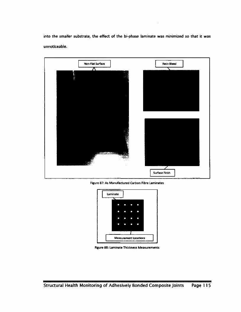
into the smaller substrate, the effect of the bi-phase laminate was minimized so that it was
unnoticeable.
Non-Flat Surface Resin Bleed
Surface Finish
Figure 87: As Manufactured Carbon Fibre Laminates
Laminate
Measurement Locations
Figure 88: Laminate Thickness Measurements
Structural Health Monitoring of Adhesively Bonded Composite joints Page 11 5

3.1.3.5 Patch manufacturing
The manufacturing procedure used for the patches is very similar to that which was used for
manufacturing of the substrates. However, unlike the substrate, the patches had a different
layup: [0,0,45, -45]s.
The Specialty Materials 5521F boron prepreg tape is only 6.0 inches wide and therefore cutting
plies that are at ± 45° did not achieve large enough laminates that could produce two or more
patches. Instead of large laminates, laminates measuring 5.5 x 2.5 inches were created following
the same procedure as in section 3.1.3.4.1. These laminates were made larger by 0.25 inches all
around the perimeter as shown in Figure 89. The manufactured laminates for the substrate had
a minimum of 0.5 inches all around the substrate so that edge effect could be minimized. For
these laminates, 0.25 inches was an adequate length as the surface area of the patch was much
smaller. Smaller patch surface area resulted in resin bleed that was considerably less than that
of the substrate laminates.
laminate
Initial
Dimension
Patch Final
Dimension
A s?
All dimensions in inches
Figure 89: Patch and Laminate Geometry
Structural Health Monitoring of Adhesively Bonded Composite Joints Page 116

The patches were manufactured from 5.5 x 2.5 inch rectangles with the above mentioned lay up.
These rectangles were cut down to design size as per Figure 89.
To manufacture the patches, 8 plies were cut for each laminate, 4 plies were cut at 0°, 1 at +45°
and 3 at -45°. Alignment of each ply as well as entrapped air removal was done following the
same procedure used for the manufacturing of the substrate; details may be found in section
3.1.3.4.1.
3.1.3.5.1 Patch bagging (Trial 1)
Bagging of the patches was done in the same manner as that which was used for the substrate
manufacturing, with the exception of the number of patches placed in a single vacuum bag
assembly. There were 6 patches placed underneath, each caul plate with shims surrounding the
perimeter as shown in Figure 90. Shims provide a 0.048 inch clearance between the tool plate
and the caul plate (0.006 inch for each cured ply) so that the final thickness of the patches is not
lower than 0.048 inches.
Structural Health Monitoring of Adhesively Bonded Composite Joints Page 117
Shims Patches
Figure 90: Patch Bagging
3.1.3.5.2 Patch curing (Trial 1)
Curing of the patches was done within an autoclave oven according to the procedure that is
recommended by the manufacturer; cure temperatures as well as pressure profiles are shown in
Figure 91. Ensuring cure temperatures was done through the use of three thermocouples. One
thermocouple was placed on the bottom of the tool plate, one placed on top of the caul plate
and one placed within the vacuum bag.
Structural Health Monitoring of Adhesively Bonded Composite Joints Page 118
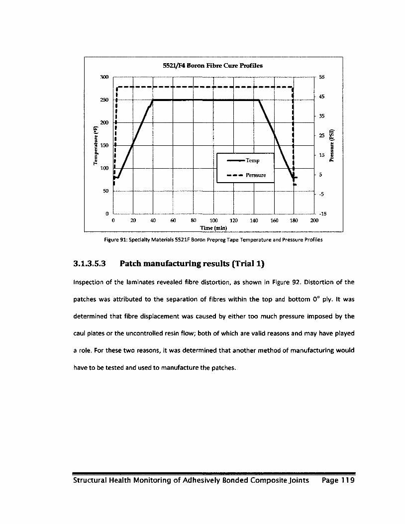
5521/F4 Boron Fibre Cure Profiles
20 40 60 80 100 120 140 160 180 200
Time (min)
Figure 91: Specialty Materials 5521F Boron Prepreg Tape Temperature and Pressure Profiles
3.1.3.5.3 Patch manufacturing results (Trial 1)
Inspection of the laminates revealed fibre distortion, as shown in Figure 92. Distortion of the
patches was attributed to the separation of fibres within the top and bottom 0° ply. It was
determined that fibre displacement was caused by either too much pressure imposed by the
caul plates or the uncontrolled resin flow; both of which are valid reasons and may have played
a role. For these two reasons, it was determined that another method of manufacturing would
have to be tested and used to manufacture the patches.
Structural Health Monitoring of Adhesively Bonded Composite Joints Page 119
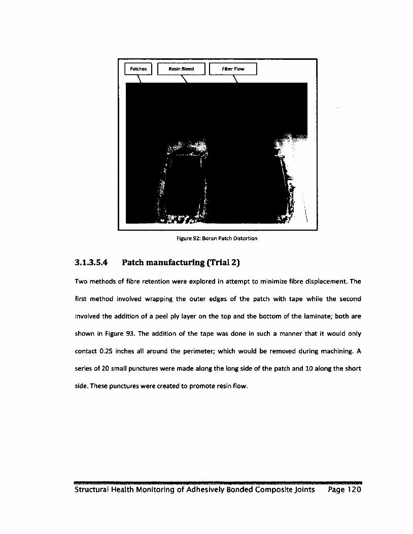
Patches Resin Bleed
Figure 92: Boron Patch Distortion
3.1.3.5.4 Patch manufacturing (Trial 2)
Two methods of fibre retention were explored in attempt to minimize fibre displacement. The
first method involved wrapping the outer edges of the patch with tape while the second
involved the addition of a peel ply layer on the top and the bottom of the laminate; both are
shown in Figure 93. The addition of the tape was done in such a manner that it would only
contact 0.25 inches all around the perimeter; which would be removed during machining. A
series of 20 small punctures were made along the long side of the patch and 10 along the short
side. These punctures were created to promote resin flow.
Structural Health Monitoring of Adhesively Bonded Composite Joints Page 120
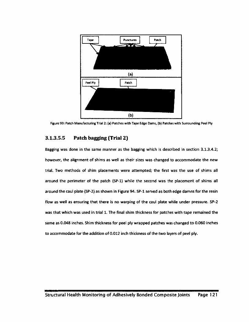
Punctures
Patch
Figure 93: Patch Manufacturing Trial 2: (a) Patches with Tape Edge Dams, (b) Patches with Surrounding Peel Ply
3.1.3.5.5 Patch bagging (Trial 2)
Bagging was done in the same manner as the bagging which is described in section 3.1.3.4.2;
however, the alignment of shims as well as their sizes was changed to accommodate the new
trial. Two methods of shim placements were attempted; the first was the use of shims all
around the perimeter of the patch (SP-1) while the second was the placement of shims all
around the caul plate (SP-2) as shown in Figure 94. SP-1 served as both edge damns for the resin
flow as well as ensuring that there is no warping of the caul plate while under pressure. SP-2
was that which was used in trial 1. The final shim thickness for patches with tape remained the
same as 0.048 inches. Shim thickness for peel ply wrapped patches was changed to 0.060 inches
to accommodate for the addition of 0.012 inch thickness of the two layers of peel ply.
Structural Health Monitoring of Adhesively Bonded Composite Joints Page 121
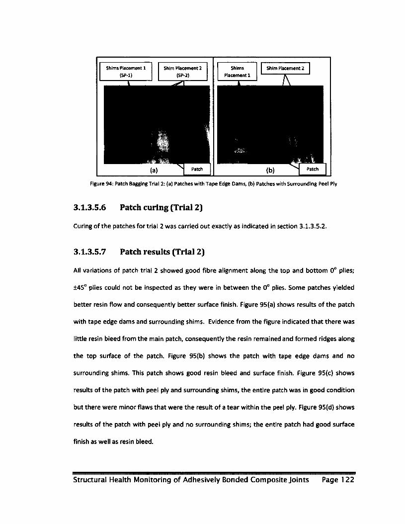
Shims Placement 1
(SP-1)
Shims
Placement 1
Shim Placement 2
(SP-2)
Shim Placement 2
Patch
Figure 94: Patch Bagging Trial 2: (a) Patches with Tape Edge Dams, (b) Patches with Surrounding Peel Ply
3.1.3.5.6 Patch curing (Trial 2)
Curing of the patches for trial 2 was carried out exactly as indicated in section 3.1.3.5.2.
3.1.3.5.7 Patch results (Trial 2)
All variations of patch trial 2 showed good fibre alignment along the top and bottom 0° plies;
±45° plies could not be inspected as they were in between the 0° plies. Some patches yielded
better resin flow and consequently better surface finish. Figure 95(a) shows results of the patch
with tape edge dams and surrounding shims. Evidence from the figure indicated that there was
little resin bleed from the main patch, consequently the resin remained and formed ridges along
the top surface of the patch. Figure 95(b) shows the patch with tape edge dams and no
surrounding shims. This patch shows good resin bleed and surface finish. Figure 95(c) shows
results of the patch with peel ply and surrounding shims, the entire patch was in good condition
but there were minor flaws that were the result of a tear within the peel ply. Figure 95(d) shows
results of the patch with peel ply and no surrounding shims; the entire patch had good surface
finish as well as resin bleed.
Structural Health Monitoring of Adhesively Bonded Composite Joints Page 122

Of all four patch variations, both taped edges and surrounding peel ply with SP-2 yielded better
surface finish and resin bleed as compared to patches utilizing SP-1. In anticipation of bonding
and its associated surface preparation for sensor instrumentation, the use of peel ply with no
surrounding shims was selected as the manufacturing method of choice. The use of peel ply
created a rough surface for sensors to adhere to as well as maintained a clean surface until
bonding procedures were carried out and peel ply layers removed.
Resin Ripples Resin Bleed Flaw Resin Bleed
(a) (b) (c) (d)
Figure 95: Patch Results Trial 2: (a) Patch with Tape Edge Dams and Surrounding Shims, (b) Patch with Tape Edge Dams and No Surrounding Shims, (c) Patch with Surrounding Peel Ply and Surrounding Shims and (d) Patch with
Surrounding Peel Ply and No Surrounding Shims
3.1.3.6 Patch to substrate bonding
This section describes the processes that were taken to bond the manufactured patches to the
manufactured substrates.
3.1.3.6.1 Bonding setup
Bonding of patches to the substrate was started by surface preparation of the substrate; this
was achieved by grit blasting the surface of the substrate where the patch was to be bonded as
shown in Figure 96(a). A single layer of FM73 film adhesive was cut to the size of the patch and
Structural Health Monitoring of Adhesively Bonded Composite Joints Page 123
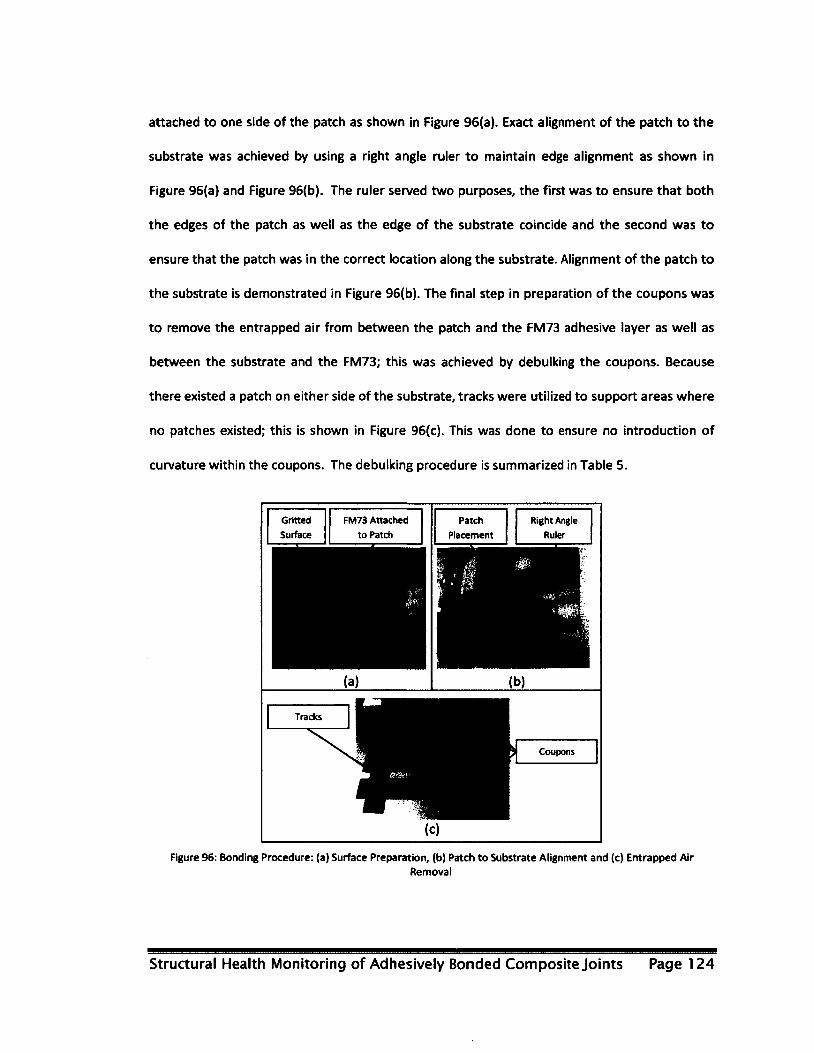
attached to one side of the patch as shown in Figure 96(a). Exact alignment of the patch to the
substrate was achieved by using a right angle ruler to maintain edge alignment as shown in
Figure 96(a) and Figure 96(b). The ruler served two purposes, the first was to ensure that both
the edges of the patch as well as the edge of the substrate coincide and the second was to
ensure that the patch was in the correct location along the substrate. Alignment of the patch to
the substrate is demonstrated in Figure 96(b). The final step in preparation of the coupons was
to remove the entrapped air from between the patch and the FM73 adhesive layer as well as
between the substrate and the FM73; this was achieved by debulking the coupons. Because
there existed a patch on either side of the substrate, tracks were utilized to support areas where
no patches existed; this is shown in Figure 96(c). This was done to ensure no introduction of
curvature within the coupons. The debulking procedure is summarized in Table 5.
Gritted
Surface
FM73 Attached
to Patch
Patch
Placement
Right Angle
Ruler
n Coupons
Figure 96: Bonding Procedure: (a) Surface Preparation, (b) Patch to Substrate Alignment and (c) Entrapped Air Removal
Structural Health Monitoring of Adhesively Bonded Composite Joints Page 124

Table 5: Bonding Debulking Procedure
Pressure Time 5 PSI 5 minutes 10 PSI 5 minutes 15 PSI 5 minutes 20 PSI 5 minutes 25 PSI 5 minutes or more
3.1.3.6.2 Coupon (final assembly) bagging
Due to the presence of a patch on either side of the coupon, the traditional bagging method
could not be applied; instead, an envelope bagging method was implemented. Envelope bagging
involves wrapping the coupon in the vacuum bag; this method allows all around pressure
distribution on the coupon.
In preparation of bagging, each coupon was individually wrapped with porous Teflon film as
shown in Figure 97(a). Each coupon was then placed onto the bag and separated with breather
cloth as shown in Figure 97(b); breather cloth was used so that a path for air is created such that
vacuum may be evenly applied to the coupon. Once sealed using sealant tape, vacuum was
pulled and pressure was applied on both sides of the coupon as shown in Figure 97(c).
Structural Health Monitoring of Adhesively Bonded Composite Joints Page 125
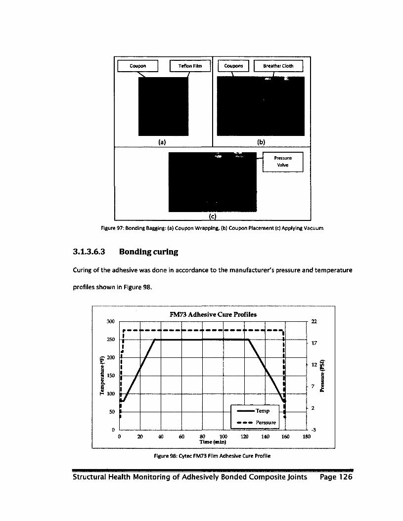
Teflon Film Coupons Breather Cloth Coupon
Pressure
Valve
Figure 97: Bonding Bagging: (a) Coupon Wrapping, (b) Coupon Placement (c) Applying Vacuum
3.1.3.6.3 Bonding curing
Curing of the adhesive was done in accordance to the manufacturer's pressure and temperature
profiles shown in Figure 98.
FM73 Adhesive Cure Profiles
20 40 60 80 100 120 140 160 180 Time (mill)
Figure 98: Cytec FM73 Film Adhesive Cure Profile
Structural Health Monitoring of Adhesively Bonded Composite Joints Page 126
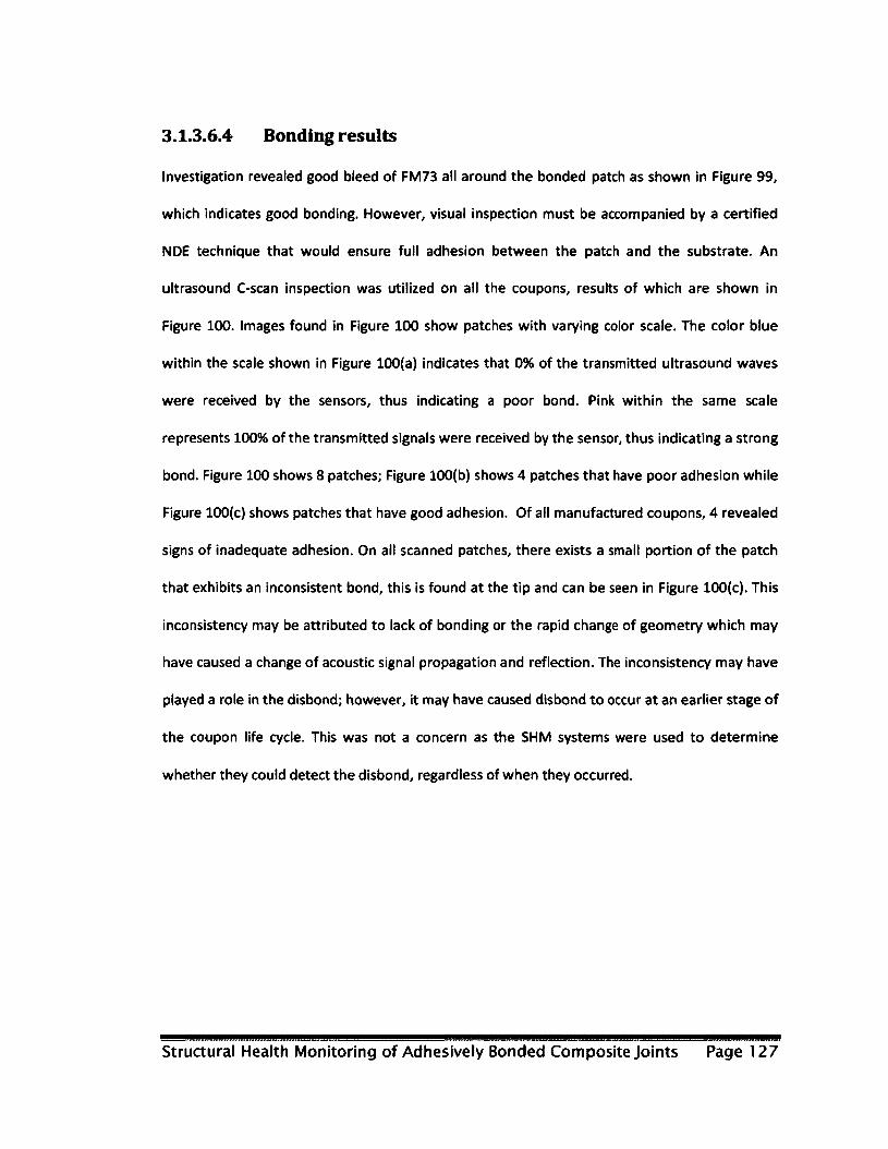
3.1.3.6.4 Bonding results
Investigation revealed good bleed of FM73 all around the bonded patch as shown in Figure 99,
which indicates good bonding. However, visual inspection must be accompanied by a certified
NDE technique that would ensure full adhesion between the patch and the substrate. An
ultrasound C-scan inspection was utilized on all the coupons, results of which are shown in
Figure 100. Images found in Figure 100 show patches with varying color scale. The color blue
within the scale shown in Figure 100(a) indicates that 0% of the transmitted ultrasound waves
were received by the sensors, thus indicating a poor bond. Pink within the same scale
represents 100% of the transmitted signals were received by the sensor, thus indicating a strong
bond. Figure 100 shows 8 patches; Figure 100(b) shows 4 patches that have poor adhesion while
Figure 100(c) shows patches that have good adhesion. Of all manufactured coupons, 4 revealed
signs of inadequate adhesion. On all scanned patches, there exists a small portion of the patch
that exhibits an inconsistent bond, this is found at the tip and can be seen in Figure 100(c). This
inconsistency may be attributed to lack of bonding or the rapid change of geometry which may
have caused a change of acoustic signal propagation and reflection. The inconsistency may have
played a role in the disbond; however, it may have caused disbond to occur at an earlier stage of
the coupon life cycle. This was not a concern as the SHM systems were used to determine
whether they could detect the disbond, regardless of when they occurred.
Structural Health Monitoring of Adhesively Bonded Composite Joints Page 127
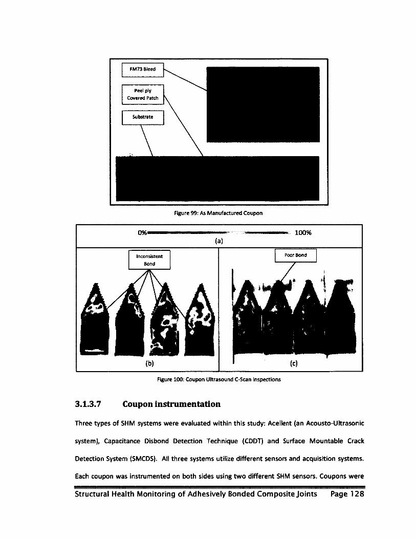
Figure 99: As Manufactured Coupon
100%
Inconsistent
Bond
Figure 100: Coupon Ultrasound C-Scan Inspections
3.1.3.7 Coupon instrumentation
Three types of SHM systems were evaluated within this study: Acellent (an Acousto-Ultrasonic
system), Capacitance Disbond Detection Technique (CDDT) and Surface Mountable Crack
Detection System (SMCDS). All three systems utilize different sensors and acquisition systems.
Each coupon was instrumented on both sides using two different SHM sensors. Coupons were
Structural Health Monitoring of Adhesively Bonded Composite Joints Page 128
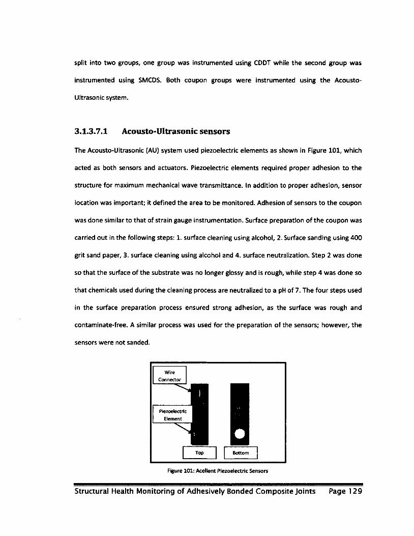
split into two groups, one group was instrumented using CDDT while the second group was
instrumented using SMCDS. Both coupon groups were instrumented using the Acousto-
Ultrasonic system.
3.1.3.7.1 Acousto-Ultrasonic sensors
The Acousto-Ultrasonic (AU) system used piezoelectric elements as shown in Figure 101, which
acted as both sensors and actuators. Piezoelectric elements required proper adhesion to the
structure for maximum mechanical wave transmittance. In addition to proper adhesion, sensor
location was important; it defined the area to be monitored. Adhesion of sensors to the coupon
was done similar to that of strain gauge instrumentation. Surface preparation of the coupon was
carried out in the following steps: 1. surface cleaning using alcohol, 2. Surface sanding using 400
grit sand paper, 3. surface cleaning using alcohol and 4. surface neutralization. Step 2 was done
so that the surface of the substrate was no longer glossy and is rough, while step 4 was done so
that chemicals used during the cleaning process are neutralized to a pH of 7. The four steps used
in the surface preparation process ensured strong adhesion, as the surface was rough and
contaminate-free. A similar process was used for the preparation of the sensors; however, the
sensors were not sanded.
Wire
Connector
Piezoel
Elem
Top Bottom
Figure 101: Acellent Piezoelectric Sensors
Structural Health Monitoring of Adhesively Bonded Composite Joints Page 129
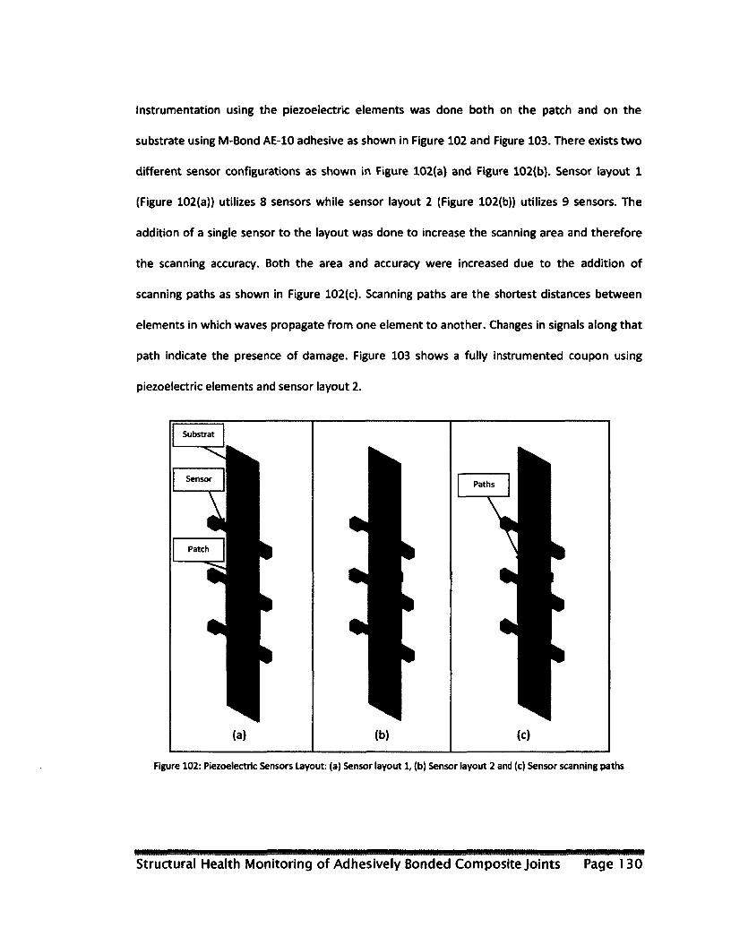
Instrumentation using the piezoelectric elements was done both on the patch and on the
substrate using M-Bond AE-10 adhesive as shown in Figure 102 and Figure 103. There exists two
different sensor configurations as shown in Figure 102(a) and Figure 102(b). Sensor layout 1
(Figure 102(a)) utilizes 8 sensors while sensor layout 2 (Figure 102(b)) utilizes 9 sensors. The
addition of a single sensor to the layout was done to increase the scanning area and therefore
the scanning accuracy. Both the area and accuracy were increased due to the addition of
scanning paths as shown in Figure 102(c). Scanning paths are the shortest distances between
elements in which waves propagate from one element to another. Changes in signals along that
path indicate the presence of damage. Figure 103 shows a fully instrumented coupon using
piezoelectric elements and sensor layout 2.
Substrat
Paths
Patch
Figure 102: Piezoelectric Sensors Layout: (a) Sensor layout 1, (b) Sensor layout 2 and (c) Sensor scanning paths
Structural Health Monitoring of Adhesively Bonded Composite Joints Page 130
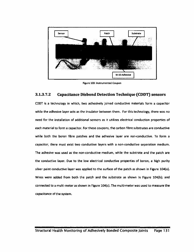
Sensor Patch Substrate
T\ m~7
M-10 Adhesive
Figure 103: Instrumented Coupon
3.1.3.7.2 Capacitance Disbond Detection Technique (CDDT) sensors
CDDT is a technology in which, two adhesively joined conductive materials form a capacitor
while the adhesive layer acts as the insulator between them. For this technology, there was no
need for the installation of additional sensors as it utilizes electrical conduction properties of
each material to form a capacitor. For these coupons, the carbon fibre substrates are conductive
while both the boron fibre patches and the adhesive layer are non-conductive. To form a
capacitor, there must exist two conductive layers with a non-conductive separation medium.
The adhesive was used as the non-conductive medium, while the substrate and the patch are
the conductive layer. Due to the low electrical conductive properties of boron, a high purity
silver paint conductive layer was applied to the surface of the patch as shown in Figure 104(a).
Wires were added from both the patch and the substrate as shown in Figure 104(b); and
connected to a multi-meter as shown in Figure 104(c). The multi-meter was used to measure the
capacitance of the system.
Structural Health Monitoring of Adhesively Bonded Composite Joints Page 131
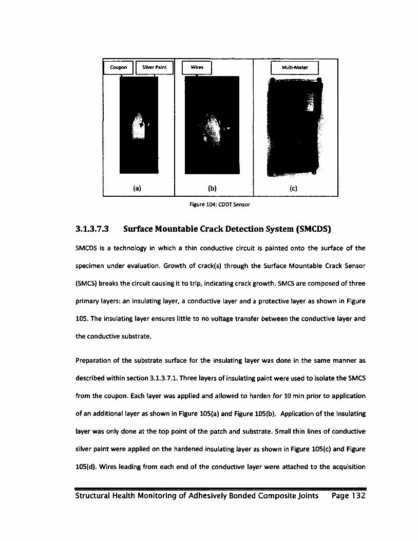
Coupon Silver Paint Wires Multi-Meter
(a)
"|
(b) (c)
Figure 104: CDDT Sensor
3.1.3.7.3 Surface Mountable Crack Detection System (SMCDS)
SMCDS is a technology in which a thin conductive circuit is painted onto the surface of the
specimen under evaluation. Growth of crack(s) through the Surface Mountable Crack Sensor
(SMCS) breaks the circuit causing it to trip, indicating crack growth. SMCS are composed of three
primary layers: an insulating layer, a conductive layer and a protective layer as shown in Figure
105. The insulating layer ensures little to no voltage transfer between the conductive layer and
the conductive substrate.
Preparation of the substrate surface for the insulating layer was done in the same manner as
described within section 3.1.3.7.1. Three layers of insulating paint were used to isolate the SMCS
from the coupon. Each layer was applied and allowed to harden for 10 min prior to application
of an additional layer as shown in Figure 105(a) and Figure 105(b). Application of the insulating
layer was only done at the top point of the patch and substrate. Small thin lines of conductive
silver paint were applied on the hardened insulating layer as shown in Figure 105(c) and Figure
105(d). Wires leading from each end of the conductive layer were attached to the acquisition
Structural Health Monitoring of Adhesively Bonded Composite Joints Page 132
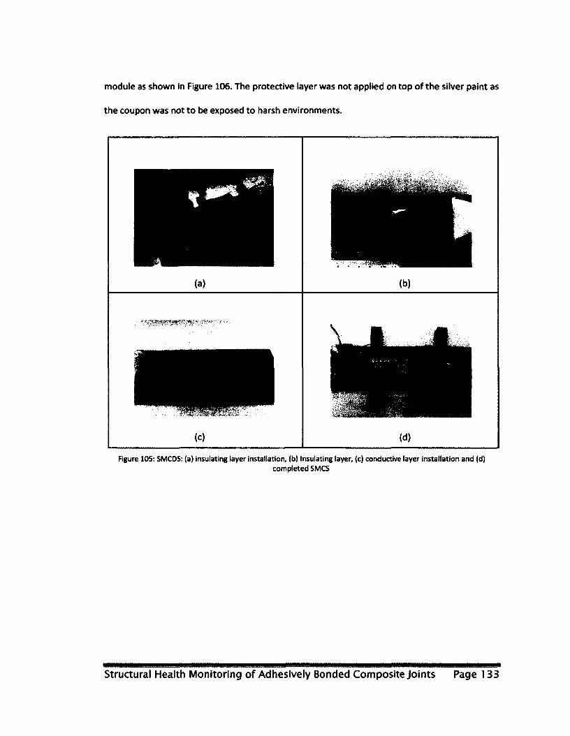
module as shown in Figure 106. The protective layer was not applied on top of the silver paint as
the coupon was not to be exposed to harsh environments.
Figure 105: SMCDS: (a) insulating layer installation, (b) Insulating layer, (c) conductive layer installation and (d) completed SMCS
Structural Health Monitoring of Adhesively Bonded Composite Joints Page 133
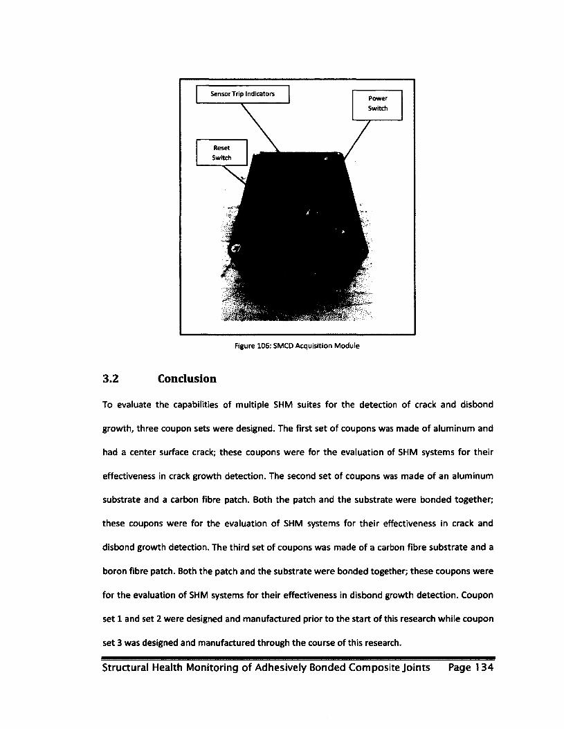
Sensor Trip Indicators Power
Switch
Reset
Switch
Figure 106: SMCD Acquisition Module
3.2 Conclusion
To evaluate the capabilities of multiple SHM suites for the detection of crack and disbond
growth, three coupon sets were designed. The first set of coupons was made of aluminum and
had a center surface crack; these coupons were for the evaluation of SHM systems for their
effectiveness in crack growth detection. The second set of coupons was made of an aluminum
substrate and a carbon fibre patch. Both the patch and the substrate were bonded together;
these coupons were for the evaluation of SHM systems for their effectiveness in crack and
disbond growth detection. The third set of coupons was made of a carbon fibre substrate and a
boron fibre patch. Both the patch and the substrate were bonded together; these coupons were
for the evaluation of SHM systems for their effectiveness in disbond growth detection. Coupon
set 1 and set 2 were designed and manufactured prior to the start of this research while coupon
set 3 was designed and manufactured through the course of this research.
Structural Health Monitoring of Adhesively Bonded Composite Joints Page 134

Coupon set 3 was designed to have a local area of high stress that would cause disbond within
that given region. This coupon design was done through the aid of ABAQUS* FEA software.
Three models were constructed within ABAQUS*: a conventional shell model, a continuum shell
model and a 3D stress model. The conventional shell model utilizes conventional shell elements
which are used to compute planar stresses. Through the use of these elements, computational
time was reduced as none of the out-of-plane stresses were calculated. This model was utilized
to quickly vary parameters within ply orientation, ply number and geometry in order to
determine the optimal coupon design solution. The continuum model was very similar to that
of the conventional shell model. Continuum elements do not allow for the calculations of out-of
plane stresses; however, unlike the conventional shell element, continuum elements may be
stacked through the thickness of the composite component. Results of this model were
compared with those obtained using conventional shell model. This model revealed that having
a single element through the thickness of each component was adequate for the computation of
stresses within the coupon. The 3D stress model was used to apply thermal loads which would
have been introduced during manufacturing and to determine if the applied mechanical load
would have overcome these thermal residual stresses. This model revealed that stresses within
the adhesive layer exceeded the strength of the adhesive and load application would cause a
disbond.
While manufacturing both the substrate and the patch, two issues were observed. The first was
the formation of bi-phase carbon fibre laminates and the second was fibre displacement within
the patches. Bi-phase laminates were formed as a result of slight misalignment of each ply
within the layup; this could have been avoided through experience; however, it does not pose a
problem for the evaluation of SHM technology. Fibre displacement did pose a problem for
experimentation as the patch stiffness was greatly influenced; for that reason trials were
Structural Health Monitoring of Adhesively Bonded Composite Joints Page 135

conducted to solve this issue. Trials revealed that applying a peel ply layer to either side of the
patch restricted the motion of fibres during resin flow.
Bonding of the patches to substrates was successful; however, ultrasound C-scans revealed that
4 of the manufactured coupons did not have adequate bonding. These 4 coupons were used for
testing as the experimentation was designed to detect disbond and not the strength of the
bond.
Acousto-Ultrasonic, CDDT and SMCDS where all instrumented on the coupons. Coupons where
split in two groups: SMCS were installed on one group and the CDDT sensors on the other group.
However, all coupons were instrumented with Acousto-Ultrasonic sensors.
Structural Health Monitoring of Adhesively Bonded Composite Joints Page 136

Chapter 4.0: Testing and Results
There were three coupon variants that were tested as part of this research. The first variant (Set
1) was of metallic construction and was designed for the evaluation of an Acousto-Ultrasonic
(AU) system for the detection of crack nucleation and growth. The second variant (Set 2), was of
metallic and composite construction. This second set was tested under two conditions for the
evaluation of the AU SHM system. The first condition was carried out to monitor the nucleation
and growth of adhesive failure between the composite and the metallic joint while the second
condition was to monitor adhesive failure as well as crack growth within the metallic substrate.
The third variant (Set 3) was of all-composite construction, in which a boron fibre patch was
adhesively bonded to a carbon fibre substrate. This final set was designed for the evaluation of
AU, Capacitive Disbond Detection Technique (CDDT) and Surface Mountable Crack Detection
System (SMCDS) for the detection of disbond between two composites.
As the AU SHM technology was the primary focus of this research, AU sensors were
instrumented on all coupon variants. CDDT and SMCDS were not evaluated on coupon Sets 1
and 2, as the designs were unsymmetrical (different patch designs on either side of the coupon)
and only allowed the evaluation of a single system. Coupon Set 3 however was of symmetric
design and therefore permitted the evaluation of two systems simultaneously. AU sensors were
instrumented on a single side while either CDDT or SMCDS were instrumented on the opposing
side.
For disbond of patches on coupon Set 2, coupons were subject to static loads for disbond to
occur. However, coupons were found to fail near the grips of the test frame and therefore, a
fatigue based approach was taken to cause disbond of the patch. There existed no off-the-shelf
software that could estimate the life of this coupon based on applied load and therefore loads
Structural Health Monitoring of Adhesively Bonded Composite Joints Page 137
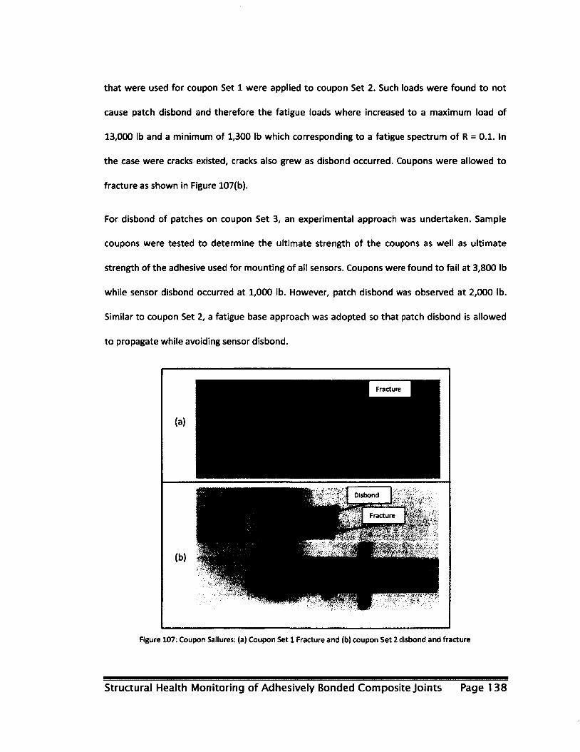
that were used for coupon Set 1 were applied to coupon Set 2. Such loads were found to not
cause patch disbond and therefore the fatigue loads where increased to a maximum load of
13,000 lb and a minimum of 1,300 lb which corresponding to a fatigue spectrum of R = 0.1. In
the case were cracks existed, cracks also grew as disbond occurred. Coupons were allowed to
fracture as shown in Figure 107(b).
For disbond of patches on coupon Set 3, an experimental approach was undertaken. Sample
coupons were tested to determine the ultimate strength of the coupons as well as ultimate
strength of the adhesive used for mounting of all sensors. Coupons were found to fail at 3,800 lb
while sensor disbond occurred at 1,000 lb. However, patch disbond was observed at 2,000 lb.
Similar to coupon Set 2, a fatigue base approach was adopted so that patch disbond is allowed
to propagate while avoiding sensor disbond.
Fracture
Disbond
•**"", 5] Fracture
lit!*?:
Figure 107: Coupon Sailures: (a) Coupon Set 1 Fracture and (b) coupon Set 2 disbond and fracture
Structural Health Monitoring of Adhesively Bonded Composite Joints Page 138

In total there were 19 coupons tested, 5 for Set 1,4 for Set 2 and 10 for Set 3. The exact testing
procedure, data acquisition and analysis are described within the following subsections.
However, not all tested coupons have been described, only the best and worst results are
presented within this thesis.
4.1 Metallic Coupon (Set 1)
For crack growth on coupon Set 1, initial crack size measurements were obtained using
ultrasound C-scans as well as a traveling microscope (a visual inspection technique). The larger
of the two crack measurements was inputted into the Air Force Growth (AFGROW) software.
AFGROW software uses a conservative approach to calculate fatigue life data based on stress
intensity factors, stresses and loading conditions. AFGROW software was used to produce crack
length versus life cycle data for multiple analysis using different applied stress conditions. The
use of AFGROW allowed for the determination of loads required to induce fracture of the
coupon within approximately 100,000 cycles. As a result of this analysis, coupons were fatigued
at a maximum load of 10,000 lb and a minimum load of 100 lb. Setup for testing under these
conditions is described in the following section.
4.1.1 Apparatus Setup
Coupons of Set 1 were tested under cyclic conditions with loads between 10,000 lb and 1000 lb
which correlate to 20,000 PSI and 2000 PSI, respectively. Inspection of the coupon's health for
this set was executed through the use of an AU SHM and a traveling microscope NDE systems.
Coupons were placed within a test frame and were mounted at two attachment points, one at
the top and the other at the bottom of the coupon. Grips used for the application of force were
Structural Health Monitoring of Adhesively Bonded Composite Joints Page 139
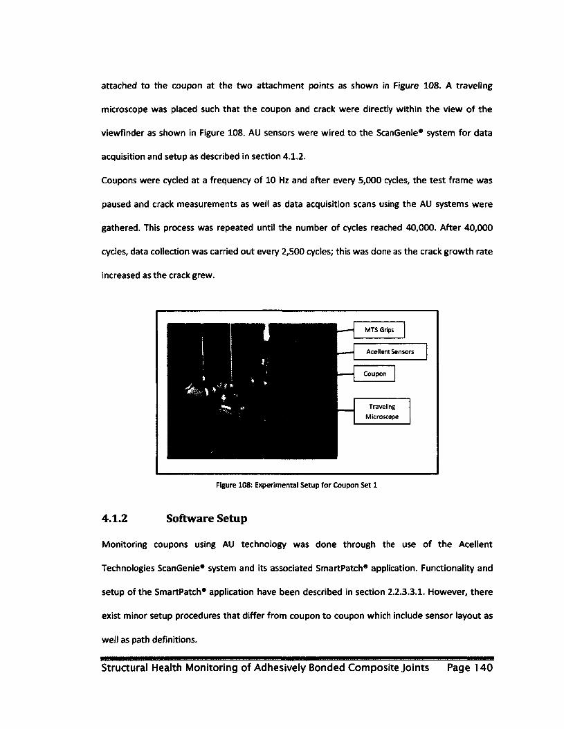
attached to the coupon at the two attachment points as shown in Figure 108. A traveling
microscope was placed such that the coupon and crack were directly within the view of the
viewfinder as shown in Figure 108. AU sensors were wired to the ScanGenie* system for data
acquisition and setup as described in section 4.1.2.
Coupons were cycled at a frequency of 10 Hz and after every 5,000 cycles, the test frame was
paused and crack measurements as well as data acquisition scans using the AU systems were
gathered. This process was repeated until the number of cycles reached 40,000. After 40,000
cycles, data collection was carried out every 2,500 cycles; this was done as the crack growth rate
increased as the crack grew.
Acellent Sensors
Coupon
Traveling
Microscope
Figure 108: Experimental Setup for Coupon Set 1
4.1.2 Software Setup
Monitoring coupons using AU technology was done through the use of the Acellent
Technologies ScanGenie* system and its associated SmartPatch* application. Functionality and
setup of the SmartPatch* application have been described in section 2.2.3.3.1. However, there
exist minor setup procedures that differ from coupon to coupon which include sensor layout as
well as path definitions.
Structural Health Monitoring of Adhesively Bonded Composite Joints Page 140
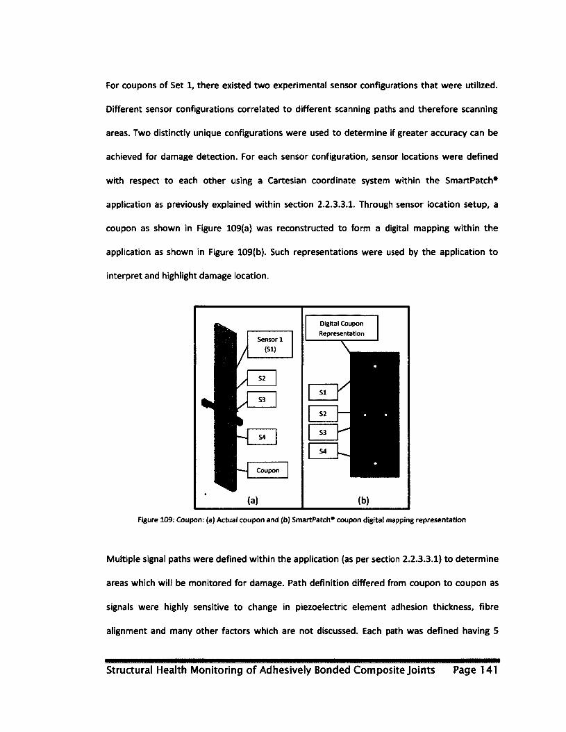
For coupons of Set 1, there existed two experimental sensor configurations that were utilized.
Different sensor configurations correlated to different scanning paths and therefore scanning
areas. Two distinctly unique configurations were used to determine if greater accuracy can be
achieved for damage detection. For each sensor configuration, sensor locations were defined
with respect to each other using a Cartesian coordinate system within the SmartPatch*
application as previously explained within section 2.2.3.3.1. Through sensor location setup, a
coupon as shown in Figure 109(a) was reconstructed to form a digital mapping within the
application as shown in Figure 109(b). Such representations were used by the application to
interpret and highlight damage location.
Digital Coupon
Representation
Coupon
Figure 109: Coupon: (a) Actual coupon and (b) SmartPatch* coupon digital mapping representation
Multiple signal paths were defined within the application (as per section 2.2.3.3.1) to determine
areas which will be monitored for damage. Path definition differed from coupon to coupon as
signals were highly sensitive to change in piezoelectric element adhesion thickness, fibre
alignment and many other factors which are not discussed. Each path was defined having 5
Structural Health Monitoring of Adhesively Bonded Composite Joints Page 141
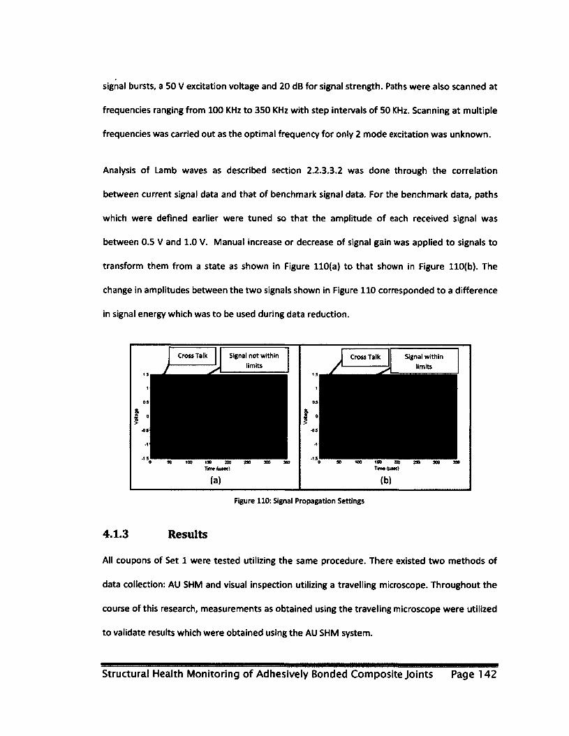
signal bursts, a 50 V excitation voltage and 20 dB for signal strength. Paths were also scanned at
frequencies ranging from 100 KHz to 350 KHz with step intervals of 50 KHz. Scanning at multiple
frequencies was carried out as the optimal frequency for only 2 mode excitation was unknown.
Analysis of Lamb waves as described section 2.2.3.3.2 was done through the correlation
between current signal data and that of benchmark signal data. For the benchmark data, paths
which were defined earlier were tuned so that the amplitude of each received signal was
between 0.5 V and 1.0 V. Manual increase or decrease of signal gain was applied to signals to
transform them from a state as shown in Figure 110(a) to that shown in Figure 110(b). The
change in amplitudes between the two signals shown in Figure 110 corresponded to a difference
in signal energy which was to be used during data reduction.
Cross Talk Signal not within
limits
Signal within
limits
100 ISO 300 Twmfwfc)
Figure 110: Signal Propagation Settings
4.1.3 Results
All coupons of Set 1 were tested utilizing the same procedure. There existed two methods of
data collection: AU SHM and visual inspection utilizing a travelling microscope. Throughout the
course of this research, measurements as obtained using the traveling microscope were utilized
to validate results which were obtained using the AU SHM system.
Structural Health Monitoring of Adhesively Bonded Composite Joints Page 142

The Acellent ScanGenie* (AU SHM) system was equipped with the SmartPatch* application for
the analysis of signal data. The SmartPatch* application utilized two separate diagnostic and
prognostic utilities: Direct Path Image (DPI) and Semi-Empirical Damage Sizing (SEDS) Utilities.
The DPI utilizes the digital representation of the coupon to identify the location of defects while
the SEDS utility interprets damage size. Each utility was run independent of the other and
therefore the results for each is presented independently in the following sections.
4.1.3.1 Direct Path Image (DPI) utility results
The DPI utility is a powerful tool which was designed to allow for quick assessment of damage
initiation. The DPI utility utilizes the digital mapping of the coupon and displays damage in the
form of discoloration as shown in Figure 112. Identification of damaged areas was done by
comparing current signal data to that of the benchmark signal data.
Coupons which were analysed using the DPI utility were subjected to crack growth from
approximately 0.2 inches in length to approximately 1.0 inch prior to full fracture. The DPI utility
identified crack severity and location through the use of a color gradient as shown in Figure 111.
The color gradient ranges from dark blue to dark red. The blue on the scale is considered
undamaged while red represents severe damage.
Results showing progression of damage are presented for two coupons: SPP2-12 and SPP2-15
within this section. Both coupons utilized the same 4 sensor configuration and therefore utilized
a very similar digital coupon representation. Multiple DPI utility images were captured
throughout the life of each coupon; each corresponding to a different crack length. DPI utility
images at 5K, 20K, 40K, 55K, 70K and 80K for SPP2-12 were captured and are presented within
Figure 112. Crack detection on the coupon was observed as a change of color at the center of
Structural Health Monitoring of Adhesively Bonded Composite Joints Page 143

the coupon where the crack resides. Progression of the crack was also observed as a change of
color from blue to yellow when examining images within Figure 112. Images on the left denote
smaller crack size as indicated by the crack measurement located at the top of the images while
images on the right denote larger crack measurements.
The second coupon (coupon SPP2-15) utilized the same sensor configuration as that used on the
first coupon (SPP2-12). DPI utility images for SPP2-15 were captured at 5K, 20K, 40K, 55K, 75K
and 80K and are presented in Figure 113. The crack was located between the two middle
sensors as indicated in Figure 113. Crack identification and severity was presented using the
same color gradient as that explained for coupon SPP2-12. Changes in crack severity were
observed from right to left within Figure 113. Unlike SPP2-12, crack identification for SPP2-15
was not as accurate. The crack which was located between the two centre sensors was
identified as being located just below the actual location as shown in Figure 113; making
location identification inaccurate.
The third and final coupon tested as part of this set was SPP2-26. SPP2-26 was equipped with a
completely different sensor configuration than SPP2-12 and SPP2-15. The sensor configuration
used on SPP2-26 utilized 8 sensors which were bonded to the aluminum. The use of 8 sensors as
opposed to 4 was done to determine if greater damage detection accuracy could be obtained.
During testing of the coupon, sensors disbonded from the aluminum; this occurred at less than
40,000 cycles. Due to sensor disbond, signal propagation properties were affected and therefore
current signals could not be evaluated using the benchmark signals. Images for SPP2-26 have
not been included below as they did not provide valuable data for the evaluation of the SHM
system.
Structural Health Monitoring of Adhesively Bonded Composite Joints Page 144
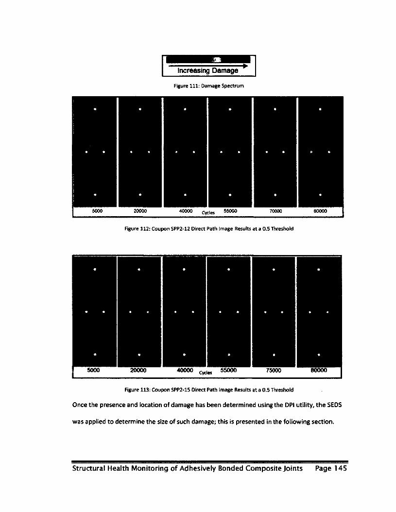
Increasing Damage *
Figure 111: Damage Spectrum
20000 40000 56000 80000 70000
Figure 112: Coupon SPP2-12 Direct Path Image Results at a 0.5 Threshold
20000 55000 40000 75000
Figure 113: Coupon SPP2-15 Direct Path Image Results at a 0.5 Threshold
Once the presence and location of damage has been determined using the DPI utility, the SEDS
was applied to determine the size of such damage; this is presented in the following section.
Structural Health Monitoring of Adhesively Bonded Composite Joints Page 145

4.1.3.2 Semi Empirical Damage Sizing (SEDS) results
The SEDS utility is one of the two utilities found within the SmartPatch* application and its
purpose was to determine crack lengths at all inspection points throughout the coupon life
cycle. The SEDS utility was able to analyze signal data and provided an "interpreted" damage
size; in this case, crack length. Interpreted crack lengths were a result of Damage Indices (Dl),
which were described in more detail within section 2.2.3.2. Damage Indices were obtained by
creating a Bspace file and by providing known crack lengths of the first few inspections to the
application. The Bspace is a collection of signal files into a single file or file database for which
current signals may be compared against for damage. For SPP2-12, SPP2-15 and SPP2-26
approximately 40% of all collected signal data was assigned to the Bspace file. Multiple analyses
were executed for each coupon, each with a different number of known crack length inputs.
For coupon SPP2-12, multiple analyses using the SEDS utility were executed, each with a
different known crack length inputs. Analysis for the interpretation of crack lengths was
executed with as little as 9 and as high as 21 known crack length inputs (as measured by the
traveling microscope). In total, there were 26 signal data files gathered for this coupon and the
SEDS utility was analyzing all signal data against the Bspace to determine crack lengths which
were not provided to the software. Figure 114 shows crack interpretations for analysis with 9
(40,000 cycle curve), 11 (45,000 cycle curve), 13 (50,000 cycle curve) and 17 (60,000 cycle curve)
crack length data point inputs. In addition to the analysis curves, two other curves exist: the
actual crack length as measured by the traveling microscope and AFGROW estimates. Recalling,
AFGROW software was used earlier to produce crack length versus life cycle data for each
coupon. While examining each of the curves produced by the SEDS utility within Figure 114, it is
evident that an increase in the number of known crack length inputs resulted in crack length
Structural Health Monitoring of Adhesively Bonded Composite Joints Page 146

interpretations that are closer to that of the actual measured crack lengths. All of the generated
SEDS curves were also found to over-interpret crack lengths; however, all such interpretations
were less than estimates produced using AFGROW. Within Figure 114, there existed one over-
interpreted point found at 55,000 cycles on all SEDS curves and is highlighted as an
"interpretation spike". The interpretation spike appeared to be an outlier as compared to all
other interpretations and may be a result of the polynomial approximations used within the
algorithm for the construction of the curves.
Similar to coupon SPP2-15, multiple analyses were executed using the SEDS utility, each with a
different quantity of known crack length inputs. Analyses for the interpretation of crack lengths
were executed with as little as 9 and as high as 20 known crack length inputs. In total, there
were 29 signal data files gathered for this coupon and the SEDS utility was used to determine
crack lengths which were not provided to the software. Figure 115 shows crack interpretations
for analysis with 11 (45,000 cycle curve), 15 (55,000 cycle curve), 19 (65,000 cycle curve) and 21
(70,000 cycle curve) crack length data point inputs. Similar to the results for SPP2-12, all the
SEDS curves were plotted along with the measured crack lengths as well as AFGROW estimates.
Examination of each of the curves produced by the SEDS utility within Figure 115 revealed the
same trend as that observed for coupon SPP2-12 within Figure 114. This trend indicates that an
increase in the number of known crack length inputs results in interpretations that are closer to
that of the actual measured crack length. Within Figure 115, there existed multiple
interpretation spikes which consistently over-predict the crack length. These multiple
interpretation spike may still be as a result of the polynomial approximations.
Structural Health Monitoring of Adhesively Bonded Composite Joints Page 147
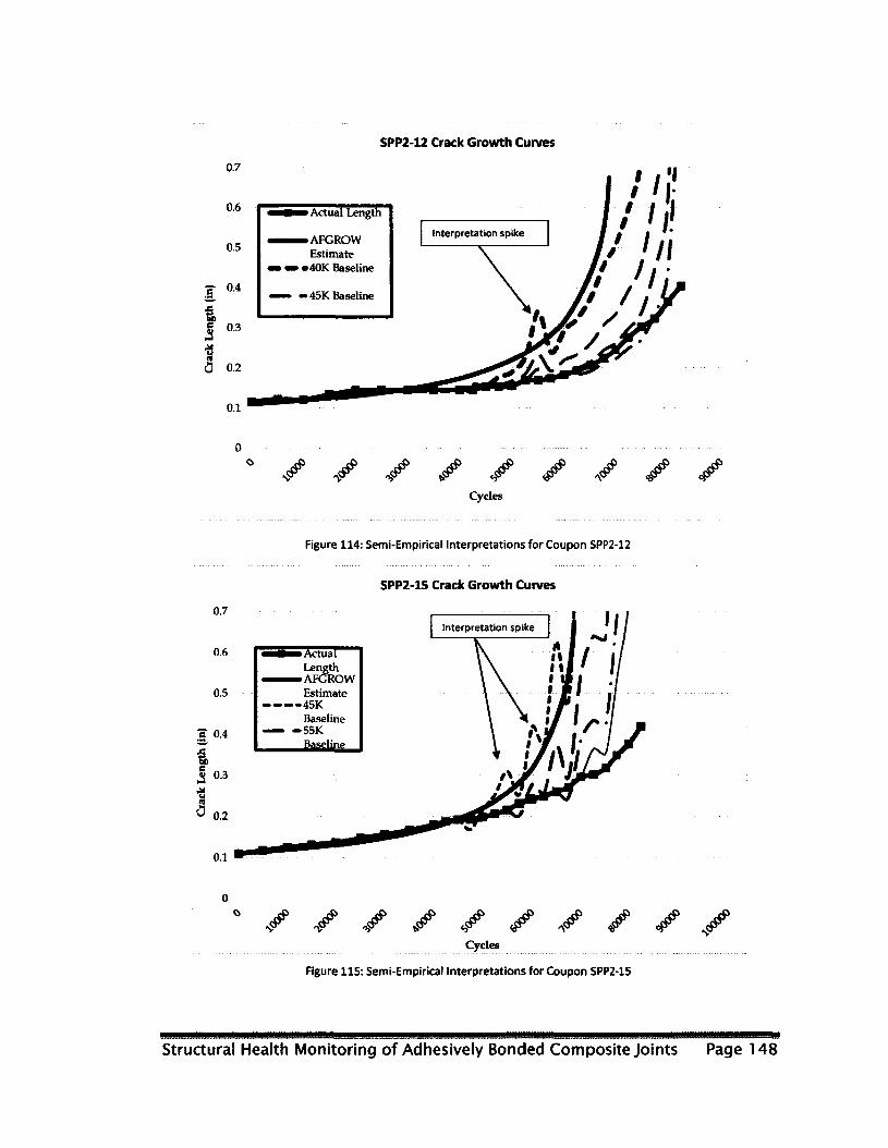
SPP2-12 Crack Growth Curves
•S
0.7
0.6
0.5
0.4
g 0.3
•B 3 0.2
•» Actual Length
—•AFGROW Estimate
» «40K Baseline
— 45K Baseline
Interpretation spike
I I V t * *
r / / i > n
y / y.
'/
o.i
<r
Cycles
Figure 114: Semi-Empirical Interpretations for Coupon SPP2-12
SPP2-15 Crack Growth Curves
0.7
0.6
0.5
I 0-4
0.2
0.1
Interpretation spike
Actual Length AFGROW Estimate 45K Baseline 55K
0.1
# •/ Cycles
Figure 115: Semi-Empirical Interpretations for Coupon SPP2-15
Structural Health Monitoring of Adhesively Bonded Composite Joints Page 148
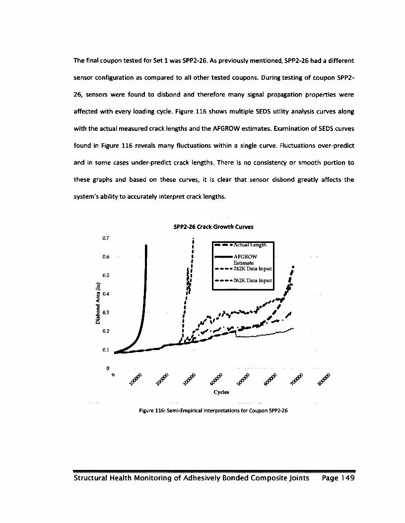
The final coupon tested for Set 1 was SPP2-26. As previously mentioned, SPP2-26 had a different
sensor configuration as compared to all other tested coupons. During testing of coupon SPP2-
26, sensors were found to disbond and therefore many signal propagation properties were
affected with every loading cycle. Figure 116 shows multiple SEDS utility analysis curves along
with the actual measured crack lengths and the AFGROW estimates. Examination of SEDS curves
found in Figure 116 reveals many fluctuations within a single curve. Fluctuations over-predict
and in some cases under-predict crack lengths. There is no consistency or smooth portion to
these graphs and based on these curves, it is clear that sensor disbond greatly affects the
system's ability to accurately interpret crack lengths.
SPP2-26 Crack Growth Curves
0.7
AFGROW Estimate 242K Data Input
0.6
0.5 262K Data Input
s 0.4
2 0.3
0.2
0.1
' • S s s s s s s s Cycles
Figure 116: Semi-Empirical Interpretations for Coupon SPP2-26
Structural Health Monitoring of Adhesively Bonded Composite Joints Page 149

4.2 Composite to Metallic (Coupon Set 2)
Coupons of Set 2 were designed for the evaluation of the AU SHM system for the detection of
disbond initiation and growth. This coupon set was intended to disbond under static loading;
however, during testing it was found that the coupons failed near the test frame grips. To
induce disbond, a fatigue based approach was utilized. Unlike coupon Set 1, there existed no
off-the-shelf software that was similar to AFGROW for estimation of disbond growth. These
coupons were initially loaded under the same conditions as those used for coupon Set 1. After
testing, disbond was not induced and the loads were changed to a maximum of 13,000 lb and a
minimum of 1,300 lb. Under these conditions the failure criteria was set such that 50% of the
patch was allowed to disbond. Setup for the testing under these parameters and conditions is
described in the following section.
4.2.1 Apparatus Setup
Coupons of Set 2 were tested under cyclic conditions with loads between 13,000 lb and 1300 lb
which correlate to 26,000 PSI and 2600 PSI, respectively. Inspection of coupon health for this set
was executed through the use of the AU SHM and the pulse thermography NDE systems.
Coupons were placed within the MTS test frame and were mounted at two attachment points
similar to that used for coupon Set 1 as shown in Figure 117. An infrared camera and two xenon
flashes (thermography system) were positioned such that the infrared camera was focused on
the patch as shown in Figure 117.
Coupons were cycled at a frequency of 10 Hz and after every 2,500 cycles, the test frame was
paused and thermography images as well as data acquisition scans using the AU system were
gathered. This process was repeated until the number of cycles reached 20,000. After 20,000
Structural Health Monitoring of Adhesively Bonded Composite Joints Page 1 50
cycles data collection was carried out every 5,000 cycles; this was done as disbond rates
decreased as the patch disbond area increased.
Software setup for the Acellent system was done in a similar manner as that used for coupon
Set 1 and as described in section 4.1.2.
Test Frame
Grips
Coupon
Pulsed
Thermography
Camera
Figure 117: Experimental Setup for Coupon Set 2
4.2.2 Results
A total of four coupons were tested as part of Set 2. All coupons were of carbon patch bonded
to an aluminum substrate design. Of all the manufactured coupons, three of the four coupons
had center surface cracks underneath the patch. All coupons of Set 2 were tested utilizing the
same procedure as described in section 4.2.1. There existed two methods of data collection
during testing: AU SHM and pulse thermograph NDE. Throughout the course of this research,
disbond area measurements were obtained using the thermography system and were used to
validate the results of the AU SHM system. For coupons with center surface cracks, crack lengths
were not validated as there were no means of obtaining the measurements without removal of
the coupon from the test frame.
Structural Health Monitoring of Adhesively Bonded Composite Joints Page 151
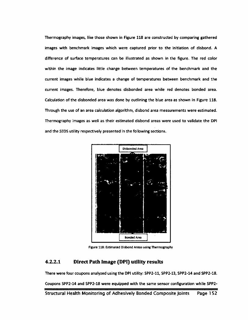
Thermography images, like those shown in Figure 118 are constructed by comparing gathered
images with benchmark images which were captured prior to the initiation of disbond. A
difference of surface temperatures can be illustrated as shown in the figure. The red color
within the image indicates little change between temperatures of the benchmark and the
current images while blue indicates a change of temperatures between benchmark and the
current images. Therefore, blue denotes disbonded area while red denotes bonded area.
Calculation of the disbonded area was done by outlining the blue area as shown in Figure 118.
Through the use of an area calculation algorithm, disbond area measurements were estimated.
Thermography images as well as their estimated disbond areas were used to validate the DPI
and the SEDS utility respectively presented in the following sections.
Disbonded Area
Bonded Area
Figure 118: Estimated Disbond Areas using Thermography
4.2.2.1 Direct Path Image (DPI) utility results
There were four coupons analyzed using the DPI utility: SPP2-11, SPP2-13, SPP2-14 and SPP2-18.
Coupons SPP2-14 and SPP2-18 were equipped with the same sensor configuration while SPP2-
Structural Health Monitoring of Adhesively Bonded Composite Joints Page 152
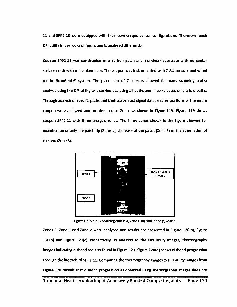
11 and SPP2-13 were equipped with their own unique sensor configurations. Therefore, each
DPI utility image looks different and is analysed differently.
Coupon SPP2-11 was constructed of a carbon patch and aluminum substrate with no center
surface crack within the aluminum. The coupon was instrumented with 7 AU sensors and wired
to the ScanGenie* system. The placement of 7 sensors allowed for many scanning paths;
analysis using the DPI utility was carried out using all paths and in some cases only a few paths.
Through analysis of specific paths and their associated signal data, smaller portions of the entire
coupon were analyzed and are denoted as Zones as shown in Figure 119. Figure 119 shows
coupon SPP2-11 with three analysis zones. The three zones shown in the figure allowed for
examination of only the patch tip (Zone 1), the base of the patch (Zone 2) or the summation of
the two (Zone 3).
Figure 119: SPP2-11 Scanning Zones: (a) Zone 1, (b) Zone 2 and (c) Zone 3
Zones 3, Zone 1 and Zone 2 were analyzed and results are presented in Figure 120(a), Figure
120(b) and Figure 120(c), respectively. In addition to the DPI utility images, thermography
images indicating disbond are also found in Figure 120. Figure 120(d) shows disbond progression
through the lifecycle of SPP2-11. Comparing the thermography images to DPI utility images from
Figure 120 reveals that disbond progression as observed using thermography images does not
Structural Health Monitoring of Adhesively Bonded Composite Joints Page 1 53

correlate with that indicated using Zone 3 analysis. Rather, Zone 3 analysis indicates large
disbond in as early as 40,000 cycles and is found beneath the entire surface of the patch.
However, Zone 1 analysis reveals that damage progression as indicated through the DPI utility
correlates to that of the thermography images and disbond location is indicated accurately.
Analysis of Zone 2 using DPI utility indicates disbond at the bottom side of the patch, which is
accurate. However, comparing Zone 1 and Zone 2 analysis to each other reveals that according
to the highlighted areas, disbond areas found in Zone 1 and Zone 2 should be identical in size;
this is however not true as thermography images show major disbond at the tip and little
disbond at the base.
Structural Health Monitoring of Adhesively Bonded Composite Joints Page 1 54
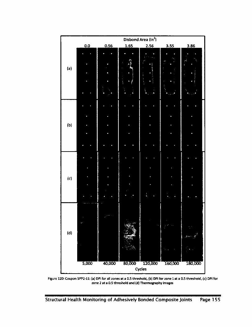
Disbond Area (in2)
0.0 0.56 1.65 2.56 3.55 3.86
5,000 40,000 80,000 120,000 160,000 180,000 Cycles
Figure 120: Coupon SPP2-11: (a) DPI for all zones at a 0.5 threshold, (b) DPI for zone 1 at a 0.5 threshold, (c) DPI for zone 2 at a 0.5 threshold and (d) Thermography images
Structural Health Monitoring of Adhesively Bonded Composite Joints Page 155

Coupon SPP2- 13 was the second coupon tested as part of this set; this coupon contained a
center surface crack underneath the bonded patch. For this coupon, two forms of damage
progression existed: patch disbond and crack growth. Coupon SPP2-13 had a different sensor
configuration than that of SPP2-14 and SPP2-18 which were of identical coupon design. The
sensor configuration used on SPP2-13 utilized 10 sensors which allowed for multi-zone analysis.
Four zones were analyzed using the DPI utility; Zone 1, Zone 2, Zone 3 and Zone 4 each of which
focuses on a specific section of the coupon. Zone 1, Zone 2, Zone 3 and Zone 4 focus on the tip
of the patch, the center of the patch, the base of the patch and the entire coupon respectively
as shown in Figure 121. DPI utility images for all zones along with thermography images are
presented in Figure 122. All DPI utility images as well as thermography images from Figure 122
were captured at 5,000, 20,000,40,000, 55,000, 70,000, and 80,000 cycles.
Each zone's DPI utility images were analysed independently and obtained results were
compared to thermography images for validation. Examination of Zone 4 DPI utility images for
all cycles indicates disbond of the entire patch in as early as 55,000 cycles; however, the largest
captured disbond area as validated by thermography and shown in Figure 122 occurs at 80,000
cycles. Examination of Zone 1 and comparing its results to the thermography images reveals that
there is a correlation between the actual disbond area and the disbond area as indicated by the
DPI utility. Increase in disbond area is accurately indicated in the location of the patch tip with
varying intensity as shown in Figure 122(b). Unlike results for Zone 1, results for Zone 2 are
influenced by both crack growth as well as disbond. Zone 2 images are shown in Figure 122(c)
and indicate significant damage formation while thermography images show no disbond in that
region prior to 70,000 cycles. The damage formation as indicated within Zone 2 could be
attributed to crack growth alone; however, results are inconclusive as they were not validated
using an NDE system. Zone 3, was the final zone analysed for this coupon. Zone 3 focused on
Structura l Heal th Moni tor ing of Adhesively Bonded Composi te Joints Page 156
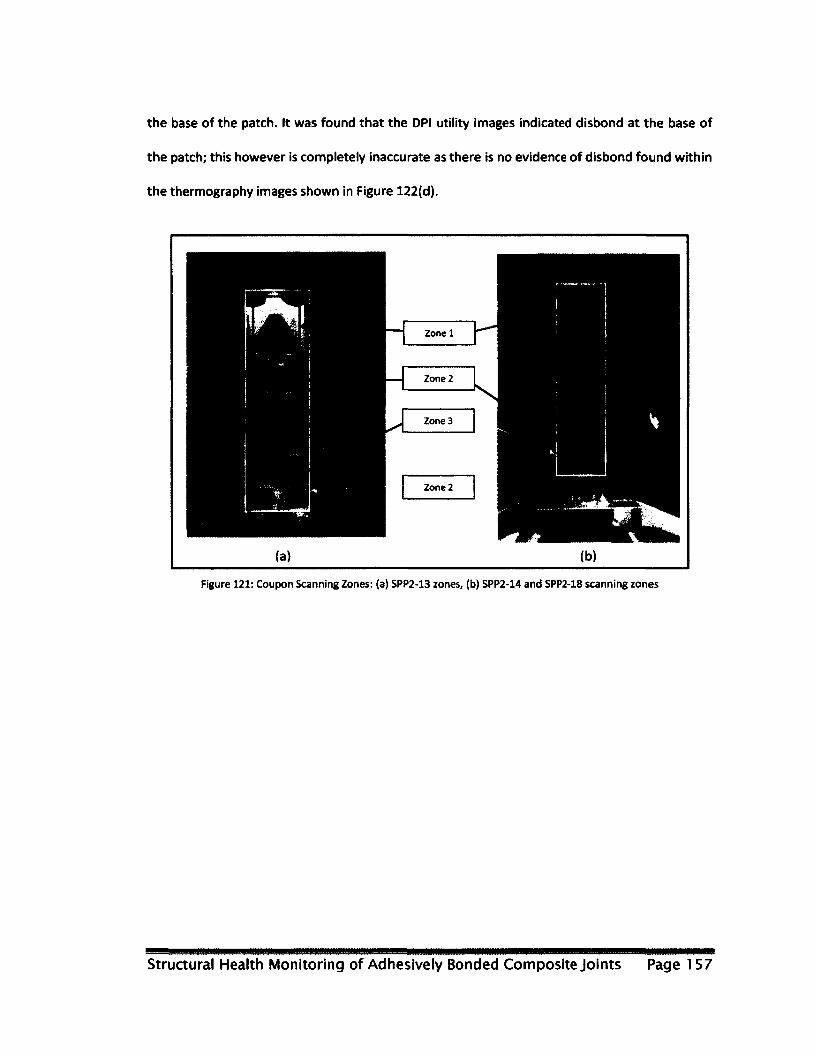
the base of the patch. It was found that the DPI utility images indicated disbond at the base of
the patch; this however is completely inaccurate as there is no evidence of disbond found within
the thermography images shown in Figure 122(d).
Figure 121: Coupon Scanning Zones: (a) SPP2-13 zones, (b) SPP2-14 and SPP2-18 scanning zones
Structural Health Monitoring of Adhesively Bonded Composite Joints Page 1 57
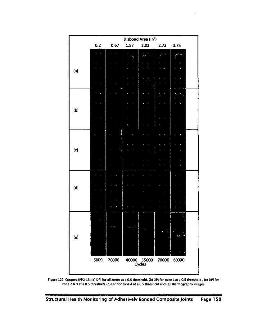
Disbond Area (in2)
0.2 0.67 1.57 2.02 2.72 3.75
5000 20000 40000 55000 70000 80000 Cycles
Figure 122: Coupon SPP2-13: (a) DPI for all zones at a 0.5 threshold, (b) DPI for zone 1 at a 0.5 threshold, (c) DPI for zone 2 & 3 at a 0.5 threshold, (d) DPI for zone 4 at a 0.5 threshold and (e) Thermography images
Structural Health Monitoring of Adhesively Bonded Composite Joints Page 158

Coupon SPP2-14 and SPP2-18 were the final two coupons tested within this set; both were
equipped with 6 sensors and an identical sensor configuration. The use of a 6 sensor
configuration allowed for multi-zone analysis. Similar to coupon SPP2-13, both of these coupons
experienced both crack growth and patch disbond. The 6 sensors were used to monitor three
zones. Zone 1, Zone 2 and Zone 3 focus on the tip of the patch, the base of the patch and the
entire coupon, respectively, and are all shown in Figure 121. The DPI utility images for all zone
analyses as well as thermography images for coupon SPP2-14 are shown in Figure 123; the DPI
utility images for SPP2-18 are not presented within this chapter as they are similar to those of
SPP2-14.
Each zone's DPI utility images were analysed independently and results of which were compared
to thermography images for validation. Examination of Zone 3 DPI utility images for all cycles
indicates disbond of the entire patch in as early as 40,000 cycles. However, the largest captured
disbond area as validated by thermography and as shown in Figure 123(d) occurs at 80,000
cycles and is approximately 20% of the overall patch area. Examination of Zone 1, while
comparing its results to the thermography images, reveals that there is a correlation between
the actual disbond area and the disbond area as indicated by the DPI utility. Increase in disbond
area is indicated in the location of the tip of the patch with varying intensity as shown in Figure
123(a). Zone 2, was the final zone analysed for this coupon. Zone 2 focused on the base of the
patch. It was found that the DPI utility images indicated disbond at the base of the patch; this
however is completely inaccurate as there is no evidence of disbond found within the
thermography images shown in Figure 123(d).
Structural Health Monitoring of Adhesively Bonded Composite Joints Page 159

After examining coupons SPP2-11, SPP2-13, SPP2-14 and SPP2-18 using the DPI utility for
damage identification, the SEDS was applied to determine the size of such damage; this is
presented in the following section.
Structural Health Monitoring of Adhesively Bonded Composite Joints Page 160
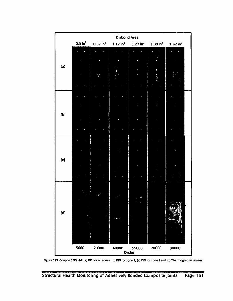
Disbond Area
0.0 in2 0.69 in2 1.17 in2 1.27 in2 1.39 in2 1.82 in2
5000 20000 40000 55000 70000 80000 Cycles
Figure 123: Coupon SPP2-14: (a) DPI for all zones, (b) DPI for zone 1, (c) DPI for zone 2 and (d) Thermography images
Structural Health Monitoring of Adhesively Bonded Composite Joints Page 161

4.2.2.2 Semi Empirical Damage Sizing (SEDS) Results
The SEDS utility is one of the two utilities found within the SmartPatch* application and its
purpose was determining disbond area at all inspection points throughout the coupon life cycle.
The SEDS utility was able to analyze signal data and provides an "interpreted" damage size; in
this case, disbond area. Interpreted disbond areas are a result of Damage Indices (Dl), which
were described in more detail within section 2.2.3.2. Damage Indices were obtained by creating
a Bspace file and via providing known disbond areas for the first few inspections to the
application. For SPP2-11, SPP2-13, SPP2-14 and SPP2-18 approximately 40% of all collected
signal data was assigned to the Bspace file. Multiple analyses were executed for each coupon,
each with a different number of known disbond area inputs.
For coupon SPP2-11 multiple analyses using the SEDS utility were executed, each with different
known disbond area inputs. Analyses for the interpretation of disbond area were executed with
as little as 13 and as high as 41 known disbond area inputs (as found using thermography). In
total, there were 49 signal data files gathered for this coupon and the SEDS utility was analysing
all signal data against the Bspace to determine disbond areas which were not provided to the
software. Figure 124 shows disbond area interpretations for analysis with 24 (95,000 cycle
curve), 27 (110,000 cycle curve), 32 (135,000 cycle curve) and 41 (185,000 cycle curve) disbond
area data point inputs. In addition to the SEDS curves, the actual disbond area curve is also
plotted within Figure 124. While examining each of the curves produced by the SEDS utility
within Figure 124, it is evident that an increase in the number of known disbond area inputs
results in interpretations that are closer to that of the actual measured value. Unlike the results
for coupons of Set 1, results of SEDS interpretations are inaccurate by a minimum of 45% and a
Structural Health Monitoring of Adhesively Bonded Composite Joints Page 162
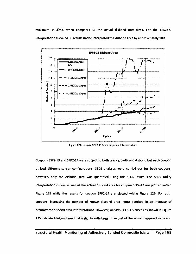
maximum of 375% when compared to the actual disbond area sizes. For the 185,000
interpretation curve, SEDS results under-interpreted the disbond area by approximately 10%.
SPP2-11 Disbond Area
20
18
16
14
ft
a 12 1 < 10 •u 6 O • 8 S
6
4
2
0
—
Disbond Area (in2)
— • 95K Datalnput
110K Datalnput
135K Datalnput
• • • 185K Datalnput
/ A / • -N .
—
Disbond Area (in2)
— • 95K Datalnput
110K Datalnput
135K Datalnput
• • • 185K Datalnput —
Disbond Area (in2)
— • 95K Datalnput
110K Datalnput
135K Datalnput
• • • 185K Datalnput
r J
—
Disbond Area (in2)
— • 95K Datalnput
110K Datalnput
135K Datalnput
• • • 185K Datalnput
•
A / —
Disbond Area (in2)
— • 95K Datalnput
110K Datalnput
135K Datalnput
• • • 185K Datalnput
" 1 • • • 1 V M —
Disbond Area (in2)
— • 95K Datalnput
110K Datalnput
135K Datalnput
• • • 185K Datalnput 1 v
/. V
—
/ I * * V' ̂ •
, as* — w *
I - " 1 • •
— w *
Cycles
Figure 124: Coupon SPP2-11 Semi-Empirical Interpretations
Coupons SSP2-13 and SPP2-14 were subject to both crack growth and disbond but each coupon
utilized different sensor configurations. SEDS analyses were carried out for both coupons;
however, only the disbond area was quantified using the SEDS utility. The SEDS utility
interpretation curves as well as the actual disbond area for coupon SPP2-13 are plotted within
Figure 125 while the results for coupon SPP2-14 are plotted within Figure 126. For both
coupons, increasing the number of known disbond area inputs resulted in an increase of
accuracy for disbond area interpretations. However, all SPP2-13 SEDS curves as shown in Figure
125 indicated disbond area that is significantly larger than that of the actual measured value and
Structural Health Monitoring of Adhesively Bonded Composite Joints Page 163
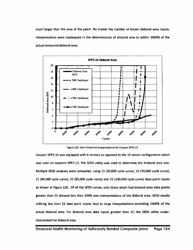
much larger than the area of the patch. No matter the number of known disbond area inputs,
interpretations were inadequate in the determination of disbond area to within 1000% of the
actual measured disbond area.
SPP2-13 Disbond Area
20
18
16
14
1 2
? »
I . 6 o 8 6
Q
• Disbond Area (in2)
50K Datalnput
• 60K Datalnput
»70K Datalnput
• 75K Datalnput
Figure 125: Semi-Empirical Interpretations for Coupon SPP2-13
Coupon SPP2-14 was equipped with 6 sensors as opposed to the 10 sensor configuration which
was used on coupons SPP2-13. The SEDS utility was used to determine the disbond area size.
Multiple SEDS analyses were computed, using 15 (50,000 cycle curve), 19 (70,000 cycle curve),
21 (80,000 cycle curve), 22 (85,000 cycle curve) and 25 (100,000 cycle curve) data point inputs
as shown in Figure 126. Of all the SEDS curves, only those which had disbond area data points
greater than 22 showed less than 200% over-interpretations of the disbond area. SEDS results
utilizing less than 22 data point inputs lead to large interpretations exceeding 1000% of the
actual disbond area. For disbond area data inputs greater than 25, the SEDS utility under-
interpreted the disbond area.
Structural Health Monitoring of Adhesively Bonded Composite Joints Page 164
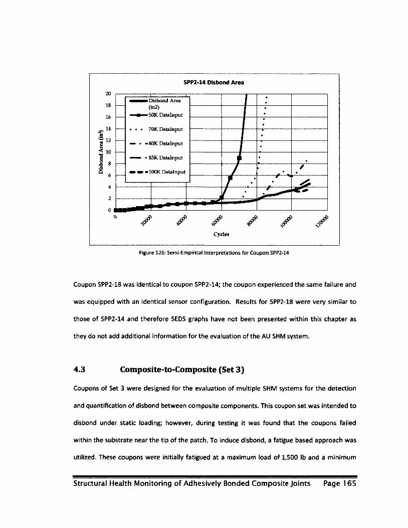
SPP2-14 Disbond Area
Disbond Area (in2) 50K Datalnput
70K Datalnput
80K Datalnput
85K Datalnput
• 100K Datalnput
Figure 126: Semi-Empirical Interpretations for Coupon SPP2-14
Coupon SPP2-18 was identical to coupon SPP2-14; the coupon experienced the same failure and
was equipped with an identical sensor configuration. Results for SPP2-18 were very similar to
those of SPP2-14 and therefore SEDS graphs have not been presented within this chapter as
they do not add additional information for the evaluation of the AU SHM system.
4.3 Composite-to-Composite (Set 3)
Coupons of Set 3 were designed for the evaluation of multiple SHM systems for the detection
and quantification of disbond between composite components. This coupon set was intended to
disbond under static loading; however, during testing it was found that the coupons failed
within the substrate near the tip of the patch. To induce disbond, a fatigue based approach was
utilized. These coupons were initially fatigued at a maximum load of 1,500 lb and a minimum
Structural Health Monitoring of Adhesively Bonded Composite Joints Page 165
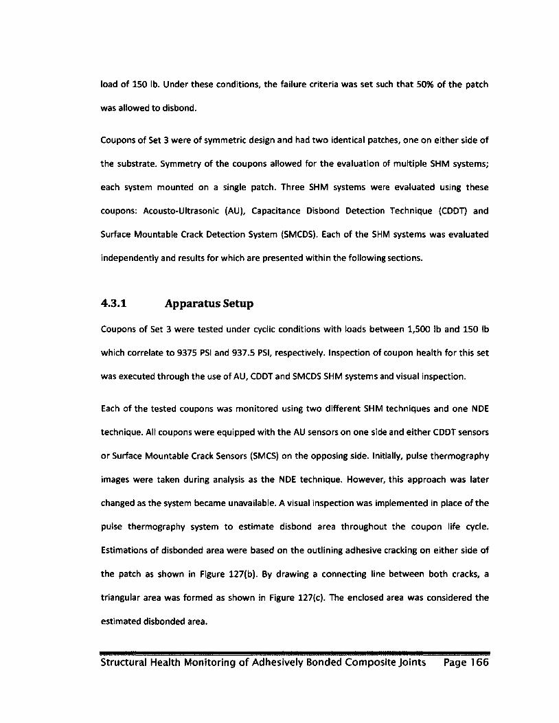
load of 150 lb. Under these conditions, the failure criteria was set such that 50% of the patch
was allowed to disbond.
Coupons of Set 3 were of symmetric design and had two identical patches, one on either side of
the substrate. Symmetry of the coupons allowed for the evaluation of multiple SHM systems;
each system mounted on a single patch. Three SHM systems were evaluated using these
coupons: Acousto-Ultrasonic (AU), Capacitance Disbond Detection Technique (CDDT) and
Surface Mountable Crack Detection System (SMCDS). Each of the SHM systems was evaluated
independently and results for which are presented within the following sections.
4.3.1 Apparatus Setup
Coupons of Set 3 were tested under cyclic conditions with loads between 1,500 lb and 150 lb
which correlate to 9375 PSI and 937.5 PSI, respectively. Inspection of coupon health for this set
was executed through the use of AU, CDDT and SMCDS SHM systems and visual inspection.
Each of the tested coupons was monitored using two different SHM techniques and one NDE
technique. All coupons were equipped with the AU sensors on one side and either CDDT sensors
or Surface Mountable Crack Sensors (SMCS) on the opposing side. Initially, pulse thermography
images were taken during analysis as the NDE technique. However, this approach was later
changed as the system became unavailable. A visual inspection was implemented in place of the
pulse thermography system to estimate disbond area throughout the coupon life cycle.
Estimations of disbonded area were based on the outlining adhesive cracking on either side of
the patch as shown in Figure 127(b). By drawing a connecting line between both cracks, a
triangular area was formed as shown in Figure 127(c). The enclosed area was considered the
estimated disbonded area.
Structural Health Monitoring of Adhesively Bonded Composite Joints Page 166
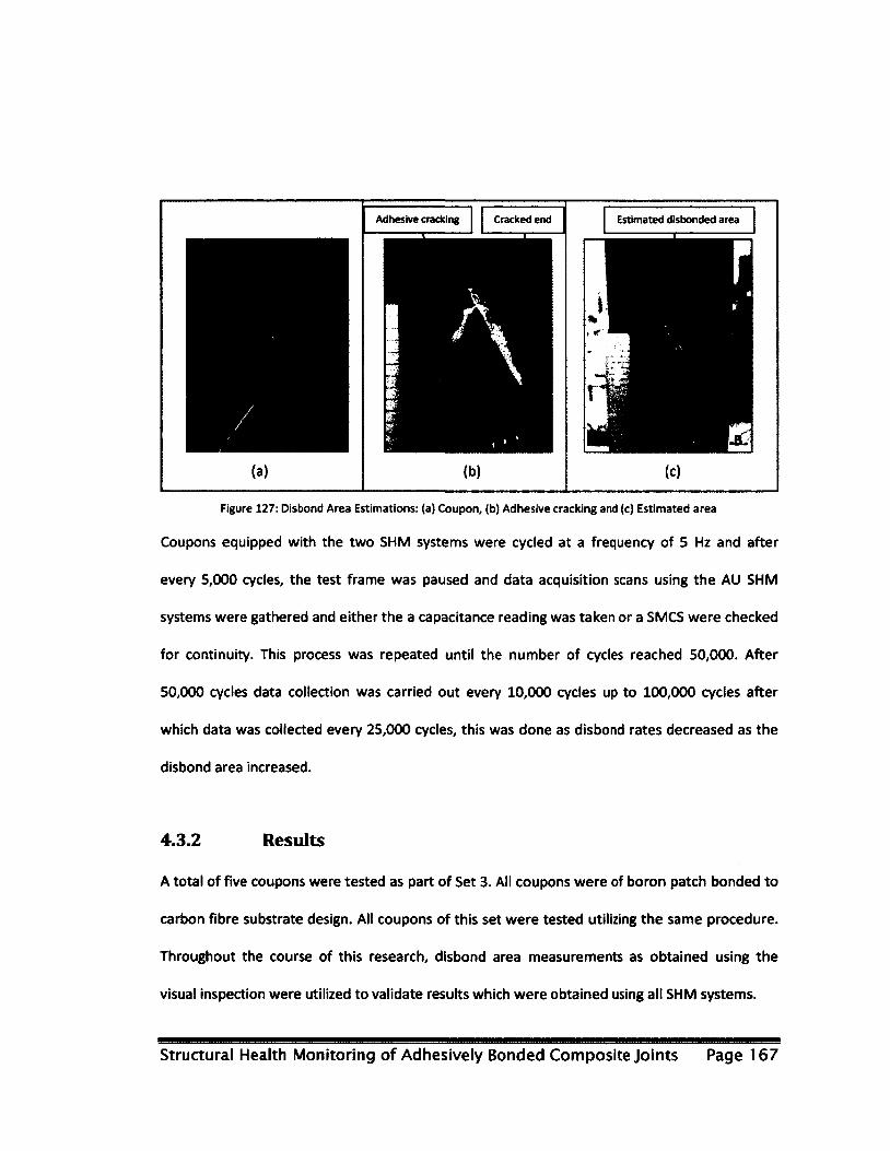
Adhesive cracking Cracked end Estimated disbonded area
Figure 127: Disbond Area Estimations: (a) Coupon, (b) Adhesive cracking and (c) Estimated area
Coupons equipped with the two SHM systems were cycled at a frequency of 5 Hz and after
every 5,000 cycles, the test frame was paused and data acquisition scans using the AU SHM
systems were gathered and either the a capacitance reading was taken or a SMCS were checked
for continuity. This process was repeated until the number of cycles reached 50,000. After
50,000 cycles data collection was carried out every 10,000 cycles up to 100,000 cycles after
which data was collected every 25,000 cycles, this was done as disbond rates decreased as the
disbond area increased.
4.3.2 Results
A total of five coupons were tested as part of Set 3. All coupons were of boron patch bonded to
carbon fibre substrate design. All coupons of this set were tested utilizing the same procedure.
Throughout the course of this research, disbond area measurements as obtained using the
visual inspection were utilized to validate results which were obtained using all SHM systems.
Structural Health Monitoring of Adhesively Bonded Composite Joints Page 167
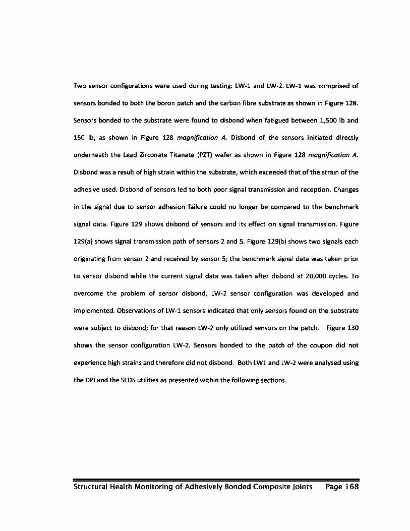
Two sensor configurations were used during testing: LW-1 and LW-2. LW-1 was comprised of
sensors bonded to both the boron patch and the carbon fibre substrate as shown in Figure 128.
Sensors bonded to the substrate were found to disbond when fatigued between 1,500 lb and
150 ib, as shown in Figure 128 magnification A. Disbond of the sensors initiated directly
underneath the Lead Zirconate Titanate (PZT) wafer as shown in Figure 128 magnification A.
Disbond was a result of high strain within the substrate, which exceeded that of the strain of the
adhesive used. Disbond of sensors led to both poor signal transmission and reception. Changes
in the signal due to sensor adhesion failure could no longer be compared to the benchmark
signal data. Figure 129 shows disbond of sensors and its effect on signal transmission. Figure
129(a) shows signal transmission path of sensors 2 and 5. Figure 129(b) shows two signals each
originating from sensor 2 and received by sensor 5; the benchmark signal data was taken prior
to sensor disbond while the current signal data was taken after disbond at 20,000 cycles. To
overcome the problem of sensor disbond, LW-2 sensor configuration was developed and
implemented. Observations of LW-1 sensors indicated that only sensors found on the substrate
were subject to disbond; for that reason LW-2 only utilized sensors on the patch. Figure 130
shows the sensor configuration LW-2. Sensors bonded to the patch of the coupon did not
experience high strains and therefore did not disbond. Both LW1 and LW-2 were analysed using
the DPI and the SEDS utilities as presented within the following sections.
Structural Health Monitoring of Adhesively Bonded Composite Joints Page 168
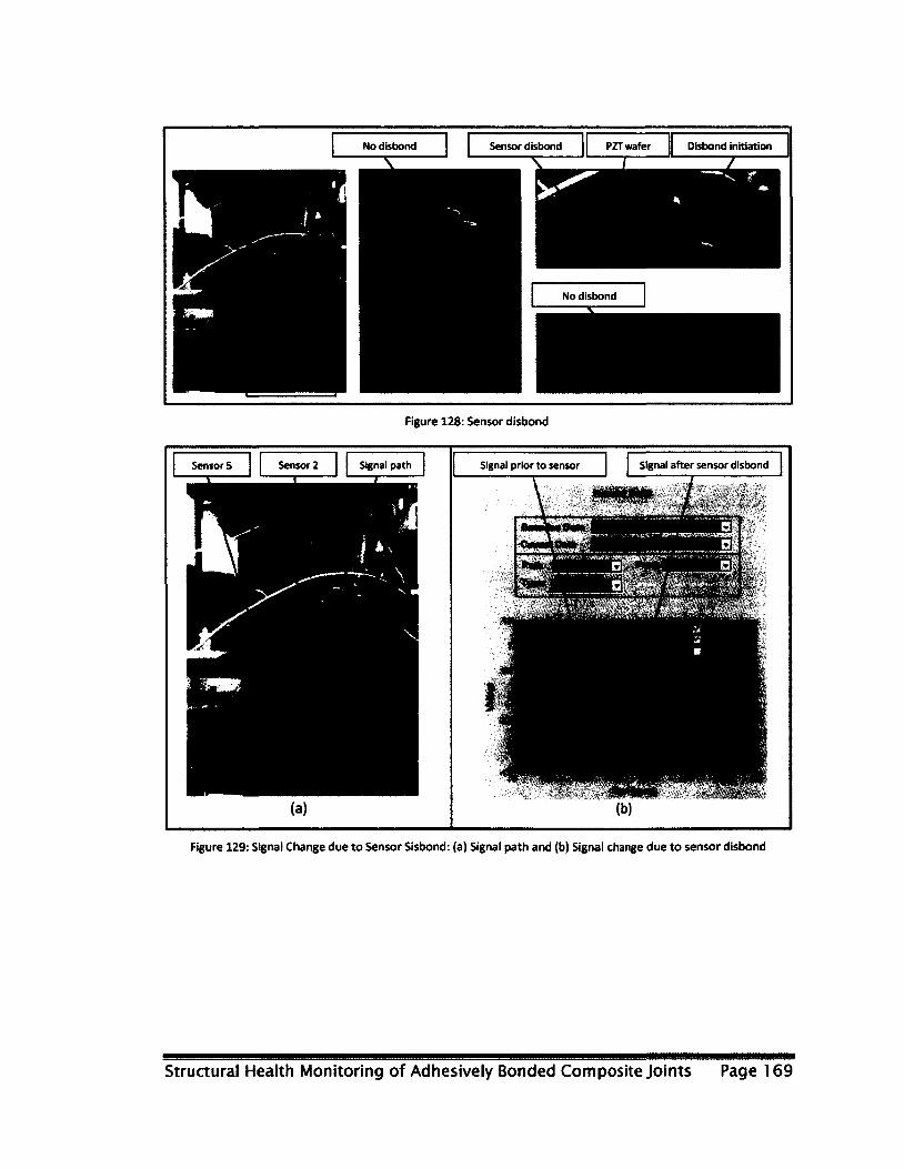
No disbond Sensor disbond PZT wafer Disbond initiation
No disbond
Figure 128: Sensor disbond
Signal after sensor disbond
Figure 129: Signal Change due to Sensor Sisbond: (a) Signal path and (b) Signal change due to sensor disbond
Structural Health Monitoring of Adhesively Bonded Composite Joints Page 169
Figure 130: Sensor Configuration Modification
4.3.2.1 Direct Path Image (DPI) utility results
There were five coupons analyzed using the DPI utility: three of which used LW-1 and the other
two used LW-2 sensor configurations. SPP3-03, SPP3-04 and SP3-16 utilized LW-1 while SPP3-4a
and SPP3-12 utilized LW-2. Results for coupons SPP3-03, SPP3-04 and SP3-16 (LW-1
configuration) were very similar to each other and therefore only DPI utility results for SPP3-04
are presented within this chapter. Similarly for LW-2, both coupons yielded similar results and
therefore only DPI utility results for SPP3-12 are presented within this chapter.
Coupon SPP2-04 was constructed of a boron patch and a carbon fibre substrate. The coupon
was instrumented with 8 AU sensors which were wired to the ScanGenie* system. The 8 sensors
allowed for many scanning paths; analysis using the DPI utility was carried out using all paths.
Multi-zone analysis was not carried out on these coupons, as sensor disbond had occurred.
Figure 131 shows the DPI utility image results for 20,000, 50,000, 80,000,100,000 and 150,000
cycles and their associated visual inspection images. Analysis of the DPI utility images indicates
Structural Health Monitoring of Adhesively Bonded Composite Joints Page 170

the presence of disbond in as early as 20,000 cycles. However, when examining the visual
inspection results for 20,000 cycles, it is evident that the patch is fully bonded to the substrate.
Disbond progression as shown from left to right within Figure 131 is poorly indicated using the
DPI utility images as the highlighted areas within the images remain unchanged as damage
grows. The indication of damage on all areas of the patch is a result of two simultaneous
actions: patch disbond and sensor disbond. For all these coupons, damage as indicated by signal
change through the DPI utility images is dominated by the sensor disbond and not patch
disbond.
Structural Health Monitoring of Adhesively Bonded Composite Joints Page 171
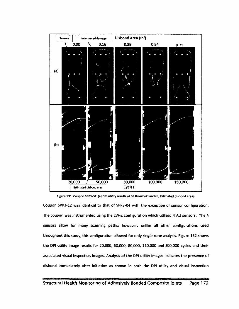
Disbond Area (in2)
0.39
Interpreted damage
80,000 Cycles Estimated disbond area
Figure 131: Coupon SPP3-04: (a) DPI utility results at 05 threshold and (b) Estimated disbond areas
Coupon SPP2-12 was identical to that of SPP3-04 with the exception of sensor configuration.
The coupon was instrumented using the LW-2 configuration which utilized 4 AU sensors. The 4
sensors allow for many scanning paths; however, unlike all other configurations used
throughout this study, this configuration allowed for only single zone analysis. Figure 132 shows
the DPI utility image results for 20,000, 50,000, 80,000, 110,000 and 200,000 cycles and their
associated visual inspection images. Analysis of the DPI utility images indicates the presence of
disbond immediately after initiation as shown in both the DPI utility and visual inspection
Structural Health Monitoring of Adhesively Bonded Composite Joints Page 172
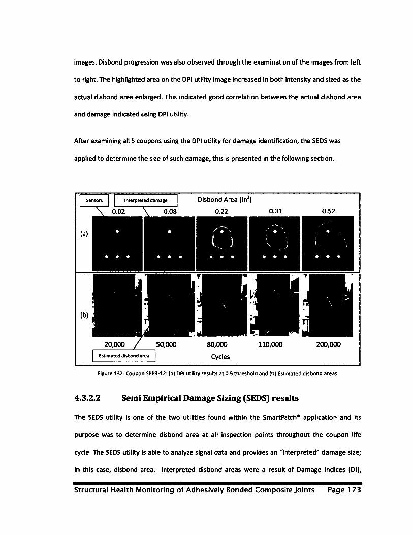
images. Disbond progression was also observed through the examination of the images from left
to right. The highlighted area on the DPI utility image increased in both intensity and sized as the
actual disbond area enlarged. This indicated good correlation between the actual disbond area
and damage indicated using DPI utility.
After examining all 5 coupons using the DPI utility for damage identification, the SEDS was
applied to determine the size of such damage; this is presented in the following section.
Disbond Area (in2)
0.22
Interpreted damage
Estimated disbond area
Figure 132: Coupon SPP3-12: (a) DPI utility results at 0.5 threshold and (b) Estimated disbond areas
4.3.2.2 Semi Empirical Damage Sizing (SEDS) results
The SEDS utility is one of the two utilities found within the SmartPatch* application and its
purpose was to determine disbond area at all inspection points throughout the coupon life
cycle. The SEDS utility is able to analyze signal data and provides an "interpreted" damage size;
in this case, disbond area. Interpreted disbond areas were a result of Damage Indices (Dl),
Structural Health Monitoring of Adhesively Bonded Composite Joints Page 173

which were described in more detail within section 2.2.3.2. Damage Indices are obtained by
creating a Bspace file and by providing known disbond areas for the first few inspections to the
application. For SPP3-03, SPP3-04, SPP3-16, SPP3-4a and SPP3-12 approximately 40% of all
collected signal data was assigned to the Bspace file. Multiple analyses were executed for each
coupon, each with a different number of known disbond area inputs. Coupons SPP3-03, SPP3-04
and SPP3-16 were equipped with LW-1 configuration while SPP3-4a and SPP3-12 were equipped
with LW-2. Results for all coupons utilizing LW-1 sensor configuration were similar and therefore
only one set of results is present below.
Coupon SPP3-04 was equipped with the LW-1 sensor configuration and was analysed under
multiple input conditions using the SEDS utility, each analysis with different known disbond area
inputs. Analyses for the interpretation of disbond area were executed with as little as 12 and as
high as 21 known disbond area inputs. In total, there were 23 signal data files gathered for this
coupon and the SEDS utility analysed all signal data against the Bspace to determine disbond
areas which were not provided to the software. Figure 133 shows disbond area interpretations
for analysis with 12 (60,000 cycle curve), 14 (80,000 cycle curve), 16 (100,000 cycle curve), 18
(120,000 cycle curve) and 21 (150,000 cycle curve) disbond area data point inputs. In addition to
the analysis curves, the actual disbond area curve is also plotted within Figure 133. While
examining each of the curves produced by the SEDS utility within Figure 133, it is evident that
none of the interpretation produced values which are close to that of the actual disbond area.
Increase of the number of disbond area inputs resulted in over-predictions of the disbond area.
The over-interpretation of disbond area was attributed to disbond of both the patch and the
sensors; primarily dominated by sensor disbond.
Structural Health Monitoring of Adhesively Bonded Composite Joints Page 174
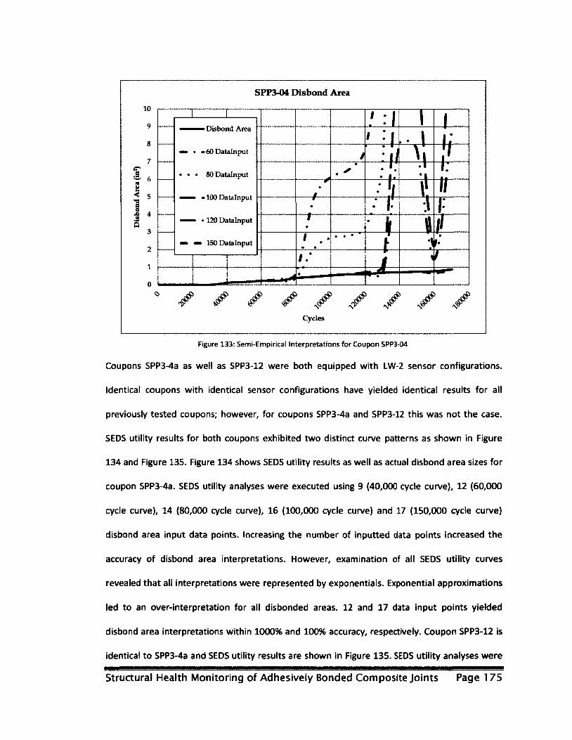
SPP3-04 Disbond Area
10
9 Disbond Area
8 60 Datalnput
7
80 Datalnput 6
5 100 Datalnput
4 120 Datalnput
3 150 Datalnput
2
1
0
Cycles
Figure 133: Semi-Empirical Interpretations for Coupon SPP3-04
Coupons SPP3-4a as well as SPP3-12 were both equipped with LW-2 sensor configurations.
Identical coupons with identical sensor configurations have yielded identical results for all
previously tested coupons; however, for coupons SPP3-4a and SPP3-12 this was not the case.
SEDS utility results for both coupons exhibited two distinct curve patterns as shown in Figure
134 and Figure 135. Figure 134 shows SEDS utility results as well as actual disbond area sizes for
coupon SPP3-4a. SEDS utility analyses were executed using 9 (40,000 cycle curve), 12 (60,000
cycle curve), 14 (80,000 cycle curve), 16 (100,000 cycle curve) and 17 (150,000 cycle curve)
disbond area input data points. Increasing the number of inputted data points increased the
accuracy of disbond area interpretations. However, examination of all SEDS utility curves
revealed that all interpretations were represented by exponentials. Exponential approximations
led to an over-interpretation for all disbonded areas. 12 and 17 data input points yielded
disbond area interpretations within 1000% and 100% accuracy, respectively. Coupon SPP3-12 is
identical to SPP3-4a and SEDS utility results are shown in Figure 135. SEDS utility analyses were
Structural Health Monitoring of Adhesively Bonded Composite Joints Page 175
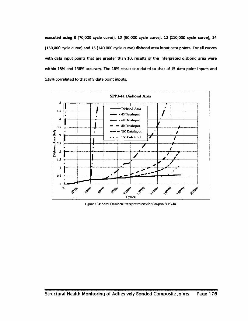
executed using 8 (70,000 cycle curve), 10 (90,000 cycle curve), 12 (110,000 cycle curve), 14
(130,000 cycle curve) and 15 (140,000 cycle curve) disbond area input data points. For all curves
with data input points that are greater than 10, results of the interpreted disbond area were
within 15% and 138% accuracy. The 15% result correlated to that of 15 data point inputs and
138% correlated to that of 9 data point inputs.
SPP3-4a Disbond Area
1 " •
1 1 1 1
••—•Disbond Area
• 40 Datalnput
— • 60 Datalnput
™ • 80 Datalnput
— — — 100 Datalnput
• • • 150 Datalnput
V •
1 •
1 1 1 ••—•Disbond Area
• 40 Datalnput
— • 60 Datalnput
™ • 80 Datalnput
— — — 100 Datalnput
• • • 150 Datalnput
/ 1
1 1 1 ••—•Disbond Area
• 40 Datalnput
— • 60 Datalnput
™ • 80 Datalnput
— — — 100 Datalnput
• • • 150 Datalnput
f t 1 •
1 1 1 ••—•Disbond Area
• 40 Datalnput
— • 60 Datalnput
™ • 80 Datalnput
— — — 100 Datalnput
• • • 150 Datalnput
• /
¥
/
1
1 1 1 ••—•Disbond Area
• 40 Datalnput
— • 60 Datalnput
™ • 80 Datalnput
— — — 100 Datalnput
• • • 150 Datalnput / / 1 1
/ / 1
• / •
f i f
>
1 / / S
'f / /
• • • * s'
t >
*
• t \
\
• •
° ^ / ./ /• / / /
Cycles
Figure 134: Semi-Empirical Interpretations for Coupon SPP3-4a
Structural Health Monitoring of Adhesively Bonded Composite Joints Page 176
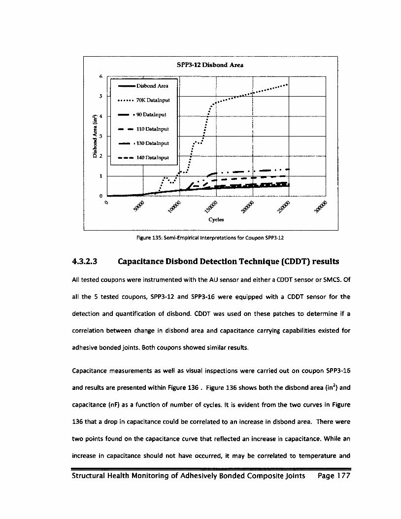
SPP3-12 Disbond Area
6
5
6
5
«—•» Disbond Area • • • *
6
5
•
I4
1' ©
.2 D 2
• 90 Datalnput • • •
I4
1' ©
.2 D 2
— —» 110 Datalnput
• • • • • •
I4
1' ©
.2 D 2
• 130 Datalnput •
• • • •
I4
1' ©
.2 D 2 — -» 140 Datalnput •
•
1 • • • • «—• *
. MM • • "
• • • • • • • \ •
<5
• / ̂ / Cycles
Figure 135: Semi-Empirical Interpretations for Coupon SPP3-12
4.3.2.3 Capacitance Disbond Detection Technique (CDDT) results
All tested coupons were instrumented with the AU sensor and either a CDDT sensor or SMCS. Of
all the 5 tested coupons, SPP3-12 and SPP3-16 were equipped with a CDDT sensor for the
detection and quantification of disbond. CDDT was used on these patches to determine if a
correlation between change in disbond area and capacitance carrying capabilities existed for
adhesive bonded joints. Both coupons showed similar results.
Capacitance measurements as well as visual inspections were carried out on coupon SPP3-16
and results are presented within Figure 136 . Figure 136 shows both the disbond area (in2) and
capacitance (nF) as a function of number of cycles. It is evident from the two curves in Figure
136 that a drop in capacitance could be correlated to an increase in disbond area. There were
two points found on the capacitance curve that reflected an increase in capacitance. While an
increase in capacitance should not have occurred, it may be correlated to temperature and
Structural Health Monitoring of Adhesively Bonded Composite Joints Page 177
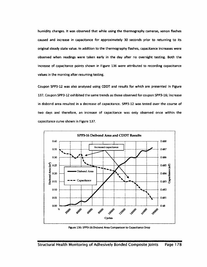
humidity changes. It was observed that while using the thermography cameras, xenon flashes
caused and increase in capacitance for approximately 30 seconds prior to returning to its
original steady state value. In addition to the thermography flashes, capacitance increases were
observed when readings were taken early in the day after no overnight testing. Both the
increase of capacitance points shown in Figure 136 were attributed to recording capacitance
values in the morning after resuming testing.
Coupon SPP3-12 was also analysed using CDDT and results for which are presented in Figure
137. Coupon SPP3-12 exhibited the same trends as those observed for coupon SPP3-16; increase
in disbond area resulted in a decrease of capacitance. SPP3-12 was tested over the course of
two days and therefore, an increase of capacitance was only observed once within the
capacitance curve shown in Figure 137.
SPP3-16 Dsibond Area and CDDT Results
0.40 0.488
Increased capacitance 0.487 0.35
0.486 0.30
0.485 E" .5 0.25
Disbond Area 0.484
0.483 <3 Capacitance
0.482 0.10
0.05 0.481
0.00 0.48
Cycles
Figure 136: SPP3-16 Disbond Area Comparison to Capacitance Drop
Structural Health Monitoring of Adhesively Bonded Composite Joints Page 1 78
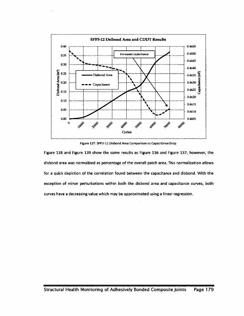
SPP3-12 Dsibond Area and CDDT Results
0.40
0.35
0.30
1.0.25 <9 I < 0.20 t3
6 O « 0.15 Q
0.10
0.05
0.00
\
| |
\ Increased capacitance X
X N
Increased capacitance X
X N
Disbond Area
— — — Capacitance
Disbond Area
— — — Capacitance
> \ \ \
Disbond Area
— — — Capacitance \ >
\
\ >
\ \
\ \ \ \ *
V"" %
0.4655
0.4650
0.4645
0.4640
0.4635 f V U
0.4630 S3 V
0.4625 U
0.4620
0.4615
0.4610
0.4605
^ ^ ^ ^ Cycles
Figure 137: SPP3-12 Disbond Area Comparison to Capacitance Drop
Figure 138 and Figure 139 show the same results as Figure 136 and Figure 137; however, the
disbond area was normalized as percentage of the overall patch area. This normalization allows
for a quick depiction of the correlation found between the capacitance and disbond. With the
exception of minor perturbations within both the disbond area and capacitance curves, both
curves have a decreasing value which may be approximated using a linear regression.
Structural Health Monitoring of Adhesively Bonded Composite Joints Page 179
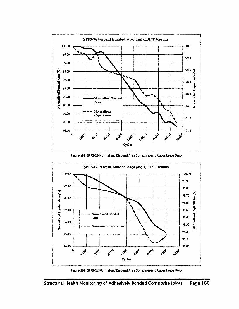
SPP3-16 Percent Bonded Area and CDDT Results
100.00
99.50
99.00
98.50
98.00
97.50
97.00
96.50
96.00
95.50
95.00
\ J
V 1' ' X ' * \ 1 1 \ \
V"5 \ %
V \
k \ \ * ^» Normalized Bonded
Area
Normalized Capacitance
\ k \ \ *
^» Normalized Bonded Area
Normalized Capacitance
> \
^» Normalized Bonded Area
Normalized Capacitance
\
k.
^» Normalized Bonded Area
Normalized Capacitance \
\ > \
\ \
> \
100
99.8
99.6 3" V U 1
99.4
U 99.2 1
X
99 Z
98.8
98.6
V Cycles
/ / /
Figure 138: SPP3-16 Normalized Disbond Area Comparison to Capacitance Drop
SPP3-12 Percent Bonded Area and CDDT Results
100.00
99.00
a 98.00 •3
•8 § 97.00 A •O £ 2 96.00 s o Z
95.00
94.00
\ > \
%
Nv \ > \ \
Normolized Bonded Area
— — — Normalized Capacitance
\ % \ \
Normolized Bonded Area
— — — Normalized Capacitance
r~
* \ \ J?
100.00
- 99.90
99.80
99.70 V
99.60 I rt
99.50
99.40 | e
99.30
99.20
99.10
99.00
o Z
Cycles
Figure 139: SPP3-12 Normalized Disbond Area Comparison to Capacitance Drop
Structural Health Monitoring of Adhesively Bonded Composite Joints Page 180

Based on the above results, this SHM technique provides value in the quantification of damage.
Equations may be developed to model the change in capacitance with respect to disbond;
however, these equations will be only applicable to this patch configuration. Changes in patch
shape, temperature, humidity and ultra violet are amongst parameters that will both influence
the equations as well as the reliability of this system.
4.3.2.4 Surface Mountable Crack Detection System (SMCDS) results
All tested coupons were instrumented with AU sensors and either a CDDT or SMCS. Of all the 5
tested coupons, SPP3-03, SPP3-04 and SPP3-4a were equipped with SMCS for the detection of
disbond. Unlike both the AU and the CDDT SHM systems, SMCS does not quantify the disbond
area size rather it indicates when cracks along the edge of the patch have reached a certain
point. SMCS were only placed along strategic locations around the tip of the patch as shown in
Figure 140. As cracks within the adhesive grew alongside the patch, certain SMCS were triggered
(i.e. the circuit was broken). Analysis for all coupons instrumented using the SMCDS technique
resulted in the same conclusions and therefore only results for one coupon are presented.
Coupon SPP3-04 was equipped with the SMCS as shown in both Figure 140 and Figure 141.
Three SMCS were placed approximately 0.15 inches apart as shown in Figure 140 magnification
A. During fatigue, cracks initiated within the adhesive, at the tip of the patch and propagated
through the SMCS as shown in Figure 141. Crack growth through the SMCS resulted in an open
electrical circuit during applied load and closed circuit during no load. It was also difficult to
visually inspect SMCS cracking with no applied load as the circuit was closed and the SMCS is
very reflective under lighting as shown in Figure 141. For that reason, the circuit was
interrogated during fatigue, and upon the first open circuit indication, the circuit was assumed
broken regardless of its future open/closed positions. At later stages within the lifecycle of the
Structural Health Monitoring of Adhesively Bonded Composite Joints Page 181
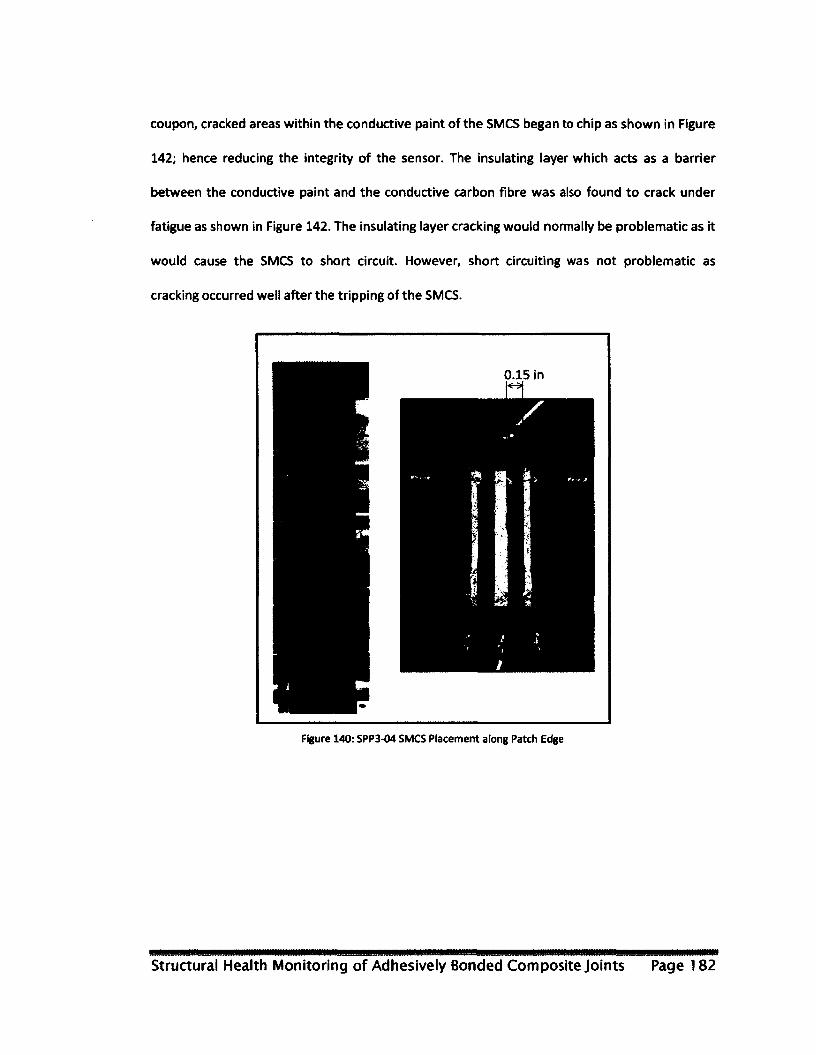
coupon, cracked areas within the conductive paint of the SMCS began to chip as shown in Figure
142; hence reducing the integrity of the sensor. The insulating layer which acts as a barrier
between the conductive paint and the conductive carbon fibre was also found to crack under
fatigue as shown in Figure 142. The insulating layer cracking would normally be problematic as it
would cause the SMCS to short circuit. However, short circuiting was not problematic as
cracking occurred well after the tripping of the SMCS.
Figure 140: SPP3-04 SMCS Placement along Patch Edge
Structural Health Monitoring of Adhesively Bonded Composite Joints Page 182
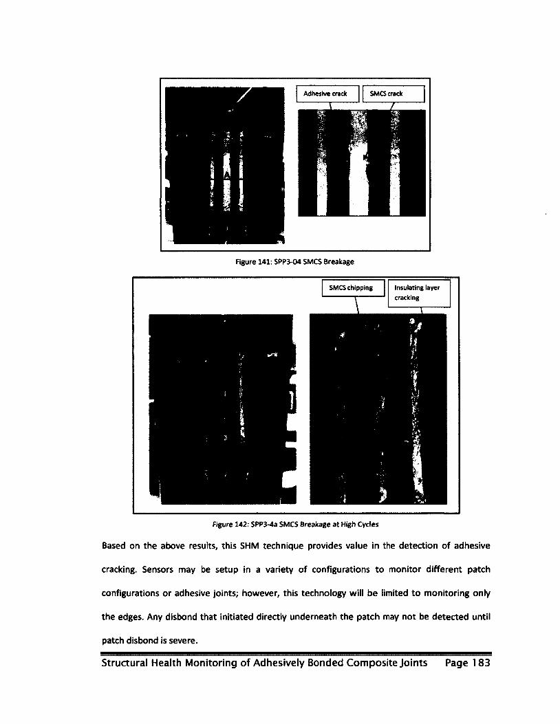
Adhesive crack SMCS crack
Figure 141: SPP3-04 SMCS Breakage
SMCS chipping Insulating layer
cracking
Figure 142: SPP3-4a SMCS Breakage at High Cycles
Based on the above results, this SHM technique provides value in the detection of adhesive
cracking. Sensors may be setup in a variety of configurations to monitor different patch
configurations or adhesive joints; however, this technology will be limited to monitoring only
the edges. Any disbond that initiated directly underneath the patch may not be detected until
patch disbond is severe.
Structural Health Monitoring of Adhesively Bonded Composite Joints Page 183

Chapter 5.0: Conclusions
This thesis focused ori the use of Structural Health Monitoring (SHM) Systems for the detection
and quantification of crack and disbond growth. Three SHM systems were tested within this
research: Acousto-Ultrasonic (AU), Capacitance Disbond Detection Technique (CDDT) and
Surface Mountable Crack Detection System (SMCDS). The AU system used within this research
was manufactured by Acellent Technologies Inc. AU is a process in which Lamb Waves (LW) are
transmitted through a structure and analysed for the detection and quantification of damage.
Changes between current signals and benchmark signals indicate damage formation. The CDDT
technology used within this research is a process that has been tested at the National Research
Council Canada (NRC) for the detection of disbond. CDDT is a process in which patch adhesion
may be quantified by its ability to carry a capacitive charge. Disbond of a patch from a substrate
results in a change in capacitance, which may be correlated to the damage size. SMCDS
technology is a process in which conductive paint is placed onto a surface which is subjected to
cracking. Cracking within the component surface also propagates through the conductive paint,
which results into a failed sensor. A failed sensor is detected by its inability to conduct current
while under interrogation.
To test these three SHM suites for the detection of crack and disbond growth, three coupon sets
were designed. The first set of coupons was made of aluminum and had a center surface crack;
these coupons were used for the evaluation of the SHM systems for their effectiveness in crack
growth detection. The second set of coupons was made of an aluminum substrate and a carbon
fibre patch. Both the patch and the substrate were bonded together; these coupons were for
the evaluation of the SHM systems for their effectiveness in crack and disbond growth
detection. The third set of coupons was made of a carbon fibre substrate and a boron fibre
patch. Both the patch and the substrate were bonded together; these coupons were for the
Structural Health Monitoring of Adhesively Bonded Composite Joints Page 184

evaluation of the SHM systems for their effectiveness in disbond growth detection. All coupons
were designed through the aid of Finite Element Analysis. The designed coupons were
manufactured and instrumented with SHM sensors at NRC. AU, CDDT and SMCDS were all
instrumented on the coupons. Coupons where split in two groups; SMCDS were installed on one
and CDDT sensors on the other. However, all coupons were instrumented with AU sensors.
Results of crack growth monitoring using the AU system for coupon Set 1 was analyzed using the
DPI and the SEDS utilities. Multiple coupons were tested using this system and analyzed using
the two utilities. The DPI utility was able to indicate the initiation as well as propagation of
cracks on all tested coupons. In some cases, the DPI utility provided damage identification in the
correct location of the crack while in other cases, the identified location was found just below
the actual crack. The SEDS utility was also used to interpret crack lengths. For all tested coupons,
the results were conservative when compared to the actual crack lengths. These results were
based on polynomial approximations using DIs. In some cases, the crack length interpretations
contained an interpretation spike within the data. This spike is an outlier which is an over-
interpreted crack length. If discarded, the crack length interpretations yielded an exponential
crack growth graph similar to that of the actual measured crack length. On some coupons, crack
interpretation spikes occurred more than once within the same data set.
Analysing disbond using the AU system on composite patches adhesively joined to an aluminum
substrate was also carried out using both the DPI and SEDS utilities. Multiple sensor
configurations were used on multiple coupons. Variances within sensor configurations were
utilized to determine if greater scanning accuracy and resolution may be obtained. Through the
use of many sensors, damage detection analysis was isolated to specific zones along the coupon.
This was done to monitor disbond at the tip, the center and the base of the patch. Based on
Structural Health Monitoring of Adhesively Bonded Composite Joints Page 185

multi-zone (simultaneous zone) analysis, the DPI indicated major disbond along the entire patch;
this however was inaccurate when compared to the Non-Destructive Evaluation (NDE) results.
The analysis of single zones did result in greater accuracy as compared to the analysis of all
zones simultaneously. In cases where only the tip of the patch was examined, NDE results
correlated with the DPI results. However, it was found that results for the bottom of the patch
were not always accurate. In some cases, the DPI utility indicated disbond where no disbond
existed and in other cases it indicated disbond where disbond existed. SEDS utility was also
applied to analyze all the coupons and each analysis provided different results. In some cases,
disbond size was over-interpreted by a maximum of 375% and in other cases by a minimum of
45%. All coupons were identical; however, results were very different for each coupon. In
addition to over-prediction of disbond size, some interpretations resulted in an under-
interpretation. Under-interpreted disbond areas are dangerous as they provide false
information regarding the integrity of the bond.
Monitoring of disbond on composite patches adhesively joined to a composite substrate was
done through the use of the AU, CDDT and SMCDS SHM systems. The DPI and the SEDS utilities
were used to analyse the disbond area location and size. For these coupons, two sensor layouts
were used. For the sensor layout that contained sensors bonded to the substrate and the patch,
it was found that the sensors experienced disbond from the substrate as a result of high strain.
Sensor configurations which only contained sensors on the patch did not experience sensor
disbond. The DPI utility was used to analyze results for both sensor layouts. For the layout which
had sensors on the substrate, the DPI utility indicated damage in all areas of the patch. This was
inaccurate when compared to the NDE results. These results were attributed to poor signal
transmission which was a result of sensor disbond. Coupons with sensors only on the substrate
provided better results than those which experienced sensor disbond. In all cases, the DPI utility
Structural Health Monitoring of Adhesively Bonded Composite Joints Page 186
provided damage location and progression identification that was closely correlated to those
found using NDE. SEDS utility was also used to analyze the data of all the coupons. For coupons
with sensors on the substrate, the disbond area interpretation provided results which were in
no way comparable to the actual disbond area. For coupons which had no sensors on the
substrate, disbond area interpretations were conservative when compared to the actual
disbond areas. In some cases, disbond size was over-interpreted by a maximum of 138% and in
other cases by a minimum of 15%. None of the disbond area interpretations were found to be
less than the actual disbond area. CDDT and SMCDS were also implemented to monitor disbond
on these patches. In CDDT, capacitance drop was observed as the patch disbond area increased.
CDDT results indicated that disbond area may be correlated to change within capacitance and
that the trend may be linear. CDDT was found to be useful for the quantification of patch
disbond; however, was not useful for the indication of disbond location. The SMCDS was also
used and found to indicate where and when the adhesive edges along the patch began to crack.
Both the CDDT and the SMCDS techniques could be used together to indicate damage location
and size when implemented properly on specific geometries.
Structural Health Monitoring of Adhesively Bonded Composite Joints Page 187
References
[1] G Wheatley, J Kollgaard, J Register, and M Zaidi, "Comparative Vacuum Monitoring as an
Alternate Means of Compliance," in Structural Health Monitoring, 2003, pp. 1358-1365.
{2] V. Giurgiutiu, Structural health monitoring with piezoelectric wafer active sensors. Boston,
USA: Academic Press, 2008.
[3] David Roylance, Introduction to Composite Materials. Massachusetts Institute of
Technology, Cambridge, USA, March 20, 2000.
[4] Daniel B Miracle and Steven L Donaldson, Introduction to Composites. Air Force Research
Laboratory, United States.
[5] Kutz and Mayer, Handbook of Material Selection. New York, USA: John Wiley & Sons, 2002.
[6] G.B.Murri, "Testing and life predictions of composite materials," U.S. Army Research
Laboratory, Vehicle Technology Directorate, Hampton, March 23,2006.
[7] United States Dept. of Defense, Composite materials handbook. Material usage, design and
analysis. Washington, D.C, United States: United States Dept. of Defense, 2002.
[8] A. A. Baker, S. Dutton, and D. Kelly, Composite Materials for Aircraft Structures, secon
edition ed.: American Institute of Aeronautics and Astronautics, 2004.
[9] Daniel Feszty, "Rotorcraft," Carleton University, Ottawa, Class Lecture 2009.
[10] Sanjay k Mazumdar, Composite manufacturing: product, and process engineering. Dallas,
Texsas: CRC press, 2001.
[11] Ravi B Deo, James H Starnes, and Richard C Holzwarth, "Low-Cost Composite Materials and
Structures for Aircraft Applications," in RTO-MP-069(II), Loen, 2001.
[12] Boeing, "Commercial Airplanes - 787 Dreamliner - Background," Boeing, Seattle, Press
release 2010.
[13] Richard A Leyes and William Fleming, The History of North American Small Gas Turbine
Aircraft Engines, illustrated ed. USA: AIAA, 1999.
[14] Driver Side. (2009, Spetember) Aston Martin Showes off Some of the One-77 at Geneva.
[Online], http://www.driverside.com/backseatdriver/2009/03/04/aston-martin-shows-off-
some-of-the-one-77-at-geneva/comments-page-l/
Structural Health Monitoring of Adhesively Bonded Composite Joints Page 188

[15] Auto Blog. (2009, Sepetember) Aston Martin One-77 Uncovered: In-depth on what's under
the skin. [Online], http://www.autoblog.com/2009/03/06/aston-martin-one-77-uncovered-
in-deoth-on-whats-under-the-skin/
[16] David A Nethercot, Composite Construction. New York, USA: Spon Press, 2003.
[17] C Zweben, Composite Materials and Mechanical Design, Mechanical Engineer's Handbook,
2nd ed. New York, USA: John Wiley & Sons, 1998.
[18] F L Matthews, Joining Fibre-Reinforced Plastics. New York, USA: Elsevier Applied Science,
1987.
[19] R Martin, Ageing of Composites. Cambridge, England: Woodhead Punlishing Limited, 2008.
[20] M D Bannea and L F M da Silvia, "Adhesively Bonded Joints in Composite Matrerial: an
Overview," Insituti de Engenharia Mecanica, Porto, Portugal, 2008.
[21] Keith B. Armstrong, L. Graham Bevan, and William F. Cole, Care and Repair of Advanced
Composites, 2nd ed.: Society of Automotive Engineers, Inc., 2005.
[22] A.A. Baker, RJ. Callinan, M J. Davis, R Jones, and J.G. Williams, "Repair of mirage III aircraft
using the BFRP crack-patching technique," Theoretical and Applied Fracture Mechanics 2,
pp. 1-15,1984.
[23] A.A. Baker, "Repair of cracked or defective metallic aircraft components with advanced
fibre composites," Composite Structures 2, pp. 153-181,1984.
[24] Satya N Atluri, Structural Integrity and Durability. Forsyth, Georgia, USA: Tech Science Press,
1997.
[25] W Baker, I Mackenzie, and R Jones, "Development of life extension strategies for Australian
military aircrafts, using structural health monitoring of composite repairs and joints,"
Composite Structures, vol. 66, no. 1-4, pp. 133-143, October 2004.
[26] Pierre Noel Marty, N Desai, and J Anderson, "NDT OF KISSING BOND IN AERONAUTICAL
STRUCTURES," in WCNDT, Linkoping, Sweeden, 2004.
[27] Sameer Homoush, Kunigal Shivakumar, Feras Darwish, Mathew Sharpe, and Paul Swindell,
"Defective Repairs of Laminated Solid Composites," Journal of Composite Materials, vol.
39, no. 24, pp. 2185-2196, Nov 2005.
[28] Mark Lin, Xinlin Qing, Amrita Kumar, and Shawn J Beard, "Smart Layer and Smart Suitcase
for Structural Health Monitoring Applications," in SPIE, Arlington, VA, 22204, 2001, pp. 98-
Structural Health Monitoring of Adhesively Bonded Composite Joints Page 189

106.
[29] M Martinez et al., "Demonstration of an Instrumented Patch Phase 1," National Research
Council Canada, Ottawa, Lab Technical Report LTR-SMPL-2006-0226, 2007.
[30] H. Speckmann and R. Henrich. (2009, June) Structural Health Monitoring (SHM) - Overview
on Technologies underdevelopment. [Online].
http://www.ndt.net/article/wcndt2004/pdf/aerospace/563 henrich.pdf
[31] H. Speckmann, "Structural Health Monitoring (SHM)," IMRBPB Meeting, EASA, Colonge,
Presentation 2007.
[32] W. Staszewski, C. Boiler, and G. Tomlinson, Health monitoring of aerospace structures:
smart sensor technologies and signal processing. Hoboken, NJ, USA: J. Wiley, 2004.
[33] Su Zhongqing and Lin Ye, Identification of damage using Lamb waves from fundamentals to
applications. New York, USA: Springer, 2009.
[34] M Genest, M Martinez, N Mrad, G Renaud, and A Fahr, "Pulsed thermography for non
destructive evaluation and damage growth monitoring of bonded repairs," Composite
Structures, vol. 88, no. 1, pp. 112-120, March 2009.
[35] Holger Speckmann and Henrik Roesner, "Structural Health Monitoring: A Contribution to
the Intelligent Aircraft Structure," in ECNDT, 2006.
[36] Sjostrom F. (2008, December) The ABCs of Fiber Bragg Gratings. [Online].
httP://electronicdesien.com/articles/print.cfm?AD=l&ArticllD=20252
[37] Ail About Circuits. (2009, August) Strain Gauges. [Online].
http://www.allaboutcircuits.com/vol 1/chpt 9/7.html
[38] National Instruments. (2009, June) Measuring Strains with Strain Gauges. [Online].
http://zone.ni.eom/devzone/cda/tut/p/id/3642
[39] M Martinez et al., "Demonstration of an Instrumented Patch - Phase II," National Research
Council Canada, Ottawa, Lab Technical Report LTR-SMPL-2008-0135, 2008.
[40] EADS. (2009, August) Structural Health Monitoring. [Online].
http://www.edas.com/1024/en/madebveads/endurance/shm.html
[41] M Martinez et al., "Surface Mountable Crack Detection System," National Research Council
Canada, Ottawa, LM-SMPL-2009-0037, 2009.
Structural Health Monitoring of Adhesively Bonded Composite Joints Page 190

[42] Acellent Technologies Inc. (2010) Software - SmartPatch. [Online].
http://www.acellentsensors.com/Software SmartPatch.asp
[43] M. Scheerer, "SHM of Composite Structures using Acoustic Emission Methods," in European
Ground Testing Instrumentation Aerospace Testing Expo, Munich, April 15-16, 2008.
[44] Shin-etsu Fujimoto and Hideki Sekine, "Identification of crack and disbond fronts in repaired
aircraft structural panels with bonded FRP composite patches," Composite Structures, vol.
77, no. 4, pp. 533-545, February 2007.
[45] R Jones and RJ Callinan, "A design Study in Crack Patching," Fibre Science and Technology,
vol. 14, no. 2, pp. 99-111, February 1981.
[46] D Quinas, B.B. Bouiadjra, B Serier, and M SaidBekkouche, "Comparison of the effectiveness
of boron/epoxy and graphite/epoxy patches for repaired cracks emanating from a
semicircular notch edge," Composite Structures, vol. 80, no. 4, pp. 514-522, October 2007.
[47] Chorong-Fuh Liu, Horng-Shian Jou, and Ying-Te Lee, "Stress Intensity Factor of Patched
Crack," International Journal of Solids and Structures, vol. 24, no. 13, pp. 1557-1562, May
1997.
[48] M Martinez, G Renaud, D Backman, M Genest, and M Delanny, "Demonstration of an
instrumented patch," in SPIE, 2007, pp. 65300M-1 TO 65300M-11.
[49] Stephen C Galea et al., "Development of Structural Health Monitoring Systems for
Composite Bonded Repairs on Aircraft Structures," in SPIE, 2001.
[50] H Sohn, D Dutta, and Y.K An, "Baseline-Free Damage Detection through Mode Separation of
Lamb Waves using Self-Sensing Piezoelectric Transducers," in Structural Health Monitoring,
2009.
[51] Kelah Wakha, Paul Samuel, and Darryll Pines, "A smart composite patch for the repair of
aircraft structures," in SPIE, Bellingham, 2005.
[52] M Martinez, L Gang, D Backman, A Oudovikine, and N Bellinger, "Crack detection on
composite and metallic aerospace structures," in 4th European Workshop on Structural
Health Monitoring, 2008, pp. 560-569.
[53] Gary L. and Kishoni, Doron Workman, Nondestructive Testing Handbook, Ultrasonic Testing,
3rd ed.: ASNT, 2007.
[54] Clemente Ibarra Castanedo, "Quantitative subsurface defect evaluation by pulsed phase
thermography: depth retrieval with the phase," Faculte des Sciences et de Genie Universite,
Structural Health Monitoring of Adhesively Bonded Composite Joints Page 191

Laval, Ph.D Thesis 2005.
[55] X Maldague, F Galmiche, and A Ziadi, "Advances in Pulsed Phase Thermography," Electrical
and Computing Engineering Dept, University Laval, Quebec City, 2001.
[56] X Maldague and S Marinetti, "Pulse Phase Infrared Thermography," Electrical and
Computing Engineering Dept. University Laval, Quebec City, 2001.
[57] Alan Baker, "Structural Health Monitoring of a Bonded Composiite Patch Repair on a
Fatigue-Cracked Wing," Deffence Seience and Technology Organisation Victoria, Victoria,
Australia, DTSO-RR-0335,2008.
[58] William Hart Hayt, Jack Ellsworth Kemmerl, and Steven M Durbin, Engineering circuit
analysis, 7th ed. New York, USA: McGraw-Hill Higher Education, 2001.
[59] Larry K Baxter, Capacitive Sensors: Design and Applications. New York, USA: IEEE Press,
1997.
[60] J. Stevan, Damage Detection Using Lamb Waves for Structural Health Monitoring. USA: Air
Force Institute Of Technology, 2007.
[61] V Giurgiutiu and A Cue, "Concepts for using Piezoelectric Wafer Active Sensors in Rotorcraft
Health Monitoring," in Structural Health Monitoring, 2005, pp. 1173-1182.
[62] A A Baker, Nick Rajic, and Claire Davis, "Towards a practical structural health monitoring
technology for patched cracks in aircraft structure," Composites Part A: Applied Science and
Manufacturing, vol. 40, no. 9, pp. 1340-1352, Sepetember 2009.
[63] Gareth S Pierce, Brian Culshaw, Graeme Manson, Keith Worden, and Wieslaw Staszewski,
"Application of ultrasonic Lamb wave techniques to the evaluation of advanced composite
structures," in SPIE, 2000, pp. 93-103.
[64] Shashank Pant, "Damage Detection Using Lamb Waves: Derivation of Lamb Wave Equations
for Structural Health Monitoring (SHM) Applications," Carleton University, Ottawa, 2010.
[65] Joseph L Rose, Ultrasonic Waves in Solid Media, 1st ed. Cambridge, England: Cambridge
University Press, 2004.
[66] Sourav Banerjee, Shawn Beard, Fady Habib, and Marcias Martinez, "Damage Quantification
using Smart Patch System for Hot Spot," in SPIE, 2010.
[67] Preformance Composites Ltd. (2009, July) Mechanical Properties of Carbon Fibre Composite
Materials, Fibre / Epoxy resin (120°C Cure). [Online]. http://www.performance-
Structural Health Monitoring of Adhesively Bonded Composite Joints Page 192

composites.com/carbonfibre/mechanicalDroperties 2.asp
[68] Cytec Engineered Materials. (2010) Cytec, CYCOM 5276-1. [Online].
https://www.cvtec.com/engineered-materials/products/Datasheets/CYCQM%205276-l.pdf
[69] Specialty Materials, Inc. (2010) Specialty Materials, Boron PrepregTape Properties.
[Online], http://www.specmaterials.com/boronprepregproperties.htm
[70] Cytec Engineered Materials. (2011) FM 73 Epoxy Film Adheisive. [Online].
http://www.cvtec.com/engineered-materials/products/Datasheets/FM73-081111.pdf
Structural Health Monitoring of Adhesively Bonded Composite Joints Page 193