STRUCTURAL DESIGN, ANALYSIS AND COMPOSITE …etd.lib.metu.edu.tr/upload/12610575/index.pdf ·...

LOW VELOCITY IMPACT ANALYSIS OF A COMPOSITE MINI UNMANNED AIR VEHICLE DURING BELLY LANDING

A THESIS SUBMITTED TO THE GRADUATE SCHOOL OF NATURAL AND APPLIED SCIENCES

OF MIDDLE EAST TECHNICAL UNIVERSITY

BY

SERHAN YÜKSEL

IN PARTIAL FULFILLMENT OF THE REQUIREMENTS FOR

THE DEGREE OF MASTER OF SCIENCE IN

AEROSPACE ENGINEERING

MAY 2009

Approval of the thesis:

LOW VELOCITY IMPACT ANALYSIS OF A COMPOSITE MINI UNMANNED AIR VEHICLE DURING BELLY LANDING

submitted by SERHAN YÜKSEL in partial fulfillment of the requirements for the degree of Master of Science in Aerospace Engineering Department, Middle East Technical University by, Prof. Dr. Canan Özgen __________________ Dean, Graduate School of Natural and Applied Sciences Prof. Dr. Ġsmail Hakkı Tuncer __________________ Head of Department, Aerospace Engineering Assoc. Prof. Dr. Altan Kayran __________________ Supervisor, Aerospace Engineering Dept., METU

Examining Committee Members: Prof. Dr. Nafiz ALEMDAROĞLU __________________ Aerospace Engineering Dept., METU Assoc. Prof. Dr. Altan KAYRAN __________________ Aerospace Engineering Dept., METU Asst. Prof. Dr. Melin ġAHĠN __________________ Aerospace Engineering Dept., METU Asst. Prof. Dr. Güçlü SEBER __________________ Aerospace Engineering Dept., METU Asst. Prof. Dr. Ferhat AKGÜL __________________ Engineering Sciences, METU

Date: __________________

iii

I hereby declare that all information in this document has been obtained and presented in accordance with academic rules and ethical conduct. I also declare that, as required by these rules and conduct, I have fully cited and referenced all material and results that are not original to this work. Name, Last Name : Serhan YÜKSEL

Signature :

iv

ABSTRACT

LOW VELOCITY IMPACT ANALYSIS OF A COMPOSITE MINI UNMANNED AIR

VEHICLE DURING BELLY LANDING

Yüksel, Serhan

M.Sc., Department of Aerospace Engineering

Supervisor: Assoc. Prof. Dr. Altan KAYRAN

May 2009, 118 pages

Mini Unmanned Aerial Vehicles (UAV) have high significance among other UAV’s, in

different categories, due to their ease of production, flexibility of maintenance,

decrease in weight due to the elimination of landing gear system and simplicity of

use. They are usually built to meet “hand launching” and “belly landing” criteria in

order to have easy flight and easy landing features. Due to the hand take-off and

belly landing features there is no need to have a runway and this feature is a very

significant advantage in operational use.

In an operation belly landing mini UAV’s may encounter tough landing areas like

gravel, concrete or hard soil. Such landing areas may create landing loads which

are impulsive in character. The effect of the landing loads on the airframe of the mini

unmanned air vehicle must be completely understood and the mini UAV be

designed accordingly in order not to damage the mini UAV during belly landing.

Typical impact speeds during belly landing is relatively low (<10 m/s) and in general

belly landing phenomenon can be treated as low velocity impact.

v

The purpose of this study is to analyze the impact loads on the composite sub-

structures of a mini UAV due to the belly landing. “Güventürk” Mini UAV, which is

designed and built in METU Aerospace Engineering Department, is used as the

analysis platform. This study is limited to the calculation of stresses and deformation

that is caused by the low velocity impact forces encountered during belly landing.

The main purpose of this work is to help the designer in making design decisions for

a mini UAV that is tolerable to low velocity impact loads.

Initial part of the thesis includes analytical treatment of low velocity impact

phenomenon. In the simplified analytical approach the loading is assumed as quasi-

static and comparisons of such a simplified method of analysis is made with explicit

finite element solutions on isotropic and composite plate structures to investigate the

applicability of simplified analytical method of analysis.

Belly landing analyses of the mini UAV are done by MSC.Dytran, which is an explicit

finite element solver. Model building and post processing are done via MSC.Patran.

Stress and deformation response of the mini UAV is investigated by performing low

velocity impact analysis using sub-structure built-up approach.

Keywords: Unmanned air vehicle, low velocity impact, belly landing, composite

structure

vi

ÖZ

LOW VELOCITY IMPACT ANALYSIS OF A COMPOSITE MINI UNMANNED AIR

VEHICLE DURING BELLY LANDING

Yüksel, Serhan

Yüksek Lisans, Havacılık ve Uzay Mühendisliği Bölümü

Tez Yöneticisi: Doç. Dr. Altan KAYRAN

Mayıs 2009, 118 sayfa

Mini Ġnsansız Hava Araçları (ĠHA) üretim kolaylığı, bakım esnekliği, iniĢ takımları

olmadığı için düĢük ağırlığı ve kullanım kolaylığı dikkate alındığında diğer ĠHA’lar

arasında önemli bir yere sahiptir. Kolay uçuĢ ve kolay iniĢ özelliklerine sahip

olmaları için genellikle elden atılıp gövde üstüne inerler. Elden atılıp gövde üstüne

iniĢ yaptıkları için piste ihtiyaç duymamaları operasyonel kullanımları göz önünde

bulundurulduğunda büyük bir avantajdır.

Operasyonel kullanımda gövde üstüne iniĢ yapan ĠHA’lar çakıl, beton ve sert toprak

gibi zorlu iniĢ alanları ile karĢılaĢabilirler. Bu tip alanlar çok yüksek iniĢ yüklerini

ortaya çıkarırlar. Gövde üstü iniĢ sırasında ĠHA’nın iskelet yapısına hasar vermemek

için bu yükler tamamen anlaĢılmalı ve mini ĠHA bu yüklere göre tasarlanmalıdır.

Gövde üstü iniĢlerde çarpıĢma hızı genellikle düĢüktür (<10 m/s) ve düĢük hızda

darbe kapsamında değerlendirilebilir.

Bu tezin amacı gövde üstü iniĢ esnasında bir mini ĠHA’nın kompozit parçaları

üzerine binen yüklerin analizidir. Analizlerde ODTÜ Havacılık ve Uzay Mühendisliği

vii

bölümünde tasarlanıp üretilen Güventürk Mini ĠHA kullanılmıĢtır. Bu tez gövde üstü

iniĢ sırasında ortaya çıkan gerilim ve deformasyonun hesaplanması ile sınırlıdır.

Tezin temel amacı tasarımcıya düĢük hızlı çarpıĢma yüklerine dayanıklı bir mini ĠHA

yapılmasında karar vermesine yardımcı olmaktır.

Tezin ilk bölümü düĢük hızlı çarpıĢmanın analitik uygulamasını içermektedir.

BasitleĢtirilmiĢ analitik yaklaĢımda yükleme “neredeyse statik” kabul edilmiĢ ve elde

edilen çözümler izotropik ve kompozit plakalar üzerinde uygulanan “açık-ekspilisit”

sonlu eleman çözümü ile karĢılaĢtırılarak basitleĢtirilmiĢ analitik yaklaĢımın

uygulanabilirliği incelenmiĢtir.

DüĢük hızda çarpıĢma analizlerinde “açık-ekspilisit” sonlu elemanlar kodu olan

MSC.Dytran kullanılmıĢtır. Modelleme ve sonuçların analizi için MSC.Patran

kullanılmıĢtır. Mini ĠHA’nın stres ve deformasyon tepkileri alt elemanların birleĢimi

yaklaĢımı ile incelenmiĢtir.

Anahtar Kelimeler: Ġnsansız hava aracı, düĢük hızda çarpıĢma, gövde üstü iniĢ,

kompozit yapı

viii

to my family…

ix

ACKNOWLEDGEMENTS

I would like to express the deepest gratitude for Assoc. Prof. Dr. Altan Kayran

whose invaluable efforts and support guided me throughout my thesis. His friendly

approach together with his encouragement is simply what one could wish from a

supervisor. I am also thankful to Prof. Dr. Nafiz Alemdaroğlu, supervisor of METU

UAV Project for the financial and facility support he provided.

Many thanks to my colleagues at METU Aerospace Engineering UAV Laboratory:

Fikri Akçalı, Sercan Soysal, Volkan Kargın and Hüseyin Yiğitler. I also thank to

Murat Ceylan for his work during the manufacturing process of the UAV composite

parts.

Finally, never enough thanks to my family for their trust.

x

TABLE OF CONTENTS

ABSTRACT ............................................................................................................. iv

ÖZ ........................................................................................................................... vi

ACKNOWLEDGEMENTS ........................................................................................ ix

TABLE OF CONTENTS ............................................................................................ x

LIST OF FIGURES ................................................................................................ xvi

LIST OF NOMENCLATURES ............................................................................... xxii

1. INTRODUCTION AND LITERATURE REVIEW ................................................... 1

1.1. Introduction to Unmanned Aerial Vehicles ................................................ 1

1.2. Classification of Unmanned Aerial Vehicles .............................................. 1

1.3. METU “Güventürk” Mini Unmanned Aerial Vehicle ................................... 3

1.4. Impact Phenomenon ................................................................................ 4

1.5. Composite Materials ................................................................................. 6

1.6. Belly Landing UAV’s ................................................................................. 7

1.7. Objective of the Study .............................................................................. 8

2. LOW VELOCITY IMPACT LOAD AND STRESS ANALYSIS ..............................10

2.1. Low Velocity Impact ................................................................................10

xi

2.2. Determining the Impact Load by Considering the Low Velocity Impact as

“Quasi-Static” ..............................................................................................10

2.3. Quasi-static Low Velocity Impact Analysis of Composite Laminates ........16

3. LOW VELOCITY IMPACT ANALYSIS WITH FINITE ELEMENT METHOD ........19

3.1. Implicit Method ........................................................................................19

3.2. Explicit Method ........................................................................................21

3.3. Comparison of Implicit and Explicit Methods ...........................................23

3.4. MSC.Patran/Nastran ...............................................................................24

3.5. MSC.Dytran .............................................................................................24

3.6. Examples of Low/High Velocity Impact Problem Solutions ......................26

3.6.1. Solutions with MSC.Nastran by assuming low velocity impacts; “quasi-

static” case ..............................................................................................27

3.6.2. Explicit finite element solutions of low velocity impact problems with

MSC.Dytran ..............................................................................................35

3.6.3. Comparison of quasi-static and explicit finite element solutions ...............36

3.7. Impact Analysis of Composite Plates With Different Materials and Stacking

Sequences ..............................................................................................41

4. DESIGN AND STRUCTURAL LAYOUT OF “GÜVENTÜRK” MINI UAV..............45

4.1. Description and Specifications .................................................................45

4.2. Belly Landing ...........................................................................................47

5. LOW VELOCITY BELLY LANDING ANALYSIS OF “GÜVENTÜRK” ...................50

xii

5.1. Fuselage Finite Element Model ...............................................................50

5.2. Impact Modeling ......................................................................................53

5.3. Fuselage Shell Landing Analysis On Rigid Surface .................................55

Figure 42: Stress contours at t=0.027, t=0.035, t=0.044, t=0.053 (s) ...................60

Figure 43: Stress contours at t=0.062 t=0.071, t=0.080, t=0.089 (s) ....................61

5.4. Fuselage Shell Landing Analysis On Soil ................................................63

5.5. Fuselage Shell with Internal Structure Landing Analysis On Rigid Surface .

..............................................................................................66

5.6. Fuselage Shell and Internal Structure Landing Analysis On Soil .............77

5.7. Fuselage Shell and Internal Structure with Shell Wing Landing Analysis

On Rigid Surface ..............................................................................................78

5.8. Fuselage Shell and Inner Structure with Shell Wing Landing Analysis (On

Soil) ..............................................................................................81

5.9. Fuselage Shell and Internal Structure with Shell Wing and Internal

Structure Landing Analysis On Rigid Surface .....................................................83

6. CONCLUSION ....................................................................................................88

6.1. REVIEW OF RESULTS ...........................................................................88

6.2. RECOMMENDATIONS ...........................................................................91

6.3. FUTURE WORKS ...................................................................................91

REFERENCES .......................................................................................................93

APPENDIX A: IMPORTING CAD MODEL INTO PATRAN .....................................96

xiii

APPENDIX B: PATRAN LAMINATE MODELER TOOL ..........................................98

APPENDIX C: SOLUTION STEPS OF AN EXAMPLE PROBLEM ........................ 103

APPENDIX D: EFFECT OF MESH SIZE ON THE ANALYSIS .............................. 117

APPENDIX E: IMPACT VELOCITY VS. MAXIMUM DEFLECTION ...................... 118

xiv

LIST OF TABLES

Table 1: Classification of UAVs [3] ........................................................................... 2

Table 2 Values of Parameters m, r, and s ...............................................................14

Table 3: Comparison of Implicit and Explicit Methods .............................................23

Table 4: Iteration of P for m=0.2kg ..........................................................................30

Table 5: Iteration of P for m=2kg .............................................................................30

Table 6: Iteration of P for m=20kg ...........................................................................31

Table 7: Maximum Deflection of Steel Plate for mball = 2kg ......................................36

Table 8: Maximum Deflection of Steel Plate for mball = 0.2kg ...................................37

Table 9: Maximum Deflection of Steel Plate for mball = 20kg ....................................37

Table 10: Maximum Deflection of Composite Plate for mball = 0.2kg ........................41

Table 11: Material Properties of Carbon-Epoxy Woven ..........................................42

Table 12: Maximum Stress and Deflection Results of Test Case ............................43

Table 13: Maximum Stress and Deflection Results of Test Case - 2 .......................44

Table 14: Specifications of “Güventürk” Mini UAV ...................................................46

Table 15 Units used in MSC.Patran Model .............................................................51

Table 16 Specifications of the analysis computer....................................................55

Table 17 Typical durations of analysis for different cases .......................................55

xv

Table 18: Fuselage Model Properties (shell and internal structure) .........................68

Table 19: Effective Maximum Stress for Various Stacking Sequence Sets .............70

Table 20: Location of the points of maximum stress for each case .........................70

Table 21: Comparison of fuselage shell and fuselage with internal structure analysis

...............................................................................................................................74

Table 22: Stress results for different mesh sizes ................................................... 117

xvi

LIST OF FIGURES

Figure 1: Examples for Different UAV Types: (a) Micro, (b) Mini, (c) Tactical, (d)

Medium Altitude Long Endurance (MALE), (e) High Altitude Long Endurance (HALE)

................................................................................................................................ 2

Figure 2 Hand launch (top) and belly landing of “Güventürk” ................................... 3

Figure 3: Scheme of Center Impact (left) Eccentric Impact (right) ............................ 4

Figure 4: Impact velocities of sample events [9] ....................................................... 5

Figure 5: General Impact Case ...............................................................................12

Figure 6: Cross section of an N-layered laminate....................................................17

Figure 7: Explicit Method Scheme [20] ....................................................................21

Figure 8: Time Step and Stress Waves Relationship ..............................................22

Figure 9: Cost of Methods for Various Cases [8] .....................................................23

Figure 10: Lagrange Finite Element Technology – Elements of Constant Mass ......25

Figure 11: Euler Finite Volume Technology – Elements of Constant Volume ..........25

Figure 12: Impactor and Target ...............................................................................26

Figure 13: Local and Overall Deformation of the Target ..........................................28

Figure 14: Calculation of Maximum Deflection of the Plate under 100N Load .........30

xvii

Figure 15: Maximum Deflection for Concentrated Load, P=88.8N, m=2kg, V=0.1m/s

...............................................................................................................................32

Figure 16: Maximum Deflection for Distributed Load, P=88.8N, m=2kg, V=0.1m/s .32

Figure 17: Meshing of Distributed Load Case .........................................................33

Figure 18: Meshing of Distributed Load Case (detail) .............................................33

Figure 19: Maximum Deflection for Concentrated Load, P=0.38N, m=0.2kg,

V=0.1m/s ................................................................................................................35

Figure 20: Sample screenshot from MSC.Dytran analysis ......................................36

Figure 21: Comparison of Different Solution Methods for mball = 2kg .......................37

Figure 22: Comparison of Different Solution Methods for mball = 0.2kg ....................38

Figure 23: Comparison of Different Solution Methods for mball = 20kg .....................38

Figure 24: Z-Position vs. Time Graph for Steel Plate (m=2kg, V=0.1m/s) ...............40

Figure 25: Z-Position vs. Time Graph for Steel Plate (m=2kg, V=10m/s) ................40

Figure 26: Comparison of Different Solution Methods for mball = 0.2kg ....................41

Figure 27: Carbon-Epoxy Plate Model ....................................................................42

Figure 28: Low velocity impact model of a ball impactor on a target plate ...............43

Figure 29 “Güventürk” in operation .........................................................................45

Figure 30: Solid Model of “Güventürk” ....................................................................46

Figure 31: Schematic of spar and internal structure [25] .........................................47

Figure 32: Belly Landing of “Güventürk” ..................................................................49

xviii

Figure 33 Imported fuselage geometry and the principle axes ................................51

Figure 34: Meshed fuselage solid model .................................................................52

Figure 35: Meshed fuselage hollow model ..............................................................52

Figure 36: The contact instant of impact case (t=0.009 s) .......................................54

Figure 37: Composite laminate layup for the left and right hand side of the body ....56

Figure 38: Location of Element 6116 ......................................................................57

Figure 39: Stress (MPa) vs. Time (s) graph for Element 6116.................................58

Figure 40: Analyzed fuselage model at t=0.04 s and overlapped original form in

wireframe ................................................................................................................58

Figure 41: Stress contours at t=0, t=0.009, t=0.018 (s) ...........................................59

Figure 42: Stress contours at t=0.027, t=0.035, t=0.044, t=0.053 (s).......................60

Figure 43: Stress contours at t=0.062 t=0.071, t=0.080, t=0.089 (s) .......................61

Figure 44: Location and coordination of bottom (node 6515) and top (node 1774)

nodes (coordinates in mm) .....................................................................................62

Figure 45: Z-Position (mm) vs. Time (s) graph for top (red), bottom (blue) nodes and

ground (dashed line) ...............................................................................................63

Figure 46: z-position vs. time graph for top (red), bottom (blue) nodes and the level

of ground (dashed line) ...........................................................................................65

Figure 47: Stress (MPa) vs. Time (s) graph for fuselage shell impact case .............66

Figure 48: Stress contour of skin at t=0.039 ............................................................66

Figure 49: Internal reinforcement added to the fuselage .........................................67

xix

Figure 50: Internal Structure - Fuselage Skin Association .......................................68

Figure 51: Internal structure in the low opacity fuselage skin ..................................68

Figure 52: Sample Excel File of Effective Stress Distribution ..................................69

Figure 53: Stress (MPa) vs. time graph for best layup case ([45]12) ........................73

Figure 54: Analyzed Fuselage and Internal Structure Model ...................................73

Figure 55: Crush damage on the tail of the UAV .....................................................76

Figure 56: Stress (MPa) contour of the fuselage between t = 0.033 and t = 0.055 ..77

Figure 57: Stress (MPa) vs. time graph for [45]12 (rigid surface and soil model) ......78

Figure 58: Analyzed Fuselage with Internal Structure and Shell Wing Model ..........79

Figure 59: Wing tip deflection (mm) vs. time (s) (for no spar case) .........................80

Figure 60 Vertical velocity of the wingtip .................................................................80

Figure 61: Stress (MPa) vs. time graph for [45]12 (rigid surface and soil model) ......81

Figure 62: Wingtip deflection vs. time (rigid and soil surfaces) ................................82

Figure 63: Stress contour graphs for t=0, t=0.021, t=0.032 (s) ................................82

Figure 64: Stress contour graphs for t=0.041, t=0.052, t=0.062, t=0.075 (s) ...........83

Figure 65: Internal structure of wing ........................................................................84

Figure 66: Wingtip deflection vs. time (rigid surface) ...............................................84

Figure 67 Stress (MPa) vs. time graph for [45]12 (rigid surface) ...............................85

Figure 68: Stress contours at t=0, t=0.022, t=0.045, t=0.056, t=0.075 (s) ................85

Figure 69: Location of maximum stress ..................................................................86

xx

Figure 70: Wing-fuselage junction nodes (dashed line) ...........................................87

Figure 71: Importing IGES files, Screenshot -1 .......................................................96



Figure 74: Laminate Modeler, Screenshot -1 ..........................................................98

Figure 75: Laminate Modeler Screenshot -2 ...........................................................99

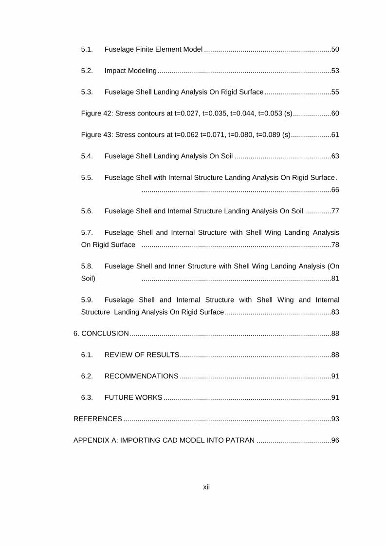
Figure 76: Laminate Modeler Screenshot -3 ......................................................... 100

Figure 77: Laminate Modeler Screenshot -4 ......................................................... 100

Figure 78: Laminate Modeler Screenshot - 5 ........................................................ 101

Figure 79: Laminate Modeler Screenshot – 6 ....................................................... 101

Figure 80: Laminate Modeler Screenshot – 7 ....................................................... 102

Figure 81: Solution steps, Screenshot -1 .............................................................. 103









xxi

Figure 90: Solution steps, Screenshot -10 ............................................................ 108










Figure 100: Solution steps, Screenshot -20 .......................................................... 115



Figure 103: Impact Velocity (m/s) vs. Maximum Deflection Graph (m) .................. 118

xxii

LIST OF NOMENCLATURES

A Extensional stiffness matrix

Aij Components of extensional stiffness matrix

aplate Edge length of plate

na Acceleration at step n

1na Acceleration at step n+1

1'na Estimated acceleration at step n+1

The distance that the impactor and the target approach

one another

max Maximum distance that the impactor and the target

approach one another

Time derivative of

Time derivative of

B Coupling stiffness matrix

c Speed of sound

C Damping matrix of the structure

P Deflection of plate

D Bending stiffness matrix

1'nd Estimated displacement at step n+1

nd Known value for displacement at step n

t Time step

i Strain component in i-directon

ext

nF 1 Vector of externally applied loads at step n+1

KP Spring constant of plate

K Stiffness matrix of the structure

k1’ Parameter given by Equation (6)

k2’ Parameter given by Equation (6)

L Minimum element length

xxiii

M Mass matrix of the structure

m Constant related to . (see Table 2)

1m Mass of impactor

2m Mass of target

Ni In plane force in i-direction

n’ Parameter given by Equation (11)

P Impact force

q0 Peak value of distributed force on an elliptical area

ijQ Components of stiffness matrix in principle axes

ijQ Components of stiffness matrix in laminate axes

r Constant related to . (see Table 2)

Density

R1M 1st principle radius of curvature of impactor

R1m 2nd principle radius of curvature of impactor

R2M 1st principle radius of curvature of target

R2m 2nd principle radius of curvature of target

S Safety factor

s Constant related to . (see Table 2)

i Stress component in i-direction

ij Shear stress component in ij-direction

u Position variable

nu Position at step n

1nu Position at step n+1

u Time derivative of u

nu Time derivative of nu

1nu Time derivative of 1nu

u Time derivative of u

nu Time derivative of nu

1nu Time derivative of 1nu

xxiv

1'nV Estimated velocity at step n+1

nV Known value for velocity at step n

1v Poisson’s Ratio of impactor

2v Poisson’s Ratio of target

V1 Velocity of impactor

V2 Velocity of target

V Initial relative velocity of impactor

maxw The highest eigenvalue in the system

Fraction of critical damping in the highest mode

1

CHAPTER 1

INTRODUCTION AND LITERATURE REVIEW

1.1. Introduction to Unmanned Aerial Vehicles

Unmanned Aerial Vehicle (UAV), as the name implies, are operated autonomously

or remotely, and they are used for reconnaissance purposes, as target/drone, or as

experimental platform for research/development. Nowadays their civil use and

military use is rapidly increasing. For instance it is claimed that in the future all the

fighter aircraft will be unmanned. The roots of UAVs are the very first Remote

Piloted Vehicles (RPV) in the beginning of 20th century [1]. During Second World

War UAVs are used to train AA Gunners. After 1950, design and production of

UAVs is accelerated and nowadays there are a number of classes of UAVs. Low

cost, multipurpose capability and keeping human away from the danger zones are

the most important reasons why UAV’s have become so popular. Current demand

on the UAV platforms and ongoing research activities into UAVs also show that in

the next 15 years there will be more unmanned platforms operating in the fields. [2]

1.2. Classification of Unmanned Aerial Vehicles

Mission profile is an important parameter that can be used to classify UAVs. The

duration they can operate without landing and the distance they can go is closely

related to their gross weight. Flight altitude is also a significant parameter and takes

place in classification. According to Unmanned Vehicle Systems International [3] the

classification of UAVs is given in Table 1. Figure 1 displays some examples of

unmanned air vehicle.

2

Table 1: Classification of UAVs [3]

UAV CATEGORIES Range

(km)

Flight

Altitude (m)

Endurance

(hour)

Maximum Take-Off

Weight (MTOW)

Tactical UAV

Micro <10 250 1 <5

Mini <10 150-300 <2 <30

Close Range Tactical 10-30 3000 2-4 150

Short Range Tactical 70-200 5000 3-6 200

Medium Range >500 14000 6-10 1250

Medium Range Endurance >500 8000 10-18 1250

Low Altitude Deep Penetration >250 50-9000 0.5-1 350

Low Altitude Long Endurance >500 3000 >24 <30

Medium Altitude Long Endurance >500 14000 24-48 1500

Strategic UAV

High Altitude Long Endurance >2000 20000 24-48 12000

Special Purpose UAV

Unmanned Combat Aerial Vehicle approx.

1500 10000 approx. 2 10000

Lethal 300 4000 3 to 4 250

Decoy 0 to 500 5.000 < 4 250

Stratospheric > 2000 >20000 &

<30000 > 48 TBD

Exo-stratospheric TBD > 30000 TBD TBD

Space TBD TBD TBD TBD

Figure 1: Examples for Different UAV Types: (a) Micro, (b) Mini, (c) Tactical, (d) Medium Altitude Long Endurance (MALE), (e) High Altitude Long Endurance (HALE)

3

1.3. METU “Güventürk” Mini Unmanned Aerial Vehicle

METU “Güventürk” Mini UAV System is designed and built in METU Aerospace

Engineering Department UAV Laboratories with the financial support of State

Planning Organization in 2005. With embedded original autopilot system,

“Güventürk” is capable of flying autonomously and accomplishing a reconnaissance

mission. Hand launching, extremely low noise signature and belly landing features

of “Güventürk” make it easy to operate in the field.

METU Mini UAV has duration of 1 hour and minimum 10 km of operational range.

Real time continuous telemetry data allows a clear view of the field from above. The

wingspan is 220 cm and MTOW is about 4.5 kg. Two photographs of “Güventürk”

during hand launch and belly landing are shown in Figure 2. More information about

“Güventürk” is given in Chapter 4.

Figure 2 Hand launch (top) and belly landing of “Güventürk”

4

1.4. Impact Phenomenon

Impact is a transient physical excitation and causes a force to be applied for a very

short period of time. When two bodies come into contact together with some velocity

a certain amount of impulse arises at the contact zone in both bodies. For the

impact of particles impulse is normal to the particles’ contact plane. However, for

more complex bodies there is a region of contact through which the impact loads are

induced on the impactor and the target material, and deformation on both bodies

occur due to the impact [4]. Impulse forces on this deformed surface are associated

so that there is no interpenetration of the bodies. In other words, forces prevent

overlapping of bodies.

A sample drawing of center impact and eccentric impact is given in Figure 3. In a

general impact case between two bodies B and B’, the term “incidence” refers to the

moment at which a point C on the body B is in contact with a point C’ on the body B’.

Incidence time is the initial instant of the impact. If at least one of the two bodies

have a smooth surface at C or C’, there is a tangential plane passing through C

and/or C’.

Referring to Figure 3, if rC is the vector from G to C and rC’ is the vector from G’ to

C’; the impact is called “Center Impact” if rC and rC’ are perpendicular to the

tangential plane. Otherwise, the impact phenomenon is called “Eccentric Impact”.

Figure 3: Scheme of Center Impact (left) Eccentric Impact (right)

5

The impulse caused by the impact of bodies results in a deformation at the contact

area. Impact induced deformation is dependent on the impact velocity, contact area,

contact duration and material hardness. Unquestionably, the relative velocity of the

bodies is the most important parameter when characterizing an impact case. Hyper

speed impacts; for instance, involves projection velocities of more than 10km/s [5].

Such high velocities can be achieved by gas guns or electromagnetic guns;

however, experiments are limited after 9km/s since it is impractical to measure

pressure waves with the current technology of devices. To give an example; hyper

velocities address strain rates to be as much as 106 s-1; whereas, car accidents

have a strain rate from 10-2 s-1 to 102 s-1 [6]. Figure 4 shows a simple diagram of the

relation between sample event and impact velocity.

Figure 4: Impact velocities of sample events [9]

6

Due to the low strain rates, low velocity impacts are easier to examine. If the relative

velocity of two bodies is less than 10 m/s then the impact phenomenon is

considered to be low velocity impact. Although high velocity impacts result in high

strain rates and high damage on the composite structure, the importance of low

level impact should not be underestimated. Low level impacts may result in internal

damage on the composite that may not be visible by naked eye [7]. Internal

damage caused by low velocity impact can be examined in two categories:

interlaminar damage which is called “delamination”; and intralaminar damage which

is transverse ply cracking [8].

Belly landing cases of mini UAVs are in low velocity impact class; therefore,

designers should spend enough time on analyzing landing loads and their possible

effects. According to the operational use of the UAV necessary improvements

should be made on the composite parts.

1.5. Composite Materials

Composite material refers to the material systems that are made from two or more

materials with different material properties. Fiber reinforced composite materials are

widely used in aerospace industry. In fiber reinforced composites fibers and the

matrix material form the two main constituents of the composite material. Fiber gives

the strength of the product whereas matrix builds up the integrity. The use of two

main constituents causes the composite material to behave anisotropically.

There are many fiber material types used in composite materials. Carbon, E-glass

and Kevlar are the most often used fabrics in aircraft structures. When these fabrics

are cured with a resin system such as epoxy, the resulting structure becomes stiff

and lightweight compared to metal counterparts. Different combinations (i.e. layups)

of these fabrics result in different composites parts and they have different

mechanical properties in terms of strength, stiffness, wear resistance, fatigue life,

thermal insulation, thermal conductivity, weight, acoustical insulation and

temperature dependent behavior [7]. Impact behavior of composites is under

investigation of researchers since the beginning of 1980’s [8]. After the year 2000,

the research is accelerated. A number of experiments are conducted in order to

understand the buckling, cracking, delamination, shear-out and fiber fracture

characteristics of composite laminates [9]. Effect of laminate thickness and

7

resin/fibre volume fraction on impact is also studied widely [10], [11]. Experiments

on glass-fiber-epoxy-matrix are almost completed [12].

The studies so far showed that by having a good design, use of composite materials

can be very advantageous. Laminated patterns can be built up so that necessary

stiffness in the required direction can be obtained. High stiffness-to-weight and high

strength-to-weight results can be achieved.

A final important feature about the composites is their high corrosion resistance and

excessive outdoor weathering ability.

.

1.6. Belly Landing UAV’s

For mini UAVs, belly landing is a good solution for weight and cost reduction and

simple operation. Firstly, the weight of the UAV can be decreased while maintaining

the integrity since the landing gears and gear struts are omitted. Moreover, there is

no need to stiffen the regions of fuselage where landing gear struts are attached.

Secondly, landing gear carries impact loads and needs to be designed and

manufactured accordingly. Omitting landing gear shortcuts the important design and

manufacturing process; to put differently, it is cost effective to employ belly landing

UAV’s. Even high speed UAVs are using this feature. For a turbine powered UAV

designed by University of Salt Lake City belly landing is decided since conventional

configuration has a drag and weight penalty [16]. Finally, belly landing enables the

UAV to take off and land from anywhere; in other words, a proper runway is not

needed. A simple hand launch allows the UAV to climb to operating altitude and

perform the mission. When the mission is completed, the UAV simply lands on the

grass or gravel.

Due to the advantages mentioned above there are numerous belly landing UAVs in

the market.

METU “Güventürk”, AeroVironment RQ-11 Raven, AeroVironment FQM-151

Pointer, Boeing ScanEagle UAV, BAI's Javelin and AAI’s Aerosonde are some

examples of belly landing UAV platforms.

A photo of “Güventürk” during belly landing is given in Figure 2.

8

1.7. Objective of the Study

The scope of this study is to help the designer in making design decisions for a mini

UAV that is tolerable to low velocity impact loads. To achieve this aim, “Güventürk”

mini UAV that is designed and built by Middle East Technical University Aerospace

Department is analyzed.

Low velocity impact phenomenon is examined in second chapter in detail. The

theory of an approach introduced by Greszczuk [17] is examined in details.

Greszczuk assumes that low velocity impact is “quasi-static” and proposes that the

impulsive force on a target caused by an impactor can be replaced with a static

force. The application area of the force can also be found. The impact problem can

then be solved analytically. At the end of the second chapter, it is shown that for

special class of orthotropic laminates, for which elastic properties are orientation

independent, the approach of Greszczuk can be followed.

In the third chapter, the details of implicit and explicit methods are given. They are

compared in terms of their applicability on finite element analysis problems.

MSC.Software Programs are also introduced in Chapter 3. Then, the method

introduced by Greszczuk is applied on fixed steel plates. The force on the steel plate

caused by an impactor is found and applied on the steel plate as static load.

Maximum deformations for different test cases are found. Then, test cases are

remodeled in MSC.Patran and explicit dynamic finite element solution method is

applied to find the deformations calculated previously. The results are compared

and applicability of Hertzian Contact Law is discussed. At the end of the third

chapter, the same comparison is made again for a composite plate.

Chapter 4 is dedicated to “Güventürk” Mini UAV. System description and

specifications and brief information about the production of its composite parts is

given. Belly landing condition of “Güventürk” is discussed in detail.

In Chapter 5, a complete analysis of “Güventürk” is given. Fuselage finite element

model is introduced. Following a buildup approach, sequential analyses including

fuselage shell, fuselage with internal structure and fuselage with wing are

completed. Extra effort is given to the analyses concerning the different stacking

sequences of fuselage composite laminates. Several test runs are executed for

fuselage with internal structure case. The effect of changing stacking sequence on

maximum stress is compared with simple plate analysis. Then, an alternative target

9

surface is examined. Soil is modeled as an elastic material and all analyses are

repeated as the landing surface changes from rigid to soil.

Chapter 6 is the conclusion part; therefore, all the results are summarized and

comments are given. A list of suggested future works is also developed.

10

CHAPTER 2

LOW VELOCITY IMPACT LOAD AND STRESS ANALYSIS

2.1. Low Velocity Impact

Impact phenomena can be categorized based on the impactor’s relative velocity with

respect to the target. Typically, an impact case with an approach velocity below

10m/s is considered as “Low Velocity Impact”. In this section low velocity impact

phenomena is introduced briefly and a simplified method of analysis of low velocity

impact behavior of isotropic and composite plate like structures is demonstrated. It

should be noted that the belly landing of a mini unmanned air vehicle on ground falls

under the low velocity impact phenomena because the vertical descent speeds of

such air vehicles are in general less than 10 m/s.

For low velocity impact cases with impact velocity below 10-2m/s static equilibrium

(∑F= 0) can be assumed. If the impact velocity is between 10-2m/s and 10m/s, then

the force equilibrium is assumed to be quasi-static. (∑F≈ 0)

Low velocity impact assumption can be made for a span of problems including

general engineering problems, aircraft belly landing events or even slow car

accidents.

2.2. Determining the Impact Load by Considering the Low Velocity Impact

as “Quasi-Static”

When an impactor approaches and impacts a target, the impact causes a time

dependent pressure field. As a result of the pressure, stress is observed in the

target which may eventually cause failure. To find out the amount of stress, the

pressure should be calculated first. For low velocity impact problems Greszczuk [17]

proposed an analytical approach to design for impact response. Such an analytical

treatment was proposed to address the issue of having a criterion for determining

how the various properties of the target and the impact parameters influence target

11

damage. Especially for composite targets the availability of different composite

material types and variety of design parameters, which can be adjusted to come up

with different laminates, necessitates the use of simple analytical approach to

design such composite structures subjected to impact loading. It should be noted

that analytical approach does not have to provide close to exact impact response for

all impact speeds. If the analytical approach allows one to make a qualitative

comparison of impact responses of the various design alternatives, then it can be

used in preliminary design stage to decide on the laminate configuration.

The approach in studying the response of isotropic and composite materials to low

velocity impact consists of three major steps [17]. These steps are:

Determination of impactor induced surface pressure and its distribution

Determination of internal stresses in the target caused by surface pressure

Determination of failure modes in the target caused by the internal stresses

In the simple analytical solution of the low velocity impact response of plate like

structures, the magnitude and distribution of pressure distribution in the target can

be obtained by combining the dynamic solution to the problem of impact of solids

with the static solution for the pressure between two bodies in contact. Thus, in this

method by applying the Hertz Contact Law [17] this dynamic problem can be

converted into a static problem. Hertz Law states that the magnitude and the

application area of the force caused by the impact can be estimated by an analytical

approach. In order for the Hertz Law to be applicable, following assumptions have to

be made:

The impactor is linear elastic

Contact duration of the target and impactor is relatively long compared to

their natural periods; in other words, vibrations can be neglected.

The impact is normal to the surface.

12

Figure 5: General Impact Case

In the simple approach, for a general impact event shown in Figure 5, it is assumed

that Hertz Law that was established for statical conditions applies also during

impact. Therefore, it is possible to calculate the magnitude and distribution of the

impact force. At the time of impact, the rates of changes in velocity of target and

impactor are given by [17]:

Pdt

dVm 1

1 , Pdt

dVm 2

2 (1)

where 1m and V1 are the mass and the velocity of the impactor, and 2m and V2 are

the mass and the velocity of the target.

Approach velocity is the derivative of the distance, , that the impactor and target

approach one another:

21 VV (2)

Assume that the principle radii of curvature of impactor at the point of contact are

R1m and R1M. And also assume that the principle radii of curvature of target at the

same point are R2m and R2M. According to Hertz Law, the contact area is an ellipse

with major and minor axes being [18]

R2m R2M

V2, m2

V1, m1

Planes of principle curvatures

13

3/1

21 ''2

3RCkkPma (3)

3/1

21 ''2

3RCkkPrb (4)

where CR is a term that takes into account the curvature effect and it is given by

[17]:

MmMmR RRRRC 2211

11111 (5)

For isotropic impactor and targets k1’, k2’ are given by:

1

2

11

1'

E

vk ,

2

2

22

1'

E

vk (6)

For the general case of impact between two nonisotropic bodies of revolution k1’ and

k2’ are yet to be defined. These are the parameters that take into account the elastic

properties of the impactor and the target.

In addition, m and r are constants and they are related to a parameter defined in

by Equation (8). m, r values are given in Table 2 after calculating from Equation

(8) and RC from Equation (7).

MmMmR RRRRC 2211

11111 (7)

2

1

2211

2

22

2

11

2cos1111

211

11

arccos

MmMmMm

Mm

R

RRRRRR

RRC (8)

In Equation (8) is the angle between normal planes containing the curvatures R1m

and R2m.

14

Table 2 Values of Parameters m, r, and s

0° 10° 20° 30° 40° 50° 60° 70° 80° 90°

m 6.612 3.778 2.731 2.136 1.754 1.486 1.284 1.128 1.00

r 0 0.319 0.408 0.493 0.567 0.641 0.717 0.802 0.893 1.00

s - 0.851 1.220 1.453 1.637 1.772 1.875 1.994 1.985 2.00

The total deformation of both impactor and the target is given by [17]:

3/12

21

22

256

''9

RC

kkPs (9)

If the above equation is solved for contact force one gets:

2/3'nP (10)

where,

3

21 ''3

16'

s

C

kkn R (11)

In Equation (9) and Equation (11) parameter s is given in Table (2).

If Equation (2) is differentiated with respect to time, combined with Equation (1) and

the result is substituted into Equation (10) following equation is found:

2/3'Mn (12)

where,

21

11

mmM (13)

If both sides of Equation (12) is multiplied by and integrated, following result is

obtained:

2

5

22 '5

4MnV (14)

V is the initial relative velocity of the impactor at time zero. At the time of maximum

deflection, max , the rate of deflection, , becomes zero; hence maximum

deflection can be determined as:

5/22

max'4

5

Mn

V (15)

Substituting Equation (11) into Equation (15) and combining it with Equation (10) the

impact force can be written as:

15

5/32

'4

5'

Mn

VnP (16)

Having found the impact force, the pressure distribution can now be determined. In

case of contact problem involving solids of revolution, the force distribution has been

shown to be of the form [17]:

2

2

2

2

0, 1b

y

a

xqq yx (17)

where q0, a and b can be found from the following relations:

ab

Pq

2

30 (18)

3/15/3

25/2

214

5'''

2

3

M

VnCkk

r

b

m

aR (19)

k1’ and k2’ is given in Equation (6) and can be used if the impactor and the target are

isotropic solids.

It should be noted once again that k1’ and k2’ given by Equation (6) can be used if

the impactor and the target are isotropic solids. In addition, if the impactor is

assumed to be rigid compared to the target k1’ can be neglected. For composite

targets if the designed laminate is quasi-isotropic then an equivalent modulus of

elasticity can be determined for the target material and k2’ given by Equation (6) can

still be used. It has been reported by [17] that no closed form solution exists for k2’

for generally orthotropic solids. It is also reported that an approximate numerical

solution for k2’ for generally orthotropic solids shows that k2’ is relatively insensitive

to the fiber orientation. The parameter k2’ for a generally orthotropic material can

also be determined experimentally. For instance for a spherical indenter

( mR1 = MR1 =R) and flat target mR2 = MR2 = , one can obtain a relation for k2’ in

terms of contact load P, and total deformation by performing a static indentation

test. Thus, from the knowledge of contact load P and the deformation of the target,

k2’ can be determined.

16

2.3. Quasi-static Low Velocity Impact Analysis of Composite Laminates

Low velocity impact damage on composite plates can be analyzed experimentally or

by means of finite element programs. There are numerous computer codes which

can solve this type of impact programs such as MARC, ANSYS or NASTRAN. In the

literature, there are a number of studies covering impact analysis of composites

considering different cases.

In this study, applicability of Hertz Method to analyze the behavior of composite

plates will be investigated. Details of the method are given in the previous section of

this chapter.

In this section simplified analytical method of analysis is performed by utilizing the

Hertz Contact Law to determine the loading due low velocity impact. The method is

applied to composite quasi-isotropic laminates so that Equation (6) can be used in

the calculation of constants k1’ and k2’. In chapter 3 results of the simplified method

are also compared with the results of explicit finite element solution of the low

velocity impact problem. This way one can form an opinion about the applicability of

the simplified analytical approach and decide if such the outcome of such an

approach can be used as a criterion for determining how the various properties of

the target and the impact parameters influence the impact response.

There is a special class of orthotropic laminates for which the elastic properties are

independent of orientation. In such laminates in-plane stiffnesses and compliances

and all engineering constants are identical in all direction [19]. The main property of

quasi-isotropic laminates is such that all shear coupling coefficients are zero. Thus,

the laminate can be assumed to be quasi-isotropic if A11=A22 and A16=A26=0. In

general any laminate of Sn

n

nn

1/.../

2//0 or

Snn/.../

2/ lay-up is quasi-

isotropic for any integer value greater than or equal to 2.

The in-plane stress mid-plane strain relations are defined by the classical lamination

theory.

12

2

1

66

2212

1211

12

2

1

00

0

0

kkQ

QQ

QQ

(20)

Transformation to laminate axes yields:

17

xy

y

x

kkxy

y

x

QQQ

QQQ

QQQ

662616

262212

161211

(21)

Figure 6: Cross section of an N-layered laminate

For the N-layered laminate given in Figure (6), the extensional stiffness is given by:

N

k

kkkijij zzQA1

1)( (22)

For quasi-isotropic laminates in-plane force resultant mid-plane strain relations are

then:

xy

y

x

ss

yyxy

xyxx

s

y

x

A

AA

AA

N

N

N

00

0

0

(23)

By making use of Eq. (23), in-plane moduli of the composite plate can be found by:

xx

xyyyxxyx

At

AAAEE

2

(24)

where, t is the thickness of the laminate. The effective Poisson’s Ratio can also be

determined as:

yy

xy

xx

xy

A

A

A

Av (25)

Thus, for quasi-isotropic laminates effective elastic Modulus and Poisson’s Ratio

can be used for the calculation of the constant k2’ in Equation (6) and the rest of the

18

steps described in the previous section can be followed in order to obtain the

magnitude and the application area of the impact force due to low velocity impact.

19

CHAPTER 3

LOW VELOCITY IMPACT ANALYSIS WITH FINITE ELEMENT METHOD

3.1. Implicit Method

The majority of finite element programs use implicit methods to carry out a transient

solution of structures subjected to time varying loads including impact loads.

Normally, these programs use Newmark schemes to integrate in time [20]. If the

current time step is step n, a good estimate of the acceleration at the end of step n +

1 will satisfy the following equation of motion:

ext

nnnn FKdCVMa 1111 '''

(26)

where

M = mass matrix of the structure

C = damping matrix of the structure

K = stiffness matrix of the structure

ext

nF 1 = vector of externally applied loads at step n+1

1'na = estimated acceleration at step n+1

1'nV =estimated velocity at step n+1

1'nd =estimated displacement at step n+1

Implicit methods are solved in time by applying Newmark method. [20]

Considering the equation of motion:

2

2

1tutuu (27)

20

Newmark states that, the first time derivative in the equation of motion can be solved

as:

utuu nn

1 (28)

where,

1)1( nn uuu 10 (29)

Thus, equation (28) can be rewritten as:

tutuuu nnnn 11 )1( (30)

Newmark also applied mean value theorem to the displacement equation:

2

12

1tutuuu nnn

(31)

where,

12)21( nn uuu 10 (32)

Therefore, equation (31) becomes:

2

1

2

12

21tututuuu nnnnn

(33)

Equation (33) and (30) can be rewritten as the estimates of displacement and

velocity:

2

1

2

1 '2/))21((' tatatVdd nnnnn (34)

tataVV nnnn 11 ')1(' (35)

(33) and (34) can be rewritten as:

2

11 '' tadd nnn (36)

taVV nnn 11 '' (37)

where, nd and nV are known or predictive values, and are constants, t is

time step.

Substituting (36) and (37) into (26)

ext

nnnnnn FtadKtaVCMa 1

2

111 '''

(38)

nn

ext

nn KdCVFatKtCM 11

2 ' (39)

residual

nn FaM 11* (40)

By inverting the matrix *M accelerations can be found.

21

Implicit solutions are unconditionally stable; therefore, time step size is chosen

according to the required accuracy.

3.2. Explicit Method

Matrix solutions are not required for explicit methods. The equation of motion is

used to obtain acceleration.

ext

nnnn FKdCVMa (41)

nn

ext

nn KdCVFMa (42)

If internal forces are defined as:

nnn KdCVF int (43)

Equation (41) becomes:

int

n

ext

nn FFMa (44)

int1

n

ext

nn FFMa (45)

M matrix is diagonal and inversion of M is trivial. Therefore, Equation (45) is set of

independent equations. Assuming acceleration is constant through the time step,

velocities and displacements are found by central difference method.

21

21

21

21

2 nn

n

nntt

aVV (46)

21

211 nnnn tVdd (47)

The loop given in Figure 7 is carried out for each time step.

Figure 7: Explicit Method Scheme [20]

Grid Point Accelerations

Grid Point

Velocities

Element Strain

Rates

Element Stresses

Element Forces at Grid Points

Grid Point

Displacements

Element Formulation and Divergence

Operator

Constitutive Model and Integration

Element Formulation and Gradient

Operator

Central Difference Integration in Time

22

Explicit methods can be made unconditionally stable if the time step is chosen to be

less than the time taken for a stress wave to cross the smallest element in the mesh.

Typically, explicit time steps are 100 to 1000 times smaller than those used with

implicit codes.

Figure 8: Time Step and Stress Waves Relationship

Figure 8 shows the propagation of stress waves in a media.

where,

L = Minimum element length

c = Speed of sound

Δt = time step

The stability limit of explicit method is the duration that the stress wave crosses the

smallest element. It can be found by the following relation:

2

max

12

wtcritical (48)

where,

maxw = The highest eigenvalue in the system

= Fraction of critical damping in the highest mode

23

3.3. Comparison of Implicit and Explicit Methods

Differences between implicit and explicit methods are tabulated in Table (3).

Table 3: Comparison of Implicit and Explicit Methods

Implicit Methods Explicit Methods

Bigger time step Small time step

Big matrices and matrix inversion

required

No big matrices and matrix inversion

by having a diagonal matrix

Solution procedure complicated with

increasing degree of nonlinearities

Robust solution procedure even for

high degree of nonlinearities

The computational time is relatively long for explicit methods due to the small time

step. On the contrary, matrix operations are simpler and reduce the calculation

steps. If the problem includes nonlinearities such as large displacements, plasticity

of material, large strain values or pressure spikes, the explicit method is still reliable.

Computational cost of a problem linearly increases with the problem size for the

explicit method; whereas, it increases exponentially for the implicit method. Duration

of the problem is important as well. As the duration increases, implicit method

becomes more applicable. Cost of implicit and explicit methods for various cases is

given in Figure 9.

Figure 9: Cost of Methods for Various Cases [8]

For impact problems with an impact velocity greater than 1 m/s, it is essential that

explicit method is applied.

The impact velocity of a belly landing UAV is most generally between 10-1 m/s and

100 m/s. This velocity regime can be called as “low velocity impact”. For low velocity

impacts, strain rate is small; therefore, quasi-static approach can be followed.

24

3.4. MSC.Patran/Nastran

MSC.Patran is a software system, used primarily in mechanical engineering analysis

[21]. It is comprised of engineering modeling functionalities, geometry access from

external programs, analysis modules like thermal and fatigue, result visualization

and reporting.

MSC.Nastran is a general purpose finite element analysis solution for small to

complex assemblies [22]. Nastran provides a wide range of modeling and analysis

capabilities, including linear statics, displacement, strain, stress, vibration and heat

transfer.

In this study skin model of “Güventürk” Mini UAV has been completed in Dassault

System’s CATIA v5.r13 [23] and imported into MSC.Patran. Patran is used for

meshing outer skin and modeling the internal structure. Later, the whole model is

laminated by Laminate Modeler Tool of MSC.

The process of importing a model into MSC.Patran is given in Appendix A.

The details of the Laminate Modeler Tool are explained in Appendix B.

3.5. MSC.Dytran

Dytran is an explicit finite element analysis (FEA) software for analyzing complex

nonlinear behavior involving permanent deformation of material properties or the

interaction of fluids and structures [24].

Generally, problem in space is solved by FEM and problem in time is solved by

explicit time integration with small time increments. MSC.Dytran applies Lagrange

Finite Element Technology and/or Euler Finite Volume Technology. Problem in time

is solved by central difference integration.

Grid points are fixed to the body locations when Lagrange solver is applied. As the

body moves or deforms grid points relocates with the body; in other words, in

Lagrangian meshes elements are of constant mass. In another word, in Lagrangian

meshes since the material points remain coincident with mesh points, elements

deform with the material. Therefore, elements in a Lagrangian mesh can be severely

distorted. A typical Lagrangian mesh is illustrated in Figure 10 which shows the

undeformed and deformed configurations.

25

Figure 10: Lagrange Finite Element Technology – Elements of Constant Mass

On the other hand in Eulerian meshes, grid points are fixed to space.. Eulerian

mesh acts as a fixed frame of reference; moreover, energy, mass and momentum

transfers through elements. Figure 11 shows a typical Eulerian mesh at two different

times. It is seen that the mesh does not change as the material passes through it.

Figure 11: Euler Finite Volume Technology – Elements of Constant Volume

As it is mentioned in Section 3.2, in order to have a stable solution the time step size

must be less than the duration of a stress wave to travel through the smallest

element. For a problem with many elements, it is a long process to accomplish the

eigenvalue analysis shown in Equation (48). An approximate method called Courant

Criterion is applied in MSC.Dytran solver. Courant Criterion states that, [9]

c

Ltcritical (49)

where,

L is the smallest element dimension, and the speed of sound can be approximated

as:

Ec for 1-D elements (50)

21 v

Ec for 2-D elements (51)

where,

E = Young’s Modulus

v = Poisson’s Ratio

= Density

26

Critical time step size is calculated for the whole model; that is for all of the

elements, by using Courant Criteria. After calculating the critical time step values for

all elements, the smallest one is multiplied by a safety factor, S.

criticaltSt (52)

The default safety factor is 0.666 for MSC.Dytran. However it can be reset to 0.9 for

the models with Lagrangian elements only [9].

3.6. Examples of Low/High Velocity Impact Problem Solutions

In this section low velocity impact demonstrations are performed. The solutions are

performed by modeling the impact phenomenon as a quasi-static event as

described before and by performing explicit finite element solution using MSC

Dytran. The impactor is assumed to be rigid to concentrate on what is happening in

the target material. As for the target material for the initial solutions an isotropic

material steel is used. Later on a quasi-isotropic laminate is modeled and low

velocity impact solutions are performed.

In the initial analyses a rigid ball impactor of 0.1 m radius (rball) is projected to a steel

square plate target of 1 m edge length (aplate), as shown in Figure 12.

Figure 12: Impactor and Target

V aplate

aplate

rball

27

Properties of ball which is the impactor:

mrball 1.0

ballE (Rigid ball assumption)

impactV Varying

ballm Varying

Properties of steel plate which is the target:

aplate = 1m

PaE

mt

mkg

v

steel

11

3

102

005.0

/7850

3.0

Two different methods are used to solve this problem. In the first method, the impact

case is assumed to be quasi-static. Hertz Law, as explained in detail in the chapter

2, is applied and the impact force is calculated. Then, the impact force is then

applied as a static load to the plate and the problem is solved by MSC.Nastran

utilizing linear static solver. In this method since the low velocity impact is modeled

as a quasi-static event, it is expected that a static finite element solution might

provide reasonable results especially for low impact velocities.

Secondly, the same impact problem is modeled in MSC.Patran and the explicit finite

element analysis is performed by MSC.Dytran.

Finally, for different impact velocities of the ball, the solutions are compared and

applicability of Hertz Law is investigated.

3.6.1. Solutions with MSC.Nastran by assuming low velocity impacts; “quasi-

static” case

For a flexible, plate-like target, the surface pressure, area of contact and impact

duration will be functions of the parameters entering in Equation (15), and Equation

(18-19) as well as the bending stiffness of the plate and boundary conditions. For a

given impact velocity the impact load P will decrease as the flexibility of the target

increases [17]. Increase in target flexibility will also increase contact duration and

decrease the contact area. An approximate solution for the impact response of a

flexible target can be obtained by considering the deformations shown in Figure 12.

28

The case shown in Figure 13 indicates the local and overall deformation of flexible

target at the moment of maximum deflection.

Figure 13: Local and Overall Deformation of the Target

In Figure 13 P represent the maximum deflection of the plate and indicates the

Hertzian contact deformation.

According to Hertz Law, resulting impact force due to low velocity impact was given

in Chapter 2 as:

23

'nP (10)

where,

the distance that impactor and target get closer to each other due to

compression

For rigid impactor ball and plate case ballMm rRR 11 and Mm RR 22 .

Therefore, Equation (7) becomes:

ballR rC

21 (53)

On the other hand, Equation (8) yields

2/)0arccos(

For the value of 2/ Table 2 gives

α

P

t = 0

t > 0

0v

0v

29

m = 1

r = 1

s = 2

Therefore, Equation (11) becomes:

21

1

3

4'

kk

Rnn (54)

where;

01

1

2

1

1E

vk (Rigid ball assumption)

2

2

2

2

1

E

vk

If energy balance equation is written for the impact event shown in Figure 12 one

gets:

00

2max

2

1dPdPVm contactplateplateballball (55)

where,

Pplate

contact

KP

PP

and PK is the spring constant for the plate.

Substituting Equation (10) and pPplate KP into Eq.(55) and noting that

platecontact PP Equation (55) can be rewritten as:

3/2

3/522

5

2

2

1

2

1

n

P

K

PVm

P

ballball (56)

In the ball impact problem over a plate Equation (3) and (4) becomes identical which

means that impact area becomes circular:

3/1

214

3ballrkkPba (57)

In Equation (56) if the spring constant of the plate PK is known then the impact load

P can be solved iteratively. The plate spring constant PK can be determined easily

by performing a linear static analysis by MSC.Nastran. In the current example the

plate model is analyzed under 100 N concentrated load at the center of the plate,

30

and the maximum deflection is found as m41053.2 . Figure 14 shows the

displacement plot of this solution.

Figure 14: Calculation of Maximum Deflection of the Plate under 100N Load

Therefore; bending stiffness constant PK for this particular plate is:

mNE

PK P /

0453.2

100 (58)

After all the unknown variables, except the impact load P, in Equation (56) have

been calculated, P can be found by iteration. Force application area can also be

calculated from Equation (57).

Tables 4-6 give the impact loads which are determined from the solution of Equation

(56) for three different impactor masses and for five different impact velocities.

Table 4: Iteration of P for m=0.2kg

mball (kg) 0.2

Vball (m/s) 0.1 0.5 1 5 10

P (N) 28.045 140.372 280.83 1404.836 2810.071

Area (m2) 2,12E-4 3,63E-4 4,58E-4 7,82E-4 9,86E-4

Table 5: Iteration of P for m=2kg

mball (kg) 2

Vball (m/s) 0.1 0.5 1 5 10

P (N) 88.757 444.105 888,395 4443.456 8887.772

Area (m2) 3,12E-4 5,33E-4 6,72E-4 1,149E-4 1,448E-4

31

Table 6: Iteration of P for m=20kg

mball (kg) 20

Vball (m/s) 0.1 0.5 1 5 10

P (N) 280,83 1404,835 2810,071 14053,543 28108,941

Area (m2) 4,58E-4 7,83E-4 9,86E-4 16,86E-4 21,25E-4

The impact loads given in Table (4) and (6) are applied as concentrated forces in

the geometric center of the steel plate, and each case is analyzed in MSC.Nastran

and corresponding deflections are found. It should be noted that the right hand side

of Equation (56) is proportional to almost square of the impact load. Therefore, if the

impactor mass is increased by a factor then the impact load should increase by

square root of that factor. The results given in Tables (4-6) confirm this behavior. For

instance when the impactor mass is increased 100 times, from 0.2 kg to 20 kg, the

impact load increases by approximately 10 times. In a similar fashion in Equation

(56) impact velocity and impact load are approximately directly proportional to each

other. This relation is also reflected in Tables (4-6). When the impact velocity is

increased by a factor, the impact load also increases by the same factor. One last

comment about the results given in Tables (4-6) is that the 20 kg impactor mass

case combined with the impact velocities might put the problem out of the limits of

linear analysis.

The impact loads given in Table (5) are first applied as concentrated forces and later

on they are uniformly distributed on the steel plate over the circular impact area

determined by Equation (57). This analysis is accomplished for three different

velocity cases (0.1 m/s, 1 m/s, 10 m/s). Sample screenshots of MSC.Patran, for

these analyses, are given in Figures 15 and 16. Figure 15 gives the displacement

plot for the concentrated load case and Figure 16 gives the displacement plot for the

distributed load case.

32

Figure 15: Maximum Deflection for Concentrated Load, P=88.8N, m=2kg, V=0.1m/s

Figure 16: Maximum Deflection for Distributed Load, P=88.8N, m=2kg, V=0.1m/s

Meshing details of the distributed load case is given in Figure 17-18.

33

Figure 17: Meshing of Distributed Load Case

Figure 18: Meshing of Distributed Load Case (detail)

As it is explained in Chapter 2.3 the same low velocity impact problem is solved by

using a classical orthotropic laminate as the target material instead of a steel plate.

A composite laminate having four layer with a stacking sequence of [0o,90o,90o,0o] is

taken and as the layer material carbon/epoxy is chosen. After modeling the

carbon/epoxy laminate in MSC.Patran, the stiffness coefficient matrices A, B, D

matrices are determined as:

PaA

006+1.056000E000+1.14748E-003-4.756234E

000+1.14748E-007+2.937823E005+9.059633E

003-4.756234E005+9.059633E007+2.937823E

(59)

PaB

000+0.000000E000+0.000000E000+0.000000E

000+0.000000E005-1.52587E-006-3.81469E-

000+0.000000E006-3.81469E-000+0.000000E

(60)

34

PaD

002-2.027520E000+0.000000E000+0.000000E

000+0.000000E001-1.876079E002-1.739449E

000+0.000000E002-1.739449E001-9.405161E

(61)

As it was requested in Chapter 2.3, the in-plane extensional stiffness coefficients are

equal to each other and the in-plane coupling stiffness coefficients are negligibly

small. As a matter of fact from a theoretical point of view, the coupling coefficients

should turn out to be exactly zero for the particular laminate.

A11 = A22

A16 ≈ A26 ≈ 0

Therefore; the laminate can be regarded as quasi-isotropic and after determining the

effective modulus and Poisson’s ratio for the quasi-isotropic laminate, Hertz Law can

be applied.

From Equation (24) and (25), the effective modulus and Poisson’s ratio of the

laminate are determined as

E1 = E2 = 6.12E+10 Pa

v = 3.08E-02

Thickness of Carbon/Epoxy laminate used in the analysis is given by Turgut [25]:

t = 0.00053 m

KP is found again by modeling the plate in MSC.Patran and applying a concentrated

force, similar to the isotropic target case.

mNm

NKP /94.71

139.0

10

Following the same procedure a set of results is obtained for the impact load for

different impactor mass and impact velocities. For instance Figure 19 shows the

displacement plot of the composite plate for an impact load of 0.38 N which is

calculated for an impactor mass of 0.2 kg and impact velocity of 0.1 m/s.

35

Figure 19: Maximum Deflection for Concentrated Load, P=0.38N, m=0.2kg,

V=0.1m/s

3.6.2. Explicit finite element solutions of low velocity impact problems with

MSC.Dytran

Low velocity impact problems, which were analyzed by a quasi-static approach in

the previous sections, are solved by MSC.Dytran utilizing explicit finite element

solution. In order to solve the same problems by MSC.Dytran, the model is built

again in MSC.Patran. Boundary conditions of the plate, initial velocity of the ball and

material properties of both of them are given as input. In the analyses performed by

MSC.Dytran, there is no need to enter the contact area or duration of the impact

because MSC.Dytran calculates the necessary parameters automatically.

After the completion of modeling, each case solved in Part 3.6.1 is resolved with

MSC.Dytran.

A sample screenshot from MSC.Dytran analysis is given in Figure 20.

36

Figure 20: Sample screenshot from MSC.Dytran analysis

3.6.3. Comparison of quasi-static and explicit finite element solutions

The maximum plate deflections determined by the quasi-static analyses and explicit

finite element solutions are compared in Table 7 for the steel plate.

Table 7: Maximum Deflection of Steel Plate for mball = 2kg

mball (kg) 2

Vball (m/s) 0.1 1 10

Dytran Solution (m) -0.00011 -0.00109 -0.00777

Nastran Solution (m) -0.00023 -0.00225 -0.0225

Nastran Solution (m)

(force is uniformly distributed over the area given in Table 5 )

-0.00021 -0.00216 -0.0216

Table 7 shows that application of the impact load in a concentrated fashion or as a

uniformly distributed load over the area of contact gives very close deflection results,

as expected. Tables 8 and 9 compare the maximum plate deflection for five different

impact speeds for impactor masses of 0.2 kg and 20 kg, respectively. It is observed

that explicit finite element solution consistently produces lower deflections compared

to the quasi-static solutions obtained by MSC.Nastran.

37

Table 8: Maximum Deflection of Steel Plate for mball = 0.2kg

mball (kg) 0.2

Vball (m/s) 0.1 0.5 1 5 10

Dytran

Solution (m) -0.00002 -0.00009 -0.00019 -0.00094 -0.00186

Nastran

Solution (m) -0.00007 -0.00036 -0.00071 -0.00356 -0.00711

Table 9: Maximum Deflection of Steel Plate for mball = 20kg

mball (kg) 20

Vball (m/s) 0.1 0.5 1 5 10

Dytran

Solution (m) -0.00051 -0.00248 -0.00467 -0.01483 -0.02442

Nastran

Solution (m) -0.00071 -0.00356 -0.00711 -0.0356 -0.0711

Figures (21-23) below are sketched by using the data given in Tables 7-9 As it can

be seen, the discrepancy between the result of quasi-static solution based on the

Hertz method and the explicit finite element solution increases as the impact velocity

increases. A graph drawn with more data points is given in Appendix E.

Figure 21: Comparison of Different Solution Methods for mball = 2kg

38

Figure 22: Comparison of Different Solution Methods for mball = 0.2kg

Figure 23: Comparison of Different Solution Methods for mball = 20kg

From the displacement results one conclusion that may be drawn is that the quasi-

static approach overestimates the resulting deformation of the target material. The

main reason for this could be due to the fact that in the quasi-static approach the

peak impact load is assumed to act at full magnitude. However, in real case there is

duration and the impact load increases from a zero value to peak value in a finite

time. The total impact duration could also be calculated from Equation (14).

Greszczuk [17] has calculated the total impact duration in his work from Equation

(14), and it is seen that the total impact duration is inversely proportional with the

impactor mass, as expected. Therefore, the impact duration is shorter if the mass of

the impactor is higher. In addition, in the work of Greszczuk [17] the variation of the

39

impact load with time is seen to a half sine wave which is in accordance with the

variation of impact deformation with time. It can be observed from Tables 7-9 that

when the mass of the impactor is increased the percent difference between the

quasi-static solution and explicit finite element solution decreases. This behavior is

attributed to the fact that when the mass of the impactor is increased the impact

duration decreases and the peak impact load is reached in a shorter time. Thus, the

deformation induced by the peak impact load approaches to the quasi-static case in

which the peak impact load is acting continuously. The discrepancy between the

quasi-static solution and explicit finite element solution might also be due to the

overestimation of the impact load in the quasi-static approach.

It should be noted that one could determine the variation of the impact load with time

as described by Greszczuk [17] and carry out a transient finite element analysis by

imposing a time varying force on the target material. It is expected that the result of

such an analysis could provide more close results to the results determined by

MSC.Dytran. However, in this study this work is not performed because the main

aim was to investigate the applicability of quasi-static approach in low velocity

impact problems. Such a transient finite element analysis based on a time varying

load is more time consuming compared to an MSC.Dytran analysis.

Based on the analysis performed on steel plate it can be concluded that quasi-static

approach may provide reasonable results for very low velocity impact problems.

However, the in the 10 m/s range the discrepancy between the results of the quasi-

static approach and MSC.Dytran solution can be very large especially at impact

speeds close to 10 m/s. Therefore, the quasi-static approach should not be relied

on.

For some of the cases MSC.Dytran is requested to output time history graphs.

Middle node is observed and z position vs. time graph is sketched. Figures 24 and

25 give the variation of the displacement of the center node of the plate with respect

to time for the 2 kg impactor corresponding to impact velocities of 0.1 m/s and 10

m/s, respectively. Displacement plots show that the plate bounces back following

the impact. The maximum displacement values given in Tables 7-9 are read from

these time history plots at the center node of the plate.

40

Figure 24: Z-Position vs. Time Graph for Steel Plate (m=2kg, V=0.1m/s)

Figure 25: Z-Position vs. Time Graph for Steel Plate (m=2kg, V=10m/s)

It should be noted that the vertical position (Z-Position) is given in mm. Initial

position of the steel plate is -0.15mm. Node 1729 is at the geometric center of the

steel plate.

(mm)

(s)

(s)

(mm)

41

For the composite plate case the analysis results are similar to the previous one.

Table 10 gives the results for the quasi-isotropic composite plate for an impactor

mass of 0.2 kg. It can be seen that for the composite plate there is a significant

difference between the peak deformation determined by the quasi-static approach

and MSC Dytran solution.

Table 10: Maximum Deflection of Composite Plate for mball = 0.2kg Vball (m/s) 0.1 0.5 1 5 10

Dytran

Solution (m) -0.00186 -0.00467 -0.00696 -0.01595 -0.02288

Nastran

Solution (m) -0.00528 -0.0265 -0.0529 -0.264 -0.529

Figure 26: Comparison of Different Solution Methods for mball = 0.2kg

3.7. Impact Analysis of Composite Plates With Different Materials and

Stacking Sequences

In this section the response of composite plates subject to impulsive loads is

investigated. The main aim is to provide insight to the effect of stacking sequence on

the stress and deformation response of the composite plate. As an initial analysis a

simple composite plate of 30cm edge length is modeled. Carbon-Epoxy Woven is

42

used as composite material. According to the test results by Turgut [25] Carbon-

Epoxy Woven has following material properties:

Table 11: Material Properties of Carbon-Epoxy Woven

E11 = 46.26 GPa G12 = 3.8 GPa

E22 = 46.26 GPa G23 = 2.7 GPa

ν12 = 0.03 G13 = 2.7 GPa

ρ = 1.19 × 10−6kg/mm3 t = 0.133 mm

Figure 27 shows the finite element model of the composite plate used in the

analyses.

Figure 27: Carbon-Epoxy Plate Model

As shown in Figure 27 plate is clamped from all sides and an impulsive force of

100kPa is applied for 0.5 s and solution is performed in MSC Dytran. The analysis is

repeated for different stacking sequences for 8 plies. Maximum stress and deflection

results are tabulated in Table 12.

43

Table 12: Maximum Stress and Deflection Results of Test Case

Stacking Sequence Max. Stress (MPa) Max. Deflection (mm)

[0/0/0/0]2 83.468 0.29666

[0/45/0/45]2 72.333 0.42215

[45/0/0/45]S 55.701 0.56534

[0/45/0/45]S 90.188 0.35234

[45/45/0/0]S 57.753 0.7908

[0/0/45/45]2 71.577 0.44096

[45/45/45/45]2 60.731 1.0889

[45/0/45/0]2 90.013 0.45616

[0/45/45/0]2 90.702 0.39593

[45/0/45/0]S 56.185 0.67569

[0/0/45/45]S 89.688 0.32402

[45/45/0/0]2 88.833 0.50402

From results given in Table 12 it is clear the stacking sequence significantly affects

the peak stress and deflection values of the composite plate. Such a simple study

shows that in designing composite structures one should make a stacking sequence

study to decide on the best lay-up configuration to use in the particular design at

hand.

The analysis above can be repeated if the impulsive force is replaced with an

impactor ball which is projected on a similar plate as shown in Figure 28.

Figure 28: Low velocity impact model of a ball impactor on a target plate

44

If a ball impactor with 10 mm radius is projected at a speed of 2 mm/s on a target

plate with 10 cm edge length the stress and maximum deflection varies as the

stacking sequence changes. Results for 6 different cases are tabulated in Table 13.

Table 13: Maximum Stress and Deflection Results of Test Case - 2

Stacking Sequence Max. Stress (MPa) Max. Deflection (mm)

[0/0/0/0]2 13.988 0.248

[45/45/45/45]2 14.061 0.251

[45/0/45/0]2 13.749 0.25

[0/0/45/45]2 13.894 0.251

[0/0/45/45]S 13.985 0.249

[45/0/0/45]S 14.217 0.249

The results for both impulsive force and low velocity impact show that stacking

sequence directly affects the stress and strain behavior of the whole laminate. This

phenomenon for “Güventürk” Mini UAV is analyzed in the following chapters.

45

CHAPTER 4

DESIGN AND STRUCTURAL LAYOUT OF “GÜVENTÜRK” MINI UAV

4.1. Description and Specifications

As the demand on Unmanned Aerial Vehicles increased, Middle East Technical

University Aerospace Department took part in a project financed by State Planning

Organization. Following the requirements of the project, METU Aerospace

Engineering UAV Research Group designed and built a Mini UAV that is capable of

performing observation, reconnaissance and surveillance missions autonomously

inside a mission range of 10 km.

“Güventürk” Mini UAV is a hand launched airplane with belly landing capability by

the virtue of folding propeller. The airplane is designed to carry an analog or IR

Camera. It was designed to be a lightweight platform so that it could be hand

launched. Maximum take-off weight of the airplane was limited to 4.5 kg with a

maximum payload weight of 0.5 kg. Long wing span of 2.20 m gives the opportunity

to have a small stall speed. 9 m/s stall speed makes belly landing easier. The

airplane is also equipped with the commercial autopilot MicroPilot [26] which can fly

the airplane autonomously.

A photo showing “Güventürk” after hand launch is given in Figure 29.

Figure 29 “Güventürk” in operation

The specifications of “Güventürk” are summarized in Table 14.

46

Table 14: Specifications of “Güventürk” Mini UAV

MTOW 4.5 kg Empty Weight 3 kg

Wing Span 2.20 m Length 1.35 m

Endurance 90 min Range 10 km

Maximum Speed 23.5 m/s (45kt) Stall Speed 9 m/s (17kt)

Cruise Speed 13.5 m/s Cruise Altitude 300 m

The solid model of “Güventürk” that was built in CATIA is the one of the basic

milestones of the whole design period. It is not only a visual representation of the

UAV, but also starting point of the CFD and structural analyses. In this study, the

skin of the aircraft is transferred from CATIA to MSC.Patran and belly landing

analysis is accomplished. CATIA model of the UAV is given in Figure 30.

Figure 30: Solid Model of “Güventürk”

47

CATIA model is used to form molds as well. After modeling the whole vehicle in

CATIA, a foam male mold is produced by the hot wire foam cutting CNC machine.

Female molds are made of polyester. During the production, carbon fabric is widely

used on this platform with epoxy matrix. Underneath of the fuselage is reinforced by

means of Kevlar which gives additional elasticity against the impact loading. Internal

structure is stiffened by balsa wood covered by carbon fabric.

The spar inside the wing is made of Styrofoam covered again by carbon fabric. The

spar is cut from a block of Styrofoam in the requested shape and thickness; then, by

vacuum bagging method it is covered by carbon fabric. Curing is completed at room

temperature. Schematic of spar and internal structure is given in Figure 31.

Figure 31: Schematic of spar and internal structure [25]

After the production of “Güventürk” mini UAV is completed it is divided into 5 parts:

Fuselage, horizontal tail, mid wing and two outer wings. In this way, maintainability

is improved and transportation is made easier.

A carry bag is also built to ease the flight test operations. The packed aircraft can be

made ready to fly in approximately 5 minutes. First, the middle wing and horizontal

tail is fixed to the fuselage by plastic screws; then, outer wings are attached to the

middle wing by sliding in through the spar holes; and finally, putting the battery on

board by a strip of Velcro.

4.2. Belly Landing

At the end of a successful mission, when “Güventürk” descends to the ground, the

only thing that is expected is a safe landing. During the final leg of approach electric

motor is cut off and the propeller folds. Then, the aircraft flies at minimum airspeed

48

possible which is very close to stall speed. As a result of the high aspect ratio of

wing, approach velocity is very low.

The aircraft approaches to the ground at 5°-10°; whereas, the approach angle

becomes smaller when altitude above ground level becomes 3-6 ft or 1-2 m.

Considering an ideal landing case, at the time of touch down, the approach angle

should be less than 3°.

The weight issue also becomes extremely important in belly landing for such mini

unmanned airplanes. Low weight implies low stall speed and for an airplane landing

on its belly if the stall speed is low, then the speed of the airplane can be reduced

further before touchdown. Therefore, low weight design of such mini unmanned

airplanes is a necessity also from landing point of view. Ideal landing would be a

landing without a glide which implies that the forward velocity of the airplane should

be almost zero. Such an ideal landing cannot be achieved in practice, however by

clever design the stall speed of the airplane can be reduced as much as possible. In

the current design high lift devices such as flaps were not integrated to the airplane.

Therefore, the landing speed of the airplane could not be decreased further. In

addition, depending on the mission requirements there were demands for installing

additional systems on the airplane which further increased the weight of the airplane

resulting in an increase in the stall speed. Under such circumstances the forward

velocity of the airplane during landing cannot be decreased. High forward speed is

not as critical as high vertical speed during landing. However, under certain

circumstances during the skidding period on the ground, an obstacle on the way

may induce high load on the airplane if the forward speed is high during landing.

Therefore, low forward speed is a desired requirement. In addition to low forward

speed, the vertical descent speed of the airplane is also a crucial factor in the

structural integrity of the airplane. During landing there can be unpredictable factors

that may prevent the air vehicle from a safe landing. Gust, for instance, might cause

the aircraft to suddenly hit the ground suddenly when the aircraft is in close

proximity to the ground. Based on the experience obtained during the flight tests of

“Güventürk” it is concluded that during windy weathers belly landing-associated

failures of the sub-structures of the airplane increased. Actually, when the wind

speed is high this can be used to advantage during landing by landing against the

wind so that the forward speed of the airplane can be decreased to such a level that

landing can be performed smoothly. However, in the windy weathers very frequently

49

there are changes in the wind speed and its direction which causes the pilot to lose

control and execute hard landing in order to prevent a full crash. Therefore, gust is

considered to be the major factor affecting the smooth or hard landing phenomenon

of the unmanned air plane. Another reason for a hard landing may be the external

pilot. Especially, an inexperienced pilot might land the airplane with a higher vertical

speed which may induce higher landing loads on the airframe. The advantage of

autonomous landing capability can be appreciated more during belly landing. With

autonomous landing the pilot related events causing hard landing may be

minimized. However, the main drawback in autonomous landing is the time

consuming experimentation that has to be carried out before successful landing can

be achieved.

In any case, it should be expected that during belly landing the airframe might be

exposed to impact loads due to various reasons which may not be always

controlled. Figure 32 shows “Güventürk” during a belly landing. This picture shows

an ideal landing on a grass-soil mixed ground.

Based on the explanations made in this section, it can be concluded that the impact

velocities encountered under most belly landing cases can be considered as low

velocity. Therefore, the main goal of this thesis, as it was mentioned in the

introduction section, is to perform the structural analysis of the airframe of the mini

unmanned air vehicle under low velocity impact loads that may be induced during

belly landing. The next section summarizes the low velocity impact analysis results

of the mini unmanned air vehicle and draws conclusions.

Figure 32: Belly Landing of “Güventürk”

50

CHAPTER 5

LOW VELOCITY BELLY LANDING ANALYSIS OF “GÜVENTÜRK”

5.1. Fuselage Finite Element Model

In this chapter, the belly landing analysis of “Güventürk” Mini UAV is accomplished

in light of the information obtained by the analysis made in third chapter. As it is

stated in Chapter 3.7, variation of stacking sequence significantly affects the peak

stress. In order to optimize the design of composite parts of “Güventürk”, the whole

fuselage model is analyzed by applying different layup configurations. The main aim

of this chapter is to accomplish a stacking sequence study for the fuselage and

guide the designer of “Güventürk” in fuselage manufacturing part. As a preliminary

study, analysis is executed for the fuselage skin only. Then, the fuselage is

combined with the internal structure, and that configuration is analyzed in detail.

Finally, the combination of wing and fuselage is analyzed to have some ideas about

the effects of belly landing on the whole structure. Because of the limitations in

computer resource and very long solution times of the explicit finite element solution

the vertical and horizontal tail plane is left out of the analysis. It should be noted that

based on the flight test experience of the air vehicle horizontal and vertical tail

structure is not affected adversely by the hard belly landing. Therefore, leaving the

tail system out of the analysis can be justified. However, as a future work the tail

system could also be included in the analysis to see the effect of belly landing on the

behavior of the tail system.

During the design of “Güventürk” Mini UAV, Dassault’s Computer Aided Three-

Dimensional Interactive Application “CATIA” v5 r13 was employed. Fuselage, wing,

tail and internal structure were modeled in detail. To transfer the UAV model from

CATIA to MSC.Patran, CATIA model is first exported into IGES format. IGES is

nomenclature of “The Initial Graphics Exchange Format” and defines a data format

that allows the digital exchange of information among computer aided design (CAD)

programs [31]. IGES file is than imported into MSC.Patran. The imported model of

51

the fuselage is given in Figure 32. The details of importing a model into MSC.Patran

are given in Appendix A.

The aircraft is imported into MSC.Patran such that the principle axes of it coincide

with the coordinate system of MSC.Patran (Figure 33). In this manner, x axis

becomes the longitudinal axis, y axis becomes lateral axis and z axis becomes

vertical axis.

After importing the model, wing and tail is cut out and the fuselage is scaled up so

that the length of fuselage becomes 1350 units. Since the real length of fuselage is

1.35 m, each unit in MSC.Patran becomes 1 mm. The other units used are given in

Table 15.

Figure 33 Imported fuselage geometry and the principle axes

Following table shows the units used in MSC.Patran modeling.

Table 15 Units used in MSC.Patran Model

Length mm

Velocity mm/s

Pressure MPa

Density kg/mm3

Initially, the preliminary analysis is completed with fuselage skin only. QUAD Mesh

is applied to fuselage skin with a target global edge length of 10 mm. Due to the

curvatures some parts of the fuselage don’t allow to apply isomesh; therefore,

pavermesh is used at certain portions. The absence of the tail boom resulted in an

open area at the end of the tail boom and that area is closed to gain structural

rigidity. Meshed fuselage model is given in Figure 34 and 35. The effect of mesh

size on the analysis is given in Appendix D.

52

After meshing is completed uniformly distributed 3800 nodes are selected. 1 gram of

inertial load is applied to each of them; therefore, the whole structure is loaded with

3.8kg of uniformly distributed inertial mass. Since the maximum takeoff weight of the

UAV is 4.5 kg and empty weight is 3 kg, the inertial load is reasonable.

Figure 34: Meshed fuselage solid model

Figure 35: Meshed fuselage hollow model

53

5.2. Impact Modeling

During a typical landing an aircraft approaches at a velocity which is calculated by

adding a safety margin to the stall speed of the particular aircraft. Safety margin is

usually 20%-25% in excess of stall speed for commercial airplanes. [29] This can be

even less for unmanned air vehicles with auto landing capability when the autopilot

has a high precision control on the attitude angles and airspeed. Approach angle is

typically 2.5-3.5 degrees followed by the flare maneuver just before the touchdown

[30]. Flare maneuver is an important part of the landing by which the airspeed and

vertical speed (e.g. vario) of the aircraft is decreased.

For the belly landing analysis part of this thesis, optimum conditions are not

considered; on the other hand, operational conditions are simulated. Belly landing is

assumed to be completed by an external pilot; therefore, tough landing conditions

with steep approach angle and higher airspeed without flare maneuver are modeled.

Stall speed of “Güventürk” is given as:

smVs /9 (65)

With a safety factor of 4/3

smV

smV

approach

approach

/12

3

4/9

(66)

Assuming an approach angle of 3.5 degrees vertical velocity becomes:

smsmV

smV

vertical

vertical

/7.0/733.0

)5.3sin(/12 (67)

Vertical and approach velocities are given as initial velocity:

smmV

V

smmV

z

y

x

/700

0

/12000

(68)

No initial angular velocity is given. Therefore,

0zyx www (69)

The initial velocities calculated above are kept constant for all of the analysis cases.

Analyses are repeated for different composite laminate materials and layups. Impact

surface is also changed from rigid to soil and differences in results are observed.

54

According to the given initial parameters, the impact case is formed as shown in

Figure 36.

Figure 36: The contact instant of impact case (t=0.009 s)

The technical specifications of the computer on which the analyses are conducted

are given in Table 16. The clock rate of Central Processing Unit (CPU) and the

capacity of the random access memory (RAM) are directly related to analysis time.

Access speed of hard disk drive (HDD) and overall compatibility of hardware are

also factors that affect the performance slightly. For pre and post processing the

performance of graphics card is an important parameter.

55

Table 16 Specifications of the analysis computer

CPU Intel Core 2 Duo T5600 (1.83GHz, 667 MHz FSB, 2MB Cache)

RAM 1 GB DDR2 (dual channel)

HDD 120 GB IDE

Graphics Card 256 MB NVIDIA GeForce Go 7300

For the cases mentioned in this chapter, the analysis durations vary from a few

minutes to tens of hours. A summary of approximate computational durations is

given in Table 17.

Table 17 Typical durations of analysis for different cases

Case Typical Duration of Analysis

Fuselage shell only (rigid surface)

10 minutes

Fuselage shell only (soil surface)

12 minutes

Fuselage shell with internal structure (rigid surface)

25 minutes

Fuselage shell with internal structure (soil surface)

30 minutes

Fuselage shell with internal structure and wing shell only (rigid surface)

3 hours

Fuselage shell with internal structure and wing shell only (soil surface)

4 hours

Fuselage shell with internal structure and wing shell with internal structure (rigid surface)

27 hours

5.3. Fuselage Shell Landing Analysis On Rigid Surface

The first belly landing analysis of “Güventürk” Mini UAV is completed with

considering external skin only. The imported model shown in Figure 34 is covered

56

with carbon/epoxy laminate with 45 degrees orientation with respect to x axis.

Building of laminate is made in Laminate Modeler Tool of MSC.Patran. Laminate

Modeler Tool is a powerful modeling tool for composite laminates. In real life, when

covering a part with composite laminate one should consider the convex shape of

the body in order to prevent buckling of the composite fabric. The same situation

also exists in Laminate Modeler. According to the shape of the body, laminate

modeler calculates the maximum strain. The details of Laminate Modeler Tool are

given in Appendix B. In this study, the left and right side of the fuselage is covered

separately. Figure 37 shows the composite layup on the body. Red arrow is the

application point where the laminate first touches to the body. Rest of laminate is

laid according to the application point. Green arrow is the reference direction. The

angle of composite lamina is given according to reference axis. If the reference

angle is 0, that means composite fibers are in same direction with the reference

axis.

Figure 37: Composite laminate layup for the left and right hand side of the body

After building a layup of 12 plies the fuselage shell is impacted on the rigid surface.

It should be noted that since the fuselage shell has no internal structure, the

stiffness of the fuselage is very low due to the absence of bulkheads.

57

The analysis is run for 20000 time steps which is nearly equal to 0.09 s of duration

in real time. Throughout 0.09 s, the maximum stress, which is just above 350 MPa,

is observed at Element 6116. The location of Element 6116 is at the bottom of the

fuselage and given in Figure 38.

Figure 38: Location of Element 6116

At any time step, for each element there is a set of stress result. Since the fuselage

is covered by composite laminates, it is possible to have different stress results at

different layers. The stress result for each element is given for inner, middle and

outer layers. Inner, middle and outer layers are defined according to the surface

normal of the corresponding element. In this case the maximum stress for Element

6116 is occurred in the inner layer. Effective Stress vs. time graph for Element 6116

is given in Figure 39.

Element 6116

58

Figure 39: Stress (MPa) vs. Time (s) graph for Element 6116

According to Figure 41 it is possible to say that the body contacts with the ground

before t=0.01 s. A sudden rise of stress in Element 6116 is followed by an almost

linear increase up to 350 MPa. The noisy behavior of stress vs. time diagram shows

nature of stress waves. After t=0.06 s stress relaxation starts and decrease in stress

is observed. The deformation observed on the shell can be clearly seen in Figure

40.

Figure 40: Analyzed fuselage model at t=0.04 s and overlapped original form in

wireframe

(s)

(MPa)

59

Stress contour vs. time visual for the whole fuselage shell is another result output.

As it is mentioned before, the analysis is run for 20000 steps and in every 2000

steps a screenshot is taken. Inner stress contour vs. time graphs are given in Figure

41-43. Figure 41 shows the initial contact and stress propagation up to 0.018 s.

Figure 42 shows further stress development on the side of the fuselage between

t=0.027 to 0.053 s. In Figure 43, stress waves move through the tail boom and

stress relaxation of the side can be examined.

Figure 41: Stress contours at t=0, t=0.009, t=0.018 (s)

60

Figure 42: Stress contours at t=0.027, t=0.035, t=0.044, t=0.053 (s)

61

Figure 43: Stress contours at t=0.062 t=0.071, t=0.080, t=0.089 (s)

62

In order to observe the deformation precisely, a node from top of the shell and

another node from bottom of the shell are selected and corresponding z-position vs.

time graphs are drawn. Thus, it is now possible to observe the vertical deformation

of the fuselage shell without any bulkheads. Location and coordination of top and

bottom nodes is given in Figure 44 and z-position vs. time graph is given in Figure

45

Figure 44: Location and coordination of bottom (node 6515) and top (node 1774)

nodes (coordinates in mm)

Node 6515

Node 1774

Node 1774 (378.4, 0, 62.6)

Node 6515 (380.9, 0, -43.2)

Ground Plane z = -50

63

Figure 45: Z-Position (mm) vs. Time (s) graph for top (red), bottom (blue) nodes and

ground (dashed line)

A combined observation of Figures 41 and 45 indicates that after the bottom of

fuselage touches the rigid surface it bounces back. However, top side of the body is

still approaching to the ground since the stress waves are not arrived to there yet.

After t=0.05 s the fuselage shell starts to expand again until the initial form is nearly

gained at t=0.088 s. When observing these graphs, one should always keep in mind

that no failure criterion is applied. The body is assumed to be completely elastic, and

the main emphasis is placed on the deformation and stress behavior of the airframe

during belly landing. Such information is enough to aid the designer in making

design decisions.

5.4. Fuselage Shell Landing Analysis On Soil

Fuselage shell landing analysis is repeated after replacing the mechanical

properties of rigid surface with the ones similar to soil. The main purpose of this

study is to have an idea about the changes in result when the same impact scene is

reconstructed by considering a flexible target that can be assumed to be soil. More

dedicated analyses are conducted by Ramalingam, V. K. and Lankarani, H. M [31]

by using LS-DYNA.

(s)

(mm)

64

There are numerous textbooks and studies concerning mechanical properties of soil

[32, 33]. Bowles [32], gives the density and the ranges for elastic modulus and

Poisson’s ratio for gravel & sand as:

3/91913.4 mmkgE

MPaMPaE 200100

40.030.0v

In the study, the average of the values above is selected:

MPaEsoil 150

35.0soilv

Shear modulus and bulk modulus is interrelated to elastic modulus and poisson’s

ratio:

12G

Ev (70)

K

Ev

62

1 (71)

Solving Equation (70) for G:

MPav

EG 56.55

)135.0(2

150

)1(2 (72)

Solving Equation (71) for K:

MPav

EK 67.166

)35.05.0(6

150

)2/1(6 (73)

Defining the soil as elastic material and plugging in mechanical properties for the

target material the analysis is repeated.

The results indicate that the shell itself has no impact resistance since z-position vs.

time graph is almost the same as the previous case. Both top and bottom nodes

moves a few millimeters down since the bottom nodes penetrate into the soil;

however, total vertical deformation of the fuselage remains nearly the same.

z-position vs. time graph is given in Figure 46.

65

Figure 46: z-position vs. time graph for top (red), bottom (blue) nodes and the level

of ground (dashed line)

For the soil impact case maximum stress also occurs in the same element. Stress

vs. time graph for element 6116 for the soil impact case is given in Figure 47

together with the stress vs. time curve for the rigid target case. Figure 47 shows that

there is no significant difference between landing on rigid surface and landing on soil

surface cases as far as the stress on element 6116 is concerned. The peak at

t=0.04 s for soil case is unexpected and can be explained by numerical error of the

finite element solution.

It should be noted that at the first contact, the rise of stress for the soil surface case

is lower than the rigid surface case, which indicates that the impact energy is

dissipated by the elastic behavior of soil.

The stress contour graph is given in Figure 48. It shows the screenshot of effective

stress result at t=0.039 s.

(s)

(mm)

66

Figure 47: Stress (MPa) vs. Time (s) graph for fuselage shell impact case

Figure 48: Stress contour of skin at t=0.039

5.5. Fuselage Shell with Internal Structure Landing Analysis On Rigid

Surface

The analysis of fuselage shell indicated that it is possible to cover the convex

surface of the “GÜVENTÜRK” Mini UAV by means of several layers of composite

laminae. MSC.Dytran was capable of solving the impact problem after designating

initial velocities, characterizing contact points of impact, modeling rigid or soil target

surface.

(s)

(MPa)

67

In order to have more realistic results, internal structure must be added to the

model. Bulkheads, vertical and horizontal stiffeners are modeled by measuring the

dimensions of the internal structural elements of the real airplane. This way the

effect of internal structure on the behavior of the airframe can be investigated.

Skin was already meshed; similar mesh with global edge length of 10 mm is applied

to inner structure. Some portions did not allow applying QUAD Mesh; therefore,

TRIA Mesh utilizing triangular elements is applied to those regions.

In order to make the whole fuselage unite, edges of internal structure and skin are

associated. Association function of MSC.Patran allows different elements to move

together; moreover, impact waves can jump through associated elements.

Material of inner structure is selected to be carbon/balsa composite. Carbon/balsa is

composed of 5 mm of balsa wood in the middle layer and [0/90] carbon/epoxy plies

in the top and bottom layers. Figure 49 shows the reinforcements added to the

forward fuselage.

Figure 49: Internal reinforcement added to the fuselage

Figure (50) and (51) gives the forward fuselage with internal reinforcement showing

the internal structure skin association.

68

Figure 50: Internal Structure - Fuselage Skin Association

Figure 51: Internal structure in the low opacity fuselage skin

Table 18 gives a summary of the fuselage model with the internal structure added.

Table 18: Fuselage Model Properties (shell and internal structure)

Total Surface Area of Fuselage Model 313479 mm2

Average Element Edge Length 10 mm

Total Number of Elements 3478

As the model and problem size becomes bigger, resultant file size of the explicit

finite element solution increases. Since the earlier versions are incapable, to cope

with the large output files Microsoft Office 2007 Excel is used to post-process the

results. Microsoft Office 2007 Excel has no physical column limit; whereas, earlier

69

versions have a column limit of 256. All the fuselage elements are included in the

result file; however, after verifying the results some of them are excluded. At some

locations where the internal structure and skin meet, the impact force causes very

high amount of stress at the perpendicular intersections. The reason of excessive

stress at these perpendicular intersections is due to the fact that no fillets are

modeled in the internal structure. In the actual airframe the perpendicular

intersections of the skin-frame, skin-bulkhead are filleted. Figure 52 gives the

sample preview of Excel file of effective stress distribution. The Excel file has 7085

columns and 402 rows. Maximum stress occurred in the analysis is found by the

“MAK()” command of Excel which gives the maximum value of a selected area of

cells. As it can be seen in Figure 52, maximum stress is exerted in inner layer of

element 6891 at time t=0.0261 and at step 5900 for that particular case.

Note that “MAK()” command is valid for Excel 2007 Turkish Edition.

Figure 52: Sample Excel File of Effective Stress Distribution

Impact analysis is completed for different stacking sequence of carbon/epoxy

laminates. Maximum stress results corresponding to different stacking sequences

are tabulated in Table (19):

70

Table 19: Effective Maximum Stress for Various Stacking Sequence Sets

Case Number Stacking Sequence

(with respect to A/C’s

longitudinal axis)

Effective Maximum

Stress

(MPa)

1 [45/45/0/0/45/45]S 451.05

2 [0]12 606.15

3 [0/45]6 764.75

4 [45]12 378.02

5 [45/45/45/45/0/0]S 587.20

6 [45/45/0/0]3 582.96

7 [0/0/45/45]3 749.30

For the 7 cases tabulated above, the point at which the maximum stress occurs is

different. Table 20 shows the corresponding maximum stress point and the stress

contour at the time the maximum stress is observed.

Table 20: Location of the points of maximum stress for each case (continuing on the next 2 pages)

Case 1

Maximum stress

is exerted at the

bottom of the

fuselage.

Case 2

Maximum stress

is seen on the left

hand side of the

fuselage.

However, stress

level at the

bottom is also

high.

71

Case 3

Maximum stress

is observed at

the bottom.

Compared with

the first case one

should notice that

the stress

concentration is

very high

Case 4

Smooth stress

distribution peaks

slightly on the

right hand side of

the fuselage.

Both minimum

stress and best

stress distribution

is observed in

this case.

Case 5

Upper left hand

side of the

fuselage is

stricken by the

stress. The cavity

on the top of the

fuselage yields

stress

concentration at

that region

72

Case 6

The maximum

stress is exerted

on the lower left

edge of the

fuselage.

Case 7

High

concentration of

stress can be

observed at the

bottom of the

fuselage.

Different stacking sequences resulted in different maximum stresses. As it can be

seen, the layup case with [45]12 seems to be the most optimized solution among the

12 ply laminates. Examining Table 20 one can say that stress is very smoothly

distributed in Case 4. For this case, the maximum stress 378.02 MPa is exerted on

the inner layer of Element 6891. Effective stress vs. time diagram for the Element

6891 is given in Figure 53. A generic screenshot of the analysis of skin with internal

structure is given in Figure 54.

73

Figure 53: Stress (MPa) vs. time graph for best layup case ([45]12)

Figure 54: Analyzed Fuselage and Internal Structure Model

Table 21 gives the comparison of previous two cases: Fuselage shell and fuselage

with internal structure analyses. Examining the table one can see the effect of

bulkheads and the other structural elements. For each time segment, upper picture

shows the case with fuselage shell only.

(s)

(MPa)

74

Table 21: Comparison of fuselage shell and fuselage with internal structure analysis (continuing on the next 2 pages)

t = 0.22 s

After the fuselage

touches the

ground stress is

immediately

exerted on the

bottom section.

Absence of

internal structural

elements leads to

a stress

concentration on

the skin.

t = 0.044 s

In the first case,

the stress at

bottom of the

fuselage moves

towards the side

of the fuselage

and the

deformation on

fuselage shell

can be easily

seen; whereas,

the second case

keeps its

integrity.

(Case 1: Fuselage shell only)

(Case 2: Fuselage with internal structure)



75

At this point it would be meaningful to compare the results of MSC.Dytran with the

real life situation. In one of the test flights “Güventürk” has crush-landed and severe

t = 0.066 s

For the second

case, the internal

structure

provided the

stress waves to

transmit to the

tail boom.

However, for the

first case there

are still traces of

high stress

regions on the

side of the

fuselage.

t = 0.088 s

Random stress

distribution is

exerted in the

first case.

Examining the

second case one

can see that the

stress waves are

concentrated at

the junction of tail

boom and

fuselage.





76

damage occurred on the fuselage and on the tail boom. The picture of the crushed

aircraft is given in Figure 55.

Figure 55: Crush damage on the tail of the UAV

Figure 56 shows the propagation of stress waves through the body between t =

0.033 s and t = 0.055 s in the middle layers of composite laminate. If the stress

wave travelling on the tail boom is carefully observed it can be seen that since the

cross section of the tail boom gets smaller, it grows up as it goes towards the end

section.

77

Figure 56: Stress (MPa) contour of the fuselage between t = 0.033 and t = 0.055

Comparing Figure 58 and 59 the designer may have a clue about the reason of the

severe damage on the tail of the aircraft. There is a high possibility that the damage

on the tail of “Güventürk” is occurred because of a stress wave similar to the one

shown in Figure 56. A stress wave that increases in magnitude as it moves towards

the end of the fuselage may caused an excessive stress concentration which is

larger than the composite part of the body can tolerate. As a result, tail boom is

broken at the point shown in Figure 55.

5.6. Fuselage Shell and Internal Structure Landing Analysis On Soil

Having analyzed different cases impacting to the rigid surface there are a number of

results for the fuselage of “Güventürk” Mini UAV. In this part, in order to see the

impact behavior on a more elastic surface soil model is used as the target. The

fuselage with [45]12 layup design is analyzed and stress vs. time graph is plotted in

Figure 57.

78

Figure 57: Stress (MPa) vs. time graph for [45]12 (rigid surface and soil model)

The effect of soil model on the impact case is as expected. A softer and more elastic

surface dissipates some energy.

For the rigid target case, the maximum stress that is exerted on the Element 6891 is

378 MPa; however, for the soil target case it is less than 350 MPa. However, it

should be noted that there is no major difference between the results determined a

rigid target and soil target case. By decreasing the modulus of elasticity of the target

the effect of flexibility of the target material on the results can be investigated as a

future work.

5.7. Fuselage Shell and Internal Structure with Shell Wing Landing Analysis

On Rigid Surface

A complete study of fuselage with different stacking sequences is completed so far.

In this part, additional study is completed by adding the effect of wing that is

attached above the fuselage. The main aim of this section is to see the effect of

belly landing on the behavior of the wing. In this part the wing is modeled as a shell

without any internal structure such as spars, ribs etc.

At the beginning of this chapter, model of Mini UAV was imported to MSC.Patran.

Then, the wing and tail was cut out and analyses were conducted. In this part, wing

(s)

(MPa)

79

is again imported and attached to the fuselage. After that, the wing is meshed with

an average element edge length of 10 mm. [0o,90o]6 composite layup is used in the

wing skin. In Part 5.5 [45o]12 layup was the one that gave the minimum stress result

for the fuselage; therefore, in this section the same layup is used in the fuselage

frame. A generic screenshot of fuselage with internal structure and wing during

analysis is given in Figure 58.

Figure 58: Analyzed Fuselage with Internal Structure and Shell Wing Model

It is possible to observe the vertical position of the wingtip from Figure 59. The nose

of the fuselage is the origin of the global coordinate axis. The vertical position (z-

coordinate) of the wing tip is 77 mm. The z-coordinate of the surface is -50 mm. this

brings out the fact that the wing tip is 127 mm above the ground. Figure 59 shows

the vertical travel of a node on the wingtip. Since there is no spar inside the wing

model the deflection is about 65 mm after 0.08 s.

80

Figure 59: Wing tip deflection (mm) vs. time (s) (for no spar case)

After the impact, since it is attached to the fuselage, the wing gains a rotational

inertia and starts rotating around its own center of gravity. The tangential velocity of

wingtip is added to its initial velocity. As a result of this, velocity of wing tip

increases. Vertical velocity of the wingtip is given in Figure 60.

Figure 60 Vertical velocity of the wingtip

(s)

(mm)

(s)

(mm/s)

81

5.8. Fuselage Shell and Inner Structure with Shell Wing Landing Analysis

(On Soil)

The previous case is re-analyzed by replacing the target surface with soil model.

Stress vs. time graph is plotted. As it was expected, elasticity of soil dissipated the

impact energy and the maximum stress exerted on the element 6226 is decreased

by an amount of 20%. Figure 61 shows the stress vs. time graph for landing analysis

on rigid and soil surfaces.

Figure 61: Stress (MPa) vs. time graph for [45]12 (rigid surface and soil model)

The wingtip deflection vs. time graph is given in Figure 62. This graphic basically

plots the z coordinate of the node at the wing tip with respect to time. Therefore, one

can observe how much deflection is exerted on the wingtip with respect to time. As it

can be seen, there is no significant difference between two belly landing cases.

Wing tip deflection is slightly less when considering belly landing on soil surface.

(rigid) (soil)

(s)

(MPa)

82

Figure 62: Wingtip deflection vs. time (rigid and soil surfaces)

One should note that the deflection of the wingtip plot is affected by the deformation

of the fuselage. If the fuselage was completely rigid, the wingtip deflection curve

would give the deflection of tip only. In this case however, the deformation of the

fuselage causes wing root to move down as well. That brings out the fact that whole

wing translates down, additionally it deforms. This can be observed in Figure 63-64.

Figure 63: Stress contour graphs for t=0, t=0.021, t=0.032 (s)

(continuing on the next page)

(s)

(mm)

83

Figure 64: Stress contour graphs for t=0.041, t=0.052, t=0.062, t=0.075 (s)

Considering Figure 63 it is seen that the stress waves jump to middle wing at

t=0.032 s. Figure 64 shows the deformation of the wing as the stress waves

propagates towards the tips of the wing.

5.9. Fuselage Shell and Internal Structure with Shell Wing and Internal

Structure Landing Analysis On Rigid Surface

Final analysis of this chapter includes the fuselage, wing, spar and ribs. The shell of

wing is modified by a front spar which stiffens the whole wing from root to tip.

Another spar located towards the trailing edge of the wing provides additional

rigidity. Two ribs are also integrated at tip of the wing and at the point where dihedral

of wing is applied. Front spar is built of 10 mm thick balsa, covered by two carbon

layers. Rear spar is built fully of carbon to improve the structural rigidity. Internal

structure of wing is shown in Figure 65.

84

Figure 65: Internal structure of wing

This complete model of aircraft is subjected to belly landing analysis and wingtip

deflection and maximum stress graphs are plotted.

Figure 66 shows the vertical position of two nodes with respect to time. Node 15078

(red) is located on the root of the wing whereas Node 15588 (blue) is located on the

tip. It is possible to examine the deflection of the wing tip with respect to wing root.

When the wing is stiffened by spar the deflection becomes nearly 20 mm in 0.07 s.

Figure 66: Wingtip deflection vs. time (rigid surface)

Deformation starts

Relative deformation

Front spar

Rear spar

(s)

(mm)

85

Figure 67 Stress (MPa) vs. time graph for [45]12 (rigid surface)

Figure 67 shows the maximum stress (MPa) vs. time (s) graph. Maximum stress is

exerted on the inner layer of Element 6226. Stress contours at different instants are

given in Figure 68.

Figure 68: Stress contours at t=0, t=0.022, t=0.045, t=0.056, t=0.075 (s)

(s)

(MPa)

86

Figure 68 shows that for the fuselage with internal structure and wing with internal

structure the stress waves are concentrated at the wing-fuselage junction of the air

vehicle. That bring outs the need that the designer should give necessary attention

to that region.

As the wing-fuselage assembly impacts to the rigid surface the stress waves start

forming at the bottom of the fuselage. The waves then move towards the top of the

fuselage and pass to the wing. The Figure 69 shows the place at which maximum

stress is observed.

Figure 69: Location of maximum stress

As it can be seen the region of maximum stress is at a close proximity to the wing-

fuselage junction. It should be noted that in the current model the wing-fuselage

junction is composed of limited number of nodes. The connection of the fuselage to

the wing is made through the boundary nodes along the edge of the cut-out fuselage

as shown in Figure 70. Figure 70 shows the nodes through which fuselage and wing

are attached together. As it can be seen, wing-fuselage association is made along a

curve only, and stress transfer occurs through the nodes on this curve. However, in

the actual manufactured airplane the cut-out in the fuselage is only partial and wing

does not only sit on the boundary edges of the cut-out fuselage. Wing is placed on a

flange which extends towards the interior from the boundary edges. Therefore, the

Element 6226

87

stress transfer from the impacted fuselage to the wing takes place over a wider area

which will definitely reduce the stress concentration. It should be stressed that as

the stress is passing from fuselage to wing, lack of a wider physical load transfer

surface causes stress concentration at the fuselage cut-out edge and wing

intersection region

.

Figure 70: Wing-fuselage junction nodes (dashed line)

The effective stress vs. time graph shown in Figure 67 indicates that the stress rises

up to 700MPa at Element 6226. The stress in this element may be reduced to lower

levels if the wing-fuselage junction model is improved and the flange surface, which

provides a wider load path, is included in the cut-out region.

88

CHAPTER 6

CONCLUSION

6.1. REVIEW OF RESULTS

The increasing value of human being’s life brings out the demand on unmanned

systems. For risky environmental conditions in aviation unmanned aerial platforms

are employed. Among the all unmanned platforms, mini UAV’s became popular

because of low budget requirements in manufacturing, ease in operation and

flexibility in maintenance. Hand launching/belly landing and application of composite

technology are common features of UAV’s in this category.

In this study, belly landing analysis of a mini UAV is conducted. The key question to

be answered was how the design of composite parts affects the stress capability of

whole airframe. To have a consistent answer to this question a number of analyses

have to be done.

When the impact velocity is considered, the belly landing case can be treated to be

low velocity impact. Observing a belly landing case one can see that short durational

impulsive forces are exerted on the fuselage of the airframe. Contact area also

changes in time as deformation and bouncing occurs. These characters of the

problem address explicit finite element solution techniques; therefore, a commercial

finite element solver, MSC.Dytran, is used.

Although impact is a short durational nonlinear phenomenon, an alternate simplified

analytical method which assumes low velocity impacts as quasi-static is also

experienced. The method is known as “Hertz Contact Law” and calculates the force

distribution and its time dependency caused by a low velocity impact. After modeling

a case with ball impactor and steel plate target, the problem is solved by both

applying Hertz Contact Law approach and explicit finite element solution technique.

The results of different approaches are given in Figure 21-23, 26.

89

Examining the figures it can be said that, since the magnitude of error in deflection is

small, analytical method can be employed for low velocities. However, for higher

velocities, the difference between results of analytical and explicit finite element

method becomes larger. Mass of the impactor is also an important parameter that

the deflection increases linearly with the mass of the impactor. This brings out the

fact that, one should be suspicious about the reliability of the results of “Hertz

Contact Law”, especially if the kinetic energy of impactor is high.

After comprehending that analytical method can only be applied for a certain region

of impact problems, solutions conducted with MSC.Dytran are focused on.

As an initial series of analyses, since a large and complex structure requests more

computational power, simple geometry of a flat plate is examined. Application of

“Laminate Modeler Tool” is first introduced in these preliminary analyses. By building

different laminates with combination of 8 carbon layers target plate is formed. An

impulsive load of 100kN is than applied to the geometric center of the composite

plate for 0.5 s. For each combination of laminae stacking sequence the maximum

stress and maximum deflection of plate is tabulated. (Table 12)

The simple study mentioned above relieved the fact that stacking sequence of a

layup directly affects the response of the composite laminate. Both maximum stress

exerted on the plate and maximum deflection of the plate is absolutely related to

stacking sequence. In the light of this information, further analyses are conducted.

“Güventürk” Mini UAV, designed and built in METU Aerospace Department UAV

Research Center, is a small sized, hand launching, belly landing unmanned aerial

vehicle. In order the design of the “Güventürk” to optimize and in order the belly

landing performance to maximize; belly landing analysis of “Güventürk” by

MSC.Dytran is completed. The main purpose of this study is to guide the designer to

decide the design of the mini UAV’s composite parts by observing the nature of low

velocity impact. In this way, a set of choices of stacking sequence for carbon/epoxy

laminate is given.

Modeling and pre/post processing is completed in MSC.Patran. Mainly two types of

output files are requested from MSC.Dytran. Files with “arc” extension are archive

files and includes the result information at each time step and can be processed by

MSC.Patran. Model information is also embedded in archive file. Files with “ths”

extension are the time history files. Time history files can contain particular result

information about any grid and/or element. Since the element and grid number in the

90

model of “Güventürk” is high, the output ths files are large in row and column

number. Large time history files are exported into “txt” format and imported into

Microsoft Excel 2007. This very current version of Microsoft Excel is capable of

handling large files. Determination of maximum stress is conducted in Microsoft

Excel 2007.

A progressive analysis approach is followed for “Güventürk”. First, the skin of the

fuselage is meshed and projected to a rigid surface at a vertical velocity found from

the stall velocity of the aircraft and the glide angle. The deformation on the body is

observed and since no internal structure like bulkhead was modeled, the

deformation is found to be very large. Yet, the movement of stress waves gives the

idea about the next steps. The same fuselage skin is projected into an elastic

surface which is designed as a model of gravel-sand. Comparing both cases it is

seen that the impactor penetrates into the elastic target surface.

Secondly, internal structure of the fuselage is modeled and associated with fuselage

skin. This combined body is projected into the rigid surface and then into the soil

model. For the first case, very detailed analysis is carried out. The analysis is

repeated for different stacking sequences of carbon/epoxy laminate. Table 19 shows

the maximum stresses exerted on the fuselage for different cases. The results are

parallel to the ones made in preliminary analyses. Maximum stress exerted on a

composite part is directly related to stacking sequences. According to Table 19, best

case is found, which the case with minimum stress. The further analyses are

completed according to best case stacking sequence. In the second case of this

second part, rigid surface is changed with soil model. As it can be predicted,

maximum stress exerted on the fuselage is decreased. It is observed that elastic

surface eliminates some part of the impact force.

Thirdly, the whole wing is imported into MSC.Patran. It is scaled and located so that

it fits with the fuselage model. Then, the necessary links and associations are

established. The fuselage, internal structure and wing completion is projected into

rigid surface and soil model. The results are similar to previous ones. The stressed

exerted on the body is decreased as the target surface becomes elastic. In this part

it is also examined how the stress wave move from fuselage to wing and how wing

deforms after the impact.

In the final part leading and trailing edge spars are added to the wing skin. As a

result of this the structural stiffness of the wing is increased. In this final case stress

91

concentration is especially observed at wing-fuselage junction. That brings out the

fact that the designer should be ready to observe cracks or fractures at that point if

necessary precautions are not taken.

6.2. RECOMMENDATIONS

After all the analyses are completed, author’s recommendation can be summarized

as follows:

The literature survey and analyses including composite plates show that stacking

sequence is an important part of manufacturing composites. When the subject of the

study is a belly landing UAV, special attention should be focused on the composite

parts of the fuselage. After accomplishing this study, it is observed that the best

stacking sequence is composed of 45 degree layup of laminates for “Güventürk”

Mini UAV System. However it should be noted that there are an infinite number of

possibilities of creating a composite layup. 45 degree stacking sequence gives the

optimum stress values among the other layups analyzed in this study.

Nevertheless, this work gives the opportunity of optimizing the current design of

“Güventürk” Mini UAV and understanding the importance of composite design of the

unmanned aerial vehicles in “mini” category.

6.3. FUTURE WORKS

Following works can be made in the future.

Analysis of belly landing including whole aircraft model: Fuselage, Wing, Tail.

Aircraft model can be improved to include all details like stiffeners, fairings

and other internal and external parts.

Fuselage wing connection region can be modeled by providing a wider load

path through the generation of a flange surface which exists in the actual

manufactured airplane. The existence of the flange surface is expected to

reduce the stress concentration along the intersection of the present cut-out

in the fuselage and wing.

Failure and type of failure (delamination, crack, complete failure) can be

analyzed. Results can be compared with experimental results of Choi, H.Y.,

Chang, F.K. [34]

92

Elastic soil model can be improved: DYMAT14, “Soil and Crushable Foam

Model” can be employed and resulting model can be solved in LS-DYNA.

Variation of landing conditions can examined:

o Landing in cross wind: velocity component in y direction appears.

o Gust and impulsive wind: angular components of velocity appear.

o Landing at a nonzero pitch angle: nose first / tail first impact

Examining ground conditions: assuming Turkish Armed Forces may fly this

UAV, possible area of operations can be guessed. Design can be optimized

according to the characteristic of the landing zone.

IMPACT, a free explicit dynamic finite element program can be used to solve

the belly landing case and results can be compared to MSC.Dytran. [35]

Preliminary analysis can be extended by using different impactor shapes and

the results can be compared with experimental results of Mitrevski, T., et al.

[36]

93

REFERENCES

1. Maj. Jones, C.A., “Unmanned Aerial Vehicles (UAVs) an Assessment of

Historical Operations and Future Possibilities”, 1997

2. Office of the Secretary of Defense, “Unmanned Aircraft Systems Roadmap

2005-2030”, August 2005

3. Unmanned Vehicle Systems International web site, “http://www.uvs-

info.com/Yearbook2007/158_UAS_Categories-Tables-Figures.pdf”, as

accurate of 11 March, 2009

4. W.J.Stronge, “Impact Mechanics”, Cambridge University Press, 2000

5. Kinslow, “High-Velocity Impact Phenomena”, Academic Press, 1970

6. Hiermaier, S., “Structures Under Crash and Impact”, Springer, 2008

7. Erarslanoğlu, G., Ardıç, E.S., Kayran, A., Bolcan, C., “A Method of Failure

Prediction in Laminated Composites Subjected to Low Velocity Impact”,

Proceedings of Second Biennial European Joint Conference on Engineering

Systems Design and Analysis (ESDA), Vol. 2, pp. 111-118, 1994.

8. Tsartaris, N., Dolce, F., Polimeno, U., Meo, M., Guida, M., Marulo, F., Riccio,

M., “Low velocity impact behavior of fiber metal laminates”, 7th International

Conference on Composite Science and Technology, 20-22 January, 2009

9. Chou, P., Matsumoto, G., “DYT101”, MSC.Software Corporation, January

2005

10. de Morais, W.A, Monterio, S.N., d’Almeida, J.R.M., “Effect of the laminate

thickness on the composite strength to repeated low energy impacts”, 2004

11. Jones, R.M., “Mechanics of Composite Materials”, Hemisphere Publishing

Coorporation, 1975

12. Choi, I.H., “Low-velocity impact analysis of composite laminates under initial

in-plane load”, 2008

13. Shyr, T.W., Pan, Y.H, “Impact resistance and damage characteristics of

composite laminates”, 2003

94

14. Sutherland, L.S., Soares, C.G., “Effect of laminate thickness and of matrix

resin on the impact of low fibre-volume, woven roving E-glass composites”,

2004

15. Belingardi, G., Vadori, R., “Low velocity impact tests of laminate glass-fiber-

epoxy matrix composite material plates”, 2001

16. Denning, K., “Design, Construction, and Testing of a High-Speed Light

Weighted UAV”, AIAA 3rd “Unmanned Unlimited” Technical Conference,

Workshop and Exhibit. 20-23 September 2004, Chicago, Illionis

17. Greszczuk, L. B., “Damage in Composite Materials due to Low Velocity

Impact”, Impact Dynamics, pp. 55-94, John Wiley & Sons, 1982

18. Whittemore, H.L., Petrenko, S.N., “Friction and Carrying Capacity of Ball and

Roler Bearings”, Scientific Papers of the Bureau of Standards no. 201, 1921

19. Daniel, I. M., Ishai, O., “Engineering Mechanics of Composite Materials”,

Oxford University Press, pp. 164-166, 1994

20. “MSC.Dytran Theory Manual”, MSC.Software Corporation, 2005

21. MSC.Patran Website, “http://www.mscsoftware.com/products/patran.cfm”, as

accurate of 01 May, 2009

22. MSC.Nastran Website, “http://www.mscsoftware.com/products/

msc_nastran.cfm”, as accurate of 01 May, 2009

23. Dassault System Website, “http://www.3ds.com/products/catia/welcome/”, as


24. MSC.Dytran Website, “www.mscsoftware.com/products/dytran.cfm”, as


25. Turgut, T., “Manufacturing and Structural Analysis of a Lightweight Sandwich

Composite UAV Wing”, 2007

26. MicroPilot Web Site, “http://www.micropilot.com/”, as accurate of 01 May,

2009

27. Turgut, T., Kayran, A., et.al “Vakum Torbalama Yöntemi ile Kompozit

Malzemeden Yapı Üretimi Örnek Bir Havacılık Uygulaması”, Mühendis ve

Makina, Vol. 48, No. 566, 2007, pp. 14-21

28. National Institute of Standards and Technology Web Site,

“http://ts.nist.gov/standards/iges/”, as accurate as 1 May, 2009

29. Anderson, J. D., “Aircraft Performance and Design”, McGraw-Hill Publishing

Co., 1999

95

30. Kargın, V., “Design of an Autonomous Landing Control Algorithm to a Fixed

Wing UAV”, 2007

31. Ramalingam, V. K., Lankarani, H. M., “Analysis of impact on soft soil and its

application to aircraft crashworthiness”, International Journal of

Crashworthiness. Vol. 7, No. 1, 2002, pp. 57-65.

32. Bowles, J.E., “Foundation Analysis and Design”, McGraw-Hill Publishing Co.,

1996

33. Harr, M.E., “Foundations of Theoretical Soil Mechanics”, McGraw-Hill

Publishing Co., 1966

34. Choi, H.Y., Chang, F.K., “Impact Damage Resistance of Graphite/Epoxy

Laminated Composites”, Polymer Engineering and Science, September

1991, Vol. 31, 18, p.1294-1300

35. Impact- a Free Explicit Dynamic Finite Element Program,

“http://impact.sourceforge.net”, as accurate of 28 April, 2009

36. Mitrevski, T., Marshall, I.H., et al. “The effect of impactor shape on the impact

response of composite laminates”, 2004

96

APPENDIX A

IMPORTING CAD MODEL INTO PATRAN

In this part, importing IGES files into MSC.Patran is explained.

Figure 71:

Create a new database

Figure 71: Importing IGES files, Screenshot -1

Figure 72:

From “File”, click “Import…”

Object: “Model”, Source: “IGES”

Select the igs file and click “APPLY”

97


Figure 73:

Selected igs file is imported.

“IGES Import Summary” is shown.


98

APPENDIX B

PATRAN LAMINATE MODELER TOOL

In this part “Laminate Modeler Tool” is explained.

Figure 74:

First, a material should be defined in the “Materials” menu. “carbon_epoxy” is

defined for this example.

Action: “Create”, Object: “LM_Material”, Method: “Add”

Analysis Material: Plies will be made up of this material

Thickness: “0.133”, Maximum Strain: “10”, Warp/Weft Angle: “90” (for carbon/epoxy)

Figure 74: Laminate Modeler, Screenshot -1 Figure 75:

A ply must be generated in order to build a layup

Object: “LM_Ply”, Method: “Recreate”

Select Area: The area on which the ply is applied

99

Start Point: The point at which the ply first contacts the body

Select application direction: Can be normal to the surface or at any orientation

Reference Direction: The direction according to which the ply orientation takes place

Reference angle: This angle decides the orientation of the composite laminae.

Figure 75: Laminate Modeler Screenshot -2

After ply is applied, maximum strain angles might be more than it was defined

previously. In this example, absolute maximum strain angle was defined to be 10

degrees but it turned out to be -13.1667 and 18.2208 degrees after covering the

body. Excessive strain angles can be reduced by defining splits. (Click additional

controls)

Figure 76:

Control Parameters: “Boundaries”

Select 2D element edges: click on the element edges which are shown in red. Red

means excessive strain angle.

Click “Add” and click “Apply”

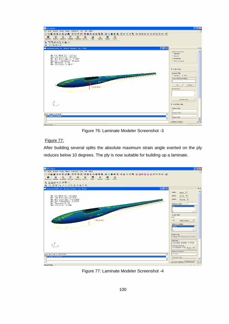
100


Figure 77:

After building several splits the absolute maximum strain angle exerted on the ply

reduces below 10 degrees. The ply is now suitable for building up a laminate.


101

Figure 78:

Left hand side of the body is similarly covered by carbon/epoxy laminate. Excessive

strain angles are reduced by defining splits on necessary regions.

Figure 78: Laminate Modeler Screenshot - 5

Figure 79: Laminate Modeler Screenshot – 6

102

Figure 79:

Since left and right hand sides of the body is covered with plies, a layup can now be

established.

Action: “Create”

Object: “LM_Layup”

Click on Existing LM_Plys and build a layup

Figure 80: Laminate Modeler Screenshot – 7

Figure 80:

24 layers of ply are used to build the composite layup. Each side of the body is

covered with 12 layers. Reference angle shows the orientation of the plies.

Click “OK”

Click “Apply”

Laminate Modeler will associate the properties of composite layup with

corresponding elements. No any additional property definition is needed.

103

APPENDIX C

SOLUTION STEPS OF AN EXAMPLE PROBLEM

In this part, solution steps of a sample problem will be explained. A rigid ball is

projected on a steel plate. In order to preserve simplicity of tutorial the pre-modeled

geometry will be imported into MSC.Patran. Then the geometry will be meshed and

properties will be defined. Boundary conditions and initial velocity of the ball will be

set. Finally, analysis options will be explained and results will be shown.

Opening a new database:

Figure 81: Solution steps, Screenshot -1

Create a new database (Figure 81) and select MSC.Dytran as “Analysis Code”

(Figure 82)

104


Importing geometry:

Geometry is imported by following the steps explained in Appendix A. Imported

geometry has following properties:

Edge length of steel square plate = 1 m

Radius of rigid ball = 0.1 m

After importing the geometry, plate and ball will be seen as in Figure 83.

Figure 83: Solution steps, Screenshot -3 Meshing: (see Figure 84)

Click on “Elements” tab.

Action: “Create”, Object: “Mesh”, Type: “Surface”

105

Figure 84: Solution steps, Screenshot -4 Element Shape: Selects the shape of the element. It can be “QUAD” or “TRIA”

Mesher: “ISOMESH”. For some complex geometry ISO may not be applicable.

“PAVER” should be selected.

Surface List: Select all surfaces (from Surface 1 to Surface 9)

Global Edge Length: The time step size, solution time and precision of solution is

affected by this value. In this example it is selected to be 0.02

Click “APPLY”

Grouping:

Click “Group”, “Create”

New Group Name: “Plate”

Entity Selection: Select all elements on the plate

Click “APPLY”

New Group Name: “Ball”

Entity Selection: Select all elements on the ball

Click “APPLY”

Boundary Conditions and Initial Velocity:

Click “Loads/BCs” tab. (See Figure 85)

Action: “Create”, Object: “Displacement”, Type: “Nodal”

New Set Name: “Fixed”

Click “Input Data” (Figure 86)

106


Translations: “ <0, 0, 0> “, Rotations: “ <0, 0, 0> “ (Fixed Edges)

Click “APPLY”

Click “Select Application Region”

Select: “FEM” (See Figure 87)

Select Nodes: Select all nodes at the edge of the plate

Click “OK”


107


Action: “Create”, Object: “Initial Velocity”, Type: “Nodal”

New Set Name: “Velocity”

Click “Input Data” (See Figure 88)

Transient Velocity: “ <0, 0, -10> “ (10 m/s towards the plate)

Rotational Velocity: “ < > “ (No rotational velocity)

Click “OK”

Figure 88: Solution steps, Screenshot -8 Click “Select Application Region”

Select: “FEM” (See Figure 89)

Application Region: Select all nodes of ball

108

Click “OK”

Click “APPLY”

Figure 89: Solution steps, Screenshot -9 Materials:

Select “Materials” tab (See Figure 90)

Action: “Create”, Object: “Isotropic”, Method: “Manual Input”

Material Name: “rigid_ball”

Click “Input Properties”


109


Constitutive Model: “Rigid (MATRIG)”, Valid for: “Shell” (See Figure 91)

Rigid Body Properties: “Geometry”

Mass: “2”, (2 kg mass for rigid ball)

Click “OK”, Click “APPLY”

Rigid Ball material is created,

Material Name: “steel”

Click “Input Properties” (See Figure 92)

Constitutive Model: “LinElas (DMATEL)”, Element Type: “Membrane”

Density: “7850” (7850 kg/m3 for steel)

Elastic Modulus: “300E9” (300GPa for steel)

Poisson Ratio: “0.3”


Steel material is created.

Now, these materials can be used to define properties for various sections of

geometry. Ball geometry will be defined as “Rigid Ball” and the plate will be defined

as “Steel”.

110

Figure 92: Solution steps, Screenshot -12 Click Properties

Action: “Create”, Object: “2D”, Type: “Shell” (See Figure 93)

Property Set Name: “ball_prop”, click “Input Properties”

Material Name: click “rigid_ball” from materials list

Thickness: “0.05”, Click “OK”


111

Select Application Region: Select all elements of Ball, “Element 1:384”

Click OK, Click “APPLY”. (Ball elements are now associated with rigid material)

Material Name: “Plate”, Click “Input Properties” (See Figure 94)

Material Name: Click “steel” from materials list.

Thickness: “0.005”, (5 mm)

Click “OK”

Click “Select Application Region”, Select all elements of plate, “Element 385:2884”

Click “OK”, Click “APPLY”. (Plate elements are now associated with steel material)


Now, it is necessary to define the geometries that will be in contact during impact.

Since the plate will deform during impact, “contact” should adapt itself accordingly.

Click “Loads/BCs” Action: “Create”, Object: “Contact” (See Figure 95)

Type: “Element Uniform”, Option: “Adaptive Master-Slave Contact”

Click “Select Application Region” (See Figure 96)

Form Type: “Select Tool”, Type: “Master”, Element Type: “2D”, Contact Side: “Both”

Geometry Filter “FEM”. Select all elements of ball, “Element 1:384”

Change Type to “Slave”. Select all elements of plate, “Element 385:2884”


Next step is defining output requests.

112


Figure 96: Solution steps, Screenshot -16 Click “Analysis”

Action: “Analyze”, Object: “Input Deck”, Method: “Translate” (See Figure 97)

Job Name: “sample_prb”, Click “Excecution Controls”

Click “Execution Control Parameters”

End Step: Decides maximum allowable step size. (12000 for this problem)

113

Time Step Size at Start: Defines the initial time step size (1E-6 for this problem)

Minimum Time Step: Defines the allowable minimum step (1E-7 for this problem)

Click “OK”


Click “Execution Controls”

Result Name: “Result” (See Figure 98)

File Type: “Archive”, Result Type: “Element Output”

Chose “Steps for Output” and “Sampling Rate”

0 THRU END BY: Defines the sequence at which the output is written on file

Click “ADD”, Select Groups for Output: “Plate”

Entity Type: “Sublayer Variables”, Click “Inner, Middle, Outer Layer”

Result Type: “EFFST”


MSC.Patran creates a file with “dat” extension and that file can be opened and

processed by MSC.Dytran.

Open MSC.Dytran (See Figure 99)

Select “sample_prb.dat”, set “Memory” to desired level and click “Play” button.

After solution is completed open MSC.Patran for post processing.

114



115

Click “Analysis” (See Figure 100)

Action: “Read Archive File”, Object: “Results”, Method: “Attach”

Click “Select Archive File”, Click “SAMPLE_PRB_PLATE_0.ARC”,

Click “ADD”, Click “APPLY”, Click “APPLY”

MSC.Patran will attach the results.

Figure 100: Solution steps, Screenshot -20 Click “Results”

Action: “Create”, Object: “Quick Plot” (See Figure 101)

Select all solution steps.

Fringe Result: “EFFST”, Deformation Result: “Displacement”

Check: “Animate”, Click: “APPLY”

The result will be shown in animation. Instead of animation a single step can also be

examined. Select the requested step and click “APPLY” without selecting “Animate”.

A single solution step is shown in Figure 102.

116



117

APPENDIX D

EFFECT OF MESH SIZE ON THE ANALYSIS

In Chapter 5 Part 3, fuselage shell model was meshed and covered with carbon

laminate. Meshing was completed with a global mesh length of 10 mm. In this part,

different mesh sizes are examined in order to observe the effect of different mesh

sizes on the analysis. 15 mm, 25 mm and finally 50 mm global edge lengths are

applied and the fuselage is covered with exactly same carbon laminate.

After repeating the analyses it is observed that varying mesh size changes the

maximum stress exerted on the fuselage. The results are tabulated in Table

Table 22: Stress results for different mesh sizes

Global Edge Length (mm)

Number of Elements Effective Maximum

Stress (MPa)

10 2811 353.25

15 1635 433.92

25 541 881.13

50 248 1077.50

As it can be observed, the maximum effective stress increases as the global edge

length increases. Considering the decreasing number of elements it can be said that

bigger mesh results in less accurate results. Therefore, it is reasonable to accept the

smaller element size to be more realistic.

118

APPENDIX E

IMPACT VELOCITY VS. MAXIMUM DEFLECTION

In Chapter 3.6.3 comparison of quasi-static and explicit finite element solutions was

completed and the results were tabulated. In this part, the resolution of the graph is

increased by calculating more data points. As it can be seen in Figure 103, the

amount of error increases almost linearly as the impact velocity is increased.

Figure 103: Impact Velocity (m/s) vs. Maximum Deflection Graph (m)

STRUCTURAL DESIGN, ANALYSIS AND COMPOSITE …etd.lib.metu.edu.tr/upload/12610575/index.pdf ·...

Documents

Transcript of STRUCTURAL DESIGN, ANALYSIS AND COMPOSITE …etd.lib.metu.edu.tr/upload/12610575/index.pdf ·...