Structural Change in U.S. Food Manufacturing,1958–1997

Richard T. RogersDepartment of Resource Economics, 218 Stockbridge Hall,University of Massachusetts, Amherst, MA 01003–9246

ABSTRACT

Public information regarding economic concentration, both aggregate and market, has declinedsince 1982. The Census no longer publishes a concentration report for its Economic Census, whichis done every five years for manufacturing industries. Using purchased data from Census SpecialTabulations, this paper documents advanced aggregate and market concentration in U.S. food andtobacco processing markets. The data are much more useful for studying output markets and fail toprovide much guidance regarding oligopsony issues, which are perceived to be widespread in foodprocessing. In output markets, evidence suggests that a market’s use of media advertising contrib-uted to advanced market concentration prior to 1977, but subsequently concentration has been ris-ing in all industries. Producer good industries have posted the largest increases in concentration asthey narrowed the difference in average concentration between themselves and the group ofadvertising-intensive industries. [EconLit codes: L110, L660] © 2001 John Wiley & Sons, Inc.

This paper examines trends in both aggregate and market concentration within the foodand tobacco processing sector. Despite the simple task, the answers are difficult and ex-pensive. Necessary data either do not exist or are too expensive for a researcher to obtain.The data needs differ depending on whether one assesses oligopsony or oligopoly, asinput markets in food processing are often dramatically more narrowly defined in bothproduct and geographic space than output markets. More public data exist regarding out-put markets, but even so there is less information available now than ten years ago.

The Census no longer publishes a concentration report from its Economic Census andhas discontinued providing any concentration data at the product class level. The productclass data are usually preferred since they use a wherever-made method and a more nar-row market definition (e.g., SIC 20321, canned baby foods, rather than the industry SIC2032, canned specialities, which includes both canned baby foods and canned soup). TheCensus had published concentration reports for manufacturing at both the industry andproduct class levels since 1958. Prior to that, the Congress had the Census prepare specialreports. In 1948, Senator Taft chaired the Joint Committee on the Economic Report andissued a report entitled “Current Gaps in Our Statistical Knowledge,” which asked formore current information on business concentration. In 1957, the Subcommittee on Anti-trust and Monopoly issued its report on “Concentration in American Industry,” whichprovided concentration data for 1954, as well as1935 and 1947. In the letter of transmittalof that report, Joseph O’Mahoney, then chair of the Joint Economic Committee, wrote:

Agribusiness, Vol. 17 (1) 3–32 (2001)© 2001 John Wiley & Sons, Inc.

3

Congress, the administrative agencies, and the general public should be supplied with a continuingbody of information which would show the level or extent of economic concentration in the variousindustries, as well as the changes which have occurred and are constantly taking place. Data of thistype are essential to formulate and implement policies and programs in this area. . . . It is felt thatpublication of a large body of authoritative data in a field in which such data have been notablylacking for so long will serve a useful and timely public purpose in achieving a better insight intothe structure of our industrial economy. (p. III)

Congress needs to reissue those appeals as the Census has dramatically reduced theamount and timeliness of its concentration data. The last concentration report was for the1987 Census and it excluded a product class report, reporting concentration only for in-dustries. In 1992 the Census did not issue a written concentration report but posted in-dustry concentration data for manufacturing on its website. With support from the EconomicResearch Service of the U.S. Department of Agriculture, the Food Marketing Policy Cen-ter at the University of Connecticut and the Food Systems Research Group at the Uni-versity of Wisconsin, we asked Census for a special tabulation to provide product classconcentration data for 1987, 1992, and 1997. Unfortunately, budget problems, time pres-sures, and resource constraints intervened, and we managed to secure only the productclass concentration data for 1987 and 1992 (the data are available in electronic form fromthe author).

1. OVERALL INDUSTRIALIZATION AND CONSOLIDATION

The American food system continues to consolidate and industrialize as consumers splin-ter into more segments and technology allows catering to the diversity of demands whileretaining large economies of scale. Economic markets can be incredibly efficient, butmany traditional agricultural markets are being replaced by vertical integration, strategicalliances, and contracts. Little to no data exist on these private transactions; hence eco-nomic assessments are difficult (see, e.g., Dimitri, 1999) and require industry coopera-tion, either willingly or forced by legal means.

Economists understand the benefits of these non-market transactions, as much of theindustrialization has featured improved information, tailored inputs, and reduced cost ofproduction and processing. There are also costs: As more product volume moves throughnon-market methods the less is known about true product values as key economic infor-mation summarized by price becomes more difficult to discover. Consumer concerns arisefrom whether there will be sufficient competition to force such efficiencies to be passedon as lower prices, and rural communities wrestle with major issues resulting from fac-tory farms that reduce the number of family farms and add to environmental concerns.Even producers who entered these contracts worry whether they will receive fair pricesfor their products once the marketplace is removed or diminished.

All stages of the vertical system are becoming more concentrated as larger operationsincrease their size. At the same time, there is an enhanced bimodal distribution as thelarger firms get larger and the number of smaller firms increases. The processing stagehas the fewest number of companies in the vertical food system, but the processor/foodmanufacturer is often considered the most powerful, influential firm in the system—themarketing channel leader. These are the food firms the world knows by name: PhilipMorris, Coca-Cola, Cargill, Kelloggs, among others. About 80% of all raw domestic foodproducts pass through this stage, with only produce and eggs avoiding processing be-

4 ROGERS

cause they only require minimal market preparation services such as cleaning, sorting,and packaging (Connor, Rogers, Marion, & Mueller, 1985).

Food processors’ location decisions involve a calculated tradeoff between processingcosts, including input costs, and the costs of delivering their finished products to con-sumers. Over time, with modern transportation and preservation technologies, the bal-ance has shifted to locating where the inputs are produced rather than where the peoplelive. California is in the unique situation of being both the number-one farm state and thenumber-one food processing state by far (Rogers, 2000). States such as Nebraska andKansas, which rank 4th and 5th in farm production value, rank 24th and 27th, respectively,in processing. Overall there is a strong association between agricultural production rankand food processing rank, with a simple correlation coefficient of .75. In certain crops,such as in wine or broilers, it is even more pronounced.

Food and tobacco processing saw the most dramatic consolidation in the twentiethcentury, as merger patterns followed the four great merger movements of the generaleconomy. The first major merger wave occurred around the turn of the century and cre-ated some of the famous trusts that antitrust legislation was supposed to prevent (Connor& Geithman, 1988). For example, American Tobacco and General Mills were formedduring this merger wave. The next wave came during the 1920s, when companies such asGeneral Foods were being formed through merger. The third merger wave, in the 1960s,was characterized by amazing conglomerates being formed as unrelated firms sought man-agement synergies. The fourth merger movement, in the late 1970s and 1980s, was a wildperiod of leveraged buyouts and hostile takeovers often funded with questionable finan-cial instruments. Food companies were at the forefront of these mergers with record-setting deals such as the $25-million leveraged buyout of RJR Nabisco. The largest foodand tobacco processor, Philip Morris Cos., is essentially a case history in a merger-builtbusiness. Starting from its strong position in cigarettes, Philip Morris purchased suchalready huge companies as Miller Brewing, General Foods (who already had bought Os-car Mayer), and Kraft Foods. Currently, the company is in negotiations to purchase NabiscoFoods.

It appears that we are in the midst of a fifth merger wave, and again the food businessesare major players. Most of the food-related mergers involve food processing firms, in-cluding some the largest mergers in history, but increasingly mergers in retailing, foodservice, and wholesaling are commonplace. Some of the failures of the previous mergerwave are being undone as firms now seek to buy only parts of other firms as they selec-tively add and subtract from their portfolio of brands. Others merely purchase firms whosebrands fit well with their current offerings. This current merger wave is more horizontalin nature as processing firms seek merger partners among current rivals. Gone are thewild conglomerate mergers, as firms now seek to consolidate their hold on leading posi-tions in markets where they currently hold a strong position. Some economists have be-come concerned about the growing concentration and march toward oligopoly in almostevery market.

The largest food processors among the roughly 16,000 companies are huge, both inabsolute terms and relative to the others. The 100 largest food and tobacco processorsaccounted for about 75% of the value-added in 1997 (Figure 1), almost doubling theirshare since 1954. The top 100 is itself skewed toward the very large, with the top 20 firmsaccounting for over 50% of total value-added in 1997, more than doubling its 1967 share(Figure 2). The remaining 80 firms among the top 100 actually lost share over the last 30years. The sector is best described by a big–small model, where extremely large firms

STRUCTURAL CHANGE IN U.S. FOOD MANUFACTURING 5

control leading positions in most markets, and smaller companies, including startups,operate in a competitive fringe trying to serve a particular market niche or develop a newidea.

The dramatic size of the top 20 companies is seen from the recently completed 1992special tabulation (Tables 1 and 2). These firms are multi-plant operations, averaging 56plants per firm. The number of establishments per firm declines with each size class, untilthe firms ranked lower than the top 500 had an average of 1.1 establishments per firm.The payroll of the top 20 in 1992 was about the same as the entire payroll for the 15,652firms ranked lower than the top 500. The leading 20 food and tobacco companies are alsothe most heavily involved in the highest value-added products, with a ratio of value-added to shipments of .54 in 1992, much higher than the .41 that the next 30 largest firmshad. The ratio for the firms ranked 51 to 500 was about .35, still higher than the .316 forthose firms ranked over 500.

The previous figures refer to overall size, or aggregate concentration, but market per-formance hinges more directly on market concentration. Market power is what enables afirm to enhance prices to buyers, to extract price reductions from its product suppliers,and to subdue rivals. Although market definition is a complex task, it has been roughly

Figure 1 Aggregate concentration among the 100 largest food manufacturing companies, Censusyears 1954–1997.

6 ROGERS

approximated by the Census four-digit industry group, the 4-digit SIC, at least on theoutput side of the market in numerous empirical studies. The food and tobacco process-ing sector had 53 such industries in 1992, many of which remain too broadly defined—certainly so on the input side as substitution opportunities are much greater in consumptionthan production. Although there are no monopolies, and several industries are whateconomists call workably competitive (where the four largest firms have a combinedmarket share of 40% or less), most have become oligopolies (Table 3). In oligopolies,firms get some of the advantages of market power without government regulation thatwould come if they were monopolies (Zachary, 1999). Over time most of these 4-digitindustries have lost companies, averaging a 25.5% reduction in company counts, andhave increased in concentration as measured by the four-firm concentration ratio, CR4,which increased on average from 43.9 in 1967 to 53.3 in 1992, the last year data areavailable.

2. OLIGOPSONY IN FOOD PROCESSING

Forty years ago, Robert Lanzillotti presented a paper at the meeting of the AmericanAgricultural Economics Association in a session titled “Market Power and the Farm Prob-

Figure 2 Increasing dominance by the top 20 among the 100 largest food and manufacturingcompanies, Census years 1967–1997.

STRUCTURAL CHANGE IN U.S. FOOD MANUFACTURING 7

lem” (Lanzillotti, 1960). Lanzillotti assembled data for 51 industries (28 were food andtobacco processing industries) that were relevant to farmers, both on the input and outputsides. His data led him to conclude: “The foregoing statistics on the structural character-istics and growth path of the food processing and agricultural supply industries are fairlystrong circumstantial evidence of high and growing market power in the economic sense”(p. 1239). Since companies had higher shares than plants, he concluded that it was nottechnical efficiencies that were driving firms to ever larger shares. He gave the trends inmergers and acquisitions to further sound the alarm that “Farmers, as sellers, have foundthemselves at the mercy of oligopsonies, collusion, and monopsony” (p. 1240).

Lanzillotti could not have been pleased by the major consolidations that have takenplace since 1954, but they suggest that his main conclusion applies even more so today:“. . . the structural features of agriculture, i.e., the size-distribution of farms, producthomogeneity, level of managerial skill, exit barriers, demand-supply elasticities, etc., are

TABLE 1. Aggregate Concentration, Measured by Value-Added, in Food and TobaccoProcessing, 1992

CompanyRankingGroup

Numberof

Companies

Numberof

Estabs

Estabsper

Company

Value-Added

(Millions $)

Percent ofValue-Added

Ratioof

VA to VS

All Companies 16,152 20,912 1.3 184,467 100.0% 41.7%

1–20 20 1,121 56.1 81,255 44.0% 53.6%21–50 30 755 25.2 30,583 16.6% 41.1%51–100 50 686 13.7 15,128 8.2% 35.1%101–200 100 734 7.3 13,087 7.1% 35.0%201–500 300 1,052 3.5 15,334 8.3% 35.2%501 and higher 15,652 16,564 1.1 29,080 15.8% 31.6%

Notes.Companies were ranked by value-added in food and tobacco processing. Estabs5 establishments, VA5value added, VS5 value of shipments.Source.Special tabulation from the Census of Manufactures, U.S. Census Bureau. Prepared under the super-vision of Patrick Duck of the Census Bureau and Richard Rogers of the University of Massachusetts. Purchasedby the Food Marketing Policy Center, University of Connecticut.

TABLE 2. Aggregate Concentration, Measured by Employment, Payroll,and Value of Shipments, in Food and Tobacco Processing, 1992

CompanyRankingGroup

TotalEmployment

(number)

Percentageof Total

Employment

TotalPayroll

(millions $)

Percentageof TotalPayroll

Value ofShipments(millions $)

Percentageof Total

Shipments

All Companies 1,540,787 100.0% 38,296 100.0% 442,161 100.0%

1–20 340,639 22.1% 10,456 27.3% 151,690 34.3%21–50 216,107 14.0% 5,524 14.4% 74,438 16.8%51–100 151,735 9.8% 3,610 9.4% 43,090 9.7%101–200 138,611 9.0% 3,302 8.6% 37,406 8.5%201–500 195,384 12.7% 4,719 12.3% 43,584 9.9%501 and higher 498,311 32.3% 10,686 27.9% 91,952 20.8%

Note.Same as Table 1.Source.Same as Table 1.

8 ROGERS

conducive to an inferior bargaining position for farmers vis-à-vis both buyers and sup-pliers” (p. 1243). He saw two approaches to offset this imbalance: “a) to build counter-vailing power through direct or indirect government action or special additional antitrustimmunities for agriculture, and (b) to dissolve or lessen the market power of groups towhom the farmer sells or from whom he buys” (p. 1246). He clearly favored the secondapproach as he disliked “the further cartelization of agriculture,” and he thought the firstapproach would not provide a suitable solution “because it attempts to replace the ‘in-visible hand’ of Adam Smith with the ‘invisible fist’ of government” (p. 1246). Cooper-atives were a common farmer response to weak bargaining positions but he resisted grantingthem more favorable treatment because “greater insulation of cooperatives’activities fromantitrust statues, for example, serve no general social ends and are not economically jus-tified” (p. 1246). He preferred “More vigorous antitrust policy, [because] while slow,offers the basic and most effective approach to redressing market power” (p. 1246). Clearly,over the 40 years since he wrote his conclusions, farmers have had more success withinstitutions designed to limit the power of buyers than from an aggressive antitrust policyto preserve competitive markets in which farmers could sell. Cooperatives, bargainingassociations, marketing orders, and even electronic auctions have been used to improvefarmers’ economic power imbalance with buyers.

The structural data on food and tobacco processing industries given in Table 3 fail toprovide the necessary information to study oligopsony. In addition to problems with thegeographic scope of an industry, the Census 4-digit industry data often are too broad toreflect a properly defined market on the basis of product scope. Of the 53 industries givenin Table 3, several are well-defined product markets (e.g., butter or malt beverages), butothers are much too broad (e.g., canned fruits and vegetables or dehydrated fruits andvegetables) and essentially all are too broad for input markets. As Rogers and Sexton(1994) noted, “although there were 81 firms in canned fruits in 1987, only 5 and 11 pro-cessed cranberries and olives, respectively. Thus, whereas canned fruits may represent arelevant output market class, it is far too broad for analysis of competition in the rawproduct markets because the vast majority of fruit processors do not compete, for exam-ple, for olives or for cranberries” (p. 1144). Needed data are not readily available, and thesituation is getting worse as public information diminishes. In addition, larger firms arereconsidering the strategic tradeoffs of sharing proprietary firm data with industry-widedata collection efforts. The strategic value of asymmetrically held information increasesas a firm’s market share increases.

Economists have not given sufficient attention to oligopsony issues in part because ofdata limitations. As Scherer and Ross (1990) state, “A quantitative picture of how muchbuyer concentration exists is difficult to secure, for there are no statistical series analo-gous to the abundant data on seller concentration. An impressionistic view suggests thatconcentration on the buyers’ side is generally more modest than concentration on thesellers’ side, although appreciable pockets of monopsony or oligopsony power . . . can befound” (p. 517). Agriculture is definitely one of those pockets. Rogers and Sexton exam-ined the unique characteristics of agricultural markets (bulky and/or perishable product,specialized processing needs with little to no input substitution, specialized investmentsin sunk assets, and cooperatives, bargaining associations, or other institutions of sellerpower exist or could exist) and argue for agricultural economists to recognize the dra-matic influence these unique characteristics have on assessments of market power.

To study buyer concentration is to study vertical marketing systems, or what has beencalled subsector analysis. Agricultural economists have a rich tradition of doing such

STRUCTURAL CHANGE IN U.S. FOOD MANUFACTURING 9

TAB

LE

3.

Co

nce

ntr

atio

nin

Fo

od

an

dTo

ba

cco

Pro

cess

ing

Ind

ust

rie

s,1

96

7–1

99

2

Co

nce

ntr

atio

n-C

R4

Nu

mb

er

of

Co

mp

an

ies

SIC

Na

me

19

67

19

87

19

92C

ha

ng

e6

7–8

7C

ha

ng

e8

7–9

21

96

71

98

71

99

2

%C

ha

ng

e6

7–8

7

%C

ha

ng

e8

7–9

2VA/V

S

Ag

Inp

ut

Sh

are

Co

-op

VS

Sh

are

201

21

All

foo

d&

tob

acc

op

rod

uct

s(a

)5

16

66

91

53

26

95

81

57

90

16

15

224

1.4

2.3

47

.2—

5.4

20

11

Me

at

pa

ckin

gp

lan

tp

rod

uct

s2

63

25

06

18

25

29

13

28

12

96

24

7.5

22

.41

1.6

75

.90

.12

01

3S

au

sag

es

&p

rep

are

dm

ea

ts1

52

62

51

12

11

29

41

20

71

12

82

6.7

26

.52

6.9

0.0

0.1

20

15

Po

ultr

ya

nd

eg

gp

roce

ssin

g1

52

83

41

36

70

92

84

37

32

59

.93

1.3

27

.66

8.5

5.0

20

21

Bu

tte

r1

54

04

92

59

51

04

43

129

1.4

22

9.5

9.4

19

.16

2.8

20

22

Ch

ee

se,

na

tura

lan

dp

roce

sse

d4

44

34

22

12

18

91

50

84

18

24

3.0

21

7.7

20

.24

7.2

23

.42

02

3C

on

de

nse

da

nd

eva

po

rate

dm

ilk4

14

54

34

22

17

91

24

15

32

30

.72

3.4

40

.83

6.1

27

.12

02

4Ic

ecr

ea

ma

nd

ice

s3

32

52

42

82

17

13

46

94

11

23

4.2

21

2.4

32

.47

.26

.02

02

6F

luid

milk

22

21

22

21

12

98

86

52

52

52

78

.22

19

.52

6.4

56

.41

7.2

20

32

Ca

nn

ed

spe

cia

litie

s6

95

96

92

10

10

15

01

83

20

02

2.0

9.3

49

.65

.70

.52

03

3C

an

ne

dfr

uits

an

dve

ge

tab

les

22

29

27

72

29

30

46

25

02

25

0.3

8.7

45

.82

8.0

13

.72

03

4D

eh

yd.

fru

its,

veg

eta

ble

s,so

up

s3

23

93

97

01

34

10

71

24

22

0.1

15

.95

1.2

15

.01

4.2

20

35

Pic

kle

s,sa

uce

s,sa

lad

dre

ssin

gs

33

43

41

10

22

47

93

44

33

22

28

.22

3.5

50

.41

0.3

1.8

20

37

Fro

zen

fru

itsa

nd

veg

eta

ble

s(b

)3

12

82

23

19

41

82

42

.62

6.2

45

.24

6.2

8.4

20

38

Fro

zen

spe

cia

ltie

s(b

)4

34

05

23

24

43

08

23

7.1

26

.24

9.9

5.9

0.2

20

41

Flo

ur

&o

the

rg

rain

mill

pro

du

cts

30

44

56

14

12

43

82

37

23

024

5.9

23

.02

6.8

70

.11

.02

04

3C

ere

alb

rea

kfa

stfo

od

s8

88

78

52

12

23

03

34

21

0.0

27

.37

4.7

8.7

0.0

20

44

Mill

ed

rice

an

db

ypro

du

cts

45

56

50

11

26

54

48

44

21

1.1

28

.33

8.0

88

.24

4.5

20

45

Pre

p.

flou

rm

ixe

s&

refr

.d

ou

gh

s6

34

33

92

20

24

12

61

20

15

62

4.8

30

.04

8.7

0.0

0.0

20

46

We

tco

rnm

illin

g6

87

47

36

21

32

31

28

23

.12

9.7

43

.35

3.3

0.0

20

47

Do

g,

cat,

an

do

the

rp

et

foo

d4

66

15

81

52

31

30

10

22

11

.62

21

.55

4.1

7.0

0.2

20

48

Pre

pa

red

fee

ds,

n.e

.c.,

(b)

(e)

22

20

23

22

31

18

21

16

12

25

.12

1.8

22

.71

6.0

4.2

20

51

Bre

ad

,ca

ke,

&re

late

dp

rod

uct

s2

63

43

48

03

44

51

94

82

18

02

43

.51

1.9

64

.90

.00

.22

05

2C

oo

kie

sa

nd

cra

cke

rs5

95

85

62

12

22

86

31

63

74

10

.51

8.4

65

.00

.00

.02

05

3F

roze

nb

ake

ryp

rod

uct

s5

94

52

14

10

31

60

55

.35

1.5

0.0

0.0

20

61

Su

ga

rca

ne

mill

pro

du

cts

43

48

52

54

61

31

372

49

.21

9.4

40

.78

1.3

10

.72

06

2R

efin

ed

can

esu

ga

r5

98

78

52

82

22

21

41

22

36

.42

14

.31

8.1

0.0

15

.52

06

3R

efin

ed

be

et

sug

ar

66

72

71

62

11

51

41

32

6.7

27

.13

3.5

75

.32

9.3

20

64

Ca

nd

y&

con

fect

ion

ary

(c)

45

45

07

05

55

.01

.90

.72

06

6C

ho

cola

tea

nd

coco

ap

rod

uct

s6

97

56

17

31

46

21

5.6

46

.60

.3d

0.0

20

67

Ch

ew

ing

gu

m(c

)8

69

69

61

00

19

882

57

.90

.06

8.8

0.0

0.0

10 ROGERS

20

68

Nu

ts&

see

ds

43

42

21

79

10

22

9.1

39

.83

5.5

25

.92

07

4C

ott

on

see

do

ilm

illp

rod

uct

s4

24

36

21

19

91

31

222

65

.92

29

.02

2.7

67

.61

6.0

20

75

So

ybe

an

oil

mill

pro

du

cts

55

71

71

16

06

04

74

222

1.7

21

0.6

11

.17

6.0

16

.82

07

6V

eg

eta

ble

oil

mill

pro

du

cts,

n.e

.c.

56

74

89

18

15

34

20

1824

1.2

21

0.0

19

.27

0.8

4.3

20

77

An

ima

lan

dm

ari

ne

fats

an

do

ils2

83

53

77

24

77

19

41

5925

9.3

21

8.0

42

.70

.01

.52

07

9S

ho

rte

nin

ga

nd

coo

kin

go

ils4

34

53

52

21

06

36

77

26

.37

.53

0.4

0.0

4.3

20

82

Ma

ltb

eve

rag

es

40

87

90

47

31

25

10

11

602

19

.25

8.4

53

.51

.90

.02

08

3M

alt

an

dm

alt

byp

rod

uct

s3

96

46

52

51

32

15

162

53

.16

.72

8.9

85

.40

.02

08

4W

ine

s,b

ran

dy,

an

db

ran

dy

spir

its4

83

75

42

11

17

17

54

69

51

41

68

.09

.64

3.0

27

.02

.52

08

5D

istil

led

liqu

or,

exc

ep

tb

ran

dy

54

53

62

21

97

04

84

32

31

.42

10

.45

9.5

2.0

0.1

20

86

Bo

ttle

da

nd

can

ne

dso

ftd

rin

ks1

33

03

71

77

30

57

84

66

37

27

2.3

22

4.7

38

.50

.04

.12

08

7F

lavo

rin

ge

xtra

cts

&sy

rup

sn

.e.c

.6

76

56

92

24

40

12

45

26

42

38

.97

.87

0.6

0.0

0.3

20

91

Ca

nn

ed

&cu

red

sea

foo

din

cso

up

44

26

29

21

83

26

81

53

14

42

42

.92

5.9

36

.90

.0d

0.0

20

92

Fre

sho

rfr

oze

np

ack

ag

ed

fish

26

18

19

28

15

79

60

03

.62

6.8

0.0

d0

.02

09

5R

oa

ste

dco

ffee

53

66

66

13

02

06

11

01

342

46

.62

1.8

40

.50

.0d

0.6

20

96

Po

tato

chip

sa

nd

sim

ilar

pro

du

cts

41

62

70

21

82

77

33

32

0.2

65

.51

9.4

0.0

20

97

Ma

nu

fact

ure

dic

e3

31

92

42

14

56

88

50

35

13

22

6.9

2.0

70

.00

.00

.02

09

8M

aca

ron

ian

dsp

ag

he

tti

34

73

78

39

51

90

19

61

82

3.22

7.1

58

.60

.00

.02

09

9F

oo

dp

rep

ara

tion

s,n

.e.c

.2

32

62

23

24

18

24

15

10

16

44

21

7.2

8.9

52

.48

.30

.62

11

1C

iga

rett

es

81

92

93

11

18

98

12

.521

1.1

74

.72

.30

.02

12

1C

iga

rs5

97

37

41

41

12

61

62

528

7.3

56

.35

5.5

4.7

0.0

21

31

Ch

ew

ing

,sm

oki

ng

tob

acc

o,

snu

ff5

18

58

73

42

41

23

2324

3.9

0.0

71

.14

.20

.02

14

1To

ba

cco

ste

mm

ing

an

dre

dry

ing

63

66

72

36

54

62

32

14

.824

8.4

19

.04

9.5

0.0

me

an

sfo

rS

IC2

0–2

14

3.9

51

.15

3.3

7.5

2.1

22

5.5

3.0

42

.82

4.1

6.9

No

tes.

CR

4s

are

fro

m4

-dig

itin

du

stry

da

ta,

wh

ere

ava

ilab

le,

els

e4

-dig

itp

rod

uct

cla

ssd

ata

fro

mR

og

ers

.(a

):F

or

SIC

201

21

the

con

cen

tra

tion

da

taa

reth

ep

erc

en

tag

eo

fth

ese

cto

r’sva

lue

-ad

de

dh

eld

by

the

top

10

0fo

od

an

dto

ba

cco

com

pa

nie

s.(b

):T

he

cha

ng

es

are

fro

m1

97

2,

no

t1

96

7.

(c):

In1

99

2,

SIC

20

67

,C

he

win

gG

um

,w

as

com

bin

ed

with

SIC

20

64

.Th

e1

99

2d

ata

for

SIC

20

67

are

est

ima

ted

by

Ro

ge

rs.

(d):

Co

coa

,co

ffee

,a

nd

fish

inp

uts

we

reig

no

red

.(e

):1

96

7C

R4

ise

stim

ate

d.

Wh

ere

:VA/V

Sis

the

ratio

of

valu

e-a

dd

ed

toth

eva

lue

-of-

ship

me

nts

,p

erc

en

t,1

98

7d

ata

.A

gIn

pu

tsh

are

isth

ep

erc

en

tag

eo

fto

talc

ost

of

ma

teri

als

acc

ou

nte

dfo

rb

ya

gri

cultu

rali

np

uts

,1

98

7d

ata

.C

o-o

pV

SS

ha

reis

the

19

87

est

ima

ted

pe

rce

nta

ge

of

valu

e-o

f-sh

ipm

en

tsa

cco

un

ted

for

by

the

10

0la

rge

sta

gri

cultu

ralm

ark

etin

gco

op

era

tive

s.S

ou

rce.

Ce

nsu

so

fM

an

ufa

ctu

rin

g,

pre

pa

red

by

Ric

ha

rdT.

Ro

ge

rs,

De

pa

rtm

en

to

fR

eso

urc

eE

con

om

ics,

UM

ass

,Am

he

rst,

MA

01

00

3.

STRUCTURAL CHANGE IN U.S. FOOD MANUFACTURING 11

studies, usually as case studies of a particular agricultural commodity (see, e.g., Marion,1986, chap. 3). The data requirements of these studies are dramatic and offer a uniqueinsight into the how farmers, intermediaries, institutions, processors, distributors, andretailers accomplish the task of moving an agricultural commodity from production toconsumption. Over time the profession has produced a vast array of such studies, but theytend to become outdated and few unambiguous performance conclusions can be drawnfrom them. Nevertheless, these studies provide one of the best vantage points to examineconcerns over buyer concentration as they usually track product flows from farmer to allfinal consumption points and often give concentration information on the number andsize distribution of buyers along the way.

These vertical studies must address the other critical issue involved in buyer (and seller)concentration, namely, market definition. Both product and geographic scopes must beconsidered, and the importance of spatial economics becomes apparent. It is not uncom-mon for a commodity to move from a local geographic market at the original procure-ment stage (grain delivered to the rural elevator) to a global market definition at the laterstages of production (grain exports). Merely an examination of the current economic play-ers and the regional flows of products is not sufficient, as economists are concerned aboutsupply responses induced by price changes. The merger guidelines use a theoretical no-tion in which a hypothetical monopolist (monopsonist) would impose a “small but sig-nificant and nontransitory” price increase. In practice, a 5% increase was often used butthe 1992 guidelines backed away from stating any specific amount.

The few general economists who have attempted an empirical study of buyer concen-tration (e.g., Lustgarten, 1975) have not addressed these issues. They usually estimatebuyer concentration from the level of national seller concentration of the manufacturingindustries. When a manufacturing industry buys the supplying industry’s total output,then the seller concentration does provide the degree of buyer concentration if, and onlyif, the procurement market is national as well. This is not the case in much of agriculture.Also, seldom does a manufacturing industry buy the entire supplying industry’s output,although this is common in agriculture. When an industry is not the exclusive user of asupplying industry’s output, then the national seller concentration ratios are weighted bythe amount these industries buy from each of the supplying industries. The weights aretaken from the national input–output tables. Another major data problem emerges here inthat these industry definitions are much too broad, reflecting less exclusive use than ac-tually exists. When one examines the 1982 Input–Output tables to discover the extent ofthe total supply of an agricultural commodity (e.g., processing tomatoes) used by a foodprocessing industry (say, canned fruits and vegetables), one finds that all agriculturalvegetables are combined into a single industry.

The data problems alone limit the number of empirical studies. Despite the limited num-ber of studies, some information on buyer concentration faced by farmers is publicly avail-able and is suggestive of oligopsony. Although far from conclusive, firm counts andconcentration data remain useful as a first step in determining where additional informationis required. Few market power problems arise where numerous, similarly sized firms com-pete. However, even a small number of buyers (sellers) is not sufficient to conclude that mar-ket power exists. Conditions of entry, and even just the credible threat of entry, can restrainany attempts to profit from any market power that might be possible in the short run. Nev-ertheless, concentrationdatacanbeused tohighlightpotential areaswarranting furtherstudy.

The Census of Manufacturers provides most of the public data used by economistsstudying the manufacturing sector, including food and tobacco processing. In addition,

12 ROGERS

much detailed data on the livestock related industries are available from U.S. Depart-ment of Agriculture. The narrowest Census data definition is the 7-digit product level,and at this level the only relevant data are the number of companies that had value-of-shipments of at least $100,000 for that product in the year. These data show far fewercompanies at the product level than the product class level. Consider canned fruits,which had 76 firms in 1992 and a CR4 of 47. In particular, for fruits like apricots,cranberries, peaches, pineapples, and olives there were less than 10 companies in eachof them and all experienced a decrease in the number of firms from 1992 to 1997 (ex-cept cranberries, which had three firms in both years). Such product detail is necessaryfor studying agricultural markets, yet it still remains national data and hence fails toaddress spatial monopsony concerns.

The Census provides industry (4-digit) data at the state level, and even at the countylevel, but the extent of the data falls off dramatically from the national level to the stateand county levels. For example, the state level does not give company counts, only es-tablishment counts. In addition, there are no data on size distribution of the establish-ments other than a separate count for those establishments with more than 20 employees.

Although Table 3 is woefully inadequate for questions related to oligopsony, it doessuggest that farmers selling to the processing industries face fewer and more dominantfirms buying their output. Decreases in firm numbers and increases in concentration ra-tios were common over time. The wine industry (SIC 2084) was the only industry toshow a large increase in the number of firms (1339), but the industry CR4 rose from1987 to 1992. This is the only industry that gave farmers substantially more buyers in1992 than existed in 1967. The cookies and crackers industry did increase by 88 firmswith a small decrease in its CR4, but this is not an industry of direct importance to farm-ers. The variable, ag input share, measures the extent the industry relies on U.S. farmoutput for its input—ranging from 0% for no U.S. agricultural inputs are purchased bythe processing industry to 88% in the milled rice industry.1

Overall, there is an inverse correlation between change in company numbers and con-centration change. Only in a few cases can a positive relationship be found. The mostdramatic case was in the beer industry where company counts increased, yet its CR4jumped by 50 percentage points. The end result was that farmers and consumers facemore concentrated processing industries; the only other remedy available to them was toseek institutional arrangements to offset any power imbalance. Cooperatives allow farm-ers to integrate forward into processing and avoid having to sell to a firm that has mo-nopsonistic power. The immense size of processors has always concerned farmers whofeared the processors would exploit their bargaining power and pay farmers less than fairmarket value for their crops. Such fears led to agricultural cooperatives and the Capper–Volstead Act of 1922. Both economic theory (e.g., Cotterill, 1997) and empirical studies(e.g., Rogers & Petraglia, 1994) conclude that open-membership cooperatives can negatemarket power imperfections and hence benefit both farmers and consumers.

In Table 3 the share of an industry’s shipments controlled for by the 100 largest coop-eratives in 1987 ranges from a high of 63% in the butter industry to several industrieswithout any cooperatives, and averages 5.4% for all of food and tobacco processing. Farm-ers selling through their marketing cooperative do not worry about concentration in theprocessing market. The second highest cooperative share was in rice milling (44%), andseveral more industries had a cooperative share exceeding 10%, especially in the dairy

1In the case of coffee, it was assigned 0% even though a small amount of coffee is grown in Hawaii.

STRUCTURAL CHANGE IN U.S. FOOD MANUFACTURING 13

industries. Much of the cooperative involvement in forward integration of their farmermembers output is lost when just food processing industries are examined because coop-eratives have a major presence in the first-handler markets that the Census classifies out-side of processing. For example, although there were no cooperatives with establishmentsprimary to meatpacking in 1987, they did account for 8.9% of all buying and marketingof livestock, including cattle, hogs, and sheep (SIC 5154). Similarly, only one coopera-tive had an establishment primary to flour milling and the cooperative share was just 1%,but the cooperative share of buying and marketing grain, dry beans, and soybeans (SIC5153) including country grain elevators was 4.2%.

There is a statistically significant positive correlation between how important an in-dustry is to farmers, as measured by ag input share, and the percentage share held bycooperatives. Indeed, in a simple regression model explaining percentage share held bythe 100 largest cooperatives, the importance of the farm input is positive and significant,and the ratio of an industry’s value-added to value-of-shipments is negative and signifi-cant. However, history does matter and in several industries where one would expect astrong cooperative presence, none was found. Whereas in almost all of the dairy indus-tries cooperatives have a large presence, none was found in the tobacco stemming andredrying industry. This industry has nearly 50% of its cost of materials attributed to to-bacco but no cooperatives were present. Campbell (1990) provides a history of an at-tempt by tobacco growers to form a cooperative to challenge the “Tobacco Trust” puttogether by the American Tobacco Company (ATC) around the turn of the century. Thetobacco farmers were being offered prices below the cost of production as there were nobuyers competing with ATC or its purchasing agents. The cooperative organized nearly athird of the growers in the Kentucky/Tennessee region known as the “black patch” by1908 but failed two years later. The failure was attributed to poor organization and leader-ship and attacks from ATC.

Most researchers have had to abandon Census data for studying oligopsony. Within thelivestock industries researchers have used either the U.S. Department of Agriculture datafrom inspection records or from Packers and Stockyards. Others seeking even more dis-aggregated data, or studying other industries, have turned to industry-supplied data, ei-ther provided by industry cooperation or authorized by governmental agencies chargedwith oversight responsibilities. The researchers need for detailed firm data is seldom re-alized and most studies must make do with less than ideal data. The meat industries havebeen the subject of the most recent studies and even here, where the data are more de-tailed and available, the research has reached inconclusive results.

3.1 Oligopoly in Food Processing

Concentration in food processing markets is of interest to both farmers and consumers.The analysis of concentration data in the remainder of this paper focuses on output mar-kets and fails to provide much guidance for oligopsony issues, other than by providing acrude measure: If output markets are concentrated, then the agricultural input markets arelikely to be even more so. The available concentration data limit us to examining thefour-firm concentration ratio as it is the most accepted and traditional measure of marketconcentration. The Hirshman–Herfindalh, the H-index, is often preferred by economists,usually for its nice algebraic properties in theoretical derivations, but the two measuresare highly correlated.

14 ROGERS

3.2 Sunk Costs and Market Structure

Sutton (1991) attempted to close the gap between the inadequate Structure-Conduct-Performance (S-C-P) paradigm and the game theory approach to the determination ofindustrial structure. The S-C-P school had been discredited as simplistic and ignoringfeedback from performance and conduct to structure. The game theorists gave us manymodels but few robust conclusions as the game’s details led to numerous outcomes, whichdepended on the model’s specifications. Sutton’s approach was to seek broad conclusionswithout sacrificing theoretical rigor or prior empirical regularities found in the literature.Briefly, his model is a two-stage game, where in stage 1 a firm decides whether to enterthe market. If a firm enters it must pay a sunk cost,s, and then in stage 2 the firm facessome form of price competition that can be either soft (price exceeds marginal cost) orhard (price at marginal cost). The sunk costs can either be exogenous, as in the casewhere a firm must acknowledge current scale economies and build or buy a plant of min-imum efficient size. This cost must be borne by all entrants and is exogenously deter-mined by technology. Additionally, firms can choose to invest in advertising to increaseconsumers’ willingness to pay for their products; hence this sunk cost is endogenouslydetermined as firms make this choice: to advertise or not to advertise.

This distinction between the sunk costs being exogenously or endogenously deter-mined is central to Sutton’s theory in explaining industry concentration. In the food in-dustries, the use of advertising is critical to this classification as those industries thatproduce homogeneous goods (e.g., sugar) unaided by consumer advertising face only theexogenous sunk cost of having a plant of minimum efficient size, whereas in industrieswhere advertising is used (e.g., breakfast cereals) firms must choose a level of advertis-ing and hence face an endogenous sunk cost.

Sutton (1991) lays out his full theory in Chapters 2 and 3 of his book. In Chapters 4and 5 he tests his general conclusions using data from the six largest Western econo-mies, 20 food industries, and a reference year of 1986 (although much of the data arefrom the mid-1970s due to availability). To his credit he is very careful in selectingindustries that allow comparisons across the six countries. He is equally deliberate inhis choice of empirical measures for his theoretical variables. He uses the CR4 for hisconcentration measure, although he also uses a logit transformation on CR4 to addressthe limits problem. For the setup cost,s, the minimal sunk cost all firms must pay toenter an industry, he uses the median plant size relative to total market size, called MESin the literature (see Connor et al., 1985, or Sutton, 1991, pp. 94–99; Sutton takes hisMES estimates from Connor et al.). Sutton is well aware of the limitations of this mea-sure, including the most troubling fact that large firms in concentrated industries havelarge plants that need not bear much resemblance to a true minimum efficient size,given that average cost curves are likely to decline to a true MES but then remainconstant over a wide range of outputs.

Unlike Sutton, I am less selective in my inclusion of industries in this study but shouldescape the criticism that I picked my industries to influence the results. I have used all4-digit food and tobacco industries in each Census year from 1972 to 1992, with theexception of manufactured ice (SIC 2097) and miscellaneous foods (SIC 2099), the twoextreme cases of poor correspondence to an economic market. I examine only the U.S.economy and hence lose much of Sutton’s ability to test his full theory because I lackobservations of the same market across different economies that vary by size. However,the rest of my analysis attempts to follow Sutton’s advice. I use the CR4 for concentration

STRUCTURAL CHANGE IN U.S. FOOD MANUFACTURING 15

and I also used the logit transformation, but since it rarely produced any different results,I report only results with CR4 in this paper. I used the industry value of shipments, or itsnatural log, as a measure of market size. I calculated MES from Census data for eachindustry in each Census year following the methods described in Connor et al. (1985)(i.e., find the median plant size from the Census plant distribution table done for each4-digit industry). I calculated a capital-output ratio (KO) for each industry in each year byusing an industry’s gross fixed assets relative to its value of shipments. I was then able tocalculate an industry’s relative setup cost as MES* KO (or in Sutton’s notations/S).Lastly, I matched media advertising data fromCompetitive Mediato each industry tocreate an advertising-to-sales ratio for each industry in each Census year. I pooled allyears to form one data set with 247 observations on roughly 50 industries over five Cen-sus years. Those tasks alone were substantial undertakings.

Sutton notes three empirical regularities from the past literature, which he used to checkhis results. The first observation dealt with cross-industry studies, finding some support—although some argue it is weak support—for a negative relationship between market sizeand market structure. Sutton notes that this deals with scale economies (MES levels) andmarket size. His results are “consistent with the earlier findings, while leading to a dif-ferent specification and a sharper empirical result” (1991, p. 124). Sutton argues againstpooling homogeneous goods industries and advertising intensive industries given the dif-ferent expectations regarding the relationship between relative market setup costs andconcentration: “If such pooling is employed, however, the theory predicts that this willlead to a weaker but still negative relationship between concentration and the ratio ofMES to market size” (p. 124).

My results do not show this difference between homogeneous goods industries andadvertising intensive industries. I used the advertising-to-sales ratio to classify industriesinto three groups. Group 1 was the homogeneous goods industries, which included 45observations each with an A/S ratio of less than 0.10% (most were exactly zero). Group 2was an in-between group with 105 observations where A/S ratios were from 0.10% to1.50%, and group 3 were the most intensive advertisers, 97 observations, with A/S ex-ceeding 1.50%.2 As can be seen in Figure 3, no difference appears between the relation-ship between concentration and relative setup costs for these three groups. This resultrepeats below in a more formal testing of the relationship between concentration andsetup costs.

Sutton’s second noted empirical regularity is the finding that median plant size (andfirm size) increases with the size of a market. Although Sutton’s theory does not addressmultiple plant firms, his theory does predict this outcome. As a simple test, I regressedmedian plant size (medplant) on a constant, the natural log of industry value of shipments(S), A/S ratio, capital-output ratio (KO), and a dummy (NL) for a local or regional in-dustry (e.g., milk or bread). The results were:

medplant5 25481 79.0 S1 12.8 A/S1 0.784 KO2 178 NL; R2 5 188

All estimated coefficients except for KO were statistically significant at the 1% level andthe results support the observed regularity. It is of interest why an industry’s A/S ratio

2I also used just two groups with the split on an A/S ratio of 0.25%, but the results were similar and the threegroups allow for a stronger testing of differences between the homogeneous goods case and the advertising-intensive group.

16 ROGERS

positively affects a median plant size, given the hope that MES is dependent solely ontechnology.

It is Sutton’s last empirical observation that is of the most interest to this paper. As hesays, “A number of authors have attempted to account for cross-industry differences inconcentration within a single country by regressing some measure of concentration on (a)the degree of scale economies, as measured by MES estimates, (b) market size, (c) somemeasure of advertising intensity (usually the advertising-to-sales ratio), and (d) somemeasure of R & D intensity. Studies of this kind have tended to find that concentration isrelated positively to MES and negatively to market size” (pp. 123–124). He notes theresults on the advertising variable are mixed, with some authors finding a positive result(myself included) and others finding an insignificant result.

Under Sutton’s theory, a regression of this form is mis-specified. Sutton notes that theoriginal criticism of such a regression hinged on the econometric problem of simulta-neous equation bias since advertising levels were not exogenous. Sutton finds this criti-cism to miss the main problem, which is not simultaneity but a switch in regime problem—the relationship is fundamentally different between homogeneous goods industries andadvertising intensive industries. He explains his logic as follows:

Suppose, consistent with the theory, that a negative relationship exists between concentration andmarket size for the homogeneous goods group, and a null relationship exists for the advertising-intensive group. Suppose, again consistent with the theory, that the mean level of concentrationwithin the advertising-intensive group is higher than that of the homogeneous goods group. Then ifconcentration is regressed on the market size/setup cost ratio and the level of advertising intensity,for the pooled sample, the present theory predicts a negative coefficient on the market size/setupcost ratio and apositivecoefficient on the advertising-intensity level variable. (A full explanationof this point is set out in the annex at the end of the chapter.) Hence, the theory provides an expla-nation of why such traditional specifications have occasionally found a significant positive coeffi-cient on the advertising variable, while also suggesting that such a specification is inappropriate.(pp. 125–126)

Figure 3 CR4 and market size to setup cost, ln(S/s).

STRUCTURAL CHANGE IN U.S. FOOD MANUFACTURING 17

3.3 Empirical Results based on Sutton’s Theory

My empirical results fail to support Sutton’s first supposition since the negative relation-ship between concentration and market size is found for both the homogeneous goodsgroup and for the advertising-intensive group. My results do support his second suppo-sition as concentration, on average, is still higher in the advertising-intensive group, butthe difference has narrowed over time. In brief, I find no reason for the relationship be-tween market concentration and relative setup costs to differ between those industriesproducing homogeneous goods and those industries where advertising is intensively used.

To enhance the difference between the homogeneous goods group and the advertising-intensive group, I segmented the full sample into three groups as described above withthe middle group representing low-advertising industries, with A/S ratios from 0.10% to1.50%.3 Table 4 gives the means for key variables based on these groups. The mean CR4is higher in the high advertising group than in the homogeneous group as Sutton expected.

I began my analysis with a traditional cross-industry regression, where CR4 (or thelogit transformation, but those results are not presented here as they are nearly identical)is regressed on the traditional variables of market size, MES, KO, and A/S, and I addeda national-local dummy and a time trend variable as well (Table 5).4 To account for thefive Census years, I used a time trend variable.

The first regression used the full sample and the results are consistent with expecta-tions and previous empirical work, with the exception of market size. Size was not neg-atively, but positively, associated with concentration. The other key variables (MES, KO,and A/S) showed a strong positive relationship with CR4. The regional dummy suggeststhat national CR4 figures understate CR4 in these markets by around 18 percentage points.The time trend, Year, was positive and weakly significant (when yearly dummies wereused instead of Year, only the 92 dummy reached positive significance, but each year’sdummy variable had a larger estimated coefficient, reflecting advancing concentrationover time). Overall, the model does a fine job explaining the variation in industrial con-centration with an R2 of 61.5.

3The analysis began with separating all observations into two groups: a homogeneous goods group withindustry A/S ratios of 0.25% or less (n5 72) and the remainder belonging to the advertising intensive group(n 5 175). I performed all the analysis on these two groups, but found no support for a difference in the rela-tionship between concentration and relative setup costs between these two groups.

4There are five non-national markets among the food and tobacco industries and thus their concentrationlevels are understated by the Census. Those industries are ice cream, milk, feeds, bread, and soft drink bottling.

TABLE 4. Means for Selected Variables Used in Regression Analysis ExplainingConcentration in Food and Tobacco Industries, 1972–1992

VariableFull

SampleHomogenous

GoodsLow

AdvertisingHigh

Advertising

Sample size, n 247 45 105 97CR4 (%) 48.4 47.8 42.0 55.5Value of shipments ($M) 5226 3137 6793 4500MES (%) 3.8 3.3 3.3 4.6KO (%) 29.9 40.8 25.1 30.1Setup Cost: ln(S/s) 5.32 5.11 5.82 4.89A /S (%) 1.9 0.0 0.6 4.2

Note. See text for descriptions of variables and how groups were formed.

18 ROGERS

Sutton’s main concern is the pooling of distinctly different types of industries in suchregressions. Thus, we estimate the same traditional model with each of the three groupsof industries: from homogeneous goods industries to high-intensity advertising indus-tries. For the homogeneous group, the A/S ratio was not used since it is constrained tozero, but the other results are very similar, with the exception of insignificance on theestimated coefficient for KO and the greater magnitude of the estimated coefficient onMES. Market size still retains a perverse positive estimated coefficient. Similar findingsalso emerge from the low-intensity group, but market size becomes insignificant and theestimated coefficient on A/S is much larger, reflecting the fact that the range of this vari-able is between .10% and 1.50%. The high-intensity advertising group, according to Sutton,should have results markedly different from the homogeneous group, but again remark-able similarity exists, even given the positive effect of A/S for this group. For this groupof high advertisers, I repeated the basic model but allowed for a nonlinear effect fromA /S since it varied from 1.5% to 18.0%. There was support for a nonlinear effect fromA /S, which is consistent with much previous literature and is not at odds with Sutton’stheory.

The above results fail to support the main idea that there should be a fundamentaldifference in the relationship between sunk costs in homogeneous industries and inadvertising-intensive industries. Those results, however, are based on a traditional regres-sion model, and I now turn to using Sutton’s relative setup cost variable (ln(S/s)), which

TABLE 5. Regression Results for Typical Cross-Industry Study Explaining the Level of Con-centration (CR4) in Food and Tobacco Processing, 1972–1992

Variable

FullSample1

n 5 247

HomogeneousGoodsn 5 45

LowAdvertising

n 5 105

HighAdvertising

n 5 97

HighAdvertising

n 5 97

Constant 26.35 230.10 29.88 26.86 222.59(20.63) (21.31) (20.61) (20.49) (21.57)

Size, S (ln VOS) 2.115* 6.522* 0.036 6.500** 5.843**(2.10) (2.26) (0.03) (3.95) (3.69)

MES 2.369** 4.272** 2.479** 2.349** 2.581**(10.82) (4.43) (8.58) (7.48) (8.37)

KO 0.262** 0.039 0.398** 0.283* 0.297**(5.21) (0.46) (4.91) (2.16) (2.37)

A /S 1.50** — 6.65** 1.20** 4.59**(4.55) (2.37) (2.62) (3.97)

NL (5 1 for non- 217.94** 226.54** 210.41** 230.94** 227.89**national market) (26.03) (23.63) (22.75) (25.94) (25.52)

Year 0.243* 0.204 0.370* 20.142 0.005(1.76) (0.52) (1.97) (20.68) (0.02)

(A /S)2 20.241**(3.17)

R2 0.615 0.613 0.638 0.693 0.7241Coefficients in parenthesis are t statistics.*Denotes significance at 5% level.**Denotes significance at 1% level.

STRUCTURAL CHANGE IN U.S. FOOD MANUFACTURING 19

replaces market size, MES, and KO in the model. In Sutton’s annex to Chapter 5 (p. 127),he shows why such a model is mis-specified and the resulting influences on such a mod-el’s results if applied to a pooled sample will be to bias the estimated coefficient on therelative market setup cost variable upward (toward zero) and the estimated coefficient onA /S is biased upward away from zero.

I estimated his mis-specified model with the full sample; the results are shown in thefirst column of results in Table 6. Every estimated coefficient is statistically significantand compares well to the results from the traditional model in Table 5, except the regionaldummy is not significant. According to Sutton, this model’s estimated coefficients onsetup cost andA/Sare biased due to the inappropriate pooling. To check this, I estimatedhis true model in his annex by including an interaction variable between setup cost andwhether the industry was a homogeneous goods industry. Rewriting his true model here:

CR4i 5 b0 1 b1 DSi 1 b2ai DSi 1 b3~A/S!i 1 ei

where DS is the market size/setup cost ratio or here ln(S/s), ai 5 0 if the industry is ahomogeneous goods industry and 1 if A/S . 0. Sutton expectedb2 5 2b1 . 0 andb3 5 0. This model is estimated in the second column of Table 6, but the results show nosupport for this expectation. In fact, it suggests there is no difference in the relationshipbetween concentration and relative setup costs for these two industry groups.

To further test this idea, I estimated the basic Sutton model on the three subgroups ofdata. First, the homogeneous group, which supported the negative relationship between

TABLE 6. Regression Results for Models Using Sutton’s Relative Setup Costs to Explainthe Level of Concentration (CR4) in Food and Tobacco Processing, 1972–1992

Variable

FullSample1

n 5 247

FullSamplen 5 247

HomogenousGoodsn 5 45

LowAdvertising

n 5 105

HighAdvertising

n 5 97

HighAdvertising

n 5 97

Constant 75.38** 74.03** 32.80 82.46** 88.93** 82.63**(7.37) (7.16) (1.10) (5.16) (5.54) (4.94)

Relative Setup 29.719** 29.332** 26.451** 210.114** 212.079** 212.050**cost (ln(S/s) (215.25) (212.18) (23.69) (211.64) (28.30) (28.31)

A * (ln(S/s)) 20.348(20.91)

A /S 1.48** 1.57** 1.46 1.15** 2.55*(5.07) (5.11) (0.53) (2.70) (2.18)

NL (5 1 for non- 20.995 21.275 26.829 20.963 1.222 1.697national market) (20.34) (20.43) (20.76) (20.25) (0.19) (0.29)

Year 0.267** 0.276** 0.595* .212 .254 0.289*(2.44) (2.51) (1.93) (1.24) (1.57) (1.77)

(A /S)2 20.093(21.29)

R2 0.674 0.676 .561 .645 .709 .7141Coefficients in parenthesis are t statistics.*Denotes significance at 5% level.**Denotes significance at 1% level.

20 ROGERS

relative setup costs and concentration in these nonadvertising industries. The results forthe low- and the high-advertising groups not only fail to suggest a null relationship be-tween setup costs and concentration in these advertising industries, but the direction ofthe difference in the estimated coefficient is not toward zero but an even stronger nega-tive effect. The estimated effect from A/S is insignificant in the low-advertising group,but returns to significance in the high-advertising group. There is some support that therelationship between A/S and CR4 is nonlinear as well.

In short, my empirical results do not find any reason not to pool the homogeneousgoods industries with the advertising industries. These different results may be due to theinclusion of inappropriate industries, those which poorly align with true economic mar-kets. We are left with either this inappropriate data explanation or the old criticism ofthese models having simultaneous bias problems, but not a mis-specification from inap-propriate pooling.

The results, however, are consistent with more recent research that suggests a break-down in advertising’s ability to capture important differences in concentration trendsbetween producer and consumer goods industries. Mueller and Rogers (1980) had shownthat an industry’s A/S, especially its electronic media advertising, was associated withconcentration increases in a study of manufacturing industries over the period 1947 to1972 (and then again from 1947 to 1977 [Mueller & Rogers, 1984]). This concentratingeffect was also seen in food processing industries from 1954 to 1977 (see Connor et al.,1985), but the positive effect from A/S on concentration began to wane in periods from1977 forward, as either a new equilibrium between concentration and electronic adver-tising emerged or as the mergers and acquisitions of the 1980s overwhelmed the concen-trating effect previously associated with heavy advertising. Rogers and Tokle (1999) foundthis was true for all manufacturing industries in a study that covered the 1967–1992 pe-riod. Rogers and Ma (1994) found that when they split the 1967–1987 time period intotwo periods, 1967–1977 and 1977–1987, for a sample of food processing markets, theconcentrating effect from A/S was found in only the earlier period (for a similar result,see Connor, Rogers, & Bhagavan, 1996). In addition, Rogers and Ma found strong sta-tistical evidence that the activities of the largest 100 food and tobacco companies influ-enced market concentration. When firms from the top 100 firms increased their collectiveshare of that industry, market concentration increased. This finding adds evidence thatlarge firms not only contribute to increasing the aggregate concentration of the sector, butalso to increasing market concentration.

3.4 The “New” Product Class Concentration Data

Product class data are preferred to industry data for market concentration studies, giventheir better correspondence to true economic markets and the fact that the data are con-structed on a wherever-made basis. The later improvement is critical when plants produceproducts that belong to different output markets (e.g., butter and cheese). A blending of4-digit and 5-digit product class data based on the degree of substitution by consumersprovides an even more appropriate data set. For example, the beer industry, SIC 2082, hasfour 5-digit product classes; one for bottled beer, one for canned beer, one for keg beer,and one for other malt products, but these products belong in the same economic market.Similarly, refined sugar can be made from either sugar cane or sugar beets and each is itsown 4-digit product class, but since the consumer cannot distinguish any differences inthe final product the two 4-digits should be combined to form one economic market.

STRUCTURAL CHANGE IN U.S. FOOD MANUFACTURING 21

Unfortunately, not all Census data are given at the product class level; hence the aboveresearch based on Sutton’s theory was precluded by the lack of MES and KO at the prod-uct class level. Although Sutton would appreciate the closer correspondence to true eco-nomic markets, we lose the key variable to his theory, the relative setup cost variable(ln(S/s)), and do not repeat the analysis that was done above with industry data.

With the product class concentration data purchased in special tabulations for 1987 and1992, we can examine CR4s over the 1958–1992 time period in Table 7 for 76 well-defined economic markets. In 1987, there were 160 food and tobacco product classes, butboth by design to improve market definition (e.g., use the four-digit beer industry as op-posed to the five-digit product classes and combine cane and beet sugar industries) andby constraint (e.g., changes in definitions over time) we lose many observations over thetime period (manufactured ice was also removed, but with no effect on the trends). Thereis a tradeoff between the time period and the loss of observations, but here we side withthe longer time period. Later we will examine more markets over the shorter 1967–1992time period.

Overall, the mean CR4 for these 76 food and tobacco markets was nearly 48 in 1958and rose to 62.5 in 1992. However, once the observations are segmented by the degree ofproduct differentiation, measured by varying use of media advertising, several patternsemerge. First, among consumer goods product classes, there is a positive association withthe level of concentration and the degree of advertising use that is true in every yearexamined. Second, only in the high-advertising-use group did the mean CR4 increase inevery time period, rising from 61.7 in 1958 to 71.9 in 1992. In both the low- and medium-use groups, mean CR4 held nearly steady, or decreased, in the early decade before be-ginning an unbroken increase. This pattern is most apparent in the low-advertising-usegroup, as its mean CR4 went from 38 in 1958 to about 40 in 1977, but then increased to54.8 in 1992. Seven of the 17 observations are from the meat industries, which increasedrapidly in concentration during this period. In fact, 1977 appears an important date in thebreakdown of nearly constant mean concentration in this group. The medium-advertising-

TABLE 7. Average Four-Firm Concentration Ratios by Product Differentiation,76 U.S. Food and Tobacco Product Classes, 1958–1992

Consumer Goods Product Classes

Year

All ProductClassesn 5 76

ProducerGoodsn 5 24

LowAdvertising

n 5 17

MediumAdvertising

n 5 16

HighAdvertising

n 5 19

1958 47.9 46.5 38.0 44.3 61.71963 47.6 45.0 36.5 44.1 63.71967 48.5 45.8 38.0 45.4 63.91972 49.8 45.7 39.1 48.2 65.71977 50.9 45.8 39.8 49.9 68.21982 54.9 52.8 45.2 53.3 67.71987 59.4 59.0 49.5 58.2 69.71992 62.5 62.6 54.8 59.6 71.9

Change:1958–1977 3.0 20.8 1.8 5.7 6.51977–1992 11.6 16.8 15.0 9.6 3.7

Source.Census of Manufacturing, including Special Tabulations.

22 ROGERS

use group also displayed this tendency but not as dramatically, whereas the highest usegroup showed the reverse as it posted larger increases in the 1958–1977 period than in the1977–1992 period.

The producer goods product classes followed the pattern discussed for the low-advertising-use group and actually declined in mean CR4 from 1958 to 1977, from 46.5to 45.8, but then posted a substantial increase in mean concentration from 1977 to 1992,rising from 45.8 to 62.6. Most of these product classes are from the milling and fats andoils industries. These different patterns from 1958 to 1977 and from 1977 to 1992 suggestthat advertising’s ability to distinguish between those industries likely to experience in-creased concentration over time had been lost by 1977, as mean concentration levels in-creased in all groups after 1977.

By examining the shorter time period, 1967–1992, we gain additional market obser-vations, from 76 to 96 markets, since we avoid the major Census revisions to industrydefinitions. These 96 food and tobacco processing markets accounted for over 80% of thesector’s value of shipments in every year of the study. Table 8 gives the simple meanCR4s by the degree of product differentiation, as measured by advertising intensity. Thereversal of average concentration changes in the producer goods product classes and thelow-advertising users from the earlier period, 1967–1977, and the later period, 1982–1992, is similar to the pattern seen in Table 7 for the longer period of 1958 to 1992. Thegap between the mean CR4 of the highest advertising group and the producer goods wascut in half over the 1967–1992 period—from 17.1 points to 8.8 percentage points.

There is wide variability in the product classes that showed great increases in concen-tration and those that did not (Table 9). The top five markets with the largest increases inconcentration were beer, pasta, beef, hides and skins, and chewing/smoking tobacco—representing all four of the advertising-intensity groups. There are large industries andsmall industries, high-growth and negative-growth industries. The one overall finding isthat concentration rose over time for almost all product classes. Out of the 96 productclasses, 45 posted increases in CR4 of at least 10 percentage points, and only 15 haddecreases in CR4, and most of those were under 10 percentage points. The largest decline

TABLE 8. Average Four-Firm Concentration Ratios by Product Differentiation, 96 U.S. Foodand Tobacco Product Classes, 1967–1992

Consumer Goods Product Classes

Year

All ProductClassesn 5 96

ProducerGoodsn 5 29

LowAdvertising

n 5 21

MediumAdvertising

n 5 21

HighAdvertising

n 5 25

1967 48.9 45.5 39.6 46.7 62.61972 49.6 45.4 39.9 47.5 64.31977 50.8 45.8 41.2 48.4 66.71982 54.5 51.9 46.1 51.8 66.81987 58.1 57.6 49.0 55.7 68.41992 60.9 61.3 53.8 56.4 70.1

Change:1967–1977 1.9 0.3 1.6 1.7 4.11982–1992 6.1 9.4 7.7 4.6 3.3

Source.Census of Manufacturing, including Special Tabulations.

STRUCTURAL CHANGE IN U.S. FOOD MANUFACTURING 23

TAB

LE

9.

Co

nce

ntr

atio

nD

ata

,1

96

7–1

99

2.

So

rte

db

yC

ha

ng

ein

CR

4,

19

67–

19

92

SIC

87

Pd

87

Na

me

87

Nl

87

Vos6

7Vo

s92

Tvr

s67

Tvr

s87

Cr4

67

Cr4

72

Cr4

77

Cr4

82

Cr4

87

Cr4

92

Cr4

67

92

Cr4

67

77

Cr4

82

92

20

82

03

Ma

ltb

eve

rag

es

(sic

20

82

,1

98

2)

02

90

0.3

17

30

1.7

4.0

64

.66

40

52

65

78

87

92

.05

2.0

25

.01

4.0

20

98

01

Ma

caro

ni,

spa

gh

ett

i,a

nd

no

od

les

02

07

.31

28

0.0

0.6

70

.45

31

34

32

44

73

76

.24

5.2

1.0

32

.22

01

11

1B

ee

f,n

ot

can

ne

do

rm

ad

ein

to0

73

98

.52

69

43

.30

.00

0.0

12

63

02

54

45

87

0.2

44

.221

.02

6.2

20

11

90

Hid

es,

skin

s,a

nd

pe

lts0

27

6.3

19

93

.50

.00

0.0

03

23

02

33

85

87

4.0

42

.029

.03

6.0

21

31

02

Ch

ew

ing

&sm

oki

ng

tob

acc

o0

19

3.8

15

07

.61

.23

0.1

25

06

06

57

58

48

6.2

36

.21

5.0

11

.22

01

15

1L

ard

01

82

.21

05

.60

.00

0.0

03

33

73

94

04

06

8.6

35

.66

.02

8.6

20

79

23

Ma

rga

rin

e0

45

6.5

14

15

.25

.34

3.7

04

75

46

05

58

08

1.9

34

.91

3.0

26

.92

01

33

2C

an

ne

dm

ea

ts0

85

6.4

14

55

.20

.50

0.8

63

44

13

65

36

06

6.0

32

.02

.01

3.0

20

41

10

Wh

ea

tflo

ur,

exc

ep

tflo

ur

mix

es

01

55

7.7

41

92

.40

.25

0.0

33

73

73

84

85

46

8.7

31

.71

.02

0.7

20

41

60

Oth

er

gra

inm

illp

rod

uct

s0

43

.01

73

.40

.00

0.0

04

65

16

77

57

57

7.5

31

.52

1.0

2.5

20

41

20

Wh

ea

tm

illp

rod

uct

so

the

rth

an

02

04

.34

94

.40

.03

0.0

03

53

73

95

05

46

5.2

30

.24

.01

5.2

20

33

82

Jam

s,je

llie

s,a

nd

pre

serv

es

02

45

.29

22

.30

.96

1.7

53

54

04

94

75

76

5.1

30

.11

4.0

18

.12

03

52

2P

ickl

es

an

do

the

rp

ickl

ed

pro

d0

26

0.6

12

06

.90

.40

0.5

72

93

84

04

34

85

8.8

29

.81

1.0

15

.82

09

60

2P

ota

toch

ips

an

dsi

mila

rp

rod

06

48

.07

52

7.4

3.0

31

.48

41

49

52

62

62

70

.02

9.0

11

.08

.02

01

12

1V

ea

l,n

ot

can

ne

do

rm

ad

ein

to0

30

7.7

28

3.0

0.0

00

.00

37

27

32

55

64

65

.22

8.22

5.0

10

.22

03

35

2C

an

ne

dve

ge

tab

leju

ice

s0

10

4.2

40

9.4

1.6

61

.71

62

62

67

73

78

88

.52

6.5

5.0

15

.52

07

73

0A

nim

ala

nd

ma

rin

eo

ilm

illp

rod

09

6.3

20

3.2

0.0

00

.00

41

42

44

53

60

66

.32

5.3

3.0

13

.32

01

51

1Y

ou

ng

chic

ken

s0

18

49

.51

26

42

.30

.01

0.2

71

71

82

33

24

24

2.1

25

.16

.01

0.1

20

77

10

Gre

ase

an

din

ed

ible

tallo

w0

30

2.6

97

5.1

0.0

00

.00

23

22

25

31

37

48

.12

5.1

2.0

17

.12

08

51

0D

istil

led

liqu

or,

exc

ep

tb

ran

dy

02

02

.36

43

.60

.00

0.0

05

04

95

46

06

77

5.0

25

.04

.01

5.0

mea

nsfo

rgr

oup

91

4.6

32

58

.30

.91

0.7

83

7.3

40

.54

3.7

55

2.8

61

.97

0.2

83

2.9

86

.45

17

.48

20

33

31

Ca

nn

ed

ho

min

ya

nd

mu

shro

om

s0

51

.62

02

.00

.31

0.2

63

93

95

36

96

66

2.8

23

.81

4.0

26

.22

08

30

0M

alt

an

dm

alt

byp

rod

uct

s0

20

0.0

57

3.3

0.0

00

.00

42

49

60

61

64

65

.52

3.5

18

.04

.52

01

13

1L

am

ba

nd

mu

tto

n,

no

tca

nn

ed

or

03

12

.73

35

.00

.00

0.0

05

75

55

85

97

38

0.2

23

.21

.02

1.2

20

74

40

Co

tto

nse

ed

cake

,m

ea

l0

14

8.0

37

3.6

0.0

00

.00

40

39

42

52

40

61

.52

1.5

2.0

9.5

20

11

41

Po

rk,

fre

sha

nd

fro

zen

02

79

1.0

96

47

.70

.00

0.0

03

33

73

73

93

85

3.8

20

.84

.01

4.8

20

76

20

Ve

ge

tab

leo

ils0

11

3.4

46

5.2

0.0

00

.00

52

53

40

56

67

72

.52

0.52

12

.01

6.5

20

74

10

Co

tto

nse

ed

oil,

cru

de

01

14

.81

02

.10

.00

0.0

04

34

34

15

96

06

2.9

19

.92

2.0

3.9

20

75

10

So

ybe

an

oil

05

94

.32

45

4.6

0.0

00

.00

55

51

53

59

71

73

.51

8.5

22

.01

4.5

20

76

30

Oth

er

veg

eta

ble

oil

mill

pro

du

cts

04

1.8

18

8.2

0.0

00

.00

53

61

48

72

84

71

.41

8.42

5.0

20

.62

01

32

2S

au

sag

ea

nd

sim

ilar

pro

du

cts

02

28

6.6

73

00

.10

.44

0.9

71

91

72

22

64

03

6.0

17

.03

.01

0.0

20

74

30

Co

tto

nlin

ters

03

8.0

54

.70

.00

0.0

04

14

04

44

74

45

7.6

16

.63

.01

0.6

20

15

31

Tu

rke

ys,

incl

.fr

oze

n,

wh

ole

an

d0

50

4.7

28

81

.10

.51

0.2

72

84

04

24

03

84

4.5

16

.51

4.0

4.5

21

21

02

Cig

ars

03

62

.12

64

.63

.53

1.2

05

85

55

45

86

97

3.4

15

.42

4.0

15

.42

02

37

0C

on

cen

tra

ted

milk

pro

du

cts

07

9.3

90

3.3

0.0

00

.00

31

29

33

35

58

46

.31

5.3

2.0

11

.32

06

23

0R

efin

ed

can

ea

nd

be

et

sug

ar

an

d0

18

87

.05

05

3.9

0.1

60

.09

63

62

65

65

86

78

.01

5.0

2.0

13

.024 ROGERS

20

13

11

Po

rk,

pro

cess

ed

or

cure

din

me

at

02

00

8.0

55

35

.10

.24

0.0

02

22

21

82

23

03

6.0

14

.024

.01

4.0

20

26

10

Bu

lkflu

idm

ilka

nd

cre

am

19

23

.53

03

5.5

0.0

00

.00

17

23

25

28

28

31

.01

4.0

8.0

3.0

21

11

03

Cig

are

tte

s0

29

42

.12

88

39

.47

.93

0.0

08

08

48

89

09

29

2.9

12

.98

.02

.92

03

31

2C

an

ne

dfr

uits

,e

xce

pt

ba

by

foo

ds

08

18

.32

37

1.9

0.6

30

.69

34

35

37

44

49

46

.81

2.8

3.0

2.8

20

75

20

So

ybe

an

oil,

cake

,m

ea

l0

11

43

.46

42

4.5

0.0

00

.00

56

53

49

56

72

68

.81

2.82

7.0

12

.82

07

72

0F

ee

da

nd

fert

ilize

rb

ypro

du

cts

02

77

.81

49

7.7

0.0

00

.00

20

19

20

27

32

32

.11

2.1

0.0

5.1

20

47

03

Do

ga

nd

cat

foo

ds

(sic

20

47

)0

69

9.9

63

16

.25

.98

4.2

14

65

45

85

85

85

8.0

12

.01

2.0

0.0

20

76

10

Lin

see

do

il0

48

.07

9.5

0.0

00

.00

86

98

98

10

09

89

8.0

12

.01

2.02

2.0

20

87

43

Oth

er

flavo

rin

ga

ge

nts

,e

xce

pt

04

10

.62

69

7.0

2.8

82

.05

59

68

76

70

78

69

.81

0.8

17

.02

0.2

20

66

10

Ch

oco

late

coa

ting

s0

13

7.8

58

9.5

0.0

00

.00

56

54

62

64

68

66

.31

0.3

6.0

2.3

20

61

00

Su

ga

rca

ne

mill

pro

du

cts

03

63

.51

43

3.2

0.0

00

.00

42

43

42

41

48

52

.01

0.0

0.0

11

.02

08

53

3B

ott

led

liqu

ors

,e

xce

pt

bra

nd

y0

10

43

.82

58

4.0

0.0

10

.01

53

51

54

49

52

62

.99

.91

.01

3.9

mea

nsfo

rgr

oup

75

3.4

29

56

.40

.84

0.3

64

5.3

74

7.1

94

8.8

55

3.5

65

9.3

76

1.2

81

5.9

13

.48

7.7

22

04

60

0W

et

corn

mill

ing

(sic

20

46

,1

98

2)

06

46

.66

41

5.6

0.0

40

.00

64

63

61

73

74

73

.09

.02

3.0

0.0

20

51

02

Bre

ad

,ca

ke,

an

dre

late

dp

rod

14

32

0.0

14

57

2.2

0.7

30

.69

25

27

32

32

34

34

.09

.07

.02

.02

06

70

3C

he

win

gg

um

02

71

.91

10

6.3

13

.06

16

.67

81

84

93

87

90

90

.09

.01

2.0

3.0

21

41

00

Tob

acc

ost

em

min

ga

nd

red

ryin

g0

11

12

.03

74

9.1

0.0

00

.00

67

66

66

68

65

76

.09

.021

.08

.02

03

54

3M

ayo

nn

ais

e,

sala

dd

ress

ing

,a

nd

03

73

.93

33

9.7

2.9

71

.45

55

52

60

61

63

63

.98

.95

.02

.92

02

38

0Ic

ecr

ea

mm

ixa

nd

rela

ted

pro

d0

20

1.1

74

3.5

0.0

00

.00

15

16

22

21

27

23

.88

.87

.02

.82

09

51

3R

oa

ste

dco

ffee

,w

ho

leb

ea

no

r0

13

75

.33

76

3.4

1.7

71

.53

56

60

57

62

63

64

.58

.51

.02

.52

06

62

3C

ho

cola

te&

Ch

oc-

typ

eca

nd

y0

20

5.0

14

95

.60

.67

10

.23

82

82

82

85

90

90

.08

.00

.05

.02

03

43

1D

rie

da

nd

de

hyd

rate

dfr

uits

an

d0

34

4.9

21

24

.31

.50

0.4

83

23

23

94

84

13

9.3

7.3

7.0

28

.72

03

3C

3C

an

ne

dfr

uit

juic

es,

fre

sh&

fro

m0

41

3.5

45

48

.00

.91

0.6

73

12

93

43

53

63

8.0

7.0

3.0

3.0

20

32

12

Ca

nn

ed

ba

by

foo

d,

exc

ep

tce

rea

l0

24

6.3

85

6.1

0.8

01

.32

93

95

98

10

09

79

9.8

6.8

5.0

20

.22

03

72

2F

roze

nve

ge

tab

les

05

79

.94

41

1.2

0.6

60

.48

34

35

34

36

42

40

.86

.80

.04

.82

01

59

0L

iqu

id,

dri

ed

an

dfr

oze

ne

gg

s0

15

9.6

86

6.2

0.0

00

.02

43

36

30

33

41

49

.46

.421

3.0

16

.42

03

42

3S

ou

pm

ixe

s,d

rie

d0

76

.45

92

.44

.10

4.0

07

37

57

87

67

57

9.3

6.3

5.0

3.3

20

99

61

Vin

eg

ar

an

dci

de

r0

56

.72

28

.50

.67

0.0

05

34

85

45

85

35

8.9

5.9

1.0

0.9

20

95

23

Co

nce

ntr

ate

dco

ffee

03

65

.68

19

.76

.96

6.3

18

58

88

89

59

79

0.7

5.7

3.02

4.3

20

99

13

De

sse

rts

(re

ad

y-to

-mix

)0

21

8.2

70

8.8

8.4

33

.76

81

80

81

80

82

86

.05

.00

.06

.02

03

32

1C

an

ne

dve

ge

tab

les,

exc

ep

t0

95

7.5

26

94

.40

.66

0.2

03

83

53

83

54

24

2.6

4.6

0.0

7.6

20

33

63

Ca

tsu

pa

nd

oth

er

tom

ato

sau

ces

05

07

.73

67

1.6

2.5

22

.68

55

56

52

48

55

59

.64

.623

.01

1.6

20

99

33

Sw

ee

ting

syru

ps

an

dm

ola

sse

s0

13

8.8

61

1.6

4.4

42

.88

54

53

52

58

57

58

.54

.522

.00

.52

03

71

2F

roze

nfr

uits

,ju

ice

s,a

de

s,0

41

9.5

28

64

.01

.12

0.8

83

04

13

64

04

13

4.2

4.2

6.025

.82

08

40

3W

ine

s,b

ran

dy,

an

db

ran

dy

04

10

.24

05

0.0

3.1

76

.15

48

53

49

52

45

52

.14

.11

.00

.1(c

on

tinu

ed)

STRUCTURAL CHANGE IN U.S. FOOD MANUFACTURING 25

TAB

LE

9.

Co

ntin

ue

d

SIC

87

Pd

87

Na

me

87

Nl

87

Vos6

7Vo

s92

Tvr

s67

Tvr

s87

Cr4

67

Cr4

72

Cr4

77

Cr4

82

Cr4

87

Cr4

92

Cr4

67

92

Cr4

67

77

Cr4

82

92

20

15

41

Oth

er

po

ultr

ya

nd

sma

llg

am

e0

19

.77

3.9

0.0

00

.00

81

69

75

74

84

85

.04

.026

.01

1.0

20

43

03

Ce

rea

lbre

akf

ast

foo

ds

07

15

.77

73

3.6

13

.97

12

.41

82

84

81

81

82

86

.04

.021

.05

.02

02

36

1C

an

ne

dm

ilkp

rod

uct

s,e

xce

pt

04

75

.51

20

2.3

3.0

30

.02

62

69

72

74

65

65

.63

.61

0.028

.42

02

63

1C

ott

ag

ech

ee

se1

21

8.0

76

9.6

0.4

90

.32

36

27

25

29

32

39

.23

.221

1.0

10

.22

03

23

2C

an

ne

dd

ryb

ea

ns

02

46

.11

11

9.5

1.3

50

.79

49

50

51

48

53

51

.42

.42

.03

.42

04

40

2M

ille

dri

cea

nd

byp

rod

uct

s0

54

8.0

16

17

.91

.14

1.4

34

54

24

74

45

34

6.7

1.7

2.0

2.7

20

87

23

Liq

uid

be

vera

ge

ba

ses,

no

tfo

r0

12

9.9

15

8.8

0.0

85

.37

74

65

78

62

58

75

.71

.74

.01

3.7

20

99

41

Ba

kin

gp

ow

de

ra

nd

yea

st0

79

.03

16

.00

.42

0.0

08

18

97

88

17

98

2.7

1.72

3.0

1.7

20

32

23

Ca

nn

ed

sou

p0

48

1.0

19

86

.23

.04

4.2

89

39

59

59

59

49

4.0

1.0

2.02

1.0

20

86

03

Bo

ttle

da

nd

can

ne

dso

ftd

rin

ks1

29

96

.82

37

76

.43

.81

2.0

38

98

98

69

08

69

0.0

1.02

3.0

0.0

mea

nsfo

rgr

oup

60

3.4

17

55

.12

.58

2.7

25

8.9

75

8.9

16

0.1

36

1.2

86

2.3

86

4.4

05

.43

1.1

63

.12

20

52

23

Co

oki

es,

wa

fers

,a

nd

ice

cre

am

08

32

.24

16

8.9

1.4

52

.47

51

55

55

54

52

50

.620

.44

.02

3.4

20

26

21

Pa

cka

ge

dflu

idm

ilka

nd

rela

ted

14

45

4.9

11

73

2.7

0.0

90

.03

25

19

18

18

26

24

.420

.62

7.0

6.4

20

26

81

Oth

er

pa

cka

ge

dm

ilkp

rod

uct

s1

28

6.0

88

6.6

0.9

10

.37

31

29

32

31

32

29

.921

.11

.02

1.1

20

91

01

Ca

nn

ed

&cu

red

sea

foo

d,

incl

04

21

.11

13

9.4

1.6

30

.17

34

38

37

44

22

30

.823

.23

.02

13

.22

02

35

1D

rym

ilkp

rod

uct

s,e

xce

pt

sub

06

32

.02

87

6.8

2.7

80

.34

35

45

38

33

31

31

.323

.73

.02

1.7

20

22

42

Pro

cess

che

ese

an

dre

late

dp

rod

05

62

.55

06

8.4

0.4

80

.51

72

60

59

64

71

68

.02

4.0

21

3.0

4.0

20

15

52

Pro

cess

ed

po

ultr

ya

nd

sma

ll0

14

1.8

60

20

.10

.00

1.2

65

03

44

23

73

64

3.92

6.1

28

.06

.92

06

69

2O

the

rch

oco

late

&co

coa

pro

d0

24

5.0

94

3.2

1.8

30

.69

70

69

69

69

69

63

.726

.32

1.0

25

.32

03

53

3P

rep

are

dsa

uce

s,e

xce

pt

tom

ato

09

8.5

17

54

.34

.00

3.8

94

75

04

95

24

54

0.6

26

.42

.02

11

.42

02

23

2N

atu

ralc

he

ese

,e

xce

pt

cott

ag

e0

82

9.2

10

07

8.6

0.4

40

.29

38

36

32

31

35

31

.22

6.8

26

.00

.22

09

70

0M

an

ufa

ctu

red

ice

18

5.8

34

3.2

0.0

00

.00

32

29

22

17

19

25

.027

.02

10

.08

.02

05

21

3C

rack

ers

,p

retz

els

,b

iscu

its,

&0

55

0.0

32

08

.91

.53

2.9

27

16

87

07

47

16

3.32

7.7

21

.02

10

.72

07

42

0C

ott

on

see

do

il,o

nce

refin

ed

05

6.2

18

3.9

0.0

00

.00

75

62

54

60

60

66

.128

.92

21

.06

.12

02

40

3Ic

ecr

ea

ma

md

ice

s1

12

73

.65

27

8.0

0.3

82

.14

32

27

27

22

22

22

.529

.52

5.0

0.5

20

41

30

Co

rnm

illp

rod

uct

s0

26

2.0

77

5.7

0.1

00

.24

62

60

62

57

59

52

.52

9.5

0.0

24

.52

07

91

2S

ho

rte

nin

ga

nd

coo

kin

go

ils0

12

33

.94

02

0.2

1.0

21

.03

53

50

47

47

46

38

.521

4.5

26

.02

8.5

20

41

92

Flo

ur

mix

es/r

efr

ig&

fro

zd

ou

gh

s0

64

4.9

38

94

.42

.24

1.2

65

96

14

85

94

54

2.02

17

.02

11

.02

17

.0m

eans

for

grou

p7

41

.73

66

9.0

1.1

11

.04

49

.24

46

.59

44

.76

45

.24

43

.59

42

.612

6.6

32

4.4

72

2.6

3

Ove

rall

Mea

ns.

Ful

lsam

ple

73

5.0

35

34

.01

.48

1.3

54

8.9

14

9.5

95

0.8

25

4.5

05

8.1

06

0.8

91

1.9

81

.92

6.3

9

No

tes.

Pd

87

isco

de

for

the

de

gre

eo

fpro

du

ctd

iffe

ren

tiatio

n,N

l87

isth

en

atio

na

l-lo

cald

um

my

vari

ab

le,V

os6

7a

nd

Vos9

2a

reva

lue

ofs

hip

me

nts

in1

96

7a

nd

19

92

,Tvr

s67

[87

]is

the

tele

visi

on

-ra

dio

ad

vert

isin

g-t

o-s

ale

sra

tiofo

r1

96

7o

r1

98

7,

an

dC

r4yr

isth

e4

-fir

mco

nce

ntr

atio

nra

tiofo

rth

eg

ive

nye

ar.

26 ROGERS

in CR4 was an observation where I estimated the 1992 CR4.5 Of the 15 product classeswith negative changes in CR4, six are from the dairy group—and if one has read the foodnews over the last three years one knows that that trend has reversed. Suiza Foods andDean Foods have been acquiring dairy companies around the country.

It is clear that concentration change has not followed a steady path since 1967. I com-pared the change in CR4 for the first decade, 1967–1977, and the last decade, 1982–1992,and found no correlation between the two decades (Figure 4). Only a few product classeshad negative changes in CR4 in both decades (the lower left quadrant of Figure 4). Pro-ducer goods did reverse their earlier declines in CR4, by posting increased CR4 in thelater decade, even after declining in the first decade. The highest advertising-intensityproduct classes were in every quadrant, but did post some of the highest increases in eachdecade. In Figure 5, a positive relationship exists between CR4 in 1967 and 1992, butagain one observes much noise and the tendency for increases rather than decreases inCR4 over time.

There is a difference in the pre-1977 and post-1977 concentration patterns. Marion andKim’s (1991) study of six producer goods industries clearly showed the role of mergers inadvancing concentration in these markets. Several of the mergers violated the JusticeDepartment’s merger guidelines, yet they went unchallenged. The current merger wave ismuch more horizontal in nature as firms undo conglomerate mergers of the past and ac-quire direct competitors or leading firms in more related lines of business. Concentrationmodels cannot account for such rapid change in concentration. Were these mergers merely

5In past special tabulations we combined flour mixes from SIC 20415 and 20455, since they produce thesame final products (they differ in whether they grind or purchase the flour), but in 1992 the special tabulationonly used purchased flour.

Figure 4 Concentration change: two decades.

STRUCTURAL CHANGE IN U.S. FOOD MANUFACTURING 27

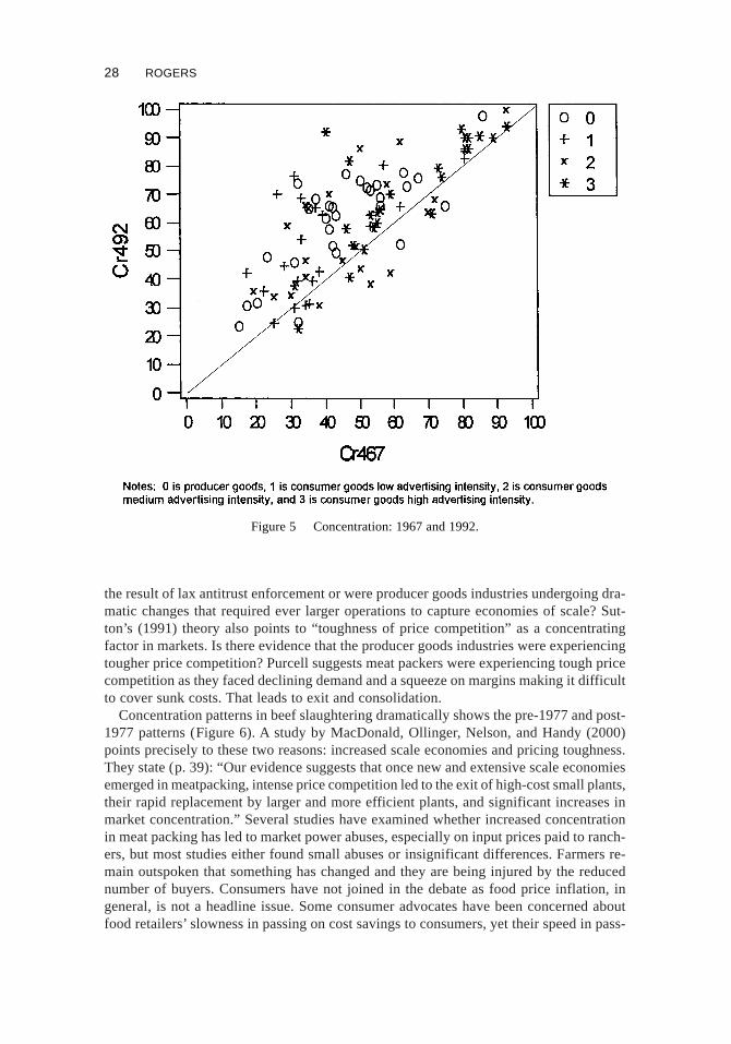
the result of lax antitrust enforcement or were producer goods industries undergoing dra-matic changes that required ever larger operations to capture economies of scale? Sut-ton’s (1991) theory also points to “toughness of price competition” as a concentratingfactor in markets. Is there evidence that the producer goods industries were experiencingtougher price competition? Purcell suggests meat packers were experiencing tough pricecompetition as they faced declining demand and a squeeze on margins making it difficultto cover sunk costs. That leads to exit and consolidation.

Concentration patterns in beef slaughtering dramatically shows the pre-1977 and post-1977 patterns (Figure 6). A study by MacDonald, Ollinger, Nelson, and Handy (2000)points precisely to these two reasons: increased scale economies and pricing toughness.They state (p. 39): “Our evidence suggests that once new and extensive scale economiesemerged in meatpacking, intense price competition led to the exit of high-cost small plants,their rapid replacement by larger and more efficient plants, and significant increases inmarket concentration.” Several studies have examined whether increased concentrationin meat packing has led to market power abuses, especially on input prices paid to ranch-ers, but most studies either found small abuses or insignificant differences. Farmers re-main outspoken that something has changed and they are being injured by the reducednumber of buyers. Consumers have not joined in the debate as food price inflation, ingeneral, is not a headline issue. Some consumer advocates have been concerned aboutfood retailers’ slowness in passing on cost savings to consumers, yet their speed in pass-

Figure 5 Concentration: 1967 and 1992.

28 ROGERS

ing on price increases. Again, studies on this issue have not supported any market powerabuses by retailers (see, e.g., Reed & Clark, 2000).

A similar pattern, but arriving a bit later, has occurred in hog slaughtering (Figure 7),where the consolidations have largely been in the 1990s. The U.S. Department of Agri-culture provides much more timely data on the industries for which it has oversight re-

Figure 6 Concentration in U.S. beef slaughtering, 1970–1999.

Figure 7 Concentration in U.S. hog slaughtering, 1970–1999.

STRUCTURAL CHANGE IN U.S. FOOD MANUFACTURING 29

sponsibilities than the Census Bureau provides. Some foresee the hog industry followingthe pattern of the broiler industry (e.g., Martinez, 1999), which has shown steady ad-vances in concentration (Figure 8) but without seller market power abuses. Each of thesemarkets is indicative of the new wave of increased concentration in markets without theuse of advertising.

4. SUMMARY

Aggregate concentration in the food and tobacco processing sector has an unbroken up-ward trend since at least 1954. The 20 largest food and tobacco firms are an impressiveand unique group among the more than 16,000 food firms. They controlled 44% of thesector’s value-added in 1992, up from 24% in 1967. These are massive firms with theaverage top 20 firms having 56 establishments, whereas even the firms among the secondlargest 100 firms had only an average of 7.3 establishments. Consolidations suggest thataggregate concentration will continue to increase as the food system enhances its bi-modal size distribution. Research by Rogers and Ma (1994) showed a positive relation-ship between aggregate concentration and market concentration. When the largest foodfirms (those among the top 100) enter a market, the outcome is not reduced market con-centration but increased concentration.

Market concentration has advanced in almost every food and tobacco processing mar-ket over time. The previous finding that the rising concentration was limited to the mostadvertising-intensive industries has been replaced with the finding that concentration isrising everywhere. If an industry was unconcentrated, it is likely to concentrate soon, if ithas not already done so in the 1990s. Milk and the other dairy industries are the nextindustries to show rising concentration, from what were once unconcentrated industries.

Figure 8 Concentration in U.S. broilers, 1954–1998.

30 ROGERS

We must now understand and monitor performance in a much more concentrated foodand tobacco sector and to do so with much less public information. Seller concentrationis high in many markets, but buyer concentration is dramatically higher given the specialcharacteristics of most agricultural markets. However, far less information is available onbuyer concentration than seller concentration, and the latter is not widely available andtimely as we still await concentration data for 1997. The Census needs to do a better jobby publishing more detailed concentration data and in a more timely fashion. With therise of industrialization and contract coordination, new measures need to be found to aidpolicy makers in assessing the performance of our more concentrated food system.

ACKNOWLEDGMENTS

This paper is based upon work supported by the Cooperative State Research, Extension,Education Service, U.S. Department of Agriculture, Massachusetts Agricultural Experi-ment Station, under Project No. Hatch 625/Multistate 165 (Manuscript number 3277)and the Food Marketing Policy Center, U. of Connecticut, Storrs, CT.

REFERENCES

Campbell, T.A. (1990). The millstone of debt: Exploring the cooperative past. American Cooper-ation, 5, 169–177.

Connor, J.M., & Geithman, F.E. (1988). Mergers in the food industries. Choices, Second Quarter.Connor, J.M., Rogers, R.T., & Bhagavan, V. (1996). Concentration change and countervailing power

in the U.S. food manufacturing industries. Review of Industrial Organization, 11, 473–492.Connor, J.M., Rogers, R.T., Marion, B.W., & Mueller, W.F. (1985). The food manufacturing indus-

tries. Massachusetts/Toronto: Lexington Books.Cotterill, R.W. (1997). The performance of agricultural marketing cooperatives in differentiated

product markets. Journal of Cooperation, 12, 23–34.Dimitri, C. (1999). Integration, coordination, and concentration in the fresh fruit and vegetable

industry. Fruit and Tree Nuts/FTS-285, Economic Research Service, U.S.D.A.Lanzillotti, R.F. (1960). The superior market power of food processing and agricultural supply firms—

Its relation to the farm problem. Journal of Farm Economics, XLII, 1228–1247.Lustgarten, S.H. (1975). The impact of buyer concentration in manufacturing industries. Review of

Economics and Statistics, 57(May), 125–132.MacDonald, J.M., Ollinger, M.E., Nelson, K.E., & Handy, C.H. (2000). Consolidation in U.S. meat-

packing. Agricultural Economic Report No. 785, Economic Research Service, U.S.D.A.Marion, B.W. (1986). The organization and performance of the U.S. food system. Lexington, MA:

D.C. Heath and Co.Marion, B.W., & Kim, D. (1991). Concentration change in selected food manufacturing industries:

The influence of mergers vs. internal growth. Agribusiness: An International Journal, 7, 415–431.Martinez, S.W. (1999). Vertical coordination in the pork and broiler industries: Implications for

pork and chicken products. Agricultural Economic Report No. 777, Economic Research Ser-vice, U.S.D.A.

Mueller, W.F., & Rogers, R.T. (1980). The role of advertising in changing concentration of indus-tries. Review of Economics and Statistics, 62(Feb.), 89–96.

Mueller, W.F., & Rogers, R.T. (1984). Changes in market concentration of manufacturing indus-tries, 1947–1977. Review of Industrial Organization, 1(1), 1–14.

Purcell, W.D. (1991, January). Antitrust policy in livestock: Which way in the 1990s? ResearchBulletin 1–91. Blacksburg, VA: Research Institute on Livestock Pricing, Agricultural Economics.

Reed, A.J., & Clark, J.S. (2000). Structural changes and competition in seven U.S. food markets.Technical Bulletin No. 1881. Economic Research Service, U.S.D.A.

Rogers, R.T. (2000). The U.S. food marketing system. In F.J. Francis (Ed.), Wiley encyclopedia offood science and technology (2nd ed.; pp. 2701–2724 ). New York: John Wiley & Sons.

STRUCTURAL CHANGE IN U.S. FOOD MANUFACTURING 31

Rogers, R.T., & Ma, Y.R. (1994, June). Concentration change in an era of lax antitrust enforcement:A comparison of two decades: 1967 to 1977 and 1977 to 1987, evidence from the food process-ing industries. Paper presented at the Northeast Regional Research Project NE-165 ResearchConference, Montreal, Quebec.

Rogers, R.T., & Petraglia, L.M. (1994). Agricultural cooperatives in food manufacturing: Implica-tions for market performance. Journal of Agricultural Cooperation, 9, 1–12.

Rogers, R.T., & Sexton, R.J. (1994). Assessing the importance of oligopsony power in agriculturalmarkets. American Journal of Agricultural Economics, 76, 1143–1150.

Rogers, R.T., & Tokle, R.J. 1999. The effects of television advertising on concentration: An update.New York Economic Review, XXX (Fall), 25–31.

Scherer, F.M., & Ross, D. (1990). Industrial market structure and economic performance (3rd ed.).Boston: Houghton Mifflin Company.

Sutton, J. (1991). Sunk costs and market structure. Cambridge, MA: MIT Press.United States Senate, 85th Congress, First Session. (1957). Concentration in American industry.

Report of the Subcommittee on Antitrust and Monopoly to the Committee of the Judiciary. Wash-ington, DC: United States Government Printing Office.

Zachary, G.P. (1999, March 8). Many industries are congealing into lineup of few dominant giants.Wall Street Journal, p. B1.

Richard T. Rogers is a professor of Resource Economics in the Department of Resource Econom-ics, University of Massachusetts, Amherst, and holds a Ph.D. in Agricultural Economics from theUniversity of Wisconsin–Madison. He is also a member of the Northeast Regional Research Project(NE-165) on Food Marketing issues titled “Private Strategies, Public Policies, and Food SystemPerformance.” His current research interests include the industrial economics of food manufac-turing markets and cooperatives.

32 ROGERS