String-Averaging Incremental Subgradients for … [email protected], [email protected],...
33
String-Averaging Incremental Subgradients for Constrained Convex Optimization with Applications to Reconstruction of Tomographic Images Rafael Massambone de Oliveira 1 , Elias Salomão Helou 1 and Eduardo Fontoura Costa 1 1 University of São Paulo - Institute of Mathematics and Computer Sciences, Department of Applied Mathematics and Statistics, São Carlos-SP, CEP 13566-590, Brazil E-mail: [email protected], [email protected], [email protected] Abstract. We present a method for non-smooth convex minimization which is based on subgradient directions and string-averaging techniques. In this approach, the set of available data is split into sequences (strings) and a given iterate is processed independently along each string, possibly in parallel, by an incremental subgradient method (ISM). The end-points of all strings are averaged to form the next iterate. The method is useful to solve sparse and large-scale non-smooth convex optimization problems, such as those arising in tomographic imaging. A convergence analysis is provided under realistic, standard conditions. Numerical tests are performed in a tomographic image reconstruction application, showing good performance for the convergence speed when measured as the decrease ratio of the objective function, in comparison to classical ISM. Keywords: convex optimization, incremental algorithms, subgradient methods, projection methods, string-averaging algorithms. arXiv:1610.05823v1 [math.OC] 18 Oct 2016
Transcript of String-Averaging Incremental Subgradients for … [email protected], [email protected],...
String-Averaging Incremental Subgradients forConstrained Convex Optimization with Applications toReconstruction of Tomographic Images
Rafael Massambone de Oliveira1, Elias Salomão Helou1 andEduardo Fontoura Costa1
1 University of São Paulo - Institute of Mathematics and Computer Sciences,Department of Applied Mathematics and Statistics, São Carlos-SP, CEP 13566-590,Brazil
E-mail: [email protected], [email protected],[email protected]
Abstract. We present a method for non-smooth convex minimization which is basedon subgradient directions and string-averaging techniques. In this approach, theset of available data is split into sequences (strings) and a given iterate is processedindependently along each string, possibly in parallel, by an incremental subgradientmethod (ISM). The end-points of all strings are averaged to form the next iterate. Themethod is useful to solve sparse and large-scale non-smooth convex optimizationproblems, such as those arising in tomographic imaging. A convergence analysis isprovided under realistic, standard conditions. Numerical tests are performed in atomographic image reconstruction application, showing good performance for theconvergence speed when measured as the decrease ratio of the objective function, incomparison to classical ISM.
Keywords: convex optimization, incremental algorithms, subgradient methods,projection methods, string-averaging algorithms.
arX
iv:1
610.
0582
3v1
[m
ath.
OC
] 1
8 O
ct 2
016
2
1. Introduction
A fruitful approach to solve an inverse problem is to recast it as an optimizationproblem, leading to a more flexible formulation that can be handled with differenttechniques. The reconstruction of tomographic images is a classical example of a problemthat has been explored by optimization methods, among which the well-knownincremental subgradient method (ISM) [40, 42, 49], that is a variation of the subgradientmethod [27, 44, 47], features nice performance in terms of convergence speed. Thereare many papers that discuss incremental gradient/subgradient algorithms forconvex/non-convex objective functions (smooth or not) with applications to severalfields [7, 9, 10, 40, 48–53]. Some examples of applications to tomographic imagereconstruction are found in [1, 12, 26, 34, 52]. In this paper, we consider a rathergeneral optimization problem that can be addressed by ISM and is useful fortomographic reconstruction and other problems, including to find solutions for ill-conditioned and/or large-scale linear systems. This problem consists of determining:
x ∈ arg min f (x)s.t. x ∈ X ⊂ Rn,
(1)
where:
(i) f (x) := P ∑mi=1 ξi fi(x) in which fi : Rn → R are convex (and possibly non-
differentiable) functions;
(ii) X is a non-empty, convex and closed set;
(iii) The set I = {S1, . . . , SP} is a partition of {1, . . . , m}, i.e., S` ∩ Sj = ∅ for any`, j ∈ {1, . . . , P} with ` 6= j and
⋃P`=1 S` = {1, . . . , m};
(iv) Given w` ∈ [0, 1] and S` ∈ I , ` = 1, . . . , P, the weights ξi satisfy ξi = w` for alli ∈ S`;
(v) ∑P`=1 w` = 1.
Problem (1) with conditions (i)-(v) is reduced to the classical problem ofminimizing ∑m
i=1 fi(x), s.t. x ∈ X, when w` = 1/P for all ` = 1, . . . , P. The reasonwhy we write the problem in this more complex way is twofold. On one hand, it iscommon to find problems in which a set of fixed weights are used to prioritize thecontribution of some component functions. For instance, in the context of distributednetworks, the component functions fi (also called “agents”) can be affected byexternal conditions, network topology, traffic, etc., making possible that some sets ofagents have a prevalent role on the network, which can be modeled by the weights(related to the corresponding subnets). On the other hand, the weights and thepartition, which bring flexibility to the model and could possibly be explored aimingfor instance at faster convergence, will fit naturally in our algorithmic framework.
We consider an approach that mixes ISM and string-averaging algorithms (SAalgorithms). The general form of the SA algorithm was proposed initially in [13]and applied in solving convex feasibility problems (CFPs) with algorithms that use
3
projection methods [13, 14, 43]. Strings are created so that ISM (more generally, anyε-incremental subgradient method) can be processed in an independent form foreach string (by step operators). Then, an average of string iterations is computed(combination operator), guiding the iterations towards the solution. To complete,approximate projections are used to maintain feasibility. We provide an analysis ofconvergence under reasonable assumptions, such as diminishing step-size rule andboundedness of the subgradients.
Some previous works in the literature have improved the understanding andpractical efficiency of ISM by creating more general algorithmic structures, enablinga broader analysis of convergence and making them more robust and accurate[35, 40, 42, 50, 51]. We improve on those results by adding a string-averagingstructure to the ISM that allows for an efficient parallel processing of a completeiteration which, consequently, can lead to fast convergence and suitable approximatesolutions. Furthermore, the presented techniques present better smoothing propertiesin practice, which is good for imaging tasks. These features are desirable, especiallywhen we seek to solve ill-conditioned/large scale problems. As mentioned at thebeginning of this section, one of our goals is to obtain an efficient method for solvingproblems of reconstruction of tomographic images from incompletely sampled data.
Although our work is closely linked to ISM, it is important to mention otherclasses of methods that can be applied to convex optimization problems. Underreasonable assumptions, problem (1) can be solved using proximal-type algorithms(for a description of some of the main methods, see [24]). For instance, in [23]the authors propose a proximal decomposition method derived from the Douglas-Rachford algorithm and establish its weak convergence in Hilbert spaces. Somevariants and generalizations of such methods can be found in [11, 17, 24, 25, 45].The bundle approach [32] is often used for numerically solving non-differentiableconvex optimization problems. Also, first order accelerated techniques [5, 6] form yetanother family of popular techniques for convex optimization problem endowedwith a certain separability property. The advantage of ISM over the aforementionedtechniques lies in its lightweight iterations from the computational viewpoint, noteven requiring sufficient decrease properties to be checked. Besides, ISM presentsa fast practical convergence rate in the first iterations which enables this techniqueto achieve good reconstructions within a small amount of time even for the hugeproblem sizes that appear, for example, in tomography.
The tomographic image reconstruction problem consists in finding an imagedescribed by a function ψ : R2 → R from samples of its Radon Transform, which canbe recast into solving the linear system
Rx = b, (2)
where R is the discretization of the Radon Transform operator, b contains the collectedsamples of the Radon Transform and the desired image is represented by the vectorx. We consider solving the problem (2), rewriting it as a minimization problem,
4
as in (1). Solving problem (2) from an optimization standpoint is not a new idea.In particular, [42] illustrates the application of some of the methods arising from ageneral framework to tomographic image reconstruction with a limited number ofviews. For the discretized problem (2), iterative methods such as ART (AlgebraicReconstruction Technique) [39], POCS (Projection Onto Convex Sets) [3, 22], andCimmino [21] have been widely used in the past.
Tomographic image reconstruction is an inverse problem in the sense that theimage ψ is to be obtained from the inversion of a linear compact operator, whichis well known to be an ill-conditioned problem. While the specific case of Radoninversion has an analytical solution, that was published in 1917 by Johann Radon (fordetails see [38]), both such analytical techniques and the aforementioned iterativemethods for linear systems of equations suffer from amplification of the statisticalnoise which, in practice, is always present in the right-hand side of (2). Therefore,methods designed to deal with noisy data have been developed, based on a maximumlikelihood approach, among which EM (Expectation Maximization) [46, 54], OS-EM(Ordered Subsets Expectation Maximization) [34], RAMLA (Row-Action MaximumLikelihood Algorithm) [12], BSREM (Block Sequential Regularized Expectation Maxi-mization) [26], DRAMA (Dynamic RAMLA) [41, 52], modified BSREM and relaxedOS-SPS (Ordered Subset-Separable Paraboloidal Surrogates) [1] are some of the bestknown in the literature. In [30], a variant of the EM algorithm was introduced, calledString-Averaging Expectation-Maximization (SAEM) algorithm. The SAEM algorithmwas used in problems of image reconstruction in Single-Photon Emission ComputerizedTomography (SPECT) and showed good performance in simulated and real datastudies. High-contrast images, with less noise and clearer object boundaries werereconstructed without incurring in more computation time. Besides the BSREM,DRAMA, modified BSREM and relaxed OS-SPS, that are relaxed algorithms for(penalized) maximum-likelihood image reconstruction in tomography, the methodintroduced in [28] considers an approach, based in OS-SPS, in which extra anatomicalboundary information is used. Other methods that use penalized models can befound in [20, 29]. Proximal methods were used in [2] to reconstruct images obtainedvia Cone Beam Computerized Tomography (CBCT) and Positron Emission Tomography(PET). In [20], the Majorize-Minimize Memory Gradient algorithm [18, 19] is studied andapplied to imaging tasks.
The paper is organized as follows: Section 2 contains some preliminary theoryinvolving incremental subgradient methods, optimality and feasibility operators andstring-averaging algorithm; Section 3 discusses the proposed algorithm to solve (1),(i)-(v); Section 4 shows theoretical convergence results; in Section 5 numerical testsare performed with reconstruction of tomographic images. Final considerations aregiven in Section 6.
5
2. Preliminary theory
Throughout the text, we will use the following notations: bold-type notations e.g. x,xi and xk
i are vectors whereas x is a number. We denote xi as the ith coordinate ofvector x. Moreover,
PX(x) := arg miny∈X‖y− x‖ , dX(x) := ‖x−PX(x)‖ ,
[x]+ := max {0, x} , f ∗ = infx∈X
f (x) and X∗ = {x ∈ X | f (x) = f ∗} ,
where we assume that X∗ 6= ∅.One of the main methods for solving (1) is the subgradient method, whose extensive
theory can be found in [8, 27, 32, 44, 47],
xk+1 = PX
(xk − λk
m
∑i=1
gki
), λk > 0, gk
i ∈ ∂ fi(xk), (3)
where the subdifferential of f : Rn → R at x (the set of all subgradients) can be definedby
∂ f (x) := {g | f (x) + 〈g, z− x〉 ≤ f (z), ∀z} . (4)
A similar approach to (3), known as incremental subgradient method, was studied firstlyby Kibardin in [37] and then analyzed by Solodov and Zavriev in [49], in which acomplete iteration of the algorithm can be described as follows:
xk0 = xk
xki = xk
i−1 − λkgki , i = 1, . . . , m, gk
i ∈ ∂ fi(xki−1) (5)
xk+1 = PX
(xk
m
).
A variant of this algorithm that uses projection onto X to compute the sub-iterationsxk
i was analyzed in [40].The method we propose in this paper for solving the problem given in (1), (i)-(v)
has the following general form described in [42]:
xk+1/2 = O f (λk, xk);xk+1 = VX(xk+1/2).
(6)
In the above equations, O f is called optimality operator and VX is the feasibilityoperator. This framework was created to handle quite general algorithms for convexoptimization problems. The basic idea consists in dividing an iterate in two parts: anoptimality step which tries to guide the iterate towards the minimizer of the objectivefunction (but not necessarily in a descent direction), followed by the feasibility stepthat drives the iterate in the direction of feasibility.
Next we enunciate a result due to Helou and De Pierro (see [42, Theorem 2.5]),establishing convergence of the method (6) under some conditions. This result is thekey for the convergence analysis of the algorithm we propose in section 3.
6
Theorem 2.1. The sequence {xk} generated by the method described in (6) converges in thesense that
dX∗(xk)→ 0 and limk→∞
f (xk) = f ∗,
if all of the following conditions hold:
Condition 1 (Properties of optimality operator). For every x ∈ X and for all sequenceλk ≥ 0, there exist α > 0 and a sequence ρk ≥ 0 such that the optimality operator O fsatisfies for all k ≥ 0
‖O f (λk, xk)− x‖2 ≤ ‖xk − x‖2 − αλk( f (xk)− f (x)) + λkρk. (7)
We further assume that the error term in the above inequality vanishes, i.e., ρk → 0 and weconsider a boundedness property for the optimality operator: there is γ > 0 such that
‖xk −O f (λk, xk)‖ ≤ λkγ. (8)
Condition 2 (Property of feasibility operator). For the feasibility operator VX, we imposethat for all δ > 0, exists εδ > 0 such that, if dX(xk+1/2) ≥ δ and x ∈ X we have
‖VX(xk+1/2)− x‖2 ≤ ‖xk+1/2 − x‖2 − εδ. (9)
Moreover, for all x ∈ X, VX(x) = x, i.e., x is a fixed point of VX.
Condition 3 (Diminishing step-size rule). The sequence {λk} satisfies
λk → 0+,∞
∑k=0
λk = ∞. (10)
Condition 4. The optimal set X∗ is bounded, {dX(xk)} is bounded and
[ f (PX(xk))− f (xk)]+ → 0.
Remark 2.2. Regarding the requirement [ f (PX(xk))− f (xk)]+ → 0, it holds if thereis a bounded sequence {vk} where vk ∈ ∂ f (PX(xk)) and dX(xk)→ 0. Indeed,
〈vk, y−PX(xk)〉 ≤ f (y)− f (PX(xk)), ∀ y ∈ Rn.
By Cauchy-Schwarz inequality, we have ‖vk‖‖PX(xk)− y‖ ≥ [ f (PX(xk))− f (y)]+.Taking y = xk, then dX(xk) → 0 ensures that [ f (PX(xk))− f (xk)]+ → 0. Therefore,under this mild boundedness assumption on the subdifferentials ∂ f (PX(xk)), provingthat dX(xk)→ 0 also ensures that [ f (PX(xk))− f (xk)]+ → 0.
Concerning the assumption dX(xk) → 0, Proposition 2.1 in [42] shows thatit holds if {dX(xk)} is bounded, λk → 0+, and Equation (8) plus Condition 2
hold. Since Condition 4 requires {dX(xk)} to be bounded, then we have that[ f (PX(xk))− f (xk)]+ → 0 just under the boundedness assumption on ∂ f (PX(xk)).Furthermore, Corollary 2.7 in [42] states that dX(xk)→ 0 if λk → 0+, Conditions 1 and2 hold and there is fl such that f (xk) ≥ fl for all k. Basically, the hypotheses of thiscorollary allow to show that {dX(xk)} is bounded and result follow by Proposition2.1. This is the situation that occurs in our numerical experiment. Such remarks areimportant to show how the hypotheses of our main convergence result (see Corollary4.5 in section 4) can be reasonable.
7
To state our algorithm in next section, we need to define the operators O f andVX. Below we present the last ingredient of our operator O f , the String-Averaging(SA) algorithm. Originally formulated in [13], SA algorithm consists of dividing anindex set I = {1, 2, . . . , η} into strings in the following manner
∆` :={
i`1, i`2, . . . , i`m(`)
}, (11)
where m(`) represents the number of elements in the string ∆` and ` ∈ {1, 2, . . . , N}.Let us consider X and Y as subsets of Rn where Y ⊆ X . The basic idea behindthe method consists in the sequential application of step operators F i`s : X → Y , foreach s = 1, 2, . . . , m(`) over each string ∆`, producing N vectors yk
` ∈ Y . Next, acombination operator F : YN → Y mixes, usually by weighted average, all vectors yk
`
to obtain yk+1. We refer to the index s as the step and the index k as the iteration.Therefore, given x0 ∈ X and strings ∆1, . . . , ∆N of I, a complete iteration of the SAalgorithm is computed, for each k ≥ 0, by equations
yk` := F i`m(`) ◦ . . . ◦ F i`2 ◦ F i`1
(xk)
, (12)
yk+1 := F ((yk1, . . . , yk
N)). (13)
The main advantage of this approach is to allow for computation of each vector yk` in
parallel at each iteration k, which is possible because the step operators F i`1 , . . . ,F i`m(`)
act along each string independently.
3. Proposed algorithm
Now we are ready to define O f and VX. Let us start by defining the optimalityoperator O f : R+ × Y→ Y, where Y is a non-empty, closed and convex set such that
X ⊂ Y ⊆ Rn. For this, let F i`s : R+ × Y → Y and F : YP → Y. Consider the set ofstrings ∆1 = S1, . . . , ∆P = SP and the weight set {w`}P
`=1 as defined in the problemgiven in (1) with conditions (iii)-(v). Then, given x ∈ Y and λ ∈ R+, we define
xi`0:= x, for all ` = 1, . . . , P, (14)
xi`s:= F i`s (λ, xi`s−1
) := xi`s−1− λgi`s
, s = 1, . . . , m(`), (15)
x` := xi`m(`), ` = 1, . . . , P, (16)
O f (λ, x) := F ((x1, . . . , xP)) :=P
∑`=1
w`x`, (17)
where gi`s∈ ∂ fi`s
(xi`s−1). Operators F i`s in (15) correspond to the step operators in
equation (12) of the SA algorithm and its definition is motivated by equation (5) of theincremental subgradient method. Function F in (17) corresponds to the combination
8
operator in (13) and performs a weighted average of the end-points x`, completingthe definition of the operator O f .
Now we need to define a feasibility operator VX. For that, we use the subgradientprojection [4, 22, 55, 56]. Let us start noticing that every convex set X 6= ∅ can bewritten as
X =t⋂
i=1
lev0(hi), (18)
where lev0(hi) := {x | hi(x) ≤ 0}. Each function hi : Rn → R (t is finite) is supposedto be convex. The feasibility operator VX : Rn → Rn is defined in [42] in the followingform:
VX := Sνtht◦ Sνt−1
ht−1◦ . . . ◦ Sν1
h1. (19)
This definition assumes that there is σ ∈ (0, 1] such that νi ∈ [σ, 2− σ] for all i. Eachoperator Sν
h : Rn → Rn in the previous definition is constructed using a ν-relaxedversion of the subgradient projection with Polyak-type step-sizes , i.e.,
Sνh (x) :=
{x− ν
[h(x)]+‖h‖2 h, if h 6= 0;
x, otherwise,(20)
where ν ∈ (0, 2) and h ∈ ∂h(x).In order to get a better understanding of the behavior of our feasibility
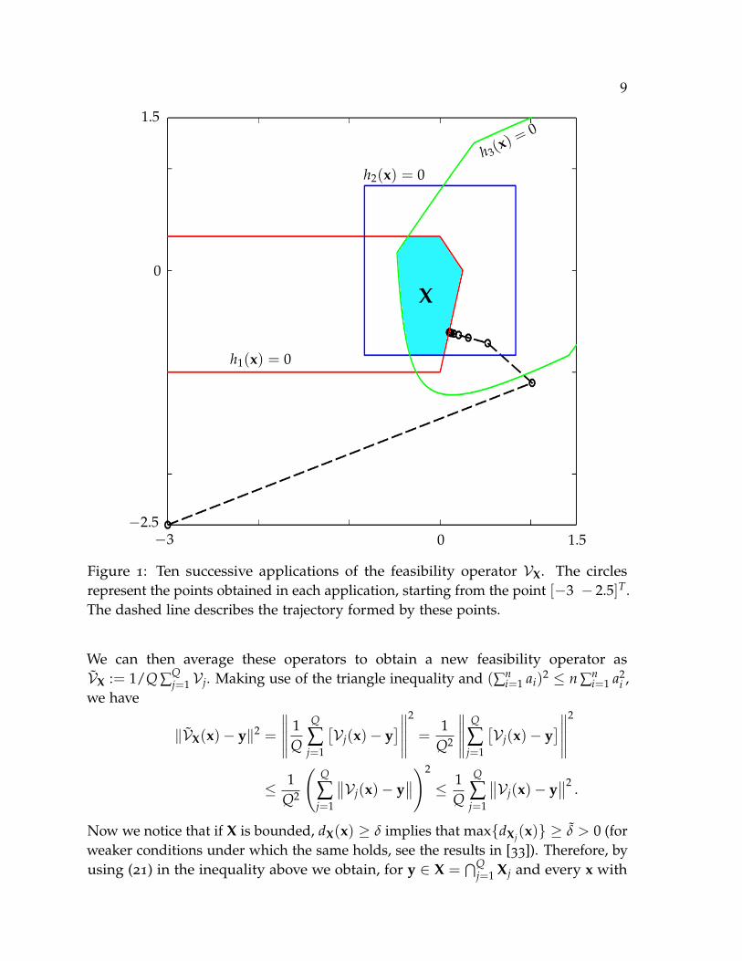
operator, Figure 1 shows the trajectory taken by successive applications of theoperator VX. The feasible set X is the intersection of the zero sublevel sets of thefollowing convex functions: h1(x) = 〈a, x〉 + 2‖x‖1 − 1, h2(x) = 3‖x‖∞ − 2.5 andh3(x) = ‖Ax− a‖1 + 2‖Bx− c‖2 − 10 where
A =
[2 1−1 3
], B =
[1 0−2 2
], a = [2 1]T and c = [1 − 2]T.
To obtain VX(x) = Sν3h3◦ Sν2
h2◦ Sν1
h1(x), we compute the subgradients hi ∈ ∂hi(si−1),
i = 1, . . . , 3, such that s0 := x and si := Sνihi(si−1). We choose [−3 − 2.5]T as an initial
point and the following relaxation parameters: ν1 = 0.5, ν2 = 0.6 and ν3 = 0.7.
Remark 3.1. A string-averaging version of the feasibility operator can easily bederived in the following manner. Consider Q strings Vj := {ij
1, ij2, . . . , ij
κ(j)} ⊂{1, . . . , t} such that
⋃Qj=1 Vj = {1, . . . , t}, where κ(j) is the number of elements
in the string Vj. Then, for each j = 1, . . . , Q, we define the string feasibility operator Vjas
Vj := Sν
ijκ(j)
hijκ(j)
◦ Sν
ijκ(j)−1
hijκ(j)−1
◦ . . . ◦ Sν
ij1h
ij1
,
each satisfying for y ∈ Xj :=⋂
i∈Vjlev0(hi) and every x with dXj(x) ≥ δ:
‖Vj(x)− y‖2 ≤ ‖x− y‖2 − εjδ. (21)
9
h1(x) = 0
h2(x) = 0h3(x
) =0
X
1.50−3
1.5
0
−2.5
Figure 1: Ten successive applications of the feasibility operator VX. The circlesrepresent the points obtained in each application, starting from the point [−3 − 2.5]T.The dashed line describes the trajectory formed by these points.
We can then average these operators to obtain a new feasibility operator asVX := 1/Q ∑Q
j=1 Vj. Making use of the triangle inequality and (∑ni=1 ai)
2 ≤ n ∑ni=1 a2
i ,we have
‖VX(x)− y‖2 =
∥∥∥∥∥1Q
Q
∑j=1
[Vj(x)− y
]∥∥∥∥∥
2
=1
Q2
∥∥∥∥∥Q
∑j=1
[Vj(x)− y
]∥∥∥∥∥
2
≤ 1Q2
(Q
∑j=1
∥∥Vj(x)− y∥∥)2
≤ 1Q
Q
∑j=1
∥∥Vj(x)− y∥∥2 .
Now we notice that if X is bounded, dX(x) ≥ δ implies that max{dXj(x)} ≥ δ > 0 (forweaker conditions under which the same holds, see the results in [33]). Therefore, byusing (21) in the inequality above we obtain, for y ∈ X =
⋂Qj=1 Xj and every x with
10
dX(x) ≥ δ:
‖VX(x)− y‖2 ≤ 1Q
Q
∑j=1
{‖x− y‖2 − ε
jδj
},
where δj := dXj(x). Therefore:
‖VX(x)− y‖2 ≤ ‖x− y‖2 − εδ,
where εδ = minj∈{1,...,Q}{εjδ}.
The above argument suggests that if the operators Vj satisfy Condition 2 withX replaced by Xj, then its average also will satisfy Condition 2 with X replaced by⋂Q
j=1 Xj. To the best of our knowledge, the previous discussion presents a first step togeneralize some of the results from [13, 15, 16] towards averaging strings of inexactprojections, or more specifically, averaging of Fejér-monotone operators. We do notmake use of averaged feasibility operators in this paper for clarity of presentation andalso because our numerical examples can be handled in the classical way, withoutstring averaging, since our model has few constraints.
With the optimality and feasibility operators already defined, we present acomplete description of the algorithm we propose to solve the problem defined in(1), (i)-(v).
Algorithm 3.2 (String-averaging incremental subgradient method).
Input: Choose an initial vector x0 ∈ Y and a sequence of step-sizes λk ≥ 0.
Iteration: Given the current iteration xk, do
Step 1. (Step operators) Compute independently for each ` = 1, . . . , P:
xki`0= xk,
xki`s= F i`s (λk, xk
i`s−1), s = 1, . . . , m(l),
xk` = xk
i`m(`), (22)
where i`s ∈ ∆` := S` for each s = 1, . . . , m(`) and F i`s is defined in (15).Step 2. (Combination operator) Use the end-points xk
` obtained in Step 1 and theoptimality operator O f defined in (17) to obtain:
xk+1/2 = O f (λk, xk). (23)
Step 3. Apply feasibility operator VX defined in (19) on the sub-iteration xk+1/2 toobtain:
xk+1 = VX(xk+1/2). (24)
Step 4. Update k and return to Step 1.
11
4. Convergence analysis
Along this section, we denote FS`(x) = ∑m(`)s=1 fi`s
(x) for each ` = 1, . . . , P. Thefollowing subgradient boundedness assumption is key in this paper: for all ` and s,
Ci`s= sup
k≥0
{‖g‖ | g ∈ ∂ fi`s
(xk) ∪ ∂ fi`s(xk
i`s−1)
}< ∞. (25)
Recall that Theorem 2.1 is the main tool for the convergence analysis, so we will showthat each of its conditions are valid under assumption (25). We present auxiliaryresults in the next two lemmas.
Lemma 4.1. Let {xk} be the sequence generated by Algorithm 3.2 and suppose thatsubgradient boundedness assumption (25) holds. Then, for each ` and s and for all k ≥ 0, wehave
(i) fi`s(xk)− fi`s
(xki`s−1
) ≤ Ci`s‖xk
i`s−1− xk‖. (26)
(ii) ‖xki`s− xk‖ ≤ λk
s
∑r=1
Ci`r. (27)
(iii) For all y ∈ Rn, we have⟨
m(`)
∑s=1
gki`s
, y− xk
⟩≤ FS`(y)− FS`(x
k) + 2λk
m(`)
∑s=2
Ci`s
(s−1
∑r=1
Ci`r
), (28)
where gki`s∈ ∂ fi`s
(xki`s−1
).
Proof. (i) By definition of the subdifferential ∂ fi`s(xk), we have
fi`s(xk)− fi`s
(xki`s−1
) ≤ −〈vki`s
, xki`s−1− xk〉,
where vki`s∈ ∂ fi`s
(xk). The result follows from the Cauchy-Schwarz inequalityand the subgradient boundedness assumption (25).
(ii) Developing the equation xki`s= xk
i`s−1− λkgk
i`sfor each s = 1, . . . , m(`) yields,
‖xki`1− xk‖ = ‖xk − λkgk
i`1− xk‖ ≤ λkCi`1
,
‖xki`2− xk‖ ≤ ‖xk
i`1− xk‖+ λk‖gk
i`2‖ ≤ λk(Ci`1
+ Ci`2),
......
...
‖xki`s− xk‖ ≤ ‖xk
i`s−1− xk‖+ λk‖gk
i`s‖ ≤ λk
s
∑r=1
Ci`r.
(iii) By Cauchy-Schwarz inequality and definition of the subdifferential ∂ fi`s(xk
i`s−1)
12
we have,⟨
m(`)
∑s=1
gki`s
, y− xk
⟩=
m(`)
∑s=1〈gk
i`s, xk
i`s−1− xk〉+
m(`)
∑s=1〈gk
i`s, y− xk
i`s−1〉
≤m(`)
∑s=1‖gk
i`s‖‖xk − xk
i`s−1‖+
m(`)
∑s=1
( fi`s(y)− fi`s
(xki`s−1
))
=m(`)
∑s=2‖gk
i`s‖‖xk − xk
i`s−1‖+ FS`(y)− FS`(x
k)
−m(`)
∑s=2
( fi`s(xk
i`s−1)− fi`s
(xk)).
By eqs. (26), (27) and the subgradient boundedness assumption (25) we obtain,⟨
m(`)
∑s=1
gki`s
, y− xk
⟩≤
m(`)
∑s=2‖gk
i`s‖‖xk − xk
i`s−1‖+ FS`(y)− FS`(x
k)
+m(`)
∑s=2‖vk
i`s‖‖xk − xk
i`s−1‖
≤ FS`(y)− FS`(xk) +
m(`)
∑s=2
(‖gki`s‖+ ‖vk
i`s‖)(
λk
s−1
∑r=1
Ci`r
)
≤ FS`(y)− FS`(xk) + 2λk
m(`)
∑s=2
Ci`s
(s−1
∑r=1
Ci`r
).
The following Lemma is useful to analyze the convergence of the Algorithm 3.2.
Lemma 4.2. Let {xk} be the sequence generated by Algorithm 3.2 and suppose thatassumption (25) holds. Then, there is a positive constant C such that, for all y ∈ Y ⊃ X andfor all k ≥ 0 we have
‖O f (λk, xk)− y‖2 ≤ ‖xk − y‖2 − 2P
λk( f (xk)− f (y)) + Cλ2k, (29)
Proof. Initially, we can develop equation (22) for each ` = 1, . . . , P and obtain
xk` = xk − λk
m(`)
∑s=1
gki`s
, where gki`s∈ ∂ fi`s
(xki`s−1
). Thus, from equation (23) we have
for all k ≥ 0,
O f (λk, xk) =P
∑`=1
w`xk`
=P
∑`=1
w`
(xk − λk
m(`)
∑s=1
gki`s
)
= xk − λk
P
∑`=1
w`
m(`)
∑s=1
gki`s
.
13
Using the above equation we obtain for all y ∈ Y and for all k ≥ 0,
‖O f (λk, xk)− y‖2 =
∥∥∥∥∥xk − y− λk
P
∑`=1
w`
m(`)
∑s=1
gki`s
∥∥∥∥∥
2
= ‖xk − y‖2 − 2
⟨xk − y, λk
P
∑`=1
w`
m(`)
∑s=1
gki`s
⟩+
∥∥∥∥∥λk
P
∑`=1
w`
m(`)
∑s=1
gki`s
∥∥∥∥∥
2
= ‖xk − y‖2 + 2λk
P
∑`=1
w`
⟨m(`)
∑s=1
gki`s
, y− xk
⟩+ λ2
k
∥∥∥∥∥P
∑`=1
w`
m(`)
∑s=1
gki`s
∥∥∥∥∥
2
.
Now, using Lemma 4.1 (iii), triangle inequality and P ∑P`=1 w`FS`(x) = f (x) we have,
‖O f (λk, xk)− y‖2 ≤ ‖xk − y‖2 − 2λk
P
∑`=1
w`
[FS`(x
k)− FS`(y)− 2λk
m(`)
∑s=2
Ci`s
(s−1
∑r=1
Ci`r
)]
+λ2k
∥∥∥∥∥P
∑`=1
w`
m(`)
∑s=1
gki`s
∥∥∥∥∥
2
≤ ‖xk − y‖2 − 2λk
(P
∑`=1
w`FS`(xk)−
P
∑`=1
w`FS`(y)
)
+4λ2k
P
∑`=1
w`
[m(`)
∑s=2
Ci`s
(s−1
∑r=1
Ci`r
)]+ λ2
k
(P
∑`=1
w`
m(`)
∑s=1‖gk
i`s‖)2
= ‖xk − y‖2 − 2λkP( f (xk)− f (y)) + 4λ2
k
P
∑`=1
w`
[m(`)
∑s=2
Ci`s
(s−1
∑r=1
Ci`r
)]
+λ2k
(P
∑`=1
w`
m(`)
∑s=1‖gk
i`s‖)2
.
Finally, by subgradient boundedness assumption (25), we obtain for all y ∈ Y andfor all k ≥ 0,
‖O f (λk, xk)− y‖2 ≤ ‖xk − y‖2 − 2λkP( f (xk)− f (y))
+λ2k
4
P
∑`=1
w`
[m(`)
∑s=2
Ci`s
(s−1
∑r=1
Ci`r
)]+
(P
∑`=1
w`
m(`)
∑s=1
Ci`s
)2
= ‖xk − y‖2 − 2P
λk( f (xk)− f (y)) + Cλ2k.
The next two propositions aim at showing that, under some mild additionalhypothesis, O f and VX satisfy Conditions 1-2.
Proposition 4.3. Let {xk} be the sequence generated by Algorithm 3.2 and suppose thatsubgradient boundedness assumption (25) holds. Then, if λk → 0+, the optimality operatorO f satisfies Condition 1 of Theorem 2.1.
14
Proof. Lemma 4.2 ensures that for all x ∈ X ⊂ Y we have,
‖O f (λk, xk)− x‖2 ≤ ‖xk − x‖2 − 2P
λk( f (xk)− f (x)) + Cλ2k.
Defining α = 2/P and ρk = λkC ≥ 0, equation (7) is satisfied and ρk → 0.Furthermore, by triangle inequality and subgradient boundedness assumption (25)we have,
‖O f (λk, xk)− xk‖ =∥∥∥∥∥
P
∑`=1
w`xk` − xk
∥∥∥∥∥
=
∥∥∥∥∥xk − λk
P
∑`=1
w`
m(`)
∑s=1
gki`s− xk
∥∥∥∥∥
= λk
∥∥∥∥∥P
∑`=1
w`
m(`)
∑s=1
gki`s
∥∥∥∥∥
≤ λk
P
∑`=1
w`
m(`)
∑s=1
Ci`s,
implying that equation (8) is satisfied with γ = ∑P`=1 w` ∑
m(`)s=1 Ci`s
. Therefore,Condition 1 is satisfied.
Proposition 4.4. ([42], Proposition 3.4) Let xk+1/2 given in (23) be the first element sk0
of the sequence {ski }, i = 1, . . . , t, given as sk
i := Sνihi(sk
i−1). In this sense, consider thathk
i ∈ ∂hi(ski−1). Suppose that for some index j, the set lev0(hj) is bounded. In addition,
consider that all sequences{
hki}
are bounded. Then, VX satisfies Condition 2 of Theorem 2.1.
The main result of the paper is given next.
Corollary 4.5. Let {xk} be the sequence generated by Algorithm 3.2 and suppose thatsubgradient boundedness assumption (25) holds. In addition, suppose that lev0(hj) isbounded for some j and all sequences {hk
i } are bounded. Then, if Conditions 3-4 of Theorem2.1 hold, we have
dX∗(xk)→ 0 and limk→∞
f (xk) = f ∗.
Proof. Propositions 4.3 and 4.4 state that operators O f and VX satisfy Conditions 1-2.Therefore, the result is obtained applying Theorem 2.1.
Recall that we discuss the reasonability of the Condition 4 as a hypothesis forthis corollary in Remark 2.2.
15
5. Numerical experiments
In this section, we apply the problem formulation (1), (i)-(v) and the method givenin Algorithm 3.2 to the reconstruction of tomographic images from few views, andwe explore results obtained from simulated and real data to show that the methodis competitive when compared with the classic incremental subgradient algorithm.Let us start with a brief description of the problem. The task of reconstructingtomographic images is related to the mathematical problem of finding a functionψ : R2 → R from its line integrals along straight lines. More specifically, we desire tofind ψ given the following function:
R[ψ](θ, t) :=∫
Rψ(t(cos θ, sin θ)T + s(− sin θ, cos θ)T) ds. (30)
The application ψ 7→ R[ψ] is so-called Radon Transform and for a fixed θ, Rθ[ψ](t)is known as a projection of ψ. For a detailed discussion about the physical andmathematical aspects involving tomography and the definition in (30), see, forexample [31, 38, 39].
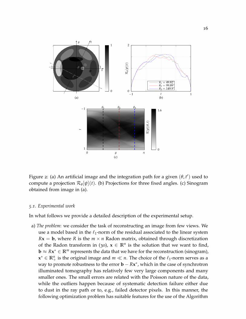
We now provide an example to better understand the geometric meaning of thedefinition of Radon transform. We can display ψ as a picture if we assign to eachvalue in [0, 1], a grayscale such as in Figure 2-(a). Here we use an artificial imagemade up of a sum of indicator functions of ellipses. The bar on the right indicates thegrayscale used. We also show the axes t, x, y and the integration path for a given pair(θ, t′), which appears as the dashed line segment. The t-axis directions vary accordingto the number of angles adopted for the reconstruction process. In general, θ ∈ [0, π)
because R[ψ](θ + π,−t) = R[ψ](θ, t). For a fixed angle θ, the projection Rθ[ψ](t) iscomputed for each t′ ∈ [−1, 1]. Figure 2-(b) shows the projections obtained for threefixed angles θ: θ1, θ2 and θ3. Its representation given in Figure 2-(c) as an image inthe θ × t coordinate system is called sinogram. We also call the Radon transform at afixed angle a view or projection.
The Radon transform models the data in a tomographic image reconstructionproblem. That is, for reconstruction of the function ψ, we must go from Figure 2-(c)to the desired image in Figure 2-(a), i.e., it would be desirable to calculate the inverseR−1. However, as already mentioned, the Radon Transform is a compact operatorand therefore its inversion is an ill-conditioned problem. In fact, for n = 2 and n = 3,Radon obtained inversion formulas involving first and second order differentiationof the data [39], respectively, implying in an unstable process due the increase ofthe error propagation in presence of perturbed data (when noise is present, whichmay occur due to width of the x-ray beam, scatter, hardening of the beam, photonstatistics, detector inaccuracies, etc [31]). Other difficulties arise when using analyticalsolutions in practice due to, for example, the limited number of views that oftenoccurs. This is why more sophisticated optimization models are useful, and it isdesirable to use an objective function and constraints that forces the consistency ofthe solution to the data and guarantees stability of the solution.
16
0
1
0
2
−1 1
Rθ[ψ](
t)
t
−1
10 π
t
θ0
1.6
R[ψ](
θ,t)
6
-
�������������������
q
q
HHHH
HHHH
HHHH
HHHH
HHHH
HHHH
HHHHY
HHj
qt′
x
y t
(a) (b)
(c)
�θ−1 1
θ1 θ2 θ3
θ1 = 49.82◦θ2 = 99.89◦θ3 = 149.9◦
Figure 2: (a) An artificial image and the integration path for a given (θ, t′) used tocompute a projection Rθ[ψ](t). (b) Projections for three fixed angles. (c) Sinogramobtained from image in (a).
5.1. Experimental work
In what follows we provide a detailed description of the experimental setup.
a) The problem: we consider the task of reconstructing an image from few views. Weuse a model based in the `1-norm of the residual associated to the linear systemRx = b, where R is the m× n Radon matrix, obtained through discretizationof the Radon transform in (30), x ∈ Rn is the solution that we want to find,b ≈ Rx∗ ∈ Rm represents the data that we have for the reconstruction (sinogram),x∗ ∈ Rn
+ is the original image and m� n. The choice of the `1-norm serves as away to promote robustness to the error b− Rx∗, which in the case of synchrotronilluminated tomography has relatively few very large components and manysmaller ones. The small errors are related with the Poisson nature of the data,while the outliers happen because of systematic detection failure either dueto dust in the ray path or to, e.g., failed detector pixels. In this manner, thefollowing optimization problem has suitable features for the use of the Algorithm
17
3.2:
min f (x) = ‖Rx− b‖1s.t. h(x) = TV(x)− τ ≤ 0,
x ∈ Rn+.
(31)
Note that the objective function f (x) = ∑mi=1 |〈ri, x〉 − bi| = ∑m
i=1 fi(x), where rirepresents the i-th row of R. In comparison to (1) (i)-(v), model (31) suggestsconstant weights w` = 1/P for all ` = 1, . . . , P to satisfy conditions (iv) and (v).In our tests, we use P = 1, . . . , 6 and, to build the sets S`, we ordered the indicesof the data randomly and then distributed in P equally sized sets (or as closeto it as possible) aiming at satisfying condition (iii). We also assume that theimage x∗ to be reconstructed has large approximately constant areas, as is oftenthe case in tomographic images. Operator TV : Rn → R+ is called total variationand is defined by
TV(x) =r2
∑i=1
r1
∑j=1
√(xi,j − xi−1,j
)2+(xi,j − xi,j−1
)2,
where x = [xq]T, q ∈ {1, . . . , n}, n = r1r2 and xi,j := x(i−1)r1+j. We have alsoused the boundary conditions x0,j = xi,0 = 0 and τ = TV(x∗).
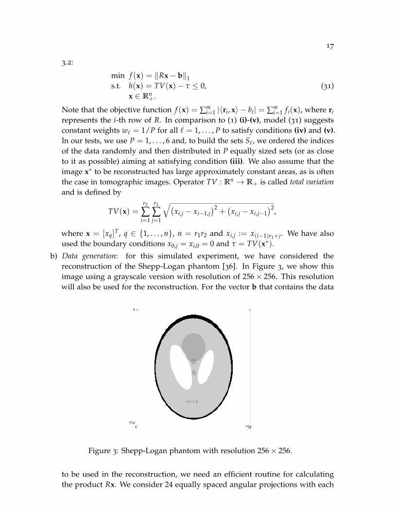
b) Data generation: for this simulated experiment, we have considered thereconstruction of the Shepp-Logan phantom [36]. In Figure 3, we show thisimage using a grayscale version with resolution of 256× 256. This resolutionwill also be used for the reconstruction. For the vector b that contains the data
Figure 3: Shepp-Logan phantom with resolution 256× 256.
to be used in the reconstruction, we need an efficient routine for calculatingthe product Rx. We consider 24 equally spaced angular projections with each
18
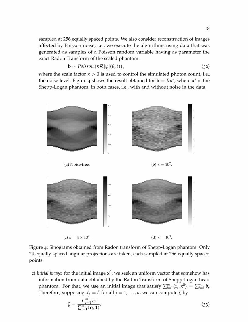
sampled at 256 equally spaced points. We also consider reconstruction of imagesaffected by Poisson noise, i.e., we execute the algorithms using data that wasgenerated as samples of a Poisson random variable having as parameter theexact Radon Transform of the scaled phantom:
b ∼ Poisson (κR[ψ](θ, t)) , (32)
where the scale factor κ > 0 is used to control the simulated photon count, i.e.,the noise level. Figure 4 shows the result obtained for b = Rx∗, where x∗ is theShepp-Logan phantom, in both cases, i.e., with and without noise in the data.
(a) Noise-free. (b) κ = 102.
(c) κ = 4× 10². (d) κ = 103.
Figure 4: Sinograms obtained from Radon transform of Shepp-Logan phantom. Only24 equally spaced angular projections are taken, each sampled at 256 equally spacedpoints.
c) Initial image: for the initial image x0, we seek an uniform vector that somehow hasinformation from data obtained by the Radon Transform of Shepp-Logan headphantom. For that, we use an initial image that satisfy ∑m
i=1〈ri, x0〉 = ∑mi=1 bi.
Therefore, supposing x0j = ζ for all j = 1, . . . , n, we can compute ζ by
ζ =∑m
i=1 bi
∑mi=1〈ri, 1〉 , (33)
19
where 1 is the n-vector whose components are all equal to 1.
d) Applying Algorithm 3.2: step-size sequence {λk} was determined by the formula
λk = (1− ρck)λ0
αks/P + 1, (34)
where the sequence ck starts with c0 = 0 and the following terms are given by
ck =
⟨xk−1/2 − xk−1, xk − xk−1/2⟩
∥∥xk−1/2 − xk−1∥∥ ∥∥xk − xk−1/2
∥∥ .
Each ck is the cosine of the angle between the directions taken by optimalityand feasibility operators in the previous iteration. Thus, the factor (1− ρck)
serves as an empirical way to prevent oscillations. Finally, we use λ0 =
µ∥∥Rx0 − b
∥∥1 /∥∥g0∥∥2, where µ is the number of parcels in which the sum is
divided and g0 is a subgradient of objective function in x0. Other free parametersin (34) were tuned and set to: ρ = 0.999, s = 0.51 and α = 1.0.
Now we need to calculate the subgradients for the objective function andTV. Since the vector
sign(x) = [ui]T, such that ui :=
1, if xi > 0,0, if xi = 0,−1, otherwise
belongs to the set ∂ ‖x‖1, then the theorem 4.2.1, p. 263 in [32] guarantees that
RTsign(Rx− b) ∈ ∂ ‖Rx− b‖1 ,
and this subgradient will be used in our experiments. In particular, for eachk ≥ 0, ` = 1, . . . , P and s = 1, . . . , m(`) we use
gki`s=
ri`s, if 〈ri`s
, xki`s−1〉 − bi`s
> 0,
−ri`s, if 〈ri`s
, xki`s−1〉 − bi`s
< 0,
0, otherwise.
(35)
A subgradient h = [ti,j] for h(x) = TV(x)− τ can be computed by
ti,j =2xi,j − xi,j−1 − xi−1,j√
(xi,j − xi,j−1)2 + (xi,j − xi−,j)2
+xi,j − xi,j+1√
(xi,j+1 − xi,j)2 + (xi,j+1 − xi−1,j+1)2
+xi,j − xi+1,j√
(xi+1,j − xi,j)2 + (xi+1,j − xi+1,j−1)2,
(36)
where, if any denominator is zero, we annul the correspondent parcel.
Once we have determined the strings by setting ∆1 = S1, . . . , ∆P = SP andweights (w` = 1/P for all `), the step-size sequence λk in (34), initial image x0 in(33) and subgradients gk
i`s∈ ∂ fi`s
(xki`s−1
) in (35), optimality operator O f (14)-(17) can be
20
applied. By considering the subdifferential of ‖x‖1, it is clear that ∂ f (x) is uniformlybounded, ensuring that assumption (25) holds. Moreover, since ρ ∈ [0, 1), α > 0,s ∈ (0, 1] and ck ∈ [−1, 1], by Cauchy-Schwarz inequality we can ensure that λk > 0and that Condition 3 of Theorem 2.1 holds.
Using h ∈ ∂h(x) defined in (36), operator Sνh can be computed by equation
(20), such that, in our tests, we use ν = 1. The feasibility operator is thus given byVX = PRn
+◦ Sν
h (see equation (19)). The projection step can be regarded as a specialcase of the operator Sν
g with ν = 1 and g = dRn+
. It is easy to see that VX defined inthis way satisfies the conditions established in the Proposition 4.4.
In conclusion, once ‖Rx− b‖1 ≥ 0, Corollary 2.7 in [42] implies that{
dX(xk)}→
0 (the sequence is bounded). Since ∂ f (x) is uniformly bounded, we have that[f (PX(xk))− f (xk)
]+ → 0 and Condition 4 of Theorem 2.1 holds. Thus, Corollary
4.5 can be applied ensuring convergence of the Algorithm 3.2.
5.2. Image reconstruction analysis
To run the experiments, we used a computer with processor Intel Core i7-4790 CPU@ 3.60 GHz x8 and 16 GB of memory. The operating system used was Linux and theimplementation was realized in C++. Figure 5 shows the decrease of the objectivefunction with respect to computation time to compare convergence speed and imagequality in the performed reconstructions. Furthermore, in order to obtain a moremeaningful analysis, we consider the graphic of the total variation TV(x) and therelative squared error,
RSE(x) =‖x− x∗‖2
‖x∗‖2 .
Note that the RSE metric requires information on the desired image. Also we showgraphs of TV(xk) as function of f (xk).
When we use P = 2, . . . , 6 (algorithm is executed with 2-6 strings), it is possibleto observe a faster decrease in the values of the objective function f (xk) as the runningtime increases, if compared to the case where P = 1. Since there is no guaranteethat algorithm produces a descent direction in each iteration, it is important to notethat, in some of the tests, the intensity of the oscillation, i.e., f (xk+1) − f (xk) forf (xk+1) > f (xk), decreases as the number of strings increases (note, for example, thealgorithm performance with 5 and 6 strings, from 0 to about 40 seconds). A similarbehavior can be noted for values TV(xk). For 4-6 strings, the algorithm is able toprovide images with a more appropriate TV level, approaching the feasible regionmore quickly. Even if closer to satisfying the constraints, for methods with a largernumber of strings, the values of RSE(xk) and of the objective function decrease withlower intensity oscillations and reach lower values within the same computation time.Interestingly, the experiments with noisy data show that the algorithm generates asharp decrease in the intensity of oscillation precisely where image quality seems toreach a good level. The study of conditions under which we can establish a stopping
21
10−1
100
101
102
103
104
10−2 10−1 100 101 102 103
∥ ∥ Rxk−b∥ ∥ 1
Time (seconds)
10−5
10−4
10−3
10−2
10−1
100
101
102
10−2 10−1 100 101 102 103
RSE(x
k)
Time (seconds)
103
104
105
10−2 10−1 100 101 102 103
TV(x
k)
Time (seconds)
103
104
10−1 100 101 102 103
TV(x
k)
∥∥Rxk − b∥∥1
ISM2 strings3 strings4 strings5 strings6 strings
ISM2 strings3 strings4 strings5 strings6 strings
ISM2 strings3 strings4 strings5 strings6 strings
ISM2 strings3 strings4 strings5 strings6 strings
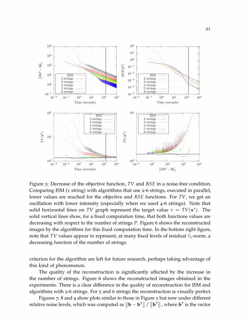
Figure 5: Decrease of the objective function, TV and RSE in a noise-free condition.Comparing ISM (1 string) with algorithms that use 2-6 strings, executed in parallel,lower values are reached for the objective and RSE functions. For TV, we get anoscillation with lower intensity (especially when we used 4-6 strings). Note thatsolid horizontal lines on TV graph represent the target value τ = TV(x∗). Thesolid vertical lines show, for a fixed computation time, that both functions values aredecreasing with respect to the number of strings P. Figure 6 shows the reconstructedimages by the algorithms for this fixed computation time. In the bottom right figure,note that TV values appear to represent, at many fixed levels of residual `1-norm, adecreasing function of the number of strings.
criterion for the algorithm are left for future research, perhaps taking advantage ofthis kind of phenomenon.
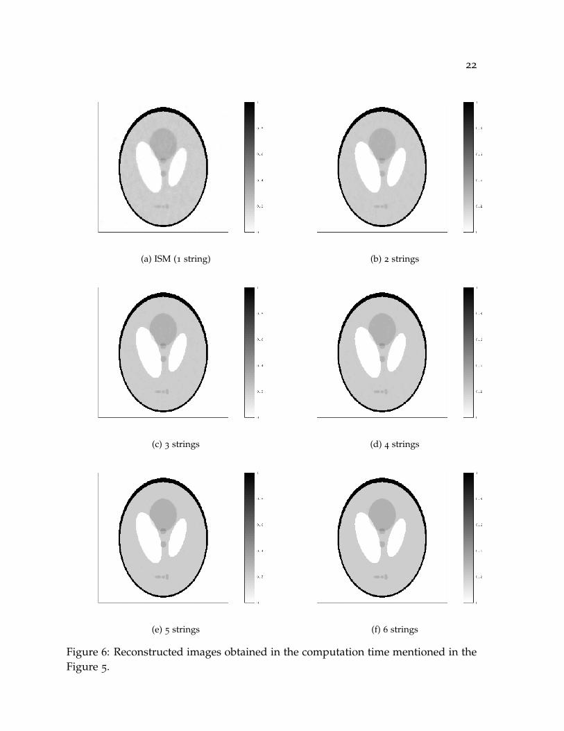
The quality of the reconstruction is significantly affected by the increase inthe number of strings. Figure 6 shows the reconstructed images obtained in theexperiments. There is a clear difference in the quality of reconstruction for ISM andalgorithms with 2-6 strings. For 5 and 6 strings the reconstruction is visually perfect.
Figures 7, 8 and 9 show plots similar to those in Figure 5 but now under differentrelative noise levels, which was computed as
∥∥b− b†∥∥ /∥∥b†
∥∥ , where b† is the vector
22
(a) ISM (1 string) (b) 2 strings
(c) 3 strings (d) 4 strings
(e) 5 strings (f) 6 strings
Figure 6: Reconstructed images obtained in the computation time mentioned in theFigure 5.
23
that contains the ideal data. We can note that the behavior of algorithm is similar
104
105
106
107
108
10−2 10−1 100 101 102 103 104
∥ ∥ Rxk−
b∥ ∥ 1
Time (seconds)
10−1
100
101
102
103
104
105
10−2 10−1 100 101 102 103 104
RSE(x
k)
Time (seconds)
105
106
107
108
109
10−2 10−1 100 101 102 103 104
TV(x
k)
Time (seconds)
105
106
107
108
2.104 105 106
TV(x
k)
∥∥Rxk − b∥∥1
ISM2 strings3 strings4 strings5 strings6 strings
ISM2 strings3 strings4 strings5 strings6 strings
ISM2 strings3 strings4 strings5 strings6 strings
ISM2 strings3 strings4 strings5 strings6 strings
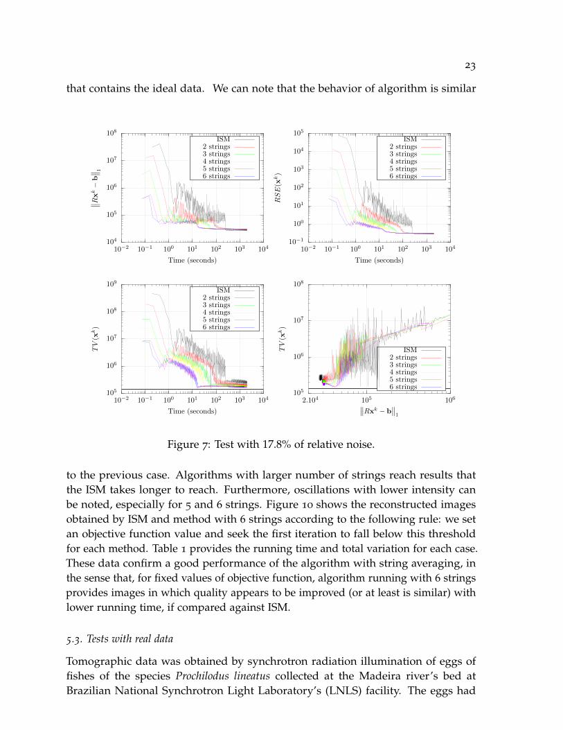
Figure 7: Test with 17.8% of relative noise.
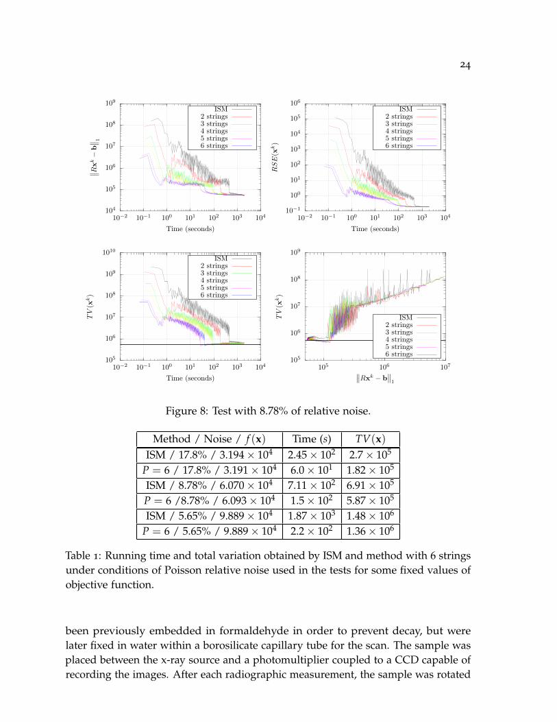
to the previous case. Algorithms with larger number of strings reach results thatthe ISM takes longer to reach. Furthermore, oscillations with lower intensity canbe noted, especially for 5 and 6 strings. Figure 10 shows the reconstructed imagesobtained by ISM and method with 6 strings according to the following rule: we setan objective function value and seek the first iteration to fall below this thresholdfor each method. Table 1 provides the running time and total variation for each case.These data confirm a good performance of the algorithm with string averaging, inthe sense that, for fixed values of objective function, algorithm running with 6 stringsprovides images in which quality appears to be improved (or at least is similar) withlower running time, if compared against ISM.
5.3. Tests with real data
Tomographic data was obtained by synchrotron radiation illumination of eggs offishes of the species Prochilodus lineatus collected at the Madeira river’s bed atBrazilian National Synchrotron Light Laboratory’s (LNLS) facility. The eggs had
24
104
105
106
107
108
109
10−2 10−1 100 101 102 103 104
∥ ∥ Rxk−
b∥ ∥ 1
Time (seconds)
10−1
100
101
102
103
104
105
106
10−2 10−1 100 101 102 103 104
RSE(x
k)
Time (seconds)
105
106
107
108
109
1010
10−2 10−1 100 101 102 103 104
TV(x
k)
Time (seconds)
105
106
107
108
109
105 106 107
TV(x
k)
∥∥Rxk − b∥∥1
ISM2 strings3 strings4 strings5 strings6 strings
ISM2 strings3 strings4 strings5 strings6 strings
ISM2 strings3 strings4 strings5 strings6 strings
ISM2 strings3 strings4 strings5 strings6 strings
Figure 8: Test with 8.78% of relative noise.
Method / Noise / f (x) Time (s) TV(x)ISM / 17.8% / 3.194× 10⁴ 2.45× 10² 2.7× 10⁵
P = 6 / 17.8% / 3.191× 10⁴ 6.0× 101 1.82× 10⁵
ISM / 8.78% / 6.070× 10⁴ 7.11× 10² 6.91× 10⁵
P = 6 /8.78% / 6.093× 10⁴ 1.5× 10² 5.87× 10⁵
ISM / 5.65% / 9.889× 10⁴ 1.87× 10³ 1.48× 10⁶
P = 6 / 5.65% / 9.889× 10⁴ 2.2× 10² 1.36× 10⁶
Table 1: Running time and total variation obtained by ISM and method with 6 stringsunder conditions of Poisson relative noise used in the tests for some fixed values ofobjective function.
been previously embedded in formaldehyde in order to prevent decay, but werelater fixed in water within a borosilicate capillary tube for the scan. The sample wasplaced between the x-ray source and a photomultiplier coupled to a CCD capable ofrecording the images. After each radiographic measurement, the sample was rotated
25
104
105
106
107
108
109
1010
10−2 10−1 100 101 102 103 104
∥ ∥ Rxk−b∥ ∥ 1
Time (seconds)
10−2
10−1
100101102103104105106107108
10−2 10−1 100 101 102 103 104
RSE(x
k)
Time (seconds)
106
107
108
109
1010
1011
10−2 10−1 100 101 102 103 104
TV(x
k)
Time (seconds)
106
107
108
109
105 106 107 108
TV(x
k)
∥∥Rxk − b∥∥1
ISM2 strings3 strings4 strings5 strings6 strings
ISM2 strings3 strings4 strings5 strings6 strings
ISM2 strings3 strings4 strings5 strings6 strings
ISM2 strings3 strings4 strings5 strings6 strings
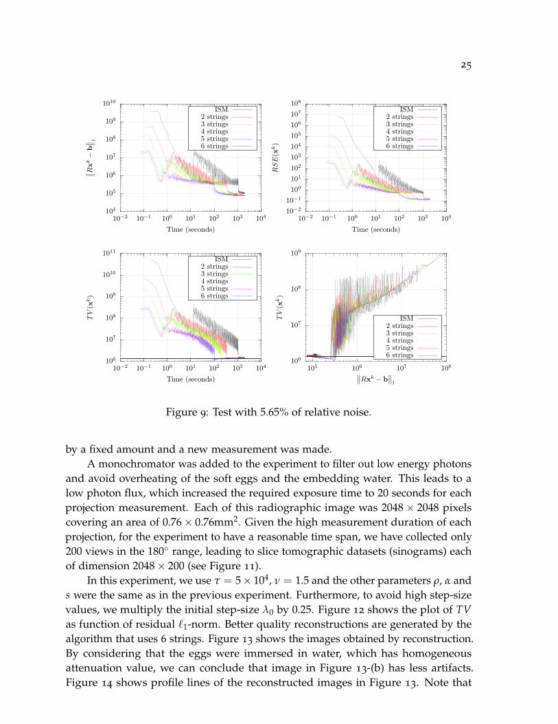
Figure 9: Test with 5.65% of relative noise.
by a fixed amount and a new measurement was made.A monochromator was added to the experiment to filter out low energy photons
and avoid overheating of the soft eggs and the embedding water. This leads to alow photon flux, which increased the required exposure time to 20 seconds for eachprojection measurement. Each of this radiographic image was 2048× 2048 pixelscovering an area of 0.76× 0.76mm2. Given the high measurement duration of eachprojection, for the experiment to have a reasonable time span, we have collected only200 views in the 180◦ range, leading to slice tomographic datasets (sinograms) eachof dimension 2048× 200 (see Figure 11).
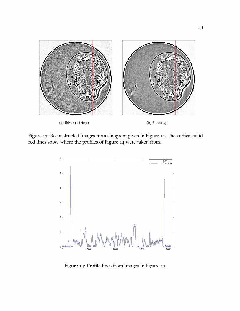
In this experiment, we use τ = 5× 10⁴, ν = 1.5 and the other parameters ρ, α ands were the same as in the previous experiment. Furthermore, to avoid high step-sizevalues, we multiply the initial step-size λ0 by 0.25. Figure 12 shows the plot of TVas function of residual `1-norm. Better quality reconstructions are generated by thealgorithm that uses 6 strings. Figure 13 shows the images obtained by reconstruction.By considering that the eggs were immersed in water, which has homogeneousattenuation value, we can conclude that image in Figure 13-(b) has less artifacts.Figure 14 shows profile lines of the reconstructed images in Figure 13. Note that
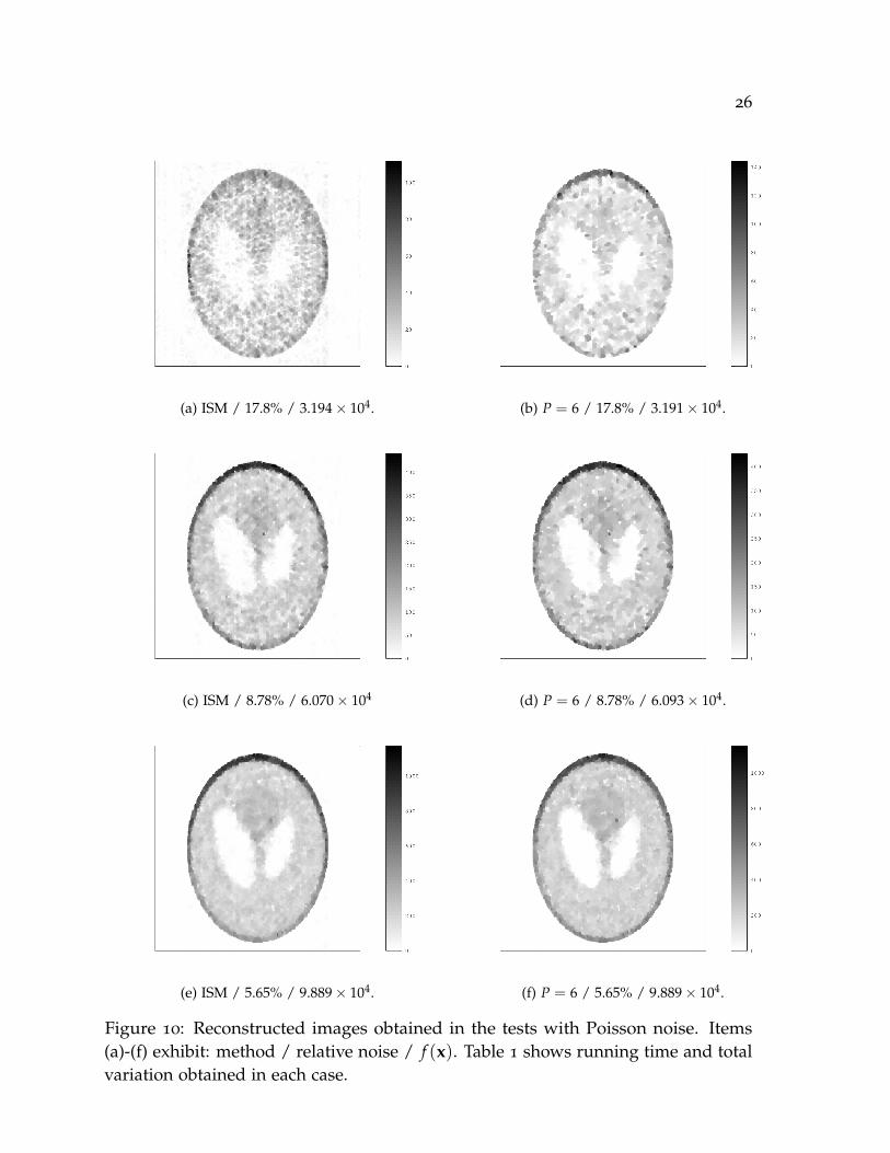
26
(a) ISM / 17.8% / 3.194× 10⁴. (b) P = 6 / 17.8% / 3.191× 10⁴.
(c) ISM / 8.78% / 6.070× 10⁴ (d) P = 6 / 8.78% / 6.093× 10⁴.
(e) ISM / 5.65% / 9.889× 10⁴. (f) P = 6 / 5.65% / 9.889× 10⁴.
Figure 10: Reconstructed images obtained in the tests with Poisson noise. Items(a)-(f) exhibit: method / relative noise / f (x). Table 1 shows running time and totalvariation obtained in each case.
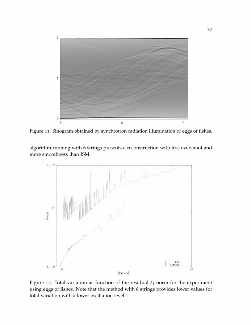
27
Figure 11: Sinogram obtained by synchrotron radiation illumination of eggs of fishes.
algorithm running with 6 strings presents a reconstruction with less overshoot andmore smoothness than ISM.
3 × 10⁶
106
2 × 10⁵
104 105
TV(x
k )
∥∥∥Rxk − b∥∥∥
1
ISM6 strings
Figure 12: Total variation as function of the residual `1-norm for the experimentusing eggs of fishes. Note that the method with 6 strings provides lower values fortotal variation with a lower oscillation level.
28
(a) ISM (1 string) (b) 6 strings
Figure 13: Reconstructed images from sinogram given in Figure 11. The vertical solidred lines show where the profiles of Figure 14 were taken from.
0
1
2
3
4
5
6
0 500 1000 1500 2000
ISM6 strings
Figure 14: Profile lines from images in Figure 13.
REFERENCES 29
6. Final comments
We have presented a new String-Averaging Incremental Subgradients family ofalgorithms. The theoretical convergence analysis of the method was established andexperiments were performed in order to assess the effectiveness of the algorithm. Themethod featured a good performance in practice, being able to reconstruct imageswith superior quality when compared to classical incremental subgradient algorithms.Furthermore, algorithmic parameters selection was shown to be robust across a rangeof tomographic experiments. The discussed theory involves solving non-smoothconstrained convex optimization problems and, in this sense, more general modelscan be numerically addressed by the presented method. Future work may be relatedto the application of the string-averaging technique in incremental subgradientalgorithms with stochastic errors, such as those that appear in [50] and [51].
Acknowledgements
We would like to thank the LNLS for providing the beam time for the tomographicacquisition, obtained under proposal number 17338. We also want to thank Prof.Marcelo dos Anjos (Federal University of Amazonas) for kindly providing the fishegg samples used in the presented experimentation. RMO was partially fundedby FAPESP Grant 2015/10171-2. ESH was partially funded by FAPESP Grants2013/16508-3 and 2013/07375-0 and CNPq Grant 311476/2014-7. EFC was fundedby FAPESP under Grant 13/19380-8 and CNPq under Grant 311290/2013-2.
References
[1] Ahn, S., and Fessler, J. A. Globally convergent image reconstruction foremission tomography using relaxed ordered subsets algorithms. Medical Imaging,IEEE Transactions on 22, 5 (2003), 613–626.
[2] Anthoine, S., Aujol, J.-F., Boursier, Y., and Melot, C. Some proximal methodsfor Poisson intensity CBCT and PET. Inverse Problems and Imaging 6, 4 (2012),565–598.
[3] Bauschke, H. H., and Borwein, J. M. On projection algorithms for solvingconvex feasibility problems. SIAM Review 38, 3 (1996), 367–426.
[4] Bauschke, H. H., Combettes, P. L., and Kruk, S. G. Extrapolation algorithm foraffine-convex feasibility problems. Numerical Algorithms 41, 3 (2006), 239–274.
[5] Beck, A., and Teboulle, M. Fast gradient-based algorithms for constrainedtotal variation image denoising and deblurring problems. IEEE Transactions onImage Processing 18, 11 (2009), 2419–2434.
[6] Beck, A., and Teboulle, M. A fast iterative shrinkage-thresholding algorithmfor linear inverse problems. SIAM Journal on Imaging Sciences 2, 1 (2009), 183–202.
REFERENCES 30
[7] Bertsekas, D. P. A new class of incremental gradient methods for least squaresproblems. SIAM Journal on Optimization 7, 4 (1997), 913–926.
[8] Bertsekas, D. P. Nonlinear programming. Athena scientific, Belmont, MA, 1999.
[9] Bertsekas, D. P., and Tsitsiklis, J. N. Gradient convergence in gradientmethods with errors. SIAM Journal on Optimization 10, 3 (2000), 627–642.
[10] Blatt, D., Hero, A. O., and Gauchman, H. A convergent incremental gradientmethod with a constant step size. SIAM Journal on Optimization 18, 1 (2007),29–51.
[11] Bredies, K. A forward-backward splitting algorithm for the minimization ofnon-smooth convex functionals in Banach space. Inverse Problems 25, 1 (2009),015005.
[12] Browne, J., and De Pierro, A. R. A row-action alternative to the EM algorithmfor maximizing likelihoods in emission tomography. Medical Imaging, IEEETransactions on 15, 5 (1996), 687–699.
[13] Censor, Y., Elfving, T., and Herman, G. T. Averaging strings of sequentialiterations for convex feasibility problems. Inherently parallel algorithms in feasibilityand optimization and their applications 8 (2001), 101–113.
[14] Censor, Y., and Tom, E. Convergence of string-averaging projection schemesfor inconsistent convex feasibility problems. Optimization Methods & Software 18(2003), 543–554.
[15] Censor, Y., and Zaslavski, A. J. Convergence and perturbation resilience ofdynamic string-averaging projection methods. Computational Optimization andApplications 54, 1 (2013), 65–76.
[16] Censor, Y., and Zaslavski, A. J. String-averaging projected subgradientmethods for constrained minimization. Optimization Methods and Software 29, 3
(2014), 658–670.
[17] Chen, G. H.-G., and Rockafellar, R. T. Convergence rates in forward-backward splitting. SIAM Journal on Optimization 7, 2 (1997), 421–444.
[18] Chouzenoux, E., Jezierska, A., Pesquet, J.-C., and Talbot, H. A majorize-minimize subspace approach for `2 − `0 image regularization. SIAM Journal onImaging Sciences 6, 1 (2013), 563–591.
[19] Chouzenoux, E., Pesquet, J. C., Talbot, H., and Jezierska, A. A memorygradient algorithm for `2-`0 regularization with applications to image restoration.In 2011 18th IEEE International Conference on Image Processing (2011), pp. 2717–2720.
[20] Chouzenoux, E., Zolyniak, F., Gouillart, E., and Talbot, H. A majorize-minimize memory gradient algorithm applied to X-ray tomography. In 2013IEEE International Conference on Image Processing (2013), pp. 1011–1015.
REFERENCES 31
[21] Combettes, P. L. Inconsistent signal feasibility problems: Least-squares solutionsin a product space. Signal Processing, IEEE Transactions on 42, 11 (1994), 2955–2966.
[22] Combettes, P. L. Convex set theoretic image recovery by extrapolated iterationsof parallel subgradient projections. Image Processing, IEEE Transactions on 6, 4
(1997), 493–506.
[23] Combettes, P. L., and Pesquet, J.-C. A proximal decomposition method forsolving convex variational inverse problems. Inverse Problems 24, 6 (2008), 065014.
[24] Combettes, P. L., and Pesquet, J.-C. Fixed-Point Algorithms for Inverse Problemsin Science and Engineering. Springer New York, New York, NY, 2011, ch. ProximalSplitting Methods in Signal Processing, pp. 185–212.
[25] Combettes, P. L., and Pesquet, J.-C. Stochastic approximations andperturbations in forward-backward splitting for monotone operators. Pureand Applied Functional Analysis 1, 1 (2016), 13–37.
[26] De Pierro, A. R., and Yamagishi, M. E. B. Fast EM-like methods formaximum “a posteriori” estimates in emission tomography. Medical Imaging,IEEE Transactions on 20, 4 (2001), 280–288.
[27] Dem’yanov, V. F., and Vasil’ev, L. V. Nondifferentiable optimization. Springer,1985.
[28] Dewaraja, Y. K., Koral, K. F., and Fessler, J. A. Regularized reconstruction inquantitative SPECT using CT side information from hybrid imaging. Physics inMedicine and Biology 55, 9 (2010), 2523.
[29] Harmany, Z. T., Marcia, R. F., and Willett, R. M. This is SPIRAL-TAP:Sparse Poisson Intensity Reconstruction Algorithms - theory and practice. IEEETransactions on Image Processing 21, 3 (2012), 1084–1096.
[30] Helou, E. S., Censor, Y., Chen, T.-B., Chern, I.-L., De Pierro, Á. R., Jiang,M., and Lu, H. H.-S. String-averaging expectation-maximization for maximumlikelihood estimation in emission tomography. Inverse Problems 30, 5 (2014),055003.
[31] Herman, G. T. Fundamentals of computerized tomography: image reconstruction fromprojections. Advances in Computer Vision and Pattern Recognition. Springer-Verlag London, 2009.
[32] Hiriart-Urruty, J.-B., and Lemaréchal, C. Convex Analysis and MinimizationAlgorithms I and II. A Series of Comprehensive Studies in Mathematics. Springer-Verlag, Berlin, 1993.
[33] Hoffmann, A. The distance to the intersection of two convex sets expressed bythe distances to each of them. Mathematische Nachrichten 157, 1 (1992), 81–98.
[34] Hudson, H. M., and Larkin, R. S. Accelerated image reconstruction usingordered subsets of projection data. Medical Imaging, IEEE Transactions on 13, 4
(1994), 601–609.
REFERENCES 32
[35] Johansson, B., Rabi, M., and Johansson, M. A randomized incrementalsubgradient method for distributed optimization in networked systems. SIAMJournal on Optimization 20, 3 (2010), 1157–1170.
[36] Kak, A. C., and Slaney, M. Principles of Computerized Tomographic Imaging. IEEEpress, 1988.
[37] Kibardin, V. M. Decomposition into functions in the minimization problem.Avtomatika i Telemekhanika, 9 (1979), 66–79.
[38] Natterer, F. The Mathematics of Computerized Tomography. Wiley, 1986.
[39] Natterer, F., and Wübbeling, F. Mathematical methods in image reconstruction.SIAM, 2001.
[40] Nedic, A., and Bertsekas, D. P. Incremental subgradient methods fornondifferentiable optimization. SIAM Journal on Optimization 12, 1 (2001), 109–138.
[41] Neto, E. S. H., and De Pierro, A. R. Convergence results for scaled gradientalgorithms in positron emission tomography. Inverse problems 21 (2005), 1905.
[42] Neto, E. S. H., and De Pierro, Á. R. Incremental subgradients for constrainedconvex optimization: a unified framework and new methods. SIAM Journal onOptimization 20, 3 (2009), 1547–1572.
[43] Penfold, S. N., Schulte, R. W., Censor, Y., Bashkirov, V., McAllister, S.,Schubert, K. E., and Rosenfeld, A. B. Block-iterative and string-averagingprojection algorithms in proton computed tomography image reconstruction.Biomedical Mathematics: Promising Directions in Imaging, Therapy Planning andInverse Problems (2010), 347–367.
[44] Polyak, B. T. Introduction to optimization. 1987. Optimization Software, Inc, NewYork.
[45] Raguet, H., Fadili, J., and Peyré, G. A generalized forward-backward splitting.SIAM Journal on Imaging Sciences 6, 3 (2013), 1199–1226.
[46] Shepp, L. A., and Vardi, Y. Maximum likelihood reconstruction for emissiontomography. Medical Imaging, IEEE Transactions on 1, 2 (1982), 113–122.
[47] Shor, N. Z. Minimization methods for non-differentiable functions. Springer-VerlagNew York, Inc., 1985.
[48] Solodov, M. V. Incremental gradient algorithms with stepsizes bounded awayfrom zero. Computational Optimization and Applications 11, 1 (1998), 23–35.
[49] Solodov, M. V., and Zavriev, S. K. Error stability properties of generalizedgradient-type algorithms. Journal of Optimization Theory and Applications 98, 3
(1998), 663–680.
[50] Sundhar Ram, S., Nedic, A., and Veeravalli, V. V. Incremental stochasticsubgradient algorithms for convex optimization. SIAM Journal on Optimization20, 2 (2009), 691–717.
REFERENCES 33
[51] Sundhar Ram, S., Nedic, A., and Veeravalli, V. V. Distributed stochasticsubgradient projection algorithms for convex optimization. Journal of optimizationtheory and applications 147, 3 (2010), 516–545.
[52] Tanaka, E., and Kudo, H. Subset-dependent relaxation in block-iterativealgorithms for image reconstruction in emission tomography. Physics in medicineand biology 48, 10 (2003), 1405.
[53] Tseng, P. An incremental gradient (-projection) method with momentum termand adaptive stepsize rule. SIAM Journal on Optimization 8, 2 (1998), 506–531.
[54] Vardi, Y., Shepp, L., and Kaufman, L. A statistical model for positron emissiontomography. Journal of the American Statistical Association 80, 389 (1985), 8–20.
[55] Yamada, I., and Ogura, N. Adaptive projected subgradient method forasymptotic minimization of sequence of nonnegative convex functions. NumericalFunctional Analysis and Optimization 25, 7 (2005), 593–617.
[56] Yamada, I., and Ogura, N. Hybrid steepest descent method for variationalinequality problem over the fixed point set of certain quasi-nonexpansivemappings. Numerical Functional Analysis and Optimization 25, 7 (2005), 619–655.