Contents lists available at ScienceDirect

Journal of the Mechanics and Physics of Solids

Journal of the Mechanics and Physics of Solids 96 (2016) 445–459

http://d0022-50

n CorrE-m

journal homepage: www.elsevier.com/locate/jmps

On poro-hyperelastic shear

A.P. Suvorov, A.P.S. Selvadurai n

Department of Civil Engineering and Applied Mechanics McGill University, 817 Sherbrooke Street West, Montréal, QC, Canada H3A0C3

a r t i c l e i n f o

Article history:Received 28 June 2016Accepted 8 August 2016Available online 10 August 2016

Keywords:Poro-hyperelasticityFluid-saturated mediaCanonical analytical solutionsLarge deformationsTime-dependent phenomenaCalibration of computational results

x.doi.org/10.1016/j.jmps.2016.08.00696/& 2016 Elsevier Ltd. All rights reserved.

esponding author.ail address: patrick.selvadurai@mcgill.ca (A.P

a b s t r a c t

The paper examines the problem of the shear of a porous hyperelastic material, the porespace of which is saturated with an incompressible fluid. Poro-hyperelasticity provides asuitable approach for modelling the mechanical behaviour of highly deformable materialsin engineering applications and particularly soft tissues encountered in biomechanicalapplications. Unlike with the infinitesimal theory of poroelasticity, the application of pureshear generates pore fluid pressures that dissipate with time as fluid migrates either fromor into the pore space due to the generated fluid pressure gradients. The analytical resultsprovide benchmark problems that can be used to examine the accuracy of computationalapproaches.

& 2016 Elsevier Ltd. All rights reserved.

1. Introduction

The mechanics of a fluid saturated porous medium is largely associated with the study of consolidation of geomaterialsundergoing small deformations. Although several researchers in the field of geomechanics have examined one-dimensionalproblems in the theory of soil consolidation, the rigorous development of a mathematically consistent theory of por-oelasticity was first proposed by Biot (1941). The theory considers the three-dimensional development of the topic wherethe elastic behaviour of the porous skeleton is defined by Hooke's law, the migration of fluid within the accessible porespace is defined by Darcy's law, and the partition of the total stresses to the stresses sustained by the porous skeleton andthe pore fluid takes into consideration the compatibility of volume changes between the two phases. Since these earlydevelopments, the classical theory of poroelasticity has been widely applied in a number of areas including geomechanics,biomechanics and materials science. The number of articles covering the applications of the classical theory of poroelasticityto these topics is far too numerous to cite individually; comprehensive accounts are given by Selvadurai (2006, 2007, 2015),Cheng (2016), Selvadurai and Suvorov (2016a, 2016b) and in proceedings of regularly organized conferences devoted to BiotPoromechanics. These articles contain references to important contributions to poromechanics and hyperelasticity. Ofparticular relevance is the recent article by Selvadurai and Suvorov (2016a) that contains in excess of 160 references ger-mane to the modelling of hyperelastic materials, developments in the mechanics of multi-phasic materials, analytical so-lutions to certain canonical problems of poro-hyperelasticity and comparisons with computational simulations of the same.

The constraints of the infinitesimal theory restrict the application of the classical theory of poroelasticity to situationswhere the medium experiences large strains. The classical theory of poroelasticity was extended by Biot (1972) to includefinite strains but the application of the approach has not progressed beyond this initial development. Due to the increasedfocus in recent years on modelling soft tissues encountered in biological and medical sciences and highly deformable porous

.S. Selvadurai).

A.P. Suvorov, A.P.S. Selvadurai / J. Mech. Phys. Solids 96 (2016) 445–459446

materials in tactile sensor applications (here the fluid is air), there have been concerted efforts to incorporate modelling ofsuch materials by appeal to classical theories of hyperelasticity, generally without considering the influence of the pore fluidpressure and its diffusive effects encountered in the coupled poro-hyperelasticity problem. In this paper, the studies ofSelvadurai and Suvorov (2016a) are extended to examine the classical problem of the shearing of a fluid-saturated hyper-elastic material, with a specified form of a strain energy function. The boundaries of the region under shear are hydraulicallyconstrained to initiate one-dimensional fluid flow in the deformed region. The mathematical solutions are complementedby computational results obtained via a finite element technique.

2. Constitutive modelling

We consider the total Cauchy stress σij in the fluid-saturated poro-hyperelastic material, which is assumed to be com-posed of the Cauchy stress relevant to the porous hyperelastic fabric (σ′ij) and the isotropic stress in the interstitial fluids,denoted by p. We consider the effective stress relationship of the form

σ σ δ= ′ − ( )p , 2.1ij ij ij

where δij is the Kronecker delta. This form of the effective stress relationship for the fluid-saturated hyperelastic material isan adaptation of the relationship proposed in soil mechanics literature and a limiting case of the result developed by Biot(1941), which takes into consideration the compressibilities of both the pore fluid and the porous skeleton. In the limitingcase when the compressibility of the porous skeleton is small in comparison to the compressibility of the pore fluid, Biot'sresult reduces to Eq. (2.1). The effective or skeletal stress σ′ij can be represented in terms of its deviatoric component ′s ij andan isotropic stress (effective pressure) ′p such that

σ δ σ′ = ′ − ′ ′ = − ′ ( )s p p, /3. 2.2ij ij ij ii

We consider the initial coordinates of a point in the deformable porous skeleton denoted by ( = )X i 1, 2, 3i (with= = =X X X Y X Z; ;1 2 3 ), which moves to a new position with coordinates defined by ( = )x i 1, 2, 3i (with = = =x x x y x z; ;1 2 3 ).

The deformation gradient tensor F is given by

= = ∂∂ ( )

fxX

F .2.3ij

i

j

The left Cauchy-Green deformation tensor B is defined by

¯ = ¯ ¯ ( )B FF , 2.4T

where

¯ = = ( )−J JF F F; det . 2.51/3

The strain energy function U for the isotropic hyperelastic material is assumed to be of the form

= (¯ ¯ ) ( )U U I I J, , 2.61 2

where I1 and I2 are, respectively, the first and second invariants of the strain tensor B. The deviatoric component of theeffective stress ′s is defined as

′ = ∂∂¯ + ¯ ∂

∂¯¯ − ∂

∂¯¯ ⋅ ¯

( )

⎧⎨⎩⎛⎝⎜

⎞⎠⎟

⎫⎬⎭Jdev

UI

IUI

UI

s B B B2

.2.71

12 2

The isotropic component of the effective stress is defined as

′ = − ∂∂ ( )

pUJ

.2.8

Extensive discussions of the various forms of strain energy functions that have been proposed in the literature to de-scribe hyperelastic materials are given by Rivlin (1960), Spencer (1970), Green and Adkins (1970), Lur’e (1990) (see alsoSelvadurai (2006); Selvadurai and Suvorov (2016a) for further references). In this work we consider the finite deformationproblem, which is formulated with reference to a second-order reduced polynomial constitutive model, which is defined as

= (¯ − ) + (¯ − ) + ( − ) + ( − )( )

U C I C ID

JD

J3 31

11

1 ,2.910 1 20 1

2

1

2

2

4

where C10, C20, D1 and D2 are material parameters. We note that in the strain energy function Eq. (2.9) the terms containingstrain invariants I1, I2 are uncoupled from the terms containing the strain invariant J , which implies that there is no couplingbetween shear and volumetric deformations. The constants C10 and D1 can be defined in terms of the linear elastic shearmodulus ( )G and the bulk modulus ( )K of the porous fabric as

A.P. Suvorov, A.P.S. Selvadurai / J. Mech. Phys. Solids 96 (2016) 445–459 447

= = ( )C G DK

2 ,2

. 2.1010 1

For this particular material, the deviatoric component of the effective stress is given by

( )′ = [ + (¯ − )] ¯ ¯( )J

C C Is FF2

2 3 dev ,2.11

T10 20 1

and the isotropic component of the effective stress (effective pressure) can be expressed in the form

′ = − ( − ) − ( − )( )

pD

JD

J2

14

1 .2.121 2

3

If =C 020 , → ∞D2 , the strain energy function for the neoHookean material can be recovered from Eq. (2.9).To complete the constitutive modelling, we need to consider fluid flow through a poro-hyperelastic material. Attention is

restricted to the case where the entire pore space of the hyperelastic skeleton is saturated with a fluid and we assume thatfluid flow takes place as a result of a gradient in the Bernoulli potential. In the case of slow flows through the pore space, thevelocity potential can be neglected in comparison to the other contributions and the datum potential can also be neglectedprovided that the potential is measured with reference to a fixed datum (Selvadurai, 2000).

Considering the principle of mass conservation, we have

ϕ−∇⋅ ( − ) = ∇⋅ ∂∂ ( )t

v vu

2.13f s

where ϕ is the porosity, vf is the velocity of the fluid in the pore space and vs is the velocity of the solid skeleton of theporous material, ∇ is the gradient operator referred to the coordinates of a particle of fluid in the deformed configuration,and u is the displacement vector defined as = −u x X. The derivation of Eq. (2.13) is presented in Selvadurai and Suvorov(2016a) and will not be repeated here.

We assume that flow of the fluid through the isotropic hyperelastic skeleton can be described by an isotropic form ofDarcy's law as

φη

( − ) = − ∇( )

kpv v ,

2.14f s

where k is the permeability, which is assumed to be a constant, and η is the dynamic fluid viscosity. We note that whenporous hyperelastic media are subjected to large strains, the porosity will change with the strain and the permeability willevolve with the alteration of porosity. In this study, however, we do not attempt to introduce the strain dependency in theporosity and consequently the permeability of the porous hyperelastic material remains constant.

By combining Eqs. (2.13) and (2.14) we can obtain the governing equation for the fluid pressure

η∇ = ∇⋅ ∂

∂ ( )k

ptu

.2.15

2

In Eq. (2.15) ∇2 is Laplace's operator referred to the coordinates in the deformed configuration, i.e.,

∇ = ∂∂

+ ∂∂

+ ∂∂ ( )x y z

.2.16

22

2

2

2

2

2

Using the familiar chain rule for differentiation, the second derivatives of Eq. (2.16) can be expressed in terms of deri-vatives with respect to coordinates in the initial configuration. For example,

∂∂

= ∂∂

∂∂

+ ∂∂

∂∂

+ ∂∂

∂∂

+ ∂∂ ∂

∂∂

∂∂

+ ∂∂ ∂

∂∂

∂∂

+ ∂∂ ∂

∂∂

∂∂

+ ∂∂

∂∂

+ ∂∂

∂∂

+ ∂∂

∂∂ ( )

⎛⎝⎜

⎞⎠⎟

⎛⎝⎜

⎞⎠⎟

⎛⎝⎜

⎞⎠⎟x X

Xx Y

Yx Z

Zx X Y

Xx

Yx

X ZXx

Zx Y Z

Yx

Zx X

Xx Y

Yx Z

Zx

2

2 2 . 2.17

2

2

2

2

2 2

2

2 2

2

2 2

2 2 2

2

2

2

2

2

3. Problem of instantaneous simple shear deformation

Consider an infinite layer of a poro-hyperelastic material consisting of incompressible solid and fluid phases. It is as-sumed that the strain energy function for the skeletal material under drained conditions corresponds to the strain energy ofa neoHookean material. The initial thickness of the layer is denoted by h (Fig. 1). A uniform shear stress of magnitude τ issuddenly applied as a Heaviside step function of time over the entire upper surface and the normal stress and the pore fluidpressure are maintained at zero. The base of the infinite layer is constrained from movement and considered to beimpermeable.

Fig. 1. Instantaneous response of a poro-hyperelastic layer of infinite extent subjected to shear.

A.P. Suvorov, A.P.S. Selvadurai / J. Mech. Phys. Solids 96 (2016) 445–459448

3.1. Initial response – simple shear deformation

The initial response of the layer is undrained, which implies that there is no loss or gain of the fluid at time =t 0. In turn,this implies that the volume of the deformed layer will be preserved immediately after application of the stress τ ( )tH(where ( )tH is the Heaviside step function), since the constituents of the layer are incompressible (Fig. 1). Therefore, at time

=t 0 the deformed coordinates of the layer can be prescribed as

γ= + = ( )x X Y y Y; 3.10

where γ0 is an initial shear strain that needs to be determined. The displacements are given by

γ= = ( )u Y v; 0 3.20

and the initial deformation gradient is given by

γ=

( )

⎛

⎝⎜⎜⎜

⎞

⎠⎟⎟⎟F

1 0

0 1 00 0 1

.

3.30

0

It is clear that ( ) =Fdet 10 . Consequently, we can evaluate the deformation tensor

γ γ

γ=+

( )

⎛

⎝

⎜⎜⎜

⎞

⎠

⎟⎟⎟B

1 0

1 0

0 0 1

.

3.4

0

02

0

0

Thus, for the neoHookean material the deviatoric effective stress can be expressed as

γ γ

γ γ

γ

′ = −

−( )

⎛

⎝

⎜⎜⎜⎜⎜⎜⎜

⎞

⎠

⎟⎟⎟⎟⎟⎟⎟

Cs 2

23

0

13

0

0 013

.

3.5

10

02

0

0 02

02

and the effective pressure is equal to zero since there is no change in the volume of the material

′ = ( )p 0. 3.6

Therefore, according to Eqs. (2.1) and (2.2), the initial total stress in the layer can be represented by

σ γ

σ γ

σ γ

= −

=

= − −( )

⎧

⎨⎪⎪⎪

⎩⎪⎪⎪

C p

C

C p

432

23 3.7

xx

xy

yy

10 02

0

10 0

10 02

0

where p0 is an initial fluid pressure generated in the layer. To find this fluid pressure and the shear strain, we use the tractionboundary conditions. This gives us

Fig. 2. Long-term response of a poro-hyperelastic layer of infinite extent subjected to shear.

A.P. Suvorov, A.P.S. Selvadurai / J. Mech. Phys. Solids 96 (2016) 445–459 449

γ τ γ τ= = − = −( )C

p CC2

;23 6

.3.80

100 10 0

22

10

Thus, the initial fluid pressure is negative.

3.2. Long-term response

In the long-term, the fluid pressure in the porous layer will dissipate to zero. The deformation gradient can be re-presented by

γε= +

( )

⎛

⎝⎜⎜⎜

⎞

⎠⎟⎟⎟F

1 0

0 1 00 0 1 3.9

1

1

1

where γ1 is a final shear strain and ε1 is a final axial strain of the layer (Fig. 2). Note that unlike the initial deformationgradient Eq. (3.3) the deformation gradient Eq. (3.9) does not correspond to a state of simple shear deformation (Fig. 2); Eq.(3.9) results from a superposition of a shear deformation with uniaxial deformation in the thickness direction. The de-terminant of Eq. (3.9) is

ε( ) = +Fdet 1 ,1 1

and the deformation tensor can be obtained as

εγ γ ε

γ ε ε¯ = ( + )+ ( + )

( + ) ( + )( )

−

⎛

⎝

⎜⎜⎜

⎞

⎠

⎟⎟⎟B 1

1 1 0

1 1 0

0 0 1 3.10

1 12/3

12

1 1

1 1 12

Consequently, for the neoHookean material, the deviatoric effective stress can be expressed as

ε

γ ε γ ε

γ ε γ ε

γ ε

′ = ( + )

+ − ( + ) ( + )

( + ) − − + ( + )

− − ( + )( )

−

⎛

⎝

⎜⎜⎜⎜⎜⎜⎜

⎞

⎠

⎟⎟⎟⎟⎟⎟⎟

Cs 2 1

13

23

13

1 1 0

123

13

23

1 0

0 013

13

13

13.11

10 15/3

12

12

1 1

1 1 12

12

12

12

and the effective pressure is

ε′ = − ( − ) = − ( )pD

JD

21

2. 3.121

Now, using the traction boundary conditions on the upper surface, we obtain a system of two non-linear algebraicequations to be solved for the unknown strains γ1 and ε1:

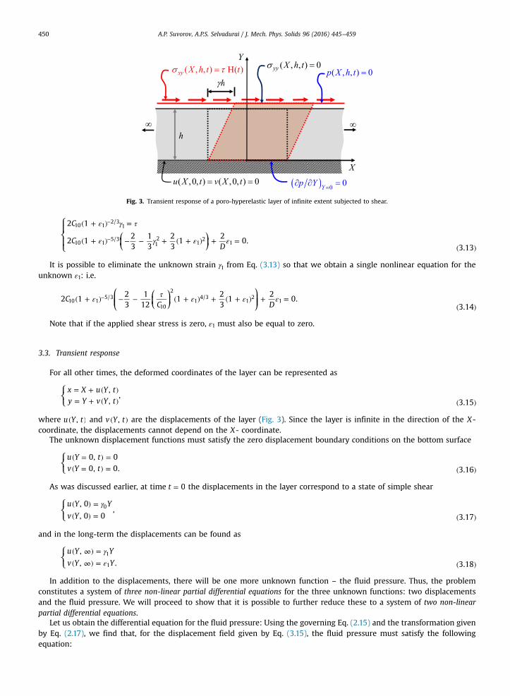
Fig. 3. Transient response of a poro-hyperelastic layer of infinite extent subjected to shear.

A.P. Suvorov, A.P.S. Selvadurai / J. Mech. Phys. Solids 96 (2016) 445–459450

ε γ τ

ε γ ε ε

( + ) =

( + ) − − + ( + ) + =( )

−

−

⎧⎨⎪

⎩⎪⎛⎝⎜

⎞⎠⎟

C

CD

2 1

2 123

13

23

12

0.3.13

10 12/3

1

10 15/3

12

12

1

It is possible to eliminate the unknown strain γ1 from Eq. (3.13) so that we obtain a single nonlinear equation for theunknown ε1: i.e.

ε τ ε ε ε( + ) − − ( + ) + ( + ) + =( )

−⎛⎝⎜⎜

⎛⎝⎜

⎞⎠⎟

⎞⎠⎟⎟C

C D2 1

23

112

123

12

0.3.14

10 15/3

10

2

14/3

12

1

Note that if the applied shear stress is zero, ε1 must also be equal to zero.

3.3. Transient response

For all other times, the deformed coordinates of the layer can be represented as

= + ( )= + ( ) ( )

⎧⎨⎩x X u Y ty Y v Y t

,,

,3.15

where ( )u Y t, and ( )v Y t, are the displacements of the layer (Fig. 3). Since the layer is infinite in the direction of the X-coordinate, the displacements cannot depend on the X- coordinate.

The unknown displacement functions must satisfy the zero displacement boundary conditions on the bottom surface

( = ) =( = ) = ( )

⎧⎨⎩u Y t

v Y t

0, 00, 0. 3.16

As was discussed earlier, at time =t 0 the displacements in the layer correspond to a state of simple shear

γ( ) =( ) = ( )

⎧⎨⎩u Y Y

v Y

, 0

, 0 0,

3.170

and in the long-term the displacements can be found as

γε

( ∞) =( ∞) = ( )

⎧⎨⎩u Y Y

v Y Y

,

, . 3.181

1

In addition to the displacements, there will be one more unknown function – the fluid pressure. Thus, the problemconstitutes a system of three non-linear partial differential equations for the three unknown functions: two displacementsand the fluid pressure. We will proceed to show that it is possible to further reduce these to a system of two non-linearpartial differential equations.

Let us obtain the differential equation for the fluid pressure: Using the governing Eq. (2.15) and the transformation givenby Eq. (2.17), we find that, for the displacement field given by Eq. (3.15), the fluid pressure must satisfy the followingequation:

A.P. Suvorov, A.P.S. Selvadurai / J. Mech. Phys. Solids 96 (2016) 445–459 451

η η∂∂

∂∂

+ ∂∂

+ ∂∂

∂∂

+ ∂∂

= ∂∂ ∂

∂∂

+ ∂∂ ∂

∂∂ ( )

⎛⎝⎜⎜

⎛⎝⎜

⎞⎠⎟

⎛⎝⎜

⎞⎠⎟

⎞⎠⎟⎟

⎛⎝⎜

⎞⎠⎟

k pY

Yx

Yy

k pY

Yx

Yy

uY t

Yx

vY t

Yy

,3.19

2

2

2 2 2

2

2

2

2 2

since the fluid pressure and the displacements are independent of the X- coordinate.However, from Eq. (3.15) it follows that

∂∂

= ∂∂

= + ∂∂ ( )

−⎜ ⎟⎛⎝

⎞⎠

Yx

Yy

vY

0; 1 .3.20

1

Therefore,

∂∂

= − ∂∂

+ ∂∂ ( )

−⎜ ⎟⎛⎝

⎞⎠

Yy

vY

vY

13.21

2

2

2

2

3

and, consequently, Eq. (3.19) is reduced to

η η∂∂

+ ∂∂

− ∂∂

∂∂

+ ∂∂

= ∂∂ ∂ ( )

− −⎜ ⎟ ⎜ ⎟⎛⎝

⎞⎠

⎛⎝

⎞⎠

k pY

vY

k pY

vY

vY

vY t

1 1 .3.22

2

2

1 2

2

2 2

Since the upper surface of the layer is drained and the lower surface is impervious, the boundary conditions for the fluidpressure can be written as

( ) = ∂∂

( ) = ( )p h tpY

t, 0; 0, 0. 3.23

At time =t 0 the fluid pressure is known and is given by Eq. (3.8)

γ τ= − = −( ′ )

p CC

23 6

.3. 80 10 0

22

10

The stress components and equilibrium equations can then be obtained. The deformation gradient is given by

=

∂∂

+ ∂∂

( )

⎛

⎝

⎜⎜⎜⎜⎜

⎞

⎠

⎟⎟⎟⎟⎟

uY

vY

F

1 0

0 1 0

0 0 1

,

3.24

and therefore,

¯ =

∂∂

+ ∂∂

= + ∂∂

( )

−

⎛

⎝

⎜⎜⎜⎜⎜

⎞

⎠

⎟⎟⎟⎟⎟J

uY

vY

JvY

F

1 0

0 1 0

0 0 1

; 1 .

3.25

1/3

The deformation tensor is given by

¯ =

+ ∂∂

∂∂

( + ∂∂

)

∂∂

+ ∂∂

+ ∂∂

( )

−

⎜ ⎟

⎜ ⎟ ⎜ ⎟

⎛

⎝

⎜⎜⎜⎜⎜⎜

⎛⎝

⎞⎠

⎛⎝

⎞⎠

⎛⎝

⎞⎠

⎞

⎠

⎟⎟⎟⎟⎟⎟J

uY

uY

vY

uY

vY

vY

B

1 1 0

1 1 0

0 0 1

.

3.26

2/3

2

2

Consequently, for the neoHookean material, the deviatoric effective stress can be obtained as

′ =

+ ∂∂

− + ∂∂

∂∂

+ ∂∂

∂∂

+ ∂∂

− − ∂∂

+ + ∂∂

− ∂∂

− + ∂∂ ( )

−

⎜ ⎟ ⎜ ⎟ ⎜ ⎟

⎜ ⎟ ⎜ ⎟ ⎜ ⎟

⎜ ⎟ ⎜ ⎟

⎛

⎝

⎜⎜⎜⎜⎜⎜⎜⎜

⎛⎝

⎞⎠

⎛⎝

⎞⎠

⎛⎝

⎞⎠

⎛⎝

⎞⎠

⎛⎝

⎞⎠

⎛⎝

⎞⎠

⎛⎝

⎞⎠

⎛⎝

⎞⎠

⎞

⎠

⎟⎟⎟⎟⎟⎟⎟⎟

C J

uY

vY

uY

vY

uY

vY

uY

vY

uY

vY

s 2

13

23

13

1 1 0

123

13

23

1 0

0 013

13

13

13.27

105/3

2 2

2 2

2 2

and the effective pressure is

A.P. Suvorov, A.P.S. Selvadurai / J. Mech. Phys. Solids 96 (2016) 445–459452

′ = − ( − ) = − ∂∂ ( )p

DJ

DvY

21

2. 3.28

Therefore, the individual components of the effective stress tensor are given by

σ

σ

σ

′ = + ∂∂

+ ∂∂

− + ∂∂

+ ∂∂

′ = + ∂∂

∂∂

′ = + ∂∂

− − ∂∂

+ + ∂∂

+ ∂∂ ( )

−

−

−

⎜ ⎟ ⎜ ⎟ ⎜ ⎟

⎜ ⎟

⎜ ⎟ ⎜ ⎟ ⎜ ⎟

⎧

⎨

⎪⎪⎪⎪

⎩

⎪⎪⎪⎪

⎛⎝

⎞⎠

⎛⎝⎜

⎛⎝

⎞⎠

⎛⎝

⎞⎠

⎞⎠⎟

⎛⎝

⎞⎠

⎛⎝

⎞⎠

⎛⎝⎜

⎛⎝

⎞⎠

⎛⎝

⎞⎠

⎞⎠⎟

CvY

uY

vY D

vY

CvY

uY

CvY

uY

vY D

vY

2 113

23

13

12

2 1

2 123

13

23

12

,

3.29

xx

xy

yy

10

5/3 2 2

10

2/3

10

5/3 2 2

and thus, the traction boundary conditions on the upper surface can be written as

τ+ ∂∂

∂∂

=

+ ∂∂

− − ∂∂

+ + ∂∂

+ ∂∂

==

( )

−

−

⎜ ⎟

⎜ ⎟ ⎜ ⎟ ⎜ ⎟

⎧

⎨⎪⎪

⎩⎪⎪

⎛⎝

⎞⎠

⎛⎝

⎞⎠

⎛⎝⎜

⎛⎝

⎞⎠

⎛⎝

⎞⎠

⎞⎠⎟

CvY

uY

CvY

uY

vY D

vY

Y h

2 1

2 123

13

23

12

0, .

3.30

10

2/3

10

5/3 2 2

In the deformed configuration, the equations of equilibrium governing the Cauchy stresses can be written as

σ σ

σ σ

∂ ′∂

+∂ ′

∂− ∂

∂=

∂ ′∂

+∂ ′

∂− ∂

∂=

( )

⎧⎨⎪⎪

⎩⎪⎪

x ypx

x ypy

0

0.3.31

xx xy

xy yy

Using the chain rule for differentiation and noting that ( )∂ ∂ =Y x/ 0, the system of Eq. (3.31) can be re-written as

σ

σ

∂ ′∂

+ ∂∂

=

∂ ′∂

+ ∂∂

− ∂∂

+ ∂∂

=( )

−

− −

⎜ ⎟

⎜ ⎟ ⎜ ⎟

⎧⎨⎪⎪

⎩⎪⎪

⎛⎝

⎞⎠

⎛⎝

⎞⎠

⎛⎝

⎞⎠

YvY

YvY

pY

vY

1 0

1 1 0

,

3.32

xy

yy

1

1 1

or

σ

σ

∂ ′∂

=

∂ ′∂

− ∂∂

=( )

⎧⎨⎪⎪

⎩⎪⎪

Y

YpY

0

0.3.33

xy

yy

Now using the traction boundary conditions Eq. (3.30), we can obtain two equilibrium equations in the following form

σ τσ

′ ( ) =′ ( ) − ( ) = ( )

⎪

⎪⎧⎨⎩

Y

Y p Y 0. 3.34

xy

yy

Consequently, using expressions Eq. (3.29),

τ+ ∂∂

∂∂

=

+ ∂∂

− − ∂∂

+ + ∂∂

+ ∂∂

− =( )

−

−

⎜ ⎟

⎜ ⎟ ⎜ ⎟ ⎜ ⎟

⎧

⎨⎪⎪

⎩⎪⎪

⎛⎝

⎞⎠

⎛⎝

⎞⎠

⎛⎝⎜

⎛⎝

⎞⎠

⎛⎝

⎞⎠

⎞⎠⎟

CvY

uY

CvY

uY

vY D

vY

p

2 1

2 123

13

23

12

0.3.35

10

2/3

10

5/3 2 2

It is possible to express ( )∂ ∂u Y/ from the first equilibrium equation and substitute it into the second equation. Theresulting equilibrium equation can be written as

τ+ ∂∂

− − + ∂∂

+ + ∂∂

+ ∂∂

− =( )

−⎜ ⎟ ⎜ ⎟ ⎜ ⎟⎛⎝

⎞⎠

⎛⎝⎜⎜

⎛⎝⎜

⎞⎠⎟

⎛⎝

⎞⎠

⎛⎝

⎞⎠

⎞⎠⎟⎟C

vY C

vY

vY D

vY

p2 123

112

123

12

0.3.36

10

5/3

10

2 4/3 2

Therefore, the problem can be reduced to solving two nonlinear partial differential equations for the two unknownfunctions – the fluid pressure p and the vertical displacement v:

A.P. Suvorov, A.P.S. Selvadurai / J. Mech. Phys. Solids 96 (2016) 445–459 453

η η

τ

∂∂

+ ∂∂

− ∂∂

∂∂

+ ∂∂

= ∂∂ ∂

− + ∂∂

− + ∂∂

+ + ∂∂

+ ∂∂

− =( )

− −

− −

⎜ ⎟ ⎜ ⎟

⎜ ⎟ ⎜ ⎟ ⎜ ⎟

⎧

⎨⎪⎪

⎩⎪⎪

⎛⎝

⎞⎠

⎛⎝

⎞⎠

⎛⎝⎜⎜ ⎛

⎝⎞⎠

⎛⎝⎜

⎞⎠⎟

⎛⎝

⎞⎠

⎛⎝

⎞⎠

⎞⎠⎟⎟

k pY

vY

k pY

vY

vY

vY t

CvY C

vY

vY D

vY

p

1 1

223

11

121

23

12

0.3.37

2

2

1 2

2

2 2

10

5/3

10

2 1/3 1/3

Using the notation

ε∂∂

= ( ) ( )vY

Y t, 3.38

we can rewrite the system of Eq. (3.37) as

( )

( ) ( ) ( )

ηε

ηε ε ε

ε τ ε ε ε

∂∂

+ − ∂∂

∂∂

( + ) = ∂∂

− + − + + + + − =( )

− −

− −

⎧

⎨⎪⎪

⎩⎪⎪

⎛⎝⎜⎜

⎛⎝⎜

⎞⎠⎟

⎞⎠⎟⎟

k pY

k pY Y t

CC D

p

1 1

223

11

121

23

12

0.3.39

2

21 2

105/3

10

21/3 1/3

By taking the first and second derivatives of the second Eq. of (3.39) with respect to Y , we obtain

( ) ( ) ( )ε τ ε ε ε ε+ + + + + ∂∂

+ ∂∂

= ∂∂

− − −⎛⎝⎜⎜

⎛⎝⎜

⎞⎠⎟

⎞⎠⎟⎟C

C Y D YpY

2109

11

361

29

12

108/3

10

24/3 2/3

( ) ( ) ( )

( ) ( ) ( )

ε τ ε ε ε

ε τ ε ε ε ε

+ + + + + ∂∂

+

− + − + − + ∂∂

+ ∂∂

= ∂∂

− − −

− − − ⎜ ⎟

⎛⎝⎜⎜

⎛⎝⎜

⎞⎠⎟

⎞⎠⎟⎟

⎛⎝⎜⎜

⎛⎝⎜

⎞⎠⎟

⎞⎠⎟⎟⎛

⎝⎞⎠

CC Y

CC Y D Y

pY

2109

11

361

29

1

28027

11

271

427

12

108/3

10

24/3 2/3

2

2

1011/3

10

27/3 5/3

2 2

2

2

2

By substituting these results into the first equation of the system Eq. (3.39), we obtain

( ) ( ) ( )

( ) ( ) ( )

( ) ( ) ( ) ( )

ε τ ε ε ε

ε τ ε ε ε

ε τ ε ε ε ε η ε ε

+ + + + + + ∂∂

+

− + − + − + ∂∂

− + + + + + + ∂∂

( + ) = + ∂∂ ( )

− − −

− − −

− − − −

⎜ ⎟

⎜ ⎟

⎛⎝⎜⎜

⎛⎝⎜⎜

⎛⎝⎜

⎞⎠⎟

⎞⎠⎟⎟

⎞⎠⎟⎟

⎛⎝⎜⎜

⎛⎝⎜

⎞⎠⎟

⎞⎠⎟⎟⎛

⎝⎞⎠

⎛⎝⎜⎜

⎛⎝⎜⎜

⎛⎝⎜

⎞⎠⎟

⎞⎠⎟⎟

⎞⎠⎟⎟

⎛⎝

⎞⎠

DC

C Y

CC Y

DC

C Y k t

22

109

11

361

29

1

28027

11

271

427

1

22

109

11

361

29

1 1 1 .3.40

108/3

10

24/3 2/3

2

2

1011/3

10

27/3 5/3

2

108/3

10

24/3 2/3

21

Thus, ultimately, the problem is reduced to solving a single nonlinear partial differential equation for the unknownfunction ε ( )Y t, . The first boundary condition for the unknown function ε ( )Y t, is obtained using the fact that the normalstress and the fluid pressure on the upper surface are equal to zero

( ) ( ) ( )ε τ ε ε ε− + − + + + + = =( )

− −⎛⎝⎜⎜

⎛⎝⎜

⎞⎠⎟

⎞⎠⎟⎟C

C DY h2

23

11

121

23

12

0, .3.41

105/3

10

21/3 1/3

This gives a nonlinear algebraic equation for finding the value of the function ε at the upper surface. Due to the symmetryof the problem, at the lower surface of the layer we require

ε∂∂

= = ( )YY0, 0. 3.42

The initial condition for the unknown function is given by

ε ( ) = ( )Y , 0 0, 3.43

since initially the vertical displacement is zero.It is convenient to solve Eq. (3.40) with the help of the MATLAB™ built-in function pdepe. In order to use this function,

we rewrite Eq. (3.40) as

ε ε ε ε ε ε∂∂

∂∂

= ∂∂

+ ∂∂ ( )

⎜ ⎟ ⎜ ⎟⎛⎝

⎞⎠

⎛⎝

⎞⎠c Y t

Y t Ys Y t

Y, , , , , ,

3.44

2

2

where

Table 1Properties of the poro-hyperelastic layer.

Elastic constant C10 62,500 PaElastic constant D 1.2E�5 1/PaPermeability k 3E�14 m2 or 1E�14 m2

Viscosity η 0.001 Pa sThickness h 0.5 mApplied shear stress τ 0.2 MPaPorosity φ 0.10

A.P. Suvorov, A.P.S. Selvadurai / J. Mech. Phys. Solids 96 (2016) 445–459454

( )ε ε η ε∂∂

= + −⎜ ⎟⎛⎝

⎞⎠c Y t

Y kf, , , 1 .1

( ) ( ) ( ) ( )ε ε ε τ ε ε ε ε ε∂∂

= − + − + − + ∂∂

− + ∂∂

− − − − −⎜ ⎟ ⎜ ⎟ ⎜ ⎟⎛⎝

⎞⎠

⎛⎝⎜⎜

⎛⎝⎜

⎞⎠⎟

⎞⎠⎟⎟ ⎛

⎝⎞⎠

⎛⎝

⎞⎠s Y t

YC

Cf

Y Y, , , 2

8027

11

271

427

1 11011/3

10

27/3 5/3 1

21

2

( ) ( ) ( )ε τ ε ε= + + + + + +− − −⎛⎝⎜⎜

⎛⎝⎜

⎞⎠⎟

⎞⎠⎟⎟f

DC

C2

2109

11

361

29

1 .108/3

10

24/3 2/3

After obtaining the function ε, the fluid pressure can be found from (3.392) as

( ) ( ) ( )ε τ ε ε ε( ) = − + − + + + +( )

− −⎛⎝⎜⎜

⎛⎝⎜

⎞⎠⎟

⎞⎠⎟⎟p Y t C

C D, 2

23

11

121

23

12

.3.45

105/3

10

21/3 1/3

The vertical displacement of the layer can be found by integration of the function ε ( )Y t,

∫ ε( ) = ( ) ( )v Y t Y t dY, , . 3.46Y

0

and arbitrary functions of X will be excluded because the solution to the problem is independent of that coordinate.

3.4. Numerical example

Consider a poro-hyperelastic layer with the material and geometric properties listed in Table 1. The material of theporous skeleton of the layer is assumed to be hyperelastic neoHookean. The layer is subjected to a constant shear stressτ ( )tH applied to its upper surface =Y h (Fig. 3), without generating any dynamic phenomena.

Computational results were obtained using the ABAQUS™ finite element program, which is capable of solving the poro-hyperelasticity problem for a porous mediumwith incompressible constituents only. The finite element model of the infinitelayer consisted of a square region with a side length of 0.5 m, equal to the layer thickness (Fig. 4). Appropriate multi-pointconstraints were imposed on the nodal values of the fluid pressure and displacements fields of the square to ensure that thismodel, finite in size, adequately reproduces the deformation pattern of the infinite layer. In particular, the fluid pressure anddisplacements of all nodes that have the same Y -coordinate were assumed to be equal. The results of the finite elementcomputations were compared with the analytical expressions Eqs. (3.45), (3.46) evaluated with the help of the MATLAB™program.

Fig. 5 shows the evolution of the fluid pressure at the lower surface of the layer at =Y 0 and in the mid-height of thelayer at =Y h/2 for the two values of permeability indicated in Table 1. It can be seen that the fluid pressure is negative; the

t=100 000 sec

infinite in this direction

Fig. 4. The deformed shape and diagram of vertical displacement of the infinite layer in the long term, i.e., after complete fluid pressure dissipation. Thelayer is subjected to a constant shear stress applied to the upper surface. [Permeability ¼3E-14 m2].

Fig. 5. Fluid pressure evolution at the lower surface of the layer, =Y 0, and in the mid-height of the layer, =Y h/2. The layer is subjected to a constant shearstress of 0.2 MPa applied to the upper surface =Y h.

Fig. 6. Vertical displacement of the upper surface of the layer subjected to a constant shear stress of 0.2 MPa.

A.P. Suvorov, A.P.S. Selvadurai / J. Mech. Phys. Solids 96 (2016) 445–459 455

pressure is maximum at =t 0 and dissipates to zero as time increases. At the lower regions, the rate of fluid pressuredissipation is the slowest since the other surfaces, closer to the upper surface, have shorter drainage paths. It can also beobserved from Fig. 5 that the rate of fluid pressure dissipation is quite sensitive to the permeability value. The solid lines arethe analytical results evaluated from Eq. (3.45) while the finite element results are shown with dots.

Fig. 6 shows the vertical displacement v at the upper surface =Y h as a function of time. As expected, the initial dis-placement is zero, and, in the long-term after complete fluid pressure dissipation, the displacement reaches a maximum. Wenote here that the vertical displacement of the layer subjected to a shear stress arises due to an intake of fluid by the layer,which is caused by the negative pressure generated in the layer and the hyperelastic behaviour of the porous skeleton.

Deformation of the layer and the distribution of the vertical displacement v in meters at time =t 100000 sec for thematerial with a permeability of 3E–14 m2 are presented in Fig. 4. At this time the fluid pressure is very small, as indicated inFig. 5, and the vertical displacement is almost at the maximum.

4. Problem of persistent simple shear deformation

Consider an infinite layer of a poro-hyperelastic material of the same geometry as in Section 3 (Fig. 7). Assume that thestate of simple shear deformation exists not only at a specific time but also persists for some finite period of time. In thiscase, the deformed coordinates of the layer can be found as

Fig. 7. Geometry of an infinite poro-hyperelastic layer subjected to simple shear deformation: behaviour at an arbitrary time.

A.P. Suvorov, A.P.S. Selvadurai / J. Mech. Phys. Solids 96 (2016) 445–459456

γ= + ( ) = ( )x X t Y y Y; 4.1

where γ ( )t is a shear strain that is a given function of time.The displacements are therefore

γ= ( ) = ( )u t Y v; 0 4.2

and the deformation gradient is given by

γ( ) =

( )

( )

⎛

⎝⎜⎜⎜

⎞

⎠⎟⎟⎟t

tF

1 00 1 00 0 1

.

4.3

Let us consider the governing equation for the fluid pressure Eq. (2.15). It is clear that

γ γ∂∂

= ′( ) = ′( ) ∂∂

= ( )ut

t Y t yvt

0. 4.4

Therefore,

∇⋅ ∂∂

= ( )tu

0 4.5

and thus

η η η∇ = ∂

∂∂∂

+ ∂∂

+ ∂∂

∂∂

+ ∂∂

=( )

⎛⎝⎜⎜

⎛⎝⎜

⎞⎠⎟

⎛⎝⎜

⎞⎠⎟

⎞⎠⎟⎟

⎛⎝⎜

⎞⎠⎟

kp

k pY

Yx

Yy

k pY

Yx

Yy

0,4.6

22

2

2 2 2

2

2

2

where ∇2 is Laplace's operator defined by Eq. (2.16). As in the previous problem, the fluid pressure must be independent ofthe X- coordinate. Since ( )∂ ∂ =Y x/ 0 and ( )∂ ∂ =Y y/ 1, Eq. (4.6) can be represented in the form

η∂∂

=( )

k pY

0.4.7

2

2

Given that the fluid pressure at the upper surface of the poro-hyperelastic layer is maintained at zero, the only admissiblesolution to this equation is a null result, i.e.,

≡ ( )p 0. 4.8

Similar to Eq. (3.7) it can be shown that the total stresses in the layer can be represented by

σ γ

σ γ

σ γ

=

=

= −( )

⎧

⎨⎪⎪⎪

⎩⎪⎪⎪

C

C

C

432

23

.4.9

xx

xy

yy

102

10

102

Since these stresses are constant (independent of the spatial coordinates), the equilibrium equations are automaticallysatisfied.

Fig. 8. Geometry of the segment of an infinite layer subjected to pure shear deformation.

A.P. Suvorov, A.P.S. Selvadurai / J. Mech. Phys. Solids 96 (2016) 445–459 457

5. Problem of persistent pure shear deformation

Consider an infinite layer of a poro-hyperelastic material of the same geometry as in Section 3 and assume now that thestate of pure shear deformation persists for some finite period of time (Fig. 8). The deformed coordinates of the layer can befound as

γ γ= + ( ) = + ( ) ( )x X t Y y Y t X; 5.1

where γ ( )t is a shear strain that is a given function of time. The displacements are therefore

γ γ= ( ) = ( ) ( )u t Y v t X; 5.2

and the deformation gradient is given by

γγ( ) =

( )( )

( )

⎛

⎝⎜⎜⎜

⎞

⎠⎟⎟⎟t

t

tF1 0

1 00 0 1

.

5.3

It is also convenient to express the undeformed coordinates in terms of the deformed coordinates. From Eq. (5.1) itfollows that

γγ

γγ

= − ( )− ( )

= − ( )− ( ) ( )

Xx t y

tY

y t xt1

;1

.5.42 2

Let us consider the governing equation for the fluid pressure Eq. (2.15). It is clear that

γ γ γγ

γ γ γγ

∂∂

= ′( ) = ′( ) − ( )− ( )

∂∂

= ′( ) = ′( ) − ( )− ( ) ( )

ut

t Y ty t x

tvt

t X tx t y

t1;

1.

5.52 2

Therefore,

γγγ

∇⋅ ∂∂

= − ′− ( )t

u 21 5.62

and thus

ηγγ

γ∇ = − ′

− ( )k

p2

1.

5.72

2

The fluid pressure must be independent of the X- coordinate, as in the previous problem. Therefore, the fluid pressuremust satisfy the following equation

η ηγγ

γγγ

∂∂

∂∂

+ ∂∂

= ∂∂

+( − )

= − ′− ( )

⎛⎝⎜⎜

⎛⎝⎜

⎞⎠⎟

⎛⎝⎜

⎞⎠⎟

⎞⎠⎟⎟

⎛⎝⎜

⎞⎠⎟

k pY

Yx

Yy

k pY

11

21 5.8

2

2

2 2 2

2

2

2 2 2

or

Fig. 9. Fluid pressure evolution at the lower surface of the infinite layer subjected to prescribed pure shear deformation.

A.P. Suvorov, A.P.S. Selvadurai / J. Mech. Phys. Solids 96 (2016) 445–459458

ηγγ γ

γ∂∂

= − ′( − )+ ( )

k pY

2 11

.5.9

2

2

2

2

The solution to this problem that satisfies all boundary conditions can be obtained as

( )η γγ γγ

( ) = ′( − )+

−( )

p Y tk

h Y,1

1,

5.10

2

22 2

where h is the thickness of the layer. Therefore, if γ′ > 0, the fluid pressure is positive. Note that if the layer were mirroredwith respect to =Y 0 over a domain of − < <h Y 0, then the fluid pressure would be equal to zero at = −Y h. Because ofsymmetry of the solution (5.10) for the extended layer − < <h Y h, the zero fluid velocity boundary condition at =Y 0 issatisfied.

It is possible to find the direction of the fluid velocity vector from Eq. (2.14). Using Eq. (5.4), the pressure gradients can befound as

γγ γ

∂∂

= ∂∂

∂∂

= − ∂∂

( )− ( )

∂∂

= ∂∂

∂∂

= ∂∂ − ( ) ( )

px

pY

Yx

pY

tt

py

pY

Yy

pY t1

;1

1.

5.112 2

Therefore, the fluid velocity is proportional to the vector with components γ( − ), 1 , which is always perpendicular to thecurrent position of the lower or upper surfaces of the layer.

As an example, let us assume that the function γ ( )t has the form

γ γ τ( ) = [ − ( − )] ( )t t1 exp / 5.121

where γ1 and τ are chosen constants and γ1 is the final shear strain at → ∞t . Then

γ γ γτ

=−

≥ ( )ddt

0 5.131

t=11000 sec

direction

Fig. 10. Deformed shape and fluid pressure diagram of the infinite layer subjected to pure shear deformation.

A.P. Suvorov, A.P.S. Selvadurai / J. Mech. Phys. Solids 96 (2016) 445–459 459

and the fluid pressure is positive.Fig. 9 shows the fluid pressure evolution at the lower surface of the infinite poro-hyperelastic layer of thickness =h 0.5 m

subjected to the shear strain

γ ( ) = − −[ ] ( )

⎡⎣⎢

⎛⎝⎜

⎞⎠⎟

⎤⎦⎥t

t0.6 1 exp

20000 sec.

5.14

The permeability of the porous material and the fluid viscosity are taken as

η= × = ( )−k 3 10 m ; 0.001 Pa s. 5.1517 2

The solution of this problem does not depend on the elastic constants of the hyperelastic material; the solid line indicatesthe analytical solution Eq. (5.10) and the dotted line corresponds to the finite element solution obtained using the ABAQUS™finite element program.

Fig. 10 shows the deformed shape of the layer and the fluid pressure distribution in Pa at the moment when the fluidpressure at the lower surface reaches a maximum, i.e., ≈t 11000 sec.

6. Concluding remarks

The topic of poro-hyperelasticiy has extensive applications ranging from the study of fluid-saturated geological materialsto biomechanics of soft tissues. In the classical linear theory of poroelasticity, the application of pure shear does not initiateporoelastic effects. The inclusion of hyperelastic effects completely changes the fluid pressure behaviour under pure shear. Itwas shown that in poromechanics, the generation of pore fluid pressure is usually associated with a volume change of thematerial, which occurs in shear when deformation is assumed to include the effects of finite strains.

This paper develops the analytical results for canonical problems of poro-hyperelastic shear that serve as benchmarks forvalidating computational approaches. Fully developed benchmarking problems are rare and the shear strain deformationproblem presented in the paper is an adjunct to analytical solutions presented previously. The analytical solutions aredeveloped for the strain energy function corresponding to a neoHookean but compressible hyperelastic material. One effectof including the influences of incompressible fluids in the pore space is that even though the porous skeleton may becompressible, the short term behaviour is controlled by the incompressible phase of the poro-hyperelastic material. Thisinfluences the instantaneous response of the fluid-saturated medium. To the authors’ knowledge, this is the first analyticalresult for the problem of shear deformation available in the literature that combines the effects of poroelasticity and hy-perelasticity. The one-dimensional nature of the problem lends itself to a simplification of the poro-hyperelasticity problemto non-linear partial differential equations of the parabolic type that can be solved through conventional finite differenceschemes or, more effectively, with the use of the MATLAB™ built-in function pdepe. The solutions developed in this studymatch very closely the results obtained from finite element techniques.

Acknowledgments

The work described in the paper was supported through an NSERC Discovery Grant and the James McGill Research Chairawarded to A.P.S. Selvadurai.

References

Biot, M.A., 1941. General theory of three-dimensional consolidation. J. Appl. Phys. 12, 155–164.Biot, M.A., 1972. Theory of finite deformations of porous solids. Indiana Univ. Math. J. 21, 597–620.Cheng, A.H.-D., 2016. Poroelasticity. Springer-Verlag, Berlin.Green, A.E., Adkins, J.E., 1970. Large Elastic Deformations. Oxford University Press,, Oxford.Lur’e, A.I., 1990. Nonlinear Theory of Elasticity. North-Holland, Amsterdam.Rivlin, R.S., 1960. Some topics in finite elasticity. In: Goodier, J.N., Hoff, N.J. (Eds.), Structural Mechanics: Proc. 1st Symp. Naval Struct. Mech.. Pergamon

Press, Oxford, pp. 169–198.Selvadurai, A.P.S., 2000. Partial Differential Equations in Mechanics. I Fundamentals, Laplace's Equation, Diffusion Equation, Wave Equation. Springer-

Verlag, Berlin.Selvadurai, A.P.S., 2006. Deflections of a rubber membrane. J. Mech. Phys. Solids 54, 1093–1119.Selvadurai, A.P.S., 2007. The analytical method in geomechanics. Appl. Mech. Rev. 60, 87–106.Selvadurai, A.P.S., 2015. Thermo-hydro-mechanical behaviour of poroelastic media. CH. 20. In: Vafai, K. (Ed.), Handbook of Porous Media. Taylor and Francis,

U.K, pp. 663–705.Selvadurai, A.P.S., Suvorov, A.P., 2016a. Coupled hydro-mechanical effects in a poro-hyperelastic material. J. Mech. Phys. Solids 54, 1093–1119.Selvadurai, A.P.S., Suvorov, A.P., 2016b. Thermo-Poroelasticity and Geomechanics. Cambridge University Press, Cambridge (in press).Spencer, A.J.M., 1970. The static theory of finite elasticity. J. Inst. Math. Appl. 6, 164–200.