1. Graduate Research Assistant, Johns Hopkins University, Baltimore, MD, 21228, USA. (cheng.yu@jhu.edu) 2. Assistant Professor, Johns Hopkins University, Baltimore, MD 21228, USA. (schafer@jhu.edu)

Stress Gradient Effect on the Buckling of Thin Plates

Cheng Yu 1, Benjamin W. Schafer2

Abstract

This paper presents an analytical method to calculate the buckling stress of a rectangular thin plate under nonuniform applied axial stresses. Two cases are considered, buckling of a plate simply supported on all four sides and buckling of a plate simply supported on three sides with one unloaded edge free and the opposite unloaded edge rotationally restrained. These two cases illustrate the influence of stress (moment) gradient on stiffened and unstiffened elements, respectively. The axial stress gradient is equilibrated by shear forces along the supported edges. A Rayleigh-Ritz solution with an assumed deflection function as a combination of a polynomial and trigonometric series is employed. Finite element analysis using ABAQUS validates the analytical model derived herein. The results help establish a better understanding of the stress gradient effect on typical thin plates and are intended to lead to the development of design provisions to account for the influence of moment gradient on local and distortional buckling of thin-walled beams.

Introduction

The design of thin-walled beams traditionally involves the consideration of both plate stability (local buckling) and member stability (lateral-torsional buckling). Plate stability is considered by examining the slenderness of the individual elements that make up the member and the potential for local buckling of those elements. Member stability is considered by examining the slenderness of the cross-section and the potential for lateral-torsional buckling. Member stability modes, such as lateral-torsional buckling, occur over the unbraced length of the beam, which is typically much greater than the depth of the member (L/d >> 1). Classical stability equations for lateral-torsional buckling are derived for a constant moment demand over the unbraced length. For beams with unequal end moments or transverse loads, the moment is not constant and the moment gradient on the beam must be accounted for. In design, this influence is typically captured in the form of an empirical moment gradient factor (Cb) which is multiplied times the lateral-torsional buckling moment under a constant demand.

The moment gradient, which so greatly influences the member as a whole, also creates a stress gradient on the plates which make up the member. In this paper, we investigate the influence of stress gradients on plate stability, which for unstiffened elements and potentially for distortional buckling of edge stiffened elements, may represent an important effect for properly capturing the actual stability behavior. In particular, for distortional buckling, ignoring the influence of moment gradient potentially ignores a source of significant reserve. In practice, one of the most common cases with a danger for distortional buckling includes high moment gradients: the negative bending region near the supports (columns) of a continuous beam. Since the compression flange behavior generally characterizes the distortional buckling of sections, the stress gradient effect on the flange is of practical interest to moment gradient influence on the beams.

For plate stability, or local buckling, the influence of the stress gradient is typically ignored in design. Figure 1 provides a variety of classical plate buckling solutions that are intended to help indicate why moment gradient has been traditionally ignored for local buckling. The results

are presented in terms of the plate buckling coefficient k as a function of the plate aspect ratio β=a/b for different numbers of longitudinal half

sine waves, m. where: )/( 22 tbDkcr πσ = and the plate of length a, and width b, is simply supported at the loaded edges and either simply supported (ss), fixed (fix) or free at the unloaded edges.

ß

k

ss ss fix

fix m=1 m=2 m=3 m=4 m=5 m=6 m=7 m=8 m=9 m=10

m=1 m=2 m=3 m=4 m=5 m=6 m=7

m=1 m=2 m=3 m=4

m=1

ss ss

ss

ss

ss ss fix

free

ss ss ss

free

m=2 m=3

Figure 1 Buckling of uniformly compressed rectangular plates

Figure 1 indicates that when the unloaded edges are supported, the length of the buckled wave is quite short and many buckled waves (high m) can form in even relatively short lengths. When one of the unloaded edges is unsupported (e.g. fix-free) the behavior is modified from the supported case and now even at relatively large β values the number of expected half-waves (m) are small. The behavior of the ss-free case is particularly interesting. Instead of the distinct garland curves of the earlier cases, now for higher β, the single half-wave case (m=1) asymptotes to k=0.425 instead of increasing for large β. For the ss-free case multiple wavelengths (m) all yield similar solutions for large β.

To connect the plate solutions of Figure 1 to actual beams, consider the top flange of the beams of Figure 2. Local buckling of the compression

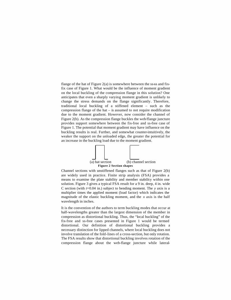
flange of the hat of Figure 2(a) is somewhere between the ss-ss and fix-fix case of Figure 1. What would be the influence of moment gradient on the local buckling of the compression flange in this solution? One anticipates that even a sharply varying moment gradient is unlikely to change the stress demands on the flange significantly. Therefore, traditional local buckling of a stiffened element – such as the compression flange of the hat – is assumed to not require modification due to the moment gradient. However, now consider the channel of Figure 2(b). As the compression flange buckles the web/flange juncture provides support somewhere between the fix-free and ss-free case of Figure 1. The potential that moment gradient may have influence on the buckling results is real. Further, and somewhat counter-intuitively, the weaker the support on the unloaded edge, the greater the potential for an increase in the buckling load due to the moment gradient.

(a) hat section (b) channel section

Figure 2 Section shapes

Channel sections with unstiffened flanges such as that of Figure 2(b) are widely used in practice. Finite strip analysis (FSA) provides a means to examine the plate stability and member stability within one solution. Figure 3 gives a typical FSA result for a 9 in. deep, 4 in. wide C section (with t=0.04 in.) subject to bending moment. The y axis is a multiplier times the applied moment (load factor) which indicates the magnitude of the elastic buckling moment, and the x axis is the half wavelength in inches.

It is the convention of the authors to term buckling modes that occur at half-wavelengths greater than the largest dimension of the member in compression as distortional buckling. Thus, the “local buckling” of the fix-free and ss-free cases presented in Figure 1 would be termed distortional. Our definition of distortional buckling provides a necessary distinction for lipped channels, where local buckling does not involve translation of the fold-lines of a cross-section, but only rotation. The FSA results show that distortional buckling involves rotation of the compression flange about the web-flange juncture while lateral-

torsional buckling involves translation and rotation of the entire section, without any distortion of the cross-section itself. Distortional buckling occurs at about a 10 in. half wavelength, which is relatively long compared to the flange width. Therefore, the influence of moment gradient on the buckling of this section may be of practical interest.

Distortional Lateral -torsional

Figure 3 Finite strip result of the buckling of C section in bending

Analytic Solution: Energy Method

To investigate the influence of stress gradient on plate stability we will consider the buckling of stiffened (Figure 4) and unstiffened (Figure 5) elements via the Rayleigh-Ritz method. As shown in Figures 4 and 5, we consider unequal stresses applied at the ends to account for the influence of moment gradient on the applied stress for a plate isolated from the member.

o

o

Y

min σ max

σ

τ

a

b simply supported

X

τ

τ τ

Figure 4 Stiffened element subject to a stress gradient

o

o

Y

min σ maxσ

τ

a

b

free edge

elastic restrained edge τ τ

X

Figure 5 Unstiffened element subject to a stress gradient

The Rayleigh-Ritz method has been widely applied to determine the buckling stress of plates. In this method, an assumed deflection function satisfying the boundary conditions is used in the expression for the total potential energy Π. The total potential energy is the summation of internal strain energy U of the plate during bending, and the work done by the external forces T. Classical solutions from thin plate theory (e.g. Timoshenko and Gere 1961) result in:

TU +=Π (1)

dxdyyxw

y

w

x

w

y

w

x

wDU

b a

∫ ∫

∂∂∂

−∂

∂

∂

∂−−

∂

∂+

∂

∂=

0 0

22

2

2

2

22

2

2

2

2)1(2

2µ (2)

∫ ∫

∂∂

∂∂+

∂∂+

∂∂−=

b a

xyyx dxdyyw

xw

yw

xwtT

0 0

22

22

τσσ (3)

Using the principle of minimum total potential energy, the equilibrium configuration of the plate is identified by Equations (4).

( )Niwi

K2,10 ==∂

Π∂ (4)

Equation (4) represents a system of N simultaneous homogeneous equations with wi and load s (s max is used in present paper) as unknowns. For nontrivial solution of wi’s, the determinant of the coefficient matrix of the system of equations must vanish. The lowest value of smax that leaves the determinant of the coefficient matrix to be zero is the critical load of the plate.

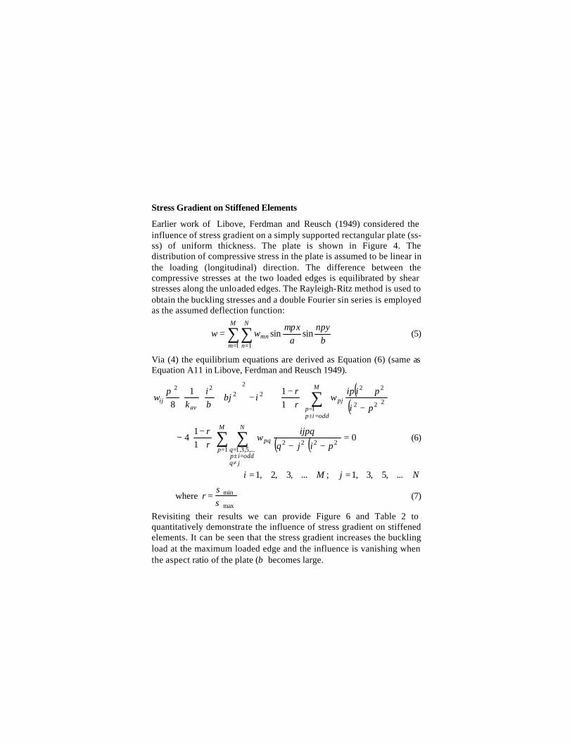
Stress Gradient on Stiffened Elements

Earlier work of Libove, Ferdman and Reusch (1949) considered the influence of stress gradient on a simply supported rectangular plate (ss-ss) of uniform thickness. The plate is shown in Figure 4. The distribution of compressive stress in the plate is assumed to be linear in the loading (longitudinal) direction. The difference between the compressive stresses at the two loaded edges is equilibrated by shear stresses along the unloaded edges. The Rayleigh-Ritz method is used to obtain the buckling stresses and a double Fourier sin series is employed as the assumed deflection function:

∑∑= =

=M

m

N

nmn b

yna

xmww

1 1

sinsinππ

(5)

Via (4) the equilibrium equations are derived as Equation (6) (same as Equation A11 in Libove, Ferdman and Reusch 1949).

( )( )∑

=±= −

+

+−

+

−

+

M

oddipp

pjav

ijpi

piipw

rr

iji

kw

1222

222

22

22

111

8β

βπ

( )( )∑ ∑=

≠=±

=

=−−

+−

−M

p

N

jqoddip

qpq

pijq

ijpqw

rr

1 ,...5,3,12222

011

4 (6)

NjMi ...,5,3,1;...,3,2,1 ==

where max

min

σσ

=r (7)

Revisiting their results we can provide Figure 6 and Table 2 to quantitatively demonstrate the influence of stress gradient on stiffened elements. It can be seen that the stress gradient increases the buckling load at the maximum loaded edge and the influence is vanishing when the aspect ratio of the plate (β) becomes large.

ss

ss

ss

ss

ss

ss

maxσ

maxσ σ

maxσ

tbD

kcr 2

2

maxmax )(π

σ =

σ

Figure 6 kmax vs. plate aspect ratio (ß) for stiffened element

Consistent with our intuition from Figure 1, we can conclude that the influence of stress gradient diminishes quickly for local buckling of a stiffened element, but perhaps not as quickly as is generally assumed in design. The kmax values of Table 1 may be used to predict the increased local buckling stress due to the influence of a stress gradient, and for continuous beams where sharp moment gradients are more likely to persist, the boost may be significant. We now turn to the more complicated and interesting problem of the stability of unstiffened elements under a stress gradient.

Table 1 Numerical results of kmax values for ss-ss stiffened elements r β

-1 -0.8 -0.6 -0.4 -0.2 0 0.2 0.4 0.6 0.8 1

1.0 18.01815.06612.58210.528 8.863 7.533 6.480 5.645 4.979 4.441 4.000 1.2 14.72112.75011.063 9.628 8.410 7.375 6.497 5.751 5.119 4.585 4.134 1.4 12.51911.103 9.877 8.818 7.905 7.117 6.436 5.846 5.333 4.884 4.470 1.6 10.963 9.884 8.935 8.100 7.364 6.712 6.128 5.597 5.105 4.640 4.202 1.8 9.833 8.975 8.210 7.525 6.910 6.353 5.841 5.363 4.907 4.465 4.045 2.0 8.993 8.291 7.656 7.082 6.558 6.079 5.635 5.215 4.810 4.405 4.000 2.5 7.655 7.187 6.754 6.355 5.984 5.638 5.314 5.009 4.718 4.437 4.134 3.0 6.893 6.549 6.227 5.924 5.639 5.368 5.109 4.858 4.608 4.341 4.000 3.5 6.409 6.139 5.882 5.639 5.406 5.182 4.965 4.752 4.540 4.321 4.072 4.0 6.073 5.851 5.639 5.434 5.237 5.045 4.858 4.673 4.486 4.284 4.000 4.5 5.827 5.639 5.456 5.280 5.109 4.941 4.776 4.611 4.443 4.264 4.045 5.0 5.638 5.474 5.315 5.160 5.008 4.858 4.710 4.561 4.408 4.243 4.000 5.5 5.489 5.344 5.202 5.063 4.926 4.791 4.656 4.520 4.380 4.227 4.030 6.0 5.367 5.237 5.109 4.983 4.858 4.735 4.611 4.486 4.355 4.213 4.000 6.5 5.267 5.148 5.031 4.915 4.801 4.687 4.573 4.456 4.335 4.201 4.022 7.0 5.181 5.072 4.965 4.858 4.752 4.646 4.540 4.431 4.317 4.191 4.000 7.5 5.108 5.007 4.908 4.809 4.710 4.611 4.511 4.408 4.301 4.182 4.017 8.0 5.045 4.951 4.858 4.765 4.673 4.580 4.486 4.389 4.287 4.174 4.000 8.5 4.990 4.902 4.814 4.727 4.640 4.552 4.463 4.371 4.274 4.166 4.013 9.0 4.941 4.858 4.776 4.694 4.611 4.528 4.443 4.355 4.263 4.160 4.000 9.5 4.898 4.820 4.742 4.663 4.585 4.506 4.425 4.341 4.253 4.154 4.011

10.0 4.860 4.785 4.711 4.636 4.561 4.486 4.408 4.328 4.243 4.148 4.000 11.0 4.791 4.723 4.656 4.588 4.520 4.451 4.380 4.306 4.227 4.139 4.000 12.0 4.735 4.673 4.611 4.549 4.486 4.421 4.355 4.287 4.213 4.130 4.000 13.0 4.687 4.630 4.573 4.515 4.456 4.396 4.335 4.270 4.201 4.123 4.000 14.0 4.646 4.593 4.540 4.486 4.431 4.375 4.317 4.256 4.191 4.117 4.000 15.0 4.611 4.561 4.511 4.460 4.408 4.355 4.301 4.243 4.182 4.112 4.000 16.0 4.580 4.533 4.486 4.438 4.389 4.339 4.287 4.232 4.174 4.107 4.000 17.0 4.552 4.508 4.463 4.418 4.371 4.324 4.274 4.222 4.166 4.102 4.000 18.0 4.528 4.486 4.443 4.400 4.355 4.310 4.263 4.213 4.160 4.098 4.000 19.0 4.506 4.465 4.425 4.383 4.341 4.298 4.253 4.205 4.154 4.095 4.000 20.0 4.486 4.447 4.408 4.369 4.328 4.287 4.243 4.198 4.148 4.091 4.000 21.0 4.467 4.431 4.393 4.355 4.317 4.277 4.235 4.191 4.143 4.088 4.000 22.0 4.451 4.415 4.380 4.343 4.306 4.267 4.227 4.185 4.139 4.086 4.000 23.0 4.435 4.402 4.367 4.332 4.296 4.259 4.220 4.179 4.134 4.083 4.000 24.0 4.421 4.389 4.355 4.322 4.287 4.251 4.213 4.174 4.130 4.081 4.000 25.0 4.408 4.377 4.345 4.312 4.278 4.243 4.207 4.169 4.127 4.078 4.000 26.0 4.396 4.366 4.335 4.303 4.270 4.237 4.201 4.164 4.123 4.076 4.000 27.0 4.385 4.355 4.325 4.295 4.263 4.230 4.196 4.160 4.120 4.074 4.000 28.0 4.375 4.346 4.317 4.287 4.256 4.224 4.191 4.156 4.117 4.073 4.000 29.0 4.365 4.337 4.308 4.279 4.250 4.219 4.186 4.152 4.114 4.071 4.000 30.0 4.355 4.328 4.301 4.273 4.243 4.213 4.182 4.148 4.112 4.069 4.000

Stress Gradient on Unstiffened Elements

Double Curvature Bending

MB

MB

MB MA

MA

MA

Single Curvature Bending

Figure 7 Channel subject to moment gradient

Consider a channel under moment gradient as shown in Figure 7. Distortional buckling (“local buckling” of the unstiffened element) of this channel may be considered by isolating the compression flange and modeling the flange as a thin plate supported on one unloaded edge, free on the opposite edge and loaded with unequal axial stresses, as shown in Figure 5. The web’s contribution to the stability of the flange may be treated as a rotational spring along the supported edge. As discussed in Schafer and Peköz (1999) this rotational support is stress dependent and may have a net positive or negative contribution to the stiffness depending on whether the buckling is triggered by buckling of the web first (net negative stiffness) or buckling of the flange (net positive stiffness). Our analysis here will focus on the case where the flange buckles before the web. The specific thin plate model examined is shown in detail in Figure 5. The difference between the compressive stresses is equilibrated by uniform shear stresses acting along the longitudinal supported edge. Shear stresses along the two compressive loaded edges are linearly distributed. Elastic rotational restraint from the web is also applied along the longitudinal supported edge. The strain energy due to the elastic restraint U2 needs to be included in the total potential energy U, resulting in:

TUU ++=Π 21 (8)

where U1 is the strain energy due to the bending of the plate, Equation (2); and

∫

∂∂=

=

a

y

dxywSU

0

2

02 2

(9)

The uniform shear stress at the edge y=0 can be determined by force equilibrium in the x direction, Equation (9) is the result. In addition, along the free edge no stress exists, Equation (10).

ab

yxy)( minmax

0|σσ

τ−

== (10)

0| ==byxyτ (11)

Equilibrium is enforced by insuring ∑ = 0xF , ∑ = 0yF ,

∑ = 00M (about the origin). The internal shear stress distribution is

assumed to be linear along the plate width and uniform in the x direction:

−

−=

by

arb

xy 1)1(

maxστ (12)

Assuming plane stress conditions, then equilibrium can be found:

0=∂

∂+

∂∂

yxxyx τσ

(13)

0=∂

∂+

∂

∂

xyxyy τσ

(14)

where the body force has been neglected. By substituting Equation (11) into Equations (12) and (13) along with the fact that

maxmin0| σσσ rxx === , the compressive stresses can be obtained in

functional form as:

+

−= r

axr

x)1(

maxσσ (15)

0=yσ (16)

Deflection function and boundary conditions

The Rayleigh-Ritz method is an approximate approach and the accuracy of the results depends on how closely the assumed deflection function w(x,y) describes the true deflection. In general, the selected deflection function should satisfy the boundary conditions of the plate. For the model of Figure 5, a total of six boundary conditions are observed and stated below.

Simply supported at the transverse, loaded edges:

0)( 0 ==xw (17)

0)( ==axw (18)

Elastic restraint against rotation along one supported longitudinal edge:

0)( 0 ==yw (19)

002

2

2

2

==

∂∂

=

∂∂

+∂∂

yyyw

Sx

wy

wD µ (20)

One free longitudinal edge:

02

2

2

2

=

∂

∂+

∂

∂

=byx

w

y

wD µ (21)

0)2( 2

3

3

3

=

∂∂∂

−+∂∂

=byyx

wyw

D µ (22)

Due to the complicated boundary conditions, a single trigonometric (sin or cos) term is not appropriate to approximate the real deflection in either direction. However, the linearity of differential equations (19) to (22) imply that the deflection function ),( yxw can be formed as

∑=

N

iii xByA

1

)()( , where iA is a function of y alone and iB is a

function of x alone. If, for every i, Ai(y)Bi(x) is compatible with all the boundary conditions, then the linear summation of each term Ai(y)Bi(x)

will satisfy the boundary conditions. In this paper, three different approximate deflection functions are proposed and examined.

Deflection function 1

The first deflection function considered, Equation (22), is motivated by the work of Lundquist and Stowell (1942) who explored the buckling of unstiffened element subject to uniform compressive stresses. Lundquist and Stowell employed a trigonometric term in the longitudinal direction and a polynomial term in the transverse direction to establish the deflection function, as below:

+

+

+

+=

ax

bya

bya

bya

byB

byAw πsin

2

3

3

2

4

1

5

(23)

where A and B are arbitrary deflection amplitudes and 963.41 −=a ,

852.92 =a , and 778.93 −=a . The deflection curve across the width of the plate is taken as the sum of a straight line and a cantilever-deflection curve. The values of a1, a2 and a3 were determined by taking the proportion of two deflection curves that gave the lowest buckling stress for a fixed-edge flange with µ=0.3.

For the unstiffened element under a stress gradient, the single trigonometric term in the loading direction is no longer appropriate. We therefore use a summation of trigonometric terms in the longitudinal direction and polynomial terms in the transverse direction for the deflection function, Equation (23), where the values of a1, a2 and a3 are same as Equation (22).

+

+

+

+= ∑= a

xibya

bya

bya

byB

byAw

N

i

πsin1

2

3

3

2

4

1

5

(24)

The arbitrary amplitudes A and B are actually related to each other; the relationship can be obtained by substituting Equation (22) into boundary condition (19), resulting in

ADa

SbB

32= (25)

Therefore, the deflection function, Equation (23), may be simplified as:

+

+

+

+= ∑

= axi

bya

bya

bya

by

DaSb

byww

N

ii

πsin21

2

3

3

2

4

1

5

3

(26) The equilibrium equations can be constructed by substituting the deflection function into the total potential energy expression Equations (7) and taking the derivative of the function as Equation (4). The buckling stress smax is the minimum eigenvalue of the resulting matrix of equilibrium expressions. The size of matrix is .NN ×

It should be noted that deflection function 1 is not compatible with boundary the conditions, Equations (20) and (21). However, it was found to give reasonable results in the research done by Lundquist and Stowell (1942) and was thus considered here.

Deflection function 2

Unlike deflection function 1 which is based on a physical representation of the expected shape, deflection function 2 is a more general combination of polynomials and trigonometric functions. A fourth order polynomial is assumed for the transverse deflection and a sin function for the longitudinal deflection as given in Equation (26).

( )

+++= ∑

=axi

ycycycycwwN

iiiiii

πsin

1

44

33

221 (27)

The deflection function must satisfy all the boundary conditions. Therefore, the parameters 1ic , 2ic , 3ic , 4ic are determined by

substituting Equation 26 into the boundary conditions of Equations (16) to (21), resulting in:

11 =ic (28)

DS

ci 22 = (29)

−+

−×

−

−−−−+=

22

12

)2()2(2

2

222

1

22

422

321

3212

22

3212

22

321

2

222

321

2

22

3

a

biDk

Sb

a

bi

Dkk

S

DkkkabSi

kkkai

DkkaSbi

kkabici

πµ

πµ

πµπµπµπµ

(30)

DkkS

DkkabSi

kkai

DkkaSbi

kkabici

31322

22

322

22

312

222

312

22

4 )2()2(2

−−−−−+= πµπµπµπµ

(31) Ni K,2,1=

where

2

322

1 6a

bibk πµ−= (32)

2

222

23)2(6

abik πµ−−= (33)

22

322

212

422

1

2

34)2(2412

ka

bik

b

ka

bikbk πµπµ −+−−= (34)

The equilibrium equations can be constructed by the same method as described for deflection function 1, the buckling stress (s max)cr is the minimum eigenvalue of the resulting NN × matrix of equilibrium expressions.

Deflection function 3

As an extension of the second deflection function a third deflection function using a 5th order polynomial in the transverse direction was also considered:

( ) ( )[ ]

++++++=∑

=axi

yqyqyqwypypypypwwN

iiiiiiiiii

πsin

1

53

42

312

44

33

2211

(35)

where 1iw , 2iw are arbitrary deflection amplitudes. The parameters p and q were determined by the boundary conditions.

11 =ip (36)

DS

p i 22 = (37)

12

1422

2

222

112

22

3 22 ka

Mbi

a

biDk

S

ka

bipi

πµ

πµ

πµ +

−+= (38)

14 Mpi = (39)

1

22

12

2422

1

3

12

522

11220

kMb

kaMbi

kb

kabiq i −+−= πµπµ (40)

22 Mqi = (41)

13 =iq (42)

where

2

322

1 6a

bibk πµ−= (43)

2

222

23)2(6

abik πµ−−= (44)

22

322

1

22

422

31

244

)2(1

12k

ba

biv

kb

a

bik

−−−

−=

ππµ (45)

3131

222

312

22

32

22

322

22

1 2)2()2(

kDkS

DkkSbi

kkabi

DkkbSi

kkaiM +−−−+−= πµπµπµπµ

(46)

31

3

312

522

32

2

322

422

220605)2(

kkb

kkabi

kkb

kkabiM +−−−= πµπµ (47)

The size of the resulting matrix of equilibrium expressions is NN 22 × .

Verification of three deflection functions

Finite element analysis using ABAQUS 6.2 was employed to examine the results of the previous Rayleigh-Ritz solutions. The S4R5 shell element was used for the thin plate with E=29500 ksi and µ=0.3. The element size is 0.1 in. x 0.1 in. The plate is simply supported along three edges , and free along one unloaded edge. The uneven load is equilibrated by shear forces acting along one simply supported edge, similar to Figure 5.

Figure 8 shows the buckled shape for the case with r=0, a=10 in., b=3 in., t=0.0333 in., and S=0 kips-in/in. Table 2 provides the comparison of the analytical solutions (DF1, DF2, DF3) with ABAQUS results (FEM). In general, all three deflection functions give good agreement with the finite element results. Deflection functions 2 and 3 have closer results to the FEM, with average error less than 1%. Deflection function 1 provides systematically higher buckling stress than the FEM results and the other two functions, and the error grows when the stress gradient effect is large or S is large. Since deflection function 2 provides both accuracy and reasonable computational efficiency, it is selected for further analyses. According to a convergence study of deflection function 2, the number of terms to be kept in the expansions (and thus the size of the NxN matrix to be solved,) is selected via the following rules.

a/b<=10, N=20; a/b>10 and a/b<=20, N=40; a/b>20 and a/b<=40, N=60; a/b>40 and a/b<=60, N=80.

(a) ABAQUS result (b) Analytical solution

Figure 8 Buckling shapes of unstiffened element for stress gradient factor r = 0

Table 2 Results of numerical models with different deflection functions r a

(in.) b

(in.) t

(in.) S

(kip-in/in) DF1/FEM DF2/FEM DF3/FEM

1 10 2.5 0.04 0 1.0011 0.9990 0.9979 0.9 10 2.5 0.04 0 1.0011 0.9989 0.9979 0.7 10 2.5 0.04 0 1.0015 0.9988 0.9977 0.5 10 2.5 0.04 0 1.0023 0.9985 0.9973 0.3 10 2.5 0.04 0 1.0035 0.9981 0.9968 0.1 10 2.5 0.04 0 1.0050 0.9976 0.9962 0 10 2.5 0.04 0 1.0058 0.9973 0.9959

-0.1 10 2.5 0.04 0 1.0066 0.9971 0.9957 -0.3 10 2.5 0.04 0 1.0085 0.9968 0.9951 -0.5 10 2.5 0.04 0 1.0107 0.9965 0.9947 -0.7 10 2.5 0.04 0 1.0132 0.9963 0.9943 -0.9 10 2.5 0.04 0 1.0160 0.9963 0.9940

Case 1

-1 10 2.5 0.04 0 1.0196 0.9964 0.9936 1 10 2 0.05 0 1.0034 1.0019 1.0009

0.9 10 2 0.05 0 1.0035 1.0019 1.0009 0.7 10 2 0.05 0 1.0038 1.0016 1.0006 0.5 10 2 0.05 0 1.0044 1.0011 1.0000 0.3 10 2 0.05 0 1.0052 1.0006 0.9993 0.1 10 2 0.05 0 1.0060 0.9999 0.9985 0 10 2 0.05 0 1.0065 0.9996 0.9982

-0.1 10 2 0.05 0 1.0069 0.9992 0.9978 -0.3 10 2 0.05 0 1.0081 0.9987 0.9971 -0.5 10 2 0.05 0 1.0093 0.9982 0.9964 -0.7 10 2 0.05 0 1.0108 0.9978 0.9959 -0.9 10 2 0.05 0 1.0125 0.9974 0.9953

Case 2

-1 10 2 0.05 0 1.0133 0.9972 0.9950 1 10 3 0.0333 0 1.0004 0.9979 0.9968

0.9 10 3 0.0333 0 1.0005 0.9978 0.9967 0.7 10 3 0.0333 0 1.0009 0.9978 0.9966 0.5 10 3 0.0333 0 1.0019 0.9977 0.9965 0.3 10 3 0.0333 0 1.0035 0.9974 0.9962 0.1 10 3 0.0333 0 1.0056 0.9972 0.9958 0 10 3 0.0333 0 1.0068 0.9971 0.9957

-0.1 10 3 0.0333 0 1.0081 0.9970 0.9955 -0.3 10 3 0.0333 0 1.0110 0.9969 0.9952 -0.5 10 3 0.0333 0 1.0143 0.9970 0.9951 -0.7 10 3 0.0333 0 1.0181 0.9974 0.9952 -0.9 10 3 0.0333 0 1.0224 0.9979 0.9954

Case 3

-1 10 3 0.0333 0 0.9931 0.9983 0.9955 1 10 3 0.0333 inf 0.9981 0.9979 0.9975

0.9 10 3 0.0333 inf 0.9991 0.9978 0.9974 0.7 10 3 0.0333 inf 1.0073 0.9969 0.9964 0.5 10 3 0.0333 inf 1.0205 0.9956 0.9951 0.3 10 3 0.0333 inf 1.0363 0.9944 0.9938 0.1 10 3 0.0333 inf 1.0540 0.9933 0.9927 0 10 3 0.0333 inf 1.0636 0.9929 0.9922

-0.1 10 3 0.0333 inf 1.0735 0.9926 0.9918 -0.3 10 3 0.0333 inf 1.0947 0.9920 0.9911 -0.5 10 3 0.0333 inf 1.1176 0.9917 0.9907 -0.7 10 3 0.0333 inf 1.1421 0.9917 0.9905 -0.9 10 3 0.0333 inf 1.1684 0.9918 0.9904

Case 4

-1 10 3 0.0333 inf 1.1822 0.9920 0.9905 Average 1.0237 0.9971 0.9958

Standard deviation 0.0427 0.0026 0.0026

Table 3 Numerical results of kmax values of ss-free unstiffened element r β

-1 -0.8 -0.6 -0.4 -0.2 0 0.2 0.4 0.6 0.8 1

1.0 4.765 4.298 3.841 3.402 2.992 2.621 2.299 2.025 1.796 1.606 1.447 1.2 3.605 3.263 2.930 2.609 2.306 2.029 1.785 1.576 1.399 1.252 1.128 1.4 2.894 2.631 2.375 2.127 1.891 1.673 1.477 1.307 1.163 1.041 0.938 1.6 2.423 2.214 2.009 1.810 1.619 1.440 1.278 1.134 1.010 0.905 0.816 1.8 2.093 1.921 1.752 1.588 1.430 1.279 1.140 1.016 0.906 0.813 0.733 2.0 1.852 1.707 1.565 1.426 1.291 1.162 1.041 0.930 0.832 0.747 0.674 2.5 1.465 1.363 1.264 1.166 1.070 0.976 0.885 0.798 0.718 0.647 0.584 3.0 1.241 1.164 1.088 1.013 0.939 0.866 0.794 0.723 0.655 0.592 0.535 3.5 1.096 1.035 0.974 0.914 0.854 0.795 0.735 0.676 0.616 0.559 0.506 4.0 0.996 0.945 0.894 0.844 0.794 0.744 0.694 0.642 0.590 0.538 0.487 4.5 0.922 0.879 0.836 0.793 0.750 0.707 0.663 0.618 0.571 0.523 0.474 5.0 0.866 0.828 0.791 0.753 0.715 0.677 0.639 0.599 0.556 0.512 0.465 5.5 0.822 0.789 0.755 0.722 0.688 0.654 0.619 0.583 0.545 0.503 0.458 6.0 0.786 0.756 0.726 0.696 0.666 0.635 0.603 0.571 0.536 0.497 0.453 6.5 0.757 0.730 0.703 0.675 0.647 0.619 0.590 0.560 0.528 0.491 0.449 7.0 0.733 0.708 0.683 0.657 0.632 0.606 0.579 0.551 0.521 0.487 0.446 7.5 0.712 0.689 0.665 0.642 0.618 0.594 0.569 0.543 0.515 0.483 0.443 8.0 0.694 0.672 0.651 0.629 0.607 0.584 0.561 0.537 0.510 0.480 0.441 8.5 0.678 0.658 0.638 0.617 0.597 0.576 0.554 0.531 0.506 0.477 0.439 9.0 0.664 0.645 0.627 0.607 0.588 0.568 0.547 0.525 0.502 0.474 0.438 9.5 0.652 0.634 0.617 0.598 0.580 0.561 0.541 0.521 0.498 0.472 0.436

10.0 0.641 0.624 0.608 0.590 0.573 0.555 0.536 0.516 0.495 0.470 0.435 11.0 0.623 0.607 0.592 0.577 0.561 0.544 0.527 0.509 0.489 0.467 0.434 12.0 0.607 0.593 0.579 0.565 0.551 0.535 0.520 0.503 0.485 0.464 0.432 13.0 0.594 0.582 0.569 0.556 0.542 0.528 0.513 0.498 0.481 0.461 0.431 14.0 0.583 0.572 0.560 0.547 0.535 0.522 0.508 0.494 0.478 0.459 0.431 15.0 0.574 0.563 0.552 0.540 0.528 0.516 0.503 0.490 0.475 0.457 0.430 16.0 0.566 0.555 0.545 0.534 0.523 0.511 0.499 0.486 0.472 0.456 0.429 17.0 0.558 0.549 0.539 0.528 0.518 0.507 0.496 0.483 0.470 0.454 0.429 18.0 0.552 0.543 0.533 0.524 0.514 0.503 0.492 0.481 0.468 0.453 0.429 19.0 0.546 0.537 0.528 0.519 0.510 0.500 0.489 0.478 0.466 0.452 0.428 20.0 0.541 0.533 0.524 0.515 0.506 0.497 0.487 0.476 0.464 0.451 0.428 21.0 0.536 0.528 0.520 0.512 0.503 0.494 0.484 0.474 0.463 0.450 0.428 22.0 0.532 0.524 0.516 0.508 0.500 0.491 0.482 0.472 0.461 0.449 0.428 23.0 0.528 0.521 0.513 0.505 0.497 0.489 0.480 0.471 0.460 0.448 0.427 24.0 0.524 0.517 0.510 0.503 0.495 0.487 0.478 0.469 0.459 0.447 0.427 25.0 0.521 0.514 0.507 0.500 0.493 0.485 0.477 0.468 0.458 0.446 0.427 26.0 0.518 0.511 0.505 0.498 0.490 0.483 0.475 0.466 0.457 0.446 0.427 27.0 0.515 0.509 0.502 0.496 0.489 0.481 0.474 0.465 0.456 0.445 0.427 28.0 0.513 0.506 0.500 0.493 0.487 0.480 0.472 0.464 0.455 0.445 0.427 29.0 0.510 0.504 0.498 0.492 0.485 0.478 0.471 0.463 0.454 0.444 0.427 30.0 0.508 0.502 0.496 0.490 0.483 0.477 0.470 0.462 0.454 0.444 0.427

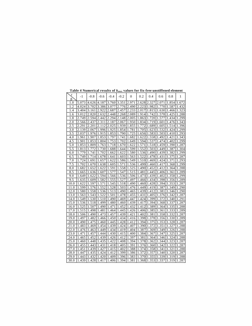
Table 4 Numerical results of kmax values for fix-free unstiffened element r β

-1 -0.8 -0.6 -0.4 -0.2 0 0.2 0.4 0.6 0.8 1

1.0 5.073 4.626 4.187 3.760 3.351 2.971 2.628 2.327 2.071 1.854 1.672 1.2 4.024 3.702 3.386 3.077 2.776 2.490 2.223 1.982 1.770 1.587 1.432 1.4 3.404 3.161 2.922 2.687 2.457 2.233 2.017 1.815 1.630 1.466 1.323 1.6 3.012 2.820 2.632 2.448 2.268 2.089 1.914 1.742 1.578 1.425 1.288 1.8 2.749 2.594 2.442 2.294 2.148 2.005 1.863 1.720 1.577 1.434 1.299 2.0 2.566 2.437 2.311 2.187 2.067 1.950 1.834 1.719 1.601 1.476 1.343 2.5 2.291 2.201 2.112 2.025 1.939 1.855 1.772 1.689 1.605 1.514 1.396 3.0 2.139 2.067 1.996 1.925 1.854 1.781 1.705 1.623 1.532 1.424 1.299 3.5 2.037 1.976 1.915 1.853 1.790 1.725 1.656 1.583 1.503 1.410 1.293 4.0 1.961 1.907 1.853 1.797 1.741 1.682 1.622 1.558 1.492 1.421 1.343 4.5 1.901 1.853 1.804 1.753 1.702 1.649 1.594 1.537 1.474 1.402 1.299 5.0 1.853 1.809 1.763 1.718 1.670 1.622 1.571 1.518 1.459 1.390 1.287 5.5 1.813 1.772 1.730 1.688 1.644 1.599 1.552 1.503 1.449 1.387 1.304 6.0 1.779 1.741 1.702 1.662 1.622 1.580 1.536 1.490 1.439 1.382 1.299 6.5 1.749 1.714 1.678 1.641 1.603 1.563 1.522 1.478 1.431 1.375 1.287 7.0 1.724 1.691 1.657 1.622 1.586 1.549 1.510 1.469 1.424 1.371 1.293 7.5 1.702 1.670 1.638 1.605 1.571 1.536 1.499 1.460 1.417 1.368 1.299 8.0 1.682 1.652 1.622 1.591 1.558 1.525 1.490 1.452 1.412 1.364 1.288 8.5 1.665 1.636 1.607 1.577 1.547 1.515 1.481 1.445 1.406 1.361 1.289 9.0 1.649 1.622 1.594 1.566 1.536 1.506 1.473 1.439 1.402 1.358 1.299 9.5 1.635 1.609 1.582 1.555 1.527 1.497 1.466 1.434 1.398 1.356 1.289

10.0 1.622 1.597 1.571 1.545 1.518 1.490 1.460 1.428 1.394 1.353 1.287 11.0 1.599 1.576 1.552 1.528 1.503 1.476 1.449 1.419 1.387 1.349 1.290 12.0 1.580 1.558 1.536 1.513 1.490 1.465 1.439 1.412 1.381 1.346 1.290 13.0 1.563 1.543 1.522 1.501 1.478 1.455 1.431 1.405 1.376 1.342 1.287 14.0 1.549 1.530 1.510 1.490 1.469 1.447 1.424 1.399 1.372 1.340 1.291 15.0 1.536 1.518 1.499 1.480 1.460 1.439 1.417 1.394 1.368 1.337 1.287 16.0 1.525 1.507 1.490 1.471 1.452 1.432 1.412 1.389 1.364 1.335 1.288 17.0 1.515 1.498 1.481 1.464 1.445 1.426 1.406 1.385 1.361 1.333 1.289 18.0 1.506 1.490 1.473 1.457 1.439 1.421 1.402 1.381 1.358 1.332 1.287 19.0 1.497 1.482 1.466 1.450 1.434 1.416 1.398 1.378 1.356 1.330 1.289 20.0 1.490 1.475 1.460 1.445 1.428 1.412 1.394 1.375 1.353 1.328 1.287 21.0 1.483 1.469 1.454 1.439 1.424 1.407 1.390 1.372 1.351 1.327 1.288 22.0 1.476 1.463 1.449 1.434 1.419 1.404 1.387 1.369 1.349 1.326 1.288 23.0 1.471 1.457 1.444 1.430 1.415 1.400 1.384 1.367 1.347 1.325 1.287 24.0 1.465 1.452 1.439 1.426 1.412 1.397 1.381 1.364 1.346 1.324 1.288 25.0 1.460 1.448 1.435 1.422 1.408 1.394 1.378 1.362 1.344 1.323 1.287 26.0 1.455 1.443 1.431 1.418 1.405 1.391 1.376 1.360 1.342 1.322 1.287 27.0 1.451 1.439 1.427 1.415 1.402 1.388 1.374 1.358 1.341 1.321 1.288 28.0 1.447 1.435 1.424 1.412 1.399 1.386 1.372 1.357 1.340 1.320 1.287 29.0 1.443 1.432 1.420 1.409 1.396 1.383 1.370 1.355 1.339 1.319 1.288 30.0 1.439 1.428 1.417 1.406 1.394 1.381 1.368 1.353 1.337 1.319 1.287

Results

Two unstiffened elements are investigated here, one where the supported longitudinal edge has no rotational restraint (ss-free) and one where the supported has infinite rotational restraint (fix-free). The plate buckling coefficient kmax for the elements subject to a variety of stress gradients is summarized in Table 3 for the ss-free case and Table 4 for the fix-free case. Figure 9 and Figure 10 give a graphic representation of the stress gradient effect on these two different unstiffened elements. For the ss-free unstiffened plate under uniform compression, the plate buckling coefficient k asymptotes to 0.425. It is shown in Figure 9 that the stress gradient boosts the buckling stress at the maximum loaded edge greatly, especially when the plate aspect ratio (β) is less than 10. Similar results are observed for the fix-free unstiffened element in Figure 10, the buckling coefficient kmax converges to 1.287 (buckling coefficient for uniform compression) gradually.

ss

free

ss

free

ss

free

max

max

maxσ

tbD

kcr 2

2

maxmax )(π

σ =

Figure 9 kmax vs. plate aspect ratio (ß) for ss-free unstiffened element

Figure 11 shows the relation between the plate buckling coefficient kmax and the stress gradient factor r for a ss-free unstiffened element.

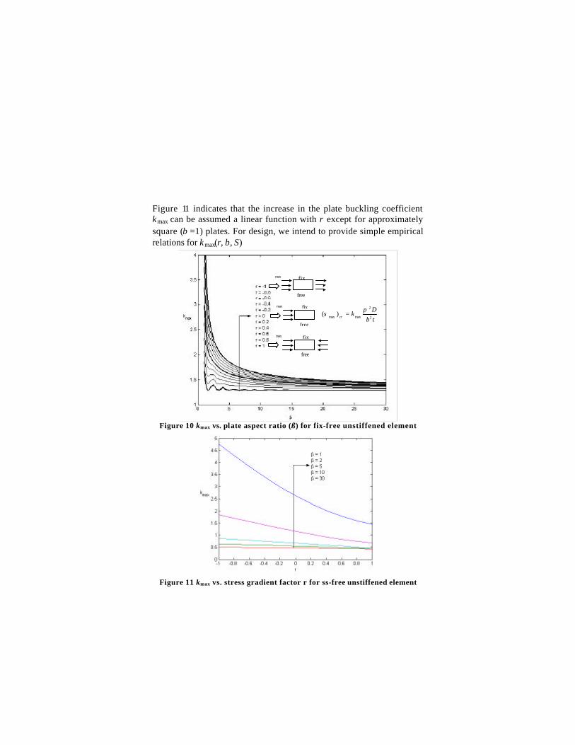
Figure 11 indicates that the increase in the plate buckling coefficient kmax can be assumed a linear function with r except for approximately square (β =1) plates. For design, we intend to provide simple empirical relations for kmax(r, β, S)

fix

free

fix

free

fix

free

max

max

max

tbD

kcr 2

2

maxmax )(π

σ =

Figure 10 kmax vs. plate aspect ratio (ß) for fix-free unstiffened element

Figure 11 kmax vs. stress gradient factor r for ss-free unstiffened element

Discussion

σmax

Figure 12 Comparison of the stress gradient effects (r=0)

Figure 12 shows a comparison of the three different elements subject to a stress gradient with r=0 (compressive stress only acting on one edge). The y axis is the stress gradient solutions derived here, normalized to k0 which is the solution for elements under uniform stress (no stress gradient, r=1). As shown in Figure 12, the stress gradient has the most influence on the ss-free unstiffened element. The plate buckling coefficient for the stiffened element kmax converges rapidly to approximately 1.1k0 and then more slowly to 1.0 k0. For the ss-free unstiffened element kmax>1.1k0, even for ß as large as 30. However, the fix-free unstiffened element is approximately the same as the stiffened element. The moment gradient influence on unstiffened sections (Figure 2b) can be expected to fall in the area between the curves of ss-free and fix-free unstiffened elements of Figure 12. If we compare to the section in Figure 3, if a moment gradient went from a maximum to an inflection point (M=0, r=0) over a length of 4 in. x 30 = 120 in. (10 ft.) then one would expect a boost in the plate buckling coefficient of as much as 1.1 – if the moment gradient is sharper the boost would be greater. The significant influence on the unstiffened element, particularly in the case where the web provides little restraint, can make the moment gradient a considerable factor when one analyzes the buckling strength. These solutions suggest a reserve that may be relied

upon in many loading cases, particularly with regard to unstiffened elements.

Conclusions

An analytical method to determine the buckling stress of thin plates subject to a stress gradient is derived and verified by finite element analysis. The results show that under a stress gradient, the buckling stress at the maximum loaded end is higher than for the same plate under uniform compressive stresses. The influence of stress gradient on both stiffened and unstiffened elements was derived and quantified. Compared with the stiffened element, the unstiffened element exhibits a stronger dependency on the applied stress gradient and the dependency decreases more slowly as the plate aspect ratio becomes large (the plate becomes longer). Ignoring the moment gradient effect on plate stability leads to conservative predictions of the strength of thin-walled beams, particularly for members with unstiffened flanges where the web provides little restraint to the flange. The authors intend to seek simple empirical expression kmax(r, β, S) for thin plates and help to further develop specification provisions that may include the moment gradient effect on plate stability of thin-walled beams.

Acknowledgement

The sponsorship of the American Iron and Steel Institute is gratefully acknowledged.

Appendix. - References ABAUQS (2001). ABAQUS Version 6.2, ABAQUS, Inc. Pawtucket,

RI. (www.abaqus.com) Lau, S.C.W., Hancock, G.J. (1987). “Distortional Buckling Formulas

for Channel Columns” ASCE, Journal of Structural Engineering. 113 (5) 1063-1078.

Lundquist E., Stowell E. (1942). “Critical Compressive Stress for Outstanding Flanges”. NACA Report No. 734. National Advisory Committee for Aeronautics, Washington, 1942.

Libove, C., Ferdman, S., Reusch, J. (1949). “Elastic Buckling of A Simply Supported Plate Under A Compressive Stress That Varies Linearly in the Direction of Loading”. NACA Technical Notet No.

1891. National Advisory Committee for Aeronautics, Washington, 1949.

Schafer, B.W., Peköz, T. (1999). “Laterally Braced Cold-Formed Steel Flexural Members with Edge Stiffened Flanges” ASCE, Journal of Structural Engineering. 125 (2) 118-127.

Timoshenko, S.P., Gere, J.M. (1961). “Theory of Elastic Stability”, Second Edition. McGrqw-Hill Book Co., 1961

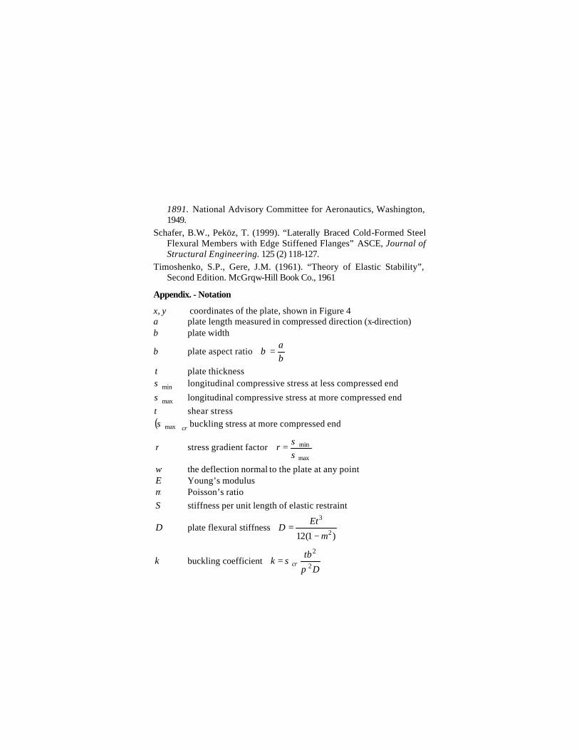
Appendix. - Notation

x, y coordinates of the plate, shown in Figure 4 a plate length measured in compressed direction (x-direction) b plate width

β plate aspect ratio

=

ba

β

t plate thickness

minσ longitudinal compressive stress at less compressed end

maxσ longitudinal compressive stress at more compressed end τ shear stress ( )crmaxσ buckling stress at more compressed end

r stress gradient factor

=

max

min

σσr

w the deflection normal to the plate at any point E Young’s modulus µ Poisson’s ratio S stiffness per unit length of elastic restraint

D plate flexural stiffness

−=

)1(12 2

3

µ

EtD

k buckling coefficient

=

D

tbk cr 2

2

πσ

maxk buckling coefficient at maximum loaded edge

( )D

tbk cr 2

2

maxmaxπ

σ=

avk average buckling coefficient ( )D

tbrk crav 2

2

max 21

πσ

+=