Article

Stress-Function Variational Method for Accurate Free-EdgeInterfacial Stress Analysis of Adhesively Bonded Single-LapJoints and Single-Sided Joints

Xiang-Fa Wu *, Youhao Zhao and Oksana Zholobko

�����������������

Citation: Wu, X.-F.; Zhao, Y.;

Zholobko, O. Stress-Function

Variational Method for Accurate

Free-Edge Interfacial Stress Analysis

of Adhesively Bonded Single-Lap

Joints and Single-Sided Joints. J.

Compos. Sci. 2021, 5, 197. https://

doi.org/10.3390/jcs5080197

Academic Editor:

Francesco Tornabene

Received: 18 June 2021

Accepted: 20 July 2021

Published: 23 July 2021

Publisher’s Note: MDPI stays neutral

with regard to jurisdictional claims in

published maps and institutional affil-

iations.

Copyright: © 2021 by the authors.

Licensee MDPI, Basel, Switzerland.

This article is an open access article

distributed under the terms and

conditions of the Creative Commons

Attribution (CC BY) license (https://

creativecommons.org/licenses/by/

4.0/).

Department of Mechanical Engineering, North Dakota State University, Fargo, ND 58108, USA;youhao.zhao@ndsu.edu (Y.Z.); Oksana.Zholobko@ndsu.edu (O.Z.)* Correspondence: xiangfa.wu@ndsu.edu; Fax: +1-701-231-8913

Abstract: Large free-edge interfacial stresses induced in adhesively bonded joints (ABJs) are respon-sible for the commonly observed debonding failure in ABJs. Accurate and efficient stress analysisof ABJs is important to the design, structural optimization, and failure analysis of ABJs subjectedto external mechanical and thermomechanical loads. This paper generalizes the high-efficiencysemi-analytic stress-function variational methods developed by the authors for accurate free-edgeinterfacial stress analysis of ABJs of various geometrical configurations. Numerical results of theinterfacial stresses of two types of common ABJs, i.e., adhesively bonded single-lap joints and adhe-sively single-sided joints, are demonstrated by using the present method, which are further validatedby finite element analysis (FEA). The numerical procedure formulated in this study indicates thatthe present semi-analytic stress-function variational method can be conveniently implemented foraccurate free-edge interfacial stress analysis of various type of ABJs by only slightly modifying theforce boundary conditions. This method is applicable for strength analysis and structural design ofbroad ABJs made of multi-materials such as composite laminates, smart materials, etc.

Keywords: adhesively bonded joint (ABJ); free-edge stresses; stress-function variational method;debonding; interfacial stress; elasticity

1. Introduction

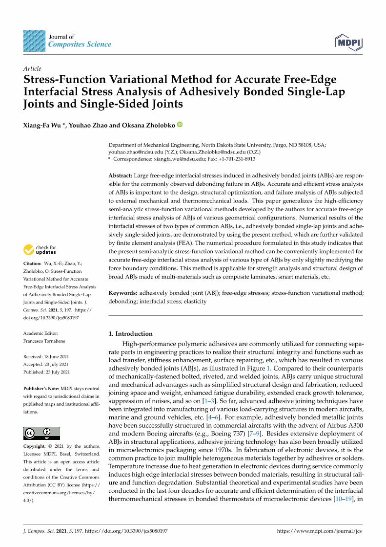
High-performance polymeric adhesives are commonly utilized for connecting sepa-rate parts in engineering practices to realize their structural integrity and functions such asload transfer, stiffness enhancement, surface repairing, etc., which has resulted in variousadhesively bonded joints (ABJs), as illustrated in Figure 1. Compared to their counterpartsof mechanically-fastened bolted, riveted, and welded joints, ABJs carry unique structuraland mechanical advantages such as simplified structural design and fabrication, reducedjoining space and weight, enhanced fatigue durability, extended crack growth tolerance,suppression of noises, and so on [1–3]. So far, advanced adhesive joining techniques havebeen integrated into manufacturing of various load-carrying structures in modern aircrafts,marine and ground vehicles, etc. [4–6]. For example, adhesively bonded metallic jointshave been successfully structured in commercial aircrafts with the advent of Airbus A300and modern Boeing aircrafts (e.g., Boeing 737) [7–9]. Besides extensive deployment ofABJs in structural applications, adhesive joining technology has also been broadly utilizedin microelectronics packaging since 1970s. In fabrication of electronic devices, it is thecommon practice to join multiple heterogeneous materials together by adhesives or solders.Temperature increase due to heat generation in electronic devices during service commonlyinduces high edge interfacial stresses between bonded materials, resulting in structural fail-ure and function degradation. Substantial theoretical and experimental studies have beenconducted in the last four decades for accurate and efficient determination of the interfacialthermomechanical stresses in bonded thermostats of microelectronic devices [10–19], in

J. Compos. Sci. 2021, 5, 197. https://doi.org/10.3390/jcs5080197 https://www.mdpi.com/journal/jcs

J. Compos. Sci. 2021, 5, 197 2 of 32

which formulation of simple, while effective, joint models with sufficient accuracy has beenhighly desired.

J. Compos. Sci. 2021, 5, x FOR PEER REVIEW 2 of 34

experimental studies have been conducted in the last four decades for accurate and effi-cient determination of the interfacial thermomechanical stresses in bonded thermostats of microelectronic devices [10–19], in which formulation of simple, while effective, joint models with sufficient accuracy has been highly desired.

Figure 1. Typical adhesively bonded joints (ABJs) made of adherends bonded with adhesives.

In view of solid mechanics, exact stress analysis of ABJs is mathematically challeng-ing even in the simple cases of linearly elastic adherends and adhesives due to the com-plexity of solving a set of coupled partial differential equations (PDEs) with multiple boundary conditions (BCs). Historically, several classic joint models have been proposed for determining the stress distribution along the bonding lines and related debonding fail-ure. Nearly a century ago, Timoshenko [20] was the first to realize the stress concentration near free-edges of a bimaterial thermostat. Volkersen [21] and Goland and Reissner [22] were the pioneers who obtained the first linear elasticity solutions to the interfacial stresses in single-lap ABJs, and their explicit interfacial stress solutions are widely re-garded as the classic stress solutions of ABJs. These stress solutions have been extensively adopted in various textbooks and in almost all research papers on stress analysis of ABJs late on. In these ABJ models, a simple assumption is made such that the adhesive layers are treated as one-dimensional (1D) pure shear springs (i.e., the shear-lagging adhesive model) and they do not obey the generalized Hooke’s law as only the shear modulus is involved. Such an oversimplified shear-lagging assumption has been widely adopted by most late investigators in finding the interfacial stresses in various types of ABJs. Yet, ob-vious limitations have been identified in these models and related stress results: The peak shear stresses occur at the free adherend ends that obviously violate the shear-free condi-tion at the free-ends, and noticeable stress variations across the adhesive layer near free edges are ignored, among others [2,23–26].

With aid of the shear-lagging assumption of the adhesive layers in ABJs by Volkersen [21] and Goland and Reissner [22], quite a few elegant analytic solutions of interfacial stresses have been obtained for various ABJs with different extents of deliberation in the past four decades. To mention a few, Erdogan and Ratwani [27] formulated a generalized 1D ABJ model for prediction of the interfacial stresses in adhesively stepped joints under uniaxial tension, which leads to closed-form solutions of the normal and shear interfacial stresses of the joints. In the limiting case of an infinite number of steps, this joint model can be used to predict the interfacial stress variations in adhesively bonded scarf joints under uniaxial tension. In this ABJ model, the shear-lagging assumption of the adhesive layers plays a critical role in coupling the governing equations of the individual ad-herends. Based on the same assumption, Delale et al. [28] further formulated the ABJ mod-els to universally determine the stress field in adhesively bonded single-lap joints and single-sided strap joints, in which the adherend layers are treated as elastic plates under

Figure 1. Typical adhesively bonded joints (ABJs) made of adherends bonded with adhesives.

In view of solid mechanics, exact stress analysis of ABJs is mathematically challengingeven in the simple cases of linearly elastic adherends and adhesives due to the complexityof solving a set of coupled partial differential equations (PDEs) with multiple boundaryconditions (BCs). Historically, several classic joint models have been proposed for de-termining the stress distribution along the bonding lines and related debonding failure.Nearly a century ago, Timoshenko [20] was the first to realize the stress concentration nearfree-edges of a bimaterial thermostat. Volkersen [21] and Goland and Reissner [22] werethe pioneers who obtained the first linear elasticity solutions to the interfacial stresses insingle-lap ABJs, and their explicit interfacial stress solutions are widely regarded as theclassic stress solutions of ABJs. These stress solutions have been extensively adopted invarious textbooks and in almost all research papers on stress analysis of ABJs late on. Inthese ABJ models, a simple assumption is made such that the adhesive layers are treated asone-dimensional (1D) pure shear springs (i.e., the shear-lagging adhesive model) and theydo not obey the generalized Hooke’s law as only the shear modulus is involved. Such anoversimplified shear-lagging assumption has been widely adopted by most late investiga-tors in finding the interfacial stresses in various types of ABJs. Yet, obvious limitations havebeen identified in these models and related stress results: The peak shear stresses occur atthe free adherend ends that obviously violate the shear-free condition at the free-ends, andnoticeable stress variations across the adhesive layer near free edges are ignored, amongothers [2,23–26].

With aid of the shear-lagging assumption of the adhesive layers in ABJs by Volk-ersen [21] and Goland and Reissner [22], quite a few elegant analytic solutions of interfacialstresses have been obtained for various ABJs with different extents of deliberation in thepast four decades. To mention a few, Erdogan and Ratwani [27] formulated a generalized1D ABJ model for prediction of the interfacial stresses in adhesively stepped joints underuniaxial tension, which leads to closed-form solutions of the normal and shear interfacialstresses of the joints. In the limiting case of an infinite number of steps, this joint model canbe used to predict the interfacial stress variations in adhesively bonded scarf joints underuniaxial tension. In this ABJ model, the shear-lagging assumption of the adhesive layersplays a critical role in coupling the governing equations of the individual adherends. Basedon the same assumption, Delale et al. [28] further formulated the ABJ models to universallydetermine the stress field in adhesively bonded single-lap joints and single-sided strapjoints, in which the adherend layers are treated as elastic plates under cylindrical bending.Yet, the shear stresses predicted by this model do not satisfy the shear-free condition at theadherend ends [2,3]. Refined finite element analysis (FEA) indicated that the interfacial

J. Compos. Sci. 2021, 5, 197 3 of 32

stresses predicted by this model are overshot in a large region from the adherend ends [29].Chen and Cheng [30] proposed an ABJ model for stress analysis of adhesively bondedsingle-lap joints by assuming that the axial stresses in adherends vary linearly across thethickness (i.e., Euler-Bernoulli beam), and the shear stress across the adhesive layer isassumed to be constant. In this model, the entire stress field in the ABJ can be expressed interms of two unknown normal stress functions via triggering the stress equilibrium equa-tions within the framework of two-dimensional (2D) elasticity. These two unknown stressfunctions can be further determined via solving a set of two coupled fourth-order ordinarydifferential equations (ODEs) according to the principle of minimum complementary strainenergy. The stress field gained in this ABJ model is able to satisfy all the traction BCs, andthe predicted location of the peak interfacial shear stress appears at a distance of ~20%of the adherend thickness from the adherend ends as validated quantitatively by refinedFEA [29]. Yet, due to oversimplification of the adhesive layer, this ABJ model yielded aphysically questionable zero normal stress in the adhesive layer along the bonding line. Inaddition, by using a simple shear-lagging model of the adhesive layer, Her [31] obtained theclosed-form solutions to the axial force in the adherends and the shear-force in the adhesivelayer of adhesively bonded single/double-lap joints, which were largely validated numeri-cally by FEA. Yet, the static equilibrium in terms of bending moments of the joint and theshear-free conditions at the adherend ends were not satisfied. Thus, Her’s solutions canonly be restricted in the case of ABJs made of very thin adherends, in which the thicknesseffect is treated as the higher order terms and therefore the bending effect is ignored. Inaddition, Tsai et al. [13] extended the classic ABJ models formulated by Volkersen [21] andGoland and Reissner [22] via adopting the linear shear deformation across the adhesivelayer. This model is able to recover the classic Volkersen’s and Goland and Reissner’smodels in the limiting cases while it does not satisfy the shear-free conditions at adherendends. By modeling the adhesive layer as two distributed linearly elastic shear and tensionsprings, Lee and Kim [32] derived the closed-form solutions to the axial force in adherendsand the shear force in the adhesive layer of adhesively bonded single-lap joints (ABSLJs),which were validated by their detailed FEA, except for the fact that the fundamental shear-free conditions at the adherend ends were not satisfied. Radice and Vinson [33] formulateda higher-order ABJ model, in which Airy stress potential for a 2D elastic ABJ body isexpressed as the sum of a series of power functions with respect to the thickness coordinateand is consequently determined via solving the resulting Cauchy-Euler equations in favorof Rayleigh-Ritz minimization of the potential energy of the entire ABJ.

So far, developing efficient and robust ABJ models for accurate stress analysis is still anactive research topic that attracts researchers all over the world. A number of recent analyticsolutions for strength and fracture analyses of traditional ABJs and layered materials havebeen formulated such as for composite and heterogeneous adherends, asymmetric joints,functionally gradient adhesive layers, etc. [3,34–58]. It needs to also be mentioned that inthe theoretical approach, the stress singularity exponent of the free-edge stresses of ABJsdepends upon the material properties of bonded materials, i.e., two Dundurs’ parametersand the edge angle [59–62], and differs from that of interfacial cracks. More recent studiesin design and structural reinforcement of ABJs also include development of smart ABJsintegrated with piezoelectric layers [63–66] and toughening and damage self-healingnanofiber interlayers [67–77] for damage sensing and debonding suppression, in whichthe nonwoven continuous monolithic and core-shell nanofiber interlayers are producedby means of the low-cost top-down electrospinning technique [78–86]. Moreover, severallayerwise joint models have also been formulated for improving the stress analysis of ABJs.For instance, Hadj-Ahmed et al. [87] proposed a layerwise ABJ model for a multi-layeredABJ that was modeled as a stack of Reissner plates to be coupled through the interlaminarnormal and shear stresses. A set of governing ODEs was obtained via minimization ofthe total strain energy of the ABJ. Besides, Diaz et al. [88] further formulated an improvedlayerwise ABJ model, in which the ABJ was modeled as a stack of Reissner–Mindlin plates.As a result, a set of eight governing ODEs was extracted via evoking the constitutive laws

J. Compos. Sci. 2021, 5, 197 4 of 32

and solved to satisfy the traction BCs. This ABJ model can be well validated by FEA forfree-edge interfacial stress prediction. Moreover, Yousefsani and Tahani [36–38] proposedanother version of the layerwise ABJ model. In this model, displacements of artificiallydivided sub-layers of the ABJ were treated as the field variables, and a set of governingODEs was obtained via minimization of the total potential energy of the ABJ. For thepurpose of accurate interfacial stress prediction, 18 artificial sub-layers were used in theirnumerical examples. Such layerwise ABJ models were further extended for stress analysisof smart joints integrated with piezoelectric patches [63,64]. Detailed literature surveyson the historical progress in mechanics of ABJs can be found in several recent reviewpapers [6,89–96] and references therein.

On the other hand, to effectively approach the stress conditions in ABJs, in particu-lar the traction-free conditions at the free-edges of ABJs, Chang [97–100] expressed theinterfacial peeling and shear stresses on the bonding lines in terms of the sums of aninfinite series of sine or cosine functions, respectively, with their coefficients determinedvia minimization of the strain energy of the entire ABJs. During the process, the axialstress in each elastic adherend and adhesive layer was assumed to linearly vary acrossthe thickness of the corresponding layer as that of classic Euler-Bernoulli beams, and therelated transverse normal stresses and shear stresses were determined by evoking the 2Dstress equilibrium equations. To simplify the process, Chang adopted the deformation(deflection) compatibility of bonded dissimilar adherends in bending within the frame-work of Euler-Bernoulli beam theory of composite beams. The advantages of Chang’sapproaches are that all the interfacial stress solutions can be expressed as the sums ofinfinite trigonometrical series, which can be further added up into elegant closed-formexpressions. Yet, refined FEA indicated that Chang’s approach noticeably underestimatesthe shear stress variation near the free edges of ABJs, due mainly to the harsh treatment ofthe deformation compatibility [23–26,29].

To overcome the above theoretical obstacles in stress analysis of ABJs within theclassic Euler-Bernoulli beam theory, Wu and co-workers [2,3,23–26,29,101,102] formulatedan efficient stress-function variational method for accurate interfacial stress analysis of avariety of ABJs including bonded joints and adhesively bonded monolithic and compositejoints. Different from other methods available in the literature, Wu’s approaches introducetwo unknown interfacial normal (peeling) and shear stress functions at each interface,and the axial stresses in the adherends and adhesive layers are assumed to linearly varyacross the thickness as that of the classic Euler-Bernoulli beams. By evoking the 2D stressequilibrium equations, the rest planar stress components in the ABJs are expressed exactlyin terms of the unknown interfacial stress functions at the upper and lower interfaces [2,23].It was shown that such treatment guarantees all the stress components to be consistentacross the bonding lines [2], which endorses that this method can be extended to determinestresses in multi-layered ABJ systems such as composite joints [101]. Finally, these unknowninterfacial stress functions are determined via solving a set of coupled ODEs, which resultfrom minimization of the complimentary strain energy of the entire joints. In the simplecase of bonded joints made of two elastic adherends, a set of two coupled ODEs withrespect to two interfacial stress functions can be obtained [23,25,26], which can be furtherreduced into one governing ODE via introducing the deformation compatibility of the twoadherends within the classic Euler-Bernoulli beam theory [24]. In the case of ABJs made oftwo adherends adhesively bonded through an adhesive layer, a set of four coupled ODEscan be obtained with respect to two pairs of interfacial peeling and shear stress functions attwo interfaces [2]. The interfacial peeling and shear stresses of the ABJs determined by thismethod can exactly satisfy the traction-free conditions at the free edges of the adherends.In addition, detailed FEA indicates the high accuracy of this semi-analytic stress-functionvariational method for stress analysis of ABJs [2,23].

With the above literature review, it can be concluded that a number of ABJ models withvarying extents of deliberation have been formulated in the literature for stress and strengthanalysis and structural design of ABJs since the pioneering studies by Volkersen [21] and

J. Compos. Sci. 2021, 5, 197 5 of 32

Goland and Reissner [22]. Yet, many such ABJ models overlooked or ignored the particularrestrictions of using various assumptions, in particular the shear-lagging assumption, toconduct the stress analysis of ABJs. Thus, additional studies are still needed to elucidatesuch fundamental and important analysis. Specifically, in many existing ABJ models, (1)conditions of the shear-lagging assumption are typically broken due to the large shear andnormal stresses at free edges; (2) shear and normal stresses have noticeable changes acrossthe thin adhesive layer near the free edge, thus many ABJ models based on the assumptionthat stress variation across the adhesive layer is negligible are not self-consistent. Infact, no interfacial stresses at both the upper and lower surfaces of the adhesive layersare determined in those ABJ models to support and verify the assumptions adopted inthose ABJ models; (3) many ABJ models predict the interfacial shear stresses that donot satisfy the simple shear-free conditions at the free edges. Nevertheless, among afew others, the recent ABJ models based on the semi-analytic stress-function variationalmethod formulated by the authors showed the advantages of fundamentally resolvingthe above three issues and their accuracies were validated via detailed FEA. Thus, inthis paper, we further generalize this effective and high-efficiency semi-analytic stress-function variational method for determining the interfacial stresses in adhesively bondedsingle-lap joints (ABSLJs) and adhesively single-sided joints (ASSJs) to show its efficiency,accuracy, robustness, and universality for a broad range of ABJs. Detailed derivations ofthis generalization are given. Numerical examples and scaling analysis of the interfacialstresses of these two ABJs are conducted and compared. Discussions and conclusions ofthe present study are made in consequence.

2. Problem Formulation and Solutions2.1. Static Equilibrium Equations of General ABJs

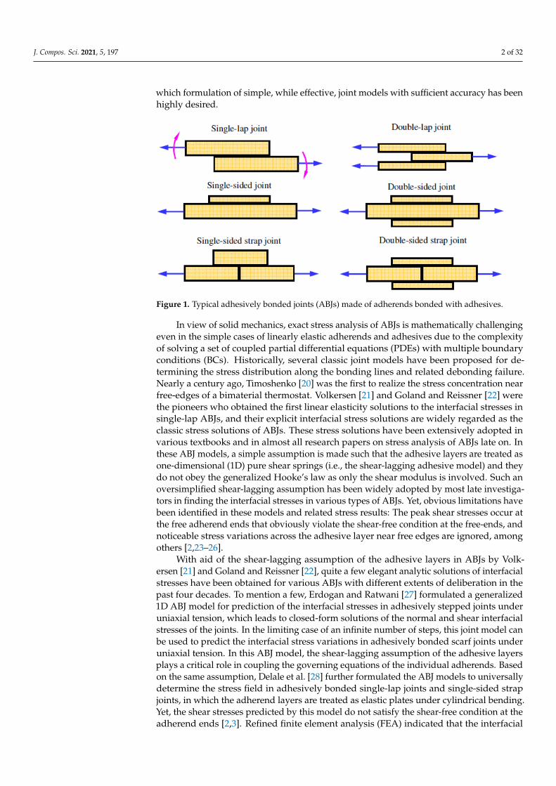
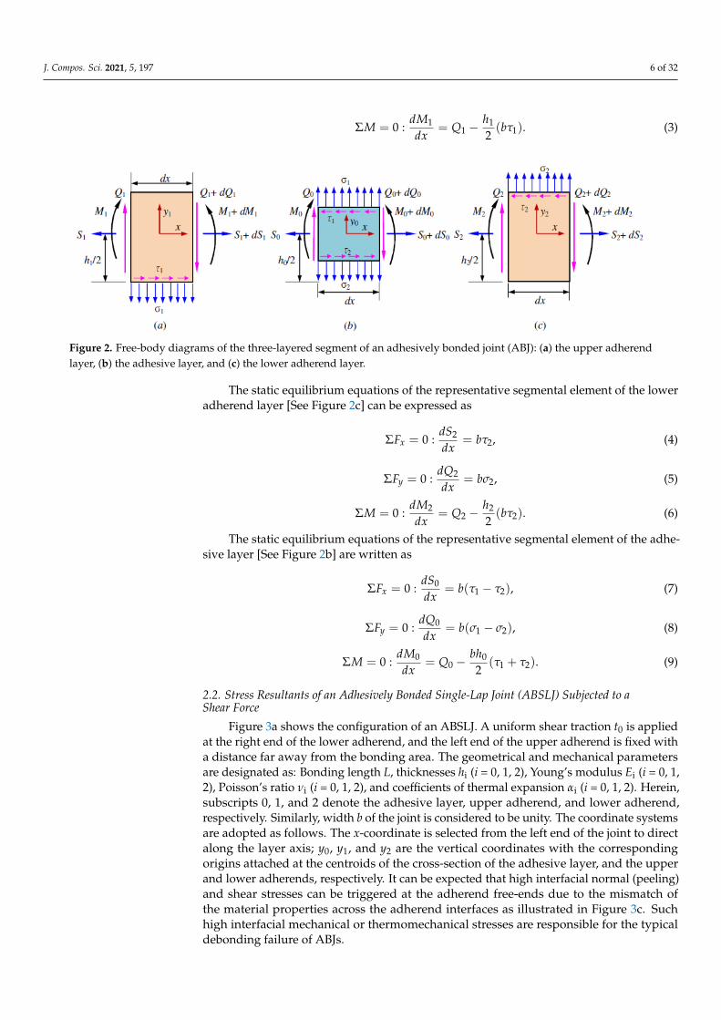
As shown in Figure 1, a typical ABJ consists structurally of three homogeneous, isotrop-ically linearly elastic segments, i.e., one three-layered joint segment and two single-layeredadherend segments, though more structurally complicated ABJs can also be generated viaattaching additional adhesive and adherend layers. The ABJ deformations are assumedsmall, and nonlinear geometrical effects are not considered (such as large deflections). Ingeneral, the two slender adherend segments can be treated simply as two Euler-Bernoullibeams, while accurate stress analysis is challenging in the three-layered joint segment dueto its multiple materials and boundaries subjected to external loads. This three-layeredsegment is the focus in ABJ modeling that has attracted a large number of investigatorsin the past several decades. Herein, the study starts with the accurate stress analysis ofthis three-layered joint segment subjected to external mechanical and thermomechanicalloads. In a general case of ABJs, due to loss of the lateral symmetry, deformations ofthis three-layered segment in an ABJ are a combination of axial elongation and lateraldeflection. The upper/lower adherend and adhesive layers of the joint are assumed to beslender, with the same width b and the thicknesses of h1, h2, and h0, respectively, and theiraxial stresses can be approximated to follow the classic Euler-Bernoulli beam theory whilethe shear and lateral normal stresses are determined according to the static equilibriumequations in 2D elasticity. Free-body diagrams (FBDs) of the representative segments of theupper/lower adherend and adhesive layers are shown in Figure 2a–c, in which the stresscomponents and related stress resultants, i.e., the axial force Si, shear force Qi, and bendingmoment Mi (i = 0, 1, 2), are defined to follow the standard sign conventions designated inelementary mechanics of materials [103]. For the representative segmental element of theupper adherend layer [See Figure 2a], the static equilibrium equations in terms of stressresultants are

ΣFx = 0 :dS1

dx= −bτ1, (1)

ΣFy = 0 :dQ1

dx= −bσ1, (2)

J. Compos. Sci. 2021, 5, 197 6 of 32

ΣM = 0 :dM1

dx= Q1 −

h1

2(bτ1). (3)

J. Compos. Sci. 2021, 5, x FOR PEER REVIEW 6 of 34

tions designated in elementary mechanics of materials [103]. For the representative seg-mental element of the upper adherend layer [See Figure 2a], the static equilibrium equa-tions in terms of stress resultants are

:0=Σ xF 11,dS b

dxτ= − (1)

:0=Σ yF 11,dQ b

dxσ= − (2)

:0=ΣM 1 11 1( ).

2dM hQ bdx

τ= − (3)

Figure 2. Free-body diagrams of the three-layered segment of an adhesively bonded joint (ABJ): (a) the upper adherend layer, (b) the adhesive layer, and (c) the lower adherend layer.

The static equilibrium equations of the representative segmental element of the lower adherend layer [See Figure 2c] can be expressed as

:0=Σ xF 22 ,dS b

dxτ= (4)

:0=Σ yF 22 ,dQ b

dxσ= (5)

:0=ΣM 2 22 2( ).

2dM hQ bdx

τ= − (6)

The static equilibrium equations of the representative segmental element of the ad-hesive layer [See Figure 2b] are written as

:0=Σ xF 01 2( ),dS b

dxτ τ= − (7)

:0=Σ yF 01 2( ),dQ b

dxσ σ= − (8)

:0=ΣM 0 00 1 2( ).

2dM bhQdx

τ τ= − + (9)

Figure 2. Free-body diagrams of the three-layered segment of an adhesively bonded joint (ABJ): (a) the upper adherendlayer, (b) the adhesive layer, and (c) the lower adherend layer.

The static equilibrium equations of the representative segmental element of the loweradherend layer [See Figure 2c] can be expressed as

ΣFx = 0 :dS2

dx= bτ2, (4)

ΣFy = 0 :dQ2

dx= bσ2, (5)

ΣM = 0 :dM2

dx= Q2 −

h2

2(bτ2). (6)

The static equilibrium equations of the representative segmental element of the adhe-sive layer [See Figure 2b] are written as

ΣFx = 0 :dS0

dx= b(τ1 − τ2), (7)

ΣFy = 0 :dQ0

dx= b(σ1 − σ2), (8)

ΣM = 0 :dM0

dx= Q0 −

bh0

2(τ1 + τ2). (9)

2.2. Stress Resultants of an Adhesively Bonded Single-Lap Joint (ABSLJ) Subjected to aShear Force

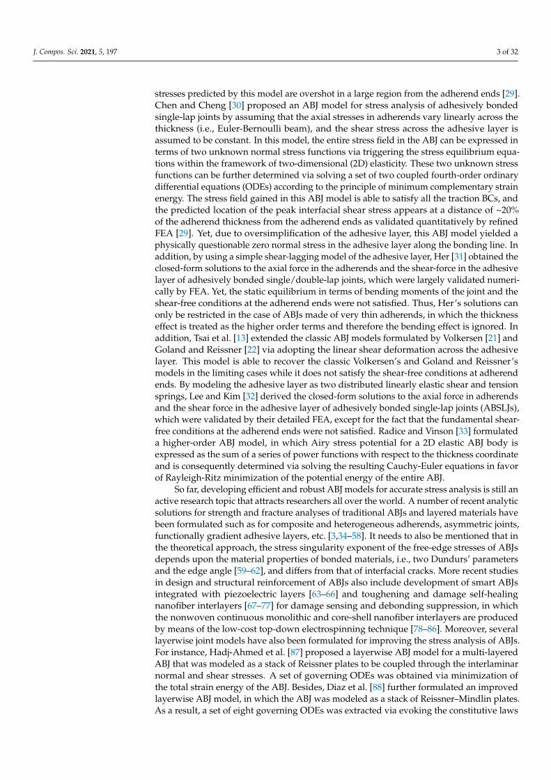
Figure 3a shows the configuration of an ABSLJ. A uniform shear traction t0 is appliedat the right end of the lower adherend, and the left end of the upper adherend is fixed witha distance far away from the bonding area. The geometrical and mechanical parametersare designated as: Bonding length L, thicknesses hi (i = 0, 1, 2), Young’s modulus Ei (i = 0, 1,2), Poisson’s ratio νi (i = 0, 1, 2), and coefficients of thermal expansion αi (i = 0, 1, 2). Herein,subscripts 0, 1, and 2 denote the adhesive layer, upper adherend, and lower adherend,respectively. Similarly, width b of the joint is considered to be unity. The coordinate systemsare adopted as follows. The x-coordinate is selected from the left end of the joint to directalong the layer axis; y0, y1, and y2 are the vertical coordinates with the correspondingorigins attached at the centroids of the cross-section of the adhesive layer, and the upperand lower adherends, respectively. It can be expected that high interfacial normal (peeling)and shear stresses can be triggered at the adherend free-ends due to the mismatch ofthe material properties across the adherend interfaces as illustrated in Figure 3c. Suchhigh interfacial mechanical or thermomechanical stresses are responsible for the typicaldebonding failure of ABJs.

J. Compos. Sci. 2021, 5, 197 7 of 32

J. Compos. Sci. 2021, 5, x FOR PEER REVIEW 8 of 34

,)0( 201 bhtQ = (13c)

,0)(1 =LQ (13d)

1 0 2(0) ,M t bh L= − (13e)

,0)(1 =LM (13f)

,0)0(2 =S (13g)

,0)(2 =LS (13h)

,0)0(2 =Q (13i)

,)( 202 bhtLQ = (13j)

,0)0(2 =M (13k)

,0)(2 =LM (13l)

,0)0(0 =S (13m)

,0)(0 =LS (13n)

,0)0(0 =Q (13o)

,0)(0 =LQ (13p)

,0)0(0 =M (13q)

.0)(0 =LM (13r)

Figure 3. (a) Schematic of an adhesively bonded single-lap joint (ABSLJ) under shearing; (b) the slender upper adherend layer, the adhesive layer, and the slender lower adherend layer; (c) interfa-cial stress distribution in the joint; (d) joint segment used in finite element modeling.

Figure 3. (a) Schematic of an adhesively bonded single-lap joint (ABSLJ) under shearing; (b) theslender upper adherend layer, the adhesive layer, and the slender lower adherend layer; (c) interfacialstress distribution in the joint; (d) joint segment used in finite element modeling.

In reality, ABJs subjected to have mechanical or thermomechanical loads are typicallyin a general three-dimensional (3D) stress state. To simplify the modeling process, in thisstudy the ABJs are treated in the plane-stress state and without residual stresses in theinitial load-free state. Thus, the mechanical and thermomechanical stresses can be treatedseparately according to the method of superposition. In addition, the stress results obtainedin the plane-stress state can be conveniently converted to those in the plane-strain state bysimply replacing the Young’s moduli Ei (i = 0, 1, 2) by (1 − υi

2)/Ei, Poisson’s ratio υi (i = 0,1, 2) by υi/(1 − υi), and coefficients of thermal expansion αi (i = 0, 1, 2) by (1 + υi)αi.

It is the unique feature of the stress-function variational method to define the shearand normal (peeling) stresses at the interface between the upper adherend and the adhesivelayer as two independent interfacial stress functions to be determined:

τ1 = f1(x) and σ1 = g1(x). (10)

Similarly, the interfacial shear and normal (peeling) stresses at the interface betweenthe lower adherend and the adhesive layer are assumed to be another two independentinterfacial stress functions to be determined:

τ2 = f2(x) and σ2 = g2(x). (11)

Thus, the shear-free conditions at the adherend edges at x = 0 and L stand for

f1(0) = f1(L) = 0, (12a)

Andf2(0) = f2(L) = 0. (12b)

J. Compos. Sci. 2021, 5, 197 8 of 32

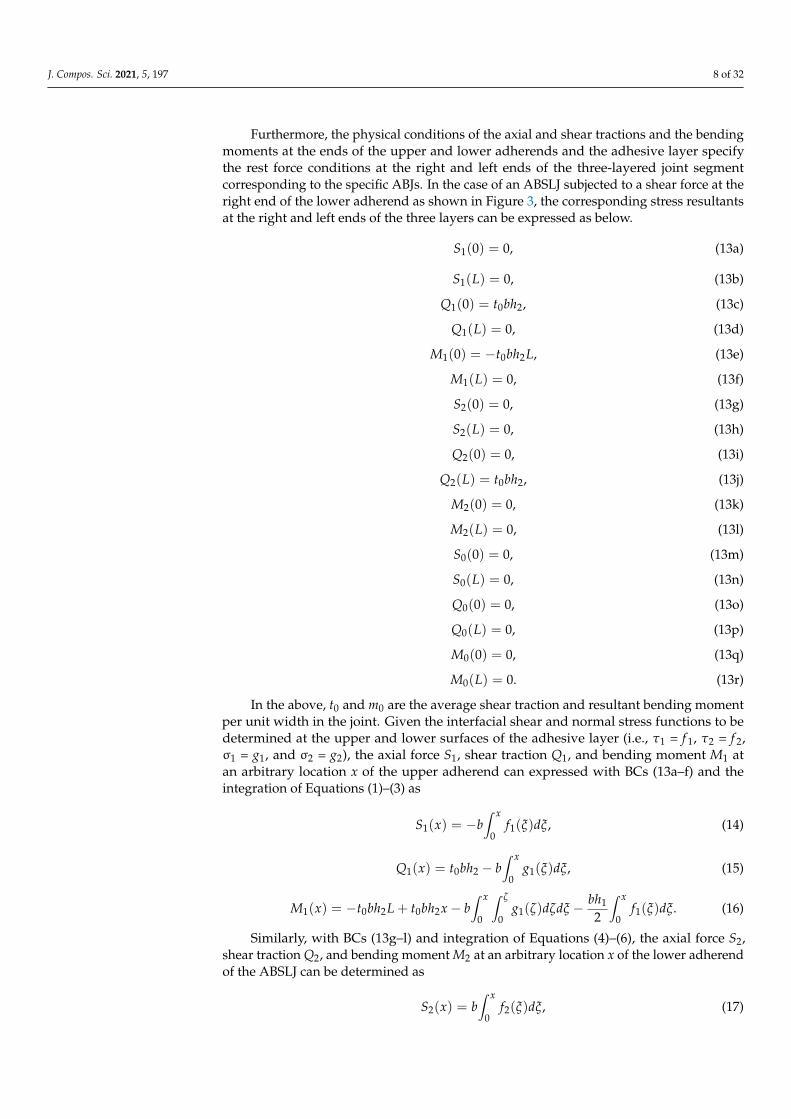
Furthermore, the physical conditions of the axial and shear tractions and the bendingmoments at the ends of the upper and lower adherends and the adhesive layer specifythe rest force conditions at the right and left ends of the three-layered joint segmentcorresponding to the specific ABJs. In the case of an ABSLJ subjected to a shear force at theright end of the lower adherend as shown in Figure 3, the corresponding stress resultantsat the right and left ends of the three layers can be expressed as below.

S1(0) = 0, (13a)

S1(L) = 0, (13b)

Q1(0) = t0bh2, (13c)

Q1(L) = 0, (13d)

M1(0) = −t0bh2L, (13e)

M1(L) = 0, (13f)

S2(0) = 0, (13g)

S2(L) = 0, (13h)

Q2(0) = 0, (13i)

Q2(L) = t0bh2, (13j)

M2(0) = 0, (13k)

M2(L) = 0, (13l)

S0(0) = 0, (13m)

S0(L) = 0, (13n)

Q0(0) = 0, (13o)

Q0(L) = 0, (13p)

M0(0) = 0, (13q)

M0(L) = 0. (13r)

In the above, t0 and m0 are the average shear traction and resultant bending momentper unit width in the joint. Given the interfacial shear and normal stress functions to bedetermined at the upper and lower surfaces of the adhesive layer (i.e., τ1 = f 1, τ2 = f 2,σ1 = g1, and σ2 = g2), the axial force S1, shear traction Q1, and bending moment M1 atan arbitrary location x of the upper adherend can expressed with BCs (13a–f) and theintegration of Equations (1)–(3) as

S1(x) = −b∫ x

0f1(ξ)dξ, (14)

Q1(x) = t0bh2 − b∫ x

0g1(ξ)dξ, (15)

M1(x) = −t0bh2L + t0bh2x− b∫ x

0

∫ ζ

0g1(ζ)dζdξ − bh1

2

∫ x

0f1(ξ)dξ. (16)

Similarly, with BCs (13g–l) and integration of Equations (4)–(6), the axial force S2,shear traction Q2, and bending moment M2 at an arbitrary location x of the lower adherendof the ABSLJ can be determined as

S2(x) = b∫ x

0f2(ξ)dξ, (17)

J. Compos. Sci. 2021, 5, 197 9 of 32

Q2(x) = b∫ x

0g2(ξ)dξ, (18)

M2(x) = b∫ x

0

∫ ζ

0g2(ζ)dζdξ − bh2

2

∫ x

0f2(ξ)dξ. (19)

Furthermore, the axial force S0, shear traction Q0, and bending moment M0 at anarbitrary location x at the adhesive layer can be determined via integrating Equations(7)–(9) with BCs (13m–r) as

S0(x) = b∫ x

0[ f1(ξ)− f2(ξ)]dξ, (20)

Q0(x) = b∫ x

0[g1(ξ)− g2(ξ)]dξ, (21)

M0(x) = b∫ x

0

∫ ζ

0[g1(ζ)− g1(ζ)]dζdξ − bh0

2

∫ x

0[ f1(ξ) + f1(ξ)]dξ. (22)

2.3. Planar Stresses in the Adherends and Adhesive Layer of an ABSLJ

In the process of stress-function variational method, the procedure for determiningthe planar stresses in the adherends and adhesive layers is standardized [2,23–26] suchthat the axial stress in each layer is assumed to be linearly varying according to the classicEuler-Bernoulli beam theory while the corresponding shear and transverse normal stressesare determined to satisfy the 2D static equilibrium equations. Thus, the axial stress of theupper adherend of the ABSLJ can be expressed as

σ(1)xx = S1

bh1− M1y1

I1= − 1

h1

∫ x0 f1(ξ)dξ

+ 12y1h3

1[t0h2L− t0h2x +

∫ x0

∫ ζ0 g1(ζ)dζdξ + h1

2

∫ x0 f1(ξ)dξ],

(23)

The corresponding shear stress τ(1)y1x in the upper adherend can be determined via

integrating the 2D static equilibrium equation:

∂σ(1)xx

∂x+

∂τ(1)y1x

∂y1= 0, (24)

with respect to y1 from an arbitrary location y1 to the top surface at y1 = h1/2:

∫ h1/2

y1

∂σ(1)xx

∂xdy1+

∫ h1/2

y1

∂τ(1)y1x

∂y1dy1 = 0, (25)

which yields

τ(1)y1x = − 1

h1[(

h1

2− y1)−

3h1

(h2

14− y2

1)] f1(x) +6h3

1(

h21

4− y2

1)∫ x

0g1(ξ)dξ − 6

h31(

h21

4− y2

1)t0h2, (26)

where the traction-free BC τ(1)y1x(h1/2) = 0 is evoked. In addition, the transverse normal

stress σ(1)y1y1 in the upper adherend can be further determined via integrating the 2D static

equilibrium equation:∂σ

(1)y1y1

∂y1+

∂τ(1)xy1

∂x= 0, (27)

with respect to y1 from an arbitrary location y1 to the top surface at y1 = h1/2 as

∫ h1/2

y1

∂σ(1)y1y1

∂y1dy1+

∫ h1/2

y1

∂τ(1)xy1

∂xdy1 = 0, (28)

J. Compos. Sci. 2021, 5, 197 10 of 32

which leads to

σ(1)y1y1 = − 1

h1

{[ h1

2 ( h12 − y1)− 1

2 (h2

14 − y2

1)−3h1[

h21

4 ( h12 − y1)− 1

3 (h3

18 − y3

1)]

}f /1 (x)

+ 6h3

1[

h21

4 ( h12 − y1)− 1

3 (h3

18 − y3

1)]g1(x).

(29)

In the integration process above, traction BC σ(1)y1y1(h1/2) = 0 is evoked. Similarly, the

axial normal stress σ(2)xx , shear stress τ

(2)y2x, and transverse normal stress σ

(2)y2y2 in the lower

adherend of the ABSLJ can be determined as

σ(2)xx =

S2

bh2− M2y2

I2=

1h2

∫ x

0f2(ξ)dξ − 12y2

h32

[∫ x

0

∫ ζ

0g2(ζ)dζdξ − h2

2

∫ x

0f2(ξ)dξ], (30)

τ(2)y2x = − 1

h2[(y2 +

h2

2) +

3h2

(y22 −

h22

4)] f2(x) +

6h3

2(y2

2 −h2

24)∫ x

0g2(ξ)dξ, (31)

σ(2)y2y2 = 1

h2

{12 (y

22 −

h22

4 ) + h22 (y2 +

h22 ) + 3

h2[ 1

3 (y32 +

h32

8 )− h22

4 (y2 +h22 )]

}f /2 (x)

− 6h3

2[ 1

3 (y32 +

h32

8 )− h22

4 (y2 +h22 )]g2(x).

(32)

In derivations of (31) and (32), integrations for τ(2)y2x(x, y2) and σ

(2)y2y2(x, y2) are made

with the upper and lower limits as y2 and −h2/2, respectively, and traction BCs ofτ(2)y2x(−h2/2) = 0 and σ

(2)y2y2(−h2/2) = 0 are used.

The axial normal stress σ(0)xx , shear stress τ

(0)y0x, and transverse normal stress τ

(0)y0y0 in the

adhesive layer of the ABSLJ are

σ(0)xx = S0

bh0− M0y0

I0= 1

h0

∫ x0 [ f1(ξ)− f2(ξ)]dξ

− 12y0h3

0

{∫ x0

∫ ζ0 [g1(ζ)− g2(ζ)]dζdξ − h0

2

∫ x0 [ f1(ξ) + f2(ξ)]dξ

},

(33)

τ(0)y0x = − f2(x)− 1

h0(y0 +

h02 )[ f1(x)− f2(x)]− 3

h20(y2

0 −h2

04 )[ f1(x) + f2(x)]

+ 6h3

0(y2

0 −h2

04 )∫ x

0 [g1(ξ)− g2(ξ)]dξ,

(34)

σ(0)y0y0 = g2(x) + (y0 +

h02 ) f /

2 (x) + 1h0[ 1

2 (y20 −

h20

4 ) + h02 (y0 +

h02 )][ f /

1 (x)− f /2 (x)]

+ 3h2

0[ 1

3 (y30 +

h30

8 )− h20

4 (y0 +h02 )][ f /

1 (x) + f /2 (x)]

− 6h3

0[ 1

3 (y30 +

h30

8 )− h20

4 (y0 +h02 )][g1(x)− g2(x)].

(35)

In derivations of (34) and (35), integrations for τ(0)y0x(x, y0) and σ

(0)y0y0(x, y0) are made

with the upper and lower limits as y0 and −h0/2, respectively, and traction BCs ofτ(0)y0x(−h0/2) = − f2(x) and σ

(0)y0y0(−h0/2) = g(x) are used. If setting y0 = h0/2, relations (34)

and (35) are automatically consistent with τ(0)y0x(h0/2) = − f1(x) and σ

(0)y0y0(h0/2) = g1(x),

in which the minus sign prior to f 1(x) is due to the sign conversion of stress components inthe theory of elasticity.

The above derivations of the stress components indicate that with the assumptionof axial normal stresses varying linearly across the adherend and adhesive layers of the

J. Compos. Sci. 2021, 5, 197 11 of 32

ABSLJ, the corresponding statically compatible shear and transverse normal stresses havepiecewise parabolic and cubic distributions across these layers, respectively. In addition,such stress fields satisfy all the traction BCs at the ends of the adherend and adhesive layersand the stress continuity across the interfaces between the adherend and adhesive layers.Such a process can also be conveniently extended for determining the stress components inmulti-layered ABJs.

2.4. Governing Equations of the Interfacial Stress Functions and Their Solution of an ABSLJ

With the planar stress components in the adherend and adhesive layers of the ABSLJ,the total strain energy of the ABSLJ (0 ≤ x ≤ L) can be expressed as [2]

U = b∫ L

0

∫ h1/2−h1/2

{12 [σ

(1)xx ε

(1)xx + σ

(1)yy ε

(1)yy ] +

1+υ1E1

[τ(1)xy1 ]

2}

dxdy1

+ b∫ L

0

∫ h2/2−h2/2

{12 [σ

(2)xx ε

(2)xx + σ

(2)yy ε

(2)yy ] +

1+υ2E2

[τ(2)xy2 ]

2}

dxdy2

+ b∫ L

0

∫ h0/2−h0/2

{12 [σ

(0)xx ε

(0)xx + σ

(0)yy ε

(0)yy ] +

1+υ0E0

[τ(0)xy0 ]

2}

dxdy0.

(36)

In the above, ε(i)xx and ε

(i)yy (i = 0, 1, 2) are the axial and transverse normal strains of

the adhesive layer and the upper and lower adherends, respectively, which are definedaccording to the generalized Hooke’s law of an isotropic, linearly thermoelastic solid (inthe plane-stress state):

ε(i)xx =

1Ei

σ(i)xx −

υiEi

σ(i)yy + αi∆T, (37)

ε(i)yy =

1Ei

σ(i)yy −

υiEi

σ(i)xx + αi∆T, (38)

where αi (i = 0, 1, 2) are coefficients of thermal expansion of the adhesive layer, upper,and lower adherends, respectively, and ∆T is the uniform temperature change of the jointfrom the reference temperature of free thermomechanical stress state. In the present caseof an ABSLJ, strain energy (36) is an energy functional with respect to the four unknowninterfacial stress-functions f i (i = 1, 2) and gi (i = 1, 2) adopted above. According to theoremof minimum complimentary strain energy of an elastic body, the total strain energy (orcomplimentary strain energy) reaches a stationary point at static equilibrium of the presentlinearly elastic ABSLJ (with given tractions at free ends), which corresponds to the necessarycondition in terms of variation of the strain energy (36) with respect to the four unknownstress functions [2,3,23–26]

δU = 0, (39)

i.e.,

δU = b∫ L

0

∫ h1/2−h1/2

{12 [σ

(1)xx δε

(1)xx + δσ

(1)xx ε

(1)xx + σ

(1)yy δε

(1)yy + δσ

(1)yy ε

(1)yy ] +

2(1+υ1)E1

τ(1)xy1 δτ

(1)xy1

}dxdy1

+ b∫ L

0

∫ h2/2−h2/2

{12 [σ

(2)xx δε

(2)xx + δσ

(2)xx ε

(2)xx + σ

(2)yy δε

(2)yy + δσ

(2)yy ε

(2)yy ] +

2(1+υ2)E2

τ(2)xy2 δτ

(2)xy2

}dxdy2

+ b∫ L

0

∫ h0/2−h0/2

{12 [σ

(0)xx δε

(0)xx + δσ

(0)xx ε

(0)xx + σ

(0)yy δε

(0)yy + δσ

(0)yy ε

(0)yy ] +

2(1+υ0)E0

τ(0)xy0 δτ

(0)xy0

}dxdy0.

(40)

where δ is the mathematical variational operator with respect to either f i (i = 1, 2) or gi(i = 1, 2).

By adopting the same notations and procedure as used in our previous studies [2,3,23–26],plugging the stress components (23), (26), (29), and (30)–(35) and normal strains (37) and (38)into (40), and evoking the variational operation and several steps of algebraic simplification,

J. Compos. Sci. 2021, 5, 197 12 of 32

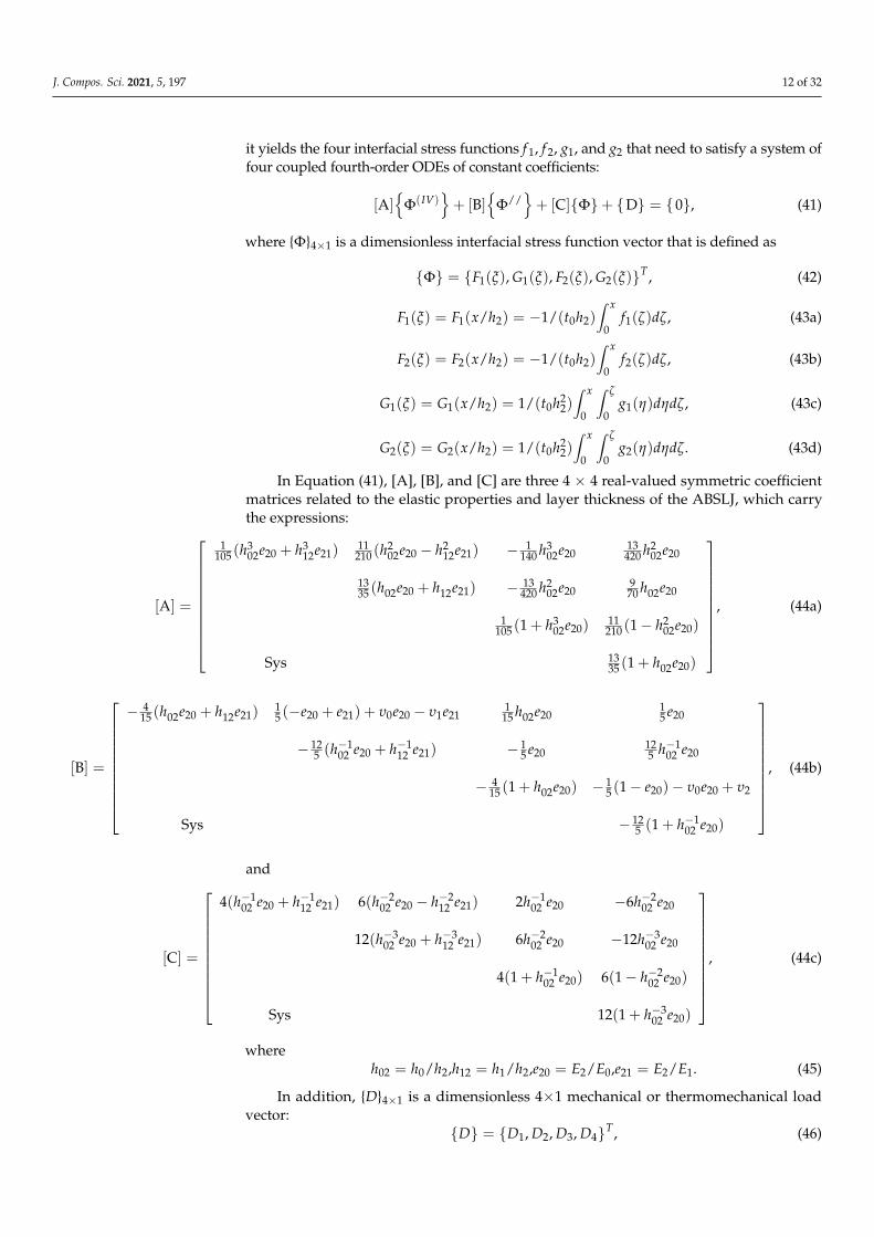
it yields the four interfacial stress functions f 1, f 2, g1, and g2 that need to satisfy a system offour coupled fourth-order ODEs of constant coefficients:

[A]{

Φ(IV)}+ [B]

{Φ//

}+ [C]{Φ}+ {D} = {0}, (41)

where {Φ}4×1 is a dimensionless interfacial stress function vector that is defined as

{Φ} = {F1(ξ), G1(ξ), F2(ξ), G2(ξ)}T , (42)

F1(ξ) = F1(x/h2) = −1/(t0h2)∫ x

0f1(ζ)dζ, (43a)

F2(ξ) = F2(x/h2) = −1/(t0h2)∫ x

0f2(ζ)dζ, (43b)

G1(ξ) = G1(x/h2) = 1/(t0h22)∫ x

0

∫ ζ

0g1(η)dηdζ, (43c)

G2(ξ) = G2(x/h2) = 1/(t0h22)∫ x

0

∫ ζ

0g2(η)dηdζ. (43d)

In Equation (41), [A], [B], and [C] are three 4 × 4 real-valued symmetric coefficientmatrices related to the elastic properties and layer thickness of the ABSLJ, which carrythe expressions:

[A] =

1105 (h

302e20 + h3

12e21)11

210 (h202e20 − h2

12e21) − 1140 h3

02e2013420 h2

02e20

1335 (h02e20 + h12e21) − 13

420 h202e20

970 h02e20

1105 (1 + h3

02e20)11

210 (1− h202e20)

Sys 1335 (1 + h02e20)

, (44a)

[B] =

− 415 (h02e20 + h12e21)

15 (−e20 + e21) + υ0e20 − υ1e21

115 h02e20

15 e20

− 125 (h−1

02 e20 + h−112 e21) − 1

5 e20125 h−1

02 e20

− 415 (1 + h02e20) − 1

5 (1− e20)− υ0e20 + υ2

Sys − 125 (1 + h−1

02 e20)

, (44b)

and

[C] =

4(h−102 e20 + h−1

12 e21) 6(h−202 e20 − h−2

12 e21) 2h−102 e20 −6h−2

02 e20

12(h−302 e20 + h−3

12 e21) 6h−202 e20 −12h−3

02 e20

4(1 + h−102 e20) 6(1− h−2

02 e20)

Sys 12(1 + h−302 e20)

, (44c)

whereh02 = h0/h2,h12 = h1/h2,e20 = E2/E0,e21 = E2/E1. (45)

In addition, {D}4×1 is a dimensionless 4×1 mechanical or thermomechanical loadvector:

{D} = {D1, D2, D3, D4}T , (46)

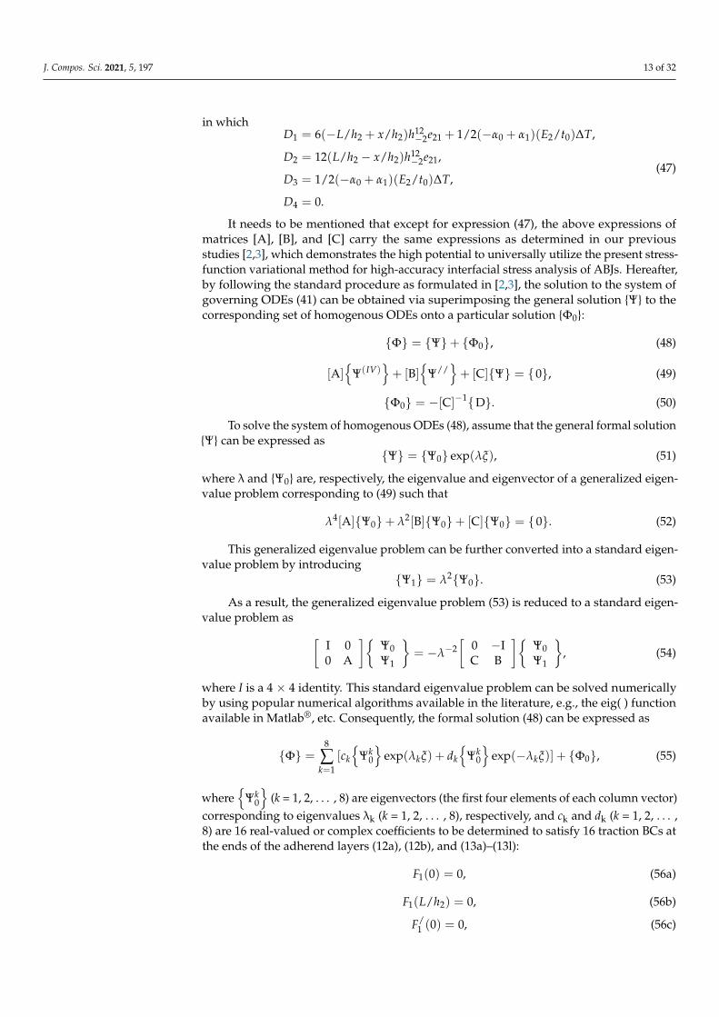
J. Compos. Sci. 2021, 5, 197 13 of 32

in whichD1 = 6(−L/h2 + x/h2)h12

−2e21 + 1/2(−α0 + α1)(E2/t0)∆T,

D2 = 12(L/h2 − x/h2)h12−2e21,

D3 = 1/2(−α0 + α1)(E2/t0)∆T,

D4 = 0.

(47)

It needs to be mentioned that except for expression (47), the above expressions ofmatrices [A], [B], and [C] carry the same expressions as determined in our previousstudies [2,3], which demonstrates the high potential to universally utilize the present stress-function variational method for high-accuracy interfacial stress analysis of ABJs. Hereafter,by following the standard procedure as formulated in [2,3], the solution to the system ofgoverning ODEs (41) can be obtained via superimposing the general solution {Ψ} to thecorresponding set of homogenous ODEs onto a particular solution {Φ0}:

{Φ} = {Ψ}+ {Φ0}, (48)

[A]{

Ψ(IV)}+ [B]

{Ψ//

}+ [C]{Ψ} = {0}, (49)

{Φ0} = −[C]−1{D}. (50)

To solve the system of homogenous ODEs (48), assume that the general formal solution{Ψ} can be expressed as

{Ψ} = {Ψ0} exp(λξ), (51)

where λ and {Ψ0} are, respectively, the eigenvalue and eigenvector of a generalized eigen-value problem corresponding to (49) such that

λ4[A]{Ψ0}+ λ2[B]{Ψ0}+ [C]{Ψ0} = {0}. (52)

This generalized eigenvalue problem can be further converted into a standard eigen-value problem by introducing

{Ψ1} = λ2{Ψ0}. (53)

As a result, the generalized eigenvalue problem (53) is reduced to a standard eigen-value problem as [

I 00 A

]{Ψ0Ψ1

}= −λ−2

[0 −IC B

]{Ψ0Ψ1

}, (54)

where I is a 4 × 4 identity. This standard eigenvalue problem can be solved numericallyby using popular numerical algorithms available in the literature, e.g., the eig( ) functionavailable in Matlab®, etc. Consequently, the formal solution (48) can be expressed as

{Φ} =8

∑k=1

[ck

{Ψk

0

}exp(λkξ) + dk

{Ψk

0

}exp(−λkξ)] + {Φ0}, (55)

where{

Ψk0

}(k = 1, 2, . . . , 8) are eigenvectors (the first four elements of each column vector)

corresponding to eigenvalues λk (k = 1, 2, . . . , 8), respectively, and ck and dk (k = 1, 2, . . . ,8) are 16 real-valued or complex coefficients to be determined to satisfy 16 traction BCs atthe ends of the adherend layers (12a), (12b), and (13a)–(13l):

F1(0) = 0, (56a)

F1(L/h2) = 0, (56b)

F/1 (0) = 0, (56c)

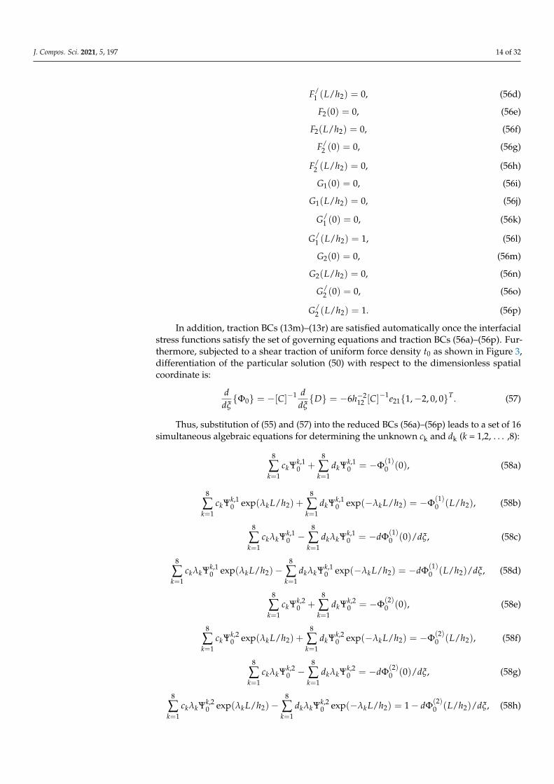
J. Compos. Sci. 2021, 5, 197 14 of 32

F/1 (L/h2) = 0, (56d)

F2(0) = 0, (56e)

F2(L/h2) = 0, (56f)

F/2 (0) = 0, (56g)

F/2 (L/h2) = 0, (56h)

G1(0) = 0, (56i)

G1(L/h2) = 0, (56j)

G/1 (0) = 0, (56k)

G/1 (L/h2) = 1, (56l)

G2(0) = 0, (56m)

G2(L/h2) = 0, (56n)

G/2 (0) = 0, (56o)

G/2 (L/h2) = 1. (56p)

In addition, traction BCs (13m)–(13r) are satisfied automatically once the interfacialstress functions satisfy the set of governing equations and traction BCs (56a)–(56p). Fur-thermore, subjected to a shear traction of uniform force density t0 as shown in Figure 3,differentiation of the particular solution (50) with respect to the dimensionless spatialcoordinate is:

ddξ{Φ0} = −[C]−1 d

dξ{D} = −6h−2

12 [C]−1e21{1,−2, 0, 0}T . (57)

Thus, substitution of (55) and (57) into the reduced BCs (56a)–(56p) leads to a set of 16simultaneous algebraic equations for determining the unknown ck and dk (k = 1,2, . . . ,8):

8

∑k=1

ckΨk,10 +

8

∑k=1

dkΨk,10 = −Φ(1)

0 (0), (58a)

8

∑k=1

ckΨk,10 exp(λkL/h2) +

8

∑k=1

dkΨk,10 exp(−λkL/h2) = −Φ(1)

0 (L/h2), (58b)

8

∑k=1

ckλkΨk,10 −

8

∑k=1

dkλkΨk,10 = −dΦ(1)

0 (0)/dξ, (58c)

8

∑k=1

ckλkΨk,10 exp(λkL/h2)−

8

∑k=1

dkλkΨk,10 exp(−λkL/h2) = −dΦ(1)

0 (L/h2)/dξ, (58d)

8

∑k=1

ckΨk,20 +

8

∑k=1

dkΨk,20 = −Φ(2)

0 (0), (58e)

8

∑k=1

ckΨk,20 exp(λkL/h2) +

8

∑k=1

dkΨk,20 exp(−λkL/h2) = −Φ(2)

0 (L/h2), (58f)

8

∑k=1

ckλkΨk,20 −

8

∑k=1

dkλkΨk,20 = −dΦ(2)

0 (0)/dξ, (58g)

8

∑k=1

ckλkΨk,20 exp(λkL/h2)−

8

∑k=1

dkλkΨk,20 exp(−λkL/h2) = 1− dΦ(2)

0 (L/h2)/dξ, (58h)

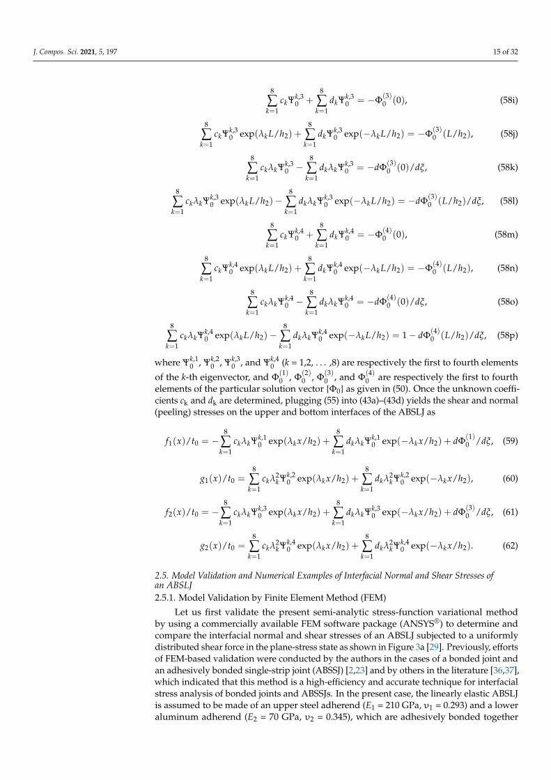
J. Compos. Sci. 2021, 5, 197 15 of 32

8

∑k=1

ckΨk,30 +

8

∑k=1

dkΨk,30 = −Φ(3)

0 (0), (58i)

8

∑k=1

ckΨk,30 exp(λkL/h2) +

8

∑k=1

dkΨk,30 exp(−λkL/h2) = −Φ(3)

0 (L/h2), (58j)

8

∑k=1

ckλkΨk,30 −

8

∑k=1

dkλkΨk,30 = −dΦ(3)

0 (0)/dξ, (58k)

8

∑k=1

ckλkΨk,30 exp(λkL/h2)−

8

∑k=1

dkλkΨk,30 exp(−λkL/h2) = −dΦ(3)

0 (L/h2)/dξ, (58l)

8

∑k=1

ckΨk,40 +

8

∑k=1

dkΨk,40 = −Φ(4)

0 (0), (58m)

8

∑k=1

ckΨk,40 exp(λkL/h2) +

8

∑k=1

dkΨk,40 exp(−λkL/h2) = −Φ(4)

0 (L/h2), (58n)

8

∑k=1

ckλkΨk,40 −

8

∑k=1

dkλkΨk,40 = −dΦ(4)

0 (0)/dξ, (58o)

8

∑k=1

ckλkΨk,40 exp(λkL/h2)−

8

∑k=1

dkλkΨk,40 exp(−λkL/h2) = 1− dΦ(4)

0 (L/h2)/dξ, (58p)

where Ψk,10 , Ψk,2

0 , Ψk,30 , and Ψk,4

0 (k = 1,2, . . . ,8) are respectively the first to fourth elements

of the k-th eigenvector, and Φ(1)0 , Φ(2)

0 , Φ(3)0 , and Φ(4)

0 are respectively the first to fourthelements of the particular solution vector {Φ0} as given in (50). Once the unknown coeffi-cients ck and dk are determined, plugging (55) into (43a)–(43d) yields the shear and normal(peeling) stresses on the upper and bottom interfaces of the ABSLJ as

f1(x)/t0 = −8

∑k=1

ckλkΨk,10 exp(λkx/h2) +

8

∑k=1

dkλkΨk,10 exp(−λkx/h2) + dΦ(1)

0 /dξ, (59)

g1(x)/t0 =8

∑k=1

ckλ2kΨk,2

0 exp(λkx/h2) +8

∑k=1

dkλ2kΨk,2

0 exp(−λkx/h2), (60)

f2(x)/t0 = −8

∑k=1

ckλkΨk,30 exp(λkx/h2) +

8

∑k=1

dkλkΨk,30 exp(−λkx/h2) + dΦ(3)

0 /dξ, (61)

g2(x)/t0 =8

∑k=1

ckλ2kΨk,4

0 exp(λkx/h2) +8

∑k=1

dkλ2kΨk,4

0 exp(−λkx/h2). (62)

2.5. Model Validation and Numerical Examples of Interfacial Normal and Shear Stresses ofan ABSLJ2.5.1. Model Validation by Finite Element Method (FEM)

Let us first validate the present semi-analytic stress-function variational methodby using a commercially available FEM software package (ANSYS®) to determine andcompare the interfacial normal and shear stresses of an ABSLJ subjected to a uniformlydistributed shear force in the plane-stress state as shown in Figure 3a [29]. Previously, effortsof FEM-based validation were conducted by the authors in the cases of a bonded joint andan adhesively bonded single-strip joint (ABSSJ) [2,23] and by others in the literature [36,37],which indicated that this method is a high-efficiency and accurate technique for interfacialstress analysis of bonded joints and ABSSJs. In the present case, the linearly elastic ABSLJis assumed to be made of an upper steel adherend (E1 = 210 GPa, υ1 = 0.293) and a loweraluminum adherend (E2 = 70 GPa, υ2 = 0.345), which are adhesively bonded together

J. Compos. Sci. 2021, 5, 197 16 of 32

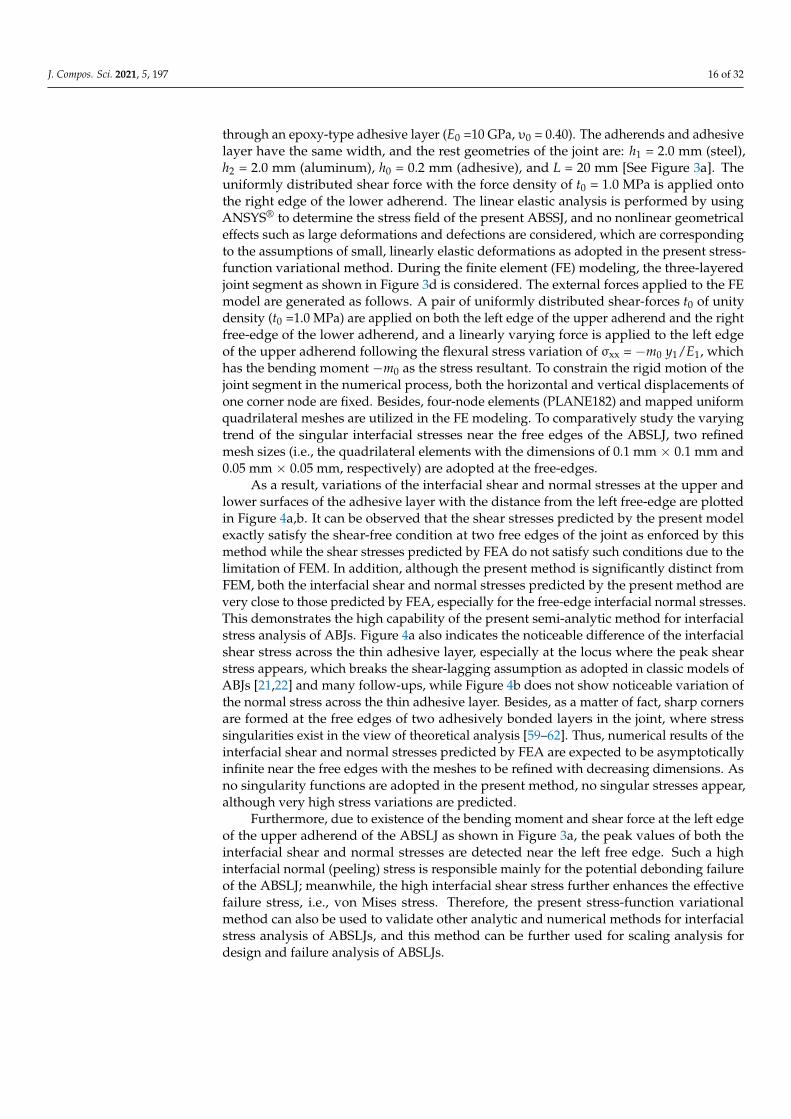
through an epoxy-type adhesive layer (E0 =10 GPa, υ0 = 0.40). The adherends and adhesivelayer have the same width, and the rest geometries of the joint are: h1 = 2.0 mm (steel),h2 = 2.0 mm (aluminum), h0 = 0.2 mm (adhesive), and L = 20 mm [See Figure 3a]. Theuniformly distributed shear force with the force density of t0 = 1.0 MPa is applied ontothe right edge of the lower adherend. The linear elastic analysis is performed by usingANSYS® to determine the stress field of the present ABSSJ, and no nonlinear geometricaleffects such as large deformations and defections are considered, which are correspondingto the assumptions of small, linearly elastic deformations as adopted in the present stress-function variational method. During the finite element (FE) modeling, the three-layeredjoint segment as shown in Figure 3d is considered. The external forces applied to the FEmodel are generated as follows. A pair of uniformly distributed shear-forces t0 of unitydensity (t0 =1.0 MPa) are applied on both the left edge of the upper adherend and the rightfree-edge of the lower adherend, and a linearly varying force is applied to the left edgeof the upper adherend following the flexural stress variation of σxx = −m0 y1/E1, whichhas the bending moment −m0 as the stress resultant. To constrain the rigid motion of thejoint segment in the numerical process, both the horizontal and vertical displacements ofone corner node are fixed. Besides, four-node elements (PLANE182) and mapped uniformquadrilateral meshes are utilized in the FE modeling. To comparatively study the varyingtrend of the singular interfacial stresses near the free edges of the ABSLJ, two refinedmesh sizes (i.e., the quadrilateral elements with the dimensions of 0.1 mm × 0.1 mm and0.05 mm × 0.05 mm, respectively) are adopted at the free-edges.

As a result, variations of the interfacial shear and normal stresses at the upper andlower surfaces of the adhesive layer with the distance from the left free-edge are plottedin Figure 4a,b. It can be observed that the shear stresses predicted by the present modelexactly satisfy the shear-free condition at two free edges of the joint as enforced by thismethod while the shear stresses predicted by FEA do not satisfy such conditions due to thelimitation of FEM. In addition, although the present method is significantly distinct fromFEM, both the interfacial shear and normal stresses predicted by the present method arevery close to those predicted by FEA, especially for the free-edge interfacial normal stresses.This demonstrates the high capability of the present semi-analytic method for interfacialstress analysis of ABJs. Figure 4a also indicates the noticeable difference of the interfacialshear stress across the thin adhesive layer, especially at the locus where the peak shearstress appears, which breaks the shear-lagging assumption as adopted in classic models ofABJs [21,22] and many follow-ups, while Figure 4b does not show noticeable variation ofthe normal stress across the thin adhesive layer. Besides, as a matter of fact, sharp cornersare formed at the free edges of two adhesively bonded layers in the joint, where stresssingularities exist in the view of theoretical analysis [59–62]. Thus, numerical results of theinterfacial shear and normal stresses predicted by FEA are expected to be asymptoticallyinfinite near the free edges with the meshes to be refined with decreasing dimensions. Asno singularity functions are adopted in the present method, no singular stresses appear,although very high stress variations are predicted.

Furthermore, due to existence of the bending moment and shear force at the left edgeof the upper adherend of the ABSLJ as shown in Figure 3a, the peak values of both theinterfacial shear and normal stresses are detected near the left free edge. Such a highinterfacial normal (peeling) stress is responsible mainly for the potential debonding failureof the ABSLJ; meanwhile, the high interfacial shear stress further enhances the effectivefailure stress, i.e., von Mises stress. Therefore, the present stress-function variationalmethod can also be used to validate other analytic and numerical methods for interfacialstress analysis of ABSLJs, and this method can be further used for scaling analysis fordesign and failure analysis of ABSLJs.

J. Compos. Sci. 2021, 5, 197 17 of 32

J. Compos. Sci. 2021, 5, x FOR PEER REVIEW 18 of 34

peak shear stress appears, which breaks the shear-lagging assumption as adopted in clas-sic models of ABJs [21,22] and many follow-ups, while Figure 4b does not show noticeable variation of the normal stress across the thin adhesive layer. Besides, as a matter of fact, sharp corners are formed at the free edges of two adhesively bonded layers in the joint, where stress singularities exist in the view of theoretical analysis [59–62]. Thus, numerical results of the interfacial shear and normal stresses predicted by FEA are expected to be asymptotically infinite near the free edges with the meshes to be refined with decreasing dimensions. As no singularity functions are adopted in the present method, no singular stresses appear, although very high stress variations are predicted.

Furthermore, due to existence of the bending moment and shear force at the left edge of the upper adherend of the ABSLJ as shown in Figure 3a, the peak values of both the interfacial shear and normal stresses are detected near the left free edge. Such a high in-terfacial normal (peeling) stress is responsible mainly for the potential debonding failure of the ABSLJ; meanwhile, the high interfacial shear stress further enhances the effective failure stress, i.e., von Mises stress. Therefore, the present stress-function variational method can also be used to validate other analytic and numerical methods for interfacial stress analysis of ABSLJs, and this method can be further used for scaling analysis for design and failure analysis of ABSLJs.

Figure 4. Validation of the stress-function variational method for determining the interfacial shear and normal stresses in an ABSLJ subjected to a shear traction: (a) Interfacial shear stress and (b) interfacial normal stress at the upper and lower surfaces of the adhesive layer, respectively (In each case, the first four curves are predicted by FEA with indications of the corresponding peak stress values).

2.5.2. Scaling Analysis of Interfacial Shear and Normal Stresses of ABSLJs due to Me-chanical Loads

With the high-efficiency, accurate semi-analytic stress-function variational method developed above, it is convenient to examine the effects of elastic properties and geome-tries of the adherend and adhesive layers on the interfacial shear and normal stresses of the ABSLJ. Below the effects of thickness and Young’s modulus of the adhesive layer on the interfacial shear and normal stresses in the present ABSLJ are investigated. For con-venience of the scaling analysis, the adherend length and Young’s modulus ratios are fixed as L/h2 = 8 and E2/E1 = 1/3 (approximately equal to the ratio of aluminum to steel), and Poisson’s ratios of the upper and lower adherends are fixed as υ1 = 0.293 (steel) and υ2 = 0.345 (aluminum), respectively. For the adhesive layer, four thickness ratios (h0/h2 = 0.1, 0.25, 0.5, and 1.0) and two Young’s modulus ratios (E0/E2 = 1/10 and 1/5) are adopted, and the Poisson’s ratio is fixed at υ0 = 0.4 (thermosetting epoxy) in the entire scaling anal-ysis. The joint is treated in the plane-stress state. Figures 5 and 6 show variations of the normalized interfacial shear stress τ/t0 and normal (peeling) stress σ/t0 at the upper and lower surfaces of the adhesive layer with the dimensionless distance x/h2 from the left to

Figure 4. Validation of the stress-function variational method for determining the interfacial shear and normal stresses inan ABSLJ subjected to a shear traction: (a) Interfacial shear stress and (b) interfacial normal stress at the upper and lowersurfaces of the adhesive layer, respectively (In each case, the first four curves are predicted by FEA with indications of thecorresponding peak stress values).

2.5.2. Scaling Analysis of Interfacial Shear and Normal Stresses of ABSLJs Due toMechanical Loads

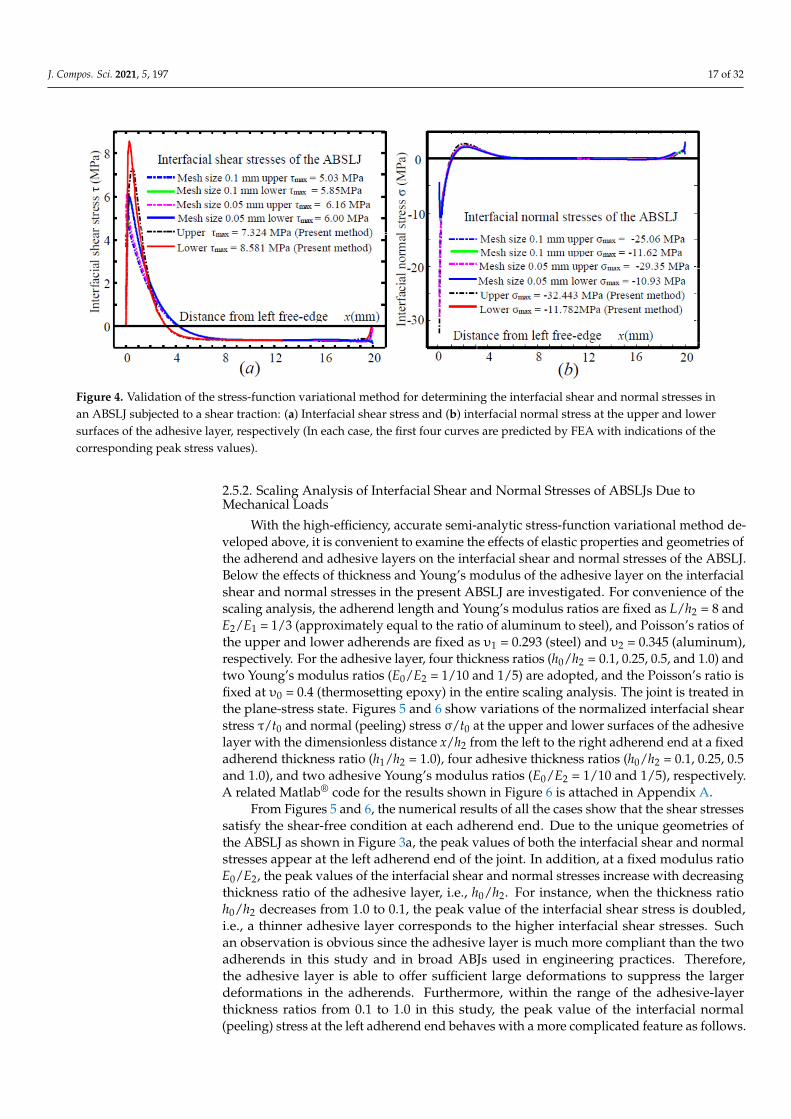
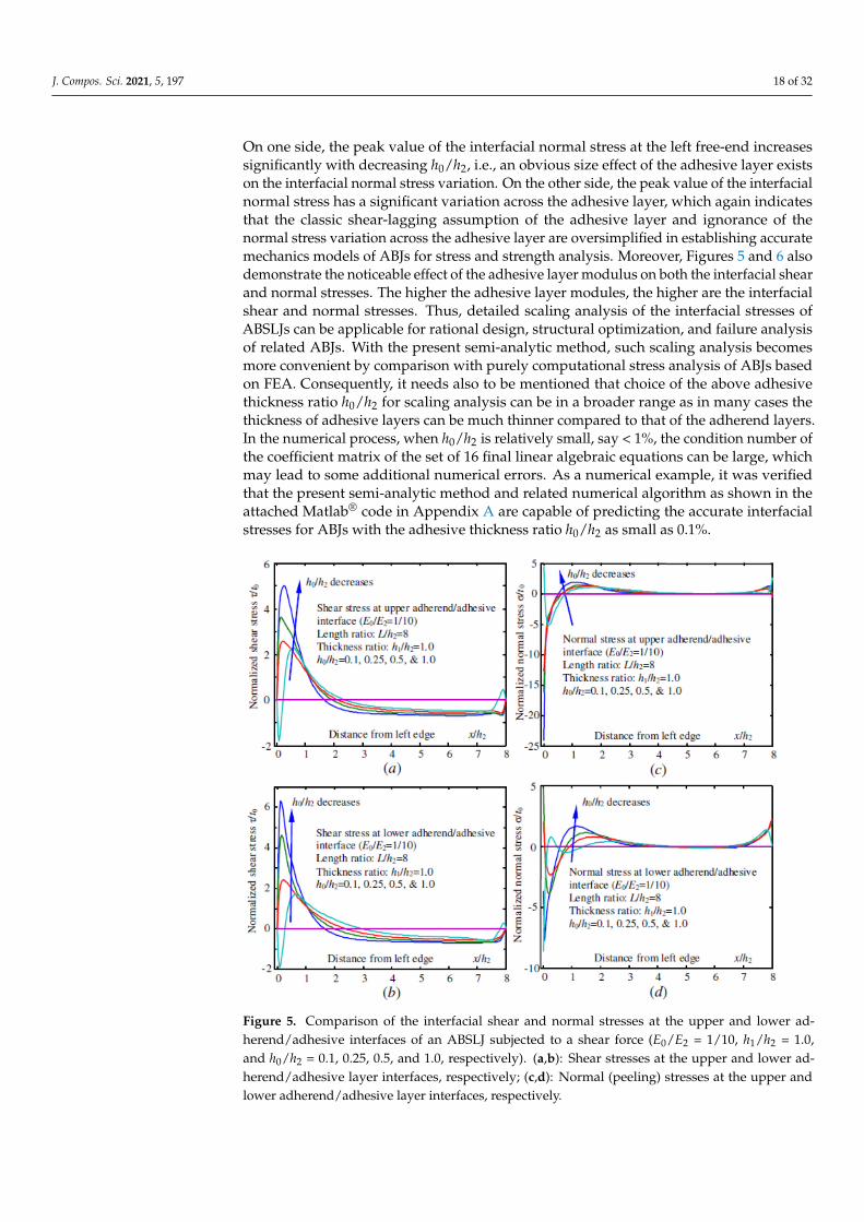
With the high-efficiency, accurate semi-analytic stress-function variational method de-veloped above, it is convenient to examine the effects of elastic properties and geometries ofthe adherend and adhesive layers on the interfacial shear and normal stresses of the ABSLJ.Below the effects of thickness and Young’s modulus of the adhesive layer on the interfacialshear and normal stresses in the present ABSLJ are investigated. For convenience of thescaling analysis, the adherend length and Young’s modulus ratios are fixed as L/h2 = 8 andE2/E1 = 1/3 (approximately equal to the ratio of aluminum to steel), and Poisson’s ratios ofthe upper and lower adherends are fixed as υ1 = 0.293 (steel) and υ2 = 0.345 (aluminum),respectively. For the adhesive layer, four thickness ratios (h0/h2 = 0.1, 0.25, 0.5, and 1.0) andtwo Young’s modulus ratios (E0/E2 = 1/10 and 1/5) are adopted, and the Poisson’s ratio isfixed at υ0 = 0.4 (thermosetting epoxy) in the entire scaling analysis. The joint is treated inthe plane-stress state. Figures 5 and 6 show variations of the normalized interfacial shearstress τ/t0 and normal (peeling) stress σ/t0 at the upper and lower surfaces of the adhesivelayer with the dimensionless distance x/h2 from the left to the right adherend end at a fixedadherend thickness ratio (h1/h2 = 1.0), four adhesive thickness ratios (h0/h2 = 0.1, 0.25, 0.5and 1.0), and two adhesive Young’s modulus ratios (E0/E2 = 1/10 and 1/5), respectively.A related Matlab® code for the results shown in Figure 6 is attached in Appendix A.

From Figures 5 and 6, the numerical results of all the cases show that the shear stressessatisfy the shear-free condition at each adherend end. Due to the unique geometries ofthe ABSLJ as shown in Figure 3a, the peak values of both the interfacial shear and normalstresses appear at the left adherend end of the joint. In addition, at a fixed modulus ratioE0/E2, the peak values of the interfacial shear and normal stresses increase with decreasingthickness ratio of the adhesive layer, i.e., h0/h2. For instance, when the thickness ratioh0/h2 decreases from 1.0 to 0.1, the peak value of the interfacial shear stress is doubled,i.e., a thinner adhesive layer corresponds to the higher interfacial shear stresses. Suchan observation is obvious since the adhesive layer is much more compliant than the twoadherends in this study and in broad ABJs used in engineering practices. Therefore,the adhesive layer is able to offer sufficient large deformations to suppress the largerdeformations in the adherends. Furthermore, within the range of the adhesive-layerthickness ratios from 0.1 to 1.0 in this study, the peak value of the interfacial normal(peeling) stress at the left adherend end behaves with a more complicated feature as follows.

J. Compos. Sci. 2021, 5, 197 18 of 32

On one side, the peak value of the interfacial normal stress at the left free-end increasessignificantly with decreasing h0/h2, i.e., an obvious size effect of the adhesive layer existson the interfacial normal stress variation. On the other side, the peak value of the interfacialnormal stress has a significant variation across the adhesive layer, which again indicatesthat the classic shear-lagging assumption of the adhesive layer and ignorance of thenormal stress variation across the adhesive layer are oversimplified in establishing accuratemechanics models of ABJs for stress and strength analysis. Moreover, Figures 5 and 6 alsodemonstrate the noticeable effect of the adhesive layer modulus on both the interfacial shearand normal stresses. The higher the adhesive layer modules, the higher are the interfacialshear and normal stresses. Thus, detailed scaling analysis of the interfacial stresses ofABSLJs can be applicable for rational design, structural optimization, and failure analysisof related ABJs. With the present semi-analytic method, such scaling analysis becomesmore convenient by comparison with purely computational stress analysis of ABJs basedon FEA. Consequently, it needs also to be mentioned that choice of the above adhesivethickness ratio h0/h2 for scaling analysis can be in a broader range as in many cases thethickness of adhesive layers can be much thinner compared to that of the adherend layers.In the numerical process, when h0/h2 is relatively small, say < 1%, the condition number ofthe coefficient matrix of the set of 16 final linear algebraic equations can be large, whichmay lead to some additional numerical errors. As a numerical example, it was verifiedthat the present semi-analytic method and related numerical algorithm as shown in theattached Matlab® code in Appendix A are capable of predicting the accurate interfacialstresses for ABJs with the adhesive thickness ratio h0/h2 as small as 0.1%.

J. Compos. Sci. 2021, 5, x FOR PEER REVIEW 19 of 34

the right adherend end at a fixed adherend thickness ratio (h1/h2 = 1.0), four adhesive thick-ness ratios (h0/h2 = 0.1, 0.25, 0.5 and 1.0), and two adhesive Young’s modulus ratios (E0/E2 = 1/10 and 1/5), respectively. A related Matlab® code for the results shown in Figure 6 is attached in Appendix A.

Figure 5. Comparison of the interfacial shear and normal stresses at the upper and lower ad-herend/adhesive interfaces of an ABSLJ subjected to a shear force (E0/E2 = 1/10, h1/h2 = 1.0, and h0/h2 = 0.1, 0.25, 0.5, and 1.0, respectively). (a,b): Shear stresses at the upper and lower adherend/adhesive layer interfaces, respectively; (c,d): Normal (peeling) stresses at the upper and lower adherend/ad-hesive layer interfaces, respectively.

Figure 6. Comparison of the interfacial shear and normal stresses at the upper and lower ad-herend/adhesive interfaces subjected to a shear force (E0/E2 = 1/5, h1/h2 = 1.0, and h0/h2 = 0.1, 0.25, 0.5,

Figure 5. Comparison of the interfacial shear and normal stresses at the upper and lower ad-herend/adhesive interfaces of an ABSLJ subjected to a shear force (E0/E2 = 1/10, h1/h2 = 1.0,and h0/h2 = 0.1, 0.25, 0.5, and 1.0, respectively). (a,b): Shear stresses at the upper and lower ad-herend/adhesive layer interfaces, respectively; (c,d): Normal (peeling) stresses at the upper andlower adherend/adhesive layer interfaces, respectively.

J. Compos. Sci. 2021, 5, 197 19 of 32

J. Compos. Sci. 2021, 5, x FOR PEER REVIEW 19 of 34

the right adherend end at a fixed adherend thickness ratio (h1/h2 = 1.0), four adhesive thick-ness ratios (h0/h2 = 0.1, 0.25, 0.5 and 1.0), and two adhesive Young’s modulus ratios (E0/E2 = 1/10 and 1/5), respectively. A related Matlab® code for the results shown in Figure 6 is attached in Appendix A.

Figure 5. Comparison of the interfacial shear and normal stresses at the upper and lower ad-herend/adhesive interfaces of an ABSLJ subjected to a shear force (E0/E2 = 1/10, h1/h2 = 1.0, and h0/h2 = 0.1, 0.25, 0.5, and 1.0, respectively). (a,b): Shear stresses at the upper and lower adherend/adhesive layer interfaces, respectively; (c,d): Normal (peeling) stresses at the upper and lower adherend/ad-hesive layer interfaces, respectively.

Figure 6. Comparison of the interfacial shear and normal stresses at the upper and lower ad-herend/adhesive interfaces subjected to a shear force (E0/E2 = 1/5, h1/h2 = 1.0, and h0/h2 = 0.1, 0.25, 0.5,

Figure 6. Comparison of the interfacial shear and normal stresses at the upper and lower ad-herend/adhesive interfaces subjected to a shear force (E0/E2 = 1/5, h1/h2 = 1.0, and h0/h2 = 0.1, 0.25,0.5, and 1.0, respectively). (a,b): Shear stresses at the upper and lower adherend/adhesive layerinterfaces, respectively; (c,d): Normal (peeling) stresses at the upper and lower adherend/adhesivelayer interfaces, respectively.

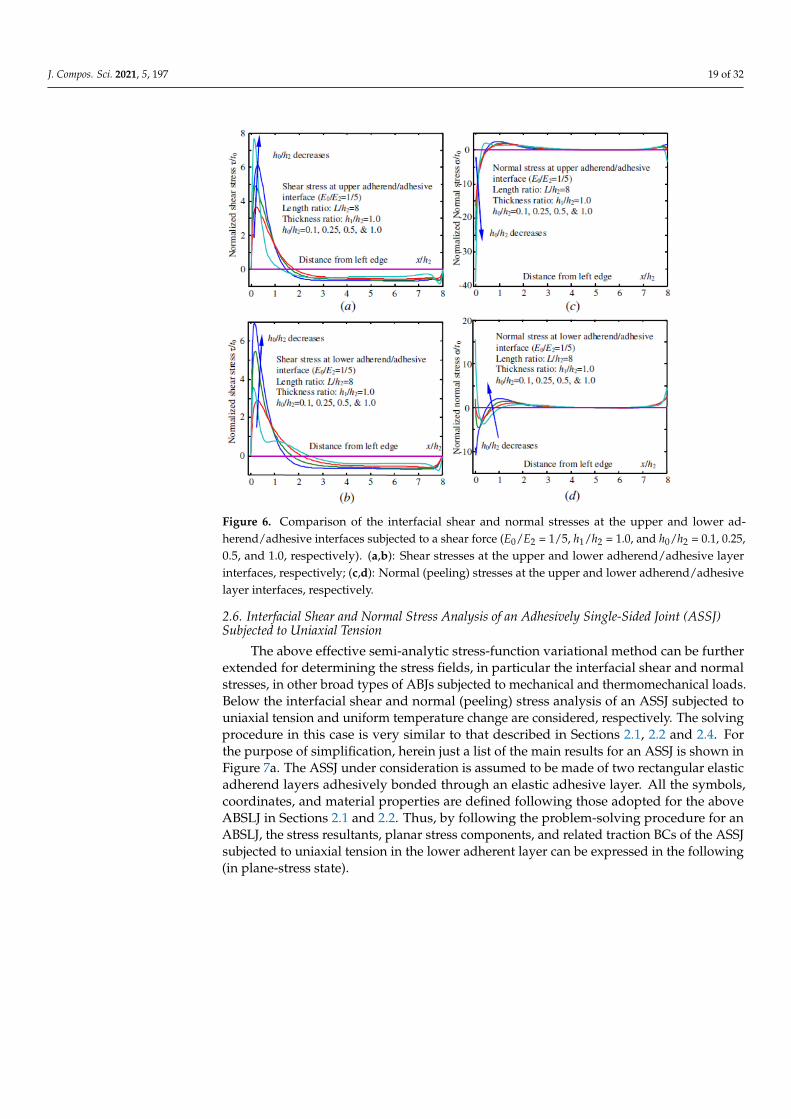
2.6. Interfacial Shear and Normal Stress Analysis of an Adhesively Single-Sided Joint (ASSJ)Subjected to Uniaxial Tension

The above effective semi-analytic stress-function variational method can be furtherextended for determining the stress fields, in particular the interfacial shear and normalstresses, in other broad types of ABJs subjected to mechanical and thermomechanical loads.Below the interfacial shear and normal (peeling) stress analysis of an ASSJ subjected touniaxial tension and uniform temperature change are considered, respectively. The solvingprocedure in this case is very similar to that described in Sections 2.1, 2.2 and 2.4. Forthe purpose of simplification, herein just a list of the main results for an ASSJ is shown inFigure 7a. The ASSJ under consideration is assumed to be made of two rectangular elasticadherend layers adhesively bonded through an elastic adhesive layer. All the symbols,coordinates, and material properties are defined following those adopted for the aboveABSLJ in Sections 2.1 and 2.2. Thus, by following the problem-solving procedure for anABSLJ, the stress resultants, planar stress components, and related traction BCs of the ASSJsubjected to uniaxial tension in the lower adherent layer can be expressed in the following(in plane-stress state).

J. Compos. Sci. 2021, 5, 197 20 of 32

J. Compos. Sci. 2021, 5, x FOR PEER REVIEW 21 of 34

ABSLJ in Sections 2.1–2.2. Thus, by following the problem-solving procedure for an AB-SLJ, the stress resultants, planar stress components, and related traction BCs of the ASSJ subjected to uniaxial tension in the lower adherent layer can be expressed in the following (in plane-stress state).

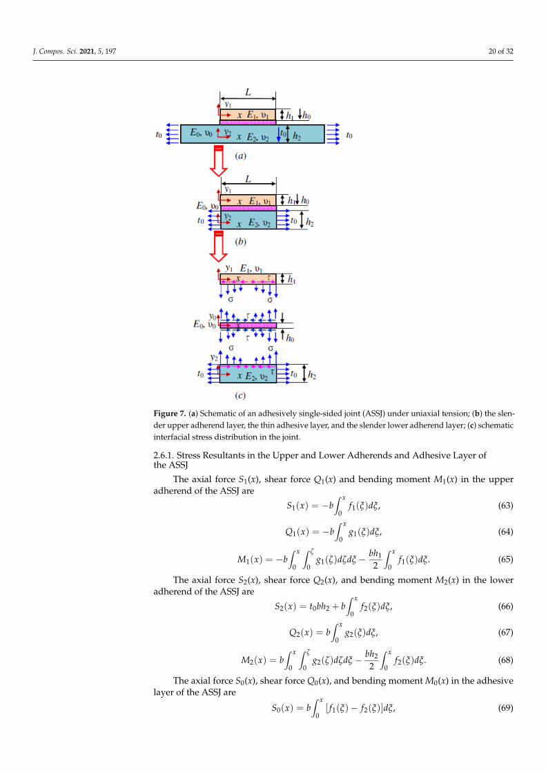
Figure 7. (a) Schematic of an adhesively single-sided joint (ASSJ) under uniaxial tension; (b) the slender upper adherend layer, the thin adhesive layer, and the slender lower adherend layer; (c) schematic interfacial stress distribution in the joint.

2.6.1. Stress Resultants in the Upper and Lower Adherends and Adhesive Layer of the ASSJ

The axial force S1(x), shear force Q1(x) and bending moment M1(x) in the upper ad-herend of the ASSJ are

,)()(0 11 −=x

dfbxS ξξ (63)

1 10( ) ( ) ,

xQ x b g dξ ξ= − (64)

11 1 10 0 0( ) ( ) ( ) .

2x xbhM x b g d d f d

ζζ ζ ξ ξ ξ= − − (65)

The axial force S2(x), shear force Q2(x), and bending moment M2(x) in the lower ad-herend of the ASSJ are

2 0 2 20( ) ( ) ,

xS x t bh b f dξ ξ= + (66)

,)()(0 22 =x

dgbxQ ξξ

(67)

Figure 7. (a) Schematic of an adhesively single-sided joint (ASSJ) under uniaxial tension; (b) the slen-der upper adherend layer, the thin adhesive layer, and the slender lower adherend layer; (c) schematicinterfacial stress distribution in the joint.

2.6.1. Stress Resultants in the Upper and Lower Adherends and Adhesive Layer ofthe ASSJ

The axial force S1(x), shear force Q1(x) and bending moment M1(x) in the upperadherend of the ASSJ are

S1(x) = −b∫ x

0f1(ξ)dξ, (63)

Q1(x) = −b∫ x

0g1(ξ)dξ, (64)

M1(x) = −b∫ x

0

∫ ζ

0g1(ζ)dζdξ − bh1

2

∫ x

0f1(ξ)dξ. (65)

The axial force S2(x), shear force Q2(x), and bending moment M2(x) in the loweradherend of the ASSJ are

S2(x) = t0bh2 + b∫ x

0f2(ξ)dξ, (66)

Q2(x) = b∫ x

0g2(ξ)dξ, (67)

M2(x) = b∫ x

0

∫ ζ

0g2(ζ)dζdξ − bh2

2

∫ x

0f2(ξ)dξ. (68)

The axial force S0(x), shear force Q0(x), and bending moment M0(x) in the adhesivelayer of the ASSJ are

S0(x) = b∫ x

0[ f1(ξ)− f2(ξ)]dξ, (69)

J. Compos. Sci. 2021, 5, 197 21 of 32

Q0(x) = b∫ x

0[g1(ξ)− g2(ξ)]dξ, (70)

M0(x) = b∫ x

0

∫ ζ

0[g1(ζ)− g1(ζ)]dζdξ − bh0

2

∫ x

0[ f1(ξ) + f1(ξ)]dξ. (71)

2.6.2. Planar Stress Components in the Adherends and Adhesive Layer of the ASSJ

The planar axial normal stress σ(1)xx , shear stress τ

(1)xy1 , and lateral normal stress σ

(1)y1y1 in

the upper adherend of the ASSJ are

σ(1)xx =

S1

bh1− M1y1

I1= − 1

h1

∫ x

0f1(ξ)dξ +

12y1

h31

[∫ x

0

∫ ζ

0g1(ζ)dζdξ +

h1

2

∫ x

0f1(ξ)dξ], (72)

τ(1)y1x = − 1

h1[(

h1

2− y1)−

3h1

(h2

14− y2

1)] f1(x) +6h3

1(

h21

4− y2

1)∫ x

0g1(ξ)dξ, (73)

σ(1)y1y1 = − 1

h1

{[ h1

2 ( h12 − y1)− 1

2 (h2

14 − y2

1)−3h1[

h21

4 ( h12 − y1)− 1

3 (h3

18 − y3

1)]

}f /1 (x)

+ 6h3

1[

h21

4 ( h12 − y1)− 1

3 (h3

18 − y3

1)]g1(x).(74)

The planar axial normal stress σ(2)xx , shear stress τ

(2)xy2 , and lateral normal stress σ

(2)y2y2 in

the lower adherend of the ASSJ are

σ(2)xx =

S2

bh2− M2y2

I2= σ0 +

1h2

∫ x

0f2(ξ)dξ − 12y2

h32

[∫ x

0

∫ ζ

0g2(ζ)dζdξ − h2

2

∫ x

0f2(ξ)dξ], (75)

τ(2)y2x = − 1

h2[(y2 +

h2

2) +

3h2

(y22 −

h22

4)] f2(x) +

6h3

2(y2

2 −h2

24)∫ x

0g2(ξ)dξ, (76)

σ(2)y2y2 = 1

h2

{12 (y

22 −

h22

4 ) + h22 (y2 +

h22 ) + 3

h2[ 1

3 (y32 +

h32

8 )− h22

4 (y2 +h22 )]

}f /2 (x)

− 6h3

2[ 1

3 (y32 +

h32

8 )− h22

4 (y2 +h22 )]g2(x).

(77)

The planar axial normal stress σ(0)xx , shear stress τ

(0)xy1 , and lateral normal stress σ

(0)y1y1 in

the adhesive layer of the ASSJ are

σ(0)xx = S0

bh0− M0y0

I0= 1

h0

∫ x0 [ f1(ξ)− f2(ξ)]dξ

− 12y0h3

0

{∫ x0

∫ ζ0 [g1(ζ)− g2(ζ)]dζdξ − h0

2

∫ x0 [ f1(ξ) + f2(ξ)]dξ

},

(78)

τ(0)y0x = − f2(x)− 1

h0(y0 +

h02 )[ f1(x)− f2(x)]− 3

h20(y2

0 −h2

04 )[ f1(x) + f2(x)]

+ 6h3

0(y2

0 −h2

04 )∫ x

0 [g1(ξ)− g2(ξ)]dξ,(79)

σ(0)y0y0 = g2(x) + (y0 +

h02 ) f /

2 (x) + 1h0[ 1

2 (y20 −

h20

4 ) + h02 (y0 +

h02 )][ f /

1 (x)− f /2 (x)]

+ 3h2

0[ 1

3 (y30 +

h30

8 )− h20

4 (y0 +h02 )][ f /

1 (x) + f /2 (x)]

− 6h3

0[ 1

3 (y30 +

h30

8 )− h20

4 (y0 +h02 )][g1(x)− g2(x)].

(80)

Again, by evoking the principle of minimum complimentary strain energy of the ASSJas demonstrated in Section 2.4, it again results in the governing ODE (41) with the same

J. Compos. Sci. 2021, 5, 197 22 of 32

coefficient matrices A, B, and C as given in (44), while the matrix D in (47) is modified as thefollowing. {D}4×1 is a dimensionless 4 × 1 mechanical or thermomechanical load vector:

{D} = {D1, D2, D3, D4}T , (81)

withD1 = (1/2)(−α0 + α1)(E2/t0)∆T,

D2 = 0,

D3 = −1 + (1/2)(−α2 + α0)(E2/t0)∆T,

D4 = 0.

(82)

The particular solution to the governing ODE (43) and its derivative in this case ofASSJ are

{Φ0} = −[C]−1{D}, d{Φ0}/dξ = 0. (83)

Correspondingly, the traction BCs for the governing ODE (41) of the current ASSJ canbe expressed as

F1(0) = 0, (84a)

F1(L/h2) = 0, (84b)

F/1 (0) = 0, (84c)

F/1 (L/h2) = 0, (84d)

F2(0) = 0, (84e)

F2(L/h2) = 0, (84f)

F/2 (0) = 0, (84g)

F/2 (L/h2) = 0, (84h)

G1(0) = 0, (84i)

G1(L/h2) = 0, (84j)

G/1 (0) = 0, (84k)

G/1 (L/h2) = 0, (84l)

G2(0) = 0, (84m)

G2(L/h2) = 0, (84n)

G/2 (0) = 0, (84o)

G/2 (L/h2) = 0. (84p)

The rest procedure for solving the interfacial stress functions for an ASSJ is the sameas that for an ABSLJ as aforementioned. Thus, the numerical solutions for the interfacialshear and normal stresses in an ASSJ can be conveniently determined via modifying therelevant terms in the Matlab® code as given in Appendix A, which again demonstrates thehigh efficiency and universality of the stress-function variational method for interfacialstress analysis of various types of ABJs.

2.6.3. Model Validation and Numerical Examples of Interfacial Shear and Normal Stressesof an ASSJ Subjected to Uniaxial TensionModel Validation by Finite Element Method (FEM)

Similar to Section 2.5.1, the FEM software package ANSYS® is further utilized for vali-dating the stress-function variational method for ASSJs. Detailed computational processesbased on ANSYS® for the present ASSJ are the same as demonstrated in Section 2.5.1. The

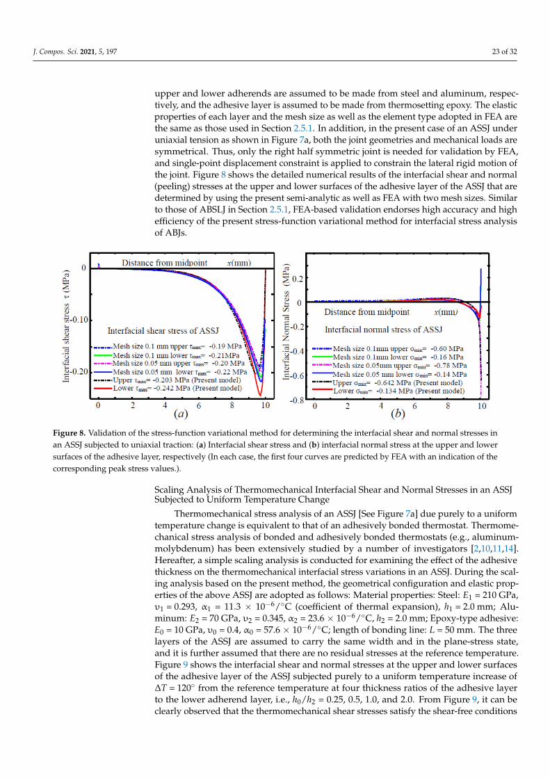
J. Compos. Sci. 2021, 5, 197 23 of 32

upper and lower adherends are assumed to be made from steel and aluminum, respec-tively, and the adhesive layer is assumed to be made from thermosetting epoxy. The elasticproperties of each layer and the mesh size as well as the element type adopted in FEA arethe same as those used in Section 2.5.1. In addition, in the present case of an ASSJ underuniaxial tension as shown in Figure 7a, both the joint geometries and mechanical loads aresymmetrical. Thus, only the right half symmetric joint is needed for validation by FEA,and single-point displacement constraint is applied to constrain the lateral rigid motion ofthe joint. Figure 8 shows the detailed numerical results of the interfacial shear and normal(peeling) stresses at the upper and lower surfaces of the adhesive layer of the ASSJ that aredetermined by using the present semi-analytic as well as FEA with two mesh sizes. Similarto those of ABSLJ in Section 2.5.1, FEA-based validation endorses high accuracy and highefficiency of the present stress-function variational method for interfacial stress analysisof ABJs.

J. Compos. Sci. 2021, 5, x FOR PEER REVIEW 25 of 34

Figure 8. Validation of the stress-function variational method for determining the interfacial shear and normal stresses in an ASSJ subjected to uniaxial traction: (a) Interfacial shear stress and (b) interfacial normal stress at the upper and lower surfaces of the adhesive layer, respectively (In each case, the first four curves are predicted by FEA with an indication of the corresponding peak stress values.).

Scaling Analysis of Thermomechanical Interfacial Shear and Normal Stresses in an ASSJ Subjected to Uniform Temperature Change

Thermomechanical stress analysis of an ASSJ [See Figure 7a] due purely to a uniform temperature change is equivalent to that of an adhesively bonded thermostat. Thermome-chanical stress analysis of bonded and adhesively bonded thermostats (e.g., aluminum-molybdenum) has been extensively studied by a number of investigators [2,10,11,14]. Hereafter, a simple scaling analysis is conducted for examining the effect of the adhesive thickness on the thermomechanical interfacial stress variations in an ASSJ. During the scaling analysis based on the present method, the geometrical configuration and elastic properties of the above ASSJ are adopted as follows: Material properties: Steel: E1 = 210 GPa, υ1 = 0.293, α1 = 11.3 × 10−6/°C (coefficient of thermal expansion), h1 = 2.0 mm; Alumi-num: E2 = 70 GPa, υ2 = 0.345, α2 = 23.6 × 10−6/°C, h2 = 2.0 mm; Epoxy-type adhesive: E0 = 10 GPa, υ0 = 0.4, α0 = 57.6 × 10−6/°C; length of bonding line: L = 50 mm. The three layers of the ASSJ are assumed to carry the same width and in the plane-stress state, and it is further assumed that there are no residual stresses at the reference temperature. Figure 9 shows the interfacial shear and normal stresses at the upper and lower surfaces of the adhesive layer of the ASSJ subjected purely to a uniform temperature increase of ΔT = 120o from the reference temperature at four thickness ratios of the adhesive layer to the lower adherend layer, i.e., h0/h2 = 0.25, 0.5, 1.0, and 2.0. From Figure 9, it can be clearly observed that the thermomechanical shear stresses satisfy the shear-free conditions at the two free edges of the ASSJ. Both high interfacial shear and normal (peeling) stresses are highly localized near the free-edges, where debonding failure most likely happens, and these interfacial shear and normal stresses decay rapidly at the locations off the free edges. In addition, in each case, both the interfacial shear and normal stresses increase with increasing thickness ratio h0/h2 of the adhesive layer, i.e., a relatively thicker adhesive layer corresponds to higher stress concentrations near the free edges. This is due to the fact that the adhesive layer carries a much higher coefficient of thermal expansion. At a fixed temperature change ΔT, a thicker adhesive layer yields higher mismatch deformations between the adhesive layer and either the upper or lower adherend layer of the ASSJ, i.e., higher mis-match strains and high interfacial stresses. Furthermore, the peak value of the peeling stress is nearly double that of the interfacial shear stress at the free edges, thus this ther-momechanical peeling stress is responsible mainly for the debonding failure. In microe-lectronics packaging, the high mismatch of the coefficients of thermal expansion between chips and binding polymers commonly leads to the high thermomechanical stresses, which are responsible for the thermomechanical fatigue failure of microelectronic sys-tems. It needs to also be mentioned that as the present analysis is based on a linearly elastic

Figure 8. Validation of the stress-function variational method for determining the interfacial shear and normal stresses inan ASSJ subjected to uniaxial traction: (a) Interfacial shear stress and (b) interfacial normal stress at the upper and lowersurfaces of the adhesive layer, respectively (In each case, the first four curves are predicted by FEA with an indication of thecorresponding peak stress values.).

Scaling Analysis of Thermomechanical Interfacial Shear and Normal Stresses in an ASSJSubjected to Uniform Temperature Change

Thermomechanical stress analysis of an ASSJ [See Figure 7a] due purely to a uniformtemperature change is equivalent to that of an adhesively bonded thermostat. Thermome-chanical stress analysis of bonded and adhesively bonded thermostats (e.g., aluminum-molybdenum) has been extensively studied by a number of investigators [2,10,11,14].Hereafter, a simple scaling analysis is conducted for examining the effect of the adhesivethickness on the thermomechanical interfacial stress variations in an ASSJ. During the scal-ing analysis based on the present method, the geometrical configuration and elastic prop-erties of the above ASSJ are adopted as follows: Material properties: Steel: E1 = 210 GPa,υ1 = 0.293, α1 = 11.3 × 10−6/◦C (coefficient of thermal expansion), h1 = 2.0 mm; Alu-minum: E2 = 70 GPa, υ2 = 0.345, α2 = 23.6 × 10−6/◦C, h2 = 2.0 mm; Epoxy-type adhesive:E0 = 10 GPa, υ0 = 0.4, α0 = 57.6 × 10−6/◦C; length of bonding line: L = 50 mm. The threelayers of the ASSJ are assumed to carry the same width and in the plane-stress state,and it is further assumed that there are no residual stresses at the reference temperature.Figure 9 shows the interfacial shear and normal stresses at the upper and lower surfacesof the adhesive layer of the ASSJ subjected purely to a uniform temperature increase of∆T = 120◦ from the reference temperature at four thickness ratios of the adhesive layerto the lower adherend layer, i.e., h0/h2 = 0.25, 0.5, 1.0, and 2.0. From Figure 9, it can beclearly observed that the thermomechanical shear stresses satisfy the shear-free conditions

J. Compos. Sci. 2021, 5, 197 24 of 32

at the two free edges of the ASSJ. Both high interfacial shear and normal (peeling) stressesare highly localized near the free-edges, where debonding failure most likely happens,and these interfacial shear and normal stresses decay rapidly at the locations off the freeedges. In addition, in each case, both the interfacial shear and normal stresses increasewith increasing thickness ratio h0/h2 of the adhesive layer, i.e., a relatively thicker adhesivelayer corresponds to higher stress concentrations near the free edges. This is due to the factthat the adhesive layer carries a much higher coefficient of thermal expansion. At a fixedtemperature change ∆T, a thicker adhesive layer yields higher mismatch deformationsbetween the adhesive layer and either the upper or lower adherend layer of the ASSJ, i.e.,higher mismatch strains and high interfacial stresses. Furthermore, the peak value of thepeeling stress is nearly double that of the interfacial shear stress at the free edges, thusthis thermomechanical peeling stress is responsible mainly for the debonding failure. Inmicroelectronics packaging, the high mismatch of the coefficients of thermal expansion be-tween chips and binding polymers commonly leads to the high thermomechanical stresses,which are responsible for the thermomechanical fatigue failure of microelectronic systems.It needs to also be mentioned that as the present analysis is based on a linearly elastic ASSJmodel, all predicted interfacial shear and normal stress only depend on the thickness andmodulus ratios. Therefore, the present stress-function variational method also demon-strates the great potential for efficient and accurate thermomechanical interfacial stressanalysis of ABJs and adhesively bonded thermostats.

J. Compos. Sci. 2021, 5, x FOR PEER REVIEW 26 of 34

ASSJ model, all predicted interfacial shear and normal stress only depend on the thickness and modulus ratios. Therefore, the present stress-function variational method also demonstrates the great potential for efficient and accurate thermomechanical interfacial stress analysis of ABJs and adhesively bonded thermostats.

Figure 9. Comparison of thermomechanical interfacial shear and normal stresses at the upper and bottom surface of the adhesive layer of an ASSJ subjected to uniform temperature change (ΔT = 120 °C; E1/E2 = 1/3; E0/E2 = 1/7; L/h2 = 20; h1/h2 = 1.0; and h0/h2 = 0.1, 0.25, 0.5, and 1.0, respectively). (a,b): Shear stresses at the upper and lower adherend/adhesive layer interfaces, respectively; (c,d): Nor-mal (peeling) stresses at the upper and lower adherend/adhesive layer interfaces, respectively.

3. Conclusions A generalized stress-function variational method was successfully formulated for

stress analysis of ABJs subjected to mechanical and thermomechanical loads. The key of the present method for determining the interfacial shear and normal stresses in an ABJ was to introduce two unknown shear and normal stress functions at each interface of the ABJ, and then all the stress components in the adherends and the adhesive layer of the ABJ could be expressed in terms of these unknown interfacial stress functions within the framework of the classic Euler-Bernoulli beam theory and linear elasticity. By evoking the principle of minimum complimentary strain energy of the ABJ, a set of governing ODEs were obtained, which are well-conditioned with proper traction BCs and can be solved conveniently by using eigenfunction method via designing a compact, universal Matlab® code. Two examples of ABSLJs and ASSJ were demonstrated to show high efficiency and accuracy of the present semi-analytic method. It can be concluded that the set of governing ODEs formulated by the authors in this and previous studies is universal for all the three-layered ABJs as shown in Figure 1, except for matrix D given in (47), which corresponds to the specific force BCs and specific type of ABJ. Consequently, though the present work only considers two simple three-layered ABJs, the present semi-analytic method can be

Figure 9. Comparison of thermomechanical interfacial shear and normal stresses at the upper and bottom surface of theadhesive layer of an ASSJ subjected to uniform temperature change (∆T = 120 ◦C; E1/E2 = 1/3; E0/E2 = 1/7; L/h2 = 20;h1/h2 = 1.0; and h0/h2 = 0.1, 0.25, 0.5, and 1.0, respectively). (a,b): Shear stresses at the upper and lower adherend/adhesivelayer interfaces, respectively; (c,d): Normal (peeling) stresses at the upper and lower adherend/adhesive layer interfaces, re-spectively.

J. Compos. Sci. 2021, 5, 197 25 of 32

3. Conclusions

A generalized stress-function variational method was successfully formulated forstress analysis of ABJs subjected to mechanical and thermomechanical loads. The key ofthe present method for determining the interfacial shear and normal stresses in an ABJwas to introduce two unknown shear and normal stress functions at each interface of theABJ, and then all the stress components in the adherends and the adhesive layer of theABJ could be expressed in terms of these unknown interfacial stress functions within theframework of the classic Euler-Bernoulli beam theory and linear elasticity. By evokingthe principle of minimum complimentary strain energy of the ABJ, a set of governingODEs were obtained, which are well-conditioned with proper traction BCs and can besolved conveniently by using eigenfunction method via designing a compact, universalMatlab® code. Two examples of ABSLJs and ASSJ were demonstrated to show highefficiency and accuracy of the present semi-analytic method. It can be concluded thatthe set of governing ODEs formulated by the authors in this and previous studies isuniversal for all the three-layered ABJs as shown in Figure 1, except for matrix D given in(47), which corresponds to the specific force BCs and specific type of ABJ. Consequently,though the present work only considers two simple three-layered ABJs, the present semi-analytic method can be conveniently extended for analysis of layer-by-layer interfacialstresses in multi-layered ABJs and ABJs made of composite laminates and smart materials,fragmentation of fibers and surface coatings, and mechanical durability of layered materialsand flexible electronics, etc.

Author Contributions: X.-F.W. conceived and initiated the research. X.-F.W. and Y.Z. conducted allthe theoretical derivations and relevant numerical studies, and Y.Z. validated the models by FEA.X.-F.W. and O.Z. analyzed the data and wrote the paper. All authors have read and agreed to thepublished version of the manuscript.

Funding: The research work was partially supported by the NASA EPSCoR (NASA Grant #NNX07AK81A, seed grant: 43500-2490-FAR018640), NDSU Development Foundation (Grant No.: 43500-2490-FAR0017475), ND Corn Utilization Council (Grant No.: 46000-2490-FAR0032332), and DOE.

Conflicts of Interest: The authors declare no conflict of interest.

Nomenclature

i (i = 0,1,2)index corresponds to physical or geometrical quantities of the adhesive(i = 0), upper adherend (i = 1), or lower adherend layer (i = 2).

A, B, C, Dcoefficient matrices of the set of governing ODEs of interfacial stressfunctions

b width of an adhesively bonded joint (ABJ)

ck, dk (k = 1,2, . . . ,8)coefficients of the stress functions to satisfy the traction boundaryconditions

{D}4×1={D1, D2, D3, D4}T, dimensionless mechanical/thermomechanical loadvector

Ei Young’s moduluse20 = E2/E0e21 = E2/E1

Fiintegration of the dimensionless interfacial shear-stress function, i.e.,Fi(ξ) = Fi(x/h2) = −

∫ x0 fi(ζ)dζ/(t0h2)

f i (i = 1,2) interfacial shear-stress function

Gi

double integration of the dimensionless interfacial normal-stressfunction, i.e.,Gi(ξ) = Gi(x/h2) =

∫ x0

∫ ζ0 gi(η)dηdζ/(t0h2

2)

gi (i = 1,2) interfacial normal (peeling) stress function

J. Compos. Sci. 2021, 5, 197 26 of 32

hi layer thicknessh02 = h0/h2h12 = h1/h2L length of an ABJm0 bending moment per unit width acting on the left end of an ABJMi bending momentQi shear forceSi axial forcet0 density of applied shear tractionU strain energy of an ABJx horizontal coordinateyi lateral coordinateαi coefficient of thermal expansion∆T uniform temperature change from reference temperatureδ variational operator

ε(i)xx, ε

(i)yy planar normal strains

λ, λk (k = 1,2, . . . ,8) generalized eigenvalue and the k-th eigenvalue

Ψ0, Ψ(k)0 (k= 1, 2, . . . , 8)

generalized eigenvector corresponding to λ and the k-th eigenvectorcorresponding to λk

ψhomogeneous solution to the set of governing ODEs of the interfacialstress functions

{Φ}4×1dimensionless interfacial stress function vector, i.e.,{Φ} = {F1(ξ), G1(ξ), F2(ξ), G2(ξ)}T ,

σ(i)xx , σ

(i)yy planar normal stresses

τ(i)xyi

planar shear stressesνi Poisson’s ratio

Appendix A

Matlab® Code for Implementation of Stress-Function Variational Method for Free-Edge Interfacial Stress Analysis of ABSLJ

Sections 2.1–2.4 has provided a detailed procedure on how to implement the semi-analytic stress-function variational method for interfacial stress analysis of ABSLJs. WithEquations (43)–(64) formulated above, a compact Matlab® code is designed for the scalinganalysis of the interfacial shear and normal stresses in an ABSLJ as given in Figure 6. Slightmodification of this Matlab® code can also give the results of other cases discussed in thisstudy. In addition, by modifying the right column vector according to the designated forceboundary conditions of the joint, this Matlab® code can be further used to determine theinterfacial shear and normal stresses of all other three-layered ABJs.

Matlab® Code% Interfacial shear & normal stresses at upper/lower surfaces of the adhesive layer based on stress-function variational methodclear allclose allshear_01 = zeros(4201); % Upper shear stress at varying thickness ratio H02shear_02 = zeros(4201); % Lower shear stress at varying thickness ratio H02normal_01 = zeros(4201); % Upper normal stress at varying thickness ratio H02normal_02 = zeros(4201); % Lower normal stress at varying thickness ratio H02Sxy_01 = zeros(5201); % Upper shear stress at varying thickness ratio H02 for plottingSxy_02 = zeros(5201); % Lower shear stress at varying thickness ratio H02 for plottingSyy_01 = zeros(5201); % Upper normal stress at varying thickness ratio H02 for plottingSyy_02 = zeros(5201); % Lower normal stress at varying thickness ratio H02 for plotting

H02 = [0.1,0.25,0.5,1.0]; % Four sampling adhesive-layer thickness ratio–> H02 = h0/h2h12 = 1.0; % h12–> Ratio of h1/h2: Thickness ratio of upper to lower adherende21 = 1/3; % e21–> Ratio of E2/E1: Modulus ratio of upper adherend to lower adherende20 = 5; % e20–> Ratio of E2/E0: Modulus ratio of lower adherend to adhesive layermu1 = 0.293; % mu1–> Poisson’s ratio for upper layer 1 –> Steel (upper)

J. Compos. Sci. 2021, 5, 197 27 of 32

mu2 = 0.345; % mu2–> Poisson’s ratio for lower layer 2 –> Aluminum (lower)mu0 = 0.4; % mu0–> Poisson’s ration for adhesive layer 0 –> AdhesiveLh2 = 8; % Lh2–> Ratio of L/h2: Binding length to lower adherend thickness

dT = 0; % Temperature change: Celsiusarf1 = 10.0E−6; % Coefficient of thermal expansion of cover material–Steel (upper)arf2 = 23.9E−6; % Coefficient of thermal expansion of substrate material–Aluminum (lower)arf0 = 73.8E−6; % Coefficient of thermal expansion of adhesive layer–EpoxyE2 = 70*1000; % Young’s modulus of Aluminum: MPat0 = 1.0; % Shear force density or reference stress: assumed to be 1 MPa

for jj = 1:1:4 % Iteration for 4 different sampling ratios: h0/h2

h02 = H02(jj); % h02–> Ratio of h0/h2: Thickness ratio of adhesive layer to lower adherend

% Coefficient A, B, C matrices of the governing ODEs of the systemA11 = 1/105*(h02ˆ3*e20 + h12ˆ3*e21);A12 = 11/210*(h02ˆ2*e20-h12ˆ2*e21);A13 = −1/140*h02ˆ3*e20;A14 = 13/420*h02ˆ2*e20;A22 = 13/35*(h02*e20 + h12*e21);A23 = −13/420*h02ˆ2*e20;A24 = 9/70*h02*e20;A33 = 1/105*(1 + h02ˆ3*e20);A34 = 11/210*(1-h02ˆ2*e20);A44 = 13/35*(1 + h02*e20);

B11 = −4/15*(h02*e20 + h12*e21);B12 = 1/5*(-e20 + e21) + mu0*e20-mu1*e21;B13 = 1/15*h02*e20;B14 = 1/5*e20;B22 = −12/5*(1/h02*e20 + 1/h12*e21);B23 = −1/5*e20;B24 = 12/5/h02*e20;B33 = −4/15*(1 + h02*e20);B34 = −1/5*(1-e20)-mu0*e20 + mu2;B44 = −12/5*(1 + 1/h02*e20);

C11 = 4*(1/h02*e20 + 1/h12*e21);C12 = 6*(1/h02ˆ2*e20−1/h12ˆ2*e21);C13 = 2/h02*e20;C14 = −6/h02ˆ2*e20;C22 = 12*(1/h02ˆ3*e20 + 1/h12ˆ3*e21);C23 = 6/h02ˆ2*e20;C24 = −12/h02ˆ3*e20;C33 = 4*(1 + 1/h02*e20);C34 = 6*(1−1/h02ˆ2*e20);C44 = 12*(1 + 1/h02ˆ3*e20);

D10 = −6*Lh2/h12ˆ2*e21 + 0.5*dT*(-arf0 + arf1)*E2/t0; % D1 at x = 0D11 = 0.5*dT*(-arf0 + arf1)*E2/t0; % D1 at x = LD20 = 12*Lh2/h12ˆ2*e21; % D2 at x = 0D21 = 0; % D2 at x = LD3 = 0.5*dT*(-arf2 + arf0)*E2/t0;D4 = 0;

dD1 = 6/h12ˆ2*e21; % Derivative of D1dD2 = −12/h12ˆ2*e21; % Derivative of D2

J. Compos. Sci. 2021, 5, 197 28 of 32

dD3 = 0;dD4 = 0;

A = [A11, A12, A13, A14; A12, A22, A23, A24; A13, A23, A33, A34; A14, A24, A34, A44];B = [B11, B12, B13, B14; B12, B22, B23, B24; B13, B23, B33, B34; B14, B24, B34, B44];C = [C11, C12, C13, C14; C12, C22, C23, C24; C13, C23, C33, C34; C14, C24, C34, C44];DD0 = [D10, D20, D3, D4]’; % Vector column D at x = 0DD1 = [D11, D21, D3, D4]’; % Vector column D at x = 1dD = [dD1,dD2,dD3,dD4]’; % Derivative of column D

phi0 = -inv(C)*DD0; % Particular solution at x = 0phi1 = -inv(C)*DD1; % Particular solution at x = 1dphi0 = -inv(C)*dD; % Derivative of particular solution

% Formulation of generalized eigenvalue problem% [AA]{psi} = lamdaˆ(−2)*[BB]{psi} with the rank 8AA = [eye(4), zeros(4); zeros(4), A];BB = [zeros(4), -eye(4); C, B];

% Solution of [AA]{psi} = -lamdaˆ(−2)*[BB]{psi}[u,d] = eig(AA,-BB); % Column vectors of u are eigenvectors of (AA,-BB)

psi0 = [u(1,:);u(2,:);u(3,:);u(4,:)]; % Generally, complex numberslamda = 1./(sqrt(diag(d)))’; % Extract the lamda to form a complex row vector

% Coefficient matrix of a set of linear algebraic equations to satisfy the traction boundary conditionsrow1 = [psi0(1,:), psi0(1,:)]; % First element of each eigenvector 1 X 8row2 = [exp(lamda*Lh2).*psi0(1,:), exp(-lamda*Lh2).*psi0(1,:)];row3 = [lamda.*psi0(1,:), -lamda.*psi0(1,:)];row4 = [(lamda.*exp(lamda*Lh2)).*psi0(1,:), -(lamda.*exp(-lamda*Lh2)).*psi0(1,:)];row5 = [psi0(2,:), psi0(2,:)]; % Second element of each eigenvector 1 X 8row6 = [exp(lamda*Lh2).*psi0(2,:), exp(-lamda*Lh2).*psi0(2,:)];row7 = [lamda.*psi0(2,:), -lamda.*psi0(2,:)];row8 = [(lamda.*exp(lamda*Lh2)).*psi0(2,:), -(lamda.*exp(-lamda*Lh2)).*psi0(2,:)];row9 = [psi0(3,:), psi0(3,:)]; % Third element of each eigenvector 1 X 8row10 = [exp(lamda*Lh2).*psi0(3,:), exp(-lamda*Lh2).*psi0(3,:)];row11 = [lamda.*psi0(3,:), -lamda.*psi0(3,:)];row12 = [(lamda.*exp(lamda*Lh2)).*psi0(3,:), -(lamda.*exp(-lamda*Lh2)).*psi0(3,:)];row13 = [psi0(4,:), psi0(4,:)]; % Forth element of each eigenvector 1 X 8row14 = [exp(lamda*Lh2).*psi0(4,:), exp(-lamda*Lh2).*psi0(4,:)];row15 = [lamda.*psi0(4,:), -lamda.*psi0(4,:)];row16 = [(lamda.*exp(lamda*Lh2)).*psi0(4,:), -(lamda.*exp(-lamda*Lh2)).*psi0(4,:)];

KK = [row1; row2; row3; row4; row5; row6; row7; row8; . . . % Coefficient matrixrow9; row10; row11; row12; row13; row14; row15; row16];bb = [-phi0(1), -phi1(1), -dphi0(1), -dphi0(1), -phi0(2), -phi1(2), -dphi0(2), 1-dphi0(2), . . . % Left column vector-phi0(3), -phi1(3), -dphi0(3), -dphi0(3), -phi0(4), -phi1(4), -dphi0(4), 1-dphi0(4)]’;

disp(‘Condition number for matrix inverse–inv(KK)’)cond(KK)

% Coefficients c(1:8) & d(1:8) by solving a system of simultaneous linear alegbraic equationacof = inv(KK)*bb

% Normalized interfacial shear and normal stressesfor kk = 1:1:201 % Sampling stresses at 201 locations along the binding linekj = (kk−1)/200;

shear_01(jj,kk) =real((cof(1:8))’*(lamda.*exp(lamda*Lh2*kj).*psi0(1,:))’-(cof(9:16))’*(lamda.*exp(-lamda*Lh2*kj).*psi0(1,:))’) + dphi0(1);

J. Compos. Sci. 2021, 5, 197 29 of 32

normal_01(jj,kk) = real((cof(1:8))’*(lamda.*lamda.*exp(lamda*Lh2*kj).*psi0(2,:))’ + (cof(9:16))’*(lamda.*lamda.*exp(-lamda*Lh2*kj).*psi0(2,:))’);

shear_02(jj,kk) =real((cof(1:8))’*(lamda.*exp(lamda*Lh2*kj).*psi0(3,:))’-(cof(9:16))’*(lamda.*exp(-lamda*Lh2*kj).*psi0(3,:))’) + dphi0(3);

normal_02(jj,kk) = real((cof(1:8))’*(lamda.*lamda.*exp(lamda*Lh2*kj).*psi0(4,:))’ + (cof(9:16))’*(lamda.*lamda.*exp(-lamda*Lh2*kj).*psi0(4,:))’);

endend

kk = 1:1:201;xx(kk) = (kk−1)/200*Lh2;zero00(kk) = 0; % Zero stress for easy visualizationSxy_01 = [shear_01(1,kk); shear_01(2,kk); shear_01(3,kk); shear_01(4,kk); zero00(kk)];

% Upper interfacial shear stressSyy_01 = [normal_01(1,kk); normal_01(2,kk); normal_01(3,kk); normal_01(4,kk); zero00(kk)];

% Upper interfacial normal stressSxy_02 = [shear_02(1,kk); shear_02(2,kk); shear_02(3,kk); shear_02(4,kk); zero00(kk)];

% Lower interfacial shear stressSyy_02 = [normal_02(1,kk); normal_02(2,kk); normal_02(3,kk); normal_02(4,kk); zero00(kk)];

% Lower interfacial normal stress

figure (1)plot(xx(kk),Sxy_01, xx(kk), zero00(kk)); axis([−0.1, 8, −1, 8]);xlabel(‘x/h2′),ylabel(‘Normalized shear stress– f/t0′); title(‘Predicted upper interfacial shear stresses–f/t0′);

figure (2)plot(xx(kk),Sxy_02, xx(kk), zero00(kk)); axis([−0.1, 8, −1,7]);xlabel(‘x/h2′),ylabel(‘Normalized shear Stress– f/p0′); title(‘Predicted lower interfacial shear stresses–t/t0′);

figure (3)plot(xx(kk),Syy_01, xx(kk), zero00(kk)); axis([−0.1, 8, −40, 5]);xlabel(‘x/h2′),ylabel(‘Normalized normal stress– g/p0′); title(‘Predicted upper interfacial normal stresses–g/t0′);

figure (4)plot(xx(kk),Syy_02, xx(kk), zero00(kk)); axis([−0.1, 8, −15, 20]);xlabel(‘x/h2′),ylabel(‘Normalized normal stress– g/t0′); title(‘Predicted lower interfacial normal stresses–g/t0′);

References1. Tomblin, J.; Davies, C. Bonded structures industry survey. In Proceedings of the 2004 FAA Bonded Structures Workshop, Seattle,

WA, USA, 16–18 June 2004.2. Wu, X.F.; Zhao, Y. Stress-function variational method for interfacial stress analysis of adhesively bonded joints. Int. J. Solids Struct.

2013, 50, 4305–4319. [CrossRef]3. Wu, X.F.; Chowdhury, U. Computational analysis of the mechanical strength and debonding process of adhesively bonded joints.

Int. J. Solid Mater. 2019, 1, 171–225.4. Davis, M.; Bond, D. Principles and practices of adhesive bonded structural joints and repairs. Int. J. Adhes. Adhes. 1999, 19, 91–105.

[CrossRef]5. Higgins, A. Adhesive bonding of aircraft structures. Int. J. Adhes. Adhes. 2000, 20, 367–376. [CrossRef]6. Park, S.Y.; Choi, W.J.; Choi, H.S.; Kwon, H.; Kim, S.H. Recent trends in surface treatment technologies for airframe adhesive

bonding processing: A review (1995–2008). J. Adhesion 2010, 86, 192–221. [CrossRef]7. Rose, J.L.; Rajana, K.M.; Hansch, M.K.T. Ultrasonic guided waves for NDE of adhesively bonded structures. J. Adhesion 1995, 50,

71–82. [CrossRef]8. Racker, B. Bonding Processes in Airbus in: 2004 FAA Workshop on Adhesive Bonding, Sussex, UK. Available online: http//:

www.niar.wichita.edu (accessed on 5 January 2021).9. Hart-Smith, L.J. Adhesively Bonded Joints in Aircraft Structures; Springer: Berlin/Heidelberg, Germany, 2011.10. Chen, W.T.; Nelson, C.W. Thermal stress in bonded joints. IBM J. Res. Develop. 1979, 23, 179–188. [CrossRef]11. Suhir, E. Thermally induced interfacial stresses in elongated bimaterial plates. Appl. Mech. Rev. Trans. ASME 1989, 42, S253–S262.

[CrossRef]

J. Compos. Sci. 2021, 5, 197 30 of 32

12. Eischen, J.W.; Chung, C.; Kim, J.H. Realistic modeling of edge effect stresses in bimetallic elements. J. Elec. Packag. Trans. ASME1990, 112, 16–23. [CrossRef]

13. Tsai, M.Y.; Hsu, C.H.; Han, C.N. A note on Suhir’s solution of thermal stresses for a die-substrate assembly. J. Electron. Packag.Trans. ASME 2004, 126, 115–119. [CrossRef]

14. Ru, C.Q. Interfacial thermal stresses in bimaterial elastic beams: Modified beam models revisited. J. Electron. Packag. Trans. ASME2002, 124, 141–146. [CrossRef]

15. Suo, Z. Reliability of interconnect structures. In Interfacial and Nanoscale Failure; Gerberich, W., Yang, W., Eds.; Elsevier: Amsterdam,The Netherlands, 2003; pp. 265–324.

16. Suo, Z.G. Mechanics of stretchable electronics and soft machines. MRS Bull. 2012, 37, 218–225. [CrossRef]17. Sun, J.Y.; Lu, N.S.; Oh, K.H.; Suo, Z.; Vlassak, J.J. Islands stretch test for measuring the interfacial fracture energy between a hard

film and a soft substrate. J. Appl. Phys. 2013, 113, 223702. [CrossRef]18. Lu, N.S.; Yoon, J.; Suo, Z.G. Delamination of stiff islands patterned on stretchable substrates. Int. J. Mater. Res. 2007, 98, 717–722.

[CrossRef]19. Kim, J.H.; Lee, I.; Kim, T.S.; Rolston, N.; Watson, B.L.; Dauskardt, R.H. Understanding mechanical behavior and reliability of

organic electronic materials. MRS Bull. 2017, 42, 115–123. [CrossRef]20. Timoshenko, S. Analysis of bi-metal thermostats. J. Opt. Soc. Amer. 1915, 11, 233–255. [CrossRef]21. Volkersen, O. Die Nietkraftverleitung in zugbeanspruchten Nietverbindungen mit konstanten Laschenquerschnitten. Luftfahrt-

forschung 1938, 15, 41–47.22. Goland, M.; Reissner, E. The stresses in cemented joints. J. Appl. Mech. Trans. ASME 1944, 11, 17–24. [CrossRef]23. Wu, X.F.; Jenson, R.A. Stress-function variational method for stress analysis of bonded joints under mechanical and thermal loads.

Int. J. Eng. Sci. 2011, 49, 279–294. [CrossRef]24. Wu, X.F.; Jenson, R.A. Semi-analytic stress-function variational approach for the interfacial stresses in bonded joints. J. Eng. Mech.

2014, 04014089, 1–11.25. Wu, X.F.; Jenson, R.A.; Zhao, Y. Stress-function variational approach to the interfacial stresses and progressive cracking in surface

coatings. Mech. Mater. 2014, 69, 195–203. [CrossRef]26. Wu, X.F.; Jenson, R.A. Interfacial stresses of bonded single-lap joints under mechanical and thermomechanical loads. Int. J. Solid

Mater. 2019, 1, 79–115.27. Erdogan, F.; Ratwani, M. Stress distribution in bonded joints. J. Compos. Mater. 1971, 5, 378–393. [CrossRef]28. Delale, F.; Erdogan, F.; Aydinoglu, M.N. Stress in adhesively bonded joints: A closed-form solution. J. Compos. Mater. 1981, 15,

249–271. [CrossRef]29. Zhao, Y. Stress-function Variational Method for Stress Analysis of Adhesively Bonded Joints. Master’s Thesis, North Dakota State

University, Fargo, ND, USA, 2015.30. Chen, D.; Cheng, S. An analysis of adhesive-bonded single-lap joints. J. Appl. Mech. Trans. ASME 1983, 50, 109–115. [CrossRef]31. Her, S.C. Stress analysis of adhesively-bonded lap joints. Compos. Struct. 1999, 47, 673–678. [CrossRef]32. Lee, J.; Kim, H. Stress analysis of generally asymmetric single lap adhesively bonded joints. J. Adhes. 2005, 81, 443–472. [CrossRef]33. Radice, J.J.; Vinson, J.R. On the analysis of adhesively bonded structures: A high order semi-elastic adhesive layer model. Compos.

Sci. Tech. 2008, 68, 376–386. [CrossRef]34. Tsai, M.Y.; Morton, J. An investigation into the stresses in double-lap adhesive joints with laminated composite adherends. Int. J.

Solids Struct. 2010, 35, 1163–1185. [CrossRef]35. Zhao, B.; Lu, Z.H.; Lu, Y.N. Closed-form solutions for elastic stress-strain analysis in unbalanced adhesive single-lap joints

considering adherend deformations and bond thickness. Int. J. Adhes. Adhes. 2011, 31, 434–445. [CrossRef]36. Yousefsani, S.A.; Tahani, M. Accurate determination of stress distribution in adhesively bonded homogenous and heterogeneous

double-lap joints. Eur. J. Mech. A 2013, A39, 197–208. [CrossRef]37. Yousefsani, S.A.; Tahani, M. Analytic solution for adhesively bonded composite single-lap joints under mechanical loadings

using full layerwise theory. Int. J. Adhes. 2013, 43, 32–41. [CrossRef]38. Yousefsani, S.A.; Tahani, M. An analytical investigation on thermomechanical stress analysis of adhesively bonded joints

undergoing heat conduct. Arch. Appl. Mech. 2014, 81, 67–79. [CrossRef]39. Kumer, S.; Scanlan, J.P. On asymmetric adhesive joints with graded interface stiffness. Int. J. Adhes. Adhes. 2013, 41, 57–72.

[CrossRef]40. Wong, E.H. Interfacial stresses in sandwich structures subjected to temperature and mechanical loads. Compos. Struct. 2015, 134,

226–236. [CrossRef]41. Wong, E.H.; Liu, J. Design analysis of adhesively bonded structures. Polymer 2017, 9, 664. [CrossRef]42. Khan, M.A.; Kumar, S.; Reddy, J.N. Material-tailored adhesively bonded multilayers: A theoretical analysis. Int. J. Mech. Sci. 2018,

148, 246–262. [CrossRef]43. Amidi, S.; Wang, J. An analytic model for interfacial stresses of double-lap bonded joints. J. Adhes. 2019, 95, 1031–1055. [CrossRef]44. Wu, X.F.; Chowdhury, U. Fracture toughness of adhesively bonded joints with large plastic deformations. Eng. Fract. Mech. 2018,

190, 16–30. [CrossRef]45. Stein, N.; Rosendahl, P.L.; Becker, W. Modeling load transfer and mixed mode fracture of ductile adhesive composite joints. Int. J.

Adhes. Adhes. 2018, 82, 299–310. [CrossRef]

J. Compos. Sci. 2021, 5, 197 31 of 32

46. Park, S.Y.; Choi, W.J. Investigation on the effectiveness of silane-based field level surface treatments of aluminum substrates foron-aircraft bonded repairs. Int. J. Adhes. 2019, 95, 102414. [CrossRef]

47. Long, H.; Wei, Y.; Liang, L. A rigorous analytical solution of interfacial stresses and overall stiffness of beam structures bondedwith partially covered plates. Int. J. Mech. Sci. 2020, 167, 105284. [CrossRef]

48. Suo, Z.; Hutchinson, J.W. Interface crack between two elastic layers. Int. J. Fract. 1990, 43, 1–18. [CrossRef]49. Hutchinson, J.W.; Suo, Z. Mixed mode cracking in layered materials. Adv. Appl. Mech. 1992, 29, 63–191.50. Yu, H.H.; Hutchinson, J.W. Edge effects in thin film delamination. Acta Mater. 2001, 49, 93–107. [CrossRef]51. Yu, H.H.; Hutchinson, J.W. Delamination of thin film strips. Thin Solid Films 2003, 423, 54–63. [CrossRef]52. Wu, X.F.; Dzenis, Y.A. Closed-form solution for a mode-III interfacial edge crack between two bonded dissimilar elastic strips.

Mech. Res. Commun. 2002, 29, 407–412. [CrossRef]53. Wu, X.F.; Lilla, E.; Zou, W.S. A semi-infinite crack between two bonded dissimilar elastic strips. Arch. Appl. Mech. 2002, 72,

630–636. [CrossRef]54. Wu, X.F.; Dzenis, Y.A. Closed-form solution for the size of plastic zone in an edge-cracked strip. Int. J. Eng. Sci. 2002, 40,

1751–1759. [CrossRef]55. Wu, X.F.; Dzenis, Y.A.; Fan, T.Y. Two semi-infinite interfacial cracks between two bonded dissimilar elastic strips. Int. J. Eng. Sci.

2003, 41, 1699–1710. [CrossRef]56. Wu, X.F.; Dzenis, Y.A.; Zou, W.S. Interfacial edge crack between two bonded dissimilar orthotropic strips under antiplane point

loading. ZAMM J. Appl. Math. Mech. 2003, 83, 419–422. [CrossRef]57. Wu, X.F.; Dzenis, Y.A. Experimental determination of probabilistic edge-delamination of a graphite-fiber/epoxy composite.

Compos. Struct. 2005, 70, 100–108. [CrossRef]58. Wu, X.F. Elasticity solutions to the stress intensity factors (SIFs) of orthotropic double cantilever beams (DCBs) under antiplane

cracking. Int. J. Solid Mater. 2019, 1, 155–169.59. Zwiers, R.I.; Ting, T.C.T.; Spilker, R.L. On the logarithm singularity of free-edge stress in laminated composites under uniform

extension. J. Appl. Mech. Trans. ASME 1982, 49, 561–569. [CrossRef]60. Ting, T.C.T.; Chou, S.C. Edge singularities in anisotropic composites. Int. J. Solids Struct. 1981, 17, 1057–1068. [CrossRef]61. Ting, T.C.T. Explicit solution and invariance of the singularities at an interface crack in anisotropic composites. Int. J. Solids Struct.

1986, 22, 965–983. [CrossRef]62. Dundurs, J. Elastic interaction of dislocations with inhomogeneities. In Mathematics Theory of Dislocations; American Society of

Mechanical Engineering: New York, NY, USA, 1968; pp. 70–115.63. Cheng, J.Q.; Taheri, F. A novel smart adhesively bonded joint system. Smart Mater. Struct. 2005, 41, 9710981. [CrossRef]64. Cheng, J.Q.; Taheri, F.; Han, H.P. Strength improvement of a smart adhesive bonded joint system by partially integrated

piezoelectric patches. J. Adhes. Sci. Tech. 2006, 20, 503–518. [CrossRef]65. Kwon, J.W.; Chin, W.S.; Lee, D.G. Piezoelectric monitoring of the reliability of adhesive joints. J. Adhes. Sci. Tech. 2003, 17, 777–796.

[CrossRef]66. Cheng, J.Q.; Wu, X.X.; Li, G.Q.; Taheri, F.; Pang, S.S. Development of a smart composite pipe joint integrated with piezoelectric

layers under tensile loading. Int. J. Solids Struct. 2006, 43, 5370–5385. [CrossRef]67. Wu, X.F. Fracture of Advanced Polymer Composites with Nanofiber Reinforced Interfaces. Ph.D. Thesis, University of Nebraska,

Lincoln, NE, USA, 2003.68. Wu, X.F. Fracture of Advanced Composites with Nanostructured Interfaces: Fabrication, Characterization and Modeling; VDM Verlag

Publishing House Ltd.: Berlin, Germany, 2009.69. Sinha-Ray, S.; Pelot, D.D.; Zhou, Z.; Rahman, A.; Wu, X.F.; Yarin, A.L. Encapsulation of self-healing materials by coelectrospinning,

emulsion electrospinning, solution blowing and intercalation. J. Mater. Chem. 2012, 22, 9138–9146. [CrossRef]70. Chen, Q.; Zhang, L.F.; Rahman, A.; Zhou, Z.; Wu, X.F.; Fong, H. Hybrid multi-scale epoxy composite made of conventional

carbon fiber fabrics with interlaminar regions containing electrospun carbon nanofiber mats. Compos. A Appl. Sci. Manufact. 2011,42, 2036–2042. [CrossRef]

71. Chen, Q.; Zhang, L.; Yoon, M.K.; Wu, X.F.; Arefin, R.H.; Fong, H. Preparation and evaluation of nano-epoxy composite resinscontaining electrospun glass nanofibers. J. Appl. Polym. Sci. 2012, 124, 444–451. [CrossRef]

72. Chen, Q.; Zhang, L.; Zhao, Y.; Wu, X.F.; Fong, H. Hybrid multi-scale composites developed from glass microfiber fabrics andnano-epoxy resins containing electrospun glass nanofibers. Compos. B Eng. 2012, 43, 309–316. [CrossRef]

73. Chen, Q.; Zhao, Y.; Zhou, Z.; Rahman, A.; Wu, X.F.; Wu, W.; Xu, T.; Fong, H. Fabrication and mechanical properties of hybrid multi-scale epoxy composites reinforced with conventional carbon fiber fabrics surface-attached with electrospun carbon nanofibermats. Compos. B Eng. 2013, 44, 1–7. [CrossRef]

74. Wu, X.F.; Rahman, A.; Zhou, Z.; Pelot, D.D.; Singa-Ray, S.; Chen, B.; Payne, S.; Yarin, A.L. Electrospinning core-shell nanofibersfor interfacial toughening and self-healing of carbon-fiber/epoxy composites. J. Appl. Polym. Sci. 2013, 129, 1383–1393. [CrossRef]

75. Wu, X.F.; Yarin, Y.L. Recent progress in interfacial toughening and damage self-healing of polymer composites based onelectrospun and solution-blown nanofibers: An overview. J. Appl. Polym. Sci. 2013, 130, 2225–2237. [CrossRef]

76. Wu, X.F.; Zholobko, O.; Zhou, Z.; Rahman, A. Electrospun nanofibers for interfacial toughening and damage self-healing ofpolymer composites and surface coatings. In Electrospun Polymers and Composites: Ultrafine Materials, High Performance Fibers andWearables; Woodhead Publishing Ltd.: Cambridge, UK, 2020; pp. 315–359.

J. Compos. Sci. 2021, 5, 197 32 of 32

77. Wu, X.F.; Dzenis, Y.A. Antiplane surface acoustic waves propagating in elastic half-space coated with an anisotropic laminate.Compos. Sci. Technol. 2005, 65, 1761–1768. [CrossRef]

78. Reneker, D.H.; Chun, I. Nanometre diameter fibres of polymer, produced by electrospinning. Nanotechnology 1996, 77, 216–223.[CrossRef]

79. Reneker, D.H.; Yarin, A.L.; Zussman, E.; Xu, H. Electrospinning of nanofibers from polymer solutions and melts. Adv. Appl. Mech.2007, 41, 43–195.

80. Reneker, D.H.; Yarin, A.L. Electrospinning jets and polymer nanofibers. Polymer 2008, 49, 2387–2425. [CrossRef]81. Huang, Z.M.; Zhang, Y.Z.; Kotaki, M.; Ramakrishna, S. A review on polymer nanofibers by electrospinning and their applications

in nanocomposites. Compos. Sci. Techol. 2003, 63, 2223–2253. [CrossRef]82. Dzenis, Y. Spinning continuous fibers for nanotechnology. Science 2004, 304, 1917–1919. [CrossRef]83. Li, D.; Xia, Y.N. Electrospinning of nanofibers: Reinventing the wheel? Adv. Mater. 2004, 16, 1151–1170. [CrossRef]84. Zhou, Z.; Wu, X.F.; Gao, X.; Jiang, L.; Zhao, Y.; Fong, H. Parameter dependence of conic angle of nanofibers during electrospinning.

J. Phys. D Appl. Phys. 2011, 44, 435401. [CrossRef]85. Zhou, Z.; Wu, X.F.; Ding, Y.; Zhao, Y.; Jiang, L.; Xuan, C.; Sun, C. Needless emulsion electrospinning for scalable fabrication of

core-shell nanofibers. J. Appl. Polym. Sci. 2014, 131, 40896. [CrossRef]86. Wu, X.F.; Zhou, Z.; Zholobko, O.; Jenniges, J.J.; Baatz, B.; Ahmadi, M.; Chen, J. Critical condition of electrohydrodynamic jetting

from a polymer-solution droplet on a conductive wire. J. Appl. Phys. 2020, 127, 054303. [CrossRef]87. Hadj-Ahmed, R.; Foret, G.; Ehrlacher, A. Stress analysis in adhesive joints with a multiparticle model of multilayered materials

(M4). Int. J. Adhes. Adhes. 2001, 21, 297–307. [CrossRef]88. Diaz, A.D.; Hadj-Ahmed, R.; Foret, G.; Ehrlacher, A. Stress analysis in a classical double lap, adhesively bonded joint with a

layerwise model. Int. J. Adhes. 2009, 29, 67–76. [CrossRef]89. Da Silva, L.F.M.; das Neves, P.J.C.; Adams, R.D.; Spelt, J.K. Analytic models of adhesively bonded joints-part I: Literature survey.

Int. J. Adhes. Adhes. 2009, 29, 319–330. [CrossRef]90. Da Silva, L.F.M.; das Neves, P.J.C.; Adams, R.D.; Wang, A.; Spelt, J.K. Analytic models of adhesively bonded joints-part II:

Comparative study. Int. J. Adhes. Adhes. 2009, 29, 331–341. [CrossRef]91. He, X. A review of finite element analysis of adhesively bonded joints. Int. J. Adhes. Adhes. 2011, 31, 248–264. [CrossRef]92. Chaves, F.J.P.; da Silva, L.F.M.; de Moura, M.F.S.F.; Dillard, D.A.; Esteves, V.H.C. Fracture mechanics tests of adhesively bonded

joints: A literature review. J. Adhes. 2014, 90, 955–992. [CrossRef]93. Budhe, S.; Banea, M.D.; De Barros, S.; da Silva, L.F.M. An updated review of adhesively bonded joints in composite materials. Int.

J. Adhes. Adhes. 2017, 72, 30–42. [CrossRef]94. Banea, M.D. Debonding on demand of adhesively bonded joints: A critical review. Rev. Adhes. Adhes. 2019, 7, 33–50. [CrossRef]95. Kanani, A.Y.; Green, S.; Hou, X.; Ye, J. Hybrid and adhesively bonded joints with dissimilar adherends: A critical review. J. Adhes.

Adhes. Techol. 2020, 1, 1–39.96. Samadvand, H.; Dehestani, M. A stress-function variational approach toward CFRP-concrete interfacial stresses in bonded joints.

Adv. Concr. Constr. 2020, 9, 43–54.97. Chang, F.V. Thermal contact stresses of bi-metal strip thermostat. Appl. Math. Mech. 1983, 4, 363–376.98. Chang, F.V. Analysis of adhesive lap joint. Appl. Math. Mech. 1986, 7, 937–945.99. Chang, F.V. Interlaminar stresses of laminated composite joints with double cover plates. Int. J. Solids Struct. 1990, 26, 165–174.100. Chang, F.V. Interlaminar Stresses of Composite Materials; High Education Press: Beijing, China, 1993. (In Chinese)101. Wang, X. Stress-function Variational Methods for Stress Analysis of Composite Laminates and Adhesively Bonded Composite

Joints. Master’s Thesis, North Dakota State University, Fargo, ND, USA, 2015.102. Wu, X.F.; Zholobko, O. Experimental study of the probabilistic fatigue residual strength of a carbon fiber-reinforced polymer

matrix composite. J. Compos. Sci. 2020, 4, 173. [CrossRef]103. Beer, F.; Johnston, E.R.; Dewolf, J.T.; Mazurek, D.F. Mechanics of Materials, 5th ed.; McGraw Hill: New York, NY, USA, 2009.