STRENGTH-REDUCTION FACTORS FOR STRUCTURES SUBJECTED …home.iitk.ac.in/~vinaykg/Iset486.pdf · 286...

ISET Journal of Earthquake Technology, Paper No. 486, Vol. 44, No. 1, March 2007, pp. 285–304

STRENGTH-REDUCTION FACTORS FOR STRUCTURES SUBJECTED TO NEAR-SOURCE DIFFERENTIAL STRONG GROUND MOTIONS

Reza S. Jalali* and Mihailo D. Trifunac** *Department of Civil Engineering

Iran University of Science & Technology, Narmak, Tehran 16846, Iran **Department of Civil Engineering

University of Southern California, Los Angeles, CA 90089, U.S.A.

ABSTRACT

The effects of differential motions on strength-reduction factors are described for the structures subjected to propagating horizontal, vertical, and rocking near-source, fault-normal, and fault-parallel strong-motion displacements. It is shown that the common design rules for selection of the strength-reduction factors are not conservative for both fault-normal pulse and fault-parallel displacement. It is recommended that for the design of structures close to active faults the strength-reduction factors for all components of strong motion be constant and equal to 1/ 2(2 1)µ − , where µ is ductility, for long periods, but only up to the collapse boundaries (where dynamic instability and gravity loads dominate). For the periods shorter than about 2 s, these strength-reduction factors should be further reduced by 30 to 50 percent.

KEYWORDS: Strength-Reduction Factors, Earthquake Differential Motions, Non-linear Earthquake Response, Near-Source Earthquake Motion, Design of Structures

INTRODUCTION

In the engineering design of earthquake-resistant structures by pushover analyses (FEMA, 1997a, 1997b, 2000; ATC, 1996), the design is governed by the target displacements determined from the inelastic response of the corresponding single-degree-of-freedom (SDOF) system. For the estimation of the maximum nonlinear response of a SDOF system, mu , in terms of the maximum linear response, 0u , it is necessary to specify a relation between mu and 0u . By defining the yield-strength reduction factor as

0 /y yR u u= , where yu is the yielding displacement of the SDOF-system-equivalent spring, and ductility

as /m yu uµ = , for the same ground motion the ratio 0/mu u becomes equal to / yRµ . Veletsos and Newmark (1960) were among the first to show that (i) for a long-period SDOF system, when its natural period nT becomes very long, 0/mu u tends to 1, and yR approaches µ (equal-deformation rule); (ii) for

the response amplitudes governed mainly by the peak excitation velocities, 0/mu u can be approximated

by / 2 1µ µ − and yR by 2 1µ − (equal-strain-energy rule); and (iii) for a high-frequency (stiff)

system when ~0nT , ~ 1yR .

Departures from these “equal-energy and equal-displacement rules” were first noted by Riddell and Newmark (1979), and more recently by Cuesta and Aschheim (2001) and Mylonakis and Voyagaki (2006). For the model we study in this paper, of the rigid mass of length L, which experiences two translations and one rotation, as would a three-degree-of-freedom (3DOF) system when excited by propagating horizontal, vertical, and rocking ground motions, the classical equal-energy and equal-displacement rules for SDOF systems will not apply. For convenience and comparison with numerous papers written on this subject, we will nevertheless refer to these classical equal-energy and equal-displacement rules in the discussion of the results for our system. With a gradual increase in the number of recorded strong-motion accelerograms (Trifunac and Todorovska, 2001), the researchers started to improve these rules to reflect the trends observed in the responses to the recorded data (Veletsos et al., 1965; Veletsos and Vann, 1971; Chopra and Chintanapakdee, 2001; Riddell et al., 2002) for different site conditions and ductility factors (Miranda,

286 Strength-Reduction Factors for Structures Subjected to Near-Source Differential Strong Ground Motions

1991; Ruiz-Garcia and Miranda, 2006), for rupture distance and earthquake magnitude (Miranda, 2000), and for fault-normal, near-field records in the zone affected by directivity (Baez and Miranda, 2000; MacRae et al., 2001). Ruiz-Garcia and Miranda (2003) noted that the average value of the ratio 0/mu u is not much influenced by the recording site classification, by earthquake magnitude when 0 / 4yu u < , or by the rupture distance. Tiwari and Gupta (2000) and Chakraborti and Gupta (2005) presented comprehensive regression models based on large data-sets and showed clear dependence of the strength-reduction factors on magnitude, predominant period, duration of strong motion, and geologic site conditions. Chopra and Chintanapakdee (2004) investigated the variations of inelastic deformation ratio with moment magnitude, fault-to-station distance, and site conditions for far-field and near-field recorded strong ground motions. Jalali and Trifunac (2008) found strong dependence of yR versus nT on the magnitude of an earthquake for the response of a SDOF system to motions at the earthquake source. They showed that for synchronous, horizontal near-source ground motions, the classical design curves are conservative for fault-normal pulse but that for fault-parallel displacements the common design rules are not conservative. They recommended that for designs near faults the strength-reduction factors for all components of synchronous motion should be constant for all periods and equal to 1/ 2(2 1) .µ − For differential, horizontal near-source ground motions, they recommended that the strength-reduction factors for all components of motion should be constant for long periods and equal to 1/ 2(2 1)µ − , while for the periods shorter than about 1 s these strength-reduction factors should be further reduced by 30 to 40 percent (Jalali et al., 2007). The effects of spatial variations of motion at multiple supports of structures may be neglected in many design analyses. However, when the distance between the multiple support points is large (e.g., for bridges, dams, tunnels, long buildings), the effects of differential motions become important and should be considered (Bogdanoff et al., 1965). Spatial and temporal stochastic representations of strong earthquake motion have been investigated (Loh et al., 1982; Harichandran and Vanmarcke, 1986; Hao, 1989). Differential motion effects have been studied for the response of beams (Harichandran and Wang, 1988, 1990; Zerva, 1991), bridges (Kashefi and Trifunac, 1986; Perotti, 1990; Hyun et al., 1992), simple models of three-dimensional structures (Hao, 1991), long buildings (Todorovska and Lee, 1989; Todorovska and Trifunac, 1989, 1990a, 1990b), and dams (Kojic and Trifunac, 1991a, 1991b; Kojic et al., 1988). Okubo et al. (1984) were among the first to measure and interpret finite ground strains of recorded earthquake motions for plan dimensions representative of the intermediate and large buildings. They showed that, for short-period (stiff) structures, finite ground strains lead to increased base shears. Zembaty and Krenk (1993, 1994) studied the same model using random vibration-based shear force response spectrum.

Simple analyses of two-dimensional models of long buildings suggest that when 410a λ −< , where a is the wave amplitude and λ is the corresponding wavelength, the wave-propagation effects on the response of simple structures can be neglected (Todorovska and Trifunac, 1990b). For shorter waves, but those still longer than the characteristic dimensions of the structure, Trifunac and Todorovska (1997) and Trifunac and Gicev (2006) showed that the common response spectrum method for synchronous ground motions can be extended to make it applicable for the earthquake response analyses of extended structures experiencing differential in-plane and out-of-plane ground motions. The purpose of this paper is to describe the effects of differential motion on the strength-reduction factors of a simple 3DOF structure subjected to the horizontal, vertical, and rocking components of near-source ground motions and to evaluate the validity of the classical strength-reduction factors for such excitations. Analyses of the consequences of the differences in ground motion at structural supports, caused by non-uniform soil properties, soil-structure interaction, and lateral spreading, for example, are beyond the scope of this paper. Together with several previous studies of the effects of differential strong motion on the response of simple structures (Trifunac and Todorovska, 1997; Trifunac and Gicev, 2006), and of how the strength-reduction factors are affected by the proximity to the earthquake fault (Jalali and Trifunac, 2008; Jalali et al., 2007), this paper also aims to explore how the classical response spectrum method might be extended to apply for physical conditions that are well beyond its original formulation. The original response spectrum method (Biot, 1932, 1933, 1934) has been formulated using a vibrational solution of the differential equation of a SDOF system, for excitation by a synchronous (at one point) and only horizontal

ISET Journal of Earthquake Technology, March 2007 287

(one component) representation of the ground motion. The role of the simultaneous action by all six components of ground motion (three translations and three rotations) is still rarely considered today in engineering design (Trifunac, 2006), even though it has been 75 years since the response spectrum method was formulated and about 40 years since it became the principal tool in engineering design (Trifunac, 2003). Because the response spectrum method has become an essential part of engineering design and of the description process of how future strong motion should be specified for a broad range of applications (Todorovska et al., 1995), we hope that the present work will help in further understanding and extension of its limits of applicability.

THE MODEL

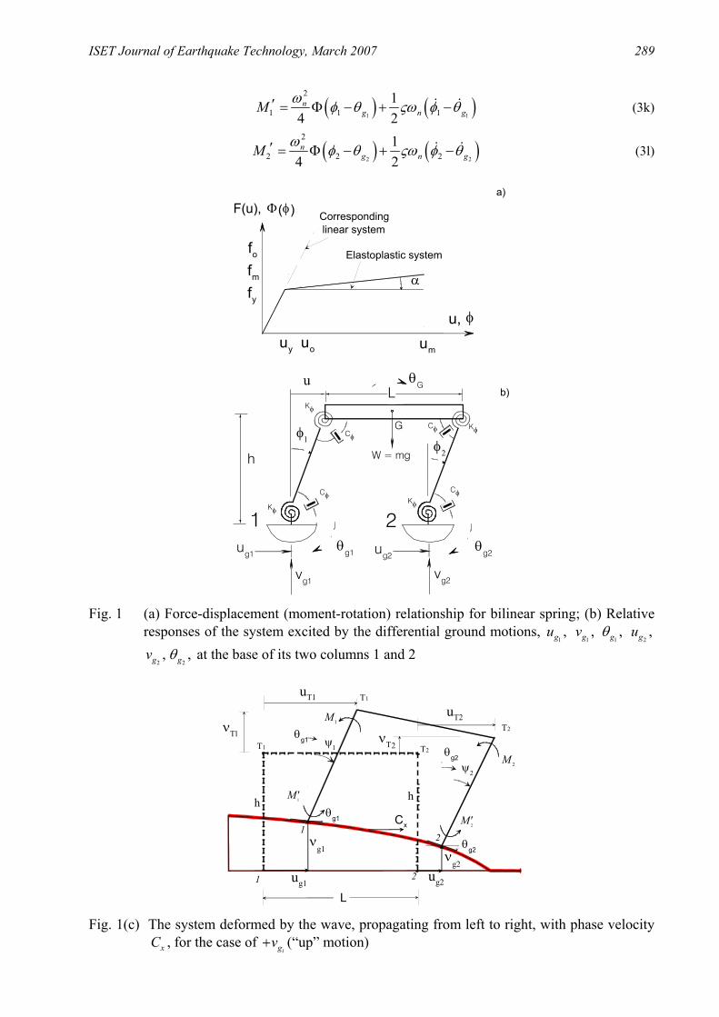
The nature of relative motion of individual column foundations or of the entire foundation system depends on the type of foundation, the characteristics of the soil surrounding the foundation, the type of incident waves, and on the direction of wave arrival, such that at the base of each column the motion has six degrees of freedom. In this paper we consider only the in-plane horizontal, vertical, and rocking components of the motion of column foundations, and the analysis will be performed for the structures on isolated foundations only. We assume that the structure is near the fault and that the longitudinal axis of the structure (X axis) coincides with the radial direction (r axis) of the propagation of waves from the earthquake source so that the displacements at the base of columns are different as a result of the wave passage. We suppose that excitations at the piers have the same amplitude with different phases. The phase difference (or time delay) will depend upon the distance between piers and the horizontal phase velocity of the incident waves. The simple model we consider is described in Figures 1(a), 1(b), and 1(c). It represents a one-story structure consisting of a rigid mass m with length L and supported by two rigid massless columns with height h, which are connected at the top to the mass and at the bottom to the ground by rotational springs (see Figure 1(b)). The stiffness of the springs, kφ , is assumed to be elastic-plastic, as shown in Figure 1(a), without hardening. The massless columns are connected to the ground and to the rigid mass by rotational dashpots, cφ , providing a fraction of critical damping equal to 5 percent. Rotation of the columns, ,iφ i = 1, 2, which is assumed not to be small, leads us to consider the geometric nonlinearity. The mass is acted upon by the acceleration due to gravity, g, and is excited by the differential horizontal, vertical, and rocking ground motions, ,

igu ,igv and ,

igθ i = 1, 2 (see Figure 1c) at the two bases such that

2 1 2 1 2 1( ) ( ) ; ( ) ( ) ; ( ) ( ) ;g g g g g g xu t u t v t v t t t L Cτ τ θ θ τ τ= − = − = − = (1)

with τ being the time delay between the motions at the two piers and xC being the horizontal phase velocity of the incident waves. The functional forms of ,

igu ,igv and

igθ are defined by the near-source

ground motions Fd and Nd , which are described in the next section. The governing differential equation for the system in Figures 1(b) and 1(c) is then

{ } { }2 1 2 1

1 11

2 2 2 2

2 2 22 1 2 1

( cos sin ) ( ) 0( cos sin ) ( cos sin )

sin sin (1 cos ) (1 cos ) 0g g g g

B C EA D t F DB C B C

L u h u h v h v h L

φ φ φφ φ φ φ

φ φ φ φ

−+ + − = − −

+ + − − + − − − + − − =

(2)

where

1 2 1 21 (1 cos ) (1 cos )sin g g

G

v v h hL

φ φθ − − − − + −

=

(3a)

1 2 1 1 2 2sin sincos

g gG

G

v v h hL

φ φ φ φθ

θ− − +

= (3b)


1 1 2 11 1

1 2 1 2

sin cos sin( )1 1 sin cos( ) 12 4 12cos cos cos cos sin sin( )2

GG

G G

A φ φ φ φφ φ θθ θ φ φ θ φ φ

−

= − + − − + + +

(3c)

2 12 1sin sing gL u u

Bh

φ φ+ −

= + − (3d)

2 12 1cos cosg gv v

Ch

φ φ−

= + − (3e)

2 1

2 1 2 12 1

1 2 1 2

1 cos( )2

sin cos sin( )1 sin cos( ) 14 12cos cos cos cos sin sin( )2

GG

G G

D φ φ

φ φ φ φφ φ θθ θ φ φ θ φ φ

= − −

−

+ − − − + +

(3f)

2 1 2 1

2 1 2 1

2 2

1 1 2 2 1 1 2 2

2 2 2 21 1 2 2 1 1 2 2

cos cos sin sin

sin sin cos cos

g g g g

g g g g

u u v vE

h h

u u v vB C

h h

φ φ φ φ φ φ φ φ

φ φ φ φ φ φ φ φ

− − = − + + + −

− −

+ + − + + −

(3g)

2 1 2 1

1

2 2 2 21 1 1 2 2 1 1 2 2

1 2 11

1 2 1 2

1

1 1cos sin sin cos cos2 2

cos( )sin( )1sin 12 cos cos cos sin sin( )2

cos112 cos

g g g g

G

G G

g g

G

u u v vgFh h h

v vL hh L

φ φ φ φ φ φ φ φ φ

φ θ φ φφθ φ φ θ φ φ

φθ

+ + = − − − + + − −

− −

× + + +

−− 2 2 2 2

1 1 2 2

2 1

1 2 1 2

11 2 1 2 2 1 1

2

2 1

1 2

cos cos sin

sin( )1cos cos cos sin sin( )2

cos( ) cos sin ( ) ( )2 cos

sin( )1cos cos cos si2

G G

G G

G

G

h

LM M M M M Mh

hL

φ φ φ φ θ θ

φ φ

θ φ φ θ φ φ

φφ θφ

φ φ

θ φ φ

− + +

−

× + +

′ ′+ + + + − +

−×

+( ) 1

2 2 1 12

1 2

coscosn sin( )G

M M M Mφφθ φ φ

′ ′− + − − +

(3h)

( ) ( )2

1 1 11

4 2n

G n GM ω φ θ ςω φ θ= Φ − + − (3i)

( ) ( )2

2 2 21

4 2n

G n GM ω φ θ ςω φ θ= Φ − + − (3j)


( ) ( )1 1

2

1 1 11

4 2n

g n gM ω φ θ ςω φ θ′ = Φ − + − (3k)

( ) ( )2 2

2

2 2 21

4 2n

g n gM ω φ θ ςω φ θ′ = Φ − + − (3l)

h

KφKφ

Kφ

Kφ

Cφ

ug1

u

G

L

W = mg

φ1

a)

b)

uo umuy

fo

fy

u, φ

Corresponding linear system

Elastoplastic system

αfm

F(u), Φ(φ)

ug2

Cφ

CφCφ

φ2

1 2θ

g2θ

g1

vg1vg2

θG

Fig. 1 (a) Force-displacement (moment-rotation) relationship for bilinear spring; (b) Relative

responses of the system excited by the differential ground motions, 1,gu

1,gv

1,gθ

2,gu

2 2, ,g gv θ at the base of its two columns 1 and 2

θg1

L

Cx

ug1

h h

1

T1

T1

T2

T2

2

uT2

νg1

12 θg2

θg1

θg2

ψ1

ψ2

νg2

ug2

νΤ2

νΤ1

uT1

1M

2M

1M ′

2M ′

Fig. 1(c) The system deformed by the wave, propagating from left to right, with phase velocity

xC , for the case of igv+ (“up” motion)


In Equation (3), when 0τ = , nω and ς are the circular natural frequency and damping ratio of the equivalent SDOF system, and ( )φΦ is a nonlinear function of the type described in Figure 1(a). For

0,τ ≠ the mass with length L has three degrees of freedom (horizontal and vertical translations of ,G and rotation ;Gθ see Figures 1(b) and 1(c)).

NEAR-SOURCE GROUND MOTION

In general, it is not possible to predict the detailed nature of the near-source ground motion and of the associated pulses due to irregular distribution of fault slip and because of non-uniform distribution of geologic rigidities surrounding the fault, non-uniform distribution of stress on the fault, and complex nonlinear processes that accompany the faulting (e.g., Trifunac, 1974; Trifunac and Udwadia, 1974; Mavroeidis et al., 2004). Thus, in this paper we adopt a simplified approach and model these motions using smooth pulses that have correct average amplitudes and durations and that have been compared to and calibrated against the observed fault slip and the recorded strong motions in terms of their peak amplitudes in time and their spectral content (Trifunac, 1993; Trifunac and Todorovska, 1994).

0 10 20Time - s

0

10

20

0 2 4 60

2

4

Dis

plac

emen

t - m

Fault

dN(t) dF(t)

dF(t)

dN(t)

2dN(t)

Dis

plac

emen

t - m

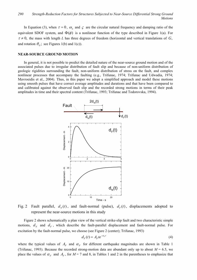
Fig. 2 Fault parallel, ( )Nd t , and fault-normal (pulse), ( )Fd t , displacements adopted to

represent the near-source motions in this study

Figure 2 shows schematically a plan view of the vertical strike-slip fault and two characteristic simple motions, Nd and Fd , which describe the fault-parallel displacement and fault-normal pulse. For excitation by the fault-normal pulse, we choose (see Figure 2 (center); Trifunac, 1993)

( ) FtF Fd t A te α−= (4)

where the typical values of FA and Fα for different earthquake magnitudes are shown in Table 1 (Trifunac, 1993). Because the recorded strong-motion data are abundant only up to about M = 6.5, we place the values of Fα and FA , for M = 7 and 8, in Tables 1 and 2 in the parentheses to emphasize that


these are based on extrapolation. For the near-source permanent displacement, we consider (see Figure 2 (bottom))

( ) 12

N

tN

NAd t e τ

− = −

(5)

The values of NA and Nτ for different earthquake magnitudes are shown in Table 2 (Trifunac, 1993).

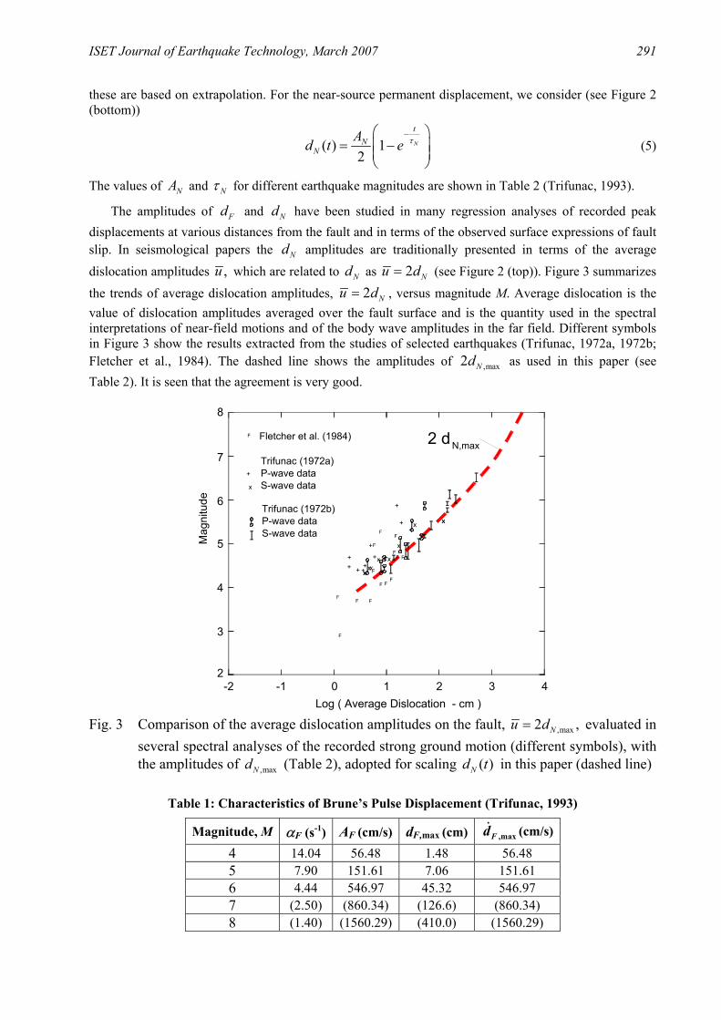
The amplitudes of Fd and Nd have been studied in many regression analyses of recorded peak displacements at various distances from the fault and in terms of the observed surface expressions of fault slip. In seismological papers the Nd amplitudes are traditionally presented in terms of the average dislocation amplitudes ,u which are related to Nd as 2 Nu d= (see Figure 2 (top)). Figure 3 summarizes the trends of average dislocation amplitudes, 2 Nu d= , versus magnitude M. Average dislocation is the value of dislocation amplitudes averaged over the fault surface and is the quantity used in the spectral interpretations of near-field motions and of the body wave amplitudes in the far field. Different symbols in Figure 3 show the results extracted from the studies of selected earthquakes (Trifunac, 1972a, 1972b; Fletcher et al., 1984). The dashed line shows the amplitudes of ,max2 Nd as used in this paper (see Table 2). It is seen that the agreement is very good.

-2 -1 0 1 2 3 4Log ( Average Dislocation - cm )

2

3

4

5Mag

nitu

de

8

7

6

2 dN,max

xx

x

xxxx

xx

x

x

+

++++

+

++

+

+

F

F

FF

FFF

FFF

F

FFF

F

Fletcher et al. (1984)

Trifunac (1972a)P-wave dataS-wave data

Trifunac (1972b)P-wave dataS-wave data

+

Fig. 3 Comparison of the average dislocation amplitudes on the fault, ,max2 ,Nu d= evaluated in

several spectral analyses of the recorded strong ground motion (different symbols), with the amplitudes of ,maxNd (Table 2), adopted for scaling ( )Nd t in this paper (dashed line)

Table 1: Characteristics of Brune’s Pulse Displacement (Trifunac, 1993)

Magnitude, M αF (s-1) AF (cm/s) dF,max (cm) ,maxFd (cm/s) 4 14.04 56.48 1.48 56.48 5 7.90 151.61 7.06 151.61 6 4.44 546.97 45.32 546.97 7 (2.50) (860.34) (126.6) (860.34) 8 (1.40) (1560.29) (410.0) (1560.29)


Table 2: Characteristics of Brune’s Near-Field Displacement (Trifunac, 1993)

Magnitude, M Nτ (s) NA (cm) ,maxNd (cm) ,maxNd (cm/s) 4 0.55 4.9 2.45 4.45 5 1.2 29.2 14.6 12.17 6 1.8 245.5 122.75 68.19 7 (3.0) (1288.0) (644.0) (214.7) 8 (5.0) (4169.0) (2084.5) (416.9)

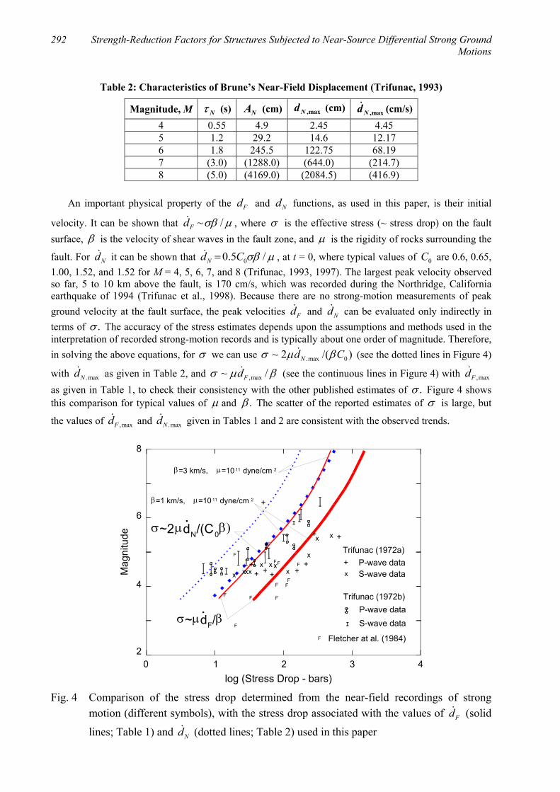
An important physical property of the Fd and Nd functions, as used in this paper, is their initial

velocity. It can be shown that ~ /Fd σβ µ , where σ is the effective stress (~ stress drop) on the fault surface, β is the velocity of shear waves in the fault zone, and µ is the rigidity of rocks surrounding the

fault. For Nd it can be shown that 00.5 /Nd C σβ µ= , at t = 0, where typical values of 0C are 0.6, 0.65, 1.00, 1.52, and 1.52 for M = 4, 5, 6, 7, and 8 (Trifunac, 1993, 1997). The largest peak velocity observed so far, 5 to 10 km above the fault, is 170 cm/s, which was recorded during the Northridge, California earthquake of 1994 (Trifunac et al., 1998). Because there are no strong-motion measurements of peak ground velocity at the fault surface, the peak velocities Fd and Nd can be evaluated only indirectly in terms of .σ The accuracy of the stress estimates depends upon the assumptions and methods used in the interpretation of recorded strong-motion records and is typically about one order of magnitude. Therefore, in solving the above equations, for σ we can use .max 0~ 2 /( )Nd Cσ µ β (see the dotted lines in Figure 4)

with .maxNd as given in Table 2, and ,max~ /Fdσ µ β (see the continuous lines in Figure 4) with ,maxFd as given in Table 1, to check their consistency with the other published estimates of .σ Figure 4 shows this comparison for typical values of µ and .β The scatter of the reported estimates of σ is large, but

the values of ,maxFd and .maxNd given in Tables 1 and 2 are consistent with the observed trends.

0 1 2 3 42

4

6

8

log (Stress Drop - bars)

Mag

nitu

de

Trifunac (1972a)P-wave data

S-wave data

Trifunac (1972b)P-wave data

S-wave data

Fletcher at al. (1984)

β=3 km/s, µ=10 11 dyne/cm 2

β=1 km/s, µ=10 11 dyne/cm 2 +

+

+

+

++ +++

F

F F

F F

F

F

F F

F

F

F

xx

x

xxxx

xxxx

+x

F

σ~µdF/β

.σ~2µdN/(C0

β)

.

Fig. 4 Comparison of the stress drop determined from the near-field recordings of strong

motion (different symbols), with the stress drop associated with the values of Fd (solid

lines; Table 1) and Nd (dotted lines; Table 2) used in this paper


Amplitudes of the pseudo relative velocity (PSV) spectra of the linear response of the SDOF systems in the far-field can be viewed and scaled in three period ranges, where the PSV amplitudes are dominated by (1) peak ground acceleration (for short periods), (2) peak ground velocity (for intermediate periods), and (3) peak ground displacement (for long periods) (Veletsos et al., 1965). When the fault motions Fd

and Nd begin with a sudden jump in the ground velocity (caused by a sudden stress drop on the fault surface), this large initial velocity will dominate the spectral amplitudes, and for the short periods of the oscillator, the “acceleration-dominated” zone of the PSV amplitudes will disappear. This will result in essentially constant PSV amplitudes in the short-period range (Jalali et al., 2007). This effect of large initial velocities, Fd and Nd , on the PSV spectral amplitudes in the short-period range is reminiscent of the effects of differential motions, particularly for the stiff structures, at soft soil sites, and for large plan dimensions. There, the peak strains in the soil (that are proportional to the peak ground velocity) lead to constant PSV spectral amplitudes at short periods (Trifunac and Todorovska, 1997; Trifunac and Gicev, 2006).

The presence of the motions resembling Nd in the recorded velocities and displacements filtered by data processing can be noticed by a trained eye in numerous plots of processed strong-motion records. The frequency of the occurrence and the amplitudes of such pulses are larger for the motions recorded closer to the causative faults. For the assumed motions Fd and Nd in this paper there is a Dirac delta function for the accelerations at time zero. In the observed motions, because of wave propagation through the sediments and soil, this will correspond to large but not infinite accelerations. Figure 5 (top) shows an example of the ground displacement, perpendicular to the fault, recorded during the Parkfield, California earthquake of 1966, about 3 km above and about 10 km south-east from the principal fault slip (Trifunac and Udwadia, 1974). This displacement, computed by double integration from the recorded and band-pass filtered accelerogram, is used here to illustrate an example of a near-field (not near-fault) “pulse-like” ground motion, which may have left the fault surface as Fd (shown in Figure 2 (middle)), but was subsequently attenuated and “filtered” along its 11 km long path between the south-eastern end of the fault slip and the recording station. Figure 5 (bottom) shows the ground displacement recorded several kilometers above the fault, which slipped during the San Fernando, California earthquake of 1971. This displacement was also band-pass filtered by the routine data processing methods, and therefore does not contain periods of motion longer than 15 s and shorter than 0.04 s. However, in spite of the band-pass filtering, it suggests two episodes of permanent ground displacements, starting near 2.5 and 6 s. Further examples of how Nd for this earthquake may have appeared in the near-field can be found in Figures 6 and 10 of Trifunac (1974), which are based on synthetic computation of the fault slip during the San Fernando earthquake of 1971. The displacements shown in Figure 5 are examples of the recorded near-field (but not near-fault, or fault) motions, which lend support to our choice of the simple fault displacement functions, Fd and Nd .

The functions Fd and Nd model the displacement time histories in the fault-normal and fault-

parallel directions. For the vertical strike-slip faults, Fd and Nd will also represent strike-normal and strike-parallel motions along the surface expression of the fault. For the dip-slip faults, a linear combination of Fd and Nd will contribute only to the vertical and strike-normal displacements on the

ground surface. For a general fault orientation both Fd and Nd will contribute to the surface displacements, as determined by their projections onto horizontal and vertical motions on the ground surface (Mavroeidis and Papageorgiou, 2003). In the following, we will refer to Fd and Nd in the context of vertical strike-slip faults only. In this paper, for simplicity, we assume that ( ) ( )

i ig gv t u t= ± and that the functional form of ( )igu t is

defined by Equations (4) and (5) for the fault-normal pulse and fault-parallel displacement, respectively. In the following plots, we label the results for

igv+ with “up”, and those for igv− with “down”. The

rocking component of the ground motion will be approximated by (Trifunac, 1982; Lee and Trifunac, 1987)


1( ) ( )

i ig gx

t v tC

θ

= −

(6)

where ( )igv t is the vertical velocity of the ground motion at the ith column. Of course, in a more accurate

modeling, the ratio of igv to

igu amplitudes will depend on the incident angle and the character of

incident waves, while the associated rocking igθ will be described by a superposition of rocking angles

associated with the incident body and dispersed surface waves (Lee and Trifunac, 1987). The sensitivity studies of how the strength-reduction factors will depend on different incident angles is beyond the scope of this paper, and will be addressed in our future work.

STATION NO. 2, CALIFORNIA COMP N65EPARKFIELD EARTHQUAKE JUNE 27, 1966

Time (s)10

Dis

plac

emen

t (c

m)

PACOIMA DAM, CALIFORNIA COMP S15WSAN FERNANDO EARTHQUAKE FEB 9, 1971

5

40

150-40

0

Time (s)105 150

20

-20

0

Dis

plac

emen

t (c

m)

Fig. 5 Ground displacement, perpendicular to the fault strike, about 10 km south-east and 3 km

above the south-eastern end of the fault slip on a vertical strike-slip fault, during the Parkfield, California, earthquake of 1966 (Trifunac and Udwadia, 1974) (top); Ground displacement recorded near the center and several kilometers above the thrust fault, which ruptured during the San Fernando, California, earthquake of 1971 (bottom)

STRENGTH-REDUCTION FACTORS OF THE SYSTEM UNDER DIFFERENTIAL GROUND MOTIONS

The yield-strength reduction factor for the system subjected to a synchronous ground motion is yR =

0 0/ / ,y yf f u u= where all of the quantities are defined as in Figure 1(a). In this paper, for the assumed model and because of the differential ground motions and rotation of the beam, relative rotation for the two columns at their top and bottom will be different. Therefore, we define the R-factor and ductility for each corner of the system instead of one factor for the whole system: at the top of the left column,

10 1; Gtl tl

y y

MRM

φ θµφ−

= = (7)

at the bottom of the left column,

1

10 11 1; ;bl bl g

y y

MRM

ψµ ψ φ θφ

′= = = − (8)

at the top of the right column,


20 2; Gtr tr

y y

MRM

φ θµφ−

= = (9)

and at the bottom of the right column,

2

20 22 2; ;br br g

y y

MRM

ψµ ψ φ θφ

′= = = − (10)

In Equations (7)–(10), 10 ,M 10 ,M ′ 20 ,M and 20M ′ are the maximum linear moments, and 1( ),Gφ θ−

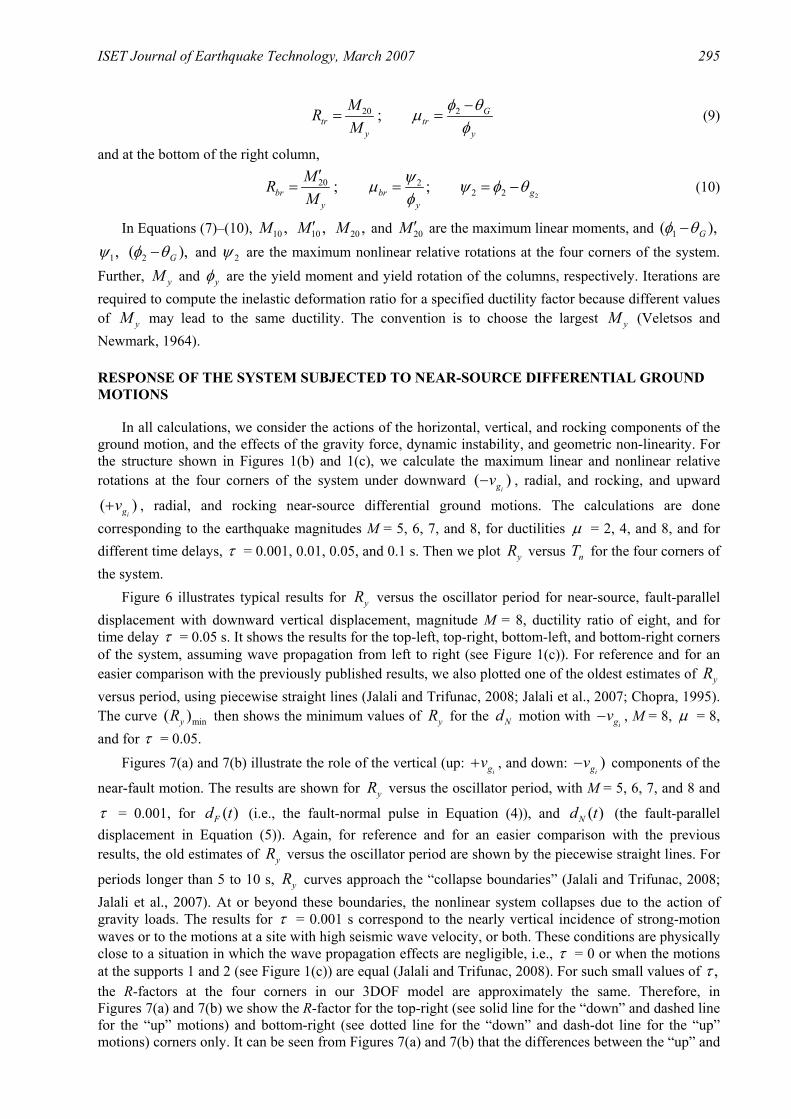
1,ψ 2( ),Gφ θ− and 2ψ are the maximum nonlinear relative rotations at the four corners of the system. Further, yM and yφ are the yield moment and yield rotation of the columns, respectively. Iterations are required to compute the inelastic deformation ratio for a specified ductility factor because different values of yM may lead to the same ductility. The convention is to choose the largest yM (Veletsos and Newmark, 1964).

RESPONSE OF THE SYSTEM SUBJECTED TO NEAR-SOURCE DIFFERENTIAL GROUND MOTIONS

In all calculations, we consider the actions of the horizontal, vertical, and rocking components of the ground motion, and the effects of the gravity force, dynamic instability, and geometric non-linearity. For the structure shown in Figures 1(b) and 1(c), we calculate the maximum linear and nonlinear relative rotations at the four corners of the system under downward ( )

igv− , radial, and rocking, and upward

( )igv+ , radial, and rocking near-source differential ground motions. The calculations are done

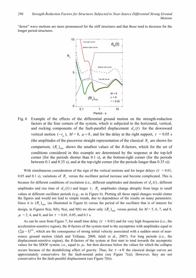
corresponding to the earthquake magnitudes M = 5, 6, 7, and 8, for ductilities µ = 2, 4, and 8, and for different time delays, τ = 0.001, 0.01, 0.05, and 0.1 s. Then we plot yR versus nT for the four corners of the system. Figure 6 illustrates typical results for yR versus the oscillator period for near-source, fault-parallel displacement with downward vertical displacement, magnitude M = 8, ductility ratio of eight, and for time delay τ = 0.05 s. It shows the results for the top-left, top-right, bottom-left, and bottom-right corners of the system, assuming wave propagation from left to right (see Figure 1(c)). For reference and for an easier comparison with the previously published results, we also plotted one of the oldest estimates of yR versus period, using piecewise straight lines (Jalali and Trifunac, 2008; Jalali et al., 2007; Chopra, 1995). The curve min( )yR then shows the minimum values of yR for the Nd motion with

igv− , M = 8, µ = 8, and for τ = 0.05.

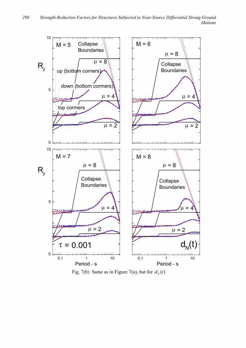
Figures 7(a) and 7(b) illustrate the role of the vertical (up: igv+ , and down: )

igv− components of the

near-fault motion. The results are shown for yR versus the oscillator period, with M = 5, 6, 7, and 8 and

τ = 0.001, for ( )Fd t (i.e., the fault-normal pulse in Equation (4)), and ( )Nd t (the fault-parallel displacement in Equation (5)). Again, for reference and for an easier comparison with the previous results, the old estimates of yR versus the oscillator period are shown by the piecewise straight lines. For

periods longer than 5 to 10 s, yR curves approach the “collapse boundaries” (Jalali and Trifunac, 2008; Jalali et al., 2007). At or beyond these boundaries, the nonlinear system collapses due to the action of gravity loads. The results for τ = 0.001 s correspond to the nearly vertical incidence of strong-motion waves or to the motions at a site with high seismic wave velocity, or both. These conditions are physically close to a situation in which the wave propagation effects are negligible, i.e., τ = 0 or when the motions at the supports 1 and 2 (see Figure 1(c)) are equal (Jalali and Trifunac, 2008). For such small values of ,τ the R-factors at the four corners in our 3DOF model are approximately the same. Therefore, in Figures 7(a) and 7(b) we show the R-factor for the top-right (see solid line for the “down” and dashed line for the “up” motions) and bottom-right (see dotted line for the “down” and dash-dot line for the “up” motions) corners only. It can be seen from Figures 7(a) and 7(b) that the differences between the “up” and


“down” wave motions are more pronounced for the stiff structures and that those tend to decrease for the longer period structures.

Bottom-left corner

Bottom-right corner

Top-left corner

Top-right corner

0

10

5

Ry

0.1 1 10Period - s

M = 8µ = 8τ = 0.05

dN(t)

(Ry)min

Fig. 6 Example of the effects of the differential ground motion on the strength-reduction

factors at the four corners of the system, which is subjected to the horizontal, vertical, and rocking components of the fault-parallel displacement ( )Nd t for the downward vertical motion ( ),

igv− M = 8, 8µ = , and for the delay at the right support, τ = 0.05 s (the amplitudes of the piecewise straight representation of the classical yR are shown for comparison; min( )yR shows the smallest values of the R-factors, which for the set of conditions considered in this example are determined by the response at the top-left corner (for the periods shorter than 0.1 s), at the bottom-right corner (for the periods between 0.1 and 0.35 s), and at the top-right corner (for the periods longer than 0.35 s))

With simultaneous consideration of the sign of the vertical motions and for larger delays (τ = 0.01, 0.05 and 0.1 s), variations of yR versus the oscillator period increase and become complicated. This is

because for different conditions of excitation (i.e., different amplitudes and durations of ( )Fd t , different amplitudes and rise time of ( )Nd t ) and larger ,τ yR amplitudes change abruptly from large to small values at different oscillator periods (e.g., as in Figure 6). Plotting all those rapid changes would clutter the figures and would not lead to simple trends, due to dependence of the results on many parameters. Since it is min( )yR (as illustrated in Figure 6) versus the period of the oscillator that is of interest for

design, in Figures 8(a), 8(b), 9(a), and 9(b) we show only min( )yR versus period, for M = 5, 6, 7, and 8, µ = 2, 4, and 8, and for τ = 0.01, 0.05, and 0.1 s.

As can be seen from Figure 7, for small time delay (τ = 0.01) and for very high frequencies (i.e., the acceleration-sensitive region), the R-factors of the system tend to the asymptotes with amplitudes equal to

1 2(2 1)µ − , which are the consequence of strong initial velocity associated with a sudden onset of near-source ground motion (Jalali and Trifunac, 2008; Jalali et al., 2007). For long periods (i.e., the displacement-sensitive region), the R-factors of the system at first start to tend towards the asymptotic values for the SDOF system, i.e., equal to ,µ but then decrease below the values for which the collapse occurs because of the destabilizing effect of gravity. Thus, for 0τ → the classical design curves are approximately conservative for the fault-normal pulse (see Figure 7(a)). However, they are not conservative for the fault-parallel displacement (see Figure 7(b)).


0.1 1 10Period - s

0

10

5

0

10

5

Ry

Ry

M = 8

µ = 8

0.1 1 10Period - s

M = 7

M = 6

CollapseBoundaries

CollapseBoundary

µ = 8

µ = 4

µ = 2

µ = 4

µ = 2

µ = 8 µ = 8

µ = 4µ = 4

µ = 2 µ = 2

τ = 0.001 dF(t)

up (bottom corners)down (bottom corners)

down (top corners)

up (top corners)

M = 5

Fig. 7(a) An example of the effects of the differential ground motions on the strength-reduction

factors at the corners of the system shown in Figure 1(b), which is subjected to the horizontal, vertical, and rocking components of the fault-normal pulse ( ),Fd t for the “down” (

igv− ) and “up” (igv+ ) vertical components, M = 5, 6, 7, and 8, µ = 2, 4, and

8, and for the delay time τ = 0.001 s (for this ,τ the R-factors for the left and right columns are approximately same)


0.1 1 10Period - s

0

10

5

0

10

5

Ry

Ry

M = 8

µ = 8

0.1 1 10Period - s

M = 7

M = 6M = 5

CollapseBoundaries

CollapseBoundaries

CollapseBoundaries

CollapseBoundaries

µ = 8

µ = 4µ = 4

µ = 2µ = 2

µ = 8 µ = 8

µ = 4µ = 4

µ = 2 µ = 2

dN(t)τ = 0.001

up (bottom corners)

down (bottom cormers)

top cormers

Fig. 7(b) Same as in Figure 7(a), but for ( )Nd t


0.1 1 10 0.1 1 100.1 1 100

10

5

0

10

5

(Ry)min

M = 6

M = 5

µ = 2

µ = 2 µ = 4 µ = 8

µ = 8µ = 4

Period - s

(Ry)min

(2µ - 1) 1/2

(2µ - 1) 1/2

(2µ - 1) 1/2

(2µ - 1) 1/2

(2µ - 1) 1/2

(2µ - 1) 1/2

τ = 0.01

τ = 0.05τ = 0.1

τ = 0.01

τ = 0.05

τ = 0.1

dF(t)

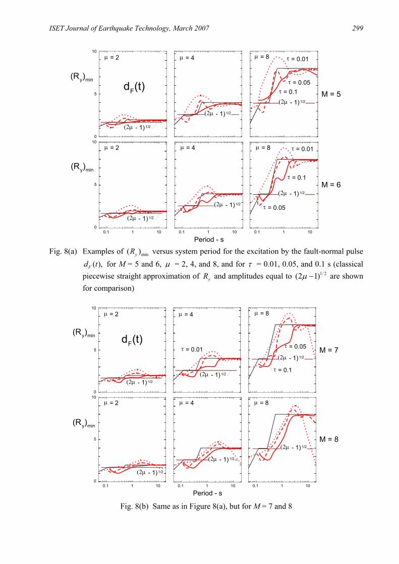
Fig. 8(a) Examples of min( )yR versus system period for the excitation by the fault-normal pulse

( ),Fd t for M = 5 and 6, µ = 2, 4, and 8, and for τ = 0.01, 0.05, and 0.1 s (classical piecewise straight approximation of yR and amplitudes equal to 1/ 2(2 1)µ − are shown for comparison)

0.1 1 10 0.1 1 100.1 1 100

10

5

0

10

5

M = 8

M = 7

µ = 2

µ = 2 µ = 4 µ = 8

µ = 8µ = 4

Period - s

τ = 0.01 τ = 0.05

τ = 0.1

(2µ - 1) 1/2

(2µ - 1) 1/2

(2µ - 1) 1/2

(2µ - 1) 1/2

(2µ - 1) 1/2

(2µ - 1) 1/2

(Ry)min

(Ry)min

dF(t)

Fig. 8(b) Same as in Figure 8(a), but for M = 7 and 8


0.1 1 10 0.1 1 100.1 1 100

10

5

0

10

5

M = 6

M = 5

µ = 2

µ = 2 µ = 4 µ = 8

µ = 8µ = 4

Period - s

(Ry)min

(Ry)min

(2µ - 1) 1/2

(2µ - 1) 1/2

(2µ - 1) 1/2

(2µ - 1) 1/2

(2µ - 1) 1/2

(2µ - 1) 1/2

τ = 0.01τ = 0.05

τ = 0.1

dN(t)

Fig. 9(a) Same as in Figure 8(a), but for ( )Nd t

0.1 1 10 0.1 1 100.1 1 100

10

5

0

10

5

M = 8

M = 7

µ = 2

µ = 2 µ = 4 µ = 8

µ = 8µ = 4

Period - s

(Ry)min

(Ry)min

(2µ - 1) 1/2

(2µ - 1) 1/2

(2µ - 1) 1/2

(2µ - 1) 1/2

(2µ - 1) 1/2 (2µ - 1) 1/2

τ = 0.01

τ = 0.1τ = 0.05

dN(t)

Fig. 9(b) Same as in Figure 9(a), but for M = 7 and 8

With increasing time delay, the R-factors at the four corners of the system become very different. From Figures 8(a), 8(b), 9(a), and 9(b), it can be seen that for the fault-normal pulse with increasing time delay, the R-factors of the system fall below the classical design curves for the periods between 0.1 and 2.0 s. For the fault-parallel displacement with increasing time delay, the R-factors of the system fall even


below the value of 1 2(2 1)µ − by 30 to 50 percent for most periods, and for the cases studied in this paper, mainly for the periods between 0.1 and 2.0 s.

CONCLUSIONS

We have illustrated the effects of differential motion on the strength-reduction factors, yR versus ,nT for a simple 3DOF system subjected to propagating horizontal, vertical, and rocking components of near-source ground motions. For small time delays and for very-high-frequency systems, the R-factors are dominated by the initial velocity of the ground motion and those tend to the amplitudes equal to

1 2(2 1)µ − (Jalali and Trifunac, 2008; Jalali et al., 2007). For τ = 0, the classical design curves are approximately conservative for the fault-normal pulse, but they are not conservative for the fault-parallel displacement. With increasing time delay (in this paper we studied delays up to 0.1 s), the R-factors at the four corners of our model (see Figure 1(b)) become different and move below the classical design curves for the periods between 0.1 and 2.0 s for the fault-normal pulse, and essentially for all the periods for the fault-parallel displacements. In view of these results, it is recommended that for design in the near-field, i.e., close to active faults, the strength-reduction factors for all the components of strong motion should be constant and equal to

1 2(2 1)µ − for long periods, but only up to the collapse boundaries where dynamic instability and gravity effects become dominant. For the periods shorter than about 2 s, these strength-reduction factors should be further reduced by 30 to 50 percent.

REFERENCES

1. ATC (1996). “Seismic Evaluation and Retrofit of Concrete Buildings: Volume 1”, Report ATC-40, Applied Technology Council, Redwood City, California, U.S.A.

2. Baez, J.I. and Miranda, E. (2000). “Amplification Factors to Estimate Inelastic Displacement Demands for the Design of Structures in the Near Field”, Proceedings of the 12th World Conference on Earthquake Engineering, Auckland, New Zealand, Paper No. 1561 (on CD).

3. Biot, M.A. (1932). “Transient Oscillations in Elastic Systems”, Ph.D. Thesis No. 259, Aeronautics Department, California Institute of Technology, Pasadena, U.S.A.

4. Biot, M.A. (1933). “Theory of Elastic Systems Vibrating under Transient Impulse with an Application to Earthquake-Proof Buildings”, Proceedings of the National Academy of Sciences of the United States of America, Vol. 19, No. 2, pp. 262–268.

5. Biot, M.A. (1934). “Theory of Vibration of Buildings during Earthquake”, Zeitschrift für Angewandte Matematik und Mechanik, Vol. 14, No. 4, pp. 213–223.

6. Bogdanoff, J.L., Goldberg, J.E. and Schiff, A.J. (1965). “The Effect of Ground Transmission Time on the Response of Long Structures”, Bulletin of the Seismological Society of America, Vol. 55, No. 3, pp. 627–640.

7. Chakraborti, A. and Gupta, V.K. (2005). “Scaling of Strength Reduction Factors for Degrading Elasto-Plastic Oscillators”, Earthquake Engineering & Structural Dynamics, Vol. 34, No. 2, pp. 189–206.

8. Chopra, A.K. (1995). “Dynamics of Structures: Theory and Applications to Earthquake Engineering”, Prentice-Hall, Englewood Cliffs, U.S.A.

9. Chopra, A.K. and Chintanapakdee, C. (2001). “Comparing Response of SDF Systems to Near-Fault and Far-Fault Earthquake Motions in the Context of Spectral Regions”, Earthquake Engineering & Structural Dynamics, Vol. 30, No. 12, pp. 1769–1789.

10. Chopra, A.K. and Chintanapakdee, C. (2004). “Inelastic Deformation Ratios for Design and Evaluation of Structures: Single-Degree-of-Freedom Bilinear Systems”, Journal of Structural Engineering, ASCE, Vol. 130, No. 9, pp. 1309–1319.

11. Cuesta, I. and Aschheim, M.A. (2001). “Isoductile Strengths and Strength Reduction Factors of Elasto-Plastic SDOF Systems Subjected to Simple Waveforms”, Earthquake Engineering & Structural Dynamics, Vol. 30, No. 7, pp. 1043–1059.


12. FEMA (1997a). “NEHRP Guidelines for the Seismic Rehabilitation of Buildings”, Report FEMA 273, Federal Emergency Management Agency, Washington, DC, U.S.A.

13. FEMA (1997b). “NEHRP Commentary on the Guidelines for the Seismic Rehabilitation of Buildings”, Report FEMA 274, Federal Emergency Management Agency, Washington, DC, U.S.A.

14. FEMA (2000). “Prestandard and Commentary for the Seismic Rehabilitation of Buildings”, Report FEMA 356, Federal Emergency Management Agency, Washington, DC, U.S.A.

15. Fletcher, J., Boatwright, J., Haar, L., Hanks, T. and McGarr, A. (1984). “Source Parameters for Aftershocks of the Oroville, California, Earthquake”, Bulletin of the Seismological Society of America, Vol. 74, No. 4, pp. 1101–1123.

16. Hao, H. (1989). “Effects of Spatial Variation of Ground Motions on Large Multiply-Supported Structures”, Report UCB/EERC-89/06, University of California, Berkeley, U.S.A.

17. Hao, H. (1991). “Response of Multiply Supported Rigid Plate to Spatially Correlated Seismic Excitations”, Earthquake Engineering & Structural Dynamics, Vol. 20, No. 9, pp. 821–838.

18. Harichandran, R.S. and Vanmarcke, E.H. (1986). “Stochastic Variation of Earthquake Ground Motion in Space and Time”, Journal of Engineering Mechanics, ASCE, Vol. 112, No. 2, pp. 154–174.

19. Harichandran, R.S. and Wang, W. (1988). “Response of Simple Beam to Spatially Varying Earthquake Excitation”, Journal of Engineering Mechanics, ASCE, Vol. 114, No. 9, pp. 1526–1541.

20. Harichandran, R.S. and Wang, W. (1990). “Response of Intermediate Two-Span Beam to Spatially Varying Seismic Excitation”, Earthquake Engineering & Structural Dynamics, Vol. 19, No. 2, pp. 173–187.

21. Hyun, C.H., Yun, C.B. and Lee, D.G. (1992). “Nonstationary Response Analysis of Suspension Bridges for Multiple Support Excitations”, Probabilistic Engineering Mechanics, Vol. 7, No. 1, pp. 27–35.

22. Jalali, R.S. and Trifunac, M.D. (2008). “A Note on Strength Reduction Factors for Design of Structures near Earthquake Faults”, Soil Dynamics and Earthquake Engineering, Vol. 28, No. 3 (in press).

23. Jalali, R.S., Trifunac, M.D., Ghodrati Amiri, G. and Zahedi, M. (2007). “Wave-Passage Effects on Strength-Reduction Factors for Design of Structures near Earthquake Faults”, Soil Dynamics and Earthquake Engineering, Vol. 27, No. 8, pp. 703–711.

24. Kashefi, I. and Trifunac, M.D. (1986). “Investigation of Earthquake Response of Simple Bridge Structures”, Report CE 86-02, University of Southern California, Los Angeles, U.S.A.

25. Kojic, S.B. and Trifunac, M.D. (1991a). “Earthquake Stresses in Arch Dams. I: Theory and Antiplane Excitation”, Journal of Engineering Mechanics, ASCE, Vol. 117, No. 3, pp. 532–552.

26. Kojic, S.B. and Trifunac, M.D. (1991b). “Earthquake Stresses in Arch Dams. II: Excitation by SV, P, and Rayleigh Waves”, Journal of Engineering Mechanics, ASCE, Vol. 117, No. 3, pp. 553–574.

27. Kojic, S.B., Trifunac, M.D. and Lee, V.W. (1988). “Earthquake Response of Arch Dams to Nonuniform Canyon Motion”, Report CE 88-03, University of Southern California, Los Angeles, U.S.A.

28. Lee, V.W. and Trifunac, M.D. (1987). “Rocking Strong Earthquake Accelerations”, Soil Dynamics and Earthquake Engineering, Vol. 6, No. 2, pp. 75–89.

29. Loh, C.H., Penzien, J. and Tsai, Y.B. (1982). “Engineering Analyses of SMART 1 Array Accelerograms”, Earthquake Engineering & Structural Dynamics, Vol. 10, No. 4, pp. 575–591.

30. MacRae, G.A., Morrow, D.V. and Roeder, C.W. (2001). “Near-Fault Ground Motion Effects on Simple Structures”, Journal of Structural Engineering, ASCE, Vol. 127, No. 9, pp. 996–1004.

31. Mavroeidis, G.P. and Papageorgiou, A.S. (2003). “A Mathematical Representation of Near-Fault Ground Motions”, Bulletin of the Seismological Society of America, Vol. 93, No. 3, pp. 1099–1131.

32. Mavroeidis, G.P., Dong, G. and Papageorgiou, A.S. (2004). “Near-Fault Ground Motions, and the Response of Elastic and Inelastic Single-Degree-of-Freedom (SDOF) Systems”, Earthquake Engineering & Structural Dynamics, Vol. 33, No. 9, pp. 1023–1049.

33. Miranda, E. (1991). “Seismic Evaluation and Upgrading of Existing Structures”, Ph.D. Dissertation, Department of Civil Engineering, University of California, Berkeley, U.S.A.


34. Miranda, E. (2000). “Inelastic Displacement Ratios for Structures on Firm Sites”, Journal of Structural Engineering, ASCE, Vol. 126, No. 10, pp. 1150–1159.

35. Mylonakis, G. and Voyagaki, E. (2006). “Yielding Oscillator Subjected to Simple Pulse Waveforms: Numerical Analysis & Closed-Form Solutions”, Earthquake Engineering & Structural Dynamics, Vol. 35, No. 15, pp. 1949–1974.

36. Okubo, T., Arakawa, T. and Kawashima, K. (1984). “Dense Instrument Array Program of the Public Works Research Institute and Preliminary Analysis of the Records”, Proceedings of the Eighth World Conference on Earthquake Engineering, San Francisco, U.S.A., Vol. II, pp. 151–158.

37. Perotti, F. (1990). “Structural Response to Non-stationary Multiple-Support Random Excitation”, Earthquake Engineering & Structural Dynamics, Vol. 19, No. 4, pp. 513–527.

38. Riddell, R. and Newmark, N.M. (1979). “Statistical Analysis of the Response of Nonlinear Systems Subjected to Earthquakes”, Structural Research Series 468, Department of Civil Engineering, University of Illinois at Urbana-Champaign, Urbana, U.S.A.

39. Riddell, R., Garcia, J.E. and Garces, E. (2002). “Inelastic Deformation Response of SDOF Systems Subjected to Earthquakes”, Earthquake Engineering & Structural Dynamics, Vol. 31, No. 3, pp. 515–538.

40. Ruiz-Garcia, J. and Miranda, E. (2003). “Inelastic Displacement Ratios for Evaluation of Existing Structures”, Earthquake Engineering & Structural Dynamics, Vol. 32, No. 8, pp. 1237–1258.

41. Ruiz-Garcia, J. and Miranda, E. (2006). “Inelastic Displacement Ratios for Evaluation of Structures Built on Soft Soil Sites”, Earthquake Engineering & Structural Dynamics, Vol. 35, No. 6, pp. 679–694.

42. Tiwari, A.K. and Gupta, V.K. (2000). “Scaling of Ductility and Damage-Based Strength Reduction Factors for Horizontal Motions”, Earthquake Engineering & Structural Dynamics, Vol. 29, No. 7, pp. 969–987.

43. Todorovska, M.I. and Lee, V.W. (1989). “Seismic Waves in Buildings with Shear Walls or Central Core”, Journal of Engineering Mechanics, ASCE, Vol. 115, No. 12, pp. 2669–2686.

44. Todorovska, M.I. and Trifunac, M.D. (1989). “Antiplane Earthquake Waves in Long Structures”, Journal of Engineering Mechanics, ASCE, Vol. 115, No. 12, pp. 2687–2708.

45. Todorovska, M.I. and Trifunac, M.D. (1990a). “A Note on the Propagation of Earthquake Waves in Buildings with Soft First Floor”, Journal of Engineering Mechanics, ASCE, Vol. 116, No. 4, pp. 892–900.

46. Todorovska, M.I. and Trifunac, M.D. (1990b). “Note on Excitation of Long Structures by Ground Waves”, Journal of Engineering Mechanics, ASCE, Vol. 116, No. 4, pp. 952–964.

47. Todorovska, M.I., Gupta, I.D., Gupta, V.K., Lee, V.W. and Trifunac, M.D. (1995). “Selected Topics in Probabilistic Seismic Hazard Analysis”, Report CE 95-08, University of Southern California, Los Angeles, U.S.A.

48. Trifunac, M.D. (1972a). “Stress Estimates for the San Fernando, California, Earthquake of February 9, 1971: Main Event and Thirteen Aftershocks”, Bulletin of the Seismological Society of America, Vol. 62, No. 3, pp. 721–750.

49. Trifunac, M.D. (1972b). “Tectonic Stress and the Source Mechanism of the Imperial Valley, California, Earthquake of 1940”, Bulletin of the Seismological Society of America, Vol. 62, No. 5, pp. 1283–1302.

50. Trifunac, M.D. (1974). “A Three-Dimensional Dislocation Model for the San Fernando, California, Earthquake of February 9, 1971”, Bulletin of the Seismological Society of America, Vol. 64, No. 1, pp. 149–172.

51. Trifunac, M.D. (1982). “A Note on Rotational Components of Earthquake Motions on Ground Surface for Incident Body Waves”, International Journal of Soil Dynamics and Earthquake Engineering, Vol. 1, No. 1, pp. 11–19.

52. Trifunac, M.D. (1993). “Broad Band Extension of Fourier Amplitude Spectra of Strong Motion Acceleration”, Report CE 93-01, University of Southern California, Los Angeles, U.S.A.

53. Trifunac, M.D. (1997). “Stresses and Intermediate Frequencies of Strong Earthquake Acceleration”, Geofizika, Vol. 14, pp. 1–27.


54. Trifunac, M.D. (2003). “23rd ISET Annual Lecture: 70-th Anniversary of Biot Spectrum”, ISET Journal of Earthquake Technology, Vol. 40, No. 1, pp. 19–50.

55. Trifunac, M.D. (2006). “Effects of Torsional and Rocking Excitations on the Response of Structures” in “Earthquake Source Asymmetry, Structural Media and Rotation Effects (edited by R. Teisseyre, M. Takeo and E. Majewski), Springer-Verlag, Heidelberg, Germany.

56. Trifunac, M.D. and Gicev, V. (2006). “Response Spectra for Differential Motion of Columns, Paper II: Out-of-Plane Response”, Soil Dynamics and Earthquake Engineering, Vol. 26, No. 12, pp. 1149–1160.

57. Trifunac, M.D. and Todorovska, M.I. (1994). “Broad Band Extension of Pseudo Relative Velocity Spectra of Strong Ground Motion”, Report CE 94-02, University of Southern California, Los Angeles, U.S.A.

58. Trifunac, M.D. and Todorovska, M.I. (1997). “Response Spectra for Differential Motion of Columns”, Earthquake Engineering & Structural Dynamics, Vol. 26, No. 2, pp. 251–268.

59. Trifunac, M.D. and Todorovska, M.I. (2001). “Evolution of Accelerographs, Data Processing, Strong Motion Arrays and Amplitude and Spatial Resolution in Recording Strong Earthquake Motion”, Soil Dynamics and Earthquake Engineering, Vol. 21, No. 6, pp. 537–555.

60. Trifunac, M.D. and Udwadia, F.E. (1974). “Parkfield, California, Earthquake of June 27, 1966: A Three-Dimensional Moving Dislocation”, Bulletin of the Seismological Society of America, Vol. 64, No. 3-1, pp. 511–533.

61. Trifunac, M.D., Todorovska, M.I. and Lee, V.W. (1998). “The Rinaldi Strong Motion Accelerogram of the Northridge, California, Earthquake of 17 January, 1994”, Earthquake Spectra, Vol. 14, No. 1, pp. 225–239.

62. Veletsos, A.S. and Newmark, N.M. (1960). “Effect of Inelastic Behavior on the Response of Simple Systems to Earthquake Motions”, Proceedings of the Second World Conference on Earthquake Engineering, Tokyo, Japan, Vol. II, pp. 859–912.

63. Veletsos, A.S. and Newmark, N.M. (1964). “Design Procedures for Shock Isolation Systems of Underground Protective Structures. Volume III. Response Spectra of Single-Degree-of-Freedom Elastic and Inelastic Systems”, Report RTD TDR 63-3096 (prepared for Air Force Weapons Laboratory, Kirtland Air Force Base, Albuquerque, New Mexico), Newmark Hansen and Associates, Urbana, U.S.A.

64. Veletsos, A.S. and Vann, W.P. (1971). “Response of Ground-Excited Elastoplastic Systems”, Journal of the Structural Division, Proceedings of ASCE, Vol. 97, No. ST4, pp. 1257–1281.

65. Veletsos, A.S., Newmark, N.M. and Celapati, C.V. (1965). “Deformation Spectra for Elastic and Elastoplastic Systems Subjected to Ground Shock and Earthquake Motion”, Proceedings of the Third World Conference on Earthquake Engineering, Wellington, New Zealand, Vol. II, pp. 663–682.

66. Zerva, A. (1991). “Effect of Spatial Variability and Propagation of Seismic Ground Motions on the Response of Multiply Supported Structures”, Probabilistic Engineering Mechanics, Vol. 6, No. 3-4, pp. 212–221.

67. Zembaty, Z. and Krenk, S. (1993). “Spatial Seismic Excitations and Response Spectra”, Journal of Engineering Mechanics, ASCE, Vol. 119, No. 12, pp. 2449–2460.

68. Zembaty, Z. and Krenk, S. (1994). “Response Spectra of Spatial Seismic Ground Motion”, Proceedings of the Tenth European Conference on Earthquake Engineering, Vienna, Austria, Vol. 2, pp. 1271–1275.

STRENGTH-REDUCTION FACTORS FOR STRUCTURES SUBJECTED …home.iitk.ac.in/~vinaykg/Iset486.pdf · 286...

Documents

Transcript of STRENGTH-REDUCTION FACTORS FOR STRUCTURES SUBJECTED …home.iitk.ac.in/~vinaykg/Iset486.pdf · 286...