
Streamline Simulation with Capillary Effects Applied to …orbit.dtu.dk/files/2496640/Roman A...
181
General rights Copyright and moral rights for the publications made accessible in the public portal are retained by the authors and/or other copyright owners and it is a condition of accessing publications that users recognise and abide by the legal requirements associated with these rights. • Users may download and print one copy of any publication from the public portal for the purpose of private study or research. • You may not further distribute the material or use it for any profit-making activity or commercial gain • You may freely distribute the URL identifying the publication in the public portal If you believe that this document breaches copyright please contact us providing details, and we will remove access to the work immediately and investigate your claim. Downloaded from orbit.dtu.dk on: Aug 10, 2018 Streamline Simulation with Capillary Effects Applied to Petroleum Engineering Problems Berenblyum, Roman; Stenby, Erling Halfdan; Michelsen, Michael Locht; Shapiro, Alexander Publication date: 2004 Document Version Publisher's PDF, also known as Version of record Link back to DTU Orbit Citation (APA): Berenblyum, R., Stenby, E. H., Michelsen, M. L., & Shapiro, A. (2004). Streamline Simulation with Capillary Effects Applied to Petroleum Engineering Problems.
Transcript of Streamline Simulation with Capillary Effects Applied to …orbit.dtu.dk/files/2496640/Roman A...
General rights Copyright and moral rights for the publications made accessible in the public portal are retained by the authors and/or other copyright owners and it is a condition of accessing publications that users recognise and abide by the legal requirements associated with these rights.
• Users may download and print one copy of any publication from the public portal for the purpose of private study or research. • You may not further distribute the material or use it for any profit-making activity or commercial gain • You may freely distribute the URL identifying the publication in the public portal
If you believe that this document breaches copyright please contact us providing details, and we will remove access to the work immediately and investigate your claim.
Downloaded from orbit.dtu.dk on: Aug 10, 2018
Streamline Simulation with Capillary Effects Applied to Petroleum EngineeringProblems
Berenblyum, Roman; Stenby, Erling Halfdan; Michelsen, Michael Locht; Shapiro, Alexander
Publication date:2004
Document VersionPublisher's PDF, also known as Version of record
Link back to DTU Orbit
Citation (APA):Berenblyum, R., Stenby, E. H., Michelsen, M. L., & Shapiro, A. (2004). Streamline Simulation with CapillaryEffects Applied to Petroleum Engineering Problems.

technical university of denmarkdepartment of chemical engineering
Ph.D. Thesis
Streamline Simulation with Capillary Effects Applied to Petroleum Engineering Problems
Roman A. Berenblyum
2004
Streamline Simulation with Capillary Effects Applied to Petroleum
Engineering Problems
by
Roman A. Berenblyum
August 2004
IVC-SEP
Department of Chemical Engineering
Technical University of Denmark
Building 229, DK-2800 Lyngby,
Denmark

Copyright © Roman A. Berenblyum
2004 ISBN 87-91435-08-0
Printed by Book Partner
Nørhaven Digital, Copenhagen, Denmark

i
Preface
This thesis is submitted as partial fulfillment of the requirements for obtaining
the Ph.D. degree at the Technical University of Denmark. The work was carried
out at IVC-SEP, Department of Chemical Engineering, from August 2001 to
August 2004 under the supervision of Professor Erling H. Stenby, Associate
Professor Michael L. Michelsen and Associate Professor Alexander A. Shapiro.
The project was sponsored by the Danish Energy Authority, Maersk Oil and
Gas, ChevronTexaco and Eni-Agip.
I would like to express my gratitude to Professor Erling H. Stenby, for providing
me an opportunity to do my Ph.D. study in the wonderful environment of the
IVC-SEP. I would also like to acknowledge Associate Professor Alexander A.
Shapiro and Reader Michael Michelsen for the knowledge they have shared.
I feel very grateful to Professor Franklin M. Orr, Jr. for splendid 6 months in
SUPRI-C group, Department of Petroleum Engineering, Stanford University.
This time has been very important for many aspects of my life. It has been a
pleasure to work with Acting Assistant Professor Kristian Jessen, Yildiray Cinar,
Bradly Malisson and Assistant Professor Margo Gerintsen during my stay in
Stanford. I am happy and honored that our collaboration continued since then.
I would like to appreciate my friends and collegues in Denmark and USA: Oleg
Medvedev, Thomas Lindvig, Petr Zhelezny, Mohammad Karimi-Fard and many,
many more. Moreover I am grateful to my friends in Moscow, for supporting me,
keeping in touch, and being spiritually close no matter how many thousands
kilometers lied between us.
And finally, I would like to appreciate my parents – for bringing me into this
world, taking care for me, loving me and supporting me in all my enterprises.
Lyngby, Denmark. 2003
Roman Berenblyum

ii
Summary
This thesis represents a three year research project, resulting in the
development of the full-scale three dimensional two-phase immiscible
incompressible streamline simulator accounting for capillary effects.
Streamline simulation is a relatively new technique, with a potential to become
one of the key tools in reservoir simulation. The first streamline simulator
appeared around 10 years ago. The advantages of the streamline methods are
their exceptional simulation speed and less dispersed numerical solutions [7,
17, 19, 67]. Tracing the streamlines with respect to Darcy flow velocity [31]
makes it possible to account for the non-linearities associated with fluid
mobilities and the capillary pressure. The streamlines allow to decouple
complex 3D saturation equation into set of simple 1D solutions by means of the
time-of-flight (TOF) concept [17, 32]. However, up to the current moment, they
provide limited abilities, compared to industrial standard finite-difference
simulators. The main drawback of the two-phase immiscible incompressible
streamline simulator is lack of capillary effects. In heterogeneous reservoirs with
alternated wettability these forces may be extremely important, and, in some
cases, dominating. The developments of the streamline methods are presented
in Chapter 1.
This thesis presents a methodology to introduce capillary effects into streamline
simulation. The first chapter gives an introduction into the fluid flow in the
porous media and into capillary effects. The second chapter presents
mathematical formulation of the governing equations with capillary effects. Both
the pressure and the saturation equations are modified to include capillary
effects. Introduction of capillary effects into the pressure equation is necessary
to correctly predict the phase pressures. The pressure values are used to
compute the Darcy flow velocity. As a result the streamlines are traced with
respect to viscous, gravity and capillary forces. The modification of the
saturation equation is necessary to correctly predict the capillary cross-flow

Summary iii
effects. Various aspects of the numerical solution of the governing equations
are discussed. A Capillary-Viscous Potential (CVP) [14] is introduced as a
modification to the pressure equation with capillary effects for a better handling
of the heterogeneities of the porous media. The CVP method is shown to
provide more stable solution, compared to the straightforward method (SFD) of
accounting for capillary effects in the pressure equation. The saturation
equation is solved using the operator splitting method. The viscous forces are
accounted along the streamlines; afterwards the fluids are redistributed on the
finite-difference grid with respect to the capillary and gravity forces.
The third chapter presents simulation results of a number of test cases and the
discussion of the modifications. First, the CVP and the SFD methods of
introduction of capillary effects into the pressure equation are compared.
Afterwards the saturation equation modifications are discussed. The time step
selection methods are evaluated. Finally the streamline simulator is applied to
the reservoir-scale simulations.
The fourth chapter starts with illustrations of capillary effects in the
heterogeneous and the alternated wet media. The investigation of the zone of
application of the streamline simulator with capillary effects is presented. The
CapSL is compared to the commercial finite-difference simulator Eclipse based
on the laboratory experiments.
The last part of my thesis presents conclusions and briefly addresses possible
research topics for the future.
iv
Summary in Danish – Resumé på dansk.
Denne afhandling repræsenterer et 3-årigt forskningsforløb, som har resulteret i
udviklingen af en fuld-skala 3-dimensionel, 2-fase blandbar, og inkompressibel
strømlinje-simulator, der tager højde for de kapillære effekter.
En strømlinje-simulator er en relativ ny teknik, som om muligt kan spille en
nøglerolle i reservoir-simuleringer. Den første strømlinje-simulator fremkom for
cirka 10 år siden. Fordelene ved strømlinje-metoderne er deres utrolige
simuleringshastighed og formindskede numeriske dispertion [7, 17, 19, 67].
Sporing af strømlinjerne med hensyn til Darcy-strømningshastigheder [31] gør
det muligt at redegøre for de ikke-lineariteter, som er forbundet med fluid
mobiliteter og kapillartrykket. Strømlinjene tillader en afkobling af den
komplekse 3D mætningsligning til et sæt af enkle 1D løsninger vha. time-of-
flight (TOF) konceptet [17, 32]. Men hidtil har strømlinje-simulatorerne kun haft
en begrænset anvendelse, sammenlignet med den industrielle standard, finite-
difference-simulatorer. Den største ulempe ved en 2-fase blandbar, inkom-
pressibel strømlinje-simulator er dens manglende kapillar-effekt. I heterogene
reservoirer med skiftende fugtpræference er disse krafter meget vigtige, og i
visse tilfælde altafgørende. Udviklingen af strømlinje-metoder er præsenteret i
Kapitel 1.
Denne afhandling præsenterer en metodik til at introducere kapillære effekter i
strømlinje-simulatorer. Det første kapitel giver en introduktion til fluid strømning i
porøse strukturer og til kapillære effekter. Det andet kapitel præsenterer den
matematiske formulering af de bestemmende ligninger med kapillære effekter.
Både tryk- og mætningsligningen er modificeret således, at de redegør for de
kapillære effekter. Introduktionen af de kapillære effekter i trykligningen er
nødvendig, når trykkene i de enkelte faser skal forudsiges korrekt. Trykkene
bruges til at beregne Darcy-strømningshastigheden. Derfor spores strømlinjerne
med hensyn til viskøse og kapillære krafter samt tyngdekraften. Modifikationen
af mætningsligningen er nødvendig for at kunne forudsige de kapillære kryds-
strømningseffekter korrekt. Et Capillary-Viscous-Potential (CVP) [14]

Summary in Danish v
introduceres som en modifikation af trykligningen med kapillære effekter for at
opnå en bedre håndtering af heterogeniteter i en porøs struktur. Det er vist, at
CVP-metoden har en mere stabil løsning, sammenlignet med den ligefremme
metode (SFD), når det gælder beskrivelsen af de kapillære effekter i
trykligningen. Mætningsligningen er løst ved brug af operator-delingsmetoden.
Der er redegjort for de viskøse krafter langs strømlinjerne; derefter er fluiderne
på ny fordelt i finite-difference-gitteret med hensyn til de kapillære krafter og
tyngdekraften.
Det tredje kapitel præsenterer simuleringsresultaterne fra et antal prøver og en
diskussion af modifikationerne. Først sammenlignes CVP- og SFD-metodernes
introduktion af de kapillære effekter i trykligningen. Derefter diskuteres modifika-
tionerne i mætningsligningen. Metoder til bestemmelse af tidsskridt evalueres.
Endelig er strømlinje-simulatoren anvendt til simuleringer på reservoir-skala.
Det fjerde kapitel begynder med illustrationer af de kapillære effekter i
heterogene og skiftende vædende strukturer. En undersøgelse af an-
vendelsesområde for strømlinje-simulatorer med kapillære effekter er præsen-
teret. CapSL er sammenlignet med den kommercielle finite-difference- simulator
Eclipse på baggrund af laboratorie-eksperimenter.
Den sidste del af min afhandling præsenterer konklusioner og berører kort
nogle mulige fremtidige forskningsområder.
vi
Contents
Preface i
Summary ii
Summary in Danish – Resumé på dansk iv
Contents vi
List of Tables vii
List of Figures x
1. Introduction 1-1
1.1. Fluid flow in porous media.................................................................... 1-2
1.2. Physics of the capillary effects ............................................................. 1-6
1.3. Introduction to streamline simulation .................................................... 1-12
1.3.1. Outline of 3DSL 0.25....................................................................... 1-12
1.3.2. Introduction of streamlines and early stage of development ........... 1-14
1.3.3. Development of streamline method ................................................ 1-15
1.3.4. Recent advances in streamline simulation...................................... 1-20
2. Mathematical model 2-1
2.1. Modification of governing system of equations..................................... 2-1
2.1.1. Pressure equation with capillary effects.......................................... 2-1
2.1.2. Capillary-Viscous potential.............................................................. 2-2
2.1.3. Saturation equation with capillary and gravity effects ..................... 2-4
2.1.4. Final systems of equations ............................................................. 2-5
2.2. Solution of the governing systems of equations with capillary and
gravity forces........................................................................................ 2-6
2.2.1. Outline of the modified streamline simulator ................................... 2-6
2.2.2. Numerical representation of the pressure equation ........................ 2-8
2.2.3. Well equations accounting for capillary effects ............................... 2-11
2.2.4. Calculating the flow velocity ............................................................ 2-13
2.2.5. Solution of the saturation equation.................................................. 2-14
2.2.6. Possibilities for the material balance error ...................................... 2-19
2.2.7. Time step selection ......................................................................... 2-20
2.3. Illustration of capillary effects ............................................................... 2-23
Contents vii
3. Comparison of various methods of accounting for capillary effects 3-1
3.1. Test cases data ........................................................................................ 3-2
3.1.1. Test case 1 ..................................................................................... 3-2
3.1.2. Test case 2 ..................................................................................... 3-4
3.1.3. Test case 3 ..................................................................................... 3-6
3.2. Estimation of the displacement regime..................................................... 3-8
3.3. Comparison of the pressure equation modifications................................. 3-11
3.4. Comparison of the saturation equation modifications ............................... 3-22
3.5. Comparison of the time step selection routines ........................................ 3-26
3.6. Simulation of the 2D heterogeneous case................................................ 3-32
3.7. Simulation of the 3D heterogeneous case................................................ 3-38
3.8. Comparison summary .............................................................................. 3-41
4. Sample calculations and effects 4-1
4.1. Capillary effects in porous media.............................................................. 4-1
4.1.1. Capillary effects in water wet medium............................................. 4-1
4.1.2. Capillary effects in oil wet and alternated wet media ...................... 4-6
4.2. Zone of application of the streamline simulator with capillary effects ....... 4-10
4.3. Laboratory scale simulations .................................................................... 4-24
Conclusions........................................................................................................ 5-1
Nomenclature ..................................................................................................... 6-1
References.......................................................................................................... 7-1

viii
List of Tables
2-1. Capillary transmissibilities Cx, Cy and Cz for the SFD method ...................2-10
2-2. Capillary transmissibilities Nx, Ny and Nz for the CVP method ...................2-10
2-3. Simulation data for the simulation of the low permeable zone
inside the high permeable reservoir...........................................................2-24
3-1. Simulation data for checkerboard case......................................................3-3
3-2. Second test case. Simulation data ............................................................3-5
3-3. Third test case. Simulation data ................................................................3-7
3-4. Determination of the displacement regimes by means of
Bedrikovetsky dimensionless groups.........................................................3-9
3-5. Determination of the displacement regimes by means of
Zhou et. al. dimensionless groups .............................................................3-10
3-6. Determination of the displacement regimes. Checkerboard
case. ..........................................................................................................3-12
3-7. The checkerboard case. Comparison of the pressure
equation modification. The simulation time and the mass
balance error .............................................................................................3-21
3-8. The checkerboard case. Comparison of the saturation
equation modification. The simulation time and the mass
balance error .............................................................................................3-23
3-9. The checkerboard case. Comparison of the time step
routines. The simulation time and the mass balance error .......................3-28
3-10. The checkerboard case. Comparison of the time step and the
saturation step selection routines. The simulation time and
the mass balance error ..............................................................................3-29
3-11. The checkerboard case. Comparison of the Eclipse and the
CapSL (fully automatic steps). The simulation time and the
mass balance error ....................................................................................3-31
3-12. Test case 2. Comparison of the Eclipse and the CapSL. The
simulation time and the mass balance error ..............................................3-36

List of tables ix
3-13. Test case 2. Comparison of the various CapSL
modifications. The simulation time and the mass balance
error ...........................................................................................................3-38
3-14. Test case 3. Comparison of the Eclipse and the CapSL. The
simulation time and the mass balance error ..............................................3-40
4-1. The simulation data for investigation the zone of application
of the streamline simulator with capillary effects........................................4-12
4-2. Run specific data for investigation the zone of application of
the streamline simulator with capillary effects............................................4-13
4-3. Investigation of the zone of application of the streamline
simulator with capillary effects. Number of time steps and
simulation errors ........................................................................................4-14
4-4. Physical properties of the fluids used in the laboratory
experiments ...............................................................................................4-25
4-5. The run specific data for experimental runs...............................................4-26

x
List of Figures
1-1. Scheme of Darcy experimental setup........................................................1-3
1-2. Drop of wetting fluid on the surface immersed into another
fluid ............................................................................................................1-7
1-3. Drops of different fluids on the surface ......................................................1-7
1-4. Direction of the fluid flow under capillary pressure gradient in
differently wet media..................................................................................1-8
1-5. Typical shapes of the J-function for primary drainage,
imbibition and secondary drainage. ...........................................................1-10
1-6. Outline of the 3DSL 0.25 streamline simulator ..........................................1-13
1-7. Five-spot pattern. A quarter of a five spot pattern with
streamlines ................................................................................................1-14
1-8. Tracing the streamline through the gridblock using Pollocks
method.......................................................................................................1-16
1-9. Time of flight from the injector along the streamline to the
producer ....................................................................................................1-17
1-10. Pseudo-immiscible gravity step .................................................................1-23
2-1. Outline of the CapSL streamline simulator ................................................2-7
2-2. The mapping and the operator splitting errors ...........................................2-19
2-3. Permeability field with the low permeable zone inside the
high permeable reservoir. ..........................................................................2-23
2-4. Saturation profiles for the low permeable zone inside the
high permeable reservoir simulation without accounting for
capillary forces...........................................................................................2-25
2-5. Saturation profiles for the low permeable zone inside the high
permeable reservoir simulation obtained by the CapSL
utilizing the SFD method without accounting for capillary
effects in the saturation equation...............................................................2-26
2-6. Saturation profiles for the low permeable zone inside the high
permeable reservoir simulation obtained by the CapSL
List of figures xi
utilizing the CVP method without accounting for capillary
effects in the saturation equation. ..............................................................2-26
2-7. Saturation profiles for the low permeable zone inside the high
permeable reservoir simulation accounting for capillary forces
in the pressure and the saturation equations.............................................2-27
2-8. Oil production curves for the low permeable zone inside the
high permeable reservoir simulation..........................................................2-28
2-9. Comparison of the Eclipse and the CapSL saturation plots for
the low permeable zone inside the high permeable reservoir
simulation after 0.3 PVI..............................................................................2-29
2-10. Comparison of the Eclipse and the CapSL saturation plots for
the low permeable zone inside the high permeable reservoir
simulation after 0.5 PVI..............................................................................2-29
2-11. Comparison of the Eclipse and the CapSL (using average
saturation method) saturation plots for the low permeable
zone inside the high permeable reservoir simulation after 0.3
PVI.............................................................................................................2-30
2-12. Comparison of the Eclipse and the CapSL(using average
saturation method) saturation plots for the low permeable
zone inside the high permeable reservoir simulation after 0.5
PVI.............................................................................................................2-30
2-13. Oil production curves predicted by the Eclipse and the
CapSL for the low permeable zone inside the high permeable
reservoir simulation....................................................................................2-31
3-1. Checkerboard permeability field. The low permeable zone
(black) is 100.0mD, the high permeable zone (white) is
400.0mD....................................................................................................3-2
3-2. Second test case. Permeability field. .........................................................3-4
3-3. Third test case. Porosity field.....................................................................3-6
3-4. Third test case. Permeability field in common logarithmic
scale ..........................................................................................................3-6
3-5. The checker board case. Oil production for the simulation
without capillary effects on different simulation grids. ................................3-12

List of figures xii
3-6. The checkerboard case. Displacement profiles without
capillary effects after 0.4PVI. .....................................................................3-13
3-7. The checkerboard case. Oil production for the simulation for
the simulations on different grid sizes with capillary effects
introduced only in the pressure equation. ..................................................3-14
3-8. The checkerboard case. Displacement profiles after 0.4 PVI ....................3-15
3-9. The checkerboard case. CPU time for various grid sizes ..........................3-16
3-10. The checkerboard case. Maximum mass balance error for
various grid sizes. ......................................................................................3-16
3-11. The checkerboard case. CPU time for various number of
pressure updates.......................................................................................3-17
3-12. The checkerboard case. Maximum mass balance error for
various number of time steps.....................................................................3-18
3-13. The checkerboard case. Oil production for the simulation
using different number of time steps with capillary effects
introduced only in the pressure equation ...................................................3-19
3-14. The checkerboard case. Comparison of the pressure
equation modifications. Saturation plots after 0.3 PVI ...............................3-20
3-15. The checkerboard case. Comparison of the pressure
equation modifications. Saturation plots after 0.5 PVI ...............................3-20
3-16. The checker board case. Comparison of the pressure
equation modifications. Saturation plots after 1.0 PVI ...............................3-21
3-17. The checker board case. Comparison of the saturation
equation modifications. Saturation plots after 0.3 PVI ...............................3-22
3-18. The checker board case. Comparison of the saturation
equation modifications. Saturation plots after 0.3 PVI ...............................3-23
3-19. The checkerboard case. Comparison of the Eclipse and the
CapSL saturation plots after 0.3 PVI .........................................................3-24
3-20. The checkerboard case. Comparison of the Eclipse and the
CapSL saturation plots after 0.5 PVI .........................................................3-24
3-21. The difference of the flow path between finite-difference
(solid blue line) and streamline (dashed green line) methods....................3-25
3-22. The checkerboard case. Comparison of the time step
selection routines.......................................................................................3-27

List of figures xiii
3-23. The checkerboard case. Comparison of the Eclipse and the
CapSL (using automatic time steps) saturation plots after 0.5
PVI.............................................................................................................3-27
3-24. The checkerboard case. Comparison of the automatic time
step and saturation step selection. Saturation plots after 0.3
PVI.............................................................................................................3-29
3-25. The checkerboard case. Comparison of the automatic time
step and saturation step selection. Saturation plots after 0.5
PVI.............................................................................................................3-29
3-26. The checkerboard case. Comparison of the Eclipse and the
CapSL (fully automatic steps) saturation plots after 0.3 PVI.....................3-30
3-27. The checkerboard case. Comparison of the Eclipse and the
CapSL (fully automatic steps) saturation plots after 0.5 PVI.....................3-31
3-28. The checkerboard case. Comparison of the Eclipse and the
CapSL (fully automatic steps).Oil production curves. ................................3-32
3-29. Test case 2. Comparison of the Eclipse and the CapSL
saturation plots without capillary effects after 0.25 PVI..............................3-33
3-30. Test case 2. Comparison of the Eclipse and the CapSL
saturation plots without capillary effects after 0.5 PVI................................3-33
3-31. Test case 2. Comparison of the Eclipse and the CapSL
saturation plots with capillary effects after 0.25 PVI ..................................3-34
3-32. Test case 2. Comparison of the Eclipse and the CapSL
saturation plots with capillary effects after 0.5 PVI ....................................3-35
3-33. Test case 2. Comparison of the Eclipse and the CapSL oil
production curves. .....................................................................................3-35
3-34. Test case 2. Comparison of the Eclipse and the CapSL
saturation plots with capillary effects after 2PVI ........................................3-37
3-35. Test case 3. Comparison of the Eclipse and the CapSL
saturation plots after 0.1 PVI .....................................................................3-39
3-36. Test case 3. Comparison of the Eclipse and the CapSL
saturation plots after 0.5 PVI .....................................................................3-39
3-37. Test case 3. Comparison of the Eclipse and the CapSL oil
production curves ......................................................................................3-40

List of figures xiv
4-1. 1D saturation profiles neglecting and accounting for capillary
effects ........................................................................................................4-2
4-2. 1D saturation profiles in heterogeneous media .........................................4-3
4-3. 2D Cross flow investigation grid ................................................................4-4
4-4. 2D heterogeneous simulation. Saturation profiles .....................................4-5
4-5. The relative permeabilities and the Leverett function curves
for the water and the oil wet rocks .............................................................4-6
4-6. 1D saturation profiles for alternated wet reservoir .....................................4-7
4-7. Alternated-wetting medium simulation. Saturation profiles ........................4-8
4-8. Comparison of the CapSL and the Eclipse simulations for
alternated wet reservoir .............................................................................4-10
4-9. The permeability field for investigation the zone of application
of the streamline simulator with capillary effects........................................4-11
4-10. Investigation of the zone of application of the streamline
simulator with capillary effects. Number of time steps as a
function of the mobility ratio .......................................................................4-15
4-11. Investigation of the zone of application of the streamline
simulator with capillary effects. Number of time steps as a
function of the interfacial tension ...............................................................4-15
4-12. Investigation of the zone of application of the streamline
simulator with capillary effects. Oil production curves for runs
1-4. ............................................................................................................4-17
4-13. Investigation of the zone of application of the streamline
simulator with capillary effects.Saturation profiles after 2000
days for the runs 1-4..................................................................................4-18
4-14. Investigation of the zone of application of the streamline
simulator with capillary effects. Oil production curves for runs
1, 5, 6, 7.....................................................................................................4-18
4-15. Investigation of the zone of application of the streamline
simulator with capillary effects. Saturation profiles after 2000
days for the runs 1, 5-7..............................................................................4-19
4-16. Investigation of the zone of application of the streamline
simulator with capillary effects. Oil production curves for runs
2, 9, 12, 15.................................................................................................4-20
List of figures xv
4-17. Investigation of the zone of application of the streamline
simulator with capillary effects. Saturation profiles after 2000
days for the runs 2, 9, 12, 15. ....................................................................4-21
4-18. Investigation of the zone of application of the streamline
simulator with capillary effects. Saturation profiles for the
run4 accounting for gravity forces..............................................................4-22
4-19. Investigation of the zone of application of the streamline
simulator with capillary effects. Oil production curves for run
4 with and without gravity. .........................................................................4-23
4-20. Layouts of the glass beads models ...........................................................4-24
4-21. The relative permeability curves and the Leverett function for
the low IFT model .....................................................................................4-25
4-22. The relative permeability curves and the Leverett function for
he high IFT model......................................................................................4-26
4-23. Comparison of the saturation plots for experimental run 2 ........................4-27
4-24. Comparison of the saturation plots for experimental run 4 ........................4-28
4-25. Comparison of the saturation plots for experimental run 6 ........................4-29
4-26. Comparison of the saturation plots for experimental run 8 ........................4-30
4-27. Oil production curves for experimental run 2 .............................................4-31
4-28. Oil production curves for experimental run 4 .............................................4-31
4-29. Oil production curves for experimental run 6 .............................................4-32
4-30. Oil production curves for experimental run 8 .............................................4-32
4-31. Comparison of the saturation plots for experimental run 1 ........................4-33
4-32. Comparison of the saturation plots for experimental run 3 ........................4-34
4-33. Comparison of the saturation plots for experimental run 5 ........................4-35
4-34. Comparison of the saturation plots for experimental run 7 ........................4-36
4-35. Oil production curves for experimental run 1 .............................................4-37
4-36. Oil production curves for experimental run 3 .............................................4-37
4-37. Oil production curves for experimental run 5 .............................................4-38
4-38. Oil production curves for experimental run 7 .............................................4-38

1-1
Chapter 1. Introduction
The main goal of any reservoir simulation project is to predict the performance
of the displacement process. Streamline simulators offer less dispersed and
faster solutions of displacement problems, compared to finite difference
methods. However, currently available commercial streamline simulators lack
the description of capillary effects.
This chapter offers a review of the basic concepts of the fluid flow in porous
media. The Darcy velocity and the mass conservation law are discussed. The
implicit pressure explicit saturation (IMPES) solution method, used in streamline
simulators is introduced.
The physical concepts of capillary effects are presented. Importance of capillary
forces for the reservoir simulation is discussed. Possible difficulties of the
introduction of capillary effects into the streamline simulator are mentioned.
The chapter concludes with an overview of the streamline methodology. The
history of the development of the streamline / streamtube methods is traced
from the principal introduction of the streamfunction [54] to the development of
the 3DSL0.25 streamline simulator [8]. The 3DSL 0.25 streamline simulator is
kindly provided by SUPRI-C group, Department of Petroleum Engineering,
Stanford University as the base code for the introduction of capillary effects.
Some latest advances in the streamline development, including a three-phase
compositional simulator, a double porosity streamline simulator, an application
of the streamline simulator to the history matching and the field optimization
tasks as well as prior attempts of accounting for capillary forces are introduced.

Chapter 1. Introduction 1-2
1.1. Fluid flow in porous media
Any reservoir rock is a porous medium. The porous medium is any material
containing pores. Both a sponge and a chalk are porous media. The ideal
porous medium may be most clearly comprehended by visualizing a body of
ordinary unconsolidated sand. Such a porous medium contain innumerable
voids of varying sizes and shapes comprising “pore spaces” and interstices
between the individual solid particles of the sand, comprising “pore throats” [54].
Significant properties of a porous medium are porosity, which is a measure of
the pore space and hence of the fluid capacity of the porous medium and
permeability, which is a measure of the conductivity of the porous medium
under the influence of a driving force [34, 54].
Fluid flow in porous media is described by the mass and the momentum
conservation laws [5]. The momentum conservation law is represented by the
Darcy law.
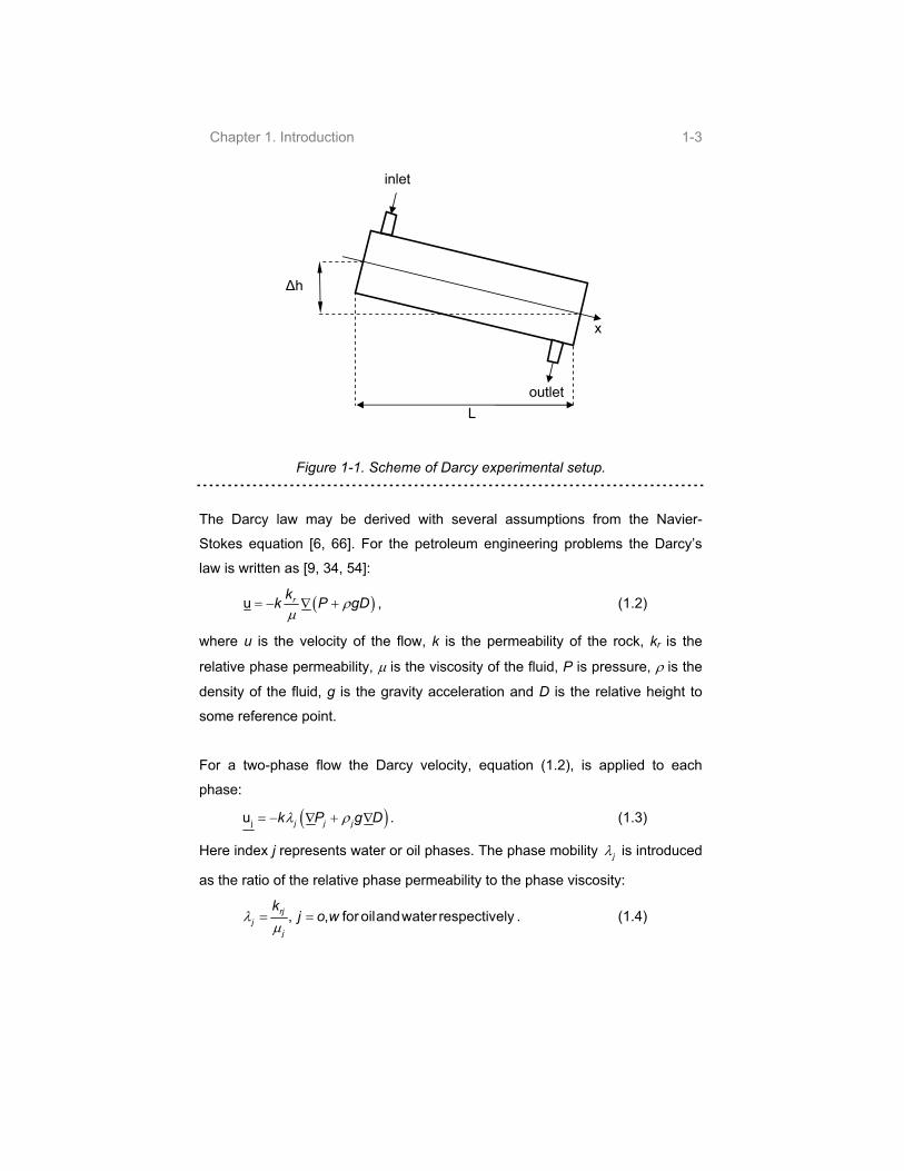
The history of the Darcy law starts at 1856, when Darcy [31] was working with
the flow characteristics of the sand filters. Darcy performed an experimental
study of the problem and founded the quantitative theory, which finally became
known as the Darcy law:
cA hQ
L. (1.1)
Here Q is the flow rate, A is the cross-sectional area of the media, is the
difference between fluid heads at the inlet and the outlet faces of the media in
the meters to water and L is the length of the media, see Figure 1-1. The
coefficient c characterises the velocity of the flow through the unit of area, under
the unit gradient of the flow head and is called the filtration coefficient.
h
Chapter 1. Introduction 1-3
inlet
outlet
x
L
h
Figure 1-1. Scheme of Darcy experimental setup.
The Darcy law may be derived with several assumptions from the Navier-
Stokes equation [6, 66]. For the petroleum engineering problems the Darcy’s
law is written as [9, 34, 54]:
u rkk P gD , (1.2)
where u is the velocity of the flow, k is the permeability of the rock, kr is the
relative phase permeability, is the viscosity of the fluid, P is pressure, is the
density of the fluid, g is the gravity acceleration and D is the relative height to
some reference point.
For a two-phase flow the Darcy velocity, equation (1.2), is applied to each
phase:
ju j j jk P g D . (1.3)
Here index j represents water or oil phases. The phase mobility j is introduced
as the ratio of the relative phase permeability to the phase viscosity:
, , for oilandwater respectivelyrj
j
j
kj o w . (1.4)

Chapter 1. Introduction 1-4
The total velocity is introduced as a sum of the velocities of water and oil
phases:
tu w w w o o ok P g D k P g D . (1.5)
Neglecting the capillary pressure, P=Pw=Po:
tu t gk P D
o
, (1.6)
here
t w (1.7)
is the total mobility, and
g w w o o g (1.8)
is the total gravity mobility.
For the incompressible fluids, flowing through the incompressible reservoir rock
the gradient of the total velocity at any point in the reservoir away from sinks or
sources must be equal to zero:
tu 0 . (1.9)
Introducing the total velocity, equation (1.6):
0t gk P D . (1.10)
However, in the vicinity of the wells, equation (1.10) should be written as:
t gk P D sq , (1.11)
here qs represents the well volumetric flow rate.
The mass conservation equation is represented by the so-called saturation
equation. Phase saturation is the fraction of the pore volume taken by the given
phase. For a two phase flow it is sufficient to resolve the mass conservation law
for any of the two phases, since:
1. (1.12) w os s
Here s is saturation, subscript o defines oil phase and subscript w defines water
phase.

Chapter 1. Introduction 1-5
For the immiscible incompressible black oil simulation the mass conservation
equation is typically solved for the water phase [9, 17, 68, 70]:
wuws
t0 . (1.13)
Here is porosity, sw is the water saturation, t is time, uw is the velocity of the
water phase.
All methods of reservoir simulation are based on solving a system of equations,
comprised of so-called pressure (1.11) and saturation (1.13) equations:
wu 0
t g
w
k P D
s
t
sq
(1.14)
The system of equations (1.14) may be solved in the discretised form on a
finite-difference (FD) grid, using various solution methods. One of the solution
methods is the Fully Implicit [17, 52] method. Using the fully implicit procedure
the governing system of equations (1.14) is simultaneously solved for all the
unknowns in all the gridblocks. It can be shown that this solution consists
entirely of pressures and functions evaluated at the new time step and therefore
is stable for any given time step size. However, the time step of the numerical
solver may be restricted in case of strongly non-linear fractional flow function
[52, 55]. The fully implicit formulations generally have a tendency toward high
numerical dispersion effects [25]. Another solution method is the IMPES
(Implicit Pressure Explicit Saturation) method [5, 26]. In this method the solution
procedure is divided into two steps. First the pressure is implicitly solved in
space and the flow velocity is found; afterwards the saturation values are
updated explicitly. During the implicit pressure solution the phase mobilities are
treated explicitly. As a result the time step size of the IMPES method is
restricted to handle the non-linearities of phase mobilities [5, 27, 28, 52, 76].
The time step size must be restricted so that the displacement front propagates
not more than one grid block per single time step. The IMPES solutions may
become extremely slow when applied to complex three-dimensional
Chapter 1. Introduction 1-6
displacement problems. However, the IMPES methods are less affected by the
numerical dispersion compared to the Fully Implicit methods. An Advanced
Implicit (AIM) method [36, 52, 61-63, 73, 74, 79] is introduced to combine the
strong points of both the fully implicit and the IMPES methods. The AIM method
uses an implicit solution procedure for the grid blocks in the “difficult” region,
typically, around the displacement front and an IMPES solution procedure for
the rest of the reservoir.
The streamline simulators are based on the IMPES solution procedure. The
outline of the IMPES solution procedure is presented below:
1. A reservoir is divided into a number of grid blocks in x, y and z directions.
Each grid block is assigned the porosity, the permeability and the initial
water saturation values;
2. The equation (1.11) is solved implicitly for the pressure values in all grid
blocks.
3. The water velocity is subsequently calculated in all grid blocks, using the
Darcy velocity equation (1.6);
4. The equation (1.13) is solved for the water saturation in all grid blocks;
5. The solution procedure returns to step 2 for the next time step.
1.2. Physics of capillary effects
For the flow of two or more immiscible fluids in porous media it is necessary to
consider the effect of the forces acting on the fluid contact interface.
A water molecule surrounded by other water molecules has a zero net attractive
force. On another hand, a water molecule on the interface of the fluid contact
has two different forces acting on it – one from the underlying water molecules,

Chapter 1. Introduction 1-7
another from the oil molecules lying directly above the interface. The resulting
force is unbalanced, creating the interfacial tension. For the problems of the
fluid flow in porous media it is important to consider not only the interface
between two fluids, but the interface between the fluids and a solid surface [4,
34]. The equilibrium of the forces acting on a bubble of a fluid on a surface
immersed into another fluid is presented below:
ws ns
wn
Figure 1-2. Drop of wetting fluid on the surface immersed into another fluid.
In Figure 1-2 is the interfacial tension; index s defines solid; index w defines
wetting phase; index n defines non-wetting phase; is the contact (wetting)
angle. By convention the contact angle is measured through the denser liquid
phase. The cosine of the contact angle may be found as [4, 34, 75]:
cos ws ns
wn
, (1.15)
The above equation is a rough approximation and does not take into account
many factors as, for example, roughness of the surface [1]. Moreover it may
give values of the cosine of the wetting angle higher than unity, which
corresponds to the formation of the wetting phase film on the surface.
The term wetting is used for the phase which tends to have a bigger contact
with the surface. Wettability is related to the system of two fluids and the
surface, see Figure 1-3.
water mercuryair
Figure 1-3. Drops of different fluids on the surface.
For example, in case of water / air system in contact with a wooden table the
water is the wetting phase. For the mercury / air system and the same table the
Chapter 1. Introduction 1-8
air is the wetting phase. This explains the difference in the outlook of the liquid
drops on the same surface.
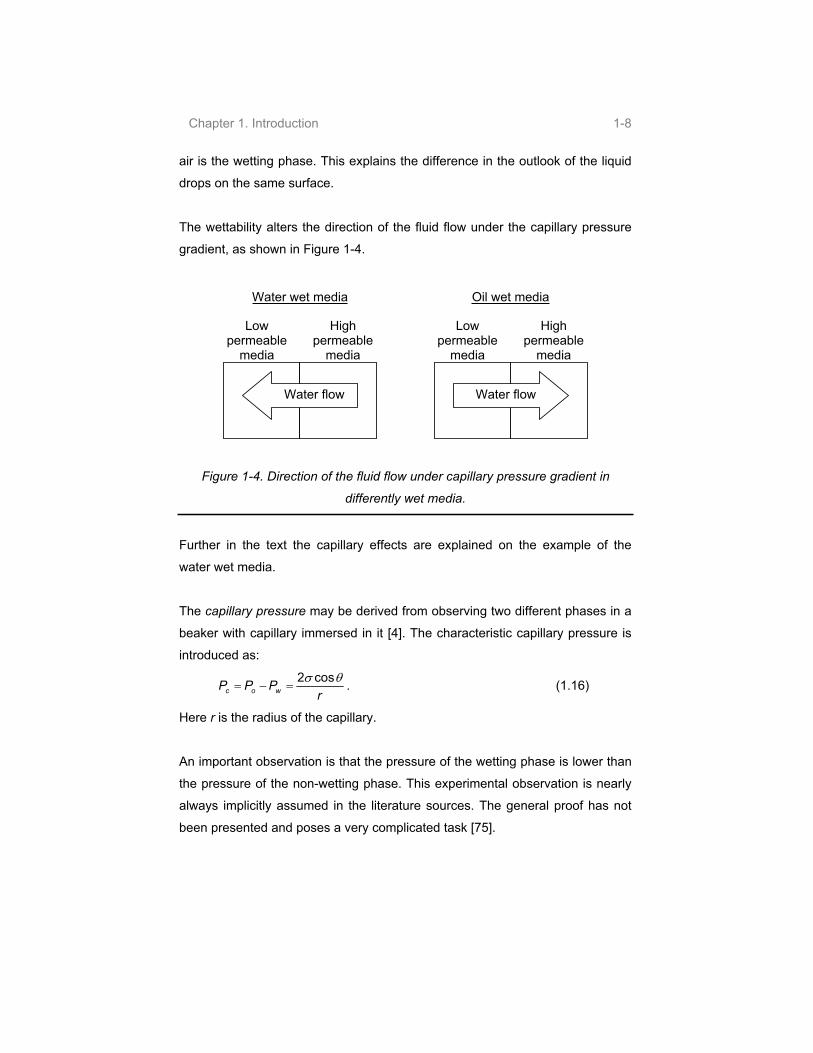
The wettability alters the direction of the fluid flow under the capillary pressure
gradient, as shown in Figure 1-4.
Lowpermeable
media
Highpermeable
media
Water flow
Water wet media
Lowpermeable
media
Highpermeable
media
Water flow
Oil wet media
Figure 1-4. Direction of the fluid flow under capillary pressure gradient in
differently wet media.
Further in the text the capillary effects are explained on the example of the
water wet media.
The capillary pressure may be derived from observing two different phases in a
beaker with capillary immersed in it [4]. The characteristic capillary pressure is
introduced as:
2 cosc o wP P P
r. (1.16)
Here r is the radius of the capillary.
An important observation is that the pressure of the wetting phase is lower than
the pressure of the non-wetting phase. This experimental observation is nearly
always implicitly assumed in the literature sources. The general proof has not
been presented and poses a very complicated task [75].

Chapter 1. Introduction 1-9
Furthermore, the model of parallel capillary bundles [34] is often used to
represent the structure of the porous media. This model is based on the
simplification of porous media to the set of the tortuous cylindrical capillary with
the constant radii of each capillary. Permeability of the ideal cylinder is
evaluated as:
4
8
rk n , (1.17)
porosity as:
2n r . (1.18)
Here n is the concentration of the capillaries per unit of the area.
Dividing equation (1.17) by equation (1.18) the radius of a pore can be obtained
in terms of porosity and permeability:
2 2k
r (1.19)
Equation (1.19) is derived using the Carman-Kozeny model. In reality the
shapes of the capillaries diverse from the ideal cylinders. Using equations (1.16)
and (1.19) a characteristic value of the capillary pressure, within an order of
magnitude, may be obtained:
coscP
k. (1.20)
Leverett [47] proposed a modification to the capillary pressure equation to
convert all capillary-pressure data to a single universal curve. So-called Leverett
or J-function is introduced as a function of the saturation of any of the two
phases. Capillary pressure equation is obtained as:
coscP J
kws . (1.21)
In fact there is a significant difference in the correlation of the J-function to the
saturation from formation to formation, so that no universal curve is found.
Figure 1-5 sketches the displacement processes typical for an oil reservoir.
Initially the reservoir is fully saturated with water. During oil migration water is
displaced by oil in the process called the primary drainage. During the oil
recovery oil is displaced by the injected water in the process called the

Chapter 1. Introduction 1-10
imbibition. If water is to be displaced by oil again, for example in the laboratory
experiments, the displacement process is called the secondary drainage.
0 swi 1-sor 1 swater
J-f
unction
Figure 1-5. Typical shapes of the J-function for primary drainage (dashed line),
imbibition (solid line) and secondary drainage (dotted line).
During the imbibition or the secondary drainage the saturation of the displaced
fluid decreases to a non-zero value. At this non-zero saturation the displaced
fluid becomes immobile. The minimum mobile oil concentration is called
irreducible oil saturation. The minimum mobile water saturation is called initial
water saturation. The term initial water saturation is used in relation to the
imbibition process. Non-zero initial water and irreducible oil saturations are due
to the fact that each phase can be mobile only while it is continuous. Parts of
water or oil may be trapped inside another phase and therefore become
immobile [11, 34]. The mechanisms of formation of the trapped oil or water
ganglia are presented and discussed in [11, 19].
The main capillary pressure effect is the redistribution of the phases inside
heterogeneous porous media. The wetting phase prefers to travel through the
low permeable porous medium since it provides larger contact area with the
surface [34]. Neglecting capillary effects may result in incorrect prediction of the
displacement profiles.
Chapter 1. Introduction 1-11
The capillary pressure also leads to the end-effects between the zones with
different permeability and in the vicinity of a production well. Due to the end-
effects the wetting phase is accumulated on the border in the low permeable
zone before breaking through into the high permeable medium [9, 34, 54]. The
increase of the water saturation in the low permeable boundary layer leads to
decrease of the capillary pressure (see Figure1-2) and therefore allows water to
penetrate into the high permeable zone. This effect may be observed in the
vicinity of a producer, where the capillary effects lead to the well-known fact of
drowning the well. The well, being a tube of several inches in diameter can be
considered as extremely high permeable medium, see the equation (1.17).
Therefore, as soon as water in the reservoir breaks through to the production
well, it is accumulated around the well due to the end-effects before penetrating
into the well. Laboratory tests [49] have also shown that water may flow in the
low permeable (water-wet sample) medium without penetrating into the high
permeable one until the low permeable medium is completely swept.
The importance of the capillary forces may be estimated by means of several
groups of dimensionless parameters [9, 80]. These dimensionless groups allow
estimating a relation of the average viscous to the average capillary forces.
However, even when the dimensionless parameters show that the displacement
is viscous dominated, the capillary forces may be locally dominating, for
example in the vicinity of the displacement front or on the borders of the zones
with different permeability.
Capillary effects are rather complicated. One of the difficulties both for the finite-
difference and the streamline methods is the capillary limitation of the stable
time step size.
The capillary pressure poses an additional problem for the streamline methods.
Capillary as well as gravitational forces often act across the streamlines
therefore the operator splitting solution is required. The operator splitting
solution is described in detail in Section 2.2. Moreover, unlike gravity no uniform
direction of the capillary forces can be found. Tracing the "capillary lines" seems

Chapter 1. Introduction 1-12
to be a very complicated task therefore the operator splitting step is performed
on the finite difference grid.
1.3. Introduction to Streamline Simulation
The introduction starts with an outline of the 3DSL 0.25 streamline simulator (by
R.P. Batycky, SUPRI-C, Department of Petroleum Engineering, Stanford).
Later an overview of the streamline methods development history is presented.
The overview is divided into three parts: Introduction of streamlines and early
stage of the development; Development of the streamline methods; Modern
advances in the streamline methods.
The overview mentions only the most relevant works for the current project.
Many other researchers and scientists contributed to the development of the
streamline methods.
1.3.1 Outline of the 3DSL 0.25
Figure 1-6 outlines the structure of the 3DSL 0.25 streamline simulator. More
information on the individual steps of the 3DSL 0.25 scheme may be found
further in the text.
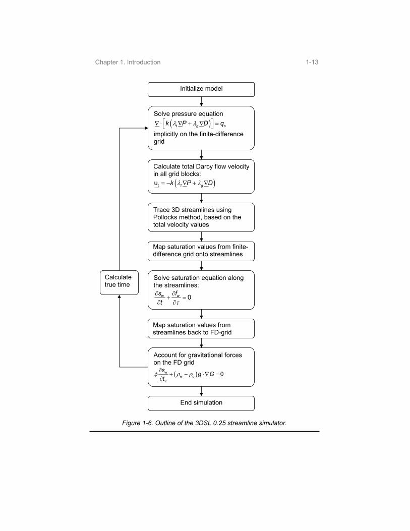
Chapter 1. Introduction 1-13
Initialize model
Solve pressure equation
t g sk P D q
implicitly on the finite-difference grid
Calculate total Darcy flow velocity in all grid blocks:
tu t gk P D
Trace 3D streamlines using Pollocks method, based on the total velocity values
Map saturation values from finite-difference grid onto streamlines
Solve saturation equation along the streamlines:
0w ws f
t
Map saturation values from streamlines back to FD-grid
End simulation
Calculatetrue time
Account for gravitational forces on the FD grid
2
0ww o
sg G
t
Figure 1-6. Outline of the 3DSL 0.25 streamline simulator.

Chapter 1. Introduction 1-14
1.3.2. Introduction of streamlines and early stage of development
The term streamfunction was first used by Muskat in 1937 [54] in petroleum
engineering studies for analysis of the two-dimensional steady state flows from
the finite line sources into an infinite sand. Muskat used the analytical function
of the complex variable z=x+iy to introduce the Darcy velocity and the
streamfunction potentials. Streamlines were introduced as lines of constant
streamfunction, tangent to the fluid velocity vector in any given point. In the
static case a streamline illustrates one of the paths, which the particles of the
flow may take inside the porous media.
The next key moment in the streamline methodology is represented by three
papers by Higgins and Leighton in the early sixties [37-39]. Higgins and
Leighton simulated a quarter of a five-spot pattern in a homogenous reservoir,
containing one injector and one producer, as sketched in Figure 1-7.
inj
p p
pp
12
34
56
78
inj
p
Figure 1-7. Five-spot pattern. A quarter of a five-spot pattern with streamlines.
The simulation space was divided into the flow channels, or streamtubes
(indicated with numbers 1 to 8 in Figure 1-7), bounded by nine analytically
calculated streamlines (dashed lines in Figure 1-7). The streamtubes remained
constant throughout the whole simulation time. To account for the changes of
the fluid mobilities, Higgins and Leighton introduced the flow resistance
parameter for every channel [37]. The authors presented a method to forecast
three-phase flow [38] in complex geometry. The method was implemented to
simulate the specific five-spot waterflood of a partially depleted stratified oil

Chapter 1. Introduction 1-15
reservoir. The reservoir was divided into set of layers without any cross-flow
between them. Field performance was determined as a sum of performances of
individual layers. The papers also described Higgins – Leighton method, which
did not require calculations of the individual pressures, as the resistance to flow
in each channel in the flow pattern was readily determined without using the
iterations.
Martin and Wegner [50] reported that the method suggested by Higgins and
Leighton failed for water-to-oil mobility ratios smaller than one ( 1w o ). The
source of an error was found to be the assumption of the streamlines being
independent upon the mobility ratio. Martin et al. suggested to periodically
update the streamtubes. Periodic updates of the streamtubes created non-
uniform initial conditions and required numerical solution along them. The
suggested method dramatically increased the quality of the predictions for the
simulations with mobility ratios less than one. The streamlines were updated
using numerical or analytical methods involving the pressure and the
streamfunction solution.
1.3.3. Development of the streamline method
Pollock [57] presented a semi-analytical flow path tracing method for finite-
difference models. This semi-analytical method allowed tracing the streamlines
in complex displacement cases. To trace the streamlines from the block inlet
face to the block outlet face (see Figure 1-8) the following routine was
suggested:
Evaluate average velocity on a grid block face by dividing the volumetric
flow rate through the face by the cross-sectional area of the face and the
porosity in the cell;
Compute the velocity at any point in the grid block by means of the linear
interpolation of the grid block face velocities;
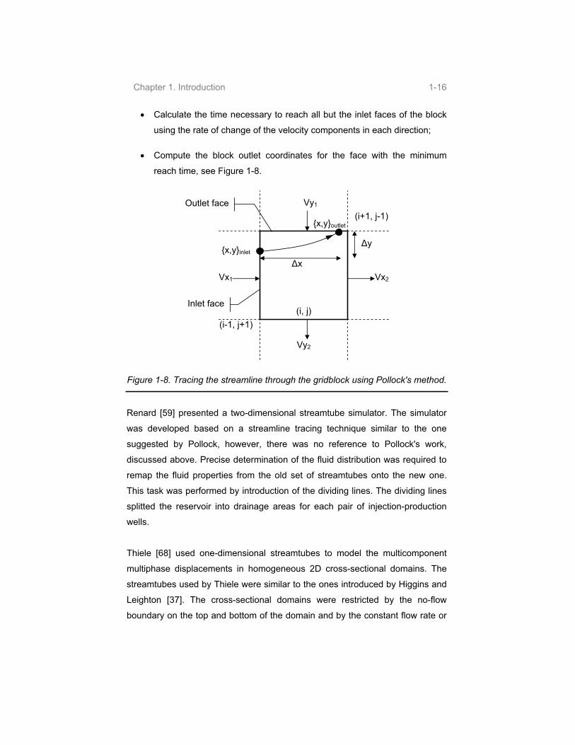
Chapter 1. Introduction 1-16
Calculate the time necessary to reach all but the inlet faces of the block
using the rate of change of the velocity components in each direction;
Compute the block outlet coordinates for the face with the minimum
reach time, see Figure 1-8.
Vx1
(i, j)
(i-1, j+1)
Vy2
(i+1, j-1)
Vx2
Vy1
{x,y}inlet
{x,y}outlet
x
y
Inlet face
Outlet face
Figure 1-8. Tracing the streamline through the gridblock using Pollock's method.
Renard [59] presented a two-dimensional streamtube simulator. The simulator
was developed based on a streamline tracing technique similar to the one
suggested by Pollock, however, there was no reference to Pollock's work,
discussed above. Precise determination of the fluid distribution was required to
remap the fluid properties from the old set of streamtubes onto the new one.
This task was performed by introduction of the dividing lines. The dividing lines
splitted the reservoir into drainage areas for each pair of injection-production
wells.
Thiele [68] used one-dimensional streamtubes to model the multicomponent
multiphase displacements in homogeneous 2D cross-sectional domains. The
streamtubes used by Thiele were similar to the ones introduced by Higgins and
Leighton [37]. The cross-sectional domains were restricted by the no-flow
boundary on the top and bottom of the domain and by the constant flow rate or

Chapter 1. Introduction 1-17
pressure on either end of a domain. Non-linearity of the underlying flow field
was taken into account by periodically updating the streamtubes. The
streamtubes were updated based on the values of the streamfunction. Thiele
reported that unlike the streamlines, the streamtubes offered the visual
interpretation of the local flow velocity - thick sections of a streamtube
corresponded to the slow flow regions, thin sections to the fast flow regions.
The streamfunction for a three-dimensional case was presented by Matanga
[51]. The streamtubes in three-dimensions were formed by the streamsurfaces,
not the streamlines as in two-dimensional case. The interception of two
streamsurfaces gave a streamline. However, the 3D streamfunction was shown
to be rather complicated.
Tracing streamlines in three dimensions does not pose any additional
complications comparing to a two-dimensional case. A possibility to combine
the strong points of both methods: ease of streamline tracing and flow velocity
information from streamtubes was presented in the work by Datta-Gupta and
King [32]. The “time-of-flight” concept was introduced along the streamlines.
This concept allowed representing the flow velocity without using the
streamtubes. The time of flight represented the travel time of a particle to the
certain point along the streamline, see Figure 1-9.
injector
producer
2
1
t2 > t1t1 time of flight to point 1 t2 time of flight to point 2
Figure 1-9. Time of flight from the injector along the streamline to the producer.

Chapter 1. Introduction 1-18
The time-of-flight in the differential form was introduced as [18, 32]:
tus. (1.22)
Moreover time of flight allowed to transform the three-dimensional saturation
equation (1.13), to the one-dimensional equation in the time of flight coordinates
along the streamlines:
0w ws f
t, (1.23)
where
ww
w o
f . (1.24)
It is important to point out, that the streamlines were traced taking into account
the effects of porosity, permeability and the pressure gradient. The time of flight
variable accounted for the total velocity and the reservoir porosity. This allowed
one dimensional equation (1.23) to be independent upon any reservoir
properties.
The streamline method was extended to true 3D systems, including longitudinal
and transverse diffusion and gravitational effects in FCM displacements by
Blunt et al. [18]. The gravitational effects were included in the step of tracing the
streamlines by solving the pressure equation with gravitational effects. The
saturation equation accounted for the gravitational effects as well:
tuww w o
sf g
t0G . (1.25)
Here w o
w o
G , (1.26)
and g g D . (1.27)
The equation was transformed to the form of:
vww
sf
t0 . (1.28)
Here tv u w o
w
Gg
f (1.29)
The time-of-flight was introduced in terms of v rather than ut:

Chapter 1. Introduction 1-19
vs. (1.30)
As a result the equation (1.23) was obtained, minimizing the necessary
modifications of the streamline simulator to account for the gravitational forces.
Thiele et al. [69] presented a three-dimensional two-phase streamline results
and extended the method to multi-well simulations with changing mobility fields.
Reported modifications were essentially a continuation of the Thiele's PhD work
[68]. The 3D displacements were modeled using the streamlines with time of
flight concept, rather than the streamtubes.
The simulator was further extended to the compositional version neglecting the
gravitational effects [70]. The compressibility of the fluids was accounted only
along the streamlines. The pressure was considered incompressible.
Gravity very often acts across the main direction of the flow and, therefore,
across the streamlines. Accounting for the gravitational effects only along the
streamlines may lead to underestimation of the gravity cross flow. To account
for the gravity cross flow, Bratvedt et al. suggested using an operator splitting
method [21]. The equation (1.25) was solved in two consecutive steps. First the
saturation was solved along the streamlines with respect to the viscous forces
only, equation (1.23). The gravitational effect was accounted for in the second
step on the finite difference grid:
2
0ww o
sg G
t, (1.31)
Here index 2 indicates the second step of the operator splitting method.
Another significant difference of the streamline simulator developed by Bratvedt
was utilization of the front-tracking method for resolving the saturation equation
(1.23). The key principle of the front-tracking method is to represent the
saturation front as a step function with a set of discontinuous fronts. The step
function converges towards the physical continuous solution with increase of
number of fronts. The reported advantages of the front tracking methods were:
1) less smearing of the front; and 2) independence of the numerical solution of a

Chapter 1. Introduction 1-20
grid, leading to a method not limited by the CFL (Courant-Freidrichs-Levi [76])
stability condition [20, 21].
Batycky’s PhD thesis [8] resulted in the three-dimensional two-phase field-scale
streamline simulator (3DSL 0.25). The gravitational effects were accounted for
using the operator splitting method. The gravity step was performed by tracing
the so-called gravity lines for each vertical column of the grid blocks. Batycky
has assigned the volumetric flow rate to each streamline. This allowed treating
each streamline as a centerline of an imaginary streamtube. The volume of
such a streamtube was found by multiplying the volumetric flow rate along the
streamline by the time of flight.
The 3DSL 0.25 also utilized the "True time" concept. This concept required
calculating the "true" time step size using the cumulative water balance during
the current time step:
1
, , , ,
1 1
1 1 2 1
n nn
water initial water in place water injected water produced
i itrue n n
w
V V V V
tQ f
.
(1.32)
Here t is time, V is volume, Q is flow rate, superscript n denotes time step, and
1 2 1 2n n nf f f is the average field production fractional flow function.
1.3.4. Recent advances in streamline simulation
The latest advances in streamline simulation were performed in the several
directions.
Bedrikovetsky et al. [9] suggested an analytical three-dimensional two-phase
streamline simulator using curvilinear coordinates. The paper presented the
transformation from the Cartesian to the curvilinear coordinates, resulting in the
dispersion free, fast analytical solution neglecting capillary and gravitational
effects.

Chapter 1. Introduction 1-21
Di Donato et al. [33] recently presented a dual-porosity streamline simulator,
based on the 3DSL two-phase black-oil version. The dual-porosity simulation
system was composed of a flowing fraction, representing the fracture network
and the matrix, representing the relatively stagnant regions. In this model the
streamlines capture the movement through the fracture system while the
transfer of fluids from the fracture into the matrix was accounted for using a
transfer function:
;
.
wf wf
f
wm
m
s f T
t
s T
t
(1.33)
Here index f denotes the properties of the fracture region and index m of the
matrix, T stands for the transfer function.
The authors concluded that when the appropriate transfer function and the
shape factors are applied, the simulation results were in a good agreement with
the commercial finite-difference simulator Eclipse [62, 63]. For the million grid
block models the dual porosity streamline simulator was orders of magnitude
faster, compared to the finite difference simulators.
Al-Hutheli and Datta-Gupta [3] presented a dual-porosity dual-permeability
streamline simulator, accounting for the flow both through the fractures and
through the matrix. The transfer between the fracture and the matrix was
accounted for using the transfer function. The transfer function was resolved by
the operator splitting method on the finite-difference grid. The authors reported
a close match with Eclipse simulator and significant speed-ups comparing to
Eclipse especially for the simulation on the large grids.
Crane et al. [30, 64] presented a fully compositional streamline simulator
accounting for gravitational effects by usage of the gravity lines, but neglecting
capillary effects. The method combined the streamline tracing method with 1D
finite difference solver from Eclipse 300 [63] used along the streamlines and the
gravity lines. This method required two pressure field evaluations. The first time

Chapter 1. Introduction 1-22
the pressure field was evaluated on the finite difference grid. The pressure
values obtained were used to trace the streamlines. The second time the
pressure field was evaluated during the 1D finite-difference solution along the
streamlines. The pressure solution, received along the streamlines, was
mapped back to the finite difference grid along with the saturation solution. The
authors reported a significant speed advantage over Eclipse on the large grids.
However introduction of the gravitational effects resulted in the slow down of the
streamline simulator and some additional stability problems compared to the
streamline method neglecting the gravitational effects.
A lot of effort has been done in the area of the compositional streamline
simulation. Seto et al. [65] presented a field scale compositional streamline
simulator and Jessen and Orr [43] presented the detailed analysis of the gas
cycling and the development of the miscibility in condensate reservoirs. Jessen
and Orr concluded that using the one-dimensional analytical solver along the
streamlines resulted in fast, dispersion free solutions, comparable to the finite-
difference simulations on much finer grids. For the 3D simulations [65] the
streamline simulator was two or three orders of magnitude faster than Eclipse
300. The outcome of the dispersion free analytical solution was a lower
recovery prediction, because the dispersion associated with finite-difference
solutions resulted in optimistic sweep efficiency. Seto et al. [65] also concluded
that the introduction of the gravitational and capillary effects as well as
streamline updating for the 3D compositional cases are important research
areas. The description of the 3D compositional streamline reservoir simulator
was given by Jessen and Orr [42]. A detailed description of the analytical 1D
multicomponent solution along the streamlines may be found in Jessen et
al. [41].
Jessen and Orr [44] have further developed compositional streamline simulation
to include the gravitational effects. The method of accounting for the gravity
segregation using the pseudo-immiscible gravity step marginally added to the
overall CPU requirement. The pseudo-immiscible approach requires a phase
flash only before the gravity step. After the phase flash each individual phase
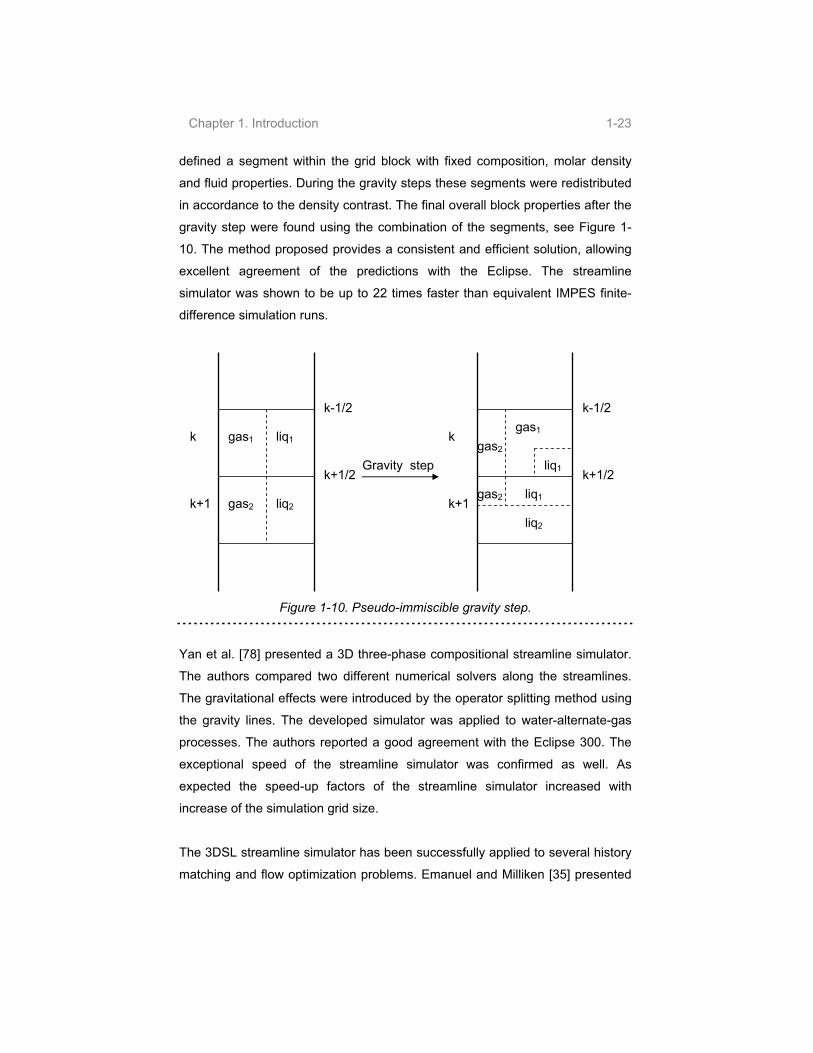
Chapter 1. Introduction 1-23
defined a segment within the grid block with fixed composition, molar density
and fluid properties. During the gravity steps these segments were redistributed
in accordance to the density contrast. The final overall block properties after the
gravity step were found using the combination of the segments, see Figure 1-
10. The method proposed provides a consistent and efficient solution, allowing
excellent agreement of the predictions with the Eclipse. The streamline
simulator was shown to be up to 22 times faster than equivalent IMPES finite-
difference simulation runs.
gas1
gas2
liq1
liq2
k
k+1
k-1/2
k+1/2Gravity step
gas1
gas2
liq1
liq2
k
k+1
k-1/2
k+1/2
gas2
liq1
Figure 1-10. Pseudo-immiscible gravity step.
Yan et al. [78] presented a 3D three-phase compositional streamline simulator.
The authors compared two different numerical solvers along the streamlines.
The gravitational effects were introduced by the operator splitting method using
the gravity lines. The developed simulator was applied to water-alternate-gas
processes. The authors reported a good agreement with the Eclipse 300. The
exceptional speed of the streamline simulator was confirmed as well. As
expected the speed-up factors of the streamline simulator increased with
increase of the simulation grid size.
The 3DSL streamline simulator has been successfully applied to several history
matching and flow optimization problems. Emanuel and Milliken [35] presented
Chapter 1. Introduction 1-24
a method to match the individual well performance with assistance of the
streamline method. The streamlines helped to visualize the blocks, which were
affecting the well performance. This new method was named AHM (Assisted
History Matching). The same method was further applied to 105 – 106 grid block
simulations [53]. Authors concluded a successive history match with very
modest changes of the parameters in the model. The changes in the model
data were generally within uncertainty of the initial data.
Agarwal and Blunt [2] presented history matching results based on the 3DSL
code. The 3DSL was modified to handle the three phases flow as well as
compressibility and gravitational effects. Four modification were made: 1)
compressibility was introduced into the pressure equation; 2) the possibility of
tracing the streamlines which do not start in the injector and / or do not end up
in the producer due to the compressibility effects was introduced; 3)
compositions were mapped from the grid to streamlines and back, rather than
saturations; 4) a mass conservation equation was solved along each streamline
accounting for changes in pressure and the total velocity, similar to Craine et
al.[30] and Thiele et al. [70]. The history matching was based on changing the
permeability field. The relation of the permeability change to the change in time
of flight was used to compute the next permeability field. A reasonable history
match and predictions has been achieved.
The recent publication by Thiele and Batycky [72] showed an application of the
3DSL to the water injection optimization. The reported advantages of the
streamline method for this task were the simulation speed and the fact that the
streamlines readily provided a snapshot of how the reservoir was connected.
The efficiency of each injector was determined as a ratio of the water injected
into it to the oil produced from the offset wells. The water was than redistributed
from the low efficiency wells into the high efficiency wells, allowing the higher
total field oil production for the same total amount of water injected.
Several attempts to introduce the capillary forces have been performed as well.
Berre et al. [16] presented a two-dimensional two- and three-phase front-
Chapter 1. Introduction 1-25
tracking streamline simulator with capillary effects. However, the capillary
effects are accounted by specifying the simplified capillary pressure / diffusion
term rather than capillary pressures between phases.
Rodriguez et al. [60] presented a three-dimensional streamline simulator with
capillary effects, neglecting the gravity. The simulator was based on the
streamline ideas presented by Batycky in his PhD thesis [8]. The developed
simulator was applied only to a simple synthetic simulation case.
The capillary effects did not received proper attention in the streamline
development. Therefore it is very important to provide a way to account for
capillary effects in streamline simulation.
Detailed overviews of the streamline simulation are also given by King and
Datta-Gupta [46], Batycky [8] and Thiele [71].

2-1
Chapter 2. Mathematical models
This chapter presents the modifications to the governing IMPES equations to
account for capillary effects. The modifications of the governing pressure
equation are presented first, followed by the saturation equation modification.
The modified streamline simulation scheme is presented. The numerical
solution of the modified systems of equations is given. The possibilities for the
material balance errors are discussed. Automatic time step selection algorithms
are presented.
The chapter concludes with a simple simulation case illustrating the effects of
the modification of the governing system of equation.
2.1. Modification of the governing system of equations
The governing system of equations is introduced in the Section 1.1, equation
(1.14). The necessary modifications to the governing system of equations to
account for capillary effects are presented below.
2.1.1. Pressure equation with capillary effects
The pressure equation is a momentum conservation law. Derivation of the
pressure equation with respect to capillary effects is presented below. As it is
stated in Section 1.1, the divergence of the total velocity for the incompressible
case must remain zero at any point in a reservoir far from the wells, equation
(1.9). The total velocity with respect to capillary pressure is described by the
equation (1.5). Using the capillary pressure equation (1.21), the oil pressure is

Chapter 2. Mathematical model 2-2
substituted by the capillary pressure and the water pressure. Regrouping the
phase mobilities:
tu t w o c gk P P D . (2.1)
The divergence of the total velocity is than obtained as:
0t w o c gk P P D . (2.2)
Here k is permeability; represent the mobilities, as introduced in Chapter 1; Pc
is the capillary pressure, D is the depth.
2.1.2. Capillary-viscous potential
It is possible to reformulate the pressure equation (2.2) to improve the stability
of the numerical solution method and the handling of the sharp variation of the
reservoir properties.
Basing on the capillary pressure equation (1.21), the new variable is introduced:
cos
k. (2.3)
This new variable is dependent only upon the properties of the porous media
and independent of the saturation. Therefore the capillary pressure may be
represented by the product of and the saturation dependent Leverett function
J(s). The gradient of the capillary pressure is then obtained as:
cP J s J s . (2.4)
The gradient depends only upon the reservoir properties. The gradient is
responsible for the transfer of the fluids between the zones with different
permeability and / or wettability. The gradient of the Leverett function J acts
mostly in vicinity of the saturation fronts.
Introduction of the equation (2.4) into the pressure equation (2.2) gives:
0t w o o gk P J s J s D . (2.5)
It is convenient to reformulate the multipliers in front of the J and in terms
of total mobility:

Chapter 2. Mathematical model 2-3
1 1t w wo t w t t t w
t t
f . (2.6)
Here fw is the water fractional flow function, equation (1.24).
Substituting the oil phase mobility from equation (2.6) into equation (2.5):
1
1 0
t w w
t w g
k P f J s
k f J s D . (2.7)
The capillary-viscous potential (CVP) [15] is introduced as:
0wP J s s , (2.8)
where
0
wi
s
s
s f dJ s . (2.9)
The gradient of the is obtained as: 0
0
wi
s
s
s f dJ s f J s . (2.10)
Gradient of the potential may be found as:
0 1wP J s s f J sw. (2.11)
Introducing the CVP gradient, equation (2.11) into the pressure equation (2.7)
and collecting terms it may be obtained, that:
0 0t t gk k s fJ s k D . (2.12)
For convenience,
0s s fJ s (2.13)
and, therefore:
0t t gk k s k D . (2.14)
Solution of equation (2.14) is very similar to the solution of the straightforward
pressure equation (2.2) (SFD method) and requires modest changes to the
streamline code.
The total velocity in terms of the CVP is formulated as:
tu t t gk s D . (2.15)

Chapter 2. Mathematical model 2-4
Introduction of the potential makes it possible to reformulate the pressure
equation in such a way that the spatial variation of saturation is taken into
account inside the capillary-viscous flow potential. This facilitates easier
handling of zones with strong saturation and / or permeability variation.
If the porous medium were homogeneous, the proposed modification leads to
the pressure equation, which is identical to the equation without capillary forces.
2.1.3. Saturation equation with capillary and gravity effects
The mass balance equation is represented by the saturation equation. The
saturation equation is derived from equation (1.13) with respect to capillary
pressure [9]. The water pressure gradient may be expressed from equation
(2.1) in terms of capillary pressure and the total velocity:
t
1u 1
g
w w c
t t
P f Pk
D . (2.16)
Introducing the pressure gradient into the Darcy velocity for the water phase,
equation (1.2)
w t
1u u 1
g
w w c w
t t
k f P Dk
g D . (2.17)
Regrouping the variables:
w tu u 1gw
w w c w w w
t t
k f P k g D . (2.18)
Considering equation (1.24) and using equation (1.7):
1 1 w oww w
t t
f . (2.19)
The gravity term may be simplified as well using equation (1.7) and (1.8):
g w w w o o w o w w
w w w
t t
g gg
t
. (2.20)
Regrouping the terms in equation (2.20):
g o ww w w o w
t t
g g . (2.21)

Chapter 2. Mathematical model 2-5
Introducing equations (2.19) and (2.21) into (2.18):
w tu u w o o ww c o w
t t
f k P k g D . (2.22)
Introducing the water velocity from the equation (2.22) into the saturation
equation (1.13):
tu 0w o o www c o w
t t
sf k P k g D
t. (2.23)
Regrouping and using the incompressibility assumption, equation (1.9):
tu 0w o o www c o w
t t
sf k P k g D
t.
(2.24)
The equation (2.24) simplifies to the Rapoport – Leas equation [58] if the gravity
is neglected. Neglecting the capillary effects as well results in the Buckley –
Leverett equation [22].
2.1.4. Final systems of equations
The SFD method and the CVP formulation result in different governing system
of equations. For the SFD method the governing system of equations is
comprised of the pressure equation with capillary effects (2.2) and the
saturation equation with capillary effects (2.24).
t
0
u 0
t w o c g
w o o www c o w
t t
k P P D
sf k P k g D
t
(2.25)
The governing system of equations for the CVP formulation is constructed from
the CVP equation (2.14) and the saturation equation with capillary effects
(2.24).
t
0
u 0
t t g
w o o www c o w
t t
k k s k D
sf k P k g D
t
(2.26)

Chapter 2. Mathematical model 2-6
Further in this chapter the discretization and the solution methods of the
governing equations are discussed.
2.2 Solution of the governing systems of equations with
capillary and gravity forces
The outline of the streamline simulator with capillary effects (CapSL) is
presented below. Further in the text the details of the numerical solution are
discussed.
2.2.1. Outline of the modified streamline simulator
The following scheme outlines the structure of the CapSL 2.0 streamline
simulator. The blocks which are unchanged, compared to the 3DSL 0.25
scheme (Figure 1-3) have dark gray background; the modified blocks have light
gray background; the new blocks have white background.
The discussion of the various numerical solution methods follows the solution
scheme in Figure 2-1. The numerical representation of the pressure equation is
discussed first then followed by the saturation equation. The time step selection
and the mass balance error evaluation are discussed later on in this chapter.

Chapter 2. Mathematical model 2-7
Initialize model
Solve SFD pressure equation (2.2) or CVP equation (2.14)
Calculate total Darcy flow velocity in all grid blocks, equations (2.1) and (2.15), respectively
Trace 3D streamlines
Map saturation values from finite-difference grid onto streamlines
Solve saturation equation along the streamlines:
0w ws f
t
Map saturation values from streamlines back to FD grid
End simulation
Account for capillary and gravity forces on FD grid, equation (2.24)
Calculate massbalance error, eq. (2.68)
Next saturationstep
Next pressure
step?
no
yes
Reject thetime step anddecreasetime step size if necessary
Saturation step
Time step
Figure 2-1. Outline of the CapSL streamline simulator.

Chapter 2. Mathematical model 2-8
2.2.2 Numerical representation of the pressure equation
The pressure equation is solved implicitly using 7-point stencil (three
dimensions) on the Cartesian grid. The pressure is treated implicitly; the phase
mobilities, gravity and capillary forces are treated explicitly. Complete
description of the pressure equation discretization may be found in Aziz and
Settari [5], Mattax [52] and Batycky [8]. Here only the discretization of the
capillary pressure gradient is presented:
c co c o o o
P Pk P k k k cP
x x y y z z.
(2.27)
Explicit treatment of the capillary term means that the capillary pressure is
computed based on the saturation values from the previous time step [54]. The
finite difference approximation is written as:
, , , ,
x y z
c x x c y y c z z ci j k i j kC P C P C P C P .
(2.28)
Here is the capillary transmissibility, as shown below; index i corresponds to
the discretization along the x-axis, j along the y axis and k along the z axis.
Each term on the right hand side of equation (2.28) is expended using centered
second-difference equation [5, 56] for all grid blocks i,j,k:
1 2, , , 1 , 1 2, , , 1 ,
2
X X
i j k c i c i i j k c i c ijk jx
x x c
C P P C P PC P
x
k;
(2.29)
, 1 2, , 1 , , 1 2, , 1 ,
2
Y Y
i j k c j c j i j k c j c jy ik iky y c
C P P C P PC P
y;
(2.30)
, , 1 2 , 1 , , , 1 2 , 1 ,
2
Z Z
i j k c k c k i j k c k c kij ijz
z z c
C P P C P PC P
z.
(2.31)

Chapter 2. Mathematical model 2-9
The coefficients Cx, Cy and Cz are representing the inter-block transmissibility
for a block-centered grid. As it is stated by Aziz and Settari [5] there is no
unique way for obtaining the inter-block transmissibility term. Typically, the
harmonic averaging resulting in the most accurate prediction of the flow rate is
used. The harmonic averaging is derived from the assumption of the piecewise
constant interface transmissibility [5].
The transmissibility is introduced on an example of , , 1 2
z
i j kC as:
, , 1 2 1 2 , 1 2
1 2
z
i j k k o k
k
AC k
z. (2.32)
Here1 2kz is the distance between centers of two neighboring blocks, A is the
interface area between two blocks, and1 2 1 2k kk is the harmonic average of the
properties between the neighboring blocks, introduced as:
11 2 1 2
1
, 1 ,
k kk k
k k
k o k k o k
k
k k1
, (2.33)
here is the distance from the center to the interface. Equations (2.32) and
(2.33) may be used for the calculation of the transmissibilities at any interface,
not necessarily coinciding with block faces. For the inter-block interface:
2k
k
z. (2.34)
Introducing equation (2.34) into (2.33):
11 2 1 2
1
, 1 ,
k kk k
k k
k o k k o k
z zk
z z
k k1
. (2.35)
Introducing the harmonic average, equation (2.35) into the capillary
transmissibility, equation (2.32):
1, , 1 2
11 2
, 1 ,
k ki j k
k kk
k o k k o k
z zAC
z zz
k k1
. (2.36)
Considering that
11 2
2 2k k
k
z zz , (2.37)
the capillary transmissibility is obtained as:
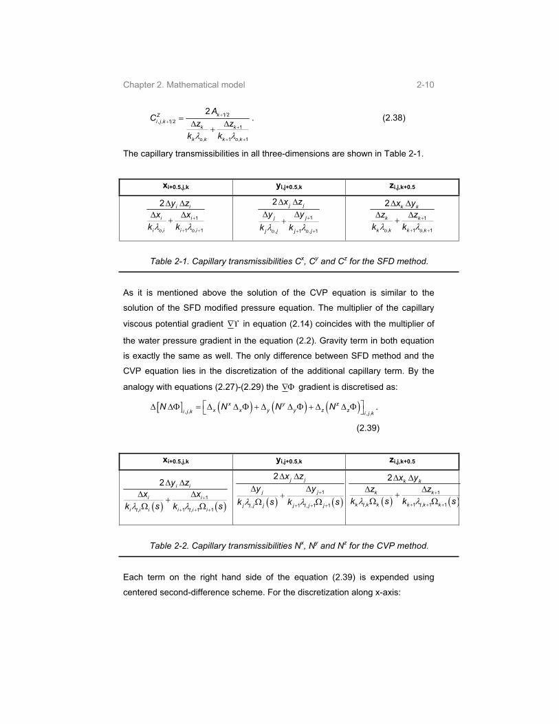
Chapter 2. Mathematical model 2-10
1 2
, , 1 21
, 1 ,
2kZ
i j kk k
k o k k o k
AC
z z
k k 1
. (2.38)
The capillary transmissibilities in all three-dimensions are shown in Table 2-1.
xi+0.5,j,k yi,j+0.5,k zi,j,k+0.5
1
, 1 ,
2 i i
i i
i o i i o i
y z
x x
k k1
1
, 1 ,
2j j
j j
j o j j o j
x z
y y
k k1
1
, 1 ,
2 k k
k k
k o k k o k
x y
z z
k k1
Table 2-1. Capillary transmissibilities Cx, Cy and Cz for the SFD method.
As it is mentioned above the solution of the CVP equation is similar to the
solution of the SFD modified pressure equation. The multiplier of the capillary
viscous potential gradient in equation (2.14) coincides with the multiplier of
the water pressure gradient in the equation (2.2). Gravity term in both equation
is exactly the same as well. The only difference between SFD method and the
CVP equation lies in the discretization of the additional capillary term. By the
analogy with equations (2.27)-(2.29) the gradient is discretised as:
, , , ,
x y z
x x y y z zi j k i j kN N N N .
(2.39)
xi+0.5,j,k yi,j+0.5,k zi,j,k+0.5
1
, 1 , 1
2 i i
i i
i t i i i t i i
y z
x x
k s k1
s
1
, 1 , 1 1
2j j
j j
j t j j j t j j
x z
y y
k s k s
1
, 1 , 1 1
2 k k
k k
k t k k k t k k
x y
z z
k s k s
Table 2-2. Capillary transmissibilities Nx, Ny and Nz for the CVP method.
Each term on the right hand side of the equation (2.39) is expended using
centered second-difference scheme. For the discretization along x-axis:

Chapter 2. Mathematical model 2-11
1 2, , , 1 , 1 2, , , 1 ,
2
X X
i j k c i c i i j k c i c ijk jx
x x
N NN
x
k
k
;
(2.40)
The pressure equation is solved on the finite-difference grid limited by the
impermeable boundary conditions around the simulated reservoir. The
impermeable boundary can be interpreted as an imaginary layer of grid blocks
with absolute zero permeability, located around the specified reservoir. This
boundary condition does not require modification for the simulation with
capillary effects.
The governing pressure equations in the systems (2.26) and (2.25) are derived
using the total incompressibility assumption far from the wells. For the grid block
containing a well an additional source / sink term is added to the right-hand side
of the pressure equation, see equation (1.11).
2.2.3. Well equations accounting for capillary effects
The wells can be restricted either by the flow rate or by the pressure. The well
model in the streamline simulator is rather simplistic, compared to the finite-
difference simulators [8].
The total flow rate out of the well is obtained as a sum of the flow rates in all the
layers where the well is completed and opened:
, (2.41) 1
lnwell well
s k k
k
q T P P
where Pkwell is the pressure in the wellbore, Pk is the pressure in the block and
nl is the number of layers containing the well. The layer transmissibility term is
given by [5]:
,
,
,
2
ln
well kk
o k
k
w k
zT
rs
r
t k . (2.42)

Chapter 2. Mathematical model 2-12
Here sk is the skin factor, ro,k is the Peaceman radius [56], rw,k is the wellbore
radius, and index k stays for current block.
If the well pressure is specified, equation (2.41) is used to compute the well flow
rate. If the well is restricted by the flow rate, equation (2.41) is used to obtain
the well pressure.
To account for capillary effects, the equation (2.41) should be evaluated for
each phase, since the phase pressures are different:
,
1 ,
,
2
ln
lnk wellk
s j j k j k j
k o k
k
w k
zq
rs
r
, ,P P , (2.43)
here j denotes water or oil phases.
Adding the phase rates and considering that the pressures of the fluids in the
well are equal:
,
1
lnwell well ow
s k k w k o
k t t
q T P P P ,k . (2.44)
Substituting the capillary pressure, equation (1.21) instead of the oil phase
pressure it is obtained:
,
1
lnwell well o
s k k w k c
k t
q T P P P ,k . (2.45)
The equation (2.45) is derived for the SFD method of introduction of capillary
effects into the pressure equation. To obtain the CVP well equation the water
pressure in equation (2.45) is substituted with the capillary-viscous potential,
equation (2.8):
0
1
lnwell well o
s k bhp k k k k k
k t
q T P J s s J s .
(2.46)
Reformulating :
0 0o
k k k k w k
t
J s s f J s s , (2.47)
Applying equation (2.13):

Chapter 2. Mathematical model 2-13
. (2.48) 1
lnwell well
s k bhp k
k
q T P s k
The gravitational effects are introduced by relating the pressure in the grid block
to the user-specified pressure value in the certain grid block [5, 8]:
, (2.49) 1 1
1,
0.5k
well well
k bhp i i i i
i i bhp
P P D D
here index bhp stands for the bottom hole pressure and the block were it is
specified and is the ratio of the total gravity mobility to the total mobility:
,
,
g i
i
t i
. (2.50)
In the current formulation the well pressure is specified in the top well containing
grid block. Therefore equation (2.49) is evaluated for all the grid blocks
containing well, except for the top one. Introducing equation (2.49) into the
boundary condition for the SFD method (2.45):
, , 1
1 2
1
2
ln kwell well o
s k bhp w k c k i i i i
k it
q T P P P D D 1 ,
(2.51)
and the CVP method (2.48):
1 1
1 2
1
2
ln kwell well
s k bhp k k i i i i
k i
q T P s D D .
(2.52)
2.2.4. Calculating the flow velocity
After the pressure values are obtained on the finite difference grid the
streamlines are traced using the Darcy velocity. The total flow velocity for both
methods is calculated as a sum of the average block transmissibilities multiplied
by the corresponding gradients and divided by the cross-sectional area of the
block interface. For the SFD method the grid block total velocity over the k+1/2
face is calculated as:
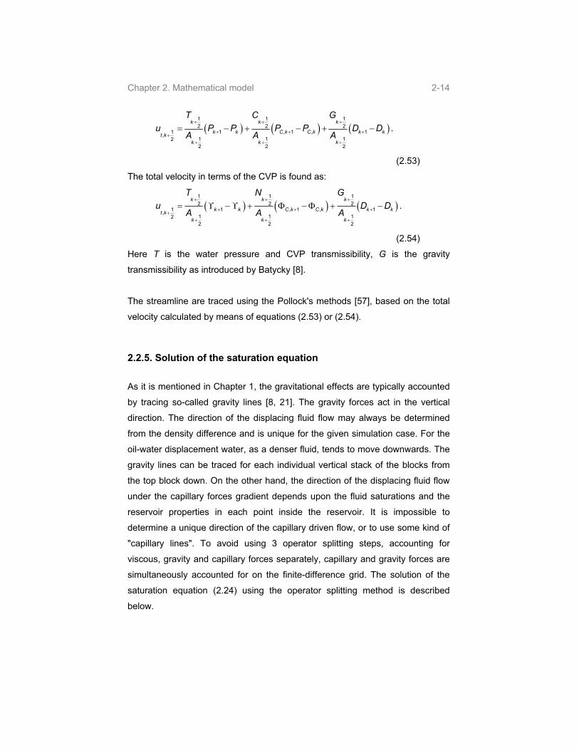
Chapter 2. Mathematical model 2-14
1 1 1
2 2 21 1 , 1 , 1
,1 1 12
2 2 2
k k k
k k C k C k k kt k
k k k
T C G
u P P P P DA A A
D .
(2.53)
The total velocity in terms of the CVP is found as:
1 1 1
2 2 21 1 , 1 , 1
,1 1 12
2 2 2
k k k
k k C k C k k kt k
k k k
T N G
u DA A A
D .
(2.54)
Here T is the water pressure and CVP transmissibility, G is the gravity
transmissibility as introduced by Batycky [8].
The streamline are traced using the Pollock's methods [57], based on the total
velocity calculated by means of equations (2.53) or (2.54).
2.2.5. Solution of the saturation equation
As it is mentioned in Chapter 1, the gravitational effects are typically accounted
by tracing so-called gravity lines [8, 21]. The gravity forces act in the vertical
direction. The direction of the displacing fluid flow may always be determined
from the density difference and is unique for the given simulation case. For the
oil-water displacement water, as a denser fluid, tends to move downwards. The
gravity lines can be traced for each individual vertical stack of the blocks from
the top block down. On the other hand, the direction of the displacing fluid flow
under the capillary forces gradient depends upon the fluid saturations and the
reservoir properties in each point inside the reservoir. It is impossible to
determine a unique direction of the capillary driven flow, or to use some kind of
"capillary lines". To avoid using 3 operator splitting steps, accounting for
viscous, gravity and capillary forces separately, capillary and gravity forces are
simultaneously accounted for on the finite-difference grid. The solution of the
saturation equation (2.24) using the operator splitting method is described
below.

Chapter 2. Mathematical model 2-15
The viscous forces are accounted for along the streamlines:
t
1
uww
sf
t0 . (2.55)
Using the time of flight concept, presented in Chapter 1 [18, 32, 68] equation
(2.55) is transformed from the three-dimensional Cartesian coordinates, to the
one-dimensional coordinate along the streamlines:
1
0w ws f
t, (2.56)
while gravitational and capillary effects are resolved on the finite-difference grid:
2
1 10w o o ww
c o w
t t
sk P k g D
t (2.57)
Equation (2.56) requires a single boundary condition, which is specified at the
injection well:
0 injecteds s . (2.58)
Solution of the equation (2.56) is described by Batycky [8]. After the equation
(2.56) is solved along the streamlines, the saturations are mapped back to the
finite-difference grid [8].
Equation (2.57) is solved explicitly on the finite difference grid. This step is
referenced as a corrector step, capable of relocating the fluids inside the porous
media, but not changing their total amounts. The simulation space for the
corrector step is bounded by the no-flow boundaries and does not contain any
source or sink terms. A first-order forward-in-time, backward-in-space finite-
difference scheme [55] is used. For simplicity the discretized form of the
equation (2.57) is shown in one dimension along the x-axis:
1
, , , 1 , , ,
1 2 1 22
1n n n n n n
w i w i c i c i c i c in n
i i
s s P P P PC C
t x x
1
2
11 2 1 22 2
10
n n n nn ni i i ii i
D D D DG G
x x
1 , (2.59)
here C and G are correspondingly capillary and gravity transmissibilities,
described in the previous section.

Chapter 2. Mathematical model 2-16
The three-dimensional discretization form contains y and z terms similar to
the x term in equation (2.59).
An important question arises during solution of the saturation equation (2.59)
when a displacement front (more generally, the capillary transition zone) moves
from one block to another. The multiplier of the capillary and gravity gradients,
equation (2.57) contains the w o
t
k term. For the reservoir simulation problems
the oil phase is immobile at the irreducible water saturation, as well as the water
phase is immobile at the residual oil saturation. Therefore the product of phase
mobilities is often close to zero in the block behind and the block ahead the
displacement front. For the solution procedures, based on the center-point
grids, used both in Eclipse and CapSL, this fact might create certain numerical
problems. Generally the transmissibility terms 1 2
n
iC and 1 2
n
iG can be found
using the i-th+1 block properties, the i-th block properties or by averaging the
w o tk values of these two blocks. As it is mentioned above, typically, the
harmonic averaging of the w o tk values in the neighboring blocks is used :
11 2
1
, , , 1 , 1
1
, ,
n i ii
i i
w i o i w i o i
i i
t i t i
k k1
, (2.60)
wherei is the distance from the i-th block center to the boundary.
And the capillary transmissibility is found as:
1 2 1 2
1 2
n
i
i
AC
x
n
i . (2.61)
If the mobility of any of the phases in any of the neighboring blocks approaches
zero, corresponding , ,i t i i w i o ik ,
approaches infinity, therefore the
1 2
n
i approaches zero. As a result, the IMPES Eclipse saturation step, and the
CapSL corrector step equation (2.59), have two requirements to be able to
redistribute fluids between two blocks with respect to capillary and gravitational
forces:
Chapter 2. Mathematical model 2-17
Both grid blocks must have the water saturation at least slightly higher
than initial water saturation. For the CapSL, this means that grid blocks
must be flooded during solution along the streamlines and for Eclipse,
that the blocks must be flooded by the viscous flow during the previous
time step.
Both grid blocks must have the oil saturation higher than residual oil
saturation. Therefore, if the water penetrates into the previously
unflooded grid block it should not fill it up to the maximum water
saturation during the single saturation time step.
Aziz and Settari [5] also state that for the multiphase flow the choice of the
averaging might be dictated by the numerical techniques used. In case of
capillary forces the harmonic averaging of the d
may not be the best choice,
since it may require time step smaller than IMPES stability condition, making
both simulators slower and more dispersed.
In reality, the displacement front represents a zone with a wide range of
saturations, and an average mobility in this zone highly differs from the
mobilities at its ends. An average mobility of oil and water in the capillary
transition zone corresponds to mobility at some average saturation between the
saturation values behind and ahead of the displacement front. For the sake of
simplicity, one may take an arithmetic average saturation:
1 11 2
1
i i i ii
i i
z s z ss
z z (2.62)
and to calculate the phase mobilities on the border corresponding to this
average saturation:
1 2 1 211 2
1 1 2
1
w i o in i ii
i i t i
i i
s s
s
k k
. (2.63)
To distinguish the methods further in the text the saturation equation solution
using equation (2.60) is called harmonic mean method. The saturation equation
solution using equation (2.63) is called average saturation method.

Chapter 2. Mathematical model 2-18
In many simple cases there is no difference between using the harmonic mean
and the average saturation method. However, in certain cases the latter method
should provide better simulation results. Comparison of the simulation results
obtained using these two methods is presented in Chapter 3.
The outline of the solution routine for the equation (2.59) is as follows:
1. Start with the first grid block;
2. Calculate capillary and gravity flux through all the faces of the grid block;
3. Calculate and save the water saturation change in the current block due
to all fluxes;
4. Repeat steps 2-3 for all the grid blocks;
5. Calculate the saturation values on the current time step using the
saturation on the previous step and the saved saturation change values.
The explicit solution scheme used for the corrector step is conditionally stable
[55] and requires limitation of the time step size [29]:
1i
pi
F t
V, (2.64)
where is the maximum stable time step, Vt p is the grid block pore volume and
F is some function of rates, reservoir and fluid properties.
Flux F is evaluated for each grid block as maximum total gravity and capillary
flux through any face of the block. The maximum stable time step is calculated
as:
, ,
1..6max
j C i j C i j i j i
jpi
C P P G D Dt
V, (2.65)
where index j represents one of the six faces of the grid block in the Cartesian
7-point stencil, index i represents the current grid block and index
represents the neighboring block through the face j.i j
In case of very strong capillary forces in a heterogeneous porous medium with
large permeability variation the corrector step may result in "overshoot" of the
saturation values in some grid blocks. That is the saturation in some specific
blocks become larger than 1-sor. Such an overshoot is the result of the explicit

Chapter 2. Mathematical model 2-19
treatment of the phase mobilities during a single corrector step. In this case the
corrector step is rejected and repeated with half the current time step.
2.2.6. Possibilities for the material balance error
Main sources of the numerical error in the black oil streamline simulator
accounting for the gravity and / or capillary effects are:
Mapping from finite-difference grid to streamlines and back;
The operator splitting error.
The numerical errors associated with mapping are described by Mallison et
al. [48]. Mallison et al. also suggest modifications to the mapping routine
allowing a significant decrease in the mapping error. It is easy to comprehend
that the mapping error increases with increase of the number of remappings
performed. This ultimately means that the mapping error increases with
increase of the number of time steps.
On the other hand, solution of the operator splitting method converges to the
analytical solution at infinitely large number of time steps. Strictly speaking it
should be possible to estimate the "optimal" number of time steps, where the
total numerical error is at minimum, as sketched on Figure 2-2.
Err
or
Nsteps
Mapping errorOperatorsplitting error
Figure 2-2. The mapping and the operator splitting errors.

Chapter 2. Mathematical model 2-20
2.2.7. Time step selection
The CapSL, in its current formulation, has several different time step types. The
first one is the pressure update time step, discussed here. The other two time
steps control the solution of the saturation equation. The time step t1 is
associated with solution of equation (2.56) along the streamlines. One-
dimensional explicit solution of the saturation equation along a given streamline
is restricted by the local CFL condition. Therefore, the time step along each
streamline is introduced [8]. The value of another time step - t2 is related to the
solution of the “corrector” step on the finite difference grid, equation (2.57) and
is discussed above. Equations (2.56) and (2.57) may be consecutively solved
several times for each pressure time step to correctly account for the cross flow
due to capillary and/or gravity forces. To avoid confusion between different time
steps of the streamline method the “time step” term is used with regard to the
pressure update time step. Each pressure update time step may include one or
more “saturation steps”. The “saturation step” term is used in regard to single
solution of the saturation equation, including both the solution along the
streamlines and on the finite difference grid. The stable saturation step size is
equal to the smallest of the step along the streamlines or on the finite difference
grid. Typically the gravity / capillary step on the finite difference grid is smaller
than the viscous step along the streamlines, therefore the saturation time step
size is limited by the stability condition of the corrector step, equation (2.57).
The size of the saturation step is determined using equation (2.66). Several
saturation steps might be performed during each time step. This allows
decreasing the operator splitting error of the saturation step without
recalculating the pressure field.
Selection of a stable time step size for the pressure update time step poses a
rather complicated problem. Compared to the finite-difference methods the
restrictions on the time step size of the streamline method are lifted mainly due
to complete decoupling of the pressure and the saturation update time steps [8].
Such decoupling is possible due to the movement of the fluids along the
streamlines. This leads to two advantages: 1) the solution of the saturation

Chapter 2. Mathematical model 2-21
equation is limited by the stability criteria along the particular streamline, not by
the largest flow velocity in the whole simulated domain; 2) the pressure
equation does not have to be recalculated every time the saturation equation is
solved.
Therefore the only remaining question about time step selection is the question
of convergence. In other words: how many pressure updates are necessary to
accurately capture non-linearity of the displacement?
Two different methods of the time step selection are available. The first one is
based on the user-specified output times. This method attempts to make the
time step as large as the user-specified saturation or pressure output times or
the well history specifications allow. The time step can be rejected if the mass
balance error is too large. Details of the mass balance error evaluation and the
time step rejection are provided below. The second time step selection routine
is based on the paper by Ichiro et al. [40]. The stability condition for the
streamline method is derived from the three-dimensional IMPES stability
condition [67]:
yxw
uu utCn f
x y zz , (2.66)
and for the streamline method the velocity in the stability condition is substituted
for the correction velocity, which is the difference between initial and
instantaneous velocity at the current step. It is assumed that the change in the
volumetric flux through the block face is proportional to the time step size and
for each block it may be found as:
0 maxW
wf
Sinflow w
ftCn q q
PV s, (2.67)
here Cn is the Courant number: the dimensionless number allowing to take the
time steps smaller or larger than the stable time step [29]; t is the time step;
PV is the pore volume of the block; qf is the volumetric flux after the time step;
q0 is the volumetric flux before the time step. On the basis of the equation (2.67)
the size of the next time step may be estimated from the maximum change of
the velocity during the current step. The method suggested is used to estimate
the size of the next time step, based on the size of the current time step and the

Chapter 2. Mathematical model 2-22
flow velocity change. The method described above provides a quick, CPU-
cheap and efficient solution to estimate the time step size.
A better time step selection algorithm may probably be obtained by following the
method suggested by Coats [28]. This method is obtained for the finite-
difference IMPES solution and should be re-evaluated for the streamline
method.
After the time step is performed the mass balance error is evaluated:
. (2.68) , , ,
1 1
steps stepsn n
water initial water injected water produced water in place
i i
E V V V V ,
Here V is volume and nsteps is the number of time steps performed.
If the mass balance error exceeds the user-specified value, the step may be
rejected and repeated with, for example, half the current time step size.
Originally in 3DSL Batycky [8] suggested another method, the so-called "true
time". The underlying idea is to find a "true" time step size from the cumulative
water balance on the given time step, see Section 1.3.3. As a result the mass
balance error is "converted" into the time step size error. However, the
streamline simulator is based on the numerical approximations, rather than on
the exact analytical solutions. Any approximation and therefore any numerical
method have an error associated with it. Two main sources of the numerical
error in the streamline simulation are mentioned above. A numerical error is as
important parameter as the solution speed. It is important not only to compare
how fast the numerical simulation delivers the predictions, but how fast the
numerical simulation delivers the predictions within the certain level of accuracy.
It should also be mentioned that for the viscous dominated simulation runs the
mass balance error is typically very small and the time steps are rather large.
As a result the correction to the time step size does not have any serious effects
on the simulation times.
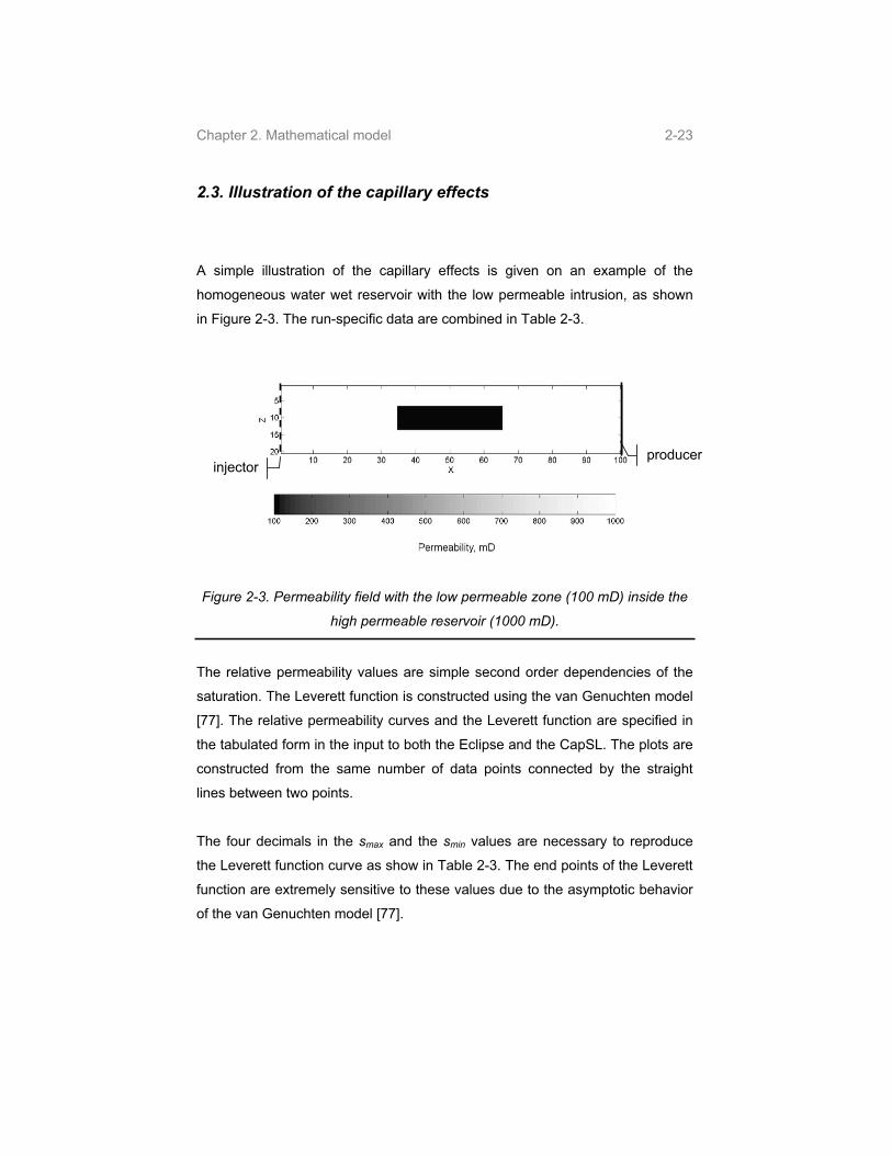
Chapter 2. Mathematical model 2-23
2.3. Illustration of the capillary effects
A simple illustration of the capillary effects is given on an example of the
homogeneous water wet reservoir with the low permeable intrusion, as shown
in Figure 2-3. The run-specific data are combined in Table 2-3.
producerinjector
Figure 2-3. Permeability field with the low permeable zone (100 mD) inside the
high permeable reservoir (1000 mD).
The relative permeability values are simple second order dependencies of the
saturation. The Leverett function is constructed using the van Genuchten model
[77]. The relative permeability curves and the Leverett function are specified in
the tabulated form in the input to both the Eclipse and the CapSL. The plots are
constructed from the same number of data points connected by the straight
lines between two points.
The four decimals in the smax and the smin values are necessary to reproduce
the Leverett function curve as show in Table 2-3. The end points of the Leverett
function are extremely sensitive to these values due to the asymptotic behavior
of the van Genuchten model [77].
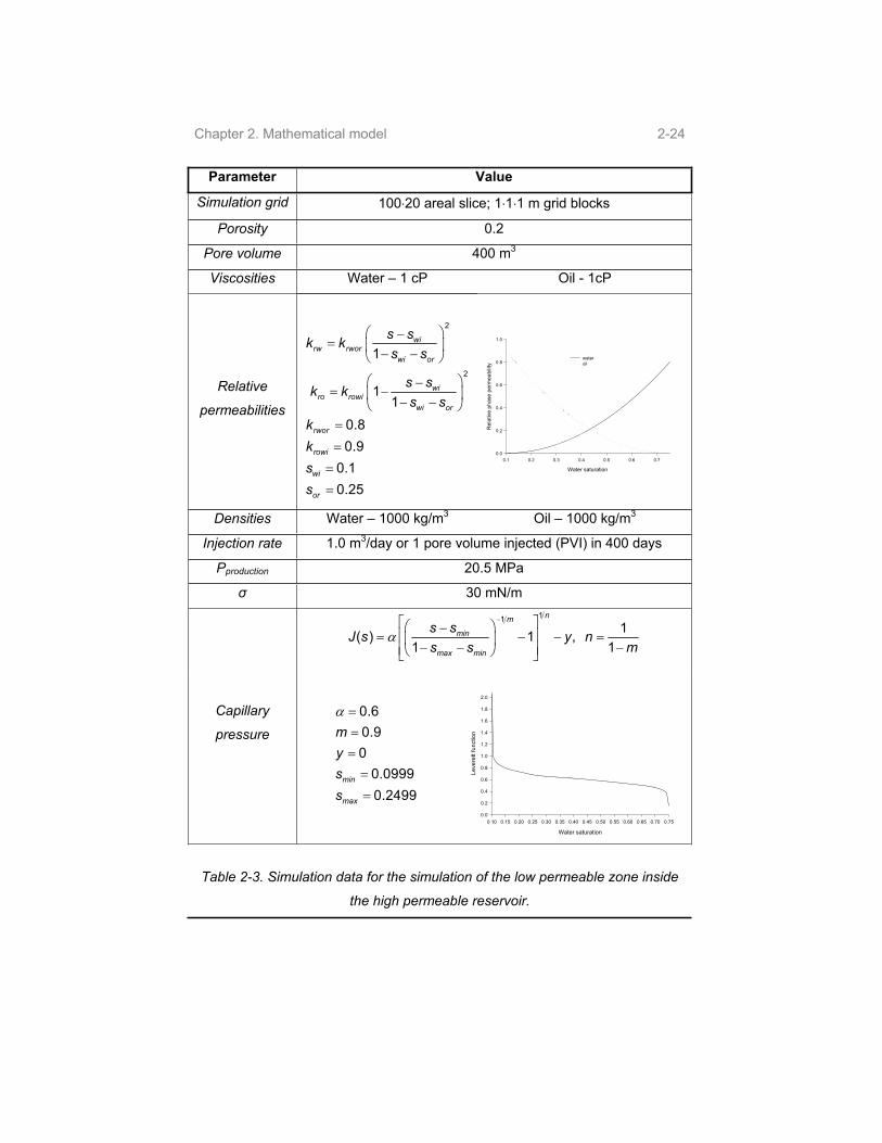
Chapter 2. Mathematical model 2-24
Parameter Value
Simulation grid 100 20 areal slice; 1 1 1 m grid blocks
Porosity 0.2
Pore volume 400 m3
Viscosities Water – 1 cP Oil - 1cP
Relative
permeabilities
2
2
1
11
0.8
0.9
0.1
0.25
wirw rwor
wi or
wiro rowi
wi or
rwor
rowi
wi
or
s sk k
s s
s sk k
s s
k
k
s
sR
ela
tive
ph
ase
pe
rmea
bili
ty
0.1 0.2 0.3 0.4 0.5 0.6 0.7
Water saturation
0.0
0.2
0.4
0.6
0.8
1.0
water
oil
Densities Water – 1000 kg/m3 Oil – 1000 kg/m3
Injection rate 1.0 m3/day or 1 pore volume injected (PVI) in 400 days
Pproduction 20.5 MPa
30 mN/m
11
1( ) 1 ,
1 1
nm
min
max min
s sJ s y n
s s m
Capillary
pressure
0.6
0.9
0
0.0999min
m
y
s
0.2499maxs
Water saturation
0.10 0.15 0.20 0.25 0.30 0.35 0.40 0.45 0.50 0.55 0.60 0.65 0.70 0.75
Le
vere
tt fu
nction
0.0
0.2
0.4
0.6
0.8
1.0
1.2
1.4
1.6
1.8
2.0
Table 2-3. Simulation data for the simulation of the low permeable zone inside
the high permeable reservoir.

Chapter 2. Mathematical model 2-25
The displacement fronts neglecting capillary effects are presented in Figure 2-4.
0.3 PVI 0.5 PVI
Water saturation
Figure 2-4. Saturation profiles for the low permeable zone inside the high
permeable reservoir simulation without accounting for capillary forces.
Two zones are highlighted in Figure 2-4. The solid line surrounds the low
permeable zone, the dashed line surrounds the high permeable zone after
(corresponding to the direction of the flow) the low permeable zone. These two
zones are of the particular interest, since capillary effects are expected to
strongly alter the saturation displacement front in these two zones. Figure 2-5
shows the saturation profiles at the same PVI, obtained by the CapSL utilizing
the SFD pressure equation modification without accounting for capillary effects
in the saturation equation. Figure 2-6 shows the corresponding saturation
profiles obtained by the CapSL utilizing the CVP equation without accounting for
capillary effects in the saturation equation.
The SFD and the CVP saturation profiles are quite different. The permeability
field is symmetric with respect to the horizontal line passing through the middle
of it. Therefore the saturation profiles must be symmetric with respect to this line
as well. However, the SFD method shows an asymmetry in the saturation
profiles.
The increase in the simulation time with capillary effects is below 5% for both
methods. This time comparison is preliminary, the detailed information on
comparison of the methods is presented in Chapter 3.

Chapter 2. Mathematical model 2-26
0.3 PVI 0.5PVI
Water saturation
Figure 2-5. Saturation profiles for the low permeable zone inside the high
permeable reservoir simulation obtained by the CapSL utilizing the SFD method
without accounting for capillary effects in the saturation equation.
0.3 PVI 0.5PVI
Water saturation
Figure 2-6. Saturation profiles for the low permeable zone inside the high
permeable reservoir simulation obtained by the CapSL utilizing the CVP method
without accounting for capillary effects in the saturation equation.
As it can be seen from the comparison of Figures 2-5 and 2-6 with Figure 2-4,
two main effects of the capillary forces are:
Higher sweep of the low permeable zone;
Smearing of the displacement front, resulting in the faster sweep of the
high permeable area after the low permeable zone.

Chapter 2. Mathematical model 2-27
The smearing of the saturation front is achieved only due to the change in the
total velocity and the location of the streamlines as a result of accounting for the
capillary forces in the pressure equation.
The simulation results accounting for the capillary forces both in the pressure
and the saturation equations are presented in Figure 2-7.
Straightforward method
0.3 PVI 0.5PVI
Capillary-Viscous Potential
0.3 PVI 0.5PVI
Water saturation
Figure 2-7. Saturation profiles for the low permeable zone inside the high
permeable reservoir simulation accounting for capillary forces in the pressure
and the saturation equations.
Simulations using the CVP and the SFD methods show a good match.

Chapter 2. Mathematical model 2-28
Introduction of the capillary effects results in a higher water saturation in the low
permeable zone and in smearing of the displacement front. With the capillary
effects accounted for both in the pressure and the saturation equations, the
average water saturation in the low permeable zone after 0.5 PVI injected has
increased approximately twice: from 0.30 to 0.61 compared to the simulation
neglecting the capillary forces.
The cumulative oil production curves for 1) simulation neglecting capillary
effects; 2) using the CVP method neglecting the capillary effects in the
saturation equation; and 3) accounting for capillary effects both in the pressure
and the saturation equations are compared on Figure 2-8.
Pore volumes of water injected
0.0 0.5 1.0 1.5 2.0
Pore
volu
mes o
f oil
pro
du
ced
0.0
0.1
0.2
0.3
0.4
0.5
0.6
0.7
No capillary effects
Capillary effects accounted for only in the pressure equation
Capillary effects accounted for both in the pressure and the saturation equations
Figure 2-8. Oil production curves for the low permeable zone inside the high
permeable reservoir simulation.
The breakthrough occurs at around 0.54 PVI if the capillary effects are
neglected, at around 0.5 PVI if the capillary effects are accounted for only in the
pressure equation and at 0.53 PVI if the capillary effects are fully accounted for.
A faster breakthrough time can be explained by smearing of the saturation front
due to the capillary forces. Slowing down the front with respect to the
modification of the saturation equation is due to increase of the capillary cross
flow.

Chapter 2. Mathematical model 2-29
Comparison of the CapSL (accounting for capillary effects both in the pressure
and the saturation equations) and the Eclipse 100 (IMPES mode) predictions
after 0.3 and 0.5 PVI, Figures 2-9 and 2-10, respectively, shows that the CapSL
predictions result in weaker capillary crossflow.
Figure 2-9. Comparison of the Eclipse and the CapSL saturation plots for the
low permeable zone inside the high permeable reservoir simulation after 0.3
PVI.
Figure 2-10. Comparison of the Eclipse and the CapSL saturation plots for the
low permeable zone inside the high permeable reservoir simulation after 0.5
PVI.
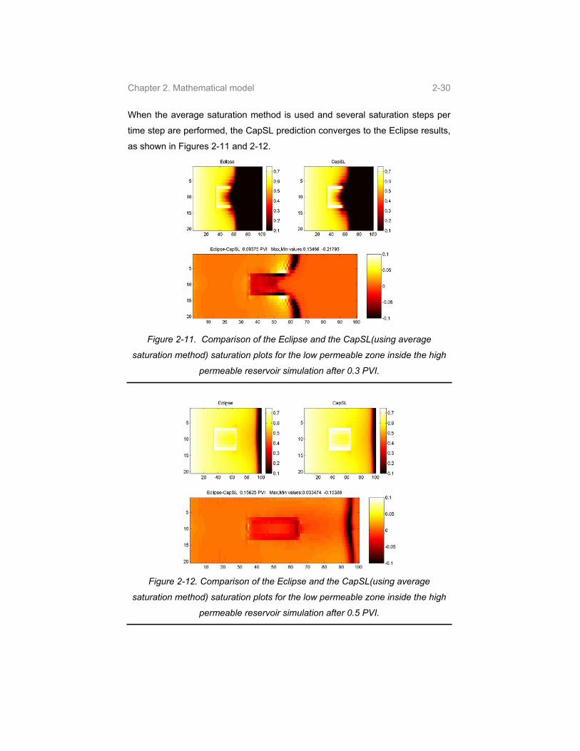
Chapter 2. Mathematical model 2-30
When the average saturation method is used and several saturation steps per
time step are performed, the CapSL prediction converges to the Eclipse results,
as shown in Figures 2-11 and 2-12.
Figure 2-11. Comparison of the Eclipse and the CapSL(using average
saturation method) saturation plots for the low permeable zone inside the high
permeable reservoir simulation after 0.3 PVI.
Figure 2-12. Comparison of the Eclipse and the CapSL(using average
saturation method) saturation plots for the low permeable zone inside the high
permeable reservoir simulation after 0.5 PVI.

Chapter 2. Mathematical model 2-31
However, even in this case the capillary crossflow in the CapSL predictions is
slightly lower compared to the Eclipse. One of the possible explanations may be
higher numerical dispersion in the Eclipse.
Finally, the comparison of the cumulative oil production curves using the CVP
with different saturation equation modifications and the Eclipse 100 is presented
in Figure 2-13.
Pore volumes of water injected
0.5 1.0 1.5 2.0
Po
re v
olu
me
s o
f o
il p
rod
uce
d
0.45
0.50
0.55
0.60
0.65
CVP equation with harmonic averaging of the transmissibilities
CVP equation with average saturation
Eclipse
Figure 2-13. Oil production curves predicted by the Eclipse and the CapSL for
the low permeable zone inside the high permeable reservoir simulation.
The oil production curves predicted by the CapSL using the average saturation
method by the Eclipse show not only a good match in general, but show similar
trends.
The maximum mass balance error of the streamline simulator in all the
simulations mentioned above remains below 0.2% relative to the pore volume.
The next chapter will present more simulation examples. The CapSL simulator
will be tested on the synthetic cases and compared to the Eclipse.


3-1
Chapter 3. Comparison of various methods of
accounting for capillary effects
The chapter starts with a comparison of the various modification methods
described in Chapter 2. Several test cases are presented. The capillary-viscous
potential method (CVP) and the straightforward method of introduction of
capillary effects into the pressure equation (SFD) are compared first. The
saturation equation modifications are discussed. The time step methods are
tested.
It is very difficult to compare only the modifications of the pressure equation or
only the time step selection routine. A comparison of the CVP and the SFD
methods without the time step selection routine and the saturation equation
modification is not entirely correct and complete. Introduction of the capillary
effects into the pressure equation influences the initial condition of the
saturation step by altering the streamline locations. The stability of the modified
scheme may restrict or ease up the time steps size limitation. The introduction
of capillary effects into the saturation equation influences the pressure equation
solution on the next time step through the capillary pressure term. The time step
size determines how many local steps along the streamlines and on the finite-
difference grid are required due to the CFL (Courant-Freidrich-Levi [76]) stability
condition [19, 20] during the single pressure update time step. An attempt is
carried out to separately analyze the effects of introduction of capillary effects
into the pressure and the saturation equations and the automatic time step size
selection routine. However, a lot of cross influence is discovered and discussed.
3.1. Data for the test cases
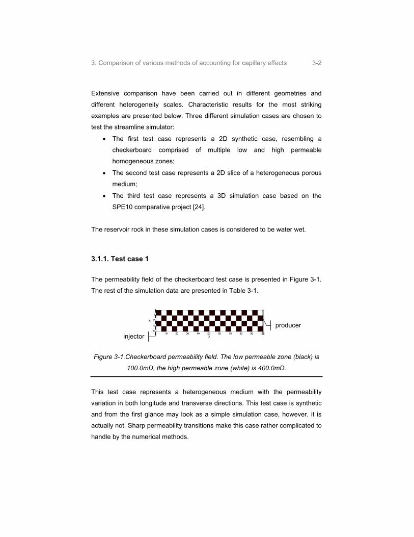
3. Comparison of various methods of accounting for capillary effects 3-2
Extensive comparison have been carried out in different geometries and
different heterogeneity scales. Characteristic results for the most striking
examples are presented below. Three different simulation cases are chosen to
test the streamline simulator:
The first test case represents a 2D synthetic case, resembling a
checkerboard comprised of multiple low and high permeable
homogeneous zones;
The second test case represents a 2D slice of a heterogeneous porous
medium;
The third test case represents a 3D simulation case based on the
SPE10 comparative project [24].
The reservoir rock in these simulation cases is considered to be water wet.
3.1.1. Test case 1
The permeability field of the checkerboard test case is presented in Figure 3-1.
The rest of the simulation data are presented in Table 3-1.
injector
producer
Figure 3-1.Checkerboard permeability field. The low permeable zone (black) is
100.0mD, the high permeable zone (white) is 400.0mD.
This test case represents a heterogeneous medium with the permeability
variation in both longitude and transverse directions. This test case is synthetic
and from the first glance may look as a simple simulation case, however, it is
actually not. Sharp permeability transitions make this case rather complicated to
handle by the numerical methods.

3. Comparison of various methods of accounting for capillary effects 3-3
Parameter Value
Grid 100 20 1m areal slice; Each checker-block is 5 5m
Porosity 0.2
Pore volume 400 m3
Viscosities Water – 1 cP Oil - 1cP
Relative
permeabilities
2
2
1
11
0.8
0.9
0.1
0.25
wirw rwor
wi or
wiro rowi
wi or
rwor
rowi
wi
or
s sk k
s s
s sk k
s s
k
k
s
s
Rea
ltive
per
mea
bilit
y0.10 0.15 0.20 0.25 0.30 0.35 0.40 0.45 0.50 0.55 0.60 0.65 0.70 0.75
Water saturation
0.0
0.1
0.2
0.3
0.4
0.5
0.6
0.7
0.8
0.9
1.0
Relative permeability to waterRelative permeability to oil
Densities Water – 1000 kg/m3 Oil – 1000 kg/m3
Injection rate 1.0 m3/day (1 pore volume injected in 400 days)
Pproduction 20.5 MPa
30 mN/m
111
( ) 1 , 1 1
nm
min
max min
s sJ s y n
s s m
Capillary
pressure
0.5
0.93
0.05
0.0999min
m
y
s
0.75maxs
Water saturation
0.1 0.2 0.3 0.4 0.5 0.6 0.7
Leve
rett
func
tion
0.0
0.2
0.4
0.6
0.8
1.0
1.2
Table 3-1. Simulation data for checkerboard case.

3. Comparison of various methods of accounting for capillary effects 3-4
3.1.2. Test case 2
The second test case is similar to the one used by Thiele [70]. This test case
represents a two-dimensional slice of a heterogeneous medium. The porosity of
the medium is kept constant; however, the permeability varies from 273mD to
135D. The average permeability value is 9D. The permeability field is
constructed using log-normal distribution and is presented in Figure 3-2. The
simulation data are presented in Table 3-2.
injector producer
Figure 3-2. Second test case. Permeability field.
The fluid viscosities are based on the data from the SPE fifth comparative
project [45].

3. Comparison of various methods of accounting for capillary effects 3-5
Parameter Value
Grid 124 50 areal slice; 406.72 3.28 164 m reservoir
Porosity 0.2
Pore volume 43756.56 m3
Viscosities Water – 0.25 cP Oil – 0.40 cP
Relative
permeabilities
2
2
1
11
0.8
0.9
0.1
0.2
wirw rwor
wi or
wiro rowi
wi or
rwor
rowi
wi
or
s sk k
s s
s sk k
s s
k
k
s
sWater saturation
0.1 0.2 0.3 0.4 0.5 0.6 0.7 0.8
Rel
ativ
e pe
rmea
bilit
y
0.0
0.1
0.2
0.3
0.4
0.5
0.6
0.7
0.8
0.9
1.0
Water relative permeabilityOil relative permeability
Densities Water – 1000 kg/m3 Oil – 1000kg/m3
Injection rate 43.79 m3/day (1 pore volume injected in about 1000 days)
Pproduction 11.03 MPa
30 mN/m
111
( ) 1 , 1 1
nm
min
max min
s sJ s y n
s s m
Capillary
pressure
0.6
0.9
0
0.09999min
m
y
s
0.801maxs
Water saturation
0.10 0.15 0.20 0.25 0.30 0.35 0.40 0.45 0.50 0.55 0.60 0.65 0.70 0.75 0.80
Leve
rett
func
tion
0.0
0.2
0.4
0.6
0.8
1.0
1.2
1.4
1.6
1.8
2.0
Table 3-2. Second test case. Simulation data.

3. Comparison of various methods of accounting for capillary effects 3-6
3.1.3. Test case 3
The third test case is the upscaled grid from the 10th SPE reservoir comparative
project [24]. The porosity field is presented in Figure 3-3. The permeability
varies around 7 orders of magnitude from 0.007 to 3565mD with an average of
53.8mD and is presented in common logarithm scale in Figure 3-4. The
simulation data is gathered in Table 3-3.
Injector
Producer
Figure 3-3. The third test case. The porosity field.
Figure 3-4. Thr third test case. The permeability field in common logarithmic
scale.

3. Comparison of various methods of accounting for capillary effects 3-7
Parameter Value
Grid 60 100 8; 6.0 6.0 6.5 m grid blocks
Pore volume 2'108'569 m3
Viscosities Water – 0.4 cP Oil – 0.25 cP
Relative
permeabilities
2
2
1
11
0.8
0.9
0.1
0.25
wirw rwor
wi or
wiro rowi
wi or
rwor
rowi
wi
or
s sk k
s s
s sk k
s s
k
k
s
s
Rel
ativ
e ph
ase
perm
eabi
lity
0.1 0.2 0.3 0.4 0.5 0.6 0.7
Water saturation
0.0
0.2
0.4
0.6
0.8
1.0
wateroil
Densities Water – 1000 kg/m3 Oil – 1000 kg/m3
Injection rate 2 injectors 1084.474m3/day each
Pproduction 6 producers at 30 MPa BHP
30 mN/m
111
( ) 1 , 1 1
nm
min
max min
s sJ s y n
s s m
Capillary
pressure
0.6
0.9
0.017
m
y
0.0999
0.800001min
max
s
s
Water saturation
0.1 0.2 0.3 0.4 0.5 0.6 0.7 0.8
Leve
rtt f
unct
ion
0.00.10.20.30.40.50.60.70.80.91.01.11.21.31.41.51.61.71.81.92.02.1
Table 3-3. Third test case. Simulation data.
The 6 decimals in the smax value are necessary to reproduce the Leverett
function curve as show in Table 3-3. The end points of the Leverett function are

3. Comparison of various methods of accounting for capillary effects 3-8
extremely sensitive to these values due to the asymptotic behavior of the van
Genuchten model [77]. For example, at a water saturation of 0.8 the Leverett
function has the value of 0.141 when smax equal to 0.800001. If the smax is
changed to 0.801, the Leverett function at sw=0.8 increases by more than a
factor of two to the value of 0.297.
3.2. Estimation of the displacement regime
The governing equations (2.24) and (2.25) may be transformed to a
dimensionless form. For this purpose a set of the dimensionless groups is
introduced. Using these groups the relative magnitude of the capillary, gravity
and viscous forces may be determined. The approach of making the equations
dimensionless is given by, for example, Bedrikovetsky [9] and Zhou et al. [80]
and is in general similar. However, the details may differ and as a result several
sets of the dimensionless groups are derived. These groups may be applied for
two different purposes:
Estimate the displacement regime to choose the optimum simulation
tools and simulation options;
Estimate if the simulation results do make sense from the point of view of
the physics of the fluid flow in porous media.
The estimation of the displacement regime is carried out using two groups of
the dimensionless parameters. The first set is presented by Bedrikovetsky [9].
The dimensionless parameters include the capillary-viscous ratio:
10
cosrowi av avk k
U L, (3.1)
The anisotropy ratio:2
2 2x
z
H k
L k, (3.2)
and the capillary-gravity ratio:

3. Comparison of various methods of accounting for capillary effects 3-9
3cos
w o
av av
gH
k. (3.3)
Here krowi is the end point oil relative permeability, index i represents the
average properties, L is the characteristic length, U is the linear velocity, kav is
the average field permeability, av is the average field porosity.
The displacement regimes are classified according to Table 3-4.
Dimensionless parameters Displacement regime
11 2 31; 1 Viscous Dominant
11 2 31; 1 Vertical Equilibrium
11 2 31; 1 Capillary Dominant
11 2 31; 1 Gravity Dominant
2 1 Commingled Layers
Table 3-4. Determination of the displacement regimes by means of
Bedrikovetsky dimensionless groups.
Zhou et al. [80] derived different set of dimensionless parameters.
The gravity to viscous ratio is estimated as:
avgv
o
gLkN
Hq, (3.4)
The capillary to viscous ratio as: *
2c av
cv
o
LP kN
H q , (3.5)
here q is the flow rate, is the characteristic transverse capillary pressure of
the medium:
*cP
1*
1
or
wi
s
c w
c
or wis
P sP
s sds , (3.6)

3. Comparison of various methods of accounting for capillary effects 3-10
here sw is the water saturation, sor is the residual oil saturation and swi is the
initial water saturation.
Introducing the capillary pressure, equation (1.17) into equation (3.6):
1*
cos
1
or
wi
ws
c
or wis
J sk
Ps s
ds , (3.7)
and regrouping the variables:
1* cos
1
or
wi
s
c
sor wi
Pk s s
wJ s ds . (3.8)
The mobility ratio is introduced as:
w
o
M , (3.9)
and the shape factor as: 2
22
zl
x
L kR
H k. (3.10)
The displacement regime may be determined using Table 3-5.
Dimensionless parameters Displacement regime
1.01
gv cvN N M
MViscous Dominant
21.0; 1.01
gv cv
l
N N MR
MVertical Equilibrium
; 1.01
cvgv cv
MNN N
MCapillary Dominant
; 1.01
gv
gv cv
MNN N
MGravity Dominant
; 1.01
cvgv cv
MNN N
MCapillary-Gravity Equilibrium
21.0; 1.01
gv cv
l
N N MR
MCommingled Layers
Table 3-5. Determination of the displacement regimes by means of Zhou et
al. dimensionless groups.

3. Comparison of various methods of accounting for capillary effects 3-11
3.3. Comparison of the pressure equation modifications
First the CVP and the SFD methods of accounting for capillary effects in the
pressure equation are compared on the test case 1 without the saturation
equation modification and without any kind of automatic time step selection
routine. The effects of the grid refinement and the number of time steps on the
simulation time and the material balance error of both methods are investigated.
Later the CVP and the CFD methods are compared with inclusion of the
capillary effects in the saturation equation.
Three different grid sizes are used in this test:
The coarse grid comprised of 20 4 grid blocks. Each checker block is
represented by just one block;
The medium size grid comprised of 100 20 grid blocks. Each checker
block is represented by 5 blocks in each direction (25 in total);
The fine scale grid comprised of 500 100 grid blocks. Each checker block
is represented by 25 blocks in each direction (625 in total).
Each run simulates 800 days or 2 PV of water injection using 20 time steps. The
comparison is performed based on the oil production curves and the
displacement profiles, that is to say on the production history.
The comparison of the CPU time and the maximum mass balance error is
performed for the following runs: 1) neglecting capillary effects; 2) using the
SFD method of introduction of capillary effects into the pressure equation; 3)
using the CVP method. The SFD and the CVP simulation runs are performed
neglecting the capillary effects in the saturation equation.
The methods of both Bedrikovetsky and Zhou et al. indicate the capillary
dominated displacement, as shown in Table 3-6.

3. Comparison of various methods of accounting for capillary effects 3-12
Dimensionless parameters Value
11 2 34.78
3 0
Displacement regime Capillary Dominant
Bedrikovets
ky
1cvMN M 1.63
gvN 0
cvN 3.27
Zh
ou
et
al.
Displacement regime Capillary Dominant
Table 3-6. Determination of the displacement regimes. Checkerboard case.
The simulation without capillary effects is tested first. The oil production curves
for three different grids are shown in Figure 3-5.
Pore volumes of water injected
0.0 0.5 1.0 1.5 2.0
Por
e vo
lum
es o
f oil
prod
uced
0.0
0.1
0.2
0.3
0.4
0.5
0.6
0.7
Fine gridMedium gridCoarse grid
Figure 3-5.The checker board case. Oil production for the simulation without
capillary effects on different simulation grids.
The oil production curves show the volume of oil produced as a function of the
volume of water injected. For the immiscible incompressible case before the
breakthrough the volume of oil produced is equal to the volume of water
injected, indicated by the straight line on Figure 3-5. However, after the
breakthrough the production well produces the water-oil mixture, rather than just
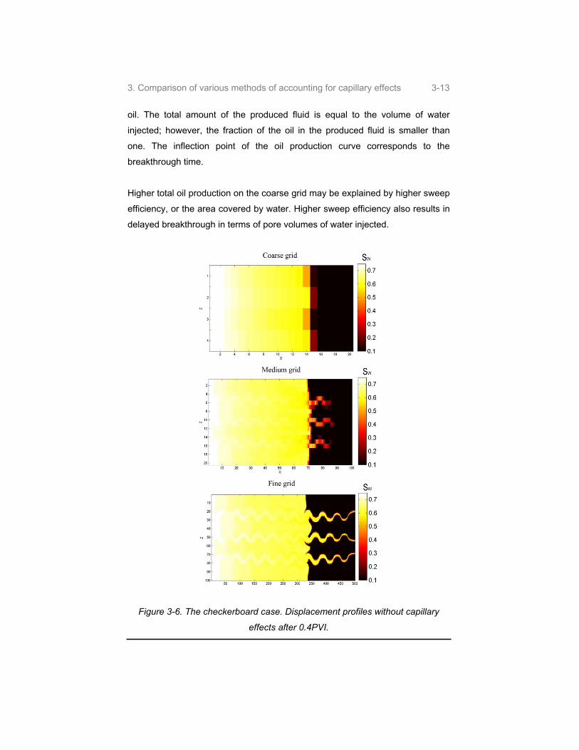
3. Comparison of various methods of accounting for capillary effects 3-13
oil. The total amount of the produced fluid is equal to the volume of water
injected; however, the fraction of the oil in the produced fluid is smaller than
one. The inflection point of the oil production curve corresponds to the
breakthrough time.
Higher total oil production on the coarse grid may be explained by higher sweep
efficiency, or the area covered by water. Higher sweep efficiency also results in
delayed breakthrough in terms of pore volumes of water injected.
Figure 3-6. The checkerboard case. Displacement profiles without capillary
effects after 0.4PVI.

3. Comparison of various methods of accounting for capillary effects 3-14
In the fine grid simulation it is possible to observe the fingering of water inside
the water saturated region (white fingers inside the yellow region in Figure 3-6).
In retrospect the fingers inside the water saturated zone are practically invisible
in the medium grid – the fingering of water is only indicated in the oil saturated
media (yellow fingers inside the black region in Figure 3-6). In the coarse grid
the fingering is captured only by the difference in the saturation of the
neighboring blocks around the saturation front.
The difference in the breakthrough time is due to the fingering of the water
through the high permeable checkers. The coarse model fails to capture these
effects, as shown in Figure 3-6.
The oil production curves for the simulations using the CVP and the SFD
methods are shown in Figure 3-7. The oil production curves are shown starting
from 0.5 PVI to highlight the difference in the oil production curves after the
breakthrough.
Pore volumes of water injected
0.5 1.0 1.5 2.0
Por
e vo
lum
es o
f oil
prod
uced
0.5
0.6
0.7
CVP on the fine gridSFD on the fine gridCVP on the coarse gridSFD on the coarse gridCVP on medium gridSFD on medium grid
Figure 3-7. The checkerboard case. Oil production for the simulation on
different grids sizes with capillary effects introduced only in the pressure
equation.

3. Comparison of various methods of accounting for capillary effects 3-15
The CVP modification method shows a small difference in the oil production
curves on the medium and the fine grids compared to the SFD method.
Behavior of the oil production curves simulated using the SFD modification is
similar to simulation without capillary effects.
Introduction of capillary effects into the pressure equation only is not sufficient
to completely remove the fingering of water; however, the water saturation in
the fingers decreases, as shown in Figure 3-8. The SFD method pulls back the
fingers to a larger extent, comparing to the CVP method. However, the SFD
method shows more numerical problems in the water saturated zone.
Figure 3-8. The checkerboard case. Displacement profiles at 0.4 PVI.
All simulations show increase of the CPU time required with increase of the grid
size. The CVP method is the fastest on all the three grids. The simulation times
versus the grid size are plotted in Figure 3-9. Speed ups of the simulation time
with the CVP method compared to the simulation without capillary effects and
the SFD method may be due to the reformulation of the pressure equation. The
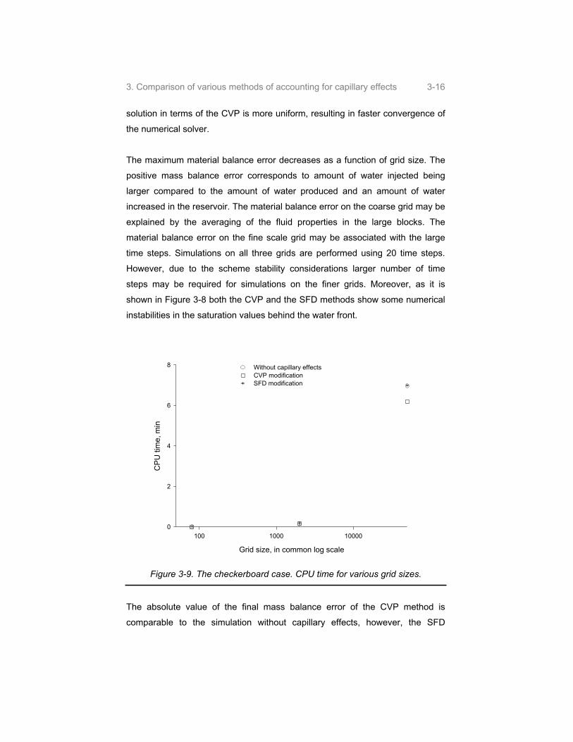
3. Comparison of various methods of accounting for capillary effects 3-16
solution in terms of the CVP is more uniform, resulting in faster convergence of
the numerical solver.
The maximum material balance error decreases as a function of grid size. The
positive mass balance error corresponds to amount of water injected being
larger compared to the amount of water produced and an amount of water
increased in the reservoir. The material balance error on the coarse grid may be
explained by the averaging of the fluid properties in the large blocks. The
material balance error on the fine scale grid may be associated with the large
time steps. Simulations on all three grids are performed using 20 time steps.
However, due to the scheme stability considerations larger number of time
steps may be required for simulations on the finer grids. Moreover, as it is
shown in Figure 3-8 both the CVP and the SFD methods show some numerical
instabilities in the saturation values behind the water front.
Grid size, in common log scale
100 1000 10000
CP
U ti
me,
min
0
2
4
6
8 Without capillary effectsCVP modificationSFD modification
Figure 3-9. The checkerboard case. CPU time for various grid sizes.
The absolute value of the final mass balance error of the CVP method is
comparable to the simulation without capillary effects, however, the SFD

3. Comparison of various methods of accounting for capillary effects 3-17
modification results in higher, in absolute values, mass balance error, as shown
in Figure 3-10.
Grid size, in common log scale
100 1000 10000
Max
imum
mas
s ba
llanc
e er
ror,
% o
f PV
-1.5
-1.0
-0.5
0.0
0.5
Without capillary effectsCVP modificationSFD modification
Figure 3-10. The checkerboard case. Maximum mass balance error for various
grid sizes.
Since the medium grid captures the main features of the flow and the simulation
times are significantly shorter comparing to the fine grid, the influence of the
number of time steps is investigated on the medium grid.
Influence of the number of time steps on the total CPU time requirement is
rather small, as shown in Figure 3-11.

3. Comparison of various methods of accounting for capillary effects 3-18
Number of pressure updates
0 10 20 30 4
CP
U ti
me,
min
00.15
0.16
0.17
0.18
0.19
0.20
0.21
0.22SFD methodCVP method
Figure 3-11. The checkerboard case. CPU time for various number of pressure
updates.
When the number of time steps increases 8 times (from 5 to 40), the CPU time
only increases about 35%.
Tracing the streamlines with respect to the capillary pressure should lift up the
restriction on the time step size associated with the capillary non-linearities in
the similar way as it does for the non-linearities associated with mobilities, see
Section 2.2.7. Therefore the CPU time may be restricted only by the numerical
solver. The pressure solutions for the small time step sizes converge faster,
compensating for the larger number of the solutions required.
The material balance error does not show any significant dependency on the
time step size. It decreases in absolute value for the SFD modification method,
however, the CVP method shows smaller mass balance error for any number of
time steps taken, as shown in Figure 3-12.

3. Comparison of various methods of accounting for capillary effects 3-19
Number of time steps
0 10 20 30 4
Max
imum
mas
s ba
llanc
e er
ror
0
-1.0
-0.8
-0.6
-0.4
-0.2
0.0
0.2
CVPSFD
Figure 3-12. The checkerboard case. Maximum mass balance error for various
number of time steps.
The number of time steps has quite a pronounced effect on the oil production
curves. It may be concluded from Figure 3-13 that 20 time steps provide
sufficient quality of the solution.
The oil production curves, starting from 0.5PVI for different numbers of time
steps are shown in Figure 3-13.
Based on the simulations presented above, it may be concluded that the CVP
method delivers smaller mass balance error. However, both modification
methods should be further compared with full account for capillary effects.

3. Comparison of various methods of accounting for capillary effects 3-20
Pore Volumes of Water Injected
0.6 0.8 1.0 1.2 1.4 1.6 1.8 2.0
Por
e V
olum
es o
f Oil
prod
uced
0.5
0.6
0.7
0.8
0.9 CVP 5 stepsCVP 10 stepsCVP 20 stepsCVP 40 stepsSFD 5 stepsSFD 10 stepsSFD 20 stepsSFD 40 steps
Figure 3-13. The checkerboard case. Oil production curves for the simulations
using different number of time steps, with capillary effects introduced only in the
pressure equation.
The simulation accounting for capillary effects both in the pressure and the
saturation equations is performed using 20 time steps. Harmonic averaging of
the transmissibilities in the saturation corrector step is used. Comparison of the
saturation fronts obtained with the CVP and the SFD methods after 0.3 and 0.5
PVI are presented in Figures 3-14 and 3-15.
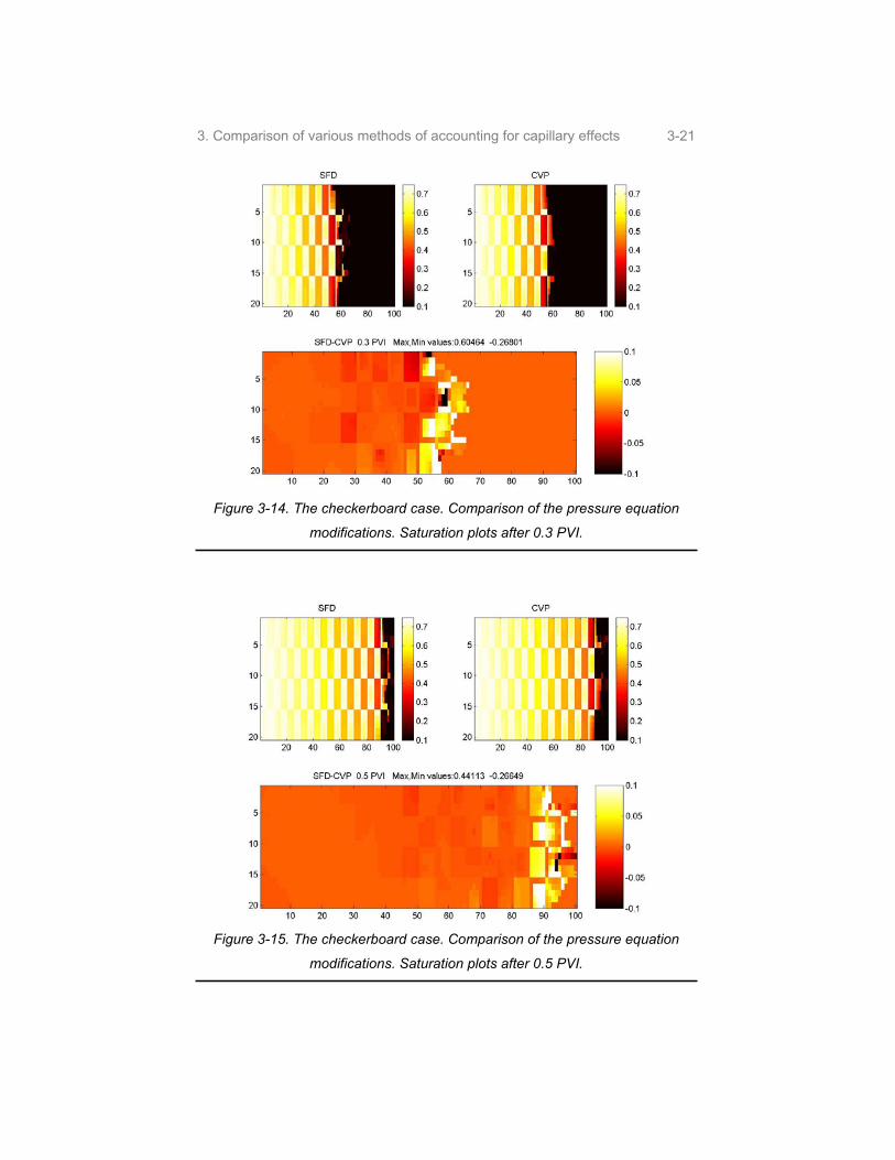
3. Comparison of various methods of accounting for capillary effects 3-21
Figure 3-14. The checkerboard case. Comparison of the pressure equation
modifications. Saturation plots after 0.3 PVI.
Figure 3-15. The checkerboard case. Comparison of the pressure equation
modifications. Saturation plots after 0.5 PVI.
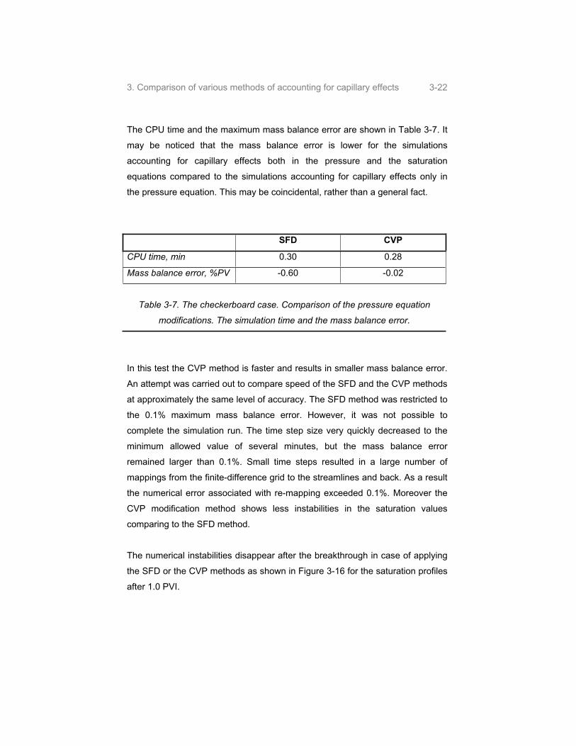
3. Comparison of various methods of accounting for capillary effects 3-22
The CPU time and the maximum mass balance error are shown in Table 3-7. It
may be noticed that the mass balance error is lower for the simulations
accounting for capillary effects both in the pressure and the saturation
equations compared to the simulations accounting for capillary effects only in
the pressure equation. This may be coincidental, rather than a general fact.
SFD CVP
CPU time, min 0.30 0.28
Mass balance error, %PV -0.60 -0.02
Table 3-7. The checkerboard case. Comparison of the pressure equation
modifications. The simulation time and the mass balance error.
In this test the CVP method is faster and results in smaller mass balance error.
An attempt was carried out to compare speed of the SFD and the CVP methods
at approximately the same level of accuracy. The SFD method was restricted to
the 0.1% maximum mass balance error. However, it was not possible to
complete the simulation run. The time step size very quickly decreased to the
minimum allowed value of several minutes, but the mass balance error
remained larger than 0.1%. Small time steps resulted in a large number of
mappings from the finite-difference grid to the streamlines and back. As a result
the numerical error associated with re-mapping exceeded 0.1%. Moreover the
CVP modification method shows less instabilities in the saturation values
comparing to the SFD method.
The numerical instabilities disappear after the breakthrough in case of applying
the SFD or the CVP methods as shown in Figure 3-16 for the saturation profiles
after 1.0 PVI.
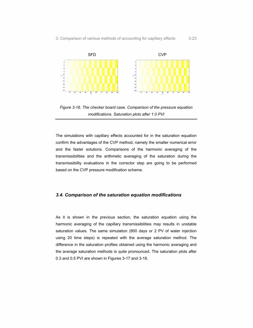
3. Comparison of various methods of accounting for capillary effects 3-23
SFD CVP
Figure 3-16. The checker board case. Comparison of the pressure equation
modifications. Saturation plots after 1.0 PVI
The simulations with capillary effects accounted for in the saturation equation
confirm the advantages of the CVP method, namely the smaller numerical error
and the faster solutions. Comparisons of the harmonic averaging of the
transmissibilities and the arithmetic averaging of the saturation during the
transmissibility evaluations in the corrector step are going to be performed
based on the CVP pressure modification scheme.
3.4. Comparison of the saturation equation modifications
As it is shown in the previous section, the saturation equation using the
harmonic averaging of the capillary transmissibilities may results in unstable
saturation values. The same simulation (800 days or 2 PV of water injection
using 20 time steps) is repeated with the average saturation method. The
difference in the saturation profiles obtained using the harmonic averaging and
the average saturation methods is quite pronounced. The saturation plots after
0.3 and 0.5 PVI are shown in Figures 3-17 and 3-18.

3. Comparison of various methods of accounting for capillary effects 3-24
Harmonic average Average saturation
Figure 3-17. The checkerboard case. Comparison of the saturation equation
modifications. Saturation plots after 0.3 PVI.
Harmonic average Average saturation
Figure 3-18. The checker board case. Comparison of the saturation equation
modifications. Saturation plots after 0.5 PVI.
Comparisons of the CPU times and the mass balance errors are presented in
Table 3-8.
Harmonic average Average saturation
CPU time, min 0.28 0.25
Mass balance error, %PV -0.02 -0.006
Table 3-8. The checkerboard case. Comparison of the saturation equation
modifications. The simulation time and the mass balance error.
The displacement profile looks more stable for the simulation using the average
saturation method. The results obtained using the average saturation are

3. Comparison of various methods of accounting for capillary effects 3-25
compared to the Eclipse 100. The Eclipse 100 simulations are performed in the
IMPES mode. The IMPES mode is selected to minimize the numerical
dispersion associated with the finite difference solution. The displacement
profiles after 0.3 and 0.5 PVI are compared to the Eclipse 100 are shown in
Figures 3-19 and 3-20. There are few pronounced differences between the
Eclipse and the CapSL for this simulation case. The Eclipse predicts stronger
end-effects between the high and the low permeable checker blocks and slower
propagation of water inside the low permeable checkers. The low permeable
checker blocks in the Eclipse simulation can be easily identified in Figures 3-19
and 3-20. The water saturation in the boundary layer of the preceding (in the
direction of the flow) high permeable checker-block is rather low. On the other
hand, the water saturation in the boundary low permeable grid blocks facing the
next high permeable checker-block is high. Both these effects are due to the
capillary end-effects, discussed later in this chapter.
Figure 3-19.The checkerboard case. Comparison of the Eclipse and the CapSL
saturation plots after 0.3 PVI.
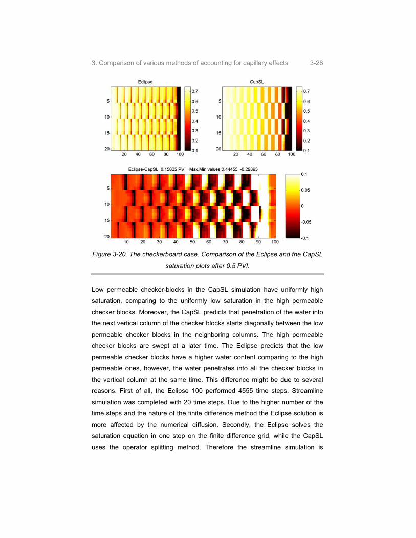
3. Comparison of various methods of accounting for capillary effects 3-26
Figure 3-20. The checkerboard case. Comparison of the Eclipse and the CapSL
saturation plots after 0.5 PVI.
Low permeable checker-blocks in the CapSL simulation have uniformly high
saturation, comparing to the uniformly low saturation in the high permeable
checker blocks. Moreover, the CapSL predicts that penetration of the water into
the next vertical column of the checker blocks starts diagonally between the low
permeable checker blocks in the neighboring columns. The high permeable
checker blocks are swept at a later time. The Eclipse predicts that the low
permeable checker blocks have a higher water content comparing to the high
permeable ones, however, the water penetrates into all the checker blocks in
the vertical column at the same time. This difference might be due to several
reasons. First of all, the Eclipse 100 performed 4555 time steps. Streamline
simulation was completed with 20 time steps. Due to the higher number of the
time steps and the nature of the finite difference method the Eclipse solution is
more affected by the numerical diffusion. Secondly, the Eclipse solves the
saturation equation in one step on the finite difference grid, while the CapSL
uses the operator splitting method. Therefore the streamline simulation is

3. Comparison of various methods of accounting for capillary effects 3-27
affected by the operator splitting error. Finally, the flow paths of the two
simulators are different. The flow path in the block-centered finite-difference
simulation is represented by the set of the straight lines connecting the block
centers. The streamline flow path is much more realistic, as sketched in Figure
3-21
Figure 3-21. The difference of the flow paths between finite-difference (solid
line) and streamline (dashed line) methods.
In general as a result of more realistic flow path and smaller numerical
dispersion the streamline simulation provide better prediction quality. However,
the operator splitting error may be rather large for the large time steps. The
comparison of the CapSL and the Eclipse results is performed using the
automatic time step selection routine, as shown in the next section.
3.5. Comparison of the time step selection routines
The stability condition for the finite-difference IMPES methods demands that the
saturation front does not propagate by more than one grid block per single time
step. Therefore, increasing the number of grid blocks by a factor of two requires
decreasing the time step size by a factor of two as well, leading to the second
order dependency of the simulation time from the grid size. For the streamline

3. Comparison of various methods of accounting for capillary effects 3-28
methods, however, the dependence is less straightforward, as discussed in
Section 2.2.7.
Comparison of the various time step routines is performed using the optimal
choice of the methods of accounting for capillary effects in the pressure and the
saturation equations – the CVP method and the average saturation method.
As it is was shown previously, the stable solution for the test case 1 with the
capillary effects is obtained using 20 time steps. However, the difference
between the Eclipse and the CapSL predictions is quite pronounced. The
CapSL predicts a faster front propagation, and a higher sweep of the low
permeable checker blocks, as shown in Figures 3-19 and 3-20.
The automatic time step routine presented in the Section 2.2.7, is applied. The
saturation profiles obtained using the automatic time step routine are compared
to the profiles obtained using 20 time steps in Figure 3-22. Comparison with the
Eclipse is shown in Figure 3-23. The comparisons of the CPU time and the
mass balance error are presented in Table 3-9.
20 time steps Automatic time steps
CPU time, sec 15 24 (138 time steps)
Mass balance error, %PV -0.006 -0.5
Table 3-9. The checkerboard case. Comparison of the time step routines. The
simulation time and the mass balance error.
The mass balance error for the simulation utilizing the automatic time step
routine is larger compared to the simulation using 20 time steps. Increase of the
mass balance error means that increase of the mapping error overcomes the
decrease of the operator splitting error.

3. Comparison of various methods of accounting for capillary effects 3-29
0.3PVI20 steps Automatic steps
0.5PVI20 steps Automatic steps
Figure 3-22. The checkerboard case. Comparison of the time step selection
routines.
Figure 3-23. The checkerboard case. Comparison of the Eclipse and the
CapSL(using automatic time steps) saturation plots after 0.5 PVI.
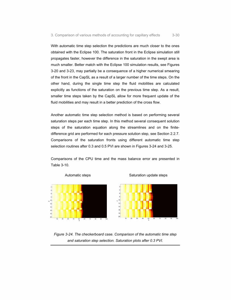
3. Comparison of various methods of accounting for capillary effects 3-30
With automatic time step selection the predictions are much closer to the ones
obtained with the Eclipse 100. The saturation front in the Eclipse simulation still
propagates faster, however the difference in the saturation in the swept area is
much smaller. Better match with the Eclipse 100 simulation results, see Figures
3-20 and 3-23, may partially be a consequence of a higher numerical smearing
of the front in the CapSL as a result of a larger number of the time steps. On the
other hand, during the single time step the fluid mobilities are calculated
explicitly as functions of the saturation on the previous time step. As a result,
smaller time steps taken by the CapSL allow for more frequent update of the
fluid mobilities and may result in a better prediction of the cross flow.
Another automatic time step selection method is based on performing several
saturation steps per each time step. In this method several consequent solution
steps of the saturation equation along the streamlines and on the finite-
difference grid are performed for each pressure solution step, see Section 2.2.7.
Comparisons of the saturation fronts using different automatic time step
selection routines after 0.3 and 0.5 PVI are shown in Figures 3-24 and 3-25.
Comparisons of the CPU time and the mass balance error are presented in
Table 3-10.
Automatic steps Saturation update steps
Figure 3-24. The checkerboard case. Comparison of the automatic time step
and saturation step selection. Saturation plots after 0.3 PVI.

3. Comparison of various methods of accounting for capillary effects 3-31
Automatic steps Saturation update steps
Figure 3-25. The checkerboard case. Comparison of the automatic time step
and saturation step selection. Saturation plots after 0.5 PVI.
Automatic time steps Automatic saturation
time steps
CPU time, min 0.41 (138 time steps) 1.1 (1010 saturation
steps)
Mass balance error, %PV -0.5 0.26
Table 3-10. The checkerboard case. Comparison of the time step and the
saturation step selection routines. The simulation time and the mass balance
error.
The automatic saturation step routine results in the slower run since it uses the
most restricted time step selection. It is possible that such a restriction is not
necessary for the streamline simulation, but the detailed research of the time
step selection routine is not included in this thesis.
The simulation using both automatic time step selection and automatic selection
of the saturation steps finished in 1.3 minutes, after 131 time steps and 1180
saturation steps, being the slowest streamline simulation run for the given test
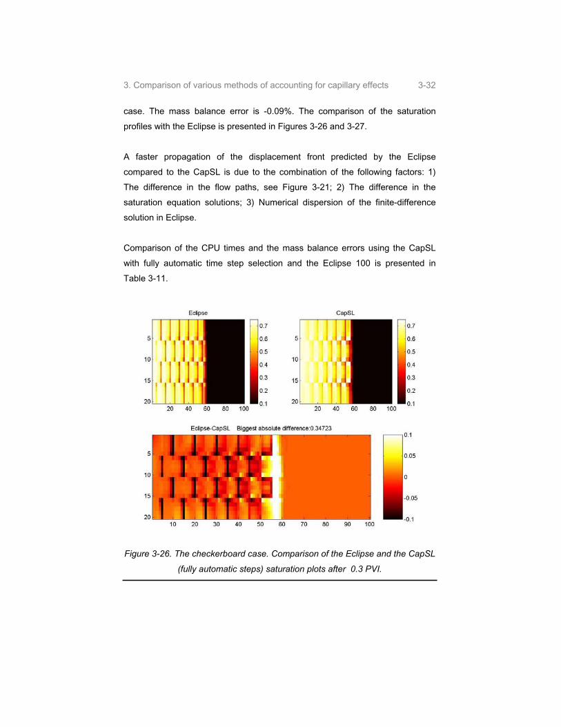
3. Comparison of various methods of accounting for capillary effects 3-32
case. The mass balance error is -0.09%. The comparison of the saturation
profiles with the Eclipse is presented in Figures 3-26 and 3-27.
A faster propagation of the displacement front predicted by the Eclipse
compared to the CapSL is due to the combination of the following factors: 1)
The difference in the flow paths, see Figure 3-21; 2) The difference in the
saturation equation solutions; 3) Numerical dispersion of the finite-difference
solution in Eclipse.
Comparison of the CPU times and the mass balance errors using the CapSL
with fully automatic time step selection and the Eclipse 100 is presented in
Table 3-11.
Figure 3-26. The checkerboard case. Comparison of the Eclipse and the CapSL
(fully automatic steps) saturation plots after 0.3 PVI.

3. Comparison of various methods of accounting for capillary effects 3-33
Figure 3-27. The checkerboard case. Comparison of the Eclipse and the CapSL
(fully automatic steps) saturation plots after 0.5 PVI.
Fully automatic steps Eclipse
CPU time, min 1.3 (1180 saturation
steps,131 time steps) 1.4 (4556 steps)
Mass balance error, %PV -0.09 0.06
Table 3-11. The checkerboard case. Comparison of the Eclipse and the
CapSL(fully automatic steps). The simulation time and the mass balance error.
Comparison of the oil production curves is presented in Figure 3-28. As a result
of faster propagation of the displacement front and lower local sweep efficiency
the Eclipse predicts faster breakthrough and slightly lower oil production.
However, the oil production curves have the same trend and are generally close
to each other.

3. Comparison of various methods of accounting for capillary effects 3-34
Pore Volumes of Water Injected
0.0 0.2 0.4 0.6 0.8 1.0 1.2 1.4 1.6 1.8 2.0
Por
e V
olum
es o
f Oil
Pro
duce
d
0.0
0.1
0.2
0.3
0.4
0.5
0.6
0.7
CapSLEclipse 100
Figure 3-28. The checkerboard case. Comparison of the Eclipse and the
CapSL(fully automatic steps). Oil production curves.
Based on the results presented above it may be concluded that the simulation
with fully automatic time step selection delivers the best match with the Eclipse
100 simulations. The mass balance error for the simulation with fully automatic
time step selection is comparable to the simulation using 20 time steps.
However, the CapSL simulation with automatic time step selection results in the
simulation times comparable to the Eclipse.
For the sake of the simulation speed one may use manual steps with restricted
maximum mass balance error. In case of the fluctuations in the saturation
values or a large number of rejected steps the automatic time step selection
routine may be applied.
3.6. Simulation of the two-dimensional heterogeneous case
First, the simulation of the test case 2 is performed neglecting capillary effects
to estimate the difference between the simulators in the numerical smearing of

3. Comparison of various methods of accounting for capillary effects 3-35
the saturation front. The saturation plots are compared in Figures 3-29 and 3-30
after 0.25 and 0.5 PVI.
Figure 3-29. Test case 2. Comparison of the Eclipse and the CapSL saturation
plots without capillary effects after 0.25 PVI.
Figure 3-30. Test case 2. Comparison of the Eclipse and the CapSL saturation
plots without capillary effects after 0.5 PVI.
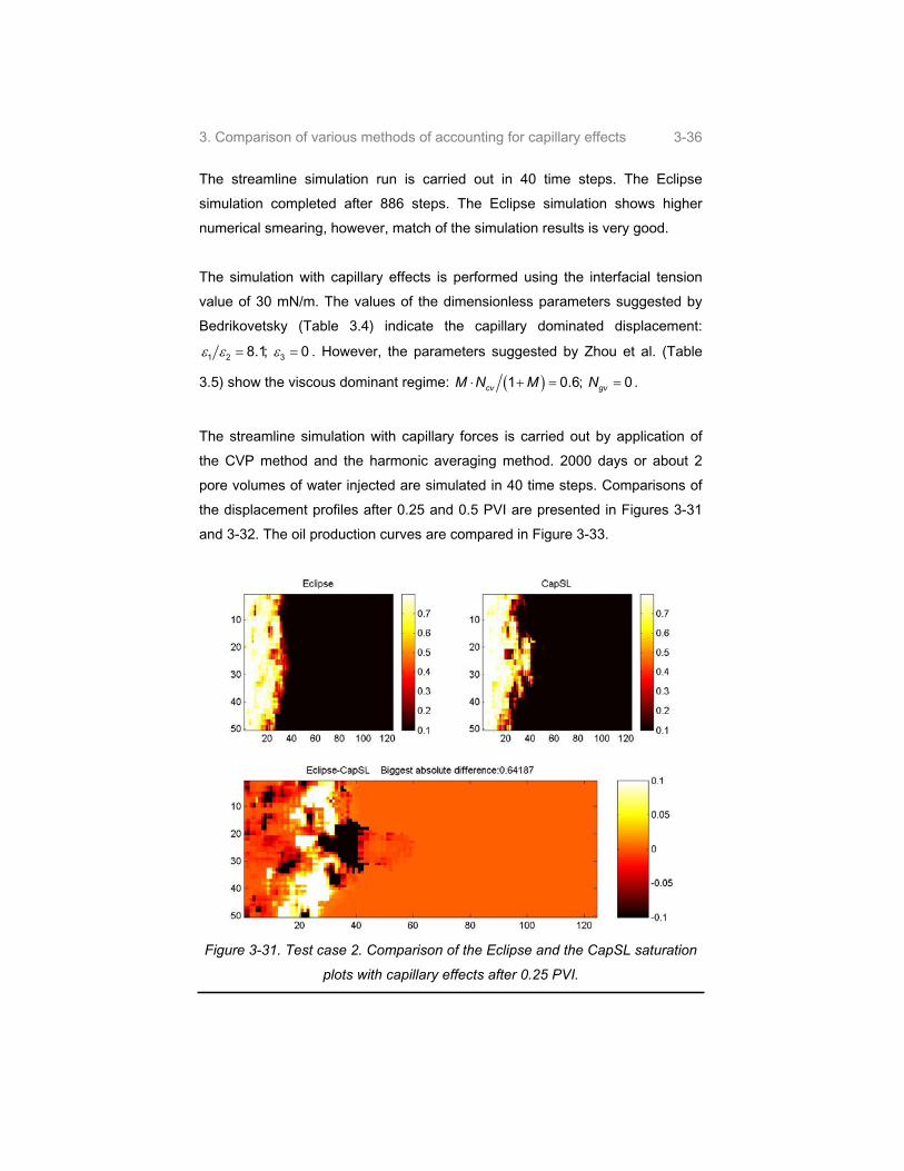
3. Comparison of various methods of accounting for capillary effects 3-36
The streamline simulation run is carried out in 40 time steps. The Eclipse
simulation completed after 886 steps. The Eclipse simulation shows higher
numerical smearing, however, match of the simulation results is very good.
The simulation with capillary effects is performed using the interfacial tension
value of 30 mN/m. The values of the dimensionless parameters suggested by
Bedrikovetsky (Table 3.4) indicate the capillary dominated displacement:
1 2 38.1; 0 . However, the parameters suggested by Zhou et al. (Table
3.5) show the viscous dominant regime: 1 0.6; 0cv gvM N M N .
The streamline simulation with capillary forces is carried out by application of
the CVP method and the harmonic averaging method. 2000 days or about 2
pore volumes of water injected are simulated in 40 time steps. Comparisons of
the displacement profiles after 0.25 and 0.5 PVI are presented in Figures 3-31
and 3-32. The oil production curves are compared in Figure 3-33.
Figure 3-31. Test case 2. Comparison of the Eclipse and the CapSL saturation
plots with capillary effects after 0.25 PVI.

3. Comparison of various methods of accounting for capillary effects 3-37
Figure 3-32. Test case 2. Comparison of the Eclipse and the CapSL saturation
plots with capillary effects after 0.5 PVI.
Pore Volumes of Water Injected
0.0 0.2 0.4 0.6 0.8 1.0 1.2 1.4 1.6 1.8 2.0
Por
e V
olum
es o
f Oil
Pro
duce
d
0.0
0.2
0.4
0.6
0.8
CapSLEclipse 100CapSL, IFT=30 mN/mEclipse, IFT=30 mN/m
Figure 3-33. Test case 2. Comparison of the Eclipse and the CapSL oil
production curves.

3. Comparison of various methods of accounting for capillary effects 3-38
The difference between the saturation profiles for the simulations including and
neglecting capillary effects is rather large; however the difference in the oil
production curves is quite modest.
The simulators performance data is gathered in Table 3-12.
Neglecting cap. eff. With cap. eff.
CapSL Eclipse CapSL Eclipse
CPU time, min 0.34 (40
time steps)
2 (886
steps)
2.93 (40
time steps)
8 (6981
steps)
Mass bal. error, %PV 0.14 ~0 0.04 ~0
Table 3-12. Test case 2. Comparison of the Eclipse and the CapSL. The
simulation time and the mass balance error.
The CapSL is around 3 times faster comparing to the IMPES Eclipse 100
simulations. The mass balance error is higher for the simulations performed
with the CapSL, however, it remains below 0.2%. Judging by Table 3-12, the
Eclipse code is much better optimized comparing to the CapSL. For the
simulation with capillary effects a single time step in the Eclipse takes around
0.07 seconds. A single time step in the CapSL is around 1.8 seconds. The
function timing profile of the CapSL simulation shows that the most time
consuming routines are: 1) The corrector step, consuming around 1/3 of the
simulation time; 2) The routine calculating the linear approximation of the
tabulated values consuming around 1/3 of the simulation time. According to the
profile, a single call of this routine lasts only about 1 10-4 millisecond. However,
this routine is used for calculating all the physical properties of the phases as
functions of saturation, including the relative permeabilities, fractional flow
function, and the Leverett function, and it is called around 300 million times in
the current simulation run. For the simulation without capillary effects the
corrector routine is not used, and the number of calls to the linear approximation
routine is significantly smaller as well, resulting in lower simulation time, as
shown in Table 3-12.

3. Comparison of various methods of accounting for capillary effects 3-39
The streamline simulator shows a higher oil production for the simulations both
neglecting and accounting for capillary effects. For the simulation neglecting the
capillary effects the higher oil production is due to the later breakthrough as a
result of the smaller dispersion of the front. The slopes of the oil production
curves after the breakthrough predicted by the CapSL and the Eclipse are in a
good agreement. For the simulation with capillary effects both simulators agree
on the breakthrough time, however, due to higher local sweep efficiency the
CapSL predicts higher oil production again.
The displacement front predicted by the Eclipse shows slower sweeping of the
high permeable blocks, see Figures 3-29 and 3-30. Some of these zones
remain less swept, comparing to the CapSL even after two pore volumes of
water injected, as shown in Figure 3-34.
Figure 3-34. Test case 2. Comparison of the Eclipse and the CapSL saturation
plots with capillary effects after 2PVI.

3. Comparison of various methods of accounting for capillary effects 3-40
The high permeable blocks are swept as soon as the water saturation in the
surrounding blocks rises to the maximum value. The only explanation of slower
sweep of the high permeable blocks predicted by Eclipse is that due to the
numerical dispersion the saturation increases very slowly to the maximum water
saturation, allowing water to flow around the high permeable zone. The low
permeable blocks surrounding the high permeable block in the row 9, column
10 in Figure 3-34 (shown with the green arrow) have a water saturation of 0.80
after 2.0 PVI, as predicted by CapSL. The Eclipse shows the water saturation
value of around 0.77 – 0.79.
The mass balance error and the CPU time of two different pressure modification
methods are shown in Table 3-13.
CVP + harmonic
averaging
SFD + harmonic
averaging
CPU time, min 2.93 2.2
Mass. bal. error, %PV 0.04 -0.26
Table 3-13. Test case 2. Comparison of the CVP and the SFD modifications.
The simulation time and the mass balance error.
The SFD method shows no difference in the displacement behavior comparing
to the CVP method.
The results presented in Table 3-13 show that for the large scale stochastically
heterogeneous simulations with strong capillary forces it is not necessary to use
the automatic time step selection routine. Moreover, the simulation with
automatic time step selection routine uses 943 steps, and takes nearly two
hours. The simulation results in a large mass balance error due to the mapping
error.
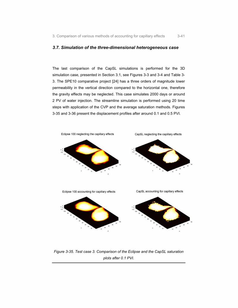
3. Comparison of various methods of accounting for capillary effects 3-41
3.7. Simulation of the three-dimensional heterogeneous case
The last comparison of the CapSL simulations is performed for the 3D
simulation case, presented in Section 3.1, see Figures 3-3 and 3-4 and Table 3-
3. The SPE10 comparative project [24] has a three orders of magnitude lower
permeability in the vertical direction compared to the horizontal one, therefore
the gravity effects may be neglected. This case simulates 2000 days or around
2 PV of water injection. The streamline simulation is performed using 20 time
steps with application of the CVP and the average saturation methods. Figures
3-35 and 3-36 present the displacement profiles after around 0.1 and 0.5 PVI.
Figure 3-35. Test case 3. Comparison of the Eclipse and the CapSL saturation
plots after 0.1 PVI.
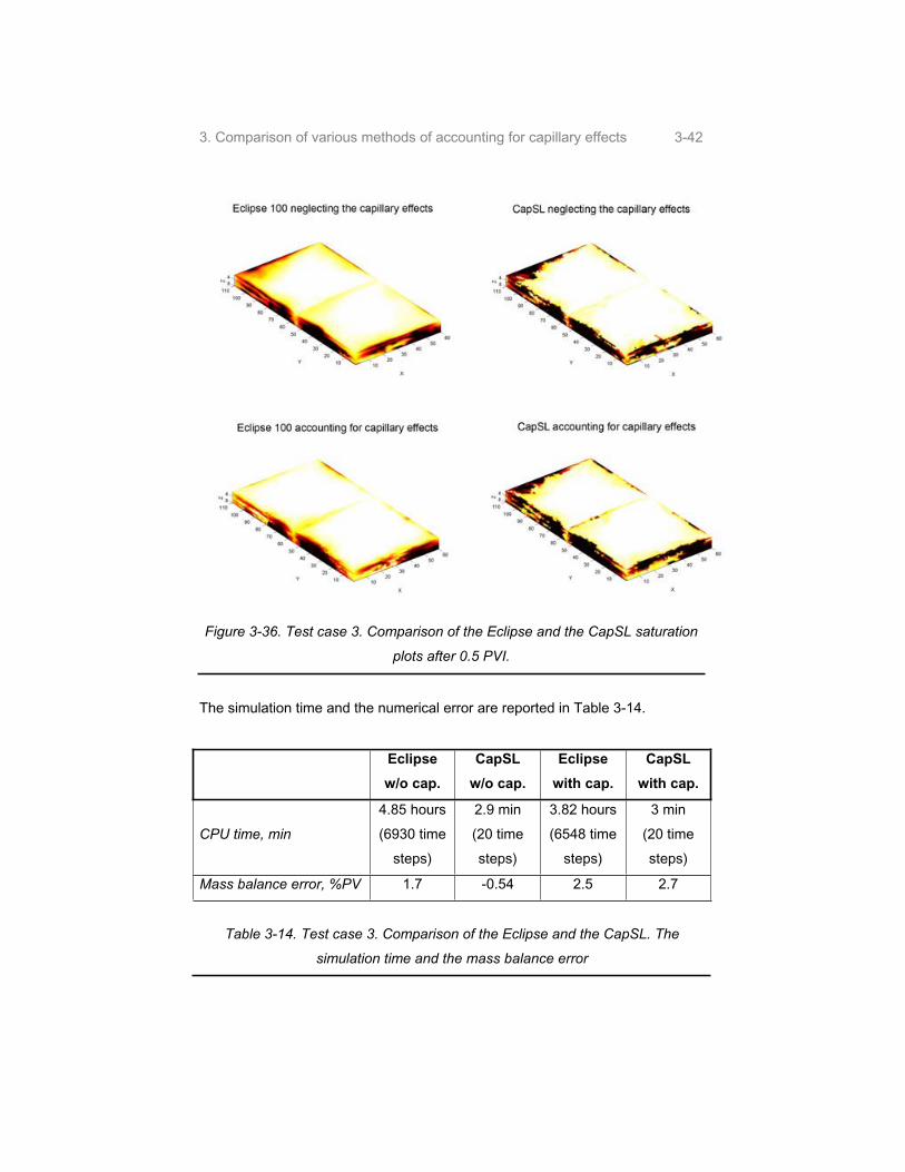
3. Comparison of various methods of accounting for capillary effects 3-42
Figure 3-36. Test case 3. Comparison of the Eclipse and the CapSL saturation
plots after 0.5 PVI.
The simulation time and the numerical error are reported in Table 3-14.
Eclipse
w/o cap.
CapSL
w/o cap.
Eclipse
with cap.
CapSL
with cap.
CPU time, min
4.85 hours
(6930 time
steps)
2.9 min
(20 time
steps)
3.82 hours
(6548 time
steps)
3 min
(20 time
steps)
Mass balance error, %PV 1.7 -0.54 2.5 2.7
Table 3-14. Test case 3. Comparison of the Eclipse and the CapSL. The
simulation time and the mass balance error
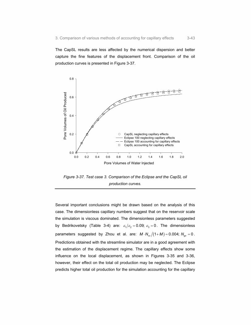
3. Comparison of various methods of accounting for capillary effects 3-43
The CapSL results are less affected by the numerical dispersion and better
capture the fine features of the displacement front. Comparison of the oil
production curves is presented in Figure 3-37.
Pore Volumes of Water Injected
0.0 0.2 0.4 0.6 0.8 1.0 1.2 1.4 1.6 1.8 2.0
Por
e V
olum
es o
f Oil
Pro
duce
d
0.0
0.2
0.4
0.6
0.8
CapSL neglecting capillary effectsEclipse 100 neglecting capillary effectsEclipse 100 accounting for capillary effectsCapSL accounting for capillary effects
Figure 3-37. Test case 3. Comparison of the Eclipse and the CapSL oil
production curves.
Several important conclusions might be drawn based on the analysis of this
case. The dimensionless capillary numbers suggest that on the reservoir scale
the simulation is viscous dominated. The dimensionless parameters suggested
by Bedrikovetsky (Table 3-4) are: 1 2 30.09; 0 . The dimensionless
parameters suggested by Zhou et al. are: 1 0.004; 0cv gvM N M N .
Predictions obtained with the streamline simulator are in a good agreement with
the estimation of the displacement regime. The capillary effects show some
influence on the local displacement, as shown in Figures 3-35 and 3-36,
however, their effect on the total oil production may be neglected. The Eclipse
predicts higher total oil production for the simulation accounting for the capillary
3. Comparison of various methods of accounting for capillary effects 3-44
effects, compared to the one neglecting the capillary effects. Such behavior
might be explained by comparable orders of magnitude of the capillary forces
and the numerical dispersion in the Eclipse simulations. Hence, the
breakthrough predicted by the Eclipse without capillary forces happens sooner,
compared to the CapSL, resulting in a lower total oil production. The oil
production curves predicted by the CapSL and the Eclipse for the simulation
with capillary effects show a good agreement.
The SFD and the CVP methods show excellent match as well. Both the CVP
and the SFD simulations complete in about 3 minutes and have the same mass
balance error. Simulations with average saturation do not improve the CapSL
performance as well.
Both the Eclipse and the CapSL simulations result in rather high volume
balance errors. The CapSL simulations with automatic time step selection
routines resulted in the same volume balance error.
3.8. Comparison summary
Based on the simulation cases presented in this chapter, the two simulation
types may be distinguished.
The first type is the simulations of the heterogeneous reservoirs comprised of
two and more homogeneous zones with several well-defined permeability
borders. Typically, such kinds of runs are used for the simulation of the
laboratory scale displacements or the preliminary assessment of the models on
the simple permeability data. The CVP method may be recommended to speed
up the simulation and to decrease the numerical error. The average saturation
method should be chosen to provide correct description of the capillary cross
flow through the permeability borders. The application of the automatic time
3. Comparison of various methods of accounting for capillary effects 3-45
step routines facilitates better mach with the Eclipse simulation results, but may
also result in larger numerical errors.
For the simulations of the stochastically heterogeneous or similar reservoirs
with varying permeability and / or porosity it is advisable to take large time
steps. The time steps may be restricted by specifying the maximum mass
balance error. There is no principal difference in the simulations using various
methods of accounting for capillary effects in the pressure and the saturation
equations. Typically, such runs represent the full-scale simulation of the
reservoir data. The streamline simulator may be used as a tool to access the
difficulties and visualize the relative strength of the capillary and the
gravitational forces as well as the main reservoir simulation tool.


4-1
4. Sample calculations and effects
This chapter starts with illustration and discussion of the capillary end-effects.
The effect of the rock wettability on the capillary forces is discussed. Streamline
simulations of alternated wet media are presented.
Later in the chapter the CapSL is tested in the range of capillary forces and
mobility ratios corresponding to water / oil displacements.
The chapter concludes with the CapSL and the Eclipse 100 [62] simulations of
the lab-scale data kindly provided by Yildiray Cinar, SUPRI-C, Department of
Petroleum Engineering, Stanford University.
4.1 Capillary effects in porous media
Capillary effects in porous media may be separated into the three groups:
Smearing of the saturation front by capillary effects;
Capillary effects on the borders of the media with different permeability;
Capillary effects on the borders of the media with different wettability.
This section is divided into the two parts. First, the water wet media is
investigated, the effects of heterogeneity in the water wet reservoirs are
presented. Later, the alternated wet media is simulated.
4.1.1. Capillary effects in water wet medium
The front smearing effects are illustrated on a simple one-dimensional
laboratory-scale 1D case. The simulation grid is comprised of 1500 grid blocks.
The sample is 15 5 5 cm in size. The production pressure is 1 atm; the injection

4. Sample calculations and effects 4-2
rate is 6.25 cc/h. The relative permeability curves and the J-function are taken
from the test case 3, see Table 3-3. The initial water saturation is 0.1. The water
viscosity is 0.7cP, the oil viscosity is 0.9cP. The interfacial tension between the
fluids is set to 0.3 mN/m. The sample permeability is 400mD. 4 hours of water
injection are simulated. The simulation is capillary dominated
with 1 24.5, 0.11.
The displacement profiles after 3, 5 and 10 time steps obtained with the CapSL
are presented in Figure 4-1.
Smearing of the saturation front is due to the gradient of the Leverett function
and happens in heterogeneous and homogeneous, water wet and oil wet
porous media [13]. For the one-dimensional case the simulation neglecting
capillary effects is described by the Buckley-Leverett equation [22]. The one-
dimensional simulation accounting for capillary effects is described by the
Rappoport – Leas equation [58].
Block number
0 10 20 30 40 50 60 70 80 90 100 110 120 130 140 150
Wat
er s
atur
atio
n
0.0
0.2
0.4
0.6
0.8
1.0Buckley - Leverett profile after time step 3Buckley - Leverett profile after time step 5Buckley - Leverett profile after time step 10Rapoport - Leas profile after step 3Rapoport - Leas profile after step 5Rapoport - Leas profile after step 10
Figure 4-1. 1D saturation profiles neglecting and accounting for capillary effects.
The capillary cross-flow is illustrated by simulating a part of the reservoir. The
sample is 150 1 1 m and simulated on the 1D grid with 1500 grid blocks. The
fluid data is taken from the test case 3, see Table 3-3. The capillary to viscous
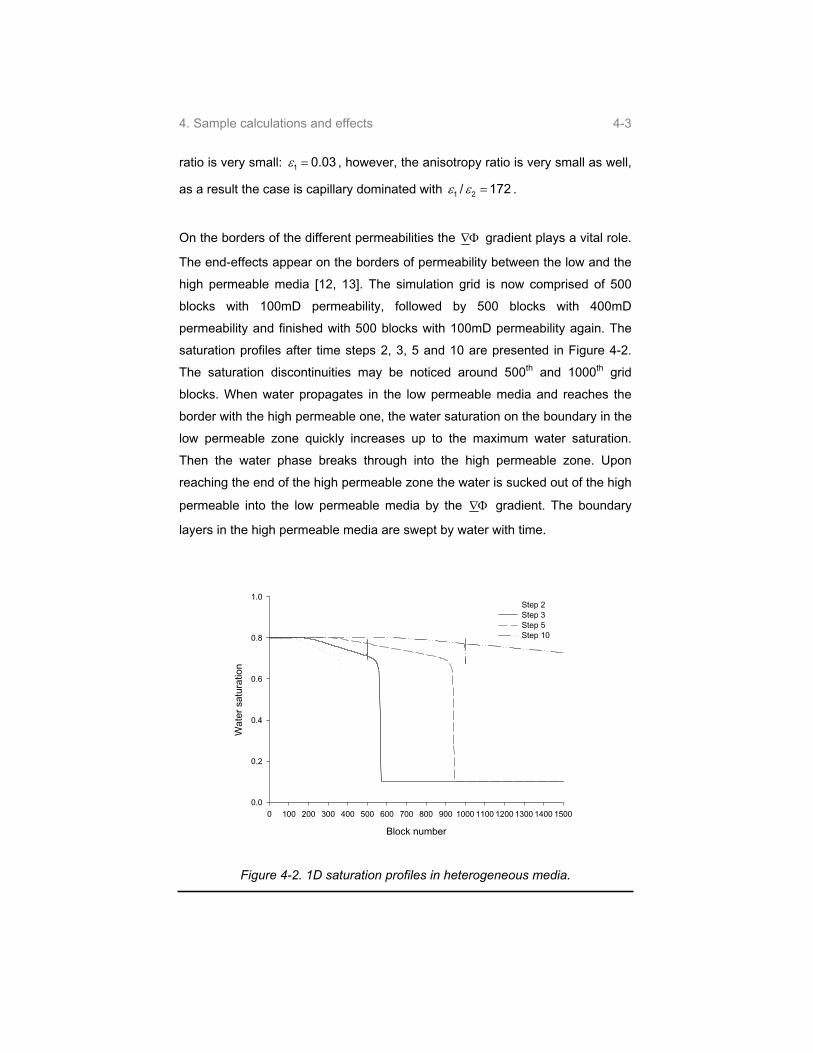
4. Sample calculations and effects 4-3
ratio is very small: 1 0.03 , however, the anisotropy ratio is very small as well,
as a result the case is capillary dominated with 1 2/ 172 .
On the borders of the different permeabilities the gradient plays a vital role.
The end-effects appear on the borders of permeability between the low and the
high permeable media [12, 13]. The simulation grid is now comprised of 500
blocks with 100mD permeability, followed by 500 blocks with 400mD
permeability and finished with 500 blocks with 100mD permeability again. The
saturation profiles after time steps 2, 3, 5 and 10 are presented in Figure 4-2.
The saturation discontinuities may be noticed around 500th and 1000th grid
blocks. When water propagates in the low permeable media and reaches the
border with the high permeable one, the water saturation on the boundary in the
low permeable zone quickly increases up to the maximum water saturation.
Then the water phase breaks through into the high permeable zone. Upon
reaching the end of the high permeable zone the water is sucked out of the high
permeable into the low permeable media by the gradient. The boundary
layers in the high permeable media are swept by water with time.
Block number
0 100 200 300 400 500 600 700 800 900 1000 1100 1200 1300 1400 1500
Wat
er s
atur
atio
n
0.0
0.2
0.4
0.6
0.8
1.0Step 2 Step 3 Step 5 Step 10
Figure 4-2. 1D saturation profiles in heterogeneous media.

4. Sample calculations and effects 4-4
The simulations demonstrated above are one-dimensional and homogeneous in
the transverse direction. In order to investigate the cross flow effect, the two
dimensional simulation system is used as sketched in Figure 4-3.
The top layer is homogeneous and consists of low permeable Rock1 with the
permeability of 100mD. The bottom layer consists of Rock1 and Rock2 with the
permeability of 400mD. Both Rock1 and Rock2 are water wet. The size of the
grid blocks is 1 1 1m as in the 1D simulation. The pore volume of the 2D
simulation sketched in Figure 4-3 is twice as large as the pore volume of the 1D
simulations presented at the beginning of this section. To be able to compare
the results to the 1D simulation the injection rate is doubled. The results are
shown in Figure 4-4.
Rock1
Rock1 Rock2 Rock1
50 blocks50 blocks50 blocks
2blocks
Homogeneous layer
Heterogeneous layer
Figure 4-3. 2D cross flow investigation grid.
The saturation profiles in the heterogeneous layer are compared to the 1D
profiles in Figure 4-2. The homogeneous layer saturation profiles are compared
to the homogeneous 1D profiles from Figure 4-1.
As it may be seen from Figure 4-4, the saturation profiles in the first 500 blocks
of the 2D simulation match with corresponding 1D profiles.
Differences in the saturation profiles in both homogeneous and heterogeneous
layers appear in the Rock2 zone, above it and right after it. The saturation in the
Rock2 zone is lower compared to the 1D simulation due to the capillary cross
flow. The water is transferred into more preferable Rock1 above, therefore the
water saturation in the homogeneous layers is higher comparing to the 1D
profile.
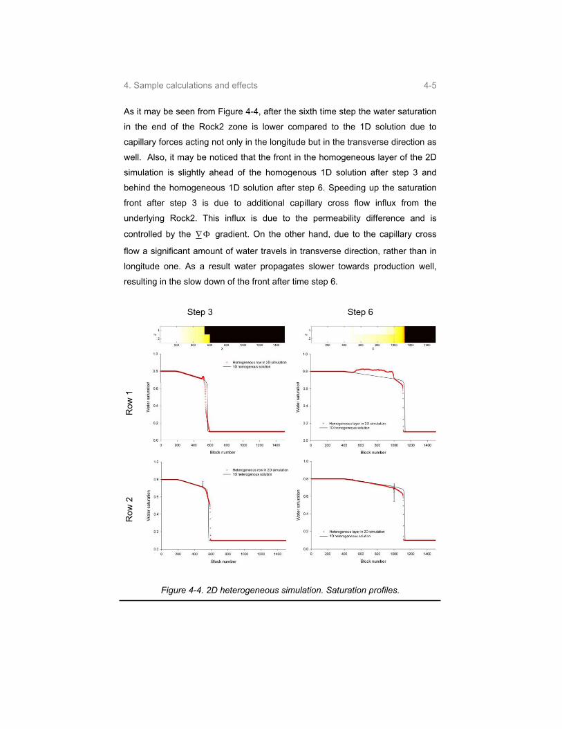
4. Sample calculations and effects 4-5
As it may be seen from Figure 4-4, after the sixth time step the water saturation
in the end of the Rock2 zone is lower compared to the 1D solution due to
capillary forces acting not only in the longitude but in the transverse direction as
well. Also, it may be noticed that the front in the homogeneous layer of the 2D
simulation is slightly ahead of the homogenous 1D solution after step 3 and
behind the homogeneous 1D solution after step 6. Speeding up the saturation
front after step 3 is due to additional capillary cross flow influx from the
underlying Rock2. This influx is due to the permeability difference and is
controlled by the gradient. On the other hand, due to the capillary cross
flow a significant amount of water travels in transverse direction, rather than in
longitude one. As a result water propagates slower towards production well,
resulting in the slow down of the front after time step 6.
Step 3 Step 6
Figure 4-4. 2D heterogeneous simulation. Saturation profiles.
Row
2
Row
1
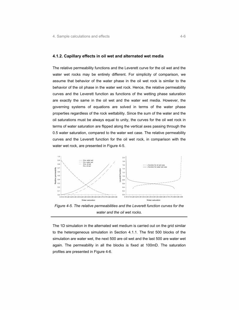
4. Sample calculations and effects 4-6
4.1.2. Capillary effects in oil wet and alternated wet media
The relative permeability functions and the Leverett curve for the oil wet and the
water wet rocks may be entirely different. For simplicity of comparison, we
assume that behavior of the water phase in the oil wet rock is similar to the
behavior of the oil phase in the water wet rock. Hence, the relative permeability
curves and the Leverett function as functions of the wetting phase saturation
are exactly the same in the oil wet and the water wet media. However, the
governing systems of equations are solved in terms of the water phase
properties regardless of the rock wettability. Since the sum of the water and the
oil saturations must be always equal to unity, the curves for the oil wet rock in
terms of water saturation are flipped along the vertical axes passing through the
0.5 water saturation, compared to the water wet case. The relative permeability
curves and the Leverett function for the oil wet rock, in comparison with the
water wet rock, are presented in Figure 4-5.
Water saturation
0.10 0.15 0.20 0.25 0.30 0.35 0.40 0.45 0.50 0.55 0.60 0.65 0.70 0.75 0.80 0.85 0.90
Rea
ltive
per
mea
bilit
y
0.0
0.1
0.2
0.3
0.4
0.5
0.6
0.7
0.8
0.9
1.0
Krw, water wetKro, water wetKrw, oil wetKro, oil wet
Water saturation
0.10 0.15 0.20 0.25 0.30 0.35 0.40 0.45 0.50 0.55 0.60 0.65 0.70 0.75 0.80 0.85 0.90
Leve
rett
func
tion
0.0
0.2
0.4
0.6
0.8
1.0
1.2
1.4
1.6
1.8
2.0
J-function for oil wet caseJ-function for water wet case
Figure 4-5. The relative permeabilities and the Leverett function curves for the
water and the oil wet rocks.
The 1D simulation in the alternated wet medium is carried out on the grid similar
to the heterogeneous simulation in Section 4.1.1. The first 500 blocks of the
simulation are water wet, the next 500 are oil wet and the last 500 are water wet
again. The permeability in all the blocks is fixed at 100mD. The saturation
profiles are presented in Figure 4-6.

4. Sample calculations and effects 4-7
In general, the behavior of the saturation profiles in the water wet regions is
similar to the heterogeneous water wet simulation, Figure 4-2.
The water saturation in the oil wet zone does not show a drop as in the
heterogeneous water wet simulation. The main reason for this lies in the
difference in the relative permeabilities and the Leverett function curves in the
oil wet zone compared to the water wet one.
The saturation region where the water phase is mobile is also different. Water in
the water wet media is mobile if its saturation is above 0.1. The oil in the water
wet media is mobile if its saturation is above 0.2. In the oil wet media the water
saturation has to be above 0.2 and the oil saturation above 0.1 for the phases to
be mobile. This leads to higher water saturation in the oil wet zone, compared to
the water wet one.
Block number
0 100 200 300 400 500 600 700 800 900 1000 1100 1200 1300 1400 1500
Wat
er s
atur
atio
n
0.0
0.2
0.4
0.6
0.8
1.0Step 2 Step 3 Step 5 Step 10
Figure 4-6. 1D saturation profiles for alternated wet reservoir.
The 2D alternated wet simulation is performed on the grid presented in Figure
4-3.
The permeabilities of Rock1 and the Rock2 are fixed at 100mD. The Rock1 is
water wet, the Rock2 is oil wet. The saturation profiles are shown in Figure 4-7.

4. Sample calculations and effects 4-8
The capillary forces between the oil wet and the water wet media are much
stronger, compared to the capillary forces between the zones with different
permeabilities. The maximum capillary pressure difference in the water wet
media may be achieved on a border of the zones with different heterogeneities:
,max max mincP high perm J s low perm J s . (4.1)
The maximum capillary pressure difference for the homogeneous alternated wet
case is:
,max max minc water wet oil wetP J s J s . (4.2)
The positive sign in equation (4.2) is due to cos 1 in the oil wet media.
Stronger capillary forces between Rock2 and Rock1 result in the saturation
"hump" inside the Rock2 zone, see Step 6 in Figure 4-7.
Step 3 Step 6
Figure 4-7. Alternated-wetting medium simulation. Saturation profiles.
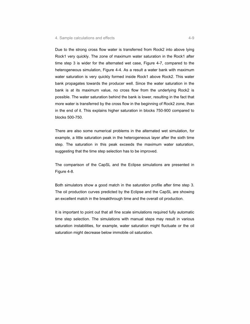
4. Sample calculations and effects 4-9
Due to the strong cross flow water is transferred from Rock2 into above lying
Rock1 very quickly. The zone of maximum water saturation in the Rock1 after
time step 3 is wider for the alternated wet case, Figure 4-7, compared to the
heterogeneous simulation, Figure 4-4. As a result a water bank with maximum
water saturation is very quickly formed inside Rock1 above Rock2. This water
bank propagates towards the producer well. Since the water saturation in the
bank is at its maximum value, no cross flow from the underlying Rock2 is
possible. The water saturation behind the bank is lower, resulting in the fact that
more water is transferred by the cross flow in the beginning of Rock2 zone, than
in the end of it. This explains higher saturation in blocks 750-900 compared to
blocks 500-750.
There are also some numerical problems in the alternated wet simulation, for
example, a little saturation peak in the heterogeneous layer after the sixth time
step. The saturation in this peak exceeds the maximum water saturation,
suggesting that the time step selection has to be improved.
The comparison of the CapSL and the Eclipse simulations are presented in
Figure 4-8.
Both simulators show a good match in the saturation profile after time step 3.
The oil production curves predicted by the Eclipse and the CapSL are showing
an excellent match in the breakthrough time and the overall oil production.
It is important to point out that all fine scale simulations required fully automatic
time step selection. The simulations with manual steps may result in various
saturation instabilities, for example, water saturation might fluctuate or the oil
saturation might decrease below immobile oil saturation.

4. Sample calculations and effects 4-10
Figure 4-8. Comparison of the CapSL and the Eclipse simulations for alternated
wet reservoir.
4.2. Zone of application of the streamline simulator with
capillary effects
In Section 3.1 it is shown that the simulation grids comprised of the
homogeneous zones are more complicated to handle using the streamline
simulator comparing to the stochastically heterogeneous media. Therefore the
two-dimensional system, comprised of two zones with different permeability is
selected for determination of the zone of application, as sketched in Figure 4-9.
The run data are collected in Table 4-1. The values of phase viscosities and
interfacial tension vary between the runs and are reported in Table 4-2. The
phase densities are set to equal values to completely remove gravity effects.
4. Sample calculations and effects 4-11
This case represents a simplified stratified reservoir, in which the capillary
effects play a vital role in distribution of the fluids between the zones of different
permeabilities. This case is simple enough, so that the effects of capillary forces
and phase mobility variations may easily be interpreted.
5
10
15
20 20 40 60 80 100 120 140 160 180 200
X
y
Figure 4-9. The permeability field for investigation the zone of application of the
streamline simulator with capillary effects.
The low permeable zone has the permeability of 50mD and is shown in black
color in Figure 4-9. The high permeable zone has the permeability of 400mD
and is shown in white in Figure 4-9.
The streamline simulations are performed applying the CVP method and the
average saturation method in the saturation equation. The automatic time step
selection routine is applied as well.
The Eclipse 100 simulations are performed in the IMPES mode. The
simulations are performed on the 200 20 grid. The convergence of the
numerical schemes is checked by refining the grid to 400 40. The difference in
the oil production curves on the different grids is below 0.5% relative to the pore
volumes of water injected.

4. Sample calculations and effects 4-12
Parameter Value
Simulation grid 200 20 areal slice; 4 4 1 m grid blocks
Porosity 0.4
Pore volume 25600 m3
Densities Water – 1000 kg/m3 Oil – 1000 kg/m3
Relative
permeabilities
2
2
1
11
0.8
0.9
0.1
0.25
wirw rwor
wi or
wiro rowi
wi or
rwor
rowi
wi
or
s sk k
s s
s sk k
s s
k
k
s
sWater saturation
0.10 0.15 0.20 0.25 0.30 0.35 0.40 0.45 0.50 0.55 0.60 0.65 0.70 0.75
Rea
ltive
per
mea
bilit
y
0.0
0.1
0.2
0.3
0.4
0.5
0.6
0.7
0.8
0.9
1.0
Relative permeability to waterRelative permeability to oil
Injection rate 2.0 m3/day (1 pore volume injected in 12800 days)
Production
pressure
20.0 MPa (producer located on the right)
111
( ) 1 , 1 1
nm
min
max min
s sJ s y n
s s m
Capillary
pressure
0.5
0.93
0.05
0.0999min
m
y
s
0.25maxs
Water saturation
0.1 0.2 0.3 0.4 0.5 0.6 0.7
Leve
rett
func
tion
0.0
0.2
0.4
0.6
0.8
1.0
1.2
Table 4-1. The simulation data for investigation the zone of application of the
streamline simulator with capillary effects.

4. Sample calculations and effects 4-13
Run number IFT ( )
mN/m
o
cP
w
cP1 2 M
Displ.
regime
1 0 1 1 0.058 0.89 Viscous
2 1 1 1 0.292 0.89 Viscous
3 10 1 1 2.916 0.89 Capillary
4 30 1 1 8.748 0.89 Capillary
5 0 5 1 0.000 4.49 Viscous
6 0 10 1 0.000 8.89 Viscous
7 0 20 1 0.000 17.78 Viscous
8 1 5 1 0.058 4.44 Viscous
9 10 5 1 0.583 4.44 Viscous
10 30 5 1 1.750 4.44 Capillary
11 1 10 1 0.029 8.89 Viscous
12 30 10 1 0.875 8.89 Viscous
13 1 20 1 0.015 17.78 Viscous
14 30 20 1 0.437 17.78 Viscous
15 72 20 1 1.048 17.78 Viscous
Table 4-2. Run specific data for investigation the zone of application of the
streamline simulator with capillary effects.
The parameters presented in Table 4-2 cover a wide range of mobility ratios
and interfacial tensions typical for reservoir simulation problems. The results are
divided into three groups: 1) Varying interfacial tension at constant mobility ratio
; 2) Varying mobility ratio at constant interfacial tension; 3) Varying both
interfacial tension and mobility ratio.The simulation times for the various runs
are not compared since all the runs took less than a minute. However, the
number of time steps and the mass balance error are reported for each run in
Table 4-3.

4. Sample calculations and effects 4-14
Eclipse CapSLRun number
IFT
mN/mM
steps error, % PV steps error, %PV
1 0 0.89 1276 -1.1*10-5 149 0.39
2 1 0.89 1376 1.50*10-5 156 0.33
3 10 0.89 1307 -2.90*10-7 204 0.26
4 30 0.89 1252 -1.70*10-4 235 0.31
5 0 4.49 778 -2.50*10-7 47 0.39
6 0 8.89 707 8.08*10-7 50 0.51
7 0 17.78 668 -1.20*10-6 56 0.58
8 1 4.44 891 -6.10*10-7 62 0.30
9 10 4.44 920 1.26*10-6 108 0.13
10 30 4.44 905 -1.40*10-4 136 0.21
11 1 8.89 788 3.22*10-6 60 0.42
12 30 8.89 840 -6.20*10-5 129 0.26
13 1 17.78 735 1.09*10-6 62 0.45
14 30 17.78 819 3.25*10-6 138 0.25
15 72 17.78 848 -1.10*10-4 197 0.07
Table 4-3. Investigation of the zone of application of the streamline simulator with
capillary effects. Number of time steps and simulation errors.
The mass balance error in all the Eclipse 100 simulations is fairly close to zero.
The error in the CapSL simulations is higher; however, it does not exceed the
value of 0.51 %PV. The streamline simulator performs 4 to 16 times less time
steps. The dependency of the number of time steps as a function of the mobility
ratio is presented in Figure 4-10. The dependency of the number of time steps
as a function of interfacial tension is presented in Figure 4-11.

4. Sample calculations and effects 4-15
Mobility ratio
0 2 4 6 8 10 12 14 16 18 20
Num
ber
step
s
0
200
400
600
800
1000
1200
1400
1600
EclipseCapSL
Figure 4-10. Investigation of the zone of application of the streamline simulator
with capillary effects. Number of time steps as a function of the mobility ratio.
IFT mN/m
0 10 20 30 40 50 60 70
Num
ber
step
s
0
200
400
600
800
1000
1200
1400
1600
EclipseCapSL
Figure 4-11. Investigation of the zone of application of the streamline simulator
with capillary effects. Number of time steps as a function of the interfacial
tension

4. Sample calculations and effects 4-16
The number of time steps decreases as a function of the mobility ratio. This is
associated with the faster breakthrough. The simulations with higher mobility
ratios require smaller time steps before the breakthrough due to faster
propagation of the saturation front. On the other hand, breakthrough happens
sooner. Since changes in the pressure and the velocity after the breakthrough
are rather small, the time steps after breakthrough a typically large. Increasing
mobility ratio from 1 to 9, decreases the total number of time steps. However,
further increase of the mobility ratio results in the same number of time step or
even in a small increase of the number of time steps. The mobility ratio 9 is
probably specific for this case and should not be used in a general sense.
The number of time steps increases as a function of the interfacial tension.
Increase of the interfacial tension means stronger capillary forces, resulting in
smaller time steps to account for capillary cross flow.
First, the effect of increase of capillary forces by increasing the interfacial
tensions at constant mobility ratio is observed based on runs 1-4. Secondly,
increase of the mobility ratio under constant interfacial tension is studied basing
on runs 1, 5-7. Finally, increase of both effects is illustrated on the basis of runs
2, 9, 12, 15.
The oil production curves for the simulation with different interfacial tension and
fixed mobility ratio (runs 1-4) are presented in Figure 4-12. The oil production
curves obtained using the Eclipse and the CapSL show excellent match. Both
simulators agree on later breakthrough times and higher oil productions for the
stronger capillary forces. The delayed breakthrough and the higher oil
production are both the results of the capillary cross flow.

4. Sample calculations and effects 4-17
Pore Volumes of Water Injected
0.0 0.2 0.4 0.6 0.8
Por
e V
olum
es o
f Oil
Pro
duce
d
1.00.0
0.1
0.2
0.3
0.4
0.5
0.6
CapSL run 1Eclipse run1Eclipse run 2CapSL run 2Eclipse run 3CapSL run 3Eclipse run 4CapSL run 4
Figure 4-12. Investigation of the zone of application of the streamline simulator
with capillary effects. Oil production curves for runs 1-4.
The saturation profiles after 2000 days (around 0.156PVI) are presented in
Figure 4-13.
In all the four runs the Eclipse predicts slightly higher cross flow (white and light
yellow zones in the comparison plots). The difference in the saturation profiles
increases with an increasing interfacial tension. The difference in the flow
profiles is probably due to the numerical smearing of the finite-difference
solution.
The simulations with fixed interfacial tension and varying mobility ratio show
excellent agreement as well. The oil production curves are shown in Figure 4-
14.
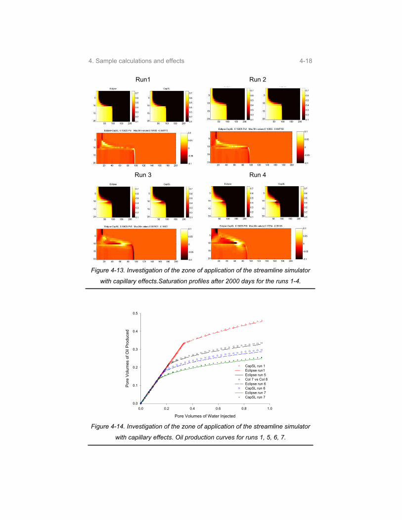
4. Sample calculations and effects 4-18
Run1 Run 2
Run 3 Run 4
Figure 4-13. Investigation of the zone of application of the streamline simulator
with capillary effects.Saturation profiles after 2000 days for the runs 1-4.
Pore Volumes of Water Injected
0.0 0.2 0.4 0.6 0.8 1.0
Por
e V
olum
es o
f Oil
Pro
duce
d
0.0
0.1
0.2
0.3
0.4
0.5
CapSL run 1Eclipse run1Eclipse run 5Col 7 vs Col 8 Eclipse run 6CapSL run 6Eclipse run 7CapSL run 7
Figure 4-14. Investigation of the zone of application of the streamline simulator
with capillary effects. Oil production curves for runs 1, 5, 6, 7.
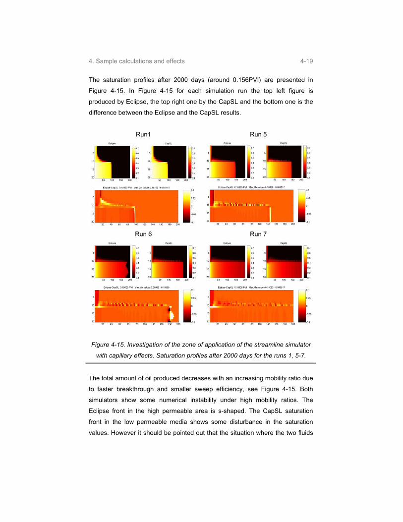
4. Sample calculations and effects 4-19
The saturation profiles after 2000 days (around 0.156PVI) are presented in
Figure 4-15. In Figure 4-15 for each simulation run the top left figure is
produced by Eclipse, the top right one by the CapSL and the bottom one is the
difference between the Eclipse and the CapSL results.
Run1 Run 5
Run 6 Run 7
Figure 4-15. Investigation of the zone of application of the streamline simulator
with capillary effects. Saturation profiles after 2000 days for the runs 1, 5-7.
The total amount of oil produced decreases with an increasing mobility ratio due
to faster breakthrough and smaller sweep efficiency, see Figure 4-15. Both
simulators show some numerical instability under high mobility ratios. The
Eclipse front in the high permeable area is s-shaped. The CapSL saturation
front in the low permeable media shows some disturbance in the saturation
values. However it should be pointed out that the situation where the two fluids
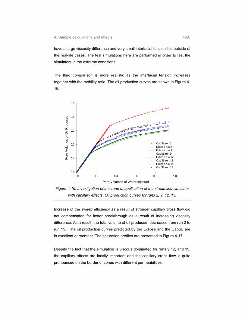
4. Sample calculations and effects 4-20
have a large viscosity difference and very small interfacial tension lies outside of
the real-life cases. The test simulations here are performed in order to test the
simulators in the extreme conditions.
The third comparison is more realistic as the interfacial tension increases
together with the mobility ratio. The oil production curves are shown in Figure 4-
16.
Pore Volumes of Water Injected
0.0 0.2 0.4 0.6 0.8 1
Por
e V
olum
es o
f Oil
Pro
duce
d
.00.0
0.1
0.2
0.3
0.4
0.5
CapSL run 2Eclipse run 2Eclipse run 9CapSL run 9Eclipse run 12CapSL run 12Eclipse run 15CapSL run 15
Figure 4-16. Investigation of the zone of application of the streamline simulator
with capillary effects. Oil production curves for runs 2, 9, 12, 15.
Increase of the sweep efficiency as a result of stronger capillary cross flow did
not compensated for faster breakthrough as a result of increasing viscosity
difference. As a result, the total volume of oil produced decreases from run 2 to
run 15. The oil production curves predicted by the Eclipse and the CapSL are
in excellent agreement. The saturation profiles are presented in Figure 4-17.
Despite the fact that the simulation is viscous dominated for runs 9,12, and 15,
the capillary effects are locally important and the capillary cross flow is quite
pronounced on the border of zones with different permeabilities.

4. Sample calculations and effects 4-21
Run 2 Run 9
Run 12 Run 15
Figure 4-17. Investigation of the zone of application of the streamline simulator
with capillary effects. Saturation profiles after 2000 days for the runs 2, 9, 12,
15.
In Figure 4-17 for each simulation run the top left figure is produced by Eclipse,
the top right one by the CapSL and the bottom one is the difference between
the Eclipse and the CapSL results.
Finally, run 4 is modified to include the gravitational forces and represents the
vertical cross-section of a reservoir. The oil density is set to 800 kg/m3, the
water density to 1000 kg/m3. The saturation profiles predicted by the Eclipse
and the CapSL are presented in Figure 4-18.
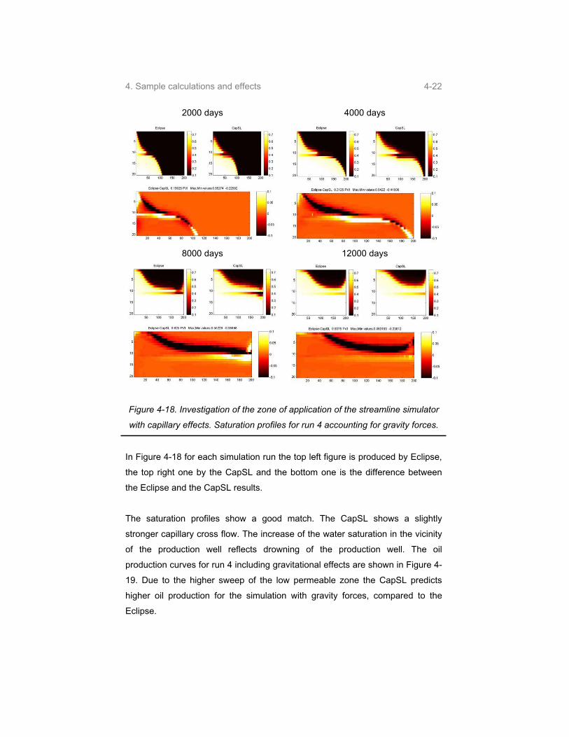
4. Sample calculations and effects 4-22
2000 days 4000 days
8000 days 12000 days
Figure 4-18. Investigation of the zone of application of the streamline simulator
with capillary effects. Saturation profiles for run 4 accounting for gravity forces.
In Figure 4-18 for each simulation run the top left figure is produced by Eclipse,
the top right one by the CapSL and the bottom one is the difference between
the Eclipse and the CapSL results.
The saturation profiles show a good match. The CapSL shows a slightly
stronger capillary cross flow. The increase of the water saturation in the vicinity
of the production well reflects drowning of the production well. The oil
production curves for run 4 including gravitational effects are shown in Figure 4-
19. Due to the higher sweep of the low permeable zone the CapSL predicts
higher oil production for the simulation with gravity forces, compared to the
Eclipse.

4. Sample calculations and effects 4-23
Pore Volumes of Water Injected
0.0 0.2 0.4 0.6 0.8 1.0
Por
e V
olum
es o
f Oil
Pro
duce
d
0.0
0.1
0.2
0.3
0.4
0.5
0.6
CapSL run4Eclipse run 4Eclipse run 4 with gravityCapSL run 4 with gravity
Figure 4-19. Investigation of the zone of application of the streamline simulator
with capillary effects. Oil production curves for run 4 with and without gravity.
Based on the comparison of these test runs the following conclusions may be
produced:
The CapSL makes it possible to simulate displacements with capillary
effects and to obtain the predictions comparable to the industry-standard
reservoir simulator Eclipse 100, using 5 to 10 times less pressure
updates;
The CapSL is applicable to the full test range of the mobility ratios from
0.89 to 17.78, representing the displacements from favorable to highly
unfavorable regimes;
The CapSL is applicable to the full test range of the capillary forces. The
capillary forces have been tested in the range of the interfacial tension
values from 0 mN/m, representing the tracer flow, to 72 mN/m;
The test cases with high mobility ratios without capillary forces result in
numerical problems in both simulators, such as numerical instabilities on
the viscous or capillary enhanced displacement fronts;
More realistic simulation cases are better handled by both simulators and
the predictions obtained are more comparable. For example, the
numerical instabilities decrease when the surface tension is non-zero for
the fluids with large viscosity difference;

4. Sample calculations and effects 4-24
Both simulators predicts water coning in the vicinity of the production well
for the simulation with gravity and capillary effects.
4.3. Laboratory scale simulations
In this section the CapSL and the Eclipse simulations are compared to the
experimental data. The laboratory data, the relative permeability and the
Leverett function curves as well as the sketches of the laboratory set-up were
kindly provided by Dr. Yildiray Cinar and Acting Assistant Professor Kristian
Jessen, SUPRI-C, Department of Petroleum Engineering, Stanford University.
The full description of the experiments may be found in Cinar et al. [23]. The lab
scale experiments are performed using two kinds of glass beads packed and
sealed between two plastic blocks. The experiment is performed using four
different layouts of the glass beads models as shown in figure 4-20.
z
x
y33cm
8cm0.6 cm
(a) Vertical model with reduced gravity effects
Low-permeability layer, k = 52 D
High-permeability layer, k = 190 D
(c) Horizontal model with gravity effects
33cm0.6 cm
8cm
(d) Long horizontal model with gravity effects
53cm
0.6 cm
8cm
(b) Gravity-stabilized horizontal model
33cm8cm 0.6 cm
Figure 4-20. Layouts of the glass beads models.
The glass beads represented with the white color in Figure 4-20 have the
diameter of 0.05cm. The permeability of this layer is 190D. The glass beads
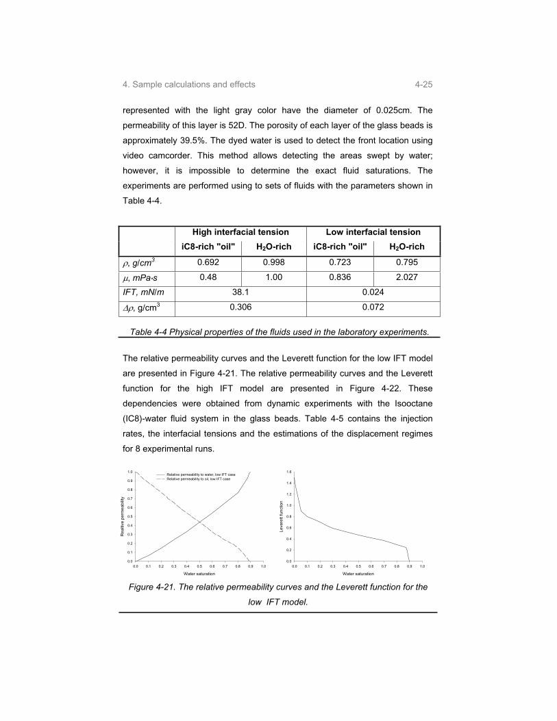
4. Sample calculations and effects 4-25
represented with the light gray color have the diameter of 0.025cm. The
permeability of this layer is 52D. The porosity of each layer of the glass beads is
approximately 39.5%. The dyed water is used to detect the front location using
video camcorder. This method allows detecting the areas swept by water;
however, it is impossible to determine the exact fluid saturations. The
experiments are performed using to sets of fluids with the parameters shown in
Table 4-4.
High interfacial tension Low interfacial tension
iC8-rich "oil" H2O-rich iC8-rich "oil" H2O-rich
, g/cm3 0.692 0.998 0.723 0.795
, mPa*s 0.48 1.00 0.836 2.027
IFT, mN/m 38.1 0.024
, g/cm3 0.306 0.072
Table 4-4 Physical properties of the fluids used in the laboratory experiments.
The relative permeability curves and the Leverett function for the low IFT model
are presented in Figure 4-21. The relative permeability curves and the Leverett
function for the high IFT model are presented in Figure 4-22. These
dependencies were obtained from dynamic experiments with the Isooctane
(IC8)-water fluid system in the glass beads. Table 4-5 contains the injection
rates, the interfacial tensions and the estimations of the displacement regimes
for 8 experimental runs.
Water saturation
0.0 0.1 0.2 0.3 0.4 0.5 0.6 0.7 0.8 0.9 1.0
Rea
ltive
per
mea
bilit
y
0.0
0.1
0.2
0.3
0.4
0.5
0.6
0.7
0.8
0.9
1.0Relative permeability to water, low IFT caseRelative permeability to oil, low IFT case
Water saturation
0.0 0.1 0.2 0.3 0.4 0.5 0.6 0.7 0.8 0.9 1.0
Leve
rett
func
tion
0.0
0.2
0.4
0.6
0.8
1.0
1.2
1.4
1.6
Figure 4-21. The relative permeability curves and the Leverett function for the
low IFT model.
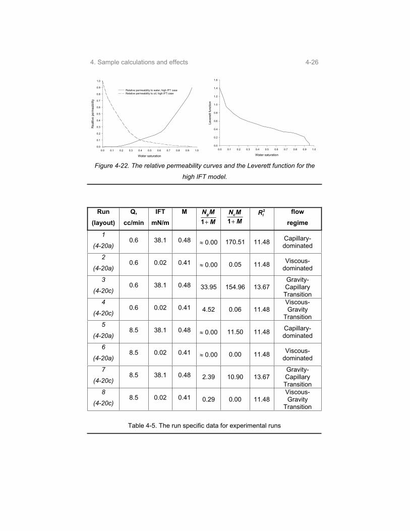
4. Sample calculations and effects 4-26
Water saturation
0.0 0.1 0.2 0.3 0.4 0.5 0.6 0.7 0.8 0.9 1.0
Rea
ltive
per
mea
bilit
y
0.0
0.1
0.2
0.3
0.4
0.5
0.6
0.7
0.8
0.9
1.0
Relative permeability to water, high IFT caseRelative permeability to oil, high IFT case
Water saturation
0.0 0.1 0.2 0.3 0.4 0.5 0.6 0.7 0.8 0.9 1.0
Leve
rett
func
tion
0.0
0.2
0.4
0.6
0.8
1.0
1.2
1.4
1.6
Figure 4-22. The relative permeability curves and the Leverett function for the
high IFT model.
Run
(layout)
Q,
cc/min
IFT
mN/m
M
1
gN M
M 1cN MM
2
lR flow
regime
1
(4-20a)0.6 38.1 0.48 0.00 170.51 11.48 Capillary-
dominated
2
(4-20a)0.6 0.02 0.41 0.00 0.05 11.48 Viscous-
dominated
3
(4-20c)0.6 38.1 0.48 33.95 154.96 13.67
Gravity-CapillaryTransition
4
(4-20c)0.6 0.02 0.41 4.52 0.06 11.48
Viscous-Gravity
Transition5
(4-20a)8.5 38.1 0.48 0.00 11.50 11.48 Capillary-
dominated
6
(4-20a)8.5 0.02 0.41 0.00 0.00 11.48 Viscous-
dominated
7
(4-20c)8.5 38.1 0.48 2.39 10.90 13.67
Gravity-CapillaryTransition
8
(4-20c)8.5 0.02 0.41 0.29 0.00 11.48
Viscous-Gravity
Transition
Table 4-5. The run specific data for experimental runs
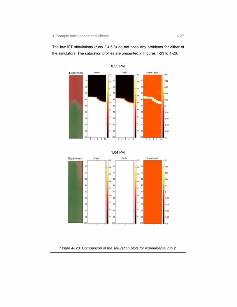
4. Sample calculations and effects 4-27
The low IFT simulations (runs 2,4,6,8) do not pose any problems for either of
the simulators. The saturation profiles are presented in Figures 4-23 to 4-26.
0.55 PVI
1.04 PVI
Figure 4- 23. Comparison of the saturation plots for experimental run 2.

4. Sample calculations and effects 4-28
0.15 PVI
1.39 PVI
Figure 4-24. Comparison of the saturation plots for experimental run 4.
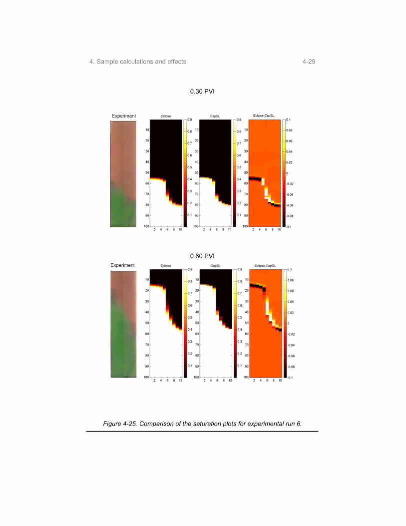
4. Sample calculations and effects 4-29
0.30 PVI
0.60 PVI
Figure 4-25. Comparison of the saturation plots for experimental run 6.
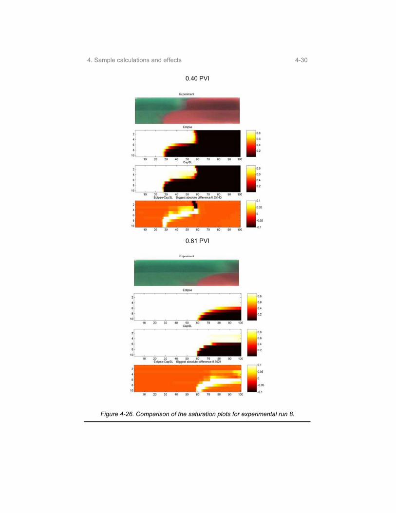
4. Sample calculations and effects 4-30
0.40 PVI
0.81 PVI
Figure 4-26. Comparison of the saturation plots for experimental run 8.

4. Sample calculations and effects 4-31
Basing on Figures 4-23 to 4-26 it may be concluded that both simulators
capture essential features of the displacement profile. The difference between
the simulation and the experimental results for the vertical layout of the
experimentation setup may be due to the wall effects. The Eclipse saturation
front is typically slightly more affected by the numerical dispersion. The oil
production curves are presented in Figures 4-27 to 4-30.
Pore volumes of water injected
0.0 0.1 0.2 0.3 0.4 0.5 0.6 0.7 0.8 0.9 1.0 1.1 1.2 1.3 1.4 1.5 1.6
Por
e vo
lum
es o
f oil
prod
uced
0.0
0.2
0.4
0.6
0.8
1.0ExperimentCapSLEclipse
Figure 4-27. Oil production curves for experimental run 2.
Pore volumes of water injected
0.0 0.1 0.2 0.3 0.4 0.5 0.6 0.7 0.8 0.9 1.0 1.1 1.2 1.3 1.4 1.5 1.6
Por
e vo
lum
es o
f oil
prod
uced
0.0
0.2
0.4
0.6
0.8
1.0ExperimentCapSLEclipse
Figure 4-28. Oil production curves for experimental run 4.

4. Sample calculations and effects 4-32
Pore volumes of water injected
0.0 0.1 0.2 0.3 0.4 0.5 0.6 0.7 0.8 0.9 1.0 1.1 1.2 1.3 1.4 1.5 1.6
Por
e vo
lum
es o
f oil
prod
uced
0.0
0.2
0.4
0.6
0.8
1.0ExperimentCapSLEclipse
Figure 4-29. Oil production curves for experimental run 6.
Pore volumes of water injected
0.0 0.1 0.2 0.3 0.4 0.5 0.6 0.7 0.8 0.9 1.0 1.1 1.2 1.3 1.4 1.5 1.6
Por
e vo
lum
es o
f oil
prod
uced
0.0
0.2
0.4
0.6
0.8
1.0ExperimentCapSLEclipse
Figure 4-30. Oil production curves for experimental run 8.
It may be concluded that both simulators show excellent match with
experimental results. The oil production curves predicted by the CapSL typically
lie slightly closer to the experimental points.

4. Sample calculations and effects 4-33
The high IFT simulations (runs 1, 3, 5, 7) are more complicated to handle.
Moreover, in cases of strong capillary forces small heterogeneities of the glass
beads strongly affect the behavior of the saturation front. The saturation profiles
are presented in Figures 4-31 to 4-34.
0.25 PVI
0.80 PVI
Figure 4-31. Comparison of the saturation plots for experimental run 1.

4. Sample calculations and effects 4-34
0.42 PVI
0.80 PVI
Figure 4-32. Comparison of the saturation plots for experimental run 3.

4. Sample calculations and effects 4-35
0.28 PVI
0.75 PVI
Figure 4-33. Comparison of the saturation plots for experimental run 5.
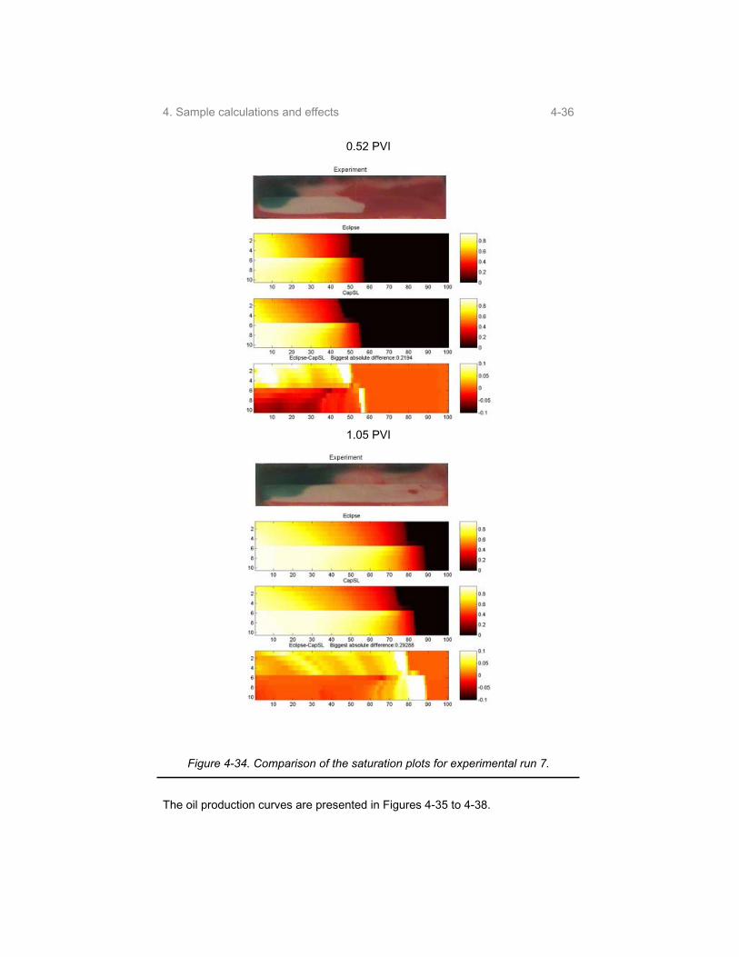
4. Sample calculations and effects 4-36
0.52 PVI
1.05 PVI
Figure 4-34. Comparison of the saturation plots for experimental run 7.
The oil production curves are presented in Figures 4-35 to 4-38.

4. Sample calculations and effects 4-37
Pore volumes of water injected
0.0 0.1 0.2 0.3 0.4 0.5 0.6 0.7 0.8 0.9 1.0 1.1 1.2 1.3 1.4 1.5 1.6
Por
e vo
lum
es o
f oil
prod
uced
0.0
0.2
0.4
0.6
0.8
1.0ExperimentCapSLEclipse
Figure 4-35. Oil production curves for experimental run 1.
Pore volumes of water injected
0.0 0.1 0.2 0.3 0.4 0.5 0.6 0.7 0.8 0.9 1.0 1.1 1.2 1.3 1.4 1.5 1.6
Por
e vo
lum
es o
f oil
prod
uced
0.0
0.2
0.4
0.6
0.8
1.0ExperimentCapSLEclipse
Figure 4-36. Oil production curves for experimental run 3.
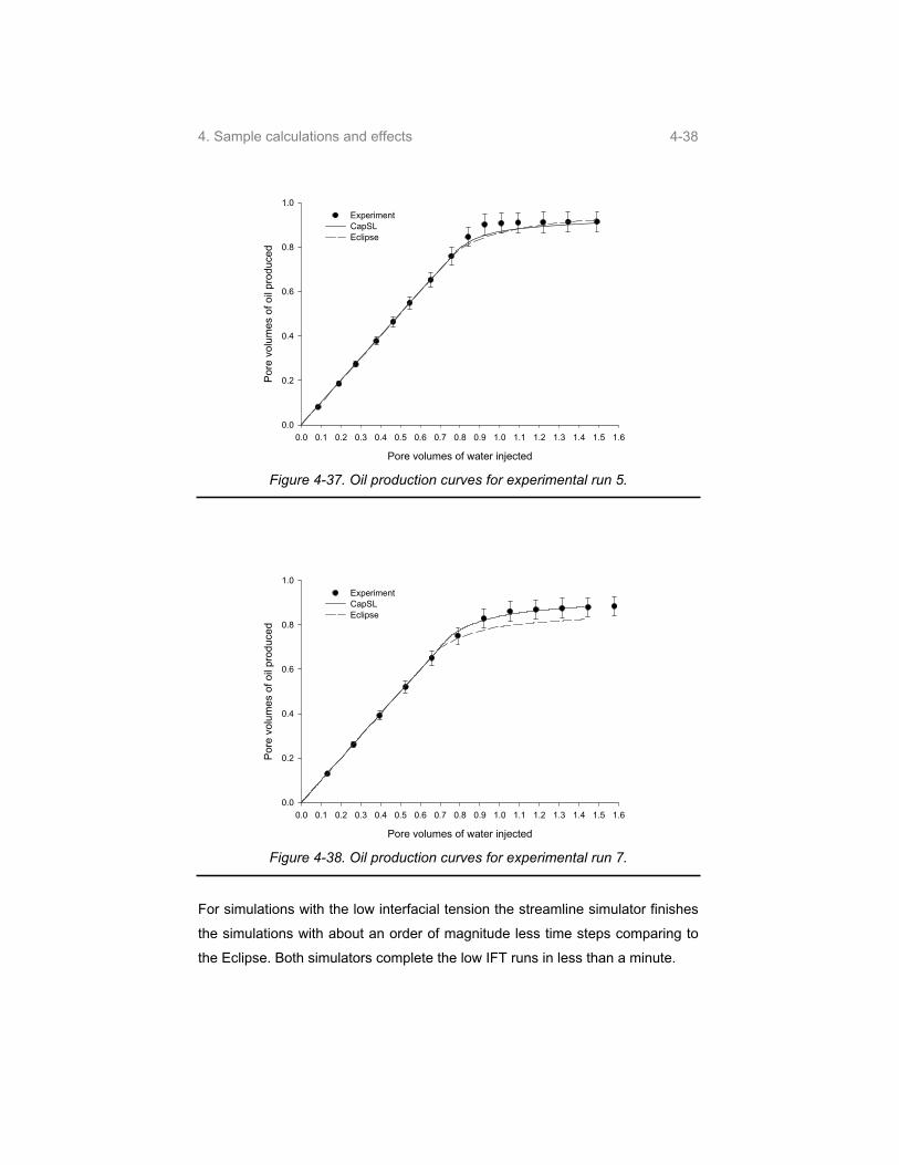
4. Sample calculations and effects 4-38
Pore volumes of water injected
0.0 0.1 0.2 0.3 0.4 0.5 0.6 0.7 0.8 0.9 1.0 1.1 1.2 1.3 1.4 1.5 1.6
Por
e vo
lum
es o
f oil
prod
uced
0.0
0.2
0.4
0.6
0.8
1.0ExperimentCapSLEclipse
Figure 4-37. Oil production curves for experimental run 5.
Pore volumes of water injected
0.0 0.1 0.2 0.3 0.4 0.5 0.6 0.7 0.8 0.9 1.0 1.1 1.2 1.3 1.4 1.5 1.6
Por
e vo
lum
es o
f oil
prod
uced
0.0
0.2
0.4
0.6
0.8
1.0ExperimentCapSLEclipse
Figure 4-38. Oil production curves for experimental run 7.
For simulations with the low interfacial tension the streamline simulator finishes
the simulations with about an order of magnitude less time steps comparing to
the Eclipse. Both simulators complete the low IFT runs in less than a minute.

4. Sample calculations and effects 4-39
The numbers of time steps taken by the CapSL and the Eclipse to complete the
high IFT runs are quite comparable. As a result, the simulation time is about the
same as well. The streamline methodology is designed and is advantageous in
the cases where the main mass transfer is due to the viscous forces. In the
presented high IFT simulations the displacement profile is controlled by the
capillary forces. In case of the strongly capillary dominated displacement the
CapSL performance is entirely controlled by the stability of the corrector step.
Since the corrector step is performed on the finite difference grid, the time step
size of the streamline simulator approaches the time step size of the finite-
difference method. The streamline simulator may become slower due to the
additional, comparing to the finite difference method, streamline tracing
procedure. Moreover, the mapping error increases as well, resulting in large
mass balance errors of several percent. Run 3 is the most difficult for the
streamline simulator and results in the mass balance error of around 7%.
Several streamlines actually looped and returned to the injection well. The loop
back of the streamlines may happen not only for capillary, but for the gravity
simulations as well [18]. Nevertheless, the CapSL and the Eclipse results are in
an excellent agreement. Based on the presented simulations, it may be
concluded that the streamline simulator in its current realization is applicable to
the simulation of the laboratory scale displacements with different displacement
regimes. However, in case of high capillary numbers the application of the
streamline simulator is not beneficial.

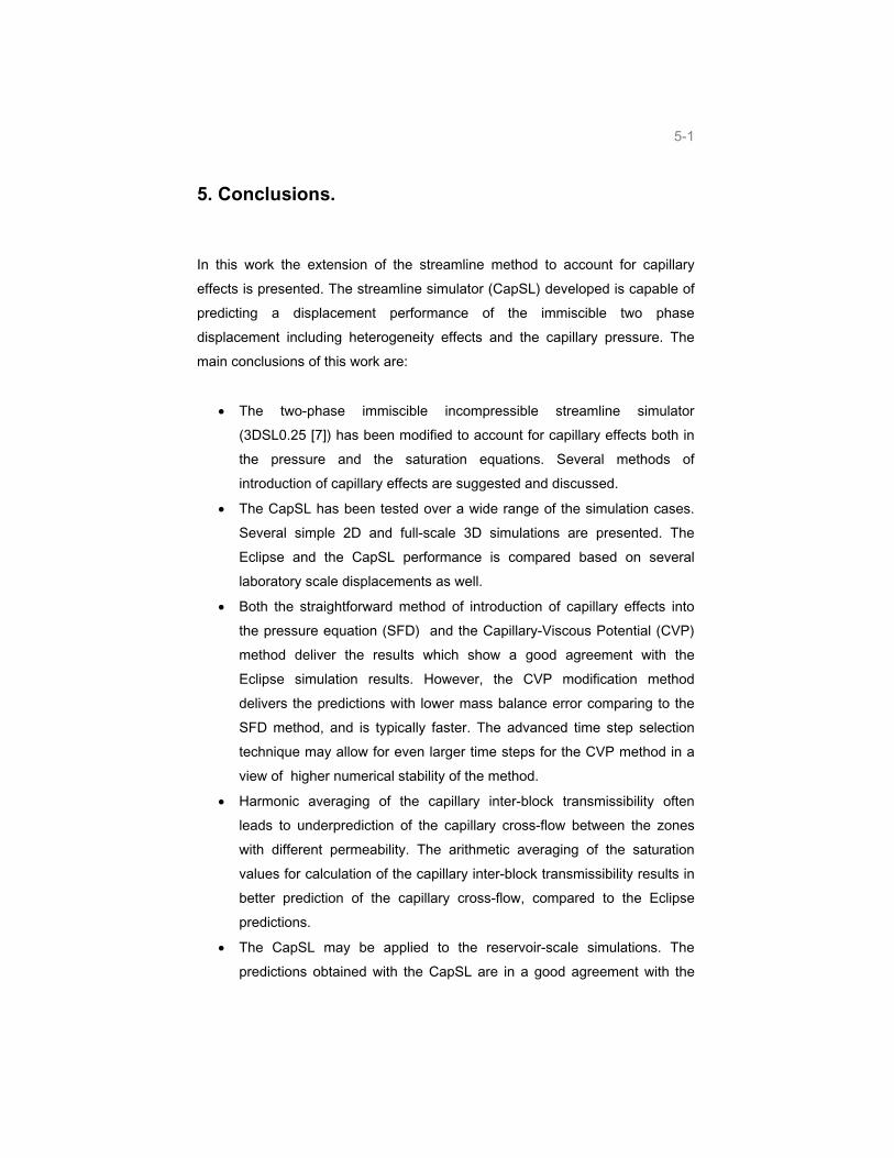
5-1
5. Conclusions.
In this work the extension of the streamline method to account for capillary
effects is presented. The streamline simulator (CapSL) developed is capable of
predicting a displacement performance of the immiscible two phase
displacement including heterogeneity effects and the capillary pressure. The
main conclusions of this work are:
The two-phase immiscible incompressible streamline simulator
(3DSL0.25 [7]) has been modified to account for capillary effects both in
the pressure and the saturation equations. Several methods of
introduction of capillary effects are suggested and discussed.
The CapSL has been tested over a wide range of the simulation cases.
Several simple 2D and full-scale 3D simulations are presented. The
Eclipse and the CapSL performance is compared based on several
laboratory scale displacements as well.
Both the straightforward method of introduction of capillary effects into
the pressure equation (SFD) and the Capillary-Viscous Potential (CVP)
method deliver the results which show a good agreement with the
Eclipse simulation results. However, the CVP modification method
delivers the predictions with lower mass balance error comparing to the
SFD method, and is typically faster. The advanced time step selection
technique may allow for even larger time steps for the CVP method in a
view of higher numerical stability of the method.
Harmonic averaging of the capillary inter-block transmissibility often
leads to underprediction of the capillary cross-flow between the zones
with different permeability. The arithmetic averaging of the saturation
values for calculation of the capillary inter-block transmissibility results in
better prediction of the capillary cross-flow, compared to the Eclipse
predictions.
The CapSL may be applied to the reservoir-scale simulations. The
predictions obtained with the CapSL are in a good agreement with the
5. Conclusions 5-2
Eclipse. The CapSL delivers the predictions around 10 times faster
compared to the Eclipse. The speed-up factor increases with increase of
the simulation grid size.
For the 3D simulation the CapSL predictions are in accordance with the
displacement regime estimated by Bedrikovetsky and Zhou et al.
dimensionless groups. The total oil production predicted by the CapSL
was not affected by the capillary forces. However, the local displacement
profiles for the simulation including and neglecting capillary effects were
different. The total oil production predicted by the Eclipse was affected by
the capillary forces. The Eclipse simulation without capillary effects
resulted in lower oil production due to the higher numerical dispersion.
The CapSL is less affected by the numerical dispersion in both the small-
scale and the reservoir scale simulations. As a result fine features of the
displacement front are better captured.
The effects of alternated wet reservoirs are fully accounted for in the
CapSL.
The zone of application of the streamline simulator has been expanded
to the areas of local or global capillary dominated displacements
compared to prior art streamline simulation methods.
Comparison of the CPU time is not entirely fair for neither the CapSL nor
the Eclipse. The CapSL is a research code which is not optimised to
deliver the ultimate performance. However, the Eclipse 100 is used in the
least dispersed, but in a lot of cases, the slowest IMPES formulation. An
adaptive implicit solution scheme delivers faster simulation result without
loosing too much accuracy.
For the simulation of those heterogeneous reservoirs with strong
capillary domination on the reservoir scale the current streamline
methods do no provide serious advantages over the finite difference
simulators. Performance of the CapSL is restricted by the performance of
the corrector step on the finite difference grid.
The future research on the streamline methods may include:
1) Advanced time step selection routines. The currently applied routines
are rather simplistic and may result in non-optimal time steps. The

5. Conclusions 5-3
time steps must be chosen in the way to ensure the scheme stability.
On the other hand, over-restricting the time step size results in the
slower scheme, affected by the numerical dispersion associated with
mapping;
2) An application of advanced streamline tracing and mapping routines
[48] may facilitate decreasing both simulation time and the numerical
error;
3) Handling advanced grids;
4) Advanced well equations;
5) Introduction of capillary effects into two and three phase
compositional streamline simulators.


6-1
Nomenclature
Symbols
c Coefficient
C sm2kg-1 Capillary inter-block transmissibility for the SFD method
Cn Courant number
D m Depth
E Error
f Fractional flow function
F Function
g m/c2 Gravitational constant
H, h m Height
J Leverett function
k m2 Permeability
L, l m Length
M Mobility ratio
m, n Coefficients in the vanGenuchten model
n m-2 Number of capillaries per unit area (chapter 1)
N sm2kg-1 Capillary inter-block transmissibility for the CVP method
Dimensionless parameter (chapter 3)
P Pa Pressure
Q, q m3/s Flow rate
r m Radius
R Shape factor
S Saturation
t s Time
T sm2kg-1 Transfer function (chapter 1)
Inter-block transmissibility (chapter 2)

Nomenclature 6-2
U m/s Velocity
V m3 Volume
x, y, z Axes
Unknowns (section 1.3.2)
Greek symbols
m Distance from the block center to the interface
Dimensionless parameters
Porosity
Pa The porous media dependent term of the capillary pressure
Ratio of the gravity mobility to the total mobility
Pa Capillary - viscous potential
Pa s Mobility
Average value
P Viscosity
Wettability angle
kg/m3 Density
N/m Interfacial tension
s Time of flight
Capillary - viscous potential multiplier
Indexes
av Average
c Capillary, critical (in formula 1.22)
g Gravitational, gravity
i,j, k One of the phases or axes
o Oil

Nomenclature 6-3
or Oil residual
r Relative
rowi Relative oil at initial water
rwor Relative water at oil residual
s Surface
t Total
v Viscous
w Wetting
wi Water initial


7-1
References
1. Adamson, A.W. Phsyical Chemistry of Surfaces. John Wiles & Sons,
New York, USA. 1997.
2. Agarwal, B., and Blunt, M.J. Streamline Based Method With Full-Physics
Forward Simulation for History-Matching Performance Data of a North
Sea Field. SPE 84952 in SPEJ June, pp. 171-180. 2003.
3. Al-Huthali, A.H., and Datta-Gupta, A. Streamline Simulation of Water
Injection in Naturally Fractured Reservoirs. SPE 89443 presented at the
2004 SPE/DOE Symposium on Improved Oil Recovery, Tulsa, USA.
2004.
4. Amyx, J.W., Bass, D.M., and Whiting, R.L. Petroleum Reservoir
Engineering. McGraw-Hill, New York, USA. 1960.
5. Aziz, K., and Settari, A. Petroleum reservoir simulation. Elsevier applied
science publishers, New York, USA. 1979.
6. Basniev, K.S., Kochina, I.N., and Maksimov, V.M. Underground
hydromechanics (Podzemnaja gidromechannica). In Russian. Moscow,
Russia. 1993.
7. Barenblatt, G.I., Entov, V.M., Ryzhik, V.M. Theory of fluid flows through
natural rocks. Kluwer Academic publisher, Netherlands. 1990.
8. Batycky, R.P. A Three-Dimensional Two-Phase Field Scale Streamline
Simulator. Ph.D. Thesis, Department of Petroleum Engineering, School
of Earth Science, Stanford University, Stanford, California, USA. 1997.
9. Bedrikovetsky, P.G. Mathematical Theory of Oil and Gas Recovery With
Application to ex-USSR Oil and Gas Fields. Kluwer Academic
Publishers, Netherlands. 1993.
10. Bedrikovetsky, P.G., Magarshak, T.O., and Shapiro A.A. 3D Analytical
Model for Displacement of Oil Using Horizontal Wells. SPE 26996

References 7-2
presented at III Latin American / Caribbean Confernce held in Buenos
Areas, Argentina. 1994.
11. Bedrikovetsky, P.G. New Mathematical Model for EOR Displacements
Honoring Oil Ganglia. SPE 38892 presented at the SPE Annual
Technical Conference and Exhibition, San Antonio, Texas, USA. 1997.
12. Bedrikovetsky, P.G. WAG Displacemetns of Oil-Condensates Accounting
for Hydrocarbon Ganglia. Transport in Porous Media, Vol.52, pp. 229-
266. 2003.
13. Bedrikovetsky, P.G. Analytical Model for the Waterflood Honoring
Capillary Pressure. SPE 36130, presented at the Fourth Latin and
Caribbean Petroleum Engineering Conference held in Port-of-Spain,
Trinidad and Tobago. 1996.
14. Berenblyum, R.A., Shapiro, A.A., Jessen, K., Stenby, E.H., and Orr, F.M.
Jr. Black Oil Streamline Simulator With Capillary Effects. SPE 84037,
presented at the SPE Annual Technical Conference and Exhibition held
in Denver, Colorado, USA. 2003.
15. Berenblyum, R.A., Shapiro, A.A., Stenby E.H. A Method For Simulating A
Multiphase Flow. Patent Application PA 2003 01844, Denmark. 2003.
16. Berre, I., Dahle, H.K., Karlsen, K.H., and Nordhaug, H.F. A Streamline
Front Tracking Method for Two- and Three-Phase Flow Including
Capillary Forces. Mathematics Subject Classification, pp 1-13. 2000.
17. Blair, P.M., and Weinlaug, C.F. Solution of Two-Phase Flow Problems
Using Implicit Difference Equations. SPE 2185, Presented at 43rd Annual
Fall Meeting, Houston, USA. 1969.
18. Blunt, M.J., Lui, K., Thiele, M.R. A Generalized Streamline Method to
Predict Reservoir Flow. Petroleum Geoscience, vol. 2, pp. 259-269.
1996.
19. Blunt, M.J. Flow in porous media – pore-network models and multiphase
flow. Current Opinion in Colloid & Interface Science, vol. 6, pp 197-207.
2001.

References 7-3
20. Bratvedt, F., Bratvedt, K., Buchholz, C.F., Gimse, T., Holden, H., Holden,
L., and Risebro, N.H. Frontline and Frontsim: two full scale, two-phase,
black oil reservoir simulators based on front tracking. Surveys on
Mathematics for Industry, vol. 3, pp. 63-78. 1993.
21. Bratvedt, F., Gimse, T., and Tegnander, C. Streamline Computations for
Porous Media Flow Including Gravity. Transport in Porous Media, vol. 25,
pp. 63-78. 1996.
22. Buckley, S.E., and Leverett, M.C. Mechanisms of Fluid Displacement in
Sands. Petroleum Technology, May, pp107-116. 1941.
23. Cinar, Y., Jessen, K., Juanes, Berenblyum, R., and Orr, F.M. An
experimental and Numerical Investigation of Crossflow Effects in Two-
Phase Displacements. SPE 90568, to be presented at the SPE Annual
Technical Conference and Exhibition, Houston, USA. 2004.
24. Christie, M.A., and Blunt, M.J. Tenth SPE Solution Project: A comparison
of Upscaling Techniques. SPE72469 in SPE Reservoir Evaluation and
Engineering, August, pp. 308-317. 2001.
25. Coats, K.H. Implicit Compositional Simulation of Single-Porosity and
Dual-Porosity Reservoirs. SPE 18427, presented at SPE Symposium On
Reservoir Simulation, Huston, USA. 1989.
26. Coats, K.H. A Note on IMPES and Some IMPES-Based Simulation
Models. SPE 65092 in SPE Journal, vol. 5, pp. 245-251. 2000.
27. Coats, K.H. IMPES Stability: The CFL Limit. SPE 66345, presented at
SPE Reservoir Simulation Symposium, Houston, USA. 2001
28. Coats, K.H. IMPES Stability: The Stable Step. SPE 69225, presented at
SPE Reservoir Simulation Symposium, Huston, USA. 2001.
29. Coats, K.H. IMPES Stability: Selection of Stable Timesteps. SPE 84924
in SPEJ, June, pp. 187-187. 2003.
30. Crane, M., Bratvedt, F., Bratvedt, K., Childs, P., and Olufsen, R. A Fully
Compositional Streamline Simulator. SPE 63156 presented at SPE
Annual Technical Conference and Exhibition, Dallas, Texas, USA. 2000.

References 7-4
31. Darcy, H. The public fountains in the Town of Dijon, V. Dalmont, Paris,
France. 1856
32. Datta-Gupta, A., and King, M.J. A Semianalytic Approach to Tracer Flow
Modeling in Heterogeneous Permeable Media. Advances in Water
Resources, vol. 18, pp. 9-24. 1995.
33. Di Donato, G., Huang, W., and Blunt, M. Streamline-Based Dual Porosity
Simulation of Fractured Reservoirs. SPE 84036 presented at SPE
Annual Technical Conference and Exhibition, Denver, Colorado, USA.
2003.
34. Dullien, F.A.L. Porous media. Fluid Transport and Pore Structure.
Academic Press, New York, USA. 1979.
35. Emanuel, S., and Milliken, W.J. History Matching Finite Difference
Models With 3D Streamlines. SPE 49000 presented at SPE Annual
Technical Conference and Exhibition, New Orleans, Louisiana, USA.
1998.
36. Farkas, E. Adaptice Implicit Volume Balance Techniques. SPE 25273
presented at 12th SPE Symposium on Reservoir Evaluation, New
Orleans, Louisiana, USA. 1993.
37. Higgins, R.V., and Leighton, A.J. Performance of Five-spot Water Floods
in Stratified Reservoirs Using Streamlines, SPE 57 in Trans. AIME, pp.1-
12. 1961.
38. Higgins, R.V., and Leighton, A.J. A Computer Method to Calculate Two-
Phase Flow in Amy Irregular Bounded Porous Medium. SPE 243,
presented at SPE Annual California Regional Meeting, USA. 1962.
39. Higgins, R.V., and Leighton, A.J. Computer Prediction of Water Drive of
Oil and Gas Mixture Through Irregularly Bounded Porous Media – Three-
Phase Flow. SPE 283, presented at SPE production reservoir
Symposium, Tulsa, Oklahoma, USA1962.
40. Ichiro, O., Datta-Gupta, A., and King, M.J. Time step selection during
streamline simulation via transverse flux correction. SPE 79688,
References 7-5
presented at 2003 SPE reservoir simulation symposium, Huston, USA.
2003.
41. Jessen, K., Wang, Y., Ermakov, P., Zhu, J., and Orr, F.M. Fast,
Approxmate Soilutions for 1D Mulitcomponent Gas-Injection Problems.
SPE 74700 in SPEJ, December, pp. 442-451. 2001.
42. Jessen, K., and Orr, F.M. Compositional Streamline Simulation. SPE
77379 presented at SPE Annual Technical Conference and Exhibition,
San Antonio, Texas, USA. 2002.
43. Jessen, K., and Orr, F.M. Gas Cycling and the Development of Miscibilty
in Condensate Reservoirs. SPE 84070 presented at SPE Annual
Technical Conference and Exhibition, Denver, Colorado, USA. 2003.
44. Jessen, K., and Orr, F.M. Gravity segregation and Compositional
Streamline Simulation. SPE 89448, presented at SPE/DOE symposium
on Improved Oil Recovery, Tulsa, Oklahoma, USA. 2004.
45. Killough, J.E. and Kossack, C.A. Fifth Comparative Solution project:
Evaluation of Miscible Flood Simulators. SPE 16000 presented at Ninth
SPE Symposium on Reservoir Simulation, San Antonio, Texas, USA.
1987.
46. King, M.J., and Datta-Gupta, A. Streamline Simulation: A current
perspective. In Situ, vol. 22(1), pp. 91-140. 1998.
47. Leverett, M.C. Capillary behavior in Porous Solids. Trans. AIME. 1941.
48. Mallison, B.T., Gerritsen, M.G, and Matringe S.F. Improved Mappings for
Streamline-Based Simulation. SPE 89352 presented at the 2004
SPE/DOE Symposium on Improved Oil Recovery, Tulsa, Oklahoma,
USA. 2004.
49. Marcell-De Silva, J., and Dawe, R.A. Effects of Permeability and
Wettability Heterogeneities on Flow in Porous Media. SPE 81164
presented at SPE Latin American and Caribbean Petroleum Engineering
Conference, Port-of-Spain, Trinidad, West Indies. 2003.

References 7-6
50. Martin, J.C., and Wegner, R.E. Numerical Solution of Multiphase, Two-
Dimensional Incompressible Flow Using Stream-Tube Relationships.
SPE 7140 in Trans. AIME, October, pp. 313-323. 1979
51. Matanga, G.B. Stream Functions in Three-Dimensional Groundwater
Flow. Water resources Research, vol. 29(9), pp 3125-3133. 1993.
52. Mattax, C.C., and Dalton, R.L. Reservoir Simulation. SPE Monogram
Series. SPE, Richardson, Texas, USA. 1990.
53. Milliken, W.J., Emanuel, A.S., and Chakravarty, A. Application of 3D
Streamline Simulation To Assist History Matching. SPE 74712,
presented at SPEREE December, pp. 502-508. 2001.
54. Muskat, M. Flow of Homogeneous Fluids. McGraw-Hill, Boston, USA.
1937.
55. Peaceman, D.W. Fundamentals of numerical reservoir simulation.
Elsevier, New York, USA. 1977
56. Peaceman, D.W. Interpretation of Well-Block Properties in Numerical
Reservoir Simulation with Nonsquare Grid Blocks and Anisotropic
Permeability. SPE 10528 in SPEJ, June, pp. 531-569. 1983
57. Pollock, D.W. Semianalytical Computation of Path Lines for Finite-
Difference Models. Ground Water, vol.26(6), pp. 743-750. 1988.
58. Rapoport, L.A., and Leas, W.J. Properties of Linear Waterfloods.
Petroleum Transactions AIME, vol.198, pp. 139-148. 1953.
59. Renard, G. A 2D Reservoir Streamtube EOR Model With Periodical
Automatic Regeneration of Streamlines. In Situ, vol. 14(2), pp. 175-200.
1990.
60. Rodriguez, P.G., Segura, M.K., and Moreno, F.J.M. Streamline
methodology using an efficient operator splitting for accurate modeling of
capillary and gravity effects. SPE 79693, presented at SPE Reservoir
Simulation Symposium, Houston, USA. 2003.

References 7-7
61. Russell, T.F. Stability Analysis and Switching Criteria for Adaptive Implicit
Methods Based on the CFL condition. SPE 18416 presented at SPE
Symposium on Reservoir Simulation, Houston, Texas, USA. 1989.
62. Schlumberger GeoQuest. Eclipse 100 Technical Description. 2003.
63. Schlumberger GeoQuest. Eclipse 300 Reference Manual. 2003.
64. Schlumberger GeoQuest. FrontSim Technical Description. 2003.
65. Seto, C.J., Jessen, K., and Orr, F.M. Compositional Streamline
Simulation of Field Scale Condensate Vaporization by Gas Injection.
SPE 79690 presented at SPE Reservoir Simulation Symposium,
Houston, Texas, USA. 2003.
66. Shapiro, A.A, and Stenby, E.H. Factorization of Transport Coefficients in
Macroporous Media. Transport in Porous Media, vol. 41, pp. 305-323.
2000.
67. Spivak, A., and Coats, K.H. Numerical Simulation of Coning Using
Implicit Production Terms. SPE 2595 in SPEJ, September, pp. 257-267.
1970.
68. Thiele, M.R. Modeling Multiphase Flow in Heterogeneous Media Using
Streamtubes. PhD dissertation, Stanford University, Dept. of Petroleum
Engineering, Stanford, California, USA. 1994.
69. Thiele, M.R., Batycky, R.P., Blunt, M.J., and Orr, F.M. Jr. Simulating
Flow in Heterogeneous Media Using Streamtubes and Streamlines. SPE
27834 in SPE Reservoir Engineering, vol. 10(1), pp. 5-12. 1996.
70. Thiele, M. R., Batycky, R.P., and Blunt, M.J. A Streamline-Based 3D
Field-Scale Compositional Reservoir Simulator. SPE 38889 presented at
SPE Annual Technical Conference and Exhibition, San Antonio, Texas,
USA. 1997.
71. Thiele, M.R. Streamline Simulation. 6th international forum on Reservoir
Simulation, Austria. 2001.

References 7-8
72. Thiele, M.R., and Batycky, R.P. Water Injection Optimization Using a
Streamline-Based Workflow. SPE 84080 presented at SPE Annual
Technical Conference and Exhibition, Denver, Colorado, USA. 2003.
73. Thomas, G.W., and Thurnau, D.H. Reservoir Simulation Using an
Adaptive Implicit Method. SPE 10120 presented at the 56th Annual Fall
Technical Conference and Exhibition of the SPE of AIME, San Antonio,
Texas, USA. 1981.
74. Thomas, G.W., and Thurnau, D.H. The Mathematical Basis of the
Adaptive Implicit Method. SPE 10495 presented at the 6th SPE
Symposium in Reservoir Simulation, New Orleans, Louisiana, USA.
1982.
75. Toth, J. Adsorption: Theory, Modeling, and Analysis. Marcel Dekker,
New York, USA. 2002.
76. Trangenstein, J.A. Numerical Analysis of Reservoir Fluid Flow,
Multiphase Flow in Porous Media: Mechanics, Mathematics and
Numerics, Lecture notes in Engineering. Springer Verlag (34).
77. van Genuchten, M.Th. A closed-form Equation for Prediciting the
Hydraulic Conductivity of Unsaturated Soils. Soil Sci. Soc. Am. J., vol.
44, p. 892. 1980.
78. Yan, W., Michelsen, M.L., Stenby, E.H., Berenblyum, R.A., and Shapiro,
A.A. Three-phase Compositional Streamline Simulation and Its
Application to WAG. SPE 89440 presented at the 2004 SPE/DOE
Symposium on Improved Oil Recovery, Tulsa, USA. 2004.
79. Young, L.C., and Russell, T.F. Implementation of an Adaptive Implicit
Method. SPE 25245 presented at 12th SPE Symposium on Reservoir
Simulation, New Orleans, Louisiana, USA. 1993.
80. Zhou, D., Fyaers, F.J., and Orr, F.M. Scaling multiphase flow in simple
heterogeneous porous media. Multiphase Transport in Porous Media,
vol. 265, pp. 25-35. 1993.
The high energy demands in our society pose great challenges if
we are to avoid adverse environmental effects. Increasing energy
efficiency and the reduction and/or prevention of the emission
of environmentally harmful substances are principal areas of focus
when striving to attain a sustainable development. These are the
key issues of the CHEC (Combustion and Harmful Emission Control)
Research Centre at the Department of Chemical Engineering of the
Technical University of Denmark. CHEC carries out research in
fields related to chemical reaction engineering and combustion,
with a focus on high-temperature processes, the formation and
control of harmful emissions, and particle technology.
In CHEC, fundamental and applied research, education and know-
ledge transfer are closely linked, providing good conditions for the
application of research results. In addition, the close collabora-
tion with industry and authorities ensures that the research activ-
ities address important issues for society and industry.
CHEC was started in 1987 with a primary objective: linking funda-
mental research, education and industrial application in an inter-
nationally orientated research centre. Its research activities are
funded by national and international organizations, e.g. the Tech-
nical University of Denmark.
Roman A. Berenblyum
Streamline Simulation with Capillary Effects Applied to Petroleum Engineering Problems
ISBN: 87-91435-08-0


