STRATIFIED ROTATING BOUSSINESQ EQUATIONS …state bifurcation while Rc2 leads to the onset of the...

arX

iv:m

ath-

ph/0

6100

87v2

28

Jan

2007

STRATIFIED ROTATING BOUSSINESQ EQUATIONS IN

GEOPHYSICAL FLUID DYNAMICS: DYNAMIC BIFURCATION

AND PERIODIC SOLUTIONS

CHUN-HSIUNG HSIA, TIAN MA, AND SHOUHONG WANG

Abstract. The main objective of this article is to study the dynamics of thestratified rotating Boussinesq equations, which are a basic model in geophys-ical fluid dynamics. First, for the case where the Prandtl number is greaterthan one, a complete stability and bifurcation analysis near the first criticalRayleigh number is carried out. Second, for the case where the Prandtl num-ber is smaller than one, the onset of the Hopf bifurcation near the first criticalRayleigh number is established, leading to the existence of nontrivial periodicsolutions. The analysis is based on a newly developed bifurcation and stabilitytheory for nonlinear dynamical systems (both finite and infinite dimensional)by two of the authors [16].

1. Introduction

The phenomena of the atmosphere and ocean are extremely rich in its organiza-tion and complexity, and a lot of them cannot be produced by experiments. Thesephenomena involve a broad range of temporal and spatial scales. As we know, boththe atmospheric and oceanic flows are flows under the rotation of the earth. In fact,fast rotation and small aspect ratio are two main characteristics of the large scaleatmospheric and oceanic flows. The small aspect ratio characteristic leads to theprimitive equations, and the fast rotation leads to the quasi-geostrophic equations.These are fundamental equations in the study of atmospheric and oceanic flows;see Ghil and Childress [6], Lions, Temam and Wang [12, 13], and Pedlosky [23].Furthermore, convection occurs in many regimes of the atmospheric and oceanicflows.

A key problem in the study of climate dynamics and in geophysical fluid dy-namics is to understand and predict the periodic, quasi-periodic, aperiodic, andfully turbulent characteristics of large-scale atmospheric and oceanic flows. Stabil-ity/bifurcation theory enables one to determine how different flow regimes appearand disappear as control parameters, such as the Reynolds number, vary. It, there-fore, provides one with a powerful tool to explore the theoretical capability in thepredictability problem. Most studies so far have only considered systems of or-dinary differential equations (ODEs) that are obtained by projecting the PDEsonto a finite-dimensional solution space, either by finite differencing or by truncat-ing a Fourier expansion (see Ghil and Childress [6] and further references there).

Date: August 9, 2018.Key words and phrases. Boussinesq equations, geophysical fluid dynamics, attractor bifurca-

tion, onset of Hopf bifurcation.The work was supported in part by the Office of Naval Research, by the National Science

Foundation, and by the National Science Foundation of China.

1

http://arxiv.org/abs/math-ph/0610087v2

2 C. HSIA, T. MA, AND S. WANG

These were pioneered by Lorenz [14, 15], Stommel [25], and Veronis [27, 28] amongothers, who explored the bifurcation structure of low-order models of atmosphericand oceanic flows. More recently, pseudo-arclength continuation methods havebeen applied to atmospheric (Legras and Ghil [11]) and oceanic (Speich et al. [24]and Dijkstra [5]) models with increasing horizontal resolution. These numericalbifurcation studies have produced so far fairly reliable results for two classes ofgeophysical flows: (i) atmospheric flows in a periodic mid-latitude channel, in thepresence of bottom topography and a forcing jet; and (ii) oceanic flows in a rect-angular mid-latitude basin, subject to wind stress on its upper surface; see amongothers Charney and DeVore [2], Pedlosky [22], Legras and Ghil [11] and Jin andGhil [10] for saddle-node and Hopf bifurcations in the the atmospheric channel, and[20, 1, 8, 9, 19, 24] for saddle-node, pitchfork or Hopf in the oceanic basin.

The main objective of this article is to conduct bifurcation and stability analysisfor the original partial differential equations (PDEs) that govern geophysical flows.This approach should allow us to overcome some of the inherent limitations of thenumerical bifurcation results that dominate the climate dynamics literature up tothis point, and to capture the essential dynamics of the governing PDE systems.

The present article addresses the stability and transitions of basic flows for thestratified rotating Boussinesq equations. These equations are fundamental equa-tions in the geophysical fluid dynamics; see among others Pedlosky [23]. We obtaintwo main results in this article. The first is to conduct a rigorous and completebifurcation and stability analysis near the first eigenvalue of the linearized problem.The second is the onset of the Hopf bifurcation, leading to the existence of periodicsolutions of the model.

The detailed analysis is carried out in two steps. The first is a detailed study ofthe eigenvalue problem for the linearized problem around the basic state. In com-parison to the classical Benard convection problem, the linearized problem here isnon-selfadjoint, leading to much more complicated spectrum, and more complicateddynamics. We derive in particular two critical Rayleigh numbers Rc1 and Rc2 . HereRc1 is the first critical Rayleigh number for the case where the Prandtl number isgreater than one, and Rc2 is the first critical Rayleigh number for the case wherethe Prandtl number is less than one. Moreover, Rc1 leads to the onset of the steadystate bifurcation while Rc2 leads to the onset of the Hopf bifurcation. Both param-eters are explicitly given in terms of the physical parameters. The crucial issueshere include 1) a complete understanding of the spectrum, 2) identification of thecritical Rayleigh numbers, and most importantly 3) the verification of the Principleof Exchange of Stabilities near these critical Rayleigh numbers.

The second step is to conduct a rigorous nonlinear analysis to derive the bifurca-tions at both the critical Rayleigh numbers based on the classical Hopf bifurcationtheory and a newly developed dynamic bifurcation theory by two of the authors.This new dynamic bifurcation theory is centered at a new notion of bifurcation,called attractor bifurcation for dynamical systems, both finite dimensional and infi-nite dimensional, together with new strategies for the Lyapunov-Schmidt reductionand the center manifold reduction procedures. The bifurcation theory has been ap-plied to various problems from science and engineering, including, in particular, theKuramoto-Sivashinshy equation, the Cahn-Hillard equation, the Ginzburg-Landauequation, Reaction-Diffusion equations in Biology and Chemistry, and the Benardconvection problem, the Taylor problem; see [16, 17] and the references therein.

STRATIFIED ROTATING BOUSSINESQ EQUATIONS 3

We remark that the non-selfadjointness of the linearized problem gives rises theonset of the Hopf Bifurcation. We prove that the Hopf bifurcation appears at theRayleigh number Rc2 . As mentioned earlier, the understanding and prediction ofof the the periodic, quasi-periodic, aperiodic, and fully turbulent characteristics oflarge-scale atmospheric and oceanic flows are key issues in the study of climatedynamics and in geophysical fluid dynamics. It is hoped that the study carried outin this article will provide some insights in these important issues.

Also, we would like to mention that rigorous proof of the existence of periodicsolutions for a fluid system is a normally a very difficult task from the mathematicalpoint of view. For instance, with a highly involved analysis, Chen et al. [3] provedthe existence of a Hopf bifurcation in an idealized Fourier space.

The paper is organized as follows. Section 2 gives the basic setting of the problem.Section 3 states the main results. The proofs of the main results occupies theremaining part of the paper: Section 4 recapitulates the essentials of the attractorbifurcation theory, Section 5 is on the eigenanalysis, and Section 6 is on the centralmanifold reduction and the completion of the proofs.

2. Stratified Rotating Boussinesq Equations in Geophysical Fluid

Dynamics

The stratified rotating Boussinesq equations are basic equations in the geophys-ical fluid dynamics, and their non-dimensional form is given by

(2.1)

∂U

∂t= σ(∆U −∇p) + σRTe−

1

Roe× U − (U · ∇)U,

∂T

∂t= ∆T + w − (U · ∇)T,

divU = 0,

for (x, y, z) in the non-dimensional domain Ω = R2 × (0, 1), where U = (u, v, w)is the velocity fields, e = (0, 0, 1) is the unit vector in the z-direction, σ is thePrandtl number, R is the thermal Rayleigh number, Ro is the Rossby number, Tis the temperature function and p is the pressure function. We refer the interestedreaders to Pedlosky [23], Lions, Temam and Wang [13] for the derivation of thismodel and the related parameters. In particular, the term 1

Roe × U representsthe Coriolis force, the w term in the temperature equation is derived using thestratification, and the definition of the Rayleigh number R as follows:

(2.2) R =gαβ

κνh4.

We consider the periodic boundary condition in the x and y directions

(U, T )(x, y, z, t) = (U, T )(x+ 2jπ/α1, y, z, t)(2.3)

= (U, T )(x, y + 2kπ/α2, z, t),

for any j, k ∈ Z. At the top and bottom boundaries, we impose the free-freeboundary conditions:

(2.4) (T,w) = 0,∂u

∂z= 0,

∂v

∂z= 0, at z = 0, 1.

It is natural to put the constraint

(2.5)

∫

Ω

udxdydz =

∫

Ω

vdxdydz = 0.


The initial value conditions are given by

(2.6) (U, T ) = (U , T ) at t = 0.

Let

H =(U, T ) ∈ L2(Ω)4 | divU = 0, w |z=0,1= 0, (u, v) satisfies (2.3) and (2.5),

H1 =(U, T ) ∈ H2(Ω)4 ∩H | (U, T ) satisfies (2.3)− (2.5),

H =(U, T ) ∈ H | (u, v, w, T )(−x,−y, z) = (−u,−v, w, T )(x, y, z),

H1 =H1 ∩ H.

Let LR = −A−BR : H1 → H (resp., H1 → H) and G : H1 → H (resp., H1 → H)be defined by

Aψ = (−P [σ∆U −1

Roe× U ],−∆T ),

BRψ = (−P [σRTe],−w),

G(ψ) = G(ψ, ψ),

for any ψ = (U, T ) ∈ H1 (resp., H1), where

G(ψ1, ψ2) = (−P [(U1 · ∇)U2],−(U1 · ∇)T2),

for any ψ1 = (U1, T1), ψ2 = (U2, T2) ∈ H1. Here P is the Leray projection to L2

fields, and for a detailed account of the function spaces; see among many others[26].

Remark 2.1. Note that H1 and H are invariant under the bilinear operator G inthe sense that

G(ψ1, ψ2) ∈ H, for ψ1, ψ2 ∈ H1.

Hence, H1 and H are invariant under the operator LR +G.

Then the Boussinesq equations (2.1)-(2.5) can be written in the following oper-ator form

(2.7)dψ

dt= LRψ +G(ψ), ψ = (U, T ).

3. Main Results

3.1. Definition of attractor bifurcation. To state the main theorems of thisarticle, we proceed with the definition of attractor bifurcation, first introduced byT. Ma and S. Wang in [16, 17].

Let H and H1 be two Hilbert spaces, and H1 → H be a dense and compactinclusion. We consider the following nonlinear evolution equations

(3.1)

du

dt= Lλu+G(u, λ),

u(0) = u0,

where u : [0,∞) → H is the unknown function, λ ∈ R is the system parameter,and Lλ : H1 → H are parameterized linear completely continuous fields depending


continuously on λ ∈ R1, which satisfy

(3.2)

− Lλ = A+Bλ a sectorial operator,

A : H1 → H a linear homeomorphism,

Bλ : H1 → H parameterized linear compact operators.

It is easy to see [7] that Lλ generates an analytic semi-group etLλt≥0. Thenwe can define fractional power operators (−Lλ)

µ for any 0 ≤ µ ≤ 1 with domainHµ = D((−Lλ)

µ) such that Hµ1 ⊂ Hµ2 if µ1 > µ2, and H0 = H .Furthermore, we assume that the nonlinear terms G(·, λ) : Hµ → H for some

1 > µ ≥ 0 are a family of parameterized Cr bounded operators (r ≥ 1) continuouslydepending on the parameter λ ∈ R1, such that

(3.3) G(u, λ) = o(‖u‖Hµ), ∀ λ ∈ R

1.

In this paper, we are interested in the sectorial operator −Lλ = A + Bλ suchthat there exist an eigenvalue sequence ρk ⊂ C1 and an eigenvector sequenceek, hk ⊂ H1 of A:

(3.4)

Azk = ρkzk, zk = ek + ihk,

Reρk → ∞ (k → ∞),

|Imρk/(a+Reρk)| ≤ c,

for some a, c > 0, such that ek, hk is a basis of H . Also we assume that there isa constant 0 < θ < 1 such that

(3.5) Bλ : Hθ −→ H bounded, ∀ λ ∈ R1.

Under conditions (3.4) and (3.5), the operator −Lλ = A+Bλ is a sectorial operator.Let Sλ(t)t≥0 be an operator semi-group generated by the equation (3.1). Then

the solution of (3.1) can be expressed as ψ(t, ψ0) = Sλ(t)ψ0, for any t ≥ 0.

Definition 3.1. A set Σ ⊂ H is called an invariant set of (3.1) if S(t)Σ = Σ forany t ≥ 0. An invariant set Σ ⊂ H of (3.1) is called an attractor if Σ is compact,and there exists a neighborhood W ⊂ H of Σ such that for any ψ0 ∈W we have

limt→∞

distH(ψ(t, ψ0),Σ) = 0.

Definition 3.2. (1) We say that the solution of (3.1) bifurcates from (ψ, λ) =(0, λ0) to an invariant set Ωλ, if there exists a sequence of invariant setsΩλn

of (3.1) such that 0 /∈ Ωλn, limn→∞ λn = λ0, and

limn→∞

maxx∈Ωλn

|x| = 0.

(2) If the invariant sets Ωλ are attractors of (3.1), then the bifurcation is calledattractor bifurcation.

3.2. Main theorems. In this article, we consider two cases:

σ > 1 and Rc1 is obtained only at (j, k, l) = (j1, 0, 1),(3.6)

σ < 1 and Rc2 is obtained only at (j, k, l) = (j2, 0, 1),(3.7)


for some j1, j2 ∈ N, where Rc1 and Rc2 are defined in (5.18) and (5.22) respectively.In the above cases, Rc1 and Rc2 are given by the following formulas:

Rc1 =(j21α

21 + π2)3

j21α21

+π2

σ2Ro2j21α21

,

Rc2 =2(σ + 1)(j22α

21 + π2)3

j22α21

+2π2

(σ + 1)Ro2j22α21

.

Remark 3.3. (1) Condition (3.6) guarantees that for R ≈ Rc1 , the first eigen-value of LR |H1 (resp., LR | eH1

) is real and of multiplicity two (resp., one);see Remark 5.3.

(2) Condition (3.7) guarantees that, for R ≈ Rc2 , there exists only one simplepair of conjugate complex eigenvalues of LR | eH1

crossing the imaginaryaxis; see Lemma 5.6.

(3) Condition (3.6) or (3.7) can be satisfied easily; see Lemmas 5.4 and 5.5.

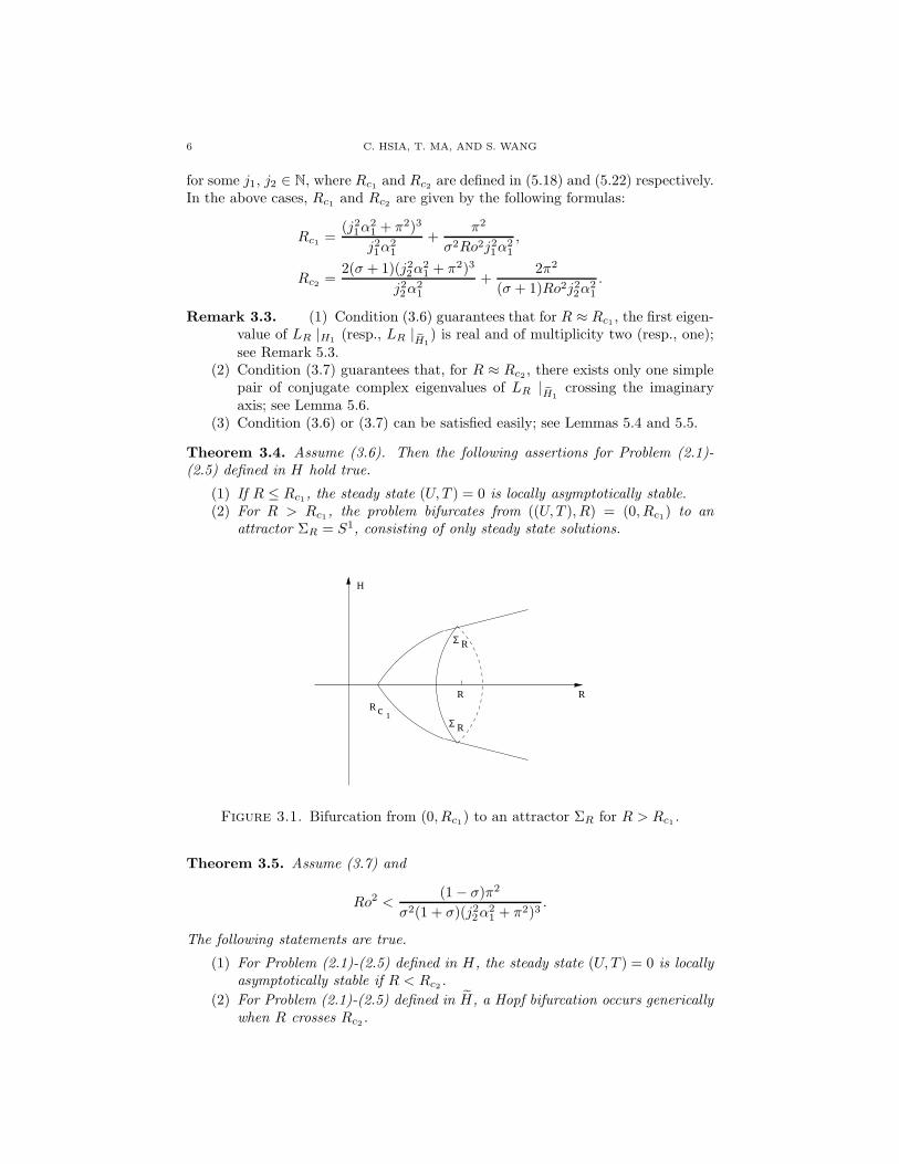
Theorem 3.4. Assume (3.6). Then the following assertions for Problem (2.1)-(2.5) defined in H hold true.

(1) If R ≤ Rc1 , the steady state (U, T ) = 0 is locally asymptotically stable.(2) For R > Rc1 , the problem bifurcates from ((U, T ), R) = (0, Rc1) to an

attractor ΣR = S1, consisting of only steady state solutions.

H

Σ

Σ

R

R

R

R

R c 1

Figure 3.1. Bifurcation from (0, Rc1) to an attractor ΣR for R > Rc1 .

Theorem 3.5. Assume (3.7) and

Ro2 <(1− σ)π2

σ2(1 + σ)(j22α21 + π2)3

.

The following statements are true.

(1) For Problem (2.1)-(2.5) defined in H, the steady state (U, T ) = 0 is locallyasymptotically stable if R < Rc2 .

(2) For Problem (2.1)-(2.5) defined in H, a Hopf bifurcation occurs genericallywhen R crosses Rc2 .


4. Preliminaries

4.1. Attractor bifurcation theory. Consider (3.1) satisfying (3.2) and (3.3).We start with the Principle of Exchange of Stabilities (PES). Let the eigenvalues(counting the multiplicity) of Lλ be given by β1(λ), β2(λ), · · · . Suppose that

(4.1) Reβi(λ)

< 0 if λ < λ0,

= 0 if λ = λ0,

> 0 if λ > λ0,

if 1 ≤ i ≤ m,

(4.2) Reβj(λ0) < 0, if m+ 1 ≤ j.

Let the eigenspace of Lλ at λ0 be

E0 =⋃

1≤j≤m

∞⋃

k=1

u, v ∈ H1 | (Lλ0 − βj(λ0))kw = 0, w = u+ iv.

It is known that dimE0 = m.

Theorem 4.1 (T. Ma and S. Wang [16, 17]). Assume that the conditions (3.2)-(3.5) and (4.1)-(4.2) hold true, and u = 0 is locally asymptotically stable for (3.1)at λ = λ0. Then the following assertions hold true.

(1) For λ > λ0, (3.1) bifurcates from (u, λ) = (0, λ0) to attractors Σλ, havingthe same homology as Sm−1, with m− 1 ≤ dimΣλ ≤ m, which is connectedif m > 1;

(2) For any uλ ∈ Σλ, uλ can be expressed as

uλ = vλ + o(‖vλ‖H1), vλ ∈ E0;

(3) There is an open set U ⊂ H with 0 ∈ U such that the attractor Σλ bifurcatedfrom (0, λ0) attracts U\Γ in H, where Γ is the stable manifold of u = 0 withco-dimension m.

4.2. Center manifold theory. A crucial ingredient for the proof of the maintheorems using the above attractor bifurcation theorem is an approximation formulafor center manifold functions; see [16].

Let H1 and H be decomposed into

(4.3) H1 = Eλ1 ⊕ Eλ2 , H = Eλ1 ⊕ Eλ2 ,

for λ near λ0 ∈ R1, where Eλ1 , Eλ2 are invariant subspaces of Lλ, such that dimEλ1 <

∞, Eλ1 = Eλ1 , Eλ2 = closure of Eλ2 in H . In addition, Lλ can be decomposed into

Lλ = Lλ1 ⊕ Lλ2 such that for any λ near λ0,

(4.4)

Lλ1 = Lλ|Eλ

1: Eλ1 −→ Eλ1 ,

Lλ2 = Lλ|Eλ2: Eλ2 −→ Eλ2 ,

where all eigenvalues of Lλ2 possess negative real parts, and the eigenvalues of Lλ1possess nonnegative real parts at λ = λ0. Furthermore, with µ < 1 given by (3.3),let

Eλ2 (µ) = closure of Eλ2 in Hµ.

By the classical center manifold theorem (see among others [7, 26]), there existsa neighborhood of λ0 given by |λ−λ0| < δ for some δ > 0, a neighborhood Bλ ⊂ Eλ1of x = 0, and a C1 center manifold function Φ(·, λ) : Bλ → Eλ2 (θ), called the center


manifold function, depending continuously on λ. Then to investigate the dynamicbifurcation of (3.1) it suffices to consider the finite dimensional system as follows

(4.5)dx

dt= Lλ1x+ g1(x,Φλ(x), λ), x ∈ Bλ ⊂ Eλ1 .

Hence, an approximation formula for the center manifold function Φλ is crucial forthe bifurcation and stability study.

Let the nonlinear operator G be in the following form

(4.6) G(u, λ) = Gn(u, λ) + o(‖u‖n),

for some integer n ≥ 2. Here Gn : H1 × · · · ×H1 −→ H is a n-multilinear operator,and Gn(u, λ) = Gn(u, · · · , u, λ).

Theorem 4.2. [16] Under the conditions (4.3), (4.4) and (4.6), the center manifoldfunction Φ(x, λ) can be expressed as

(4.7) Φ(x, λ) = (−Lλ2 )−1P2Gn(x, λ) + o(‖x‖n) +O(|Reβ| ‖x‖n),

where Lλ2 is as in (4.4), P2 : H → E2 the canonical projection, x ∈ Eλ1 , andβ = (β1(λ), · · · , βm(λ)) the eigenvectors of Lλ1 .

5. Eigenvalue Problem

The eigenvalue problem of the linearized problem of (2.1)-(2.4) is given by

(5.1)

σ(∆U −∇p) + σRTe−1

Roe× U = βU,

∆T + w = βT,

divU = 0,

supplemented with (2.3) and (2.4). For ψ = (U, T ) satisfying (2.3) and (2.4), weexpand the field ψ in Fourier series

(5.2) ψ(x, y, z) =

∞∑

j,k=−∞

ψjk(z)ei(jα1x+kα2y).

Plugging (5.2) into (5.1), we obtain the following system of ordinary differentialequations

(5.3)

σ(Djkujk − ijα1pjk) +1

Rovjk = βujk,

σ(Djkvjk − ikα2pjk)−1

Roujk = βvjk,

Djkwjk − p′jk +RTjk = σ−1βwjk,

DjkTjk + wjk = βTjk,

ijα1ujk + ikα2vjk + w′jk = 0,

u′jk |z=0,1= v′jk |z=0,1= wjk |z=0,1= Tjk |z=0,1= 0,


for j, k ∈ Z, where ′ = d/dz, Djk = d2/dz2 − α2jk and α2

jk = j2α21 + k2α2

2. If

wjk 6= 0, (5.3) can be reduced to a single equation for wjk(z):

(Djk − β)(σDjk − β)2Djk(5.4)

+1

Ro2(Djk − β)(Djk + α2

jk) + σRα2jk(σDjk − β)wjk = 0,

wjk = w′′

jk = w(4)jk = w

(6)jk = 0 at z = 0, 1,(5.5)

for j, k ∈ Z. Thanks to (5.5), wjk can be expanded in a Fourier sine series

(5.6) wjk(z) =∞∑

l=1

wjkl sin lπz,

for (j, k) ∈ Z × Z. Substituting (5.6) into (5.4), we see that the eigenvalues β ofthe problem (5.1) satisfy the cubic equations

β3 + (2σ + 1)γ2jklβ2 + [(σ2 + 2σ)γ4jkl +

l2π2

Ro2γ2jkl− σR

α2jk

γ2jkl]β(5.7)

+ σ2γ6jkl − σ2Rα2jk +

l2π2

Ro2= 0,

for j, k ∈ Z and l ∈ N, where γ2jkl = α2jk + l2π2. In the following discussions, we let

(5.8)

gjkl(β) = (β + γ2jkl)[(β + σγ2jkl)2 + l2π2Ro−2γ−2

jkl],

hjkl(β) = σRα2jkγ

−2jkl(β + σγ2jkl),

fjkl(β) = gjkl(β) − hjkl(β),

and βjkl1(R), βjkl2(R) and βjkl3(R) be the zeros of fjkl with

Re(βjkl1) ≥ Re(βjkl2) ≥ Re(βjkl3).

5.1. Eigenvectors. In the following discussions, we consider the following indexsets:

Λ1 = (j, k, l) ∈ Z2 × N | j ≥ 0, (j, k) 6= (0, 0),

Λ2 = (j, k, l) ∈ Z2 × 0 | j ≥ 0, (j, k) 6= (0, 0),

Λ3 = (j, k, l) ∈ (0, 0) × N,

Λ = Λ1 ∪ Λ2 ∪ Λ3.

1. For (j, k, 0) ∈ Λ2, we define

ψβjk0

1 = (kα2 sin(jα1x+ kα2y),−jα1 sin(jα1x+ kα2y), 0, 0)t,

ψβjk0

2 = (−kα2 cos(jα1x+ kα2y), jα1 cos(jα1x+ kα2y), 0, 0)t,

Ejk0 = spanψβjk0

1 , ψβjk0

2 ,

βΛ2 = ∪(j,k,0)∈Λ2βjk0,

where βjk0 = −σγ2jk0 = −σα2jk = −σ(j2α2

1 + k2α22). It is not hard to see that

LR(ψβjk0

1 ) = βjk0ψβjk0

1 and LR(ψβjk0

2 ) = βjk0ψβjk0

2 .


2. For (0, 0, l) ∈ Λ3, we define

ψβ00l1 = (0, 0, 0, sin lπz)t, ψβ0012 = (cos lπz, 0, 0, 0)t,

ψβ00l3 = (0, cos lπz, 0, 0)t, E00l = spanψβ00l1 , ψβ00l2 , ψβ00l3,

βΛ3 = ∪∞l=1 ∪

3q=1 β00lq, βeΛ3

= ∪∞l=1β00l1,

where β00l1 = −γ200l = −l2π2, β0012 = −σγ200l −1Ro i and β00l3 = −σγ200l +

1Ro i. It

is easy to check that

LR(ψβ00l1) = β0011ψ

β00l1 ,

LR(ψβ00l2) = −σγ200lψ

β00l2 −1

Roψβ00l3 ,

LR(ψβ00l3) =

1

Roψβ00l2 − σγ200lψ

β00l3 .

3. For (j, k, l) ∈ Λ1, we define

φ1jkl = (−jα1lπ

α2jk

sin(jα1x+ kα2y) cos lπz,−kα2lπ

α2jk

sin(jα1x+ kα2y) cos lπz,

cos(jα1x+ kα2y) sin lπz, 0)t,

φ2jkl = (kα2lπ

α2jk

sin(jα1x+ kα2y) cos lπz,−jα1lπ

α2jk

sin(jα1x+ kα2y) cos lπz, 0, 0),

φ3jkl = (0, 0, 0, cos(jα1x+ kα2y) sin lπz)t,

φ4jkl = (jα1lπ

α2jk

cos(jα1x+ kα2y) cos lπz,kα2lπ

α2jk

cos(jα1x+ kα2y) cos lπz,

sin(jα1x+ kα2y) sin lπz, 0)t,

φ5jkl = (−kα2lπ

α2jk

cos(jα1x+ kα2y) cos lπz,jα1lπ

α2jk

cos(jα1x+ kα2y) cos lπz, 0, 0)t,

φ6jkl = (0, 0, 0, sin(jα1x+ kα2y) sin lπz)t,

E1jkl = spanφ1jkl, φ

2jkl , φ

3jkl, E2

jkl = spanφ4jkl, φ5jkl, φ

6jkl,

Ejkl = E1jkl ⊕ E2

jkl, βΛ1 = ∪(j,k,l)∈Λ1∪3q=1 βjklq.

It is easy to check that E1jkl and E2

jkl are invariant subspaces of the linear op-

erator LR respectively, i.e., LR(E1jkl) ⊂ E1

jkl and LR(E2jkl) ⊂ E2

jkl . The char-

acteristic polynomial of LR |E1jkl

(resp., LR |E2jkl

) is given by fjkl as defined in

(5.8). Since E1jkl (resp.,E

2jkl) is of dimension three, the (generalized) eigenvectors

of LR |E1jkl

, ∪3q=1ψ

βjklq

1 (∪3q=1ψ

βjklq

2 ), form a basis of E1jkl (resp., E

2jkl), i.e.,

span∪3q=1ψ

βjklq

1 = E1jkl (resp., span∪

3q=1ψ

βjklq

2 = E2jkl). If βjklq is a real

zero of fjkl, the eigenvector corresponding to βjklq in E1jkl (resp., E2

jkl) is given by

ψβjklq

1 = φ1jkl +A1(βjklq)φ2jkl +A2(βjklq)φ

3jkl ,(5.9)

(ψβjklq

2 = φ4jkl +A1(βjklq)φ5jkl +A2(βjklq)φ

6jkl),

where

(5.10) A1(β) =−1

Ro(β + σγ2jkl), A2(β) =

1

β + γ2jkl.


If βjklq1 = βjklq2 (imaginary numbers) are zeros of fjkl, the (generalized) eigenvec-tors corresponding to βjklq1 and βjklq2 in E1

jkl (resp., E2jkl) are given by

(5.11)ψβjklq11 = φ1jkl +R1(βjklq1 )φ

2jkl +R2(βjklq1 )φ

3jkl,

ψβjklq21 = I1(βjklq1 )φ

2jkl + I2(βjklq1 )φ

3jkl,

ψ

βjklq12 = φ4jkl +R1(βjklq1 )φ

5jkl +R2(βjklq1 )φ

6jkl ,

ψβjklq22 = I1(βjklq1 )φ

5jkl + I2(βjklq1 )φ

6jkl ,

,

where

(5.12)R1(β) = Re(A1(β)), R2(β) = Re(A2(β)),

I1(β) = Im(A1(β)), I2(β) = Im(A2(β)).

The dual vector corresponding to ψβjklq

1 (resp., ψβjklq

2 ) is given by

Ψβjklq

1 = φ1jkl + C1(βjklq)φ2jkl + C2(βjklq)φ

3jkl ,(5.13)

(Ψβjklq

2 = φ4jkl + C1(βjklq)φ5jkl + C2(βjklq)φ

6jkl),

where

(5.14) C1(β) =1

Ro(β + σγ2jkl), C2(β) =

σR

β + γ2jkl.

The dual vector Ψβjklq

1 (resp., Ψβjklq

2 ) satisfies

< ψβjklq∗

1 ,Ψβjklq

1 >H= 0 (< ψβjklq∗

2 ,Ψβjklq

2 >H= 0),(5.15)

for q∗ 6= q.

We note that Ej1k1l1 is orthogonal to Ej2k2l2 for (j1, k1, l1) 6= (j2, k2, l2) and E1jkl

is orthogonal to E2jkl for (j, k, l) ∈ Λ1. Hence the dual vector Ψ

βjklq

1 (resp., Ψβjklq

2 )satisfies

< ψ,Ψβjklq

1 >H= 0 for ψ ∈ (∪(j∗,k∗,l∗) 6=(j,k,l)Ej∗k∗l∗) ∪E2jkl(5.16)

(< ψ,Ψβjklq

2 >H= 0 for ψ ∈ (∪(j∗,k∗,l∗) 6=(j,k,l)Ej∗k∗l∗) ∪ E1jkl).

In view of the Fourier expansion, we see that ∪(j,k,l)∈ΛEjkl is a basis of H1 and

(∪(j,k,l)∈Λ1E1jkl)∪(∪(j,k,0)∈Λ2

ψβjk0

1 )∪(∪(0,0,l)∈Λ3ψβ00l1) is a basis of H1. Hence,

by the discussion above, we have the following conclusions.

a) The set βH1 = βΛ1 ∪ βΛ2 ∪ βΛ3 consists of all eigenvalues of LR |H1 , and the(generalized) eigenvectors of LR |H1 form a basis of H1.

b) The set β eH1= βΛ1 ∪ βΛ2 ∪ βeΛ3

consists of all eigenvalues of LR | eH1, and the

(generalized) eigenvectors of LR | eH1form a basis of H1.

c) Re(β) < 0 for each β ∈ βΛ2 ∪ βΛ3 .

Lemma 5.1. If R is small, then Re(βjklq(R)) < 0 for each βjklq ∈ βΛ1 .


Proof. Plugging β = γ2jklβ∗ into fjkl, we get fjkl(β) = γ6jklfjkl(β

∗), where

fjkl(β∗) = (β∗ + 1)(β∗ + σ)2 +

l2π2

γ6jklRo2(β∗ + 1)− σR

α2jk

γ6jkl(β∗ + σ).

Hence, we only need to show that the real part of each zero of fjkl is strictly negative

when R is small. We observe that fjkl(β∗) > 0 for all β∗ ≥ 0 provided R < 1+σ−1.

Therefore, if all zeros of fjkl are real numbers, we are done.

For the case where only one of the zeros of fjkl is real, this real zero, β∗1 , is a

perturbation of −1. There exists an ǫ ( depending on σ only) such that −(1+2σ) <

β∗1 < 0 provided R < ǫ. This makes the real part of the other two zeros of fjkl

strictly negative and the proof is complete.

5.2. Characterization of Critical Rayleigh Numbers. Based on the abovediscussion, we know that only the eigenvalues in βΛ1 depend on the Rayleigh numberR. Hence, to study the Principle of Exchange of Stabilities for problem (5.1), itsuffices to focus the problem on the set βΛ1 . We proceed with the following twocases.

Case 1. β = 0 is a zero of fjkl if and only if the constant term of the polynomialfjkl is 0. In this case, we have

(5.17) R =γ6jklα2jk

+l2π2

σ2Ro2α2jk

≥(α2jk + π2)3

α2jk

+π2

σ2Ro2α2jk

.

Hence the critical Rayleigh number Rc1 is given by

(5.18) Rc1 = min(j,k,l)∈Λ1

γ6jklα2jk

+l2π2

σ2Ro2α2jk

=γ6j1k11α2j1k1

+π2

σ2Ro2α2j1k1

,

for some (j1, k1, 1) ∈ Λ1.Case 2. A careful analysis on (5.7) shows that β = ai (a 6= 0), a purely

imaginary number, is a zero of fjkl if and only if the following two equations holdtrue:

(σ2 + 2σ)γ4jkl +l2π2

Ro2γ2jkl− σR

α2jk

γ2jkl> 0,

(2σ + 1)γ2jkl[(σ2 + 2σ)γ4jkl +

l2π2

Ro2γ2jkl− σR

α2jk

γ2jkl]

= σ2γ6jkl − σ2Rα2jk +

l2π2

Ro2.

In this case, we have

R =2(σ + 1)γ6jkl

α2jk

+2l2π2

(σ + 1)Ro2α2jk

,(5.19)

R <(σ + 2)γ6jkl

α2jk

+l2π2

σRo2α2jk

.(5.20)

Plugging (5.20) into (5.19), we derive an upper bound for Ro2,

(5.21) Ro2 <(1− σ)l2π2

σ2(1 + σ)γ6jkl,


which could only hold true when σ < 1.As in Case 1, the minimum of the right hand side of (5.19) is always obtain at

l = 1. Hence the critical Rayleigh number Rc2 is given by

Rc2 = min(j,k,l)∈Λ1

2(σ + 1)γ6jkl

α2jk

+2l2π2

(σ + 1)Ro2α2jk

(5.22)

=2(σ + 1)γ6j2k21

α2j2k2

+2π2

(σ + 1)Ro2α2j2k2

,

for some (j2, k2, 1) ∈ Λ1. In the case of σ < 1, (5.21) with l = 1 implies Rc2 issmaller than Rc1 . Hence, for Problem (2.1)-(2.5), Rc1 is the first critical Rayleighnumber if σ > 1 and Rc2 is the first critical Rayleigh number if σ < 1. Therefore,the Principle of Exchange of Stabilities is given by Lemma 5.2 and Lemma 5.6.

Lemma 5.2. For fixed σ > 1 and Ro > 0, suppose that (α2jk, l) = (α2

j1k1, 1)

minimizes the right hand side of (5.17), then

(5.23) βj1k111(R)

< 0 if R < Rc1= 0 if R = Rc1> 0 if R > Rc1

,

(5.24) Reβjklq(R) < 0 for (α2jk , l) 6= (α2

j1k1 , 1), q = 1, 2, 3, R near Rc1 .

Proof. By the above discussion, we only need to show that the first eigenvaluecrosses the imaginary axis. We note that fj1k11(β) = 0 is equivalent to gj1k11(β) =hj1k11(β), i.e.,

(5.25) (β+γ2j1k11)[(β+σγ2j1k11)

2+ l2π2Ro−2γ−2j1k11

] = σRα2j1k1γ

−2j1k11

(β+σγ2j1k11).

We see that both gj1k11 and hj1k11 are strictly increasing for β > −γ2j1k11 ( since

σ > 1 ). Let Γ1 be the graph of η = gj1k11(β) and Γ2 be the graph of η = hj1k11(β)as shown in Figure 5.1. When R = Rc1 , Point S0, the intersecting point of Γ1 andΓ2 corresponding to βj1k11(R) ( i.e., the β coordinate of S0 is βj1k11(R)), is on the ηaxis. When R increases (resp., decreases), S0 becomes S1 ( resp., S2). This proves(5.23) and the proof is complete.


R<R

R=R

R>RC

C

C

1

1

1

β

S0

S

γj k 11 1

2

γσ j k 11 12

η

S

2

1

Γ

Γ2

1

Figure 5.1.

Remark 5.3. (1) In the proof of Lemma 5.2, as shown by (5.25) and Fig-ure 5.1, we see that, for R ≈ Rc1 , the first eigenvalue βj1k111 is a simplezero of fj1k11(β). We have seen in Section 5.1 that there are eigenvectors

ψβj1k111

1 ∈ E1j1k1l

and ψβj1k111

2 ∈ E2j1k1l

corresponding to βj1k111. Therefore,

the multiplicity of the first eigenvalue of L |H1 (resp., L | eH1) is mH1 = 2m

(resp., m eH1= m ), where m is the number of (j, k, 1)’s (∈ Λ1) satisfying

α2jk = α2

j1k1. Hence, Condition (3.6) guarantees that, for R ≈ Rc1 , the first

eigenvalue of LR |H1 (resp., LR | eH1) is real and of multiplicity two (resp.,

one).(2) For the classical Benard problem without rotation, the second term on the

right hand side of (5.17), hence the second term on the right hand side of(5.18), is not presented. Therefore, the first critical Rayleigh number of theclassical Benard problem depends only on the aspect of ratio; while the firstcritical Rayleigh number of the rotating problem depends on the aspect ofratio, the Prandtl number and the Rossby number. And it is clear thatthe first critical Rayleigh number of fast rotating flows is remarkably largerthan the first critical Rayleigh number of the classical Benard problem.This indicates that the rotating flows are much more stable than the non-rotating flows.

(3) Rc1 is the first Critical Rayleigh number if the Prandtl number is greaterthan one. For the case where the Prandtl number is smaller than one, Rc2is the first Critical Rayleigh number and, in general, there are a few criticalvalues between Rc2 and Rc1 .

For x > 0, b ≥ 0, we define

(5.26) fb(x) =(x+ π2)3 + b

x.

Let x = α2jk, then the right hand side of (5.18) could be expressed as fb1(x), where

b1 = π2

σ2Ro2 ; and the second line of (5.22) could be expressed as 2(σ + 1)fb2(x),


where b2 = π2

(σ+1)2Ro2 . Consider

(5.27) f′

b(x) =(2x− π2)(x + π2)2 − b

x2.

As shown in Figure 5.2, it is easy to see that

a) for x ∈ (0,∞), fb(x) has only one critical number xb,

b) f′

b(x) < 0 if x < xb,

c) f′

b(x) > 0 if x > xb,d) fb(xb) is the global minimum of fb(x), and

e) xb is strictly increasing in b , hence, xb1 > xb2 >π2

2 .

x

y

y = b

π 2

x b

2π 2

2π π 2 2y = (2x − )(x+ )

Figure 5.2.

In Lemmas 5.4 and 5.5, we consider the following different conditions

xb1 ≤ α21 < α2

2,(5.28)

α21 ≤

1

5xb1 < 2xb1 < α2

2,(5.29)

xb2 ≤ α21 < α2

2,(5.30)

α21 ≤

1

5xb2 < 2xb2 < α2

2.(5.31)

Lemma 5.4. (1) Condition (3.6) holds true under the assumption (5.28).(2) Generically, Condition (3.6) holds true under the assumption (5.29).

Proof. (1) Under the assumption (5.28), by c), we conclude that Rc1 is onlyobtained at (j, k, l) = (1, 0, 1), i.e. j1 = 1.

(2) Under the assumption (5.29), there exists j∗ ≥ 2 such that j∗2α21 ≤ xb1 <

(j∗ + 1)2α21. We note that

(j∗ + 1)2α21

< 2j∗2α2

1 < 2xb1 < α22 if j∗ ≥ 3,

= 9α21 <

95xb1 < 2xb1 < α2

2 if j∗ = 2.


Hence, by b) and c), we conclude that

Rc1 = minfb1(j∗2α2

1), fb1((j∗ + 1)2α2

1),

i.e., j1 = j∗ or j1 = j∗ + 1. Note that, by b) and c), generically fb1(j∗2α2

1) 6=fb1((j

∗ + 1)2α21). The proof is complete.

Lemma 5.5. (1) Condition (3.7) holds true under the assumption (5.30).(2) Generically, Condition (3.7) holds true under the assumption (5.31).

Proof. Consider

Rc2 = min(j,k,1)∈Λ1

2(σ + 1)fb2(α2jk).

The rest part of the proof is the same as the proof of Lemma 5.4.

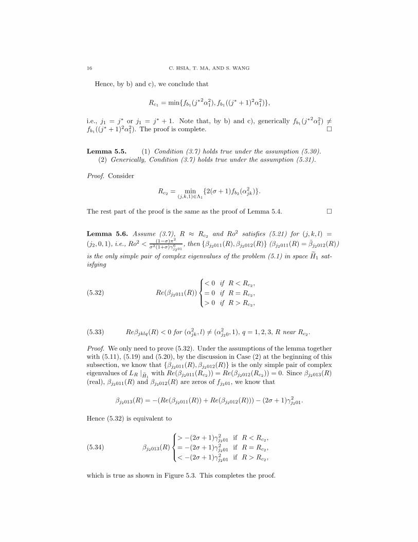
Lemma 5.6. Assume (3.7), R ≈ Rc2 and Ro2 satisfies (5.21) for (j, k, l) =

(j2, 0, 1), i.e., Ro2 < (1−σ)π2

σ2(1+σ)γ6j201

, then βj2011(R), βj2012(R) (βj2011(R) = βj2012(R))

is the only simple pair of complex eigenvalues of the problem (5.1) in space H1 sat-isfying

(5.32) Re(βj2011(R))

< 0 if R < Rc2 ,

= 0 if R = Rc2 ,

> 0 if R > Rc2 ,

(5.33) Reβjklq(R) < 0 for (α2jk, l) 6= (α2

j20, 1), q = 1, 2, 3, R near Rc2 .

Proof. We only need to prove (5.32). Under the assumptions of the lemma togetherwith (5.11), (5.19) and (5.20), by the discussion in Case (2) at the beginning of thissubsection, we know that βj2011(R), βj2012(R) is the only simple pair of complexeigenvalues of LR | eH1

with Re(βj2011(Rc2)) = Re(βj2012(Rc2)) = 0. Since βj2013(R)

(real), βj2011(R) and βj2012(R) are zeros of fj201, we know that

βj2013(R) = −(Re(βj2011(R)) +Re(βj2012(R)))− (2σ + 1)γ2j201.

Hence (5.32) is equivalent to

(5.34) βj2013(R)

> −(2σ + 1)γ2j201 if R < Rc2 ,

= −(2σ + 1)γ2j201 if R = Rc2 ,

< −(2σ + 1)γ2j201 if R > Rc2 ,

which is true as shown in Figure 5.3. This completes the proof.


Γ1

R > R

Γ2

R = R

R < RC2

C2

C2

η

β

( 2 σ + 1 ) γ 2

j 2

0 1−

− γ 2

j 2 0 1

− σ γ 2

j 2 0 1

Figure 5.3.

Lemma 5.7. For fixed α1, α2 > 0 and σ > 1, Rc1 → ∞ as Ro → 0. More

precisely, Rc1 = O(Ro−43 ).

Proof. Since b1 =π2

σ2Ro2 , by (5.27), xb1 = O(b131 ) as Ro→ 0. Hence,

Rc1 = O(fb1 (xb1)) = O(b231 ) = O(Ro−

43 ).

6. Proof of Main Theorems

6.1. Center manifold reduction. We are now in a position to reduce equationsof (2.1)-(2.5) to the center manifold. For any ψ = (U, T ) ∈ H1, we have

ψ =

∞∑

(j,k,l)∈Λ1

3∑

q=1

(xjklqψβjklq

1 + yjklqψβjklq

2 )

+∑

(j,k,0)∈Λ2

(xjk0ψβjk0

1 + yjk0ψβjk0

2 ) +

∞∑

l=1

3∑

q=1

x00lqψβ00lq .

Under the assumption (3.6), the first critical Rayleigh number is given by

(6.1) Rc1 =γ6j101α2j10

+π2

σ2Ro2α2j10

.

In this case, the multiplicity of the first eigenvalue is two and the reduced equationsof (2.1)-(2.5) are given by(6.2)

dxj1011dt

= βj1011(R)xj1011 +1

< ψβj1011

1 ,Ψβj1011

1 >H< G(ψ, ψ),Ψ

βj1011

1 ) >H ,

dyj1011dt

= βj1011(R)yj1011 +1

< ψβj1011

2 ,Ψβj1011

2 >H< G(ψ, ψ),Ψ

βj1011

2 ) >H .


Here for ψ1 = (U1, T1), ψ2 = (U2, T2) and ψ3 = (U3, T3),

G(ψ1, ψ2) = −(P (U1 · ∇)U2, (U1 · ∇)T2)t

and

< G(ψ1, ψ2), ψ3 >H= −

∫ 1

0

∫ 2π/α2

0

∫ 2π/α1

0

[< (U1 · ∇)U2, U3 >R3

+ (U1 · ∇)T2T3]dxdydz,

where P is the Leray projection to L2 fields. Let the center manifold function bedenoted by

(6.3) Φ =∑

β 6=βj1011

(Φβ1 (xj1011, yj1011)ψβ1 +Φβ2 (xj1011, yj1011)ψ

β2 ).

The direct calculation shows that

(6.4)

G(ψβj1011

1 , ψβj1011

1 ) = −(0,A1π

2

2j1α1sin 2j1α1x, 0,

A2π

2sin 2πz)t,

G(ψβj1011

1 , ψβj1011

2 ) = −(π2

2j1α1cos 2πz,

A1π2

2j1α1(cos 2πz − cos 2j1α1x), 0, 0)

t,

G(ψβj1011

2 , ψβj1011

1 ) = −(−π2

2j1α1cos 2πz,

−A1π2

2j1α1(cos 2j1α1x+ cos 2πz), 0, 0)t,

G(ψβj1011

2 , ψβj1011

2 ) = −(0,−A1π

2


A2π

2sin 2πz)t.

(6.5)

G(ψβj1011

1 ,Ψβj1011

1 ) = −(0,C1π

2


C2π

2sin 2πz)t,

G(ψβj1011

1 ,Ψβj1011

2 ) = −(π2

2j1α1cos 2πz,

C1π2

2j1α1(cos 2πz − cos 2j1α1x), 0, 0)

t,

G(ψβj1011

2 ,Ψβj1011

1 ) = −(−π2

2j1α1cos 2πz,

−C1π2

2j1α1(cos 2j1α1x+ cos 2πz), 0, 0)t,

G(ψβj1011

2 ,Ψβj1011

2 ) = −(0,−C1π

2


C2π

2sin 2πz)t,

where A1 = A1(βj1011), A2 = A2(βj1011) C1 = C1(βj1011) and C2 = C2(βj1011).Hereafter, we make the following convention:

o(2) = o(x2j1011 + y2j1011) +O(| βj1011(R) | ·(x2j1011 + y2j1011)),

o(3) = o((x2j1011 + y2j1011)3/2) +O(| βj1011(R) | ·(x

2j1011 + y2j1011)

3/2),

o(4) = o((x2j1011 + y2j1011)2) +O(| βj1011(R) | ·(x

2j1011 + y2j1011)

2).

By Theorem 4.2 and (6.4)-(6.5), we obtain

(6.6) Φ = Φβ(2j1)00

1 ψβ(2j1)00

1 +Φβ(2j1)00

2 ψβ(2j1)00

2 +Φβ0021

1 ψβ0021

1 + o(2),


where

Φβ(2j1)00

1 =A1π

2

σα4(2j1)0

(x2j1011 − y2j1011) + o(2), ψβ(2j1)00

1 = (0,−2j1α1 sin 2j1α1x, 0, 0)t,

Φβ(2j1)00

2 =A1π

2

σα4(2j1)0

(2x1011y1011) + o(2), ψβ(2j1)00

2 = (0, 2j1α1 cos 2α1x, 0, 0)t,

Φβ0021

1 =−A2

8π(x2j1011 + y2j1011) + o(2), ψβ0021

1 = (0, 0, 0, sin 2πz)t.

Note that for any ψi ∈ H1(i = 1, 2, 3),

< G(ψ1, ψ2), ψ2 >H= 0,(6.7)

< G(ψ1, ψ2), ψ3 >H= − < G(ψ1, ψ3), ψ2 >H ;(6.8)

and for any ψi ∈ Ejkl (i = 1, 2, 3),

(6.9) < G(ψ1, ψ2), ψ3 >H= 0.

The direct calculation shows that

(6.10) G(ψ, ψβj1011

i ) = 0 for ψ ∈ ψβ(2j1)00

1 , ψβ(2j1)00

2 , ψβ0021

1 , i = 1, 2.

Then by ψ = xj1011ψβj1011

1 + yj1011ψβj1011

2 +Φ(xj1011, yj1011) and (6.4)-(6.10), wederive that

< G(ψ, ψ),Ψβj1011

1 >H

= < G(ψβj1011

1 ,Φ),Ψβj1011

1 >H xj1011+ < G(ψβj1011

2 ,Φ),Ψβj1011

1 >H yj1011 + o(3),

=− < G(ψβj1011

1 ,Ψβj1011

1 ),Φ >H xj1011− < G(ψβj1011

2 ,Ψβj1011

1 ),Φ >H yj1011 + o(3),

=−2A1C1π

6

σα1α2σ4(2j1)0

(x2j1011 − y2j1011)xj1011 −A2C2π

2

8α1α2(x2j1011 + y2j1011)xj1011 + o(3),

−2A1C1π

6

σα1α2α4(2j1)0

(2xj1011yj1011)yj1011

=− (2A1C1π

6

σα1α2α4(2j1)0

+A2C2π

2

8α1α2)(x2j1011 + y2j1011)xj1011 + o(3).

Similarly, we obtain

< G(ψ, ψ),Ψβj1011

2 >H= −(2A1C1π

6

σα1α2α4(2j1)0

+A2C2π

2

8α1α2)(x2j1011 + y2j1011)yj1011 + o(3).

Hence, the reduction equations are given by

(6.11)

dxj1011dt

= βj1011(R)xj1011 + δ(x2j1011 + y2j1011)xj1011 + o(3),

dyj1011dt

= βj1011(R)yj1011 + δ(x2j1011 + y2j1011)yj1011 + o(3),

where

(6.12) δ = −(2A1C1π

4

σα4(2j1)0

+A2C2

8)/(

π2

j21α21

(1 +A1C1) + 1 +A2C2) < 0.

A standard energy estimate on (6.11) together with the center manifold theory showthat, for R ≤ Rc1 , (U, T ) = 0 is locally asymptotically stable for the problem (2.1)-(2.5). Hence by Theorem 4.1, the solutions to (2.1)-(2.5) bifurcate from (U, T,R) =


(0, Rc1) to an attractor ΣR. Moreover, by (6.11)-(6.12) together with Theorem 5.10in [18], we conclude that ΣR is homeomorphic to S1 in H .

6.2. Completion of the proof of Theorem 3.4. In this subsection, we provethat ΣR consists of steady state solutions. It is clear that the first eigenvalue ofLR| eH1

is simple for R ≈ Rc1 . By the Kransnoselski bifurcation theorem (see among

others Chow and Hale [4] and Nirenberg [21]), when R crosses Rc1 , the equations

bifurcate from the basic solution to a steady state solution in H . Therefore theattractor ΣR contains at least one steady state solution. Secondly, it’s easy tocheck that the equations (2.1)-(2.5) defined in H are translation invariant in thex-direction. Hence if ψ0(x, y, z) = (U(x, y, z), T (x, y, z)) is a steady state solution,then ψ0(x+ ρ, y, z) are steady state solutions as well. By the periodic condition inthe x-direction, the set

Sψ0 = ψ0(x+ ρ, y, z)|ρ ∈ R

is a cycle homeomorphic to S1 in H . Therefore the steady state of (2.1)-(2.5)generates a cycle of steady state solutions. Hence the bifurcated attractor ΣRconsists of steady state solutions. The proof of Theorem 3.4 is complete.

6.3. Proof of Theorem 3.5. The proof follows directly from the classical Hopfbifurcation theorem and Lemma 5.6.

References

[1] P. Cessi and G. R. Ierley, Symmetry-breaking multiple equilibria in quasi-geostrophic,

wind-driven flows, J. Phys. Oceanogr., 25 (1995), pp. 1196–1202.[2] J. Charney and J. DeVore, Multiple flow equilibria in the atmosphere and blocking, J.

Atmos. Sci., 36 (1979), pp. 1205–1216.[3] Z.-M. Chen, M. Ghil, E. Simonnet, and S. Wang, Hopf bifurcation in quasi-geostrophic

channel flow, SIAM J. Appl. Math., 64 (2003), pp. 343–368 (electronic).[4] S. N. Chow and J. K. Hale, Methods of bifurcation theory, vol. 251 of Grundlehren der

Mathematischen Wissenschaften [Fundamental Principles of Mathematical Science], Springer-Verlag, New York, 1982.

[5] H. A. Dijkstra, Nonlinear Physical Oceanography: A Dynamical Systems Approach to the

Large-Scale Ocean Circulation and El Nino, Kluwer Acad. Publishers, Dordrecht/ Norwell,Mass., 2000.

[6] M. Ghil and S. Childress, Topics in Geophysical Fluid Dynamics: Atmospheric Dynamics,

Dynamo Theory, and Climate Dynamics, Springer-Verlag, New York, 1987.[7] D. Henry, Geometric theory of semilinear parabolic equations, vol. 840 of Lecture Notes in

Mathematics, Springer-Verlag, Berlin, 1981.[8] G. Ierley and V. A. Sheremet, Multiple solutions and advection-dominated flows in the

wind-driven circulation. i: Slip, J. Marine Res., 53 (1995), pp. 703–737.[9] S. Jiang, F.-F. Jin, and M. Ghil, Multiple equilibria, periodic, and aperiodic solutions in a

wind-driven, double-gyre, shallow-water model, J. Phys. Oceanogr., 25 (1995), pp. 764–786.[10] F. F. Jin and M. Ghil, Intraseasonal oscillations in the extratropics: Hopf bifurcation and

topographic instabilities, J. Atmos. Sci., 47 (1990), pp. 3007–3022.[11] B. Legras and M. Ghil, Persistent anomalies, blocking and variations in atmospheric pre-

dictability, J. Atmos. Sci., 42 (1985), pp. 433–471.[12] J. L. Lions, R. Temam, and S. Wang, New formulations of the primitive equations of the

atmosphere and applications, Nonlinearity, 5 (1992), pp. 237–288.[13] , On the equations of large-scale ocean, Nonlinearity, 5 (1992), pp. 1007–1053.

[14] E. N. Lorenz, Deterministic nonperiodic flow, J. Atmos. Sci., 20 (1963), pp. 130–141.[15] , The mechanics of vacillation, J. Atmos. Sci., 20 (1963), pp. 448–464.[16] T. Ma and S. Wang, Bifurcation Theory and Applications, vol. 53 of World Scientific Series

on Nonlinear Science, Series A, World Scientific, 2005.


[17] , Dynamic bifurcation of nonlinear evolution equations and applications, Chinese An-nals of Mathematics, 26:2 (2005), pp. 185–206.

[18] , Geometric Theory of Incompressible Flows with Applications to Fluid Dynamics,vol. 119 of Mathematical Surveys and Monographs, American Mathematical Society, Provi-dence, RI, 2005.

[19] S. Meacham and P. Berloff, Instability of a steady, barotropic, wind driven circulation,J. Mar. Res., 55 (1997), pp. 885–913.

[20] , On the stability of the wind-driven circulation, J. Mar. Res., 56 (1998), pp. 937–993.[21] L. Nirenberg, Topics in nonlinear functional analysis, Courant Institute of Mathematical

Sciences New York University, New York, 1974. With a chapter by E. Zehnder, Notes by R.A. Artino, Lecture Notes, 1973–1974.

[22] J. Pedlosky, Resonant topographic waves in barotropic and baroclinic flows, J. Atmos. Sci.,38 (1981), pp. 2626–2641.

[23] , Geophysical Fluid Dynamics, 2nd Edition, Springer-Verlag, New-York, 1987.[24] S. Speich, H. Dijkstra, and M. Ghil, Successive bifurcations in a shallow-water model,

applied to the wind-driven ocean circulation, Nonlin. Proc. Geophys., 2 (1995), pp. 241–268.[25] H. Stommel, Thermohaline convection with two stable regimes of flow, Tellus, 13 (1961),

pp. 224–230.[26] R. Temam, Infinite-dimensional dynamical systems in mechanics and physics, vol. 68 of

Applied Mathematical Sciences, Springer-Verlag, New York, second ed., 1997.[27] G. Veronis, An analysis of wind-driven ocean circulation with a limited fourier components,

J. Atmos. Sci., 20 (1963), pp. 577–593.[28] , Wind-driven ocean circulation, part ii: Numerical solution of the nonlinear problem,

Deep-Sea Res., 13 (1966), pp. 31–55.

(CH) Department of Mathematics, Statistics, and Computer Science, The University

of Illinois at Chicago, Chicago, IL 60607

E-mail address: [email protected]

(TM) Department of Mathematics, Sichuan University, Chengdu, P. R. China

(SW) Department of Mathematics, Indiana University, Bloomington, IN 47405

E-mail address: [email protected]

STRATIFIED ROTATING BOUSSINESQ EQUATIONS …state bifurcation while Rc2 leads to the onset of the...

Documents

Transcript of STRATIFIED ROTATING BOUSSINESQ EQUATIONS …state bifurcation while Rc2 leads to the onset of the...