STRATEGIC ENTRY DECISIONS, ACCOUNTING SIGNALS, AND

RISK MANAGEMENT DISCLOSURE

by

Youli Zou

A thesis submitted in conformity with the requirements for the degree of Doctor of Philosophy

Joseph L. Rotman School of Management University of Toronto

July, 2013

© Copyright by Youli Zou (2013)

ii  

STRATEGIC ENTRY DECISIONS, ACCOUNTING SIGNALS, AND

RISK MANAGEMENT DISCLOSURE

Youli Zou

A thesis submitted in conformity with the requirements for the degree of Doctor of Philosophy

Joseph L. Rotman School of Management University of Toronto

ABSTRACT

This dissertation investigates the economic consequences from hedge accounting signals

and risk management disclosure. I first examine the product market consequences to these

accounting signals and related disclosure in Chapter 1, then stock market reactions to disclosure

requirements in Chapter 2.

Chapter 1 examines potential entrants’ strategic entry decisions in response to

incumbents’ accounting information and related disclosure. I predict that potential entrants are

more likely to enter markets in which the incumbents’ accounting information suggests higher

future production costs that are specific to the incumbents themselves. I further hypothesize that

the relation is stronger when the accounting signals are accompanied by more disclosure. Using

detailed U.S. airline industry data and hedge accounting disclosure under SFAS 133, I find that

potential entrants are more likely to enter routes in which the incumbents’ lower accumulated

other comprehensive income from fuel hedges suggests their higher future production costs. This

entry pattern is stronger when incumbents have more transparent annual report disclosure

regarding their fuel hedge programs. The entry pattern is also stronger after a systematic increase

in risk management disclosure requirements following the (exogenous) adoption of SFAS 161.

iii  

Chapter 2 analyzes stock returns of U.S. airlines around events leading up to the adoption

of SFAS 161. SFAS 161 enhanced the disclosure requirements for derivatives and hedging

activities. I find that U.S. airlines experienced statistically significant positive returns around the

key events leading up to the adoption of SFAS 161. I then examine the cross-sectional variation

of the returns around these events. Regression results provide initial support for the real effects

theory that greater disclosure requirements could distort firms’ hedging and production decisions

and lead to suboptimal behavior.

In summary, this dissertation provides evidence that competitors use hedge accounting

signals and related disclosure in making product market decisions. Meanwhile, additional risk-

management disclosures may also distort firms’ hedging and production behavior, leading to

suboptimal decisions. This dissertation sheds light on the ongoing projects by the FASB and the

IASB on hedge accounting and disclosure and informs the regulators that costs and benefits

should be weighted in hedge accounting policy setting.

iv  

ACKNOWLEDGMENTS

I would like to express my deepest appreciation to my supervisor, Ole-Kristian Hope, for his

continuous support, encouragement, and mentorship throughout my time at Rotman. I am also

grateful to the other members of my dissertation committee: Francesco Bova, Gus De Franco,

Scott Liao, and Giri Kanagaretnam (the external reviewer) for their excellent comments and

suggestions. I owe my special gratitude to Jeffrey Callen, Gordon Richardson, Franco Wong, Hai

Lu, Partha Mohanram, Baohua Xin, Aida Wahid, and other members of the Rotman community

for their help and support throughout. I dedicate this dissertation to my family: my husband and

best friend Yiwei, and my dearest parents.

v  

TABLE OF CONTENTS

ABSTRACT ii

ACKNOWLEDGMENTS iv

TABLE OF CONTENTS v

LIST OF TABLES viii

LIST OF APPENDICES ix

CHAPTER 1—STRATEGIC ENTRY DECISIONS, ACCOUNTING

SIGNALS, AND RISK MANAGEMENT DISCLOSURE 1

1.1 INTRODUCTION 1

1.2 LITERATURE REVIEW AND HYPOTHESES DEVELOPMENT 7

1.2.1 Literature Review: Competition and Disclosure 7

1.2.2 Institutional Background: The U.S. Airline Industry 11

1.2.3 Risk Management Accounting and Related Disclosures 15

1.2.4 Hypotheses Development 19

1.3 SAMPLE, VARIABLE MEASUREMENTS, AND RESEARCH

DESIGN 23

1.3.1 Sample Selection 23

1.3.2 Research Design 24

1.3.3 Measure of Entry Moves (ENTRY) 25

1.3.4 Measures of Incumbents’ AOCI from Fuel Hedge (I_AOCIFH),

Disclosure (I_DISC), and Firm Characteristics 26

1.3.5 Measures of Control Variables 27

1.3.6 Descriptive Statistics and Correlations 27

vi  

1.4 EMPIRICAL RESULTS 28

1.4.1 Main Results 28

1.4.2 Additional Analyses 31

1.4.2.1 Individual Disclosure Items 31

1.4.2.2 Potential Endogeneity of Disclosure 32

1.4.2.3 Product Market Consequences after Entry 34

1.4.2.4 Other Analyses 34

1.5 CONCLUDING REMARKS-- CHAPTER 1 37

CHAPTER 2: THE ECONOMIC IMPACT OF SFAS 161: EVIDENCE

FROM MARKET REACTIONS TO EVENTS SURROUNDING THE

PASSAGE OF THE STATEMENT IN THE U.S. AIRLINE INDUSTRY 39

2.1 INTRODUCTION 39

2.2 BACKGROUND 43

2.2.1 Hedge accounting, disclosure, and prior literature 43

2.2.2 History of events 46

2.3 HYPOTHESES DEVELOPMENT 48

2.3.1 Overall market reactions 48

2.3.2 Cross-sectional determinants of market reactions 49

2.4 RESEARCH DESIGN AND DATA 51

2.4.1 Research design 51

2.4.1.1 Stock price reactions 51

2.4.1.2 Cross-sectional analyses 52

2.4.2 Data and descriptive statistics 53

vii  

2.5 EMPIRICAL RESULTS 55

2.5.1 Mean stock price reactions 55

2.5.2 Results of cross-sectional analyses 57

2.5.3 Additional analyses and future research 59

2.6 CONCLUSIONS 60

REFERENCES 61

 

 

 

 

 

 

 

 

 

 

 

 

viii  

LIST OF TABLES Table 1: Variable Definitions—Chapter 1 78Table 2: Descriptive Statistics 80Table 3: Pearson Correlations 81Table 4: The Impact of Incumbents’ AOCIFH (I_AOCIFH) and its Interaction

with Disclosure on Entry: Probit Regressions Results 83

Table 5: Regressing Disclosure Scores on Year Indicators 85Table 6: The Impact of Incumbents’ AOCIFH (I_AOCIFH) on Entry: Pre- and

Post-SFAS 161 comparisons: Probit Regressions Results 86

Table 7: The Effects of Individual Disclosure Items on Entry: Probit Regressions Results

88

Table 8: 2SLS for Disclosure, Using I_FR as the Instrument Variable 91Table 9: Change in Ticket Fares before and after Entry, for Entry and Matched no

Entry Routes 93

Table 10: Entrant-Incumbent-Year Level Analyses: Dependent Variable=% of Entered Market Share

94

Table 11: Using Alternative Variable of Interest Measure: I_AOCIFH_ASIF 95

Table 12: The Impact of Incumbents’ AOCIFH (I_AOCIFH) on Entry: Partition by the Sign of I_AOCIFH and by the Direction of Fuel Price Change

97

Table 13: The Impact of Incumbents’ AOCIFH (I_AOCIFH) and its Interaction with Disclosure on Entry: Probit Regressions Using One-airport Present Carriers as Entrants

99

Table 14: Variables Definition—Chapter 2 101Table 15: Descriptive Statistics and Correlations (2005-2008 average) 102Table 16: Average Stock Returns around Event Dates during the Deliberation of

SFAS 161: U.S. Airline Industry 103

Table 17: Sefcik and Thompson (1986) Cross-sectional Analyses of Stock Price Reactions around Key Events: 1 Indicator

104

Table 18: Sefcik and Thompson (1986) Cross-sectional Analyses of Stock Price Reactions around Key Events: 7 Indicators

105

Table 19: Average Stock Returns around Event Dates during the Deliberation of SFAS 161: CRSP Sample

106

 

 

 

ix  

LIST OF APPENDICES

Appendix A: Construction of the Disclosure Score--Chapter 1 66

Appendix B: Description of the D.O.T. Databases and Review of the Airline Literature

67

Appendix C: Journal Entries related to Cash Flow Hedges 70

Appendix D: Summary of SFAS 133 Disclosure Requirements 72

Appendix E: Summary of Events 74

Appendix F: Construction of the Disclosure Score--Chapter 2 75

Appendix G: Summary of SFAS 161 disclosure requirements 76

 

1

CHAPTER 1—STRATEGIC ENTRY DECISIONS, ACCOUNTING SIGNALS, AND

RISK MANAGEMENT DISCLOSURE

1.1 Introduction

This paper directly investigates the product market consequences of firms’ accounting

signals and related disclosures. Firms are sophisticated users of information disclosed by their

peer firms. Before making major strategic product-market moves, firms collect decision-relevant

information. One major type of information collected is competitors’ accounting information

related to competitive advantages and disadvantages. In this paper, I show that incumbents’

accounting signals and disclosures related to their risk management activities are relevant to

potential entrants’ product market decisions.

There is limited prior evidence of the product market consequences to disclosure. The

reason is that the relation between competition and disclosure depends on both the nature of the

competition and the nature of the information (Darrough 1993; Verrecchia 1990) – two factors

which are challenging to capture empirically. The U.S. airline setting allows me to directly

examine the association between potential entrant decisions and firm-specific accounting signals.

Verrecchia (1990) discusses how the two types of settings— one where the competitor is a

potential entrant and the other where the competitor is an existing rival—can generate opposite

predictions on the relation between disclosure and competition. In the airline setting, each route

is considered a separate market where potential entrants and existing incumbents are easily

identified. Moreover, Darrough (1993) and Sankar (1995) note that the type of information also

matters when competitors make product market decisions. Being vulnerable to jet fuel price

fluctuations, airlines use fuel hedge derivatives extensively to manage and control their operation

2

costs. The usage of jet fuel hedges varies significantly across the industry, and a successful

hedge program serves as an effective cost control, thus providing potential competitive

advantages. The accounting and disclosure regulations for fuel risk management fall under the

provisions of Statement of Financial Accounting Standards No. 133 Accounting for Derivative

Instruments and Hedging Activities (SFAS 133), and its later amendment Statement of Financial

Accounting Standards No. 161 Disclosure about Derivative Instruments and Hedging Activities

(SFAS 161). These regulations provide potentially valuable firm-specific cost-related

information to financial information users, including competitors.

I first show that, after controlling for numerous other economic determinants of entry

decisions, potential entrants are more likely to enter markets in which the incumbents’ cash flow

hedge signals indicate poorer cost control and higher future fuel expenses. Potential entrants are

defined as airlines which operate at both airports of a route but are not operating the route per se,

consistent with prior literature that uses airport presence as entry threat proxies. Under SFAS 133,

the accumulated other comprehensive income from fuel hedges (AOCIFH) stores the unrealized

gains/losses from unsettled cash flow hedge derivatives, which will be reclassified into fuel

expenses (and net income) when the forecasted transactions take place in the future. I manually

collect the AOCIFH information from all airlines’ 10K filings. The accounting construct of

AOCIFH varies with the firm’s specific hedging strategies, and describes how much future costs

will be reduced or increased due to hedging activities. Given the common jet fuel spot prices all

airlines face, a higher AOCIFH can reduce future fuel expenses by a greater amount, make the

firm more competitive in pricing, and serve as a deterrent for potential entries. Similarly, a

negative AOCIFH will increase future fuel expenses and decrease net income, putting the firm at

3

competitive disadvantage. Thus, incumbents’ firm-specific cost information can play an

important role in potential entrants’ strategic decisions.1

I further examine how financial disclosure related to this firm-specific accounting signal

affects the relation between the probability of entry and AOCIFH. Specifically, I empirically test

whether the relation between incumbents’ fuel hedge signals and the probability of entry is

stronger when the incumbents’ disclosure about their hedge activities is more extensive. The

motivation to assess AOCIFH and disclosure jointly stems from concerns of the Financial

Accounting Standards Board (FASB) that investors may not fully understand the impact of cash

flow hedge accounting on future firm performance due to the complexity of the standard. As a

result, firms provide supplementary disclosures in their financial reports to help users interpret

such signals and boost their informativeness. By carefully reading through the annual reports of

my sample firms and referring to risk management disclosure regulations and extant literature, I

construct a disclosure score based on the items in 10-K filings that relate to risk management

activities. The scores suggest that there is significant variation in supplementary disclosure –

both over time and across firms. I find that the relation between cash flow hedge signals and

entry by potential entrants is stronger when the hedge accounting signals are accompanied with

more extensive disclosures.

Finally, in response to the complaint that hedge accounting treatments under SFAS 133

are complicated and related financial report disclosures still do not provide adequate information

to users, the FASB issued SFAS 161 effective in 2008 with expanded quantitative and qualitative

1 Many studies have examined entry deterrence strategies with incomplete information. For example, Milgrom and

Roberts (1982) present a model where the incumbent and the entrant only know their own production costs but can

infer each other’s cost structure through pricing. In equilibrium, the incumbent uses limited pricing to signal his low

cost and deter entry, because the entrant uses the product price to infer the incumbent’s cost and expected post-entry

profits. In practice, other firm-specific information can validate and complement the pricing signal, and play

important roles in the entry game.

4

disclosure requirements for hedge derivatives. This exogenous shock to the risk management

disclosure regime provides a pseudo natural experiment to test the impact of disclosure on the

relation between entry patterns and accounting signals. I find that after the overall information

environment for risk management activities was improved following the adoption of SFAS 161,

the relation between cash flow hedge signals and the entry pattern of potential entrants becomes

significantly stronger compared with the pre-SFAS 161 period.

To further explore the information content of the disclosure regarding hedging activities,

I examine how individual disclosure items affect the informativeness of hedging signals

differently. My results suggest that three disclosure items—estimated reclassification into net

income in the next year, maturity of the derivatives, and separate disclosure of AOCIFH—are

considered the most helpful by potential entrants.

My results are robust to a battery of additional tests. To mitigate the potential

endogeneity issue with disclosure, I employ an instrumental variable approach. In addition, I

include carriers present at only one airport as potential entrants and rerun the tests. I also conduct

several other robustness tests, including controlling for additional known determinants of

disclosure, partitioning AOCIFH by its sign and rerunning the tests for both subsamples,

accounting for fuel hedges not designated as cash flow hedges, changing the scalar for the test

variable, and varying the sample size. Finally, when I collapse my sample to incumbent-entrant-

level and examine the entry pattern, the results are consistent with my primary results at route-

entrant-year level.

This study contributes to the growing literature on proprietary costs of disclosure (e.g.,

Verrecchia 1983, 1990; Darrough and Stoughton 1990; Darrough 1993; Bamber and Cheon 1998;

Guo, Lev, and Zhou 2004; Bhojraj, Blacconiere, and D’Souza 2004; Berger and Hann 2007; Li

5

2010; Bens, Berger, and Monahan 2011; Bova, Dou, and Hope 2012; Ellis, Fee, and Thomas

2012). The maintained assumption in this line of literature is that disclosure of certain

information compromises disclosing firms’ competitive advantages because such information

can be used strategically by competitors against disclosing firms. Analytical studies

unambiguously specify the type of information and the type of competition in order to generate a

directional prediction for the relation between disclosure and competition. By using a unique

setting in which I can clearly identify the nature of the information and the nature of the

competition, this paper provides for a more powerful setting to assess the product market

consequences of firm-specific signals and related disclosure. My findings support both the

proprietary cost of disclosure theory and the notion that product market consequences of

disclosure exist. This paper also suggests that further research on the determinants of disclosure

should consider both the nature of the competition and the nature of the information and choose

proxies accordingly.

Additionally, my findings enrich our understanding of SFAS 133 and related regulations.

Despite prescribing more uniform accounting treatments and disclosure rules for derivatives,

SFAS 133 has also been criticized for creating inconsistency and confusion, especially with the

cash flow hedge accounting treatment (e.g., Gigler, Kanodia, and Venugopalan 2007). Existing

research primarily focuses on the financial market implications of the standard (e.g., Campbell

2011; Ahmed, Kilie, and Lobo 2006; 2011) or the impact on firms’ risk management behavior

(Zhang 2009). By providing evidence that potential entrants use incumbents’ cash flow hedge

signals to facilitate their entry decisions, my results provide another channel through which the

information content of hedge accounting treatments and disclosure can be evaluated.

6

This article is also one of the first to empirically investigate the effectiveness of SFAS

161. The purpose of SFAS 161 was to provide financial statement users with enhanced

quantitative and qualitative disclosure for hedging activities. My paper provides evidence that

hedge accounting signals proposed by SFAS 133 become more informative in assisting potential

entrants’ strategic decisions after the adoption of SFAS 161 in the U.S. airline industry. This

result is consistent with the purpose of SFAS 161 in helping financial report users better

understand firms’ risk management activities and their impact on future performance.

In examining the effectiveness and informativeness of SFAS 133 and SFAS 161, this

study proposes an alternative approach to evaluating the information content of accounting

numbers and disclosures. Firms operating in the same product market are familiar with the

business practices within the industry and are sophisticated users of peer firms’ information.

Thus, their evaluation of the information content of accounting measures and disclosure

complements the traditional capital market value relevance approach.

Finally, my research extends the industrial organization literature that examines how

firms learn from their rivals in order to optimize decisions. Accounting information, which

represents firms’ essential operating and financing results, is largely ignored in the industrial

organization literature. Studies explaining the competition process and pattern tend to select

market-level structure and characteristic variables as major candidates (Oliveria 2008;

Boguslaski, Ito, and Lee 2004). This paper demonstrates the important role of competitors’ firm-

specific accounting information in the strategic entry process.

The next section provides a review of relevant literature and develops the hypotheses.

Section 1.3 describes the research design and sample selection. Section 1.4 presents empirical

7

results and Section 1.5 concludes the paper and Appendix A explains the disclosure score

construction and provides descriptive statistics for the disclosure items.

1.2 Literature Review and Hypotheses Development

1.2.1 Literature Review: Competition and Disclosure

Financial disclosure provides information to facilitate internal and external users’

decision making process. While shareholders use accounting information to allocate capital and

evaluate managers, firms collect their competitors’ information and choose their own

information sharing strategies to optimize their product market decisions (e.g., Gal-Or 1985,

1986; Vives 1984, 1990; Milgrom and Roberts 1982). Thus, competitors’ use of information

provides another benchmark against which the information content of accounting signals and

disclosures can be evaluated. While existing accounting research mainly focuses on financial

market implications of accounting measures and related disclosure (see Beyer, Cohen, Lys, and

Walther 2010 for a comprehensive survey), the use of such information by other external parties

is relatively unexplored empirically. This paper aims to fill this gap by examining how potential

entrants respond to incumbents’ firm-specific accounting signals, and how additional disclosure

regarding the signals impacts the response of potential entrants.

Using competing firms’ product market decisions as an information content criterion

requires clear identification of the nature of the information and the nature of the competition.

For instance, revealing information to competitors does not necessarily reduce the disclosing

firm’s competitive advantages. In some cases, firms are better off sharing information so as to

coordinate actions to their mutual advantages. Thus, the consequences of disclosure depend on

the specific type of competition firms are engaged in and the type of information firms have.

8

For this reason, analytical studies are particular specific in the type of competition and

the type of information in developing their models. Gal-Or (1986) and Vives (1984) examine the

information sharing strategies in an oligopoly and find that the disclosure decisions and the

optimality of segment or aggregate reporting depend on the type of competition and the nature of

the uncertainty in the economy. Feltham, Gigler, and Hughes (1992) consider the consequences

of line-of-business versus aggregate reporting in an entry game and show that incumbents may

distort their first-period production in an attempt to influence entrant beliefs because line-of-

business reporting provides entrants with proprietary information about the incumbent. Darrough

(1993) analyzes both ex ante and ex post disclosure incentives with market-wide demand and

firm-specific cost information in both Cournot and Bertrand settings. She finds that, ex ante,

firms would not commit to disclosure in Bertrand/cost and Cournot/demand cases. She further

demonstrates that firms’ incentives diverge ex post. Specifically, in equilibrium, disclosure

would seldom be observed when products are highly substitutable in the Bertrand/cost case.

However, in the Cournot/demand case, virtually all values of private information would be

disclosed. There are other studies examining the ex post disclosure incentives. Sankar (1995)

compares firm-specific and industry-wide information sharing in a Cournot duopoly setting. Her

results indicate that ex post, unfavorable news is disclosed and favorable news is withheld if the

signal is more informative about an industry-wide shock. In contrast, favorable news is disclosed

and unfavorable news is withheld if the signal is more informative about firm-specific shocks.

Darrough and Stoughton (1990) investigate the disclosure of market-level information in an

entry-game setting and posit that bad market-level news can serve as entry deterrence. These

differing predictions on the relation between disclosure and competition are rooted on the

premises that different types of information produce distinct product market consequences.

9

Accompanying the development of theoretical studies on competition and disclosure,

empirical researchers try to test such theories in different settings. Harris (1998) investigates the

relation between managers’ choices of which operations to report as business segments and

levels of industry competition using industry concentration ratios and abnormal profit adjusting

rates as the proxies. She finds that operations in less competitive industries are less likely to be

reported as industry segments, suggesting that the competitive harm cited as a disincentive to

segment reporting arises from a desire to protect abnormal profits and market shares in less

competitive markets. Using a Census Bureau database of confidential, plant-level data, Bens et al.

(2011) find similar results that a pseudo-segment is more likely to be aggregated when the

proprietary costs of separate reporting are high.2

Bamber and Cheon (1998) focus on managers’ decisions about how and where to

disclose earnings forecasts and examine how these decisions relate to proprietary costs proxied

by growth opportunity and industry concentration ratios. They find that forecasts made by firms

experiencing high growth opportunities or in concentrated product-markets are likely to be more

reactive and reluctant disclosures issued to limited audiences. Li (2010) looks at how

management forecasts quantity and quality are affected by product market competition and finds

that competition from potential entrants (captured by industry plant and equipment size)

increases disclosure quantity while competition from existing rivals (captured by industry

concentration ratio) decreases disclosure quantity, and that the association is less pronounced for

industry leaders.

2 Less competitive (high concentration ratios) does not necessary mean low proprietary cost. Instead, in Harris

(1998), a less competitive environment measured by a slower abnormal profit adjusting rate and a higher industry

concentration ratio means more to lose for the firm, thus higher proprietary costs. In many other settings (e.g.,

Verrecchia and Weber 2006; Li 2010), by more competitive (a lower concentration ratio), the authors mean higher

proprietary costs. This phenomenon further highlights the necessity of identifying the nature of competition.

10

Being aware that the traditional competition measures such as concentrations ratios and

industry profitability and size measures are crude and may not capture the competition nature

they intend to,3 more recent studies start to examine the disclosure behavior in particular

industries or settings and complement with competition proxies specific to these settings. Guo et

al. (2004) investigate the disclosure of product related information by Biotech firms in their IPOs

and their competition measures include the availability of a patent, stage of the product, and the

availability of venture capital. They find that these three proprietary cost proxies stand out as

consistent determinants of the extent of disclosure by IPOs. Bhojraj et al. (2004) focus on the

electric utility industry’s disclosure of strategies to protect the firm’s existing customers base and

plans to exploit emerging opportunities under deregulation and find that product market-related

incentives (greater threat of competitor entry captured by higher expected future market demand)

deter disclosure. Dedman and Lennox (2009) investigate the disclosure of sales and cost of sales.

In addition to using industry concentration ratios and abnormal profits as competition proxies,

they also employ a measure constructed from surveying managers about their perceived

competition. Ellis et al. (2012) choose the setting of disclosure about firms’ customers and use

the rate of nondisclosure of a firm’s rivals as one of their competition proxies. They find that an

individual firm’s decision to conceal information about its major customers is strongly associated

with the rate at which its rivals conceal information regarding their customers.

To summarize, this line of growing literature suggests that in order to have a clear and

directional prediction on the association between competition and disclosure, one has to specify

both the nature of the competition and the nature of the information. The U.S. airline industry

setting provides an ideal setting to identify and distinguish the nature of information and the

nature of competition.

3 See Karuna (2010) and Ali et al. (2009) for detailed discussion.

11

1.2.2 Institutional Background: The U.S. Airline Industry

The U.S. Airline Deregulation Act in 1978 gradually removed government control over

fares, routes, and market entries, and allowed free competition in the U.S. passenger air travel

market.4

Meanwhile, the industry is still under the supervision of the Department of

Transportation (D.O.T hereafter) and is required to provide substantial filings which are publicly

available (e.g., ticket prices, on-time performance, passenger volume, financial statements, etc.).5

With active competition and a rich data environment, a long line of literature has used the airline

industry to examine various competition-related research questions (Borenstein 1989; Berry

1990; Borenstein and Rose 1994; Hayes and Ross 1998; Boguskaski et al. 2004; Goolsbee and

Syverson 2008; Gerardi and Shapiro 2009; Aguirregabiria and Ho 2012, among many others).

I explore the U.S. airline setting to examine the informational role of accounting signals

and disclosure in potential entrants’ product market decisions. The airline industry setting offers

several advantages over cross-industry studies. First, each route is considered a unique product

market with the transportation service between the two airports provided by carriers being

homogenous or highly substitutable products.6 Defining markets and examining competition at

the route level is a common procedure in the economics literature on competition using the

airline industry setting. For example, Borenstein and Rose (1994) study the dispersion in prices

4 Extensive research has been conducted to determine whether the competition in the airline industry is closer to the

Bertrand or Cournot model. Brander and Zhang (1990) conclude that the competition in the airline industry is closer

to the Cournot type, but their conclusion stems from analysis of only non-stop flights on selected duopolistic

markets originating from the congested O’Hara airport. More recent studies find that the competition is closer to the

Bertrand type. Neven, Roller, and Zhang (1998) provide an industry-wide analysis of the European market and find

that the pattern is consistent with Bertrand competition. Busse (2002) examines the price war in the U.S airline

industry and discovers that over the time period the paper considers (1985-1992) price cuts by one airline were

always matched by competitors. The findings suggest that fierce price competition is characteristic in the

deregulated U.S airline industry. Besides, rather narrow observed profit margins in the industry are not consistent

with Cournot-type competition. 5 Please see the U.S. Department of Transportation websites (http://www.dot.gov and http://www.rita.dot.gov) for

data available for the airline industry. 6 Meanwhile, the supply, demand, and product prices for each product market are available through public

resources. For example, the D.O.T provides passenger volumes for each carrier-route, and the Origin and

Destination Survey (DB1B) database surveys 10% of all tickets quarterly, including ticket prices

12

airlines charge to different customers in the same product market, where the same product

market is defined as the same route. Using the U.S. airline setting, Goolsbee and Syverson (2008)

examine how incumbents respond to the threat of entry by competitors and define the

incumbents and the threat of entry at the route-quarter level. Gerardi and Shapiro (2009) analyze

the effects of competition on price dispersion in the airline industry using a panel data in which

an observation is a flight conducted by a specific airline between two airports in a specific time

period. Furthermore, Aguirregabiria and Ho (2012, 163) write the following: “Definition of a

market and a product. From the point of view of airlines’ entry and exit decisions, a market is a

non-directional city-pair. For the model of demand and price competition, a route is a directional

round-trip between an origin city and a destination city. These definitions are the same as

in Berry (1992) and Berry et al. (2006), among others, and similar to the ones used by Borenstein

(1989) or Ciliberto and Tamer (2009) with the only difference that they consider airport-pairs

instead of city-pairs.” Please see Appendix B for a complete discussion of the databases and

review of airline studies using the similar setting.

A well-defined product market is essential in addressing what the relation is between

competition and disclosure. The research design in this paper, where markets are defined as

routes, complements the traditional way of defining markets using SIC codes and measuring

competition with concentration ratios by two- or three-digit SIC codes. SIC code-based

competition proxies could also produce misleading results because they only include public firms

in the calculations. Ali, Klasa, and Yeung (2009) replicate prior studies and show that some of

the results reverse when both public and private firms are included in the competition proxy

calculation. Using each route as a market avoids such problems because the market share data for

all carriers are publicly available.

13

In addition, incumbents and potential entrants are directly observable for each route in the

airline industry. In particular, I am able to identify carriers who posit the most entry threats to

incumbents. Following prior economics research using airport presence as proxies for entry

threat (Hurdle et al. 1989; Sinclair 1995; Goolsbee and Syverson 2008), potential entrants are

defined as those carriers who operate at both of the airports but are not operating the route per se.

For example, an airline has flights to and from Boston, as well as flights to and from Cleveland,

but has not yet operated the Boston-Cleveland route per se. In this case, the airline posits the

most significant threat to the incumbent carriers of the route because it is already paying for slots

at both airports and the marginal cost of entering is relatively low. Goolsbee and Syverson (2008)

estimate that operating at both endpoints of a route translates into a 70 times higher probability

of entering for the route than for other routes. Consistent with this finding, most of the entries in

my sample period are launched by carriers operating at both airports.

The U.S. airline industry is characterized by fierce price competition.7 Demand is price-

sensitive and carriers have limited pricing power over consumers. Meanwhile, fuel and labor

costs are the two biggest cost drivers of the industry, exceeding 50% of total operating

expenses.8 Importantly, compared with labor (and other) costs, fuel prices are highly volatile and

uncertain, explaining 78.9% of the variation in total operating costs of my sample. The jet fuel

spot price in commodity markets is an external factor that airlines have little control over, and

fuel-price increases cannot be easily passed through to customers because of competitive

pressures. Airlines have tried repeatedly to raise fares in response to high fuel costs, but with

7 Forming airline alliances is another form of the competition dynamics in the industry. By joining an alliance,

airlines can (1) extend their network through code sharing; (2) reduce costs through sharing maintenance/operational

facilities. I exclude code sharing observations by eliminating tickets with ticketing carriers different from operating

carriers. The facilities/maintenance sharing usually happens between one legacy and one really small airline that

sole operate under the legacy airline or international airlines. These observations are immaterial in my sample. 8 According to U.S. Air Transport Association reports, for 2010 Q3, fuel and labor costs represent 25.4% and 24.7%

of operating expenses, respectively. For more summary data on U.S. air transportation, please see

http://www.airlines.org/Economics/DataAnalysis/Pages_Admin/DataAnalysis.aspx.

14

little success. For example, Continental Airlines rescinded a fare hike after trying a number of

times to boost overall fares. The airline said the airfare increases were due to high fuel costs, but

intense airline competition left the firm unable to pass along fuel costs to customers.9

In order to manage fuel price risk and achieve price competitiveness, airlines intensively

engage fuel hedges using jet-fuel related derivatives. Typical derivative instruments include

forward contracts, futures contracts, options, collars, swaps, etc. (Clubley 1999; Morrell and

Swan 2006). Fuel hedge contracts serve as a cost control mechanism for airlines. Chang and

Shao (2011) compare operating cost control strategies for airlines and rank fuel hedging

strategies as the second most significant and important among the 21 strategies extracted from

questionnaires answered by airline industry experts.

Despite the fact that all carriers face the same spot fuel price and that they all hedge their

fuel, the extent of hedging, the derivatives used, and the hedging outcomes vary significantly.10

Given the thin profit margin in the airline industry, the ability to manage market risk and reduce

fuel expenses is essential for future performance and is highly valued in the industry.11

Carter,

Rogers, and Simkins (2006a, 2006b) show that fuel hedge is positively related to firm value in

the U.S. airline industry (see also Allayannis and Weston 2001; Mackay and Moeller 2007;

Bartram, Brown, and Conrad 2011).12

Under the provisions of SFAS 133, airlines designate

these derivatives as cash flow hedges if they pass certain criteria. This accounting standard

intends to provide financial statement users with more transparent information on firms’ use of

9 See “Continental Raises Domestic Fares, Cites Fuel costs” (Reuters, February 27, 2004) and “Continental Airlines

Resends Latest Fare Hike” (Reuters, June 7, 2004). 10

Commenting on fuel hedge strategies in the industry, the Chief Financial Officer of United Airlines, Kathryn

Mikells, said in 2010 that “As an industry we are highly fragmented. Everybody has taken a different position.” See

http://www.reuters.com/article/2010/02/25/us-travel-leisure-summit-fuel-hedging-idUSTRE61O59Z20100225 11

Vice President of Southwest Airline Scott Topping highlighted that “fuel hedging will continue to play a strategic

role in the industry and be a potential source of competitive advantage” (Carter et al. 2006a). 12

Campello, Lin, Ma, and Zou (2011) identify several specific mechanisms through which hedging can affect real

and financial corporate outcomes. Another motivation implied in the literature for corporate hedging is to signal

management competence (DeMarzo and Duffie 1995; Morrell and Swan 2006).

15

derivative instruments. I discuss the accounting treatment and disclosure requirements for cash

flow hedge under SFAS 133 in more detail in the following section.

1.2.3 Risk Management Accounting and Related Disclosures

The last decades have witnessed impressive growth in the use of financial derivatives and

instruments in risk management. Before the adoption of SFAS 133 in 2000, the accounting

treatment for derivative instruments was incomplete and inconsistent.13

As a result, the FASB

has issued a series of accounting and disclosure requirements for derivatives, intending to supply

more publicly available information and improve the information content of derivatives.14

This

suggests that the FASB believes that such information is beneficial to financial statement users.

Following these regulations on enhanced disclosure, studies have emerged examining the

usefulness and value relevance of such disclosures (Venkatachalam 1996; Wong 1999; Seow and

Tam 2002; Jorion 2002). The general theme from this line of research is that expanded

disclosures provide incremental information to the market and are value-relevant.

To address the concern that historical-cost accounting and prior disclosure requirements

may not fully reflect a firm’s underlying risk profile, SFAS 133 requires that an entity must

recognize all derivatives in the balance sheet at fair values, and record changes in fair values of

the derivatives in corresponding accounts, depending on which kind of hedge the derivatives are

designated as. Three categories of hedges are allowed: hedges for foreign currency exposure,

fair-value hedges for recognized assets, and cash flow hedges for recognized assets or forecasted

13

Under the FASB Accounting Standards Codification effective for interim and annual periods ending after

September 15, 2009, SFAS 133 corresponds to ASC 815 and SFAS 161 corresponds to ASC 815-10-50. 14

Before the disclosure requirements on derivatives were officially issued, firms selectively reported their derivative

transactions, including gains and losses. SFAS 105, effective from 1990, required firms to report the face, contract,

or notional principal amount of financial instruments with off-balance-sheet risk. SFAS 107 (1991) expanded such

disclosure to include the fair value amount of all financial instruments in the notes to financial statements. In 1994,

the FASB issued SFAS 119, mandating firms to provide disaggregated notional value disclosures.

16

transactions. Following the instructions and industry norm, all designated fuel hedges in my

airline sample are designated as cash flow hedges. For derivatives designated as cash flow

hedges, the effective portion of the derivatives’ gains and losses is initially reported as a

component of other comprehensive income and subsequently reclassified into earnings when the

forecasted transactions affect earnings. Therefore, unrealized cash flow hedge gains/losses in

AOCI at any given balance sheet date represents the cumulative gain/loss position of the firm’s

cash flow hedge activities. A positive AOCI from fuel hedge (AOCIFH) occurs when the fair

value of hedging derivatives increases (e.g., when the jet fuel prices go up and the firm hedges

against it). The positive AOCIFH will be reclassified into income to offset the fuel expenses

when the position closes in the future. Thus, the value of AOCIFH informs about a firm’s cost

control ability, current hedge outcomes, and the impact on future performance.15

16

SFAS 133 has generated intense debate on the economic consequences of its accounting

treatment and disclosure requirements. Proponents of the standard maintain that the fair value

recognition makes the use of derivatives more transparent and benefits the financial markets (e.g.,

Melumad, Weyns, and Ziv 1999; Zhang 2009; Ahmed et al. 2011). However, SFAS 133 has

been criticized for being overly complex. Many firms intensively object to extensive derivative

disclosures on the grounds of implementation costs and their need to protect proprietary

information.17

In a survey of over 300 financial executives by the Treasury Management

Association (TMA) in 1997 regarding the draft proposals of SFAS 133, Thomas Logan,

15

To fully account for the impact of fuel hedges, in additional analyses, I further include the ineffective portion of

fuel hedges and the occasional undesignated part and the inferences are unaffected. 16

Appendix C provides an illustration of the journal entries associated with an option derivative that is designated as

a cash flow hedge under SFAS 133. 17

As General Motors phrases it: “If GM disclosed the volume of its commodity derivatives contracts and their

anticipated cash flows, a competitor could calculate the purchase price of GM’s components” (Miller and Culp

1996). In addition, Ford Motor Co.’s comment letter to the SEC on SFAS 133 states that “Disclosures about the

extent of hedging activities could harm our competitive position because of the proprietary nature of the

information. Providing details of transactions could disclose information that would make Ford vulnerable to

competitors operating in the marketplace” (Marshall and Weetman 2007).

17

Chairman of TMA, noted that “Half of the respondents to the TMA survey stated that at least

some of the disclosures required by the proposed FASB and SEC requirements would be

proprietary information that could provide competitors with an unfair business advantage.”

Carter, Rogers, and Simkins (2006c) state that by 2005 Southwest, for competitive reasons,

became more secretive about disclosing what they were employing as hedging commodities and

whether the company was using options or swaps to hedge. Seow and Tam (2002) show that, in

the case of derivative-related disclosures by U.S. banks, the disclosures contain new information

to the market. Their findings suggest that if the information is new to investors it is likely also

new to competitors and could lead to proprietary costs, either by lowering barriers to entry or by

loss of market share to new or existing competitors.

An interesting observation is the often noncompliance by disclosing entities. Bhamornsiri

and Schroeder (2004) examine the disclosure of information on the use of derivative financial

instruments by Dow 30 companies under the provisions of SFAS 133. Their results indicate that

compliance with the provisions by the sample companies is mixed. Firms complied with the

qualitative guidelines while inconsistencies were found in meeting the quantitative requirements.

My disclosure scores also indicate inconsistent and incomplete disclosure regarding hedging-

related derivative use across firms and years. For example, SFAS 133 requires entities to disclose

the amount of AOCI from cash flow hedges expected to be reclassified into net income in the

next year, yet only 44% of my sample firm-years disclose such information. This estimated

reclassification is considered highly proprietary and closely related to the fuel expenses/net

income in the next year. I follow the prescription of SFAS 133, FRR No. 48, and prior literature

on risk management disclosure to construct my disclosure scores.18

Specifically, I identify

18

FRR 48 mandates that firms provide in their 10-K reports quantitative market risk information relating to each

material category of market risk to which they are exposed to. Within each risk category, FRR 48 allows companies

18

thirteen items that are either mandated or encouraged by these regulations and are considered

informative in assessing the risk exposure and risk management portfolio. Then for each item, a

value of one is granted if such disclosure is provided by the firm, and zero otherwise. The overall

disclosure score for each firm-year observation is the average for all available items. More

descriptive details are included in Appendix A. Appendix D provides a brief summary of the

disclosure requirements under SFAS 133.

In response to the claim that the complexity of SFAS 133 accounting treatments and the

lack of adequate disclosure regarding hedging activities impede financial statement users’

assessment of firms’ risk positions and performance, the FASB issued SFAS 161 in March 2008.

SFAS 161 does not change the basic scope of SFAS 133, but it does require additional

qualitative and quantitative disclosures about an entity’s derivative and hedging activities. These

enhanced disclosures are intended to help users better understand how derivative instruments and

hedging activities affect an entity’s financial position, financial performance, and cash flows.19

SFAS 161 is effective for fiscal years beginning on November 15, 2008 and after. By requiring

firms to disclose managements’ intent and explain their behavior and possible consequences,

SFAS 161 reflects the FASB’s effort and attempt to bridge the gap in financial statements

between what happened and what may occur in the future. Shifting the disclosure requirements

for all firms, especially including forward-looking discussions, should affect the overall

to present quantitative market risk information using one or more of the following three formats: tabular

presentation, sensitivity analyses, or value-at-risk disclosures. 19

Please see Appendix G for a brief summary of the disclosure requirements under SFAS 161. Specifically, some of

the significant disclosures required include the following five categories: (1) an entity’s objectives for holding or

using derivatives and its strategies for achieving those objectives discussed in the context of the derivative’s primary

underlying risk exposure; (2) the level of an entity’s derivative activity (e.g., total notional amount of contracts); (3)

the location and fair value amounts of derivatives instruments, hedged items, and related gains and losses in the

balance sheet and income statements, presented in a tabular format; (4) the existence and nature of credit-risk-related

contingent features and the circumstances in which those features could be triggered in derivatives instruments that

are in a net liability position at the end of the reporting period; and (5) cross-referencing among the notes to the

extent that the required disclosures are presented in more than a single note.

19

informativeness of hedge accounting signals. This study is one of the first to provide evidence on

financial statements users’ response to such incremental disclosures.

1.2.4 Hypotheses Development

The financial instruments used in fuel hedges in the airline industry, if designated as

hedges, are classified as cash flow hedges under SFAS 133. The unrealized gains/losses from the

change in fair value of the cash flow hedge instrument are recorded in AOCI and later transferred

to net income when the hedge position is closed. The AOCIFH is a forward-looking measure

providing information on the firm’s future fuel expenses and fuel price exposure.

To illustrate, an airline expects to consume jet fuel in the near future. Worrying that the

fuel price will go up in the future, the firm purchases a jet fuel call option designated as a cash

flow hedge currently. When the fuel price goes up and the fair value of the option increases, a

gain is recorded in AOCI at each fiscal date before the fuel consumption happens. Later when

the fuel is purchased at the spot price and consumed, the hedge position is closed at the same

time, and gains recorded in AOCI from this option are transferred to the income statement by

offsetting fuel expenses. Thus, compared with another airline that purchases fuel at spot prices

and has no storage of gains from AOCI to be released, the fuel expenses for the firm in my

example is lower, which puts it at a competitive advantage. In the airline industry, the amounts

of AOCI are economically important. For example, Alaska Air Group reported a hedging loss of

$52.4 million net of tax for the third quarter in 2011, while its net earnings for the period were

$77.5 million.20

In addition, the impact from fuel hedging to firm’s net income exhibits certain

persistence. I examine the auto-correlation of the amount transferred into fuel expenses from

20

Please see “Airline Companies Lose Following Losses From Fuel Hedging”

http://www.istockanalyst.com/finance/story/5490918/airline-companies-lose-following-losses-from-fuel-hedging

20

AOCI each year and find that for my sample firms the median auto-correlation of this flow

variable is 0.23 and statistically significant.

From the above example, one can observe that the current period AOCIFH contains

important information regarding the firm’s cost structure in future periods (e.g., Chang and Shao

2011). A higher AOCIFH signals better cost control by the incumbent in the future, which works

as a natural entry deterrence (Salop 1979; Milgrom and Roberts 1982). The intuition in Salop’s

(1979) model and later literature is that, when the incumbent is of the low-cost type, he will

signal his type by charging a lower price to competitors in order to deter entrances and maintain

his market power. This signal is costly for a high-cost type to mimic, and as a result, production

costs affect incumbents’ ability to cut prices in the competition process. In contrast, a lower

AOCIFH signals higher fuel costs in the future.21

The fuel hedge programs adopted by airlines

vary significantly over time and across firms (Clubley 1999; Morrell and Swan 2006). Thus,

given the fluctuations on fuel prices and the complexity of hedging derivatives, it is difficult to

predict other firms’ future fuel costs without knowledge of their hedging effects on fuel

expenses. The AOCIFH reduces the uncertainly of assessing the firm’s future performance by

providing information on the amount of fuel expenses which could be reduced in the future.

Using a cross-industry sample, Campbell (2011) shows that the level of AOCI from hedge

derivatives has incremental prediction power of a firm’s future performance and the market does

not fully understand it.22

Jones and Smith (2011) document that other comprehensive income

21

This paper uses the raw value of AOCIFH (scaled by total assets) as the firm-specific signals, not the absolute

values of AOCIFH, because the impact of AOCIFH on future net incomes is directional. 22

Campbell (2013) predicts a negative relation between AOCI and firm performance because the author uses

observations from all industries where the hedged items can be inputs and outputs, and because the author assumes a

mean-reverting trend for all these commodities. My sample is based on one industry where the hedged item is the

input and the general price trend is upward. A replication of Campbell (2013) on my airline industry sample reveals

a positive relation between AOCIFH and future performance.

21

gains and losses have predictive value for both future income and future cash flow, and are value

relevant.

The incremental information that AOCIFH has over general profitability measures (e.g.,

ROA) is crucial to answering the research questions in this paper. Standard profitability

measures are highly aggregated and summarize a firm’s overall performance. For example, a

high ROA could due to high overall market demand, low overall market supply, failure of

competitors, and/or the firm’s own successful marketing/pricing/cost control etc. In contrast,

AOCIFH is an accounting signal about firm-specific input costs. Differentiating the nature of the

information being disclosed is essential to infer the relation between disclosure and

competition.23

Prior studies primarily focus on conventional profitability measures and view

them as signals that attract competition, which is not necessarily the case. In my empirical

analyses, I control for both the incumbents’ and the entrants’ profitability and non-financial

performance measures.

Based on the above arguments, my first hypothesis is:

H1: Potential entrants are more likely to enter routes for which the incumbents have lower

AOCIFH.

Under SFAS 133, the unrealized cash flow hedge gains/losses in AOCI at any given

balance sheet date represent the cumulative change of fair value of the firm’s active, unsettled

cash flow hedge derivatives. However, both the SEC and the FASB have taken positions

23

Many studies have examined entry deterrence strategies with incomplete information. For example, Milgrom and

Roberts (1982) present a model where the incumbent and the entrant only know their own production costs but can

infer each other’s cost structure through pricing. In equilibrium, the incumbent uses limited pricing to signal his low

cost and deter entry, because the entrant uses the product price to infer the incumbent’s cost and expected post-entry

profits. In practice, other firm-specific information can validate and complement the pricing signal, and play

important roles in the entry game.

22

suggesting that investors may not fully understand and impound the implications of AOCI for the

entity’s financial position, financial performance, and cash flows. The AOCIFH will be released

to offset fuel expenses over time (one or several fiscal periods), depending on the maturity and

the forecasted transaction date of hedge items. In addition, AOCIFH from the current period does

not necessarily equal the amount that will be offsetting fuel expenses in the next period.24

More

extensive information on the derivatives (e.g., types, maturities, strike prices, etc.) aids outsiders

in understanding the changes in fair value up to now, facilitates the estimation of the potential

changes in fair value beyond the current period, and enhances the informativeness and precision

of AOCIFH in informing about future firm performance.

Thus, SFAS 133 also requires firms to discuss their hedging objectives and their use of

derivatives to meet these objectives. In addition, quantitative and qualitative disclosures beyond

the mandated scope are encouraged by the FASB to help users better understand cash flow hedge

accounting. Typical disclosures include the derivative details, credit risk from the derivatives,

sensitivity analyses, percentage of expected fuel consumption hedged for the future periods

(ranging from the next quarter to the next couple of years), expected amount of AOCI to be

reclassified into net income in the next 12 months, future hedge strategies, and so on. The

disclosures of hedge instruments beyond the value of AOCIFH provide valuable information for

financial statement users to interpret the AOCI numbers and to assess the firm’s risk position and

future firm performance. Thus, I expect that a more transparent and extensive disclosure of such

information will enhance the informativeness of AOCIFH, which leads to the first part of my

second hypothesis:

24

The change in fair value after current period fiscal year end and before the maturity of the instrument is not

reflected in current period AOCI.

23

H2a: The relation between incumbents’ AOCIFH and entrants’ entry decisions is stronger

when the incumbents’ disclosure on fuel hedge activity is more transparent.

SFAS 161 expanded both the qualitative and quantitative disclosure requirements for

derivative instruments governed by SFAS 133. The purpose of SFAS 161 was to help financial

statement users better understand the implications for the firm’s future performance of hedge

derivatives, related accounting treatments, and disclosures governed by SFAS 133. This

exogenous shift of disclosure requirements could have a significant impact on the

informativeness of hedge accounting signals. With extended disclosure and tabulated details on

balance sheet/income statement impacts from hedging derivatives that were not mandated before

SFAS 161, financial statement users should find hedge accounting information more informative

for the firm’s future performance. Specifically, potential entrants should find the incumbent’s

AOCIFH more informative. This leads to the second part of my second hypothesis:

H2b: The relation between incumbents’ AOCIFH and entrants’ entry decision is stronger

after the implementation of SFAS 161.

1.3 Sample, Variable Measurements, and Research Design

1.3.1 Sample Selection

I focus on U.S. domestic routes with both endpoints in the 48 continental states and my

sample period spans 2001-2010. The route level information is collected from The Airline Origin

and Destination Survey Databank 1B (DB1B), a random survey of 10% of all airline passenger

tickets for each calendar quarter starting from 1993.25

Consistent with prior literature, a market is

25

This database and its preceding form DB1A are the primary source of information on actual prices of tickets sold

and are widely used in the economics literature. See Borenstein (1989), Berry (1990, 1992), Borenstein and Rose

24

defined as a non-directional pair of an origin and a destination airport. I focus on the 2,000

busiest routes each year, and eliminate directional travels with more than two coupons and those

with ticketing carriers different from operating carriers.26

For each entrant-route-year, there

could be more than one incumbent. Given that the entry decision is at the entrant-route-year

level, I collapse the entrant-route-year-incumbent level data to entrant-route-year level. For

incumbent-related variables, I use the weighted average value of all incumbents for the entrant-

route-year as incumbent characteristic proxies. The final sample consists of 2,829 entrant-route-

year level observations after merging with the control variable databases, with 994 unique routes

and 142 unique pairs of entrant-incumbent.

1.3.2 Research Design

Several empirical studies have modeled entry determinants in the airline industry (e.g.,

Morrison and Winston 1990; Sinclair 1995; Oliveira 2008). Following this line of literature and

controlling for numerous economic factors, I use the following probit regression models to test

whether potential entrants’ decisions are affected by incumbents’ firm-specific cash flow hedge

signals, and how the disclosure related to the signal impacts the relation (route subscripts are

omitted):

(1994), Boguslaski, Ito, and Lee (2004), Goolsbee and Syverson (2008), Gerardi and Shapiro (2009), Aguirregabiria

and Ho (2011), among many others. The database consists of three tables: Coupon, Market, and Ticket. My sample

is constructed from the Market table. A coupon is a piece of paper that indicates a passenger’s itinerary, and

identifies a segment of travel. For example, a round-way flight from Boston to Las Vegas then back to Boston that

stops in Chicago in both ways would have four coupons, Boston-to-Chicago, and Chicago-to-Las Vegas. The

Coupon table provides coupon-specific information. The Market table contains directional market characteristics for

each domestic itinerary, while the Ticket table contain itinerary level characteristics. For the above example, there

will be four observations in the Coupon table, two in the Market table (one for each way), and one in the Ticket

table. The DB1B database contains a very large amount of data. For example, 2010:Q1 contains approximately 7.9

million coupons, 4.9 million markets, and 2.8 million tickets. 26

These routes have more than 70% of all domestic passengers. Each time a passenger changes flights, a new

coupon is collected. Eliminating flights with too many coupons gives a clearer sample of incumbents. Travels with

ticketing carriers different from operating carriers represent code sharing among airlines. Removing them gives me a

cleaner sample of incumbents and potential entrants, who are actually competing instead of forming alliances.

25

∑

∑

∑

∑

∑

∑

Please see Table 1 for detailed variable definitions.

1.3.3 Measure of Entry Moves (ENTRY)

I define potential entrants as the airlines that have flights to/from both of the endpoints

but are not operating the route per se (Goolsbee and Syverson 2008). Then I track whether and

when these potential entrants start providing services for the route. If the entrant starts flying the

route, and continues the operation for at least three out of the four following quarters, then I

consider that it has entered the market. After entering the route, the entrant becomes one of the

incumbents and I remove it from my potential entrant sample for the periods after the entrance.

However, the route can still stay in the sample because it may have other potential entrants. If the

potential entrant continues not serving the route, then it stays in my entrant sample. The variable

ENTRY is an annual indicator variable equal to one if the entrant enters the route in the year

following the release of the financial report, and zero otherwise. In this way, I make sure that the

entrants have time to observe and analyze information from the financial reports.

26

1.3.4 Measures of Incumbents’ AOCI from Fuel Hedge (I_AOCIFH), Disclosure (I_DISC),

and Firm Characteristics27

When the firm has cash flow hedges other than fuel hedges, the Accumulated Other

Comprehensive Income - Derivatives Unrealized Gain/Loss from COMPUSTAT is the sum for

all AOCI from cash flow hedges. In addition, there exist entry errors for this variable. In order to

minimize such errors, I manually collect the AOCIFH information from all airlines’ 10K filings.

As most routes have multiple incumbents, following Goolsbee and Syverson (2008), both

AOCIFH and other carrier-specific control variables are averaged across carriers for each

entrant-route-year weighted by each incumbent’s passenger volume share for the route.

I_AOCIFH is the weighted average of all incumbents’ accumulated other comprehensive income

for fuel hedge. AOCIFH is scaled by total asset before weighting. Incumbents’ and entrants’ firm

characteristics are obtained and calculated using COMPUSTAT data.

I also collect fuel hedge disclosure data from the 10-K filings. Following the

prescriptions of SFAS 133, SFAS 161, FRR No. 48, and prior risk management disclosure

literature (Linsmeier and Pearson 1997; Perignon and Smith 2010), I identify 13 items as

valuable information that assists financial statement users in assessing the firm’s risk exposure

and performance. I assign a score of one if the item is disclosed and zero if applicable but not

disclosed. The overall disclosure score is the average across the scores for the 13 items. I_DISC

is the weighted average of fuel hedge disclosure scores for all the incumbents of the route. Please

refer to Appendix A for disclosure requirements and the disclosure score construction and Table

1 for variables definitions.

27

I use prefix “I_” for incumbent variables and “E_” for entrant variables.

27

1.3.5 Measures of Control Variables

Entry decisions clearly depend on the demand for and the supply of air transportation for

the local area. Prior studies consider a large set of economic variables as determinants of entry

decisions, such as current air transportation supplies of the route from airlines, the distance

between the two endpoints, the population and income levels of the endpoint cities, existing

competition arising from incumbents, and so on (Oliveira 2008; Boguslaski et al. 2004).

Following this line of literature, I identify the Metropolitan Statistical Area for the origin and

destination airports, and obtain their demographic information from the Bureau of Economic

Analysis, U.S. Department of Commerce. Such information includes the level of population,

population changes, per capita income, total income, and other factors that may determine the

total demand for air travel.

To measure the supply of air transportation, I obtain the total number of passengers for

each route-carrier-month from the T100 schedule, another D.O.T. database. I include the

Herfindahl index for each route-year using the market share data of all incumbents. Riley Jr.,

Pearson, and Trompeter (2003) suggest that for the airline industry, non-financial performance

measures are value relevant as well. Thus, I include common non-financial performance

measures in the industry as control variables. For example, the loading factor is often used by

airline industry financial analysts and is calculated as the number of passengers divided by total

seats available for that carrier-route.

1.3.6 Descriptive Statistics and Correlations

Appendix A provides descriptive statistics for my self-constructed disclosure scores. It is

interesting to note that not all firms fully disclose all items, even for the required ones under

28

SFAS 133. For example, SFAS 133 requires entities to disclose the amount of AOCIFH expected

to be reclassified into net income in the next year, yet only 44% of my sample firm-years

disclose such information (consistent with such information being perceived as proprietary by

firms). Table 2 provides descriptive statistics for the regression variables. Approximately 7.4%

of the final sample observations have ENTRY=1. This number is consistent with Berry’s (1992)

finding that 6.46% of the 3,590 potential entrants in his sample which served both cities decided

to enter. The raw values of AOCIFH range from -1.278 billion to 1.574 billion. On average,

incumbents’ AOCIFH amounts 0.33% of their total assets. Table 3 shows that, consistent with

H1, ENTRY has a negative correlation with IAOCIFH. It also shows that ENTRY has strong

correlations with market structure variables as prior studies suggest.

1.4. Empirical Results

1.4.1 Main Results

Table 4 reports probit regression results for H1 and H2a. The analyses are conducted at

the entrant-route-year level with two-way clustering of standard errors by route and year, and the

inclusion of year fixed effects. I first test whether the incumbents’ lower AOCIFH leads to a

higher probability of entrance by potential entrants and expect the coefficient of I_AOCIFH to be

negative. In column (1), I first include only I_AOCIFH and route structure control variables. The

positive and significant coefficient on MEANPOP is consistent with findings in prior studies and

the intuition that routes for which the endpoint cities have higher population are more attractive

to entrants. The significantly positive sign on route Herfindahl index HHI is consistent with prior

findings that, controlling for the size of the market, more concentrated routes appear more

29

attractive to potential entrants. The coefficient of I_AOCIFH is significant and negative as

predicted with a z-statistic of -3.93.

Next I include more incumbent characteristics as control variables in column (2) and

I_AOCIFH again loads significantly negative. In the following analyses, I use the full model

where both incumbent and entrant characteristics are included together with market structure

controls. In column (3), I_AOCIFH has a coefficient of -9.04 with a z-statistic of -3.74,

suggesting that entrants are more likely to enter routes for which incumbents have lower

I_AOCIFH for the year. This finding is consistent with H1 that a lower I_AOCIFH indicates

higher future fuel expenses for the incumbents, and that potential entrants are more likely to

enter markets in which the incumbents have a lower degree of competitive advantage due to their

higher firm-specific production costs. The positive and significant sign on entrants’ overall

profitability E_ROA suggests that more financially sound airlines are more aggressive in route

expanding. Since for all three models the coefficient estimates for I_AOCIFH are highly

significant and quantitatively similar, and that the explanatory power increases significantly as I

move from column (1) to column (3), I present results that include both incumbent and entrant

controls in the following tables.

In column (4) of Table 4, I test whether more transparent and extensive financial

statement disclosure regarding fuel hedges helps potential entrants better understand the

implications of I_AOCIFH. I include I_DISCD, the incumbents’ disclosure score variable, and

the interaction term of I_DISCD and I_AOCIFH in the regression and predict the sign of the

interaction term to be negative.28

The result is consistent with my hypothesis. The main effect of

I_AOCIFH becomes slightly weaker but is still significant at the 5% level. More importantly, the

28

I_DISCD is an indicator variable for whether the value of I_DISC is above or below the sample median. Indicator

variables instead of raw values are used for the ease of interpreting the results. The inferences are unaffected when

decile ranking or percentile ranking is used instead.

30

interaction effect is negative and significant at the 1% level, as expected (coefficient= -10.376

with a z-statistic=-2.72). In sum, these results suggest that incumbents’ AOCIFH is more

informative when incumbents’ disclosure regarding fuel hedge is more extensive.

As to the economic significance, in column (3), a one standard deviation increase of

I_AOCIFH, holding other variables at the mean values, reduces the probability of entry by 1.4%.

This result is economically significant given the base rate that 7.6% of the potential entrants

actually entered. This amount is also comparable to the marginal effects of other economic

determinants of entry, such as the distance of the routes and the size of the market.

Interpreting interaction terms in non-linear models is challenging. The interactive effect

does not equal the marginal effect of the interaction term and can be of the opposite sign since

the interactive effect also varies with the value of control variables. In order to assess the

interactive effect, I follow the methodology in Norton, Wang, and Ai (2004). After the correction,

the mean effect has a z-statistic of -2.05 and is significant at the 5% level.

The results in Table 5 indicate that aggregated disclosure scores in years 2008, 2009, and

2010 are significantly higher than that in 2001, while most of the other years’ disclosures are not

significantly different from that in 2001. SFAS 161 applies to fiscal years beginning on and after

Nov. 15, 2008 and encourages early adoption. The results in Table 5 and the original 10-K

filings of the airlines suggest an early adoption of the new disclosure regulation. The exogenous

shift in disclosure regime introduced by SFAS 161 in March 2008 provides a pseudo natural

experiment to further test the effects of disclosure on the information content of cash flow hedge

accounting signals. As the deliberation and announcement of SFAS 161 are unlikely to be caused

by the competition in the airline industry, the exogenous shock further mitigates potential

endogeneity problems of disclosure.

31

In order to test how the new disclosure regime governed by SFAS 161 affects the

information content of I_AOCIFH to potential entrants, I partition the sample into two

subperiods. The pre-SFAS 161 subsample consists of observations with disclosures before the

year 2008, and the post-SFAS 161 subsample with disclosures from 2008.29

Table 6 reports the

regression results for both sub-periods. In the pre-SFAS 161 years (Column 1), the coefficient of

I_AOCIFH is -11.770 with a z-statistic of -2.24, significant at the 5% level. In the post-SFAS

161 period test (Column 2), the coefficient estimate is -15.302 (significant at the 1% level),

which is consistent with an increased effect post SFAS 161. I formally test whether the

coefficient of I_AOCIFH is statistically significantly higher in the post-SFAS 161 period by

using a fully interactive model. This test shows a significant difference with (two-sided) p-value

= 0.028, suggesting that SFAS 161 improves the overall information environment for derivatives

and hedge activities by mandating more quantitative and qualitative disclosures.

1.4.2 Additional Analyses

1.4.2.1 Individual Disclosure Items

Among the several disclosure items used to construct my disclosure score, the disclosure

of estimated reclassification of AOCIFH to earnings in the next 12 months is likely of particular

interest to financial statement users. It is forward looking and is directly related to the exact

amounts eventually reclassified into reported earnings in the future. Despite the mandated

disclosure of such information, interestingly only 44% of my sample firms disclose this

information. This observation is consistent with Bhamornsiri and Schroeder’s (2004) findings

that compliance with the SFAS 133 is mixed. In Table 7, I test how individual disclosure items

29

Partitioning the sample by 2009 - the year SFAS 161 becoming mandatory for most of my sample firms - leaves

the inferences unaffected. However, the post-SFAS 161 will have fewer observations and the comparability between

the two samples will be reduced. Thus, I choose to partition by the year 2008, which is also suggested by Table 5.

32

affect the informativeness of I_AOCIFH. In Column 1, I only include the estimated

reclassification disclosure and its interaction with I_AOCIFH.30

In column 2, I also include the

aggregated score for all other items and its interaction term with I_AOCIFH. All the interaction

variables have the prefix “INT_.” Column 3 includes the individual disclosure scores and their

interaction terms with I_AOCIFH.31

The results in Table 7 suggest that certain disclosure items are viewed as especially

informative by competitors. The interaction between I_RECLASS and I_AOCIFH

(INT_RECLASS) loads significantly negative across all the three specifications, suggesting that

the disclosure of estimated reclassification from AOCI into net income in the next 12 months

provides incremental information to the potential entrants regarding the incumbents’ fuel hedge

and costs. In addition, two other disclosures—whether the AOCI for fuel hedge is separated from

AOCI for other cash flow hedges if there are other cash flow hedges (INT_TYPE), and the

maturity of the fuel hedge instruments (INT_CURRENT)—appear informative to potential

entrants.

1.4.2.2 Potential Endogeneity of Disclosure

It is important to address issues related to potential endogeneity of risk management

disclosure. Although the regressions include numerous control variables motivated by prior

research, in untabulated tests I include the number of segments and the number of sell-side

analysts following the firm as additional controls and no inferences are impacted. Moreover, I

focus on the interaction term between disclosure and the accounting signal instead of the

30

The I_RECLASS and other disclosure scores in Table 7 are ranked in deciles, with rank =1 as the lowest score and

10 as the highest. The results are similar when I use indicator variables instead of deciles ranking. 31

In order to reduce the model complexity, column 3 includes nine individual scores and the aggregate of the other

four. The other four items are those with the least variation with means of 1, 0.98, 0.96, and 0.89 (items 9, 2, 6, and

1 in Appendix A). The inferences are not affected when I expand the model and include all the items.

33

disclosure per se, because the relation between disclosure and entry decisions is conditional on

the nature of the information. As both Rajan and Zingales (1998) and Lang, Lin, and Maffett

(2012) emphasize, focusing on interaction terms makes it more difficult to envision a consistent

theory in which causality is reversed yet the subsample results hold.

Additionally, the test of H2b further mitigates the concern of potential endogeneity

problem. The exogenous shock of SFAS 161 improves overall disclosure quality by mandating

enhanced disclosure requirements. The passage of this regulation is unlikely to be solely driven

by the competition from one industry. The results from Table 6 suggest that I_AOCIFH becomes

more informative after the disclosure regime shift introduced by SFAS 161.

Notwithstanding the above comments, I further employ an instrumental variable

approach to control for potential endogeneity issues of disclosure. In the first stage, I use the

percentage of international revenue to total revenue as the instrument (I_FR).32

As an airline

provides services to (from) domestic airports from (to) international airports, part of the revenue

is realized in foreign currencies and the firm is subject to foreign exchange risk. The use and

disclosure of exchange risk hedging instruments are affected by the scale of international

services. Research shows that disclosure patterns are correlated across different risk categories.

Also, the accounting regulations governing hedging instruments have common requirements for

all risk types. Thus, the scale of international services is an important determinant of risk

management disclosure. Finally, the instrument is uncorrelated with the residuals in the second

stage regression. I obtain the data from D.O.T. T100 tables which provide both domestic and

international volume information for all carriers.

32

The revenue measure Revenue-Seat-Miles (RSM) is an industry specific non-financial performance measurement

widely used by financial analysts. It is calculated as the sum of the product of number of passengers and the distance

of the flight for all flights by the carrier.

34

Table 8 reports the 2SLS test results. The first stage model has a pseudo of 26.67%

and I_FR loads significantly with a z-statistic of 6.06 with a predicted sign (and does not load if

included in the main regression). I further conduct weak instrument analyses and the F-statistic

for whether the instrument equals zero is 25.83 which exceeds the critical value for weak

instrument of 8.96 using the tests suggested by Stock, Wright, and Yogo (2002) and Larcker and

Rusticus (2010). Column 2 in Table 8 uses the predicted value of disclosure score and the results

are similar to those in Table 4. In sum, these results, along with the analyses described above,

suggest that the reported findings are robust to controlling for potential endogeneity of disclosure.

1.4.2.3 Product Market Consequences after Entry

In the next test, I show that market entry is costly to the incumbents. To show this, I

compute the incumbents’ ticket price features (coach-class only) before and after entry for routes

with at least one potential entrant entering (i.e., entered routes). Then I compare the before-after

differences for entered routes with routes matched on years. This difference-in-differences

approach measures the relative impact of entrance on incumbents, controlling for economic

factors. Table 9 reports how the mean, median, and standard deviation of ticket fares change.

They all reduce by a greater and significant amount after the entrance for the entered routes than

for the matched routes, suggesting entrances intensify the competition and reduce incumbents’

revenues.

1.4.2.4 Other Analyses

Following prior literature, the probit regressions in this paper are conducted on the

entrant-route-year level sample because route-level entry decisions are directly observable. This

35

approach is consistent with the notion that firm-level competition is reflected in route-level

decisions. In order words, route level decisions should be consistent with firm-level competitive

advantages and disadvantages. To verify this, I conduct firm-level analyses based on the same

sample. Specifically, I collapse the entry decisions to firm level and examine how such decisions

respond to firm-level information. This alternative sample consists of 665 observations. Each

year, for each entrant-incumbent pair, I calculate the percentage of routes entered by the entrant

in the following year among all the routes for this entrant-incumbent pair. Three percentage

variables are calculated based on a) the number of route, b) the revenue-seat-miles of routes, and

c) the revenue-seat-miles served by the incumbent. Table 10 presents the results from regressing

these percentage variables on incumbents’ and entrants’ AOCIFH and control variables. I find

that consistent with my route-level results potential entrants are more likely to launch entries

towards incumbents with lower AOCIFH. We also observe a positive and significant sign for

E_AOCIFH, suggesting that airlines benefiting more from fuel hedging are more likely to launch

entries. However, given the low adjusted R-squares of the regressions, that the dependent

variables are aggregated from multiple routes they compete on, and that the model does not

include market-level economic determinants of entry), we should interpret the results with

caution.

In addition to the derivatives designated as cash flow hedges, some airlines also have fuel

hedges that are not designated as cash flow hedges and the change in the fair values is

recognized in net income in the current period. This part of income, especially the unrealized

part, can potentially provide information regarding future fuel expenses. I add the total value of

net income from non-designated fuel hedges and the unrealized part of net income from non-

designated fuel hedges back to the I_AOCIFH respectively, and use the new measures as my

36

accounting signals. Table 11 shows the results using the alternative measure of AOCIFH by

adding net income from non-designated fuel hedges to I_AOCIFH (I_AOCIFH_ASIF). Again, no

conclusions are altered. Changing the scalar for AOCIFH from total assets to sales leaves my

inferences unaffected.

I partition my sample into route-years with positive/non-positive I_AOCIFH subsamples

and rerun the tests. A positive value of I_AOCIFH indicates that fuel hedge activities reduce fuel

expenses, and a negative value suggests that fuel hedge programs increase future expenses

compared to not hedging.33

Although both are informative regarding incumbents’ future fuel

expenses, they may have different implications. Table 12 provides the results from such

partitions. My results in Columns 1 and 2 show that I_AOCIFH is significant in both subsamples,

suggesting that my results are not driven only by a certain type of I_AOCIFH. In Columns 3 and

4 I partition my sample into two subsamples based on the direction of oil price change during

that year and the inferences are not impacted. This suggests that my results are not driven by

years when the oil prices spiked.

Airport presences are used to proxy for the degree of entry threats and following prior

literature my sample of potential entrants include only those present at both airports. I expand the

sample by also including carriers present at one of the airports as potential entrants and rerun the

entrant-route-year level tests. The new sample contains 4,021 observations from 1,332 unique

routes. The percentage of entry is lower when potential entrants are defined less restrictively here,

with the actual number of entry only increases slightly. Table 13 shows the results using the

expanded sample. We can observe that the inferences are unchanged: I_AOCIFH has a z-statistic

33

This could happen when jet fuel spot prices drop and the firm hedges on that. In this case, the hedging firm does

not fully enjoy the benefit of dropping fuel prices due to existing hedging programs.

37

of -3.25 compared to -3.74 in Table 4 Column 3 for H1, and a z-statistic of -2.96 compared to -

2.72 in Table 4 Column 4 for H1b.

1.5 Concluding Remarks

This study investigates how potential entrants’ strategic product market decisions are

affected by incumbents’ risk management information in the U.S. airline setting. My findings

suggest that potential entrants make use of incumbents’ firm-specific accounting signals

resulting from risk management activities. Further, more extensive disclosure of such risk

management activities enhances the informativeness of related signals, indicating the importance

of such disclosure.

Showing that accounting information and disclosure are “competition-relevant” is a

necessary condition for proprietary costs being an important determinant of disclosure. A review

of analytical studies on the relation between disclosure and competition suggests that the relation

depends on both the nature of the competition and the nature of the information. This paper

contributes to the literature by identifying a unique setting in which both the nature of the

information and the nature of the competition are clearly identified. In this airline industry

setting, I examine potential entrants’ strategic response to incumbents’ firm-specific information.

I find that entrants are more likely to enter markets for which the incumbents have firm-specific

unfavorable performance. Furthermore, the relation is stronger when the accounting signals

conveying such information are accompanied with more transparent supplementary disclosures.

My findings support the hypothesis that costly consequences of disclosure exist, thus providing

greater confidence to the proprietary cost of disclosure theory. The article also suggests that

38

further research on determinants of disclosure should consider the nature of competition and the

nature of information and choose proxies accordingly.

Additionally, this paper suggests that cash flow hedge accounting and disclosure under

SFAS 133 are informative and important to competitors. It extends the debate on SFAS 133 by

providing another channel to evaluate the information content and economic consequences of

accounting standards. Peer firms and competitors are sophisticated players in the market and

usually have solid understanding of the business practices within the industry. Their use of such

information in making product market decisions suggests that SFAS 133 and cash flow hedge

accounting provide important information that facilitates decision making.

In response to the complaint that hedge accounting treatments under SFAS 133 are too

complicated and related financial statement disclosures are not adequate, the FASB issued SFAS

161, intending to improve the disclosure quality of hedge instruments and facilitate users’

digesting hedge accounting information. This study is one of the first to empirically investigate

the effectiveness of SFAS 161. My results suggest that SFAS 161 effectively shifts the

disclosure regime and increases the overall usefulness of accumulated other comprehensive from

cash flow hedges significantly from the pre-SFAS 161 period. These findings echo the claim that

more transparent disclosures are necessary for accounting information to be effectively and

efficiently used.

39

CHAPTER 2: THE ECONOMIC IMPACT OF SFAS 161: EVIDENCE FROM MARKET

REACTIONS TO EVENTS SURROUNDING THE PASSAGE OF THE STATEMENT IN

THE U.S. AIRLINE INDUSTRY

2.1 Introduction

This paper investigates the economic consequences of Statement No. 161 Disclosures

about Derivative Instruments and Hedging Activities, an Amendment of FASB Statement No. 133

(SFAS 161) by examining market reactions to events during the deliberation process. The

primary objectives of this accounting regulation are to enhance the degree of transparency and to

promote users’ understanding of how and why an entity uses derivative instruments, how

derivatives are accounted for, and to what degree they affect an entity’s financial positions. To

achieve these objectives, SFAS 161 requires additional qualitative and quantitative disclosures

about an entity’s risk exposures, about how derivative instruments and related hedged items are

accounted for, and about how derivative instruments affect an entity’s financial position, results

of operations, and cash flows. The new disclosure requirements under SFAS apply to derivative

instruments and hedged items defined under Statement No. 133 Accounting for Derivative

Instruments and Hedging Activities (SFAS 133) and its related interpretations.34

Since the adoption of SFAS 133 in 2001, various constituents have expressed criticism

and concern that Statement 133 does not prescribe transparent disclosures that allow users of

financial statements to assess the overall risk of derivatives from both a qualitative and a

quantitative perspective. As a result, the Financial Accounting Standards Board (FASB) decided

34

Under the FASB Accounting Standards Codification, SFAS 133 corresponds to ASC 815 and SFAS 161

corresponds to ASC 815-10-50.

40

to add a project to its technical agenda on March 9, 2008 to reconsider the disclosure

requirements under SFAS 133. Issues discussed include the scope of disclosure (all financial

instruments or only those hedging-related), presentation of financial statement implications,

credit risk exposures, tabulation requirements, etc. The board received 63 comment letters from

both users and preparers of financial statements after releasing the Exposure Draft, holding

different views toward the new disclosure requirements. After considering such opinions, on

March 19, 2008, the FASB issued SFAS 161, effective for fiscal years and interim periods

beginning after November 15, 2008, with early application encouraged.

In this paper, I focus on two issues related to the controversy over the adoption of SFAS

161. First, I examine the market reactions to events leading up to the adoption of SFAS 161.

SFAS 161 did not prescribe any new accounting measurement and recognition treatments;

however, it required more disclosure on hedging-related activities. As a result, the standard did

not directly change the cash flow of the firm, nor did it change reported accounting numbers. In

other words, the introduction of SFAS 161 provides a clear setting to examine the economic

implications of enhanced disclosure without the confounding effects from changes in accounting

treatments.

There are reasons to expect either positive or negative, or no market reactions, to events

leading up to the adoption of SFAS 161 based on different alternative mechanisms how it affects

firms. On one hand, and consistent with FASB’s initial intent, investors appreciate more

information regarding the extremely complicated use of hedging derivatives, which suggests the

market should react positively (the transparency argument). On the other hand, my review of the

comment letters to the Exposure Draft suggests major concerns related to increased preparation

costs, the idea that new disclosures could potentially mislead users, and proprietary (or

41

competitive) costs. More importantly, one particular line of literature suggests that hedge

accounting and disclosure may change and in some cases distort firms’ behavior and result in

suboptimal decisions (e.g., Sapra 2002; Gigler et al. 2007; Zhang 2009) (the real effect

argument). Thus, it is an empirical question whether and to what extent the market reacts to

events related to the deliberation process of SFAS 161. The market reaction tests suggest that the

overall effect is positive: mean returns around the event dates are positive and significant, and

the positive and significant returns are around four board meetings after the release of the

Exposure Draft, and the last two events clarifying important details shortly before the effective

date.

Second, I examine whether market reactions vary systematically in the cross-section with

firm characteristics. The mean market reactions likely reflect the net effects from the (perceived)

benefits and (perceived) costs from the regulation, and cross-sectional analyses allow me to

separate the potentially countervailing effects of improved disclosure versus value-destroying

behavior. I focus on two firm characteristics that generate different predictions under the

transparency theory and the real effect theory: (1) the pre-adoption risk management disclosure

level (based on a disclosure score from hand-collected risk-management disclosures), and (2) the

pre-adoption hedging scope. Despite the overall positive market returns that are consistent with

the transparency story, the cross-sectional analyses provide evidence that is also consistent with

the real effect theory. Specifically, firms with lower pre-adoption risk management disclosure

level and higher hedging scope experience more negative (or less positive) returns around the

event dates.

In this paper, I focus on the U.S. airline industry for several reasons. First, because firms

from different industries manage different underlying risks, the overall impact from enhanced

42

disclosure can be hard to interpret. In addition, most of the firms in the U.S. airline industry are

publicly traded so the inferences from examining the market reaction for these public firms are

representative for the whole industry. Finally, the cross-sectional analyses require firm

characteristics that are hand-collected from the 10-K filings. Given the high cost of hand-

collecting, I restrict my sample to the U.S. airline industry for which fuel hedging is very

common and extremely important. Thus, a caveat is that the results and inferences from this

paper are not necessarily generalizable to other industries.35

This is one of the first papers to examine the economic implications of SFAS 161. Prior

studies on hedge accounting mainly focused on SFAS 133. The new hedge accounting treatments

under SFAS 133 provided the users with information previously not easily available and the

market reacted to such new information, albeit not completely (Campbell 2013; Ahmed et al

2011; Makar et al. 2013). The primary reason for the incomplete reaction is the complex nature

of hedging instruments and limited disclosure about the use of such instruments that impede full

understanding and assessment of hedging activities. By studying market reactions to key SFAS

161 events, this study speaks directly to the discussion on the importance of more disclosure

regarding hedging activities. The FASB and the International Accounting Standards Board have

been on addressing various issues related to SFAS 133 and this paper can provide policy

implications to standard setters.

In addition, this paper sheds light on the theory and empirical work on real effects of

accounting and disclosure. Although theoretical studies on real effects of accounting are growing,

empirically testing such theories is more challenging. This paper provides some initial evidence

35

Table 19 presents the results using the whole CRSP sample. The results are similar but weaker. Please see the

discussion in Section 2.5.3.

43

supporting the idea that investors anticipate that more hedge disclosure may distort firm behavior

and result in suboptimal decisions.

Section 2.2 provides a discussion of the evolvement of SFAS 133 and SFAS 161, and

reviews key research on these standards. Hypotheses are developed in Section 2.3. I discuss my

research design and data source in Section 2.4, and present empirical results in Section 2.5.

Section 2.6 concludes the paper.

2.2 Background

2.2.1 Hedge accounting, disclosure, and prior literature

SFAS 133 was issued in 1998 and effective for fiscal years beginning after June 15, 2000.

It established standards of financial reporting and accounting for derivative instruments and

hedging activities and its disclosure requirements superseded FASB Statements No. 105 and No.

119. While certain disclosures from SFAS 105 and SFAS 119 were incorporated into SFAS 133,

many of them were not carried forward in order to smooth and ease the implementation of SFAS

133. Since its issuance, the disclosure requirements in SFAS 133 have been criticized for not

providing adequate information about derivative instruments and hedging activities. As a result,

in March 2005, the FASB agreed to add a project to its agenda to reconsider the disclosure

requirements of SFAS 133.

The Board intended to provide an enhanced understanding of: 1) How and why an entity

uses derivative instruments; 2) How derivative instruments and related hedged items are

44

accounted for under SFAS 133 and its related interpretations; and 3) How derivative instruments

affect an entity’s financial position, results of operations, and cash flows.

Many of the respondents considered the proposed disclosure requirements to go beyond

what is necessary to meet the three objectives of the project. The staff identified seven significant

concerns raised by respondents that were later discussed or addressed in board meetings. Please

see Section 2.2.2, Appendix E and Appendix G for details.

The purpose of enhanced disclosure is to improve the informational environment of

derivative use in hedging activities. As a result, the market should respond positively to events

that increase the likelihood of greater disclosure requirements. There has been a large literature

on how more transparent disclosure increases firm value (see Healy and Palepu 2001; Beyer,

Cohen, Lys, and Walther 2010 for more details). Specific to hedge accounting and disclosure,

Melumad, Weyns, and Ziv (1999) show that under a certain definition of fair-value hedge

accounting, the manager’s hedging decision preserves the optimal economic hedge while under

no-hedge accounting, the manager may deviate from the firm’s optimal economic hedging

decision. Kanodia, Mukherji, Sapra, and Venugopalan (2000) identify social benefits to hedge

accounting disclosure through more informative future market prices. Zhang (2009) empirically

tests whether SFAS 133 influenced corporate risk management behavior and finds that after the

adoption, risk exposure and cash flow volatility decreased for firms that were previously

ineffective hedgers. Ahmed, Kilic, and Lobo (2011) compare the risk relevance of accounting

measures of bank derivative exposure to bond markets prior to and post SFAS 133 and find that

SFAS 133 has increased the risk relevance of accounting measures of derivatives exposures to

bond investors and benefited banks in terms of reducing their cost of capital. Panaretou,

Shackleton, and Taylor (2013) investigate the information asymmetry measured by analysts’

45

ability to forecast earnings under the IFRS accounting for derivatives setting and find that the

positive effect from increased transparency of derivative disclosure dominates the negative

effects due to increased earnings volatility and/or deviation of hedging policy for U.K. firms.

Makar, Wang, and Alam (2013) focus on the mixed attributes of SFAS 133 cash flow hedge

modeled by Gigler, Kanodia, and Venugopalan (2007) and show empirically that cash flow

hedge adjustments reported in other comprehensive income are mispriced in the predicted way.

Their results suggest that SFAS 133 mixed attribute model does not provide the information

necessary for investors to understand the net economic effects of cash flow hedges and call for

more disclosure to facilitate the information process.

However, there has been a growing line of research on the potential costs of increased

hedge disclosure. DeMarzo and Duffie (1995) view profits as a signal about management talent

and show that hedge position disclosure may lead to suboptimal hedging on the part of the

manager. Sapra (2002) investigates the consequences of hedge disclosures on a firm’s risk

management strategy and shows that greater transparency about a firm’s derivative activities is

not necessarily a panacea for imprudent risk management strategies. Hughes, Kao, and Williams

(2002) develop a model that takes into account proprietary cost of hedging disclosure and they

show that on balance, no disclosure is preferred. Chen, Tan, and Wang (2012) conduct two

experiments with experienced accountings to investigate how fair value accounting affects

managers’ real economic decisions. They find that participants are more likely to make

suboptimal decisions when both the economic and fair value accounting impact information is

presented than only economic impact information is presented or when both the economic and

historical cost accounting impact information is presented.

46

To summarize, the transparency argument and the real effects theory represent the benefit

side and the cost side of enhanced disclosure. As lines of arguments are not mutually exclusive,

the net effect is an empirical question. In order to shed more light on the implications of

enhanced hedge disclosure, I examine market reactions to events leading up to the adoption of

SFAS 161. The overall (direct and indirect) impact should be reflected in the stock prices and

market reaction to such events should inform us about the net benefits/costs. In addition, because

the benefit from more transparency story and the hedging behavior distortion story generate

different predictions in terms of how the market reactions vary with certain determinants, the

cross-sectional analyses can potentially distinguish between the two forces. Another advantage

of this setting is that unlike SFAS 133, SFAS 161 does not directly change reported accounting

numbers. My study thus complements prior studies on the economic consequences of SFAS 133.

2.2.2 History of events

Even though enhanced disclosure of derivative instruments in hedging activities is not

likely to directly affect the reported accounting numbers, the history of events and the

evolvement of the regulation suggest that participants in the process believed that increased

disclosure will induce economic consequences. The initiation of the project is the result of

increasing critiques that disclosure under SFAS 133was not adequate. As a result, on March 9,

2005, the FASB added the project to their agenda to consider requiring more disclosure for

hedging activities and use of derivatives. Four board meetings were held to discuss the scope,

objectives, tabular disclosure contents, and effective date in July 2005, July 2006, September

2006, and October 2006, respectively. The Exposure Draft was released on December 8, 2006

and responses from interested parties wishing to comment on the Exposure Draft had to be

received by March 2, 2007. In the Exposure Draft, the board set up the three objectives of the

47

new regulation and determined that the new regulation applies to all derivative instruments and

related hedged items accounted for under SFAS 133 and its related interpretations. The Exposure

Draft also asked for the disclosure of notional amounts and fair values of derivative instruments

in tables by primary underlying risk, accounting designation, and purpose, as well as disclosure

of gains and losses on hedged items that are in a designated and qualifying hedging relationship

under SFAS 133. In addition, it provided an illustration of the application of the proposed

statement, and set the statement to be effective for fiscal years and interim periods ending after

December 15, 2007.

The board received 63 comment letters in the short time period, and the major concerns

raised were that 1) the disclosure of notional amount would be misleading and unnecessary, and

imposes operational difficulties; 2) tabular disclosure of notional amount and fair value by

underlying risk, accounting designation, and purpose is unrealistic and operationally impossible;

3) annual and interim disclosure is unnecessary; and 4) the effective date is too soon. The FASB

subsequently held four more board meetings to discuss such issues and released the official

statement on March 19, 2008.

Appendix E provides the detail of the events leading up to the adoption of SFAS 161. To

summarize, the 13 events I investigate include the announcement of adding the project to the

agenda, four board meetings following that, the announcement of the Exposure Draft, another

four board meetings redeliberating the issues raised by respondents, the announcement of the

official regulation, and two clarifications after the announcement and before the official effective

date. The media coverage is mostly concentrated on the release of the Exposure Draft, the

announcement of official regulation, and the two subsequent clarifications rather than on board

48

meetings.36

Nevertheless, because all the board meeting schedules are available prior to the

meetings and meeting decisions are usually immediately publicly available from the FASB

website, I include the meetings in my event list.37

2.3 Hypotheses Development

2.3.1 Overall market reactions

I use the stock price reactions to events leading up to SFAS 161 to examine the

importance of enhanced disclosure about derivatives and hedging activities. I restrict my sample

to U.S. airlines. Airlines are heavy users of hedging programs and as such are expected to be

significantly affected by enhanced disclosure requirements. Focusing on one industry consisting

mainly of public companies further allows me to hand-collect data for my cross-sectional

analyses.

The potential positive impact of enhanced disclosure is obvious. That is, the use of

financial derivatives in hedging activities is becoming more prevalent.38

The nature of such

transactions is complex; however, the disclosure is highly aggregated and lacks transparency.

Thus more transparent disclosure of derivatives and hedge activities reduces information

asymmetry between the firm and equity holders and enhances firm value. In addition, improved

information environment facilitates the monitoring of management and indirectly disciplines

36

The thirteen events are identified by searching the FASB website, announcements made in the Wall Street

Journal, Dow Jones News Wire, PR Newswire, and other web sources. I also read through the FASB board meetings

handouts, decisions summary, and minutes to identify the nature of events. 37

FASB website allows subscription to board meetings and sends out action alerts for upcoming events. Thus, it is

reasonable to assume that firms follow FASB schedule for events they are interested in. NOTE CHANGES 38

Bartram, Brown, and Fehle (2009) examine foreign exchange, interest rate, and commodity price derivatives held

by 7,319 non-financial companies in 50 countries, including the Unites States, for the years 2000 and 2001. They

find that for the entire sample, 60.3% use some type of derivatives, and this number is 64.9% for U.S.

49

firms’ hedging and production decisions (Melumad et al. 1999; Zhang 2009; Ahmed et al. 2011;

Panaretou et al. 2013).

However, there is also reason to expect that firms incur certain costs from enhanced

disclosure through several channels. Most importantly, more disclosure could distort firms’

hedging and production behavior and result in suboptimal decisions. My first hypothesis is as

follows (stated in the null).

H1: The overall stock market returns around the events leading to the adoption of SFAS

161 are zero.

2.3.2 Cross-sectional determinants of market reactions

I further explore the underlying mechanisms through which enhanced disclosure affects

market reactions. I focus on two (hand-collected) firm characteristics that could affect the market

reaction to enhanced disclosure. The first characteristic is the risk management disclosure level

prior to the adoption of SFAS 161. Under the transparency theory, firms experiencing a greater

improvement of their information environment should display more positive market reactions. In

other words, if a firm had poor risk management disclosure prior to the adoption, the

shareholders appreciate the enhanced disclosure more compared with a firm that had similar

disclosure prior to and after the adoption of the standard. Thus we should observe a negative

relation between the pre-adoption disclosure level and market reaction to events.

In contrast, under the real effect theory, firms that have to provide more disclosure after

the adoption are subject to more severe distortion, and bear higher costs from suboptimal

50

decisions compared with firms that were closer to the post-adoption disclosure requirements. In

this circumstance, I expect a positive relation between the pre-adoption risk management

disclosure level and market reactions to related events. The first part of Hypothesis 2 is stated as

follows (in the null).

H2a: The stock market returns around the events leading up to the adoption of SFAS 161

is not related to the pre-adoption risk management disclosure level.

The second determinant I consider is the scope of hedging. Airlines usually disclose the

percentage of next year’s expected consumption of fuel being hedged.39

Under the transparency

story, if a firm is a heavy user of hedge instruments, its investors should appreciate enhanced

disclosure of such derivatives more than investors of a firm that hedges very little of its expected

consumption. Thus I expect a positive relation between the percentage of hedged future

transactions and market reactions around the key events.

The real effect theory, however, generates a different prediction on the relation between

the scope of hedging and market reactions. When enhanced disclosure distorts hedging behaviors,

firms that have a broader scope are more vulnerable because hedging is a more vital part of their

operations, thus are subject to more potential loss from suboptimal decisions. The second part of

Hypothesis 2 is as follows (in the null):

H2b: The overall stock market returns around the events leading up to the adoption of

SFAS 161 is not related to the pre-adoption hedging scope.

39

Specifically, airlines disclose the portion of expected fuel consumption that is being hedged. For example, in its

2007 10-K filing, Southwest Airlines disclosed that it had hedging programs in place to protect against over 70% of

its 2008 total anticipated jet fuel requirements, over 55% of its 2009 requirements, nearly 30% of 2010

requirements, over 15% of 2011 requirements, and over 15% for 2012.

51

2.4 Research Design and Data

2.4.1 Research design

I estimate the average stock price reactions of my sample firms (as a portfolio) around the

key events leading up to SFAS 161. Because my sample firms are subject to the same events and

are in the same industry, a portfolio approach is advantageous to firm-specific time serious

approach as the portfolio approach account for the residual correlation across firms (Sefcik and

Thompson 1986). I use the following model:

,t ,

1

,S

t M s s t t

s

r r d

(1)

where tr is the daily value-weighted portfolio return of my sample firms, ,tMr is the daily return

on the CRSP value-weighted market index, and ,s td is an indicator variable that takes the value

of one on the three days centered on an event s (=1,…,S), and zero otherwise. The coefficient s

is the estimated stock return reaction of the portfolio to the event.

2.4.1.1 Stock price reactions

The indicators from Equation (1) are identified as follows. First, in order to estimate the

overall effect of the market reaction, one indicator is assigned the value of one for all the dates

around the 13 key events, and zero otherwise. The estimated coefficient thus measures the

average return in response to the statement proposing and requiring additional disclosure. Second,

among the 13 events, there are four board meetings before the release of the Exposure Draft and

another four after receiving the comment letters. These meetings are similar in nature so I denote

the four meetings before the Exposure Draft with one single indicator variable, and all the four

52

meetings after the Exposure draft with another indicator variable. In this way, seven indicators

are constructed for the 3-day windows around the events: D1 for Event 1 (adding the project to

the FASB agenda), D2 for Events 2 through 5 (four board meetings), D3 for Event 6 (release of

the Exposure Draft), D4 for Events 7-10 (four board meetings after the Exposure Draft), D5 for

Event 11 (Announcement of SFAS 161), D6 for Event 12 (credit derivative disclosure

requirements), and D7 for Event 13 ( clarification of the effective date). Please see Appendix E

for further description of the events.

2.4.1.2 Cross-sectional analyses

To further investigate the specific channels through which enhanced disclosure affects

investors, I examine cross-sectional determinants of event period reactions. A common two-step

approach involves the regression of event period residual returns on proxies for the different

determinants of the cross-sectional variation. In the first stage, market-model parameters are

estimated in the periods outside the event period using firm-specific time series regressions. In

the second stage, event period residual returns generated from the first stage are regressed on the

vector of cross-sectional determinants. However, because the time-series regressions in the first

stage are estimated over the same time period using the same event dates for all sample firms

from the same industry, the residuals in the second-stage cross-sectional regression model will be

cross-correlated. To obtain correct inferences, I use the portfolio time-series regression approach

suggested by Sefcik and Thompson (1986) to account for cross-correlation and

heteroskedasticity. To illustrate how it works, for each of the cross-sectional determinants, I

construct a weighting scheme vector to form a portfolio consisting of the sample firms. Then I

regress the portfolio return on market return and event indicator variables, and the coefficients of

the event indicators measure the mean returns around event dates, and the standard errors are

53

unbiased. To form these portfolios define a t j matrix of returns for t periods and j firms, R.

Define a second j k matrix F, where k is the number of cross-sectional determinants plus the

intercept. The first column of F is a column of ones to capture the intercept and the remaining

columns are firm-specific characteristics. A k t matrix of portfolio returns is formed from F and

the matrix of firm returns R as 1( ' ) ' 'F F F R

.

The firm characteristics I consider as cross-sectional determinants include the pre-

adoption risk management disclosure level (DISC) and the percentage of hedged future

consumption of fuel (SCOPE). Besides these two variables of interest, I also select control

variables suggested by prior research that could explain the variation in stock market responses

around the key event dates. Prior studies suggest that a firm’s financial strength can affect its

ability to hedge (Froot, Scharfstein, and Stein 1993; Haushalter 2000; Geczy, Minton, and

Schrand 1997). In the airline industry, low cost carriers usually gain financial advantages by

operating a few types of aircrafts. Thus, the control variables include the pre-adoption level of

accumulated other comprehensive income fuel hedge to capture the financial statement impact to

firms from fuel hedging (AOCIFH), whether the firm is a low cost carrier (LOWCOST), and the

firm’s performance (ROA). Following prior studies (Beatty, Chamberlain, and Magliolo 1996;

Dou, Wong, and Xin 2013), all firm characteristics are the average values for 2005-2008 the pre-

adoption event period.

2.4.2 Data and descriptive statistics

As mentioned I focus on U.S. public traded airlines. Daily firm and market returns are

extracted from CRSP. Following the prescriptions of SFAS 133, FRR No. 48, and prior risk

management disclosure literature (Linsmeier and Pearson 1997; Perignon and Smith 2010), I

54

identify thirteen items as valuable information that helps assess the firm’s risk exposure and

performance. I assign a score of one if the item is disclosed and zero otherwise (see Appendix F

for the disclosure score construction details). The disclosure score (DISC) is the average value of

indicators for the 13 items. I also hand-collect the percentage of future consumption of fuel being

hedged (SCOPE). The accumulated other comprehensive income from fuel hedge is manually

collected from 10-K filings, then deflated by total assets, and denoted as AOCIFH. Low-cost

carriers (LOWCOST) include Airtran Holdings, Allegiant, Jetblue Airways, Southwest Airlines,

and Frontier Airlines. All continuous variables are winsorized at 1% and 99%.

The thirteen events are identified by searching the FASB website, announcements made

in the Wall Street Journal, Dow Jones News Wire, PR Newswire, and other web sources.

Appendix E summarizes these key events.

Table 15 provides the descriptive statistics of cross-sectional determinants. Because the

key events span 2005-2008, for each firm, I calculate the average characteristics over the four

years as the cross-sectional determinants. In addition to the four determinants in the cross-

sectional analyses, I also provide descriptive characteristics for the un-deflated accumulated

other comprehensive inform from fuel hedge (AOCI_RAW). The dollar amount of AOCI_RAW

has an average of -37.117 million, with the 5th

percentile of -631.000 million and 95th

percentile

437.500 million, suggesting that the economic impact from fuel hedging is significant, especially

given the thin profit margin for the airline industry. On average, my sample firms hedge 25.1%

of their expected fuel consumption in the next year. Panel B presents the correlations.

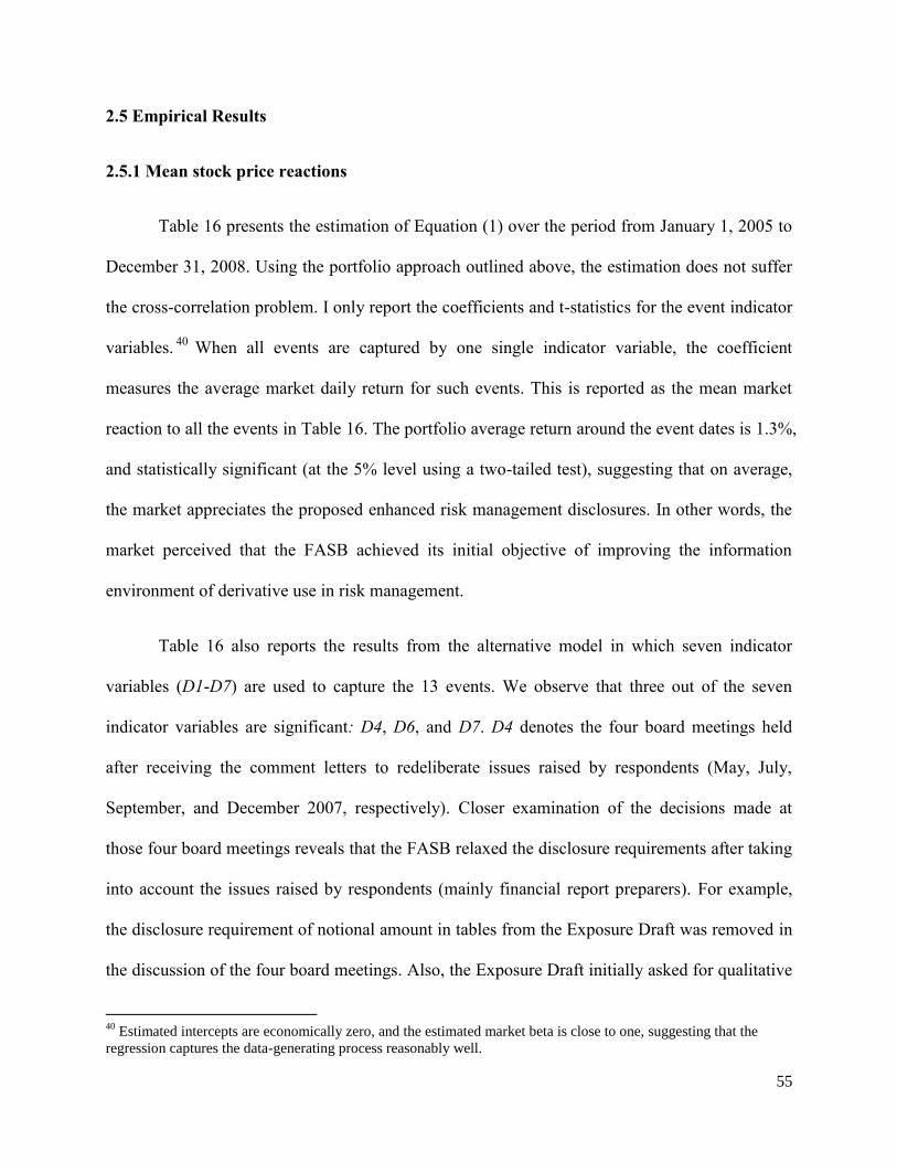
55

2.5 Empirical Results

2.5.1 Mean stock price reactions

Table 16 presents the estimation of Equation (1) over the period from January 1, 2005 to

December 31, 2008. Using the portfolio approach outlined above, the estimation does not suffer

the cross-correlation problem. I only report the coefficients and t-statistics for the event indicator

variables.40

When all events are captured by one single indicator variable, the coefficient

measures the average market daily return for such events. This is reported as the mean market

reaction to all the events in Table 16. The portfolio average return around the event dates is 1.3%,

and statistically significant (at the 5% level using a two-tailed test), suggesting that on average,

the market appreciates the proposed enhanced risk management disclosures. In other words, the

market perceived that the FASB achieved its initial objective of improving the information

environment of derivative use in risk management.

Table 16 also reports the results from the alternative model in which seven indicator

variables (D1-D7) are used to capture the 13 events. We observe that three out of the seven

indicator variables are significant: D4, D6, and D7. D4 denotes the four board meetings held

after receiving the comment letters to redeliberate issues raised by respondents (May, July,

September, and December 2007, respectively). Closer examination of the decisions made at

those four board meetings reveals that the FASB relaxed the disclosure requirements after taking

into account the issues raised by respondents (mainly financial report preparers). For example,

the disclosure requirement of notional amount in tables from the Exposure Draft was removed in

the discussion of the four board meetings. Also, the Exposure Draft initially asked for qualitative

40

Estimated intercepts are economically zero, and the estimated market beta is close to one, suggesting that the

regression captures the data-generating process reasonably well.

56

discussion of derivative use and quantitative disclosure of fair values, gains and losses by

primary underlying risk, accounting designation, and purpose. After considering the opinions

from the comment letters in these four meetings, the board decided that such disaggregation

requirements were too great a burden and replaced them with less stringent requirements.41

The

negative and significant coefficient of D4 is consistent with investors reacting negatively to the

decisions from the board meetings of relaxing disclosure requirements, consistent with the

transparency argument.42

D6 represents the date the FASB decided to require credit derivative disclosures and

additional disclosure about the current status of the guarantee/collateral. Investors are concerned

about firms’ credit risk from their hedging activities and the positive and significant sign on D6

suggests that requiring additional disclosure is considered helpful by the market.43

D7 is when

the FASB issued clarification that SFAS 161 applies to both the fiscal year and interim periods

beginning after November 15, 2008, which means that for firms with December 31 fiscal year-

end, SFAS 161 is effective for the 10-Q for the first quarter of 2009. Before the clarification, the

users and preparers were confused about from which reporting period they should comply with

SFAS 161 and there was a misunderstanding that SFAS 161 was effective for the fiscal year

beginning after November 15, 2008. Clarifying that the regulation applies to both fiscal year and

interim periods means that SFAS 161 is effective sooner than people originally thought it would

41

Specifically, the disclosure requirements for fair value and gains/losses related to derivatives were relaxed so that

the amounts should only be presented separately for derivatives designated and not designated as hedging

instruments, instead of further by primary underlying risk, accounting designation, and purpose. 42

Wong (1999) shows that risk exposure is associated with disaggregated disclosures about notional amount and fair

value of foreign exchange derivatives, suggesting that users of financial statements use this information to perform a

complete exposure assessment. 43

For the airline industry, profit margins are extremely low, and defaults by counterparties could trigger financial

distress easily.

57

be for most firms. The positive and significant sign for D7 indicates that the market welcomed

the more immediate compliance.

In contrast, we do not observe significant coefficients for D1-D3 and D5, suggesting that

these events are not associated with significant changes in investors’ expectations of the impact

of the regulations. The insignificant response around the release of SFAS 161 in March 2008

could be attributed to the four board meetings in 2007 that provide pre-emptive information

regarding the disclosure requirements.44

In summary, the market reaction tests indicate a net positive market reaction to enhanced

disclosure requirements. In the next section, I examine whether the market reactions vary

systematically with cross-sectional determinants.

2.5.2 Results of cross-sectional analyses

Table 17 reports the estimations of the portfolio time-series regressions over the same

period when all events are denoted by one indicator variable. In column (1), only the two

variables of interest are used in the cross-sectional analysis. The positive and significant

coefficient on DISC suggests that firms with higher pre-adoption risk management disclosure

experienced higher market returns. In other words, firms that had poorer pre-adoption disclosure

and thus will have to enhance their disclosure to a greater extent due to SFAS 161 are affected

negatively, consistent with the real effect argument (H2a). In addition, airlines having more of

their expected fuel consumption hedged (SCOPE) experience less positive (more negative) stock

44

The significance of market returns depends on how much of the information is unexpected, and the magnitude of

the wealth impact from the event. Thus it is not surprising to find that some events don’t have significant market

responses. For example, among the 21 events leading up to SFAS 115 identified in Beatty et al. (1996), three events

have significant market reactions around them. Similarly, depending on the specification only 3-4 out of the 17

events leading up to SOX from Zhang (2007) and 1-3 events out of the 9 leading up to SFAS 123R in Dou et al.

(2013) have significant returns around them. What they do find is that (1) the mean returns for all events are

significant, and (2) the returns around the most significant and unexpected events are significant.

58

returns around the event dates, consistent with the real effect theory that enhanced disclosure

firms using hedging more heavily could suffer from consequences of enhanced disclosure (H2b).

In Columns (2)-(4) of Table 17, I include additional control variables (one control

variable one at a time due to their high correlations) to capture the possibility that the market

reactions to enhanced risk management disclosure may vary with a firm’s ability to hedge. The

coefficient of DISC remains positive and significant for two of the three specifications, and

SCOPE is negative and significant in all the three specifications. We also observe that the three

control variables (ROA, AOCIFH, and LOWCOST) all have negative coefficients, suggesting that

shareholders of more profitable airlines, airlines with better hedging outcomes, and low-cost

carriers respond negatively to enhanced disclosure requirements.

Table 18 reports cross-sectional test results where the 13 events are captured by the 7

indicator variables. Again, Panel A is the basic specification with the two variables of interest,

and Panels B-D include control variables. Similar to results from Table 17, I find some evidence

supporting the real effects theory. For event indicators D3, D6, and D7, firms with higher pre-

adoption risk management disclosure (DISC) experienced higher market returns around such

events, and firms covering a greater portion of their expected fuel consumptions with hedging

programs (SCOPE) experience more negative (less positive) returns from enhanced disclosure

around such events.

To summarize, the cross-sectional analyses provide some support for the real effects

theory that enhanced disclosure could induce distorted hedging and production decisions, which

consequently destroy firm value. These negative effects partially offset the positive effects from

more transparent information environment.

59

2.5.3 Additional analyses and future research

The correlation table suggests that DISC and SCOPE have a relatively high correlation.

When I include them one at a time and rerun the tests, the inferences are unchanged, suggesting

that the results are not driven by multicollinearity. In addition, instead of adding control variables

one at a time, I run the complete model with all the three control variables, and the inferences for

the test variables are not affected.

My primary analyses are based on the U.S. airline industry for 2005-2008, which consists

of 41 firm-year observations with available accounting and return information. Although the

portfolio approach uses time-series regressions for the 1,007 trading dates during 2005-2008 and

small sample size is not a major concern in this case, I perform tests using model (1) with the

whole CRSP sample to see if the results from the U.S. airline industry is generalizable to the

whole sample. The results are reported in Table 19. As we can see, the average return for all the

events is not significantly different from zero. However, when I break the events into seven

indicators as in Table 16, D4 is negative and significant, and D6 is positively significant (for the

U.S. airline industry sample, D4 is negatively significant, and D6 and D7 are positively

significant). The weaker results for the whole CRSP universe sample is likely due to the fact that

compared to the airline industry where using derivatives for hedging is very common and

important, the average CRSP firms do not employ derivatives as intensively, thus they are not

affected by SFAS 161 as much as are airlines.

The cross-sectional analyses provide some initial evidence on the economic

consequences of enhanced disclosure: investors expect value-destroying decisions due to more

disclosure requirements. To further explore this theory, by examining the hedging and

60

production decisions, as well as risk exposure before and after the adoption SFAS 161, future

research can seek more evidence on how enhanced disclosure could change real actions.

2.6 Conclusions

In this paper, I examine the stock market reactions to the key events leading up to the

adoption of SFAS 161 to provide empirical evidence on the economic impact of enhanced risk

management disclosure. Focusing on the U.S. airline industry where fuel price risk management

is common and essential, I document strong positive stock returns around key event dates,

suggesting that the benefits from more transparent disclosure dominates other potential costs. My

cross-sectional analyses provide some initial evidence supporting the real effects theory of

enhanced risk management disclosure. Firms that had to increase their disclosure levels and that

had a greater portion of their expected fuel consumptions hedged experienced less positive

market reactions around the key events leading up to SFAS 161. These results suggest that

despite the desirable benefits from a better information environment, standard setters should also

weight the costs from distorted hedging and production decisions from enhanced disclosure

requirements.

61

REFERENCES

Aguirregabiria, V. and C-Y. Ho. 2012. A dynamic oligopoly game of the U.S. airline industry:

Estimation and policy experiments. Journal of Econometrics 168 (1): 156-173.

Ahmed, A., E. Kilic, and G. Lobo. 2006. Does recognition versus disclosure matter? Evidence

from value-relevance of banks’ recognized and disclosed derivative financial instruments.

The Accounting Review 81: 567-588.

Ahmed, A., E. Kilic, and G. Lobo. 2011. Effects of SFAS 133 on risk relevance of accounting

measures of banks’ derivative exposure. The Accounting Review 86: 769-804.

Ali, A., S. Klasa, and E. Yeung. 2009. The limitations of industry concentration measures

constructed with Compustat data: Implications for finance research. Review of Financial

Studies 22 (10): 3839-3871.

Allayannis, G and J.P. Weston. 2001. The use of foreign currency derivatives and firm market

value. Review of Financial Studies 14 (1): 243-276.

Bailey, E. E. and J. C. Panzar. 1981. The contestability of airline markets during the transition to

deregulation. Law and Contemporary Problems 44 (1): 125-145.

Bamber, L. S., and Y. S. Cheon. 1998. Discretionary Management Earnings Forecast Disclosures:

Antecedents and Outcomes Associated with Forecast Venue and Forecast Specificity

Choices. Journal of Accounting Research 36 (2): 167-190.

Bartram, S. M., G. W. Brown, and F. R. Fehle. 2009. International evidence on financial

derivatives usage. Financial Management 38 (1): 185-206.

Bartram, S. M., G. W. Brown, and J. Conrad. 2011. The effects of derivatives on firm risk and

value. Journal of Financial and Quantitative Analysis 46 (4): 967-999.

Bens, D., P. Berger, and S. Monahan. 2011. Discretionary disclosure in financial reporting: an

examination comparing internal firm data to externally reported segment data. The

Accounting Review 86: 417-449.

Berger, P. G., and R. N. Hann. 2007. Segment Profitability and the Proprietary and Agency

Costs of Disclosure. The Accounting Review 82 (4): 869-906.

Berry, S. 1990. Airport presence as product differentiation. American Economic Review 80:394-

399.

Berry, S. 1992. Estimation of a model of entry in the airline industry. Econometrica 60: 889-917.

Berry, S., M. Carnall, and P. Spiller. 2006. Airline hubs: costs, markups and the implications of

customer heterogeneity. Advances in Airline Economics. Vol. 1: Competition Policy and

Antitrust 183-214.

Beatty, A. S. Chamberlain, and J. Magliolo. 1996. An empirical analysis of the economic

implications of fair value accounting for investment securities. Journal of Accounting and

Economics 22: 43-77.

Beyer, A., D. A. Cohen, T. Z. Lys, and B. R. Walther. 2010. The financial reporting environment:

Review of recent literature. Journal of Accounting and Economics 50 (2-3): 296-343.

Bhamornsiri, S. and R. Schroeder. 2004. The disclosure of information on derivatives under

SFAS No. 133: Evidence from the Dow 30. Managerial Auditing Journal 19 (5): 669-

680.

Bhojraj, S., W. G. Blacconiero, and J. D. D’Souza. 2004. Voluntary disclosure in a multi-

audience setting: An empirical investigation. The Accounting Review 79 (4): 921-947.

Boguslaski, C.,H. Ito, and D. Lee. 2004. Entry patterns in the Southwest Airlines Route System.

Review of Industrial Organization 25: 317-350.

62

Borenstein, S. 1989. Hubs and high fares: Dominance and market power in the U.S. airline

industry. Rand Journal of Economics 20 (30): 344-365.

Borenstein, S., and N. Rose. 1994. Competition and price dispersion in the U.S. airline industry.

Journal of Political Economy 102 (4): 653-683.

Bova, F., Y. Dou, and O-K. Hope. 2013. Employee Ownership and Firm Disclosure. Working

paper, University of Toronto and New York University.

Brander, J. A. and A. Zhang. 1990. Market Conduct in the Airline Industry: an Empirical

Investigation. Rand Journal of Economic 21: 567-583.

Busse, M. 2002. Firm Financial Condition and Airline Price Wars. Rand Journal of Economics

33: 298-318.

Campbell, J.L. 2013. The fair value of cash flow hedges, future profitability and stock returns.

Working paper, University of Georgia.

Campello, M., C. Lin, Y. Ma, and H. Zou. 2011. The real and financial implications of corporate

hedging. Journal of Finance 66 (5): 1615-1647.

Carter, D., D. Rogers, and B. Simkins. 2006a. Hedging and value in the U.S. Airline Industry.

Journal of Applied Corporate Finance 18 (4): 21-33.

Carter, D., D. Rogers, and B. Simkins. 2006b. Does hedging affect firm value? Evidence from

the US airline industry. Financial Management Spring: 53-86.

Carter, D., D. Rogers, and B. Simkins. 2006c. Fuel hedging in the Airline Industry: The case of

Southwest Airlines. Working Paper Series. Oklahoma State University.

Chang, Y-H, and P-C Shao. 2011. Operating cost control strategies for airlines. African Journal

of Business Management 5 (26): 10396-10409.

Chen, W., H-T. Tan, and E. Y. Wang. 2012. Fair value accounting and managers’ hedging

decisions. Journal of Accounting Research 51 (1): 67-103.

Ciliberto, F. and E. Tamer. 2009. Market structure and multiple equilibria in airline markets.

Econometrica 77: 1791–1828.

Clubley, Sally. 1999. An Early Take Off. Risk May.

Darrough, M. and N. Stoughton. 1990, Financial disclosure policy in an entry game, Journal of

Accounting and Economics 12: 219–43.

Darrough, M. 1993. Disclosure policy and competition: Cournot vs. Bertrand. The Accounting

Review 68 (3): 534-561.

Dedman, E. and C. Lennox. 2009. Perceived competition, profitability and the withholding of

information about sales and the cost of sales. Journal of Accounting and Economics 48

(2-3): 210-230.

DeMarzo, P, and D. Duffie. 1995. Corporate incentives for hedging and hedge accounting.

Review of Financial Studies 8 (3): 743-771.

Dou, Y., M. H. F. Wong, and B. Xin. 2013. Evidence on the real effects of accounting: The case

of employee stock option expensing. Working paper. New York University and

University of Toronto.

Ellis, J. A., C. E. Fee, and S. E. Thomas. 2012. Proprietary costs and the disclosure of

information about customers. Journal of Accounting Research. 50 (3): 685-727.

FASB, 1990. Statement of Financial Accounting Standards No. 105, Disclosure of Information

about Financial Instruments with Off-Balance-Sheet Risk and Financial Instruments with

Concentrations of Credit Risk

FASB, 1991. Statement of Financial Accounting Standards No. 107, Disclosures about Fair

Value of Financial Instruments

63

FASB, 1994. Statement of Financial Accounting Standards No. 119, Disclosure about Derivative

Financial Instruments and Fair Value of Financial Instruments

FASB 1999. Statement of financial accounting standards No. 133, Accounting for derivative

instruments and hedging activities.

FASB 2008. Statement of financial accounting standards No. 161, Disclosures about derivative

instruments and hedging activities.

Feltham, G., F. Gigler, and J. Hughes. 1992. The effects of line-of-business reporting on

competition in oligopoly settings. Contemporary Accounting Research 9 (1): 1-23.

Froot, K., D. S. Scharfstein, and J. C. Stein. 1993. Risk management coordinating corporate

investment and financing policies. Journal of Finance 48: 1629-1658.

Gal-Or, E. 1985. Information sharing in Oligopoly. Econometrica 3 (2): 329-343.

Gal-Or, E. 1986. Information transmission—Cournot and Bertrand Equilibria. Review of

Economic Studies LIII: 85-92.

Geczy, C., B. A. Minton, and C. Schrand. 1997. Why firms use currency derivatives. Journal of

Finance 52: 1323-1354.

Gerardi, K and A. H. Shapiro. 2009. Does competition reduce price dispersion? New evidence

from the airline industry. Journal of Political Economy 117 (1): 1-37.

Gigler, F., C. Kanodia, and R. Venugopalan. 2007. Assessing the information content of mark-

to-market accounting with mixed attributes: The case of cash flow hedges. Journal of

Accounting Research 45 (2): 257-276.

Goolsbee, A. and C. Syverson. 2008. How do incumbents respond to the threat of entry?

Evidence from the major airlines. The Quarterly Journal of Economics 123 (4): 1611-

1633.

Guo, R., B. Lev, and N. Zhou. 2004. Competitive Costs of Disclosure by Biotech IPOs. Journal

of Accounting Research 42 (2): 319-355.

Harris, M. S. 1998. The association between competition and managers’ business segment

reporting decisions. Journal of Accounting Research 36: 111-128.

Haushalter, G. D. 2000. Financing policy, basis risk, and corporate hedging: Evidence from oil

and gas producers. Journal of Finance 55: 107-152.

Hayes, K. and L. Ross. 1998. Is airline price dispersion the result of careful planning or

competitive forces? Review of Industrial Organization 13: 523-542.

Healy, P. M., and K. G. Palepu. 2001. Information asymmetry, corporate disclosure, and the

capital market: A review of the empirical disclosure literature. Journal of Accounting and

Economics 31 (1-3): 405-440.

Hughes, J., J. Kao, and M. Williams. 2002. Public disclosure of forward contracts and revelation

of proprietary information. Review of Accounting Studies 7: 459-478.

Hurdle, G. J., R. L. Johnson, A. S. Joskow, G. J. Werden, and M. A. Williams. 1989.

Concentration, potential entry, and performance in the airline industry. Journal of

Industrial Economics 38 (2): 119-139.

Jones, D. A., and K. J. Smith. 2011. Comparing the value relevance, predictive value, and

persistence of other comprehensive income and special items. The Accounting Review 86

(6): 2047-2073.

Jorion, P. 2002. How informative are Value-at-Risk disclosures? The Accounting Review 77 (4):

911-931.

Kanodia, C., A. Mukherji, H. Sapra, and R. Venugopalan. 2000. Hedge disclosures, future prices,

and production distortions. Journal of Accounting Research 38 (Supplement): 53-82.

64

Kawaller, I.G. 2004. What analysts need to know about accounting for derivatives? Financial

Analysts Journal 60 (2): 24-30.

Karuna, C. 2010. Discussion of “The impact of product market competition on the quantity and

quality of voluntary disclosures”. Review of Accounting Studies 15: 712-723.

Lang, M., K. Lins, and M. Maffett. 2012. Transparency, liquidity, and valuation: International

evidence on when transparency matters most. Journal of Accounting Research 50 (3):

729-774.

Larcker, D.F. and T.O. Rusticus. 2010. On the use of instrumental variables in accounting

research. Journal of Accounting and Economics 49 (3): 186-205.

Li, X. 2010. The impacts of product market competition on the quantity and quality of voluntary

disclosures. Review of Accounting Studies 15: 663-711.

Linsmeier, T. J., and N. D. Pearson 1997. Quantitative disclosure of market risk in the SEC

release. Accounting Horizon 11 (1): 107-135.

Mackay, P and S. B. Moeller. 2007. The value of corporate risk management. Journal of Finance

62 (3): 1379-1419.

Makar, S., L. Wang, and P. Alam. The mixed attribute model in SFAS 133 cash flow hedge

accounting: Implications for the market pricing. Review of Accounting Studies 18 (1): 66-

94.

Marshall, A. and P. Weetman. 2007. Modelling transparency in disclosure: The case of foreign

exchange risk management. Journal of Business, Finance & Accounting 34 (5-6): 705-

739.

Melumad, N. D., G. Weyns, and A. Ziv. 1999. Comparing Alternative Hedge Accounting

Standards: Shareholders’ Perspective. Review of Accounting Studies 4 (3-4): 265-292.

Milgrom, P., and J. Roberts. 1982. Limited pricing and entry under incomplete information: An

equilibrium analysis. Econometrica 50 (2): 443-459.

Miller, M. H. and C. L. Culp. 1996. The SEC’s Costly Disclosure Rules. Wall Street Journal

June.

Morrell, P. and W. Swan. 2006. Airline Jet Fuel Hedging: Theory and practice. Transport

Reviews 26 (6): 713-730.

Morrison, S. A. and C. Winston. 1987. Empirical implications and tests of the contestability

hypothesis. Journal of Law and Economics 30: 53-66.

Morrison, S. A. and C. Winston. 1995. The Evolution of the Airline Industry. Brookings.

Washington, D.C.

Neven, D. J., L.-H. Roller, and Z. Zhang. 1998. Union Power and Product Market Competition:

Evidence from the Airline Industry. Centre for Economic Policy Research Discussion

Paper No. 1912.

Norton, E. C., H. Wang, and C. Ai. 2004. Computing interaction effects and standard errors in

logit and probit models. The Stata Journal 4 (2): 154-167.

Oliveira, A. 2008. An empirical model of low-cost carrier entry. Transportation Research Part A

42: 673-695.

Panaretou, A., M. B. Shackleton, and P. A. Taylor. 2013. Corporate risk management and hedge

accounting. Contemporary Accounting Research 30 (1): 116-139.

Perignon, C. and D. R. Smith. 2010. The level and quality of Value-at-Risk disclosure by

commercial banks. Journal of Banking & Finance 34 (2): 362-377.

Rajan, R. G., and L. Zingales. 1998. Financial dependence and growth. American Economic

Review 88 (3): 559-586.

65

Riley Jr., R.A., T. A. Pearson, and G. Trompeter. 2003. The value relevance of non-financial

performance variables and accounting information: the case of the airline industry.

Journal of Accounting and Public Policy 22 (3): 231-254.

Salop, S.C. 1979. Strategic entry deterrence. American Economic Review 69 (2): 335-338.

Sankar, M. R. 1995. Disclosure of Predecision Information in a Duopoly. Contemporary

Accounting Research 11: 829–859.

Seow, G.S, and K. Tam. 2002. The Usefulness of Derivative-Related Accounting Disclosures.

Review of Quantitative Finance and Accounting 18 (3): 273-291.

Sinclair, R. A. 1995. An empirical model of entry and exit in airline markets. Review of

Industrial Organization 10 (5): 541-557.

Sapra, H. 2002. Do mandatory hedge disclosures discourage or encourage excessive speculation?

Journal of Accounting Research 40 (3): 933-963.

Sefcik, S. E., and R. Thompson. 1986. An approach to statistical inference in cross-sectional

models with security abnormal returns as dependent variable. Journal of Accounting and

Research 24 (2): 316-334.

Stock, J.H., J.H. Wright, and M. Yogo. 2002. A survey of weak instruments and weak

identification in generalized method of moments. Journal of Business & Economics

Statistics 20: 518–529.

Venkatachalam, M. 1996. Value relevance of banks’ derivative disclosures. Journal of

Accounting and Economics 22 (1-3): 327-355.

Verrecchia, R. 1983. Discretionary Disclosure. Journal of Accounting and Economics 5: 365-380.

Verrecchia, R. 1990. Endogenous proprietary costs through firm interdependence. Journal of

Accounting and Economics 12: 245-250.

Verrecchia, R. E. and J. Weber. 2006. Redacted disclosure. Journal of Accounting Research 44:

791-814.

Vives, X. 1984. Duopoly information equilibrium; Cournot and Bertrand. Journal of Economic

Theory 34: 71-94.

Vives, X. 1990. Trade association disclosure rules, incentives to share information, and welfare.

RAND Journal of Economics 21 (3): 409-430.

Wong, M. H. F. 1999. The association between SFAS 119 derivatives disclosures and the foreign

exchange risk exposure of manufacturing firms. Journal of Accounting Research 38 (2):

387-417.

Zhang, H. 2009. Effect of derivative accounting rules on corporate risk management behavior.

Journal of Accounting and Economics 47: 244-264.

Zhang, I. X. 2007. Economic consequences of the Sarbanes-Oxley Act of 2002. Journal of

Accounting and Economics 44: 74-115.

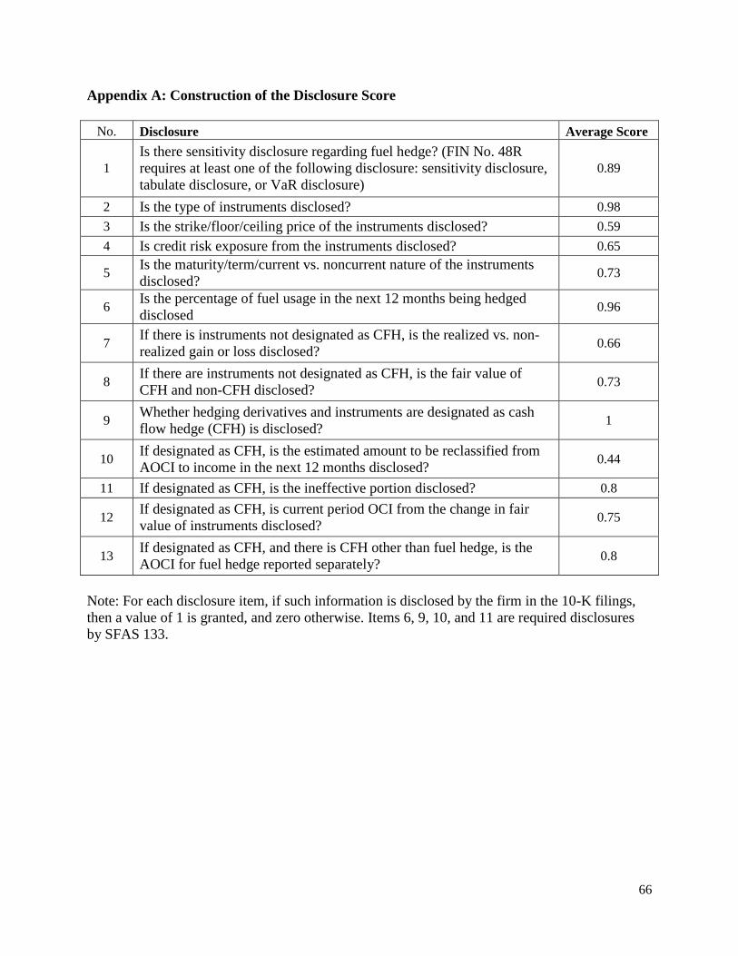
66

Appendix A: Construction of the Disclosure Score

No. Disclosure Average Score

1

Is there sensitivity disclosure regarding fuel hedge? (FIN No. 48R

requires at least one of the following disclosure: sensitivity disclosure,

tabulate disclosure, or VaR disclosure)

0.89

2 Is the type of instruments disclosed? 0.98

3 Is the strike/floor/ceiling price of the instruments disclosed? 0.59

4 Is credit risk exposure from the instruments disclosed? 0.65

5 Is the maturity/term/current vs. noncurrent nature of the instruments

disclosed? 0.73

6 Is the percentage of fuel usage in the next 12 months being hedged

disclosed 0.96

7 If there is instruments not designated as CFH, is the realized vs. non-

realized gain or loss disclosed? 0.66

8 If there are instruments not designated as CFH, is the fair value of

CFH and non-CFH disclosed? 0.73

9 Whether hedging derivatives and instruments are designated as cash

flow hedge (CFH) is disclosed? 1

10 If designated as CFH, is the estimated amount to be reclassified from

AOCI to income in the next 12 months disclosed? 0.44

11 If designated as CFH, is the ineffective portion disclosed? 0.8

12 If designated as CFH, is current period OCI from the change in fair

value of instruments disclosed? 0.75

13 If designated as CFH, and there is CFH other than fuel hedge, is the

AOCI for fuel hedge reported separately? 0.8

Note: For each disclosure item, if such information is disclosed by the firm in the 10-K filings,

then a value of 1 is granted, and zero otherwise. Items 6, 9, 10, and 11 are required disclosures

by SFAS 133.

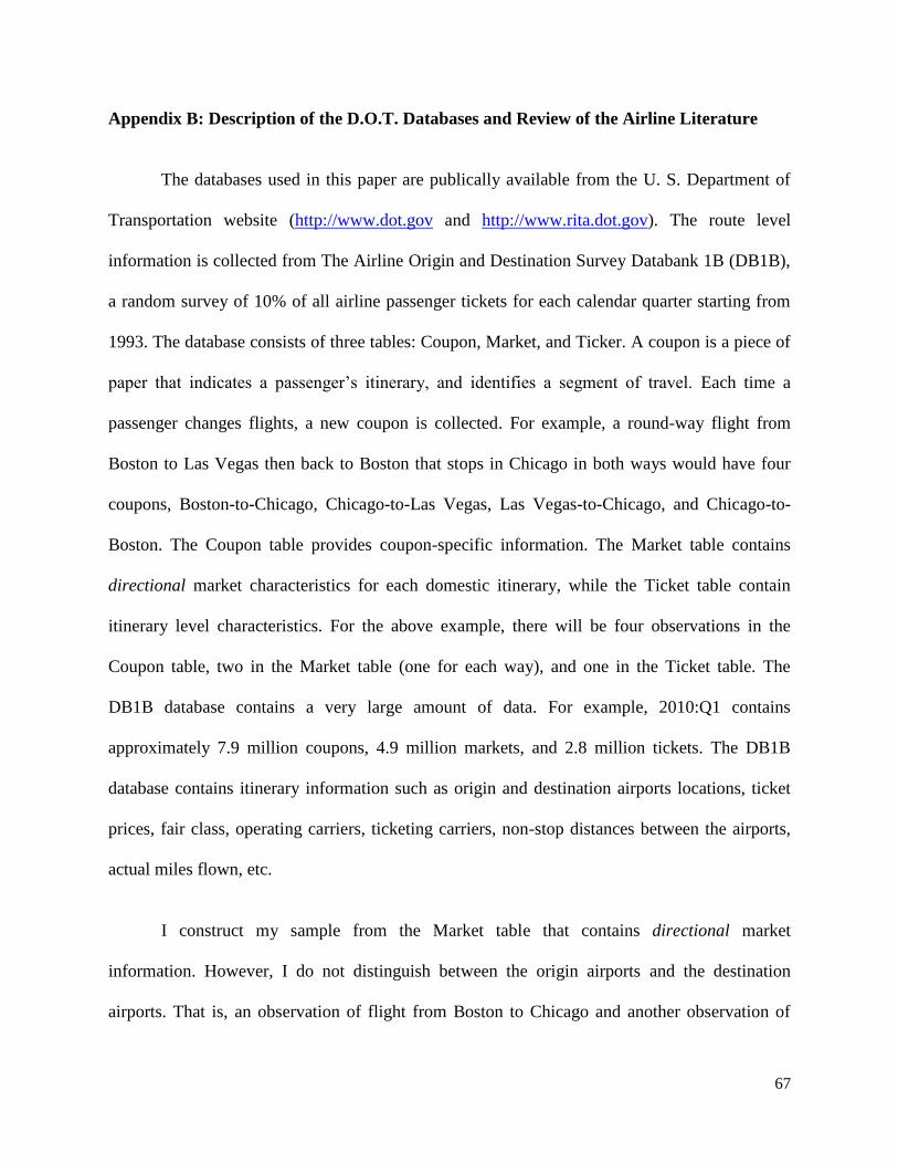
67

Appendix B: Description of the D.O.T. Databases and Review of the Airline Literature

The databases used in this paper are publically available from the U. S. Department of

Transportation website (http://www.dot.gov and http://www.rita.dot.gov). The route level

information is collected from The Airline Origin and Destination Survey Databank 1B (DB1B),

a random survey of 10% of all airline passenger tickets for each calendar quarter starting from

1993. The database consists of three tables: Coupon, Market, and Ticker. A coupon is a piece of

paper that indicates a passenger’s itinerary, and identifies a segment of travel. Each time a

passenger changes flights, a new coupon is collected. For example, a round-way flight from

Boston to Las Vegas then back to Boston that stops in Chicago in both ways would have four

coupons, Boston-to-Chicago, Chicago-to-Las Vegas, Las Vegas-to-Chicago, and Chicago-to-

Boston. The Coupon table provides coupon-specific information. The Market table contains

directional market characteristics for each domestic itinerary, while the Ticket table contain

itinerary level characteristics. For the above example, there will be four observations in the

Coupon table, two in the Market table (one for each way), and one in the Ticket table. The

DB1B database contains a very large amount of data. For example, 2010:Q1 contains

approximately 7.9 million coupons, 4.9 million markets, and 2.8 million tickets. The DB1B

database contains itinerary information such as origin and destination airports locations, ticket

prices, fair class, operating carriers, ticketing carriers, non-stop distances between the airports,

actual miles flown, etc.

I construct my sample from the Market table that contains directional market

information. However, I do not distinguish between the origin airports and the destination

airports. That is, an observation of flight from Boston to Chicago and another observation of

68

flight from Chicago to Boston from the Market table are treated as belonging to the same route

Boston-Chicago. The DB1B also provides information regarding the fare class of each ticket.

Each ticket is labeled as either coach-class, business-class, or first-class, and I eliminate all first-

class and business-class itineraries. I then eliminate airport pairs with non-stop distances greater

than 3,000 miles or shorter than 100 miles to make the sample more representative of the most

common travel pattern. I further eliminate directional flights with more than two coupons to

make sure that incumbents are clearly identified. Travels with ticketing carriers different from

operating carriers represent code sharing among airlines. Removing them gives me a cleaner

sample of incumbents and potential entrants, who are actually competing instead of forming

alliances. After eliminating these unreliable observations, I calculate the number of passengers

transported by each carrier for each quarter and delete any carriers with quarterly observation

fewer than 100 (given that the dataset is 10% random survey of all tickets, 100 DB1B

observations translates into an actual 1,000 passengers each quarter, or 8 passengers daily).

These carriers are unlikely to be valid competitors. After aggregating the data to quarter-route-

carrier level, I identify incumbents and potential entrants for each calendar quarter, and if a

potential entrant starts to operate the route for at least three out of the four quarters of a year, the

potential entrant is considered to have entered the market. However, the DB1B does not provide

the number of seats available information for each route-carrier. I obtain such information from

the T100 tables.

The Economics and Industrial Organization literature has a long history of using the

airline industry to investigate the competition dynamics and test various theories. As a matter of

fact, studies by academic economists were a significant force in the movement towards

deregulation of the domestic airline industry in the early 1970s. Since the deregulation,

69

economists have continued intensive study of the industry, in part because of the unusual

availability of reliable firm- and transaction-level data. The other reason that the airline industry

is of particular interests to researchers is that the tactics, strategies, and results of competition in

this dynamic, complex, and innovative service industry have provided a rare opportunity to

learn about the market process.

Many of the earlier studies centered on the contestability theory which suggests that the

disciplining effect of potential competition (if the costs of entry and exit are low) will result in

competitive markets so that the number of actual competitors should have no effect on prices.

With the airports and carriers information from DB1B and its proceeding form DB1A,

researchers demonstrate that an airline can enter a new market quickly and with low cost,

especially if the entrant already serves one or both of the endpoints of the route (Bailey and

Panzar 1981), and that most of the new market entries were from new competitors already

serving at least one of the points (Berry 1992).

However, potential competition appears to be no perfect substitute for actual competition,

and there emerged a fair amount of studies exploring the effects form both potential competition

and exiting competitors on price levels and dispersion using the DB1B data (Morrison and

Winston 1987; Borenstein 1989; Borenstein and Rose 1994; Goolsbee and Syverson 2008;

Gerardi and Shapiro 2009). In addition, determinants of entry decisions and exit decisions are

examined with the DB1B data in Sinclair (1995), Boguslaski et al. (2004), and Oliveria (2008)

where entry and exit are considered proxies for profitability. In this paper I extend the entry

decision models by allowing firm-specific signals as determinants in addition to traditional

market characteristics.

70

Appendix C: Journal Entries related to Cash Flow Hedges

This appendix provides an example of the journal entries associated with an investment in an

option derivative that is designated as a cash flow hedge under SFAS 133.

Date=October 2012

The firm buys jet fuel option hedge for $1,000 cash to cover a future fuel purchase and expected

consumption currently worth $6,000.

Dr Investment in Option $1,000

Cr Cash $1,000

Balance sheet Amount Income Statement Amount

Cash ($1,000)

Investment in Option $1,000

Date=December 2012

The underlying price of the option (jet fuel) goes up and hedge increases in value by $1,500.

The accounting period is completed and statements are presented.

Dr Investment in Option $1,500

Cr OCI—CFH derivative gain $1,500

Dr OCI—CFH derivative gain $1,500

Cr AOCI—CFH derivative gain $1,500

Balance sheet Amount Income Statement Amount

Cash ($1,000)

Investment Option $2,500

AOCI—CFH derivatives ($1,500)

Date= March 2013

The underlying price of the option (jet fuel) goes up and the hedge increases in value by $500.

The firm sells the hedge for $3,000 and purchases jet fuel at the current value of $8,000

($6,000+$1,500+$500).

Dr Investment in Option $500

Cr OCI—CFH derivative gain $500

Dr OCI—CFH derivative gain $500

71

Cr AOCI—CFH derivative gain $500

Dr Cash $3,000

Cr Investment in Option $3,000

Dr Inventory $8,000

Cr Cash $8,000

Balance sheet Amount Income Statement Amount

Cash ($6,000)

Investment on Option --

Inventory $8,000

AOCI—CFH derivatives ($2,000)

Date=March 2013

The firm consumes the jet fuel in providing services, and releases gain from AOCI, resulting in

fuel expenses of $5,000.

Dr Fuel Expenses $8,000

Cr Inventory $8,000

Dr AOCI—CFH derivative gains $2,000

Cr Fuel Expenses $2,000

Balance sheet Amount Income Statement Amount

Cash ($5,000)

Investment in Option --

Inventory -- Fuel Expenses $8,000

AOCI—CFH derivatives -- Fuel Expenses ($2,000)

Net Fuel Expenses $6,000

72

Appendix D: Summary of SFAS 133 Disclosure Requirements

The following must be disclosed by all reporting entities that use derivative instruments

(Paragraph 44)

Objectives for using each derivative, whether for hedging or for speculation

The context needed to understand objectives.

Qualitative disclosures are encouraged.

The following must be disclosed if derivatives are used in hedging relationships (Paragraph 45)

Risk management policies must be specified, identifying exposures to be hedged and

hedging strategies for managing the associated risks.

Identification of the type of hedging relationship (i.e., fair value, cash flow, net

investment in foreign operation), if applicable.

The hedged item must be explicitly identified.

Ineffective hedge results must be disclosed.

Any component of the derivatives’ results that is excluded from the hedge effectiveness

assessment must be disclosed.

Specific requirements for cash flow hedges (Paragraph 45b)

A description of the conditions that will result in the reclassification of accumulated

other comprehensive income into earnings, and a schedule of the estimated

reclassification expected in the coming 12 months must be disclosed.

The maximum length of time over which hedging is anticipated (except for variable

interest rate exposures) must be disclosed.

73

Entities must disclose the amount reclassified into earnings as a result of discontinued

cash flow hedges because the forecasted transaction is no longer probable.

Specific requirements for hedges of net investments in foreign operations (Paragraph 45c)

Entities must disclose the amount of the derivatives’ results that is included in the

cumulative translation adjustment during the reporting period.

74

Appendix E: Summary of Events

No. Date Event/News Title Summary

1 09/03/2005 FASB Mulls Expanded Disclosure Rules For Derivatives

(Dow Jones Newswire)

Add the project to the agenda

2 06/07/2005 FASB Board Meeting Decided scope limited to SFAS 133 and

hedged items

3 19/07/2006 FASB Board Meeting Discussed the 3 objectives, counterparty credit

risk, disclosure of notional, fair value, and

gains losses by major underlying, accounting

designation

4 06/09/2006 FASB Board Meeting Discussed gross or net presentation; whether

should cover derivatives existing throughout

the period but not at the end of the period

5 18/10/2006 FASB Board Meeting Set effective date, decided tabular disclosure

format

6 08/12/2006 Exposure Draft Issued Comment letters should be received by March

2, 2007. Effective for fiscal year and interim

periods beginning after December 15, 2007

7 02/05/2007 FASB Board Meeting Summarized and discussed the issues raised in

comment letters

8 25/07/2007 FASB Board Meeting Discussed the scope and decide to retain the

same scope

9 26/09/2007 FASB Board Meeting Agreed on the revised tabular format.

10 05/12/2007 FASB Board Meeting Completed the redeliberations/relax notional

amount disclosure

11 19/03/2008 Announcement of SFAS 161 Effective for fiscal year and interim periods

beginning after November 15, 2008

12 30/04/2008 Amendments to disclosure requirements Amended credit derivative disclosures

13 12/09/2008 FASB Board Meeting and Announcement Clarified the effective date applies to both

fiscal year and interim periods

75

Appendix F: Construction of the Disclosure Score

No. Disclosure

1

Is there sensitivity disclosure regarding fuel hedge? (FIN No. 48R requires at least

one of the following disclosure: sensitivity disclosure, tabulate disclosure, or VaR

disclosure)

2 Is the type of instruments disclosed?

3 Is the strike/floor/ceiling price of the instruments disclosed?

4 Is credit risk exposure from the instruments disclosed?

5 Is the maturity/term/current vs. noncurrent nature of the instruments disclosed?

6 Is the percentage of fuel usage in the next 12 months being hedged disclosed

7 If there is instruments not designated as CFH, is the realized vs. non-realized gain or

loss disclosed?

8 If there are instruments not designated as CFH, is the fair value of CFH and non-CFH

disclosed?

9 Whether hedging derivatives and instruments are designated as cash flow hedge

(CFH) is disclosed?

10 If designated as CFH, is the estimated amount to be reclassified from AOCI to income

in the next 12 months disclosed?

11 If designated as CFH, is the ineffective portion disclosed?

12 If designated as CFH, is current period OCI from the change in fair value of

instruments disclosed?

13 If designated as CFH, and there is CFH other than fuel hedge, is the AOCI for fuel

hedge reported separately?

Note: For each disclosure item, if such information is disclosed by the firm in the 10-K filings,

then a value of 1 is granted, and zero otherwise. Items 6, 9, 10, and 11 are required disclosures

by SFAS 133.

76

Appendix G: Summary of SFAS 161 disclosure requirements

The additional disclosures required by FAS 161 are summarized below:

Entities must provide information outlining the reasons for holding or issuing derivative

instruments. Disclosures should be in the context of overall risk exposures.

For derivatives used as hedges, the organization should provide a description of those

designated as a) fair value hedges, b) cash flow hedges, and c) foreign currency hedges.

In addition, for derivatives held solely as investments, the entity needs to provide the

purpose for holding such an investment.

Qualitative information about the entity’s objectives and strategies for using derivative

instruments should be made in the context of the entity’s overall risk exposures relating

to interest risk, foreign currency exchange rate risk, commodity price risk, credit risk, and

equity price risk. If made, those disclosures should include a discussion of those

exposures even though the entity does not manage some or all the risks through the use of

these derivatives.

For each reporting period in which a statement of financial position is presented, the

following should be disclosed in tabular form by type of derivative contract:

o The location and fair value amounts of derivative instruments reported in the

statement of financial position

o The location and amount of gains and losses reported in the statement of

operations. Gains and losses should be presented separately for:

Derivative instruments designated as fair value hedges

The effective portion of gains and losses on cash flow hedges and net

investment hedges recognized in OCI

77

The effective portion of gains and losses on cash flow hedges and net

investment hedges reclassified out of OCI and into earnings

The portion of gains and losses for cash flow hedges and net investment

hedges representing a) the amount of the hedges’ ineffectiveness and b)

the amount excluded from the assessment of hedge effectiveness

Derivatives not designated as hedges

For each reporting period for which a statement of financial position is presented, the

following should be disclosed:

o The existence and nature of credit-risk-related contingent features and

circumstances that could be triggered in instruments that are in a net liability

position

o The aggregate fair value of such derivatives

o The aggregate value of assets that are already reported as collateral at the end of

the reporting period

o The aggregate fair value of additional assets that would be reported as collateral

o The aggregate fair value of assets needed to settle the instrument immediately if

credit-risk-related contingent features were triggered

78

TABLE 1: Variable Definitions—Chapter 1

VARIABLE DEFINITION

Key test variables:

I_AOCIFH Weighted average of the route-year’s all incumbents’ AOCI for fuel

hedge. AOCI is scaled by total asset before weighting.

I_DISC Weighted average of the route-years’ all incumbents’ disclosure

scores.

I_DISCD =1 when above median.

I_AOCIFH×I_DISCD The product of I_AOCIFH and I_DISCD

Incumbents’ and entrants’ characteristics

I_LF Weighted average of all incumbents’ loading factor. Loading factor is

a common performance measure of airlines = passengers carried/total

seats available

I_LEV Weighted average of all incumbents’ leverage. Leverage is calculated

as long term debt/total asset

I_SIZE Weighted average of all incumbents’ size. size=log(total asset)

I_ROA Weighted average of all incumbents’ ROA. ROA=net income/total

asset

I_LOSS Weighted average of all incumbents’ loss indicator. Loss=1 if net

income<0

I_FUELEXP Log of (1+ Weighted average of all incumbents’ fuel expense as % of

their total operating expenses).

I_LOSS Weighted average of all incumbents’ loss indicator.

I_CFO Weighted average of all incumbents’ cash flow from operation. cash

flow from operation is scaled by total asset

I_FR Weighted average of all incumbents’ percentage of international RSM

to its total RSM.

E_AOCIFH Entrant’s AOCI scaled by total asset

E_LEV Entrant’s leverage

E_SIZE Entrant’s size

E_ROA Entrant’s ROA

E_LOSS Entrant’s loss indicator variable

E_FUELEXP Log of (1 + Entrant’s fuel expense as % of total operating expenses)

E_LOSS Entrant’s loss indicator

E_CFO Entrant’s cash from operation

79

Route characteristics

ORIGININCOME The route’s origin’s income measured as log(income/1000);

DESTINCOME The route’s destination’s income

HUB Indicator variable=1 if at least one of the airports is the hub of some

airlines

HHI the HHI of the route calculated using the passengers carried by each

carrier

MKTSIZE the market size of the route, calculated as the total passengers of the

route*the distance of the route

DISTANCE The non-stop distance of the route; in thousand miles

DISTANCE2 The square of distance

DENSITY The number of passengers of the route; in thousands

DENSITY2 The square of DENSITY

MEANPOP the natural log of the mean population for both endpoint MSA

80

TABLE 2: Descriptive Statistics

Variable N mean sd p5 p50 p95 min max p25 p75

ENTRY 2,829 0.07 0.26 0.00 0.00 1.00 0.00 1.00 0.00 0.00

I_AOCIFH(%) 2,829 0.33 0.02 -2.83 0.00 4.64 -6.61 7.48 -0.26 0.13

I_SIZE 2,829 8.29 3.02 0.01 9.46 10.40 -0.15 10.71 8.49 9.89

I_ROA 2,829 -0.06 0.67 -0.24 -0.01 0.05 -19.72 0.89 -0.07 0.02

I_FUELEXP 2,829 2.66 0.94 0.01 2.95 3.47 0.00 3.97 2.55 3.13

I_CFO 2,825 0.05 0.09 -0.07 0.04 0.26 -0.44 0.34 0.00 0.09

I_LF 2,829 0.70 0.11 0.51 0.70 0.86 0.03 1.00 0.64 0.76

I_LOSS 2,829 0.53 0.49 0.00 0.89 1.00 0.00 1.00 0.00 1.00

I_LEV 2,829 0.29 0.17 0.00 0.34 0.53 0.00 0.60 0.15 0.42

E_AOCI 2,829 0.00 0.01 -0.01 0.00 0.02 -0.07 0.23 0.00 0.00

E_SIZE 2,829 9.02 1.11 7.06 9.26 10.39 -0.15 10.71 8.41 9.89

E_ROA 2,829 -0.06 0.66 -0.21 -0.01 0.05 -19.72 0.89 -0.06 0.02

E_FUELEXP 2,829 2.97 0.33 2.37 3.00 3.49 2.18 3.97 2.73 3.21

E_CFO 2,829 0.06 0.07 -0.06 0.05 0.15 -0.44 0.35 0.01 0.09

E_LOSS 2,825 0.64 0.48 0.00 1.00 1.00 0.00 1.00 0.00 1.00

E_LEV 2,829 0.36 0.12 0.08 0.38 0.54 0.00 0.60 0.30 0.45

ORIGININCOME 2,829 39.49 7.17 29.57 38.69 54.91 21.32 62.63 34.49 43.25

DESTINCOME 2,829 39.48 7.42 29.46 38.85 54.91 19.72 62.63 34.03 43.01

HUB 2,829 0.52 0.50 0.00 1.00 1.00 0.00 1.00 0.00 1.00

HHI 2,829 0.22 0.36 0.00 0.00 0.99 0.00 1.00 0.00 0.42

DISTANCE 2,829 7.54 5.80 2.16 5.81 22.95 1.00 29.94 3.49 9.25

DISTANCE2 2,829 90.47 150.63 4.67 33.76 526.70 1.00 896.40 12.18 85.56

DENSITY 2,829 23.48 26.09 2.62 13.32 75.61 1.77 190.18 5.95 31.99

DENSITY2 2,825 1231.71 3118.69 6.85 177.32 5716.42 3.12 36169.95 35.38 1023.30

MEANPOP 2,829 8.07 0.72 6.98 8.07 9.26 5.00 9.67 7.60 8.57

MKTSIZE 2,829 14.49 1.32 12.27 14.65 16.34 6.75 18.10 13.71 15.40

Notes: ORIGININCOME and DESTINCOME are in thousand dollars, DISTANCE is in hundred miles, and DENSITY is in thousands. Variable definitions are

provided in Table 1.

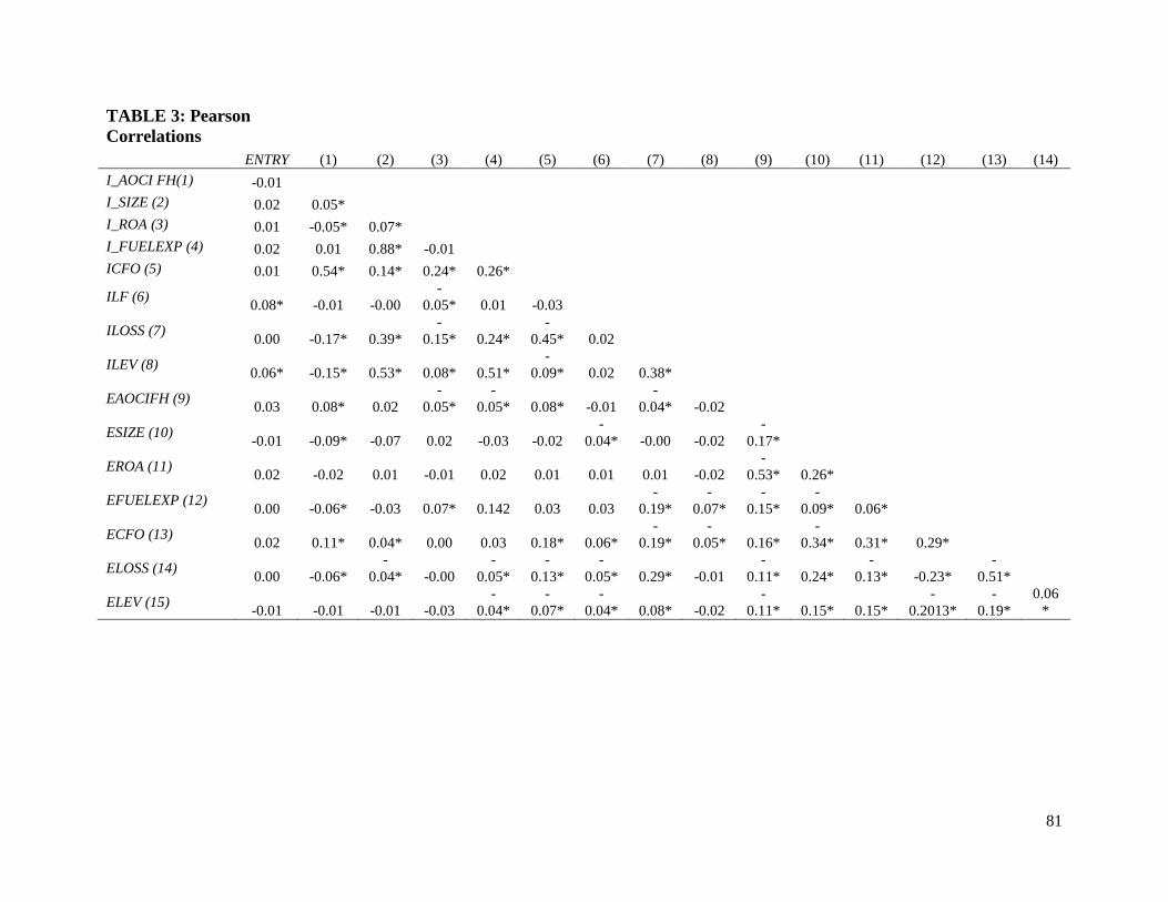
81

TABLE 3: Pearson

Correlations

ENTRY (1) (2) (3) (4) (5) (6) (7) (8) (9) (10) (11) (12) (13) (14)

I_AOCI FH(1) -0.01

I_SIZE (2) 0.02 0.05*

I_ROA (3) 0.01 -0.05* 0.07*

I_FUELEXP (4) 0.02 0.01 0.88* -0.01

ICFO (5) 0.01 0.54* 0.14* 0.24* 0.26*

ILF (6)

0.08* -0.01 -0.00

-

0.05* 0.01 -0.03

ILOSS (7)

0.00 -0.17* 0.39*

-

0.15* 0.24*

-

0.45* 0.02

ILEV (8)

0.06* -0.15* 0.53* 0.08* 0.51*

-

0.09* 0.02 0.38*

EAOCIFH (9)

0.03 0.08* 0.02

-

0.05*

-

0.05* 0.08* -0.01

-

0.04* -0.02

ESIZE (10)

-0.01 -0.09* -0.07 0.02 -0.03 -0.02

-

0.04* -0.00 -0.02

-

0.17*

EROA (11)

0.02 -0.02 0.01 -0.01 0.02 0.01 0.01 0.01 -0.02

-

0.53* 0.26*

EFUELEXP (12)

0.00 -0.06* -0.03 0.07* 0.142 0.03 0.03

-

0.19*

-

0.07*

-

0.15*

-

0.09* 0.06*

ECFO (13)

0.02 0.11* 0.04* 0.00 0.03 0.18* 0.06*

-

0.19*

-

0.05* 0.16*

-

0.34* 0.31* 0.29*

ELOSS (14)

0.00 -0.06*

-

0.04* -0.00

-

0.05*

-

0.13*

-

0.05* 0.29* -0.01

-

0.11* 0.24*

-

0.13* -0.23*

-

0.51*

ELEV (15)

-0.01 -0.01 -0.01 -0.03

-

0.04*

-

0.07*

-

0.04* 0.08* -0.02

-

0.11* 0.15* 0.15*

-

0.2013*

-

0.19*

0.06

*

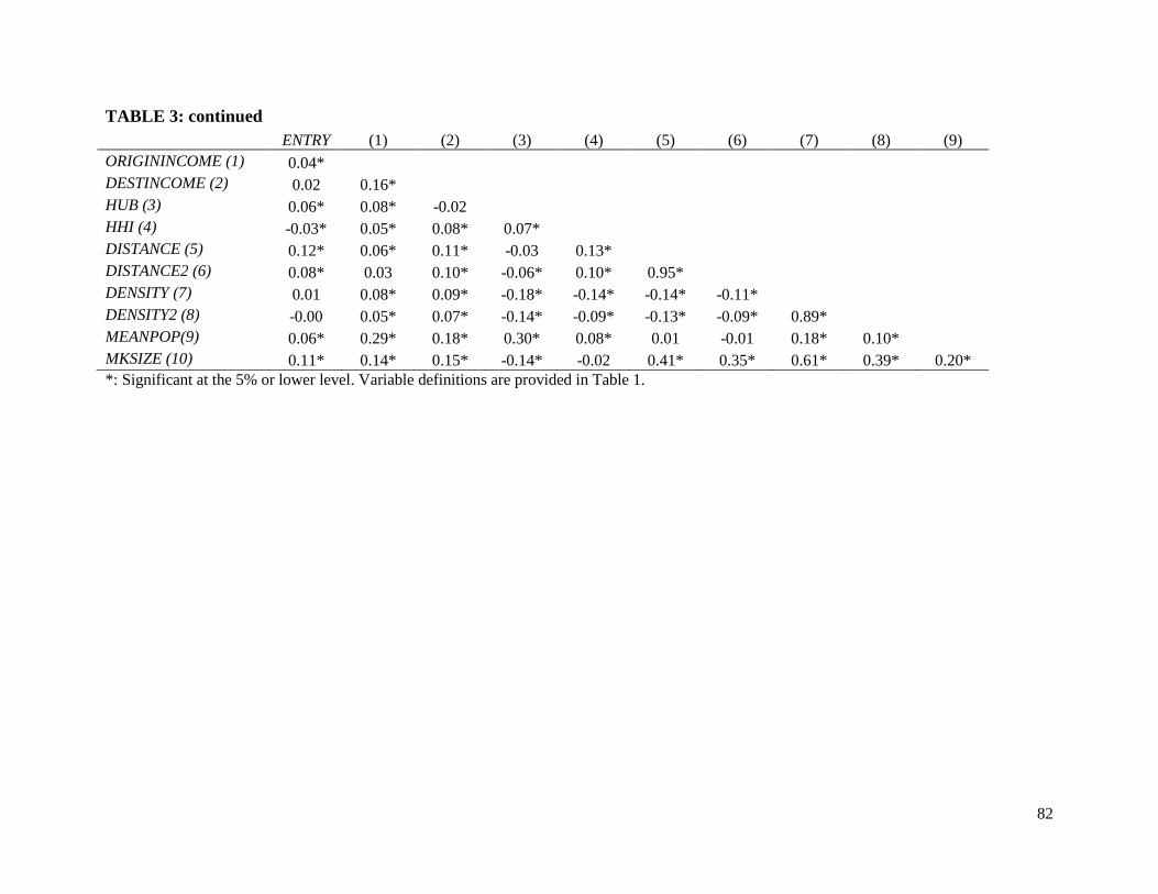
82

TABLE 3: continued

ENTRY (1) (2) (3) (4) (5) (6) (7) (8) (9)

ORIGININCOME (1) 0.04*

DESTINCOME (2) 0.02 0.16*

HUB (3) 0.06* 0.08* -0.02

HHI (4) -0.03* 0.05* 0.08* 0.07*

DISTANCE (5) 0.12* 0.06* 0.11* -0.03 0.13*

DISTANCE2 (6) 0.08* 0.03 0.10* -0.06* 0.10* 0.95*

DENSITY (7) 0.01 0.08* 0.09* -0.18* -0.14* -0.14* -0.11*

DENSITY2 (8) -0.00 0.05* 0.07* -0.14* -0.09* -0.13* -0.09* 0.89*

MEANPOP(9) 0.06* 0.29* 0.18* 0.30* 0.08* 0.01 -0.01 0.18* 0.10*

MKSIZE (10) 0.11* 0.14* 0.15* -0.14* -0.02 0.41* 0.35* 0.61* 0.39* 0.20*

*: Significant at the 5% or lower level. Variable definitions are provided in Table 1.

83

TABLE 4: The Impact of Incumbents’ AOCIFH (I_AOCIFH) and its Interaction with

Disclosure on Entry: Probit Regressions Results

(1) (2) (3) (4)

ENTRY ENTRY ENTRY ENTRY

I_AOCIFH (-) -7.747*** -8.874*** -9.040*** -8.294**

(-3.93) (-4.35) (-3.74) (-2.15)

I_AOCIFH×I_DISCD (-)

-10.376***

(-2.72)

I_DISCD

0.194

(0.74)

I_SIZE

0.054 0.071* 0.027

(1.35) (1.84) (0.32)

I_ROA

-0.204** -0.209** 0.190

(-2.30) (-2.09) (0.47)

I_FUELEXP

-0.295* -0.334* -0.349

(1.67) (-1.89) (-1.09)

I_CFO

1.077 0.817 3.620**

(1.35) (0.93) (2.36)

I_LF

0.288 0.272 0.492

(0.79) (0.72) (0.82)

I_LOSS

-0.127 -0.162 -0.141

(-0.70) (1.01) (-0.55)

I_LEV

1.142*** 1.016*** 0.937

(3.42) (2.73) (0.96)

E_AOCI3

4.923 -15.554

(0.96) (-1.10)

E_SIZE

0.041 0.184

(0.58) (1.16)

E_ROA

0.455** 0.894**

(2.43) (2.41)

E_FUELEXP

-0.610* -0.878

(-1.78) (-1.41)

E_CFO

-2.159 2.087

(-1.64) (0.82)

E_LOSS

0.255* 0.064

(1.67) (0.22)

E_LEV

0.083 -0.639

(0.30) (-0.94)

ORIGININCOME 0.000 0.000 0.000 0.000*

(0.50) (0.77) (0.98) (1.73)

DESTINCOME 0.000 0.000 0.000 -0.000

(0.49) (0.69) (0.75) (-0.04)

HUB 0.080 0.041 0.045 0.174

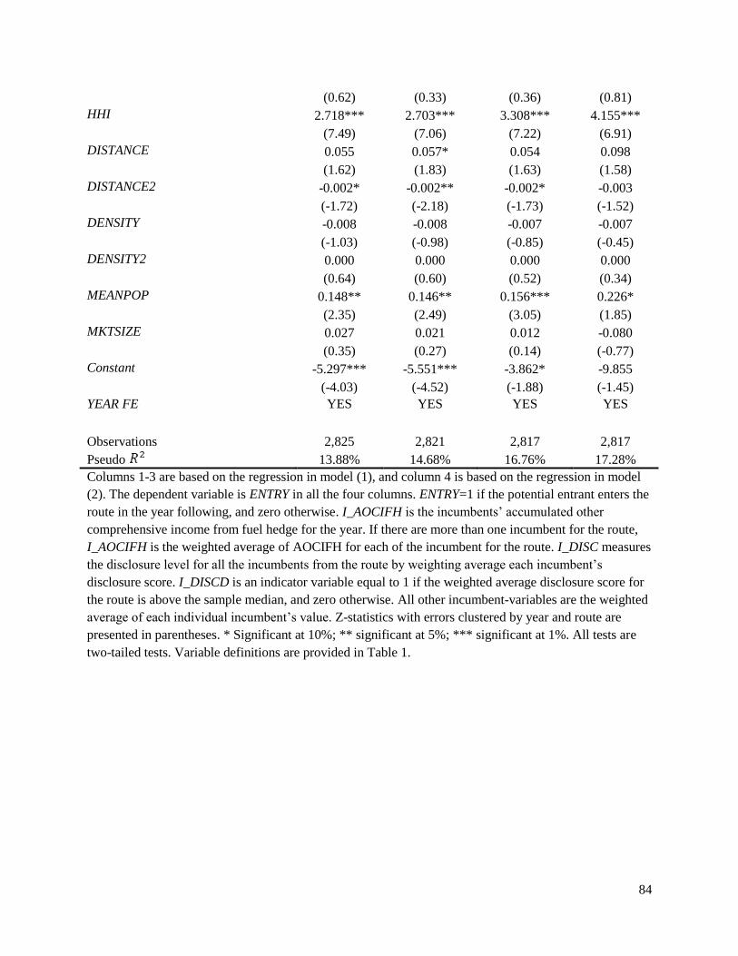
84

(0.62) (0.33) (0.36) (0.81)

HHI 2.718*** 2.703*** 3.308*** 4.155***

(7.49) (7.06) (7.22) (6.91)

DISTANCE 0.055 0.057* 0.054 0.098

(1.62) (1.83) (1.63) (1.58)

DISTANCE2 -0.002* -0.002** -0.002* -0.003

(-1.72) (-2.18) (-1.73) (-1.52)

DENSITY -0.008 -0.008 -0.007 -0.007

(-1.03) (-0.98) (-0.85) (-0.45)

DENSITY2 0.000 0.000 0.000 0.000

(0.64) (0.60) (0.52) (0.34)

MEANPOP 0.148** 0.146** 0.156*** 0.226*

(2.35) (2.49) (3.05) (1.85)

MKTSIZE 0.027 0.021 0.012 -0.080

(0.35) (0.27) (0.14) (-0.77)

Constant -5.297*** -5.551*** -3.862* -9.855

(-4.03) (-4.52) (-1.88) (-1.45)

YEAR FE YES YES YES YES

Observations 2,825 2,821 2,817 2,817

Pseudo 13.88% 14.68% 16.76% 17.28%

Columns 1-3 are based on the regression in model (1), and column 4 is based on the regression in model

(2). The dependent variable is ENTRY in all the four columns. ENTRY=1 if the potential entrant enters the

route in the year following, and zero otherwise. I_AOCIFH is the incumbents’ accumulated other

comprehensive income from fuel hedge for the year. If there are more than one incumbent for the route,

I_AOCIFH is the weighted average of AOCIFH for each of the incumbent for the route. I_DISC measures

the disclosure level for all the incumbents from the route by weighting average each incumbent’s

disclosure score. I_DISCD is an indicator variable equal to 1 if the weighted average disclosure score for

the route is above the sample median, and zero otherwise. All other incumbent-variables are the weighted

average of each individual incumbent’s value. Z-statistics with errors clustered by year and route are

presented in parentheses. * Significant at 10%; ** significant at 5%; *** significant at 1%. All tests are

two-tailed tests. Variable definitions are provided in Table 1.

85

TABLE 5: Regressing Disclosure Scores on Year Indicators

I_DISC

2002 -0.0100

(-0.29)

2003 -0.0556

(-1.64)

2004 -0.0240

(-0.74)

2005 0.0634*

(1.89)

2006 -0.0372

(-1.11)

2007 0.0038

(0.11)

2008 0.1417***

(4.04)

2009 0.1867***

(5.98)

2010 0.2972***

(5.75)

Constant 0.1920***

(7.16)

Observations 2,829

Adjusted 0.063

The table regresses the disclosure score on year indicator variables. I_DISC is the dependent

variable, measuring the incumbents’ risk management disclosure level. Value of t statistics in

parentheses. Year 2001 is the reference group.* Significant at 10%; ** significant at 5%; ***

significant at 1%. All tests are two-tailed tests.

86

TABLE 6: The Impact of Incumbents’ AOCIFH (I_AOCIFH) on Entry: Pre- and Post-

SFAS 161 comparisons: Probit Regressions Results

(1) (2)

ENTRY, PRE SFAS161 ENTRY, POST SFAS 161

I_AOCIFH(-) -11.770** -15.302***

(-2.24) (-2.92)

I_SIZE 0.079 0.261*

(1.62) (1.69)

I_ROA -0.252** 1.052

(-2.01) (1.14)

I_FUELEXP -0.340 -0.841

(-1.49) (-1.38)

I_CFO 0.486 6.086**

(0.50) (2.51)

I_LF -0.043 1.753

(-0.13) (1.36)

I_LOSS -0.331 0.699

(-1.49) (0.84)

I_LEV 0.978** 0.740

(2.20) (0.56)

E_AOCI 8.692 3.661

(1.12) (0.70)

E_SIZE 0.029 0.197

(0.36) (1.45)

E_ROA 0.477** 2.278**

(2.03) (2.08)

E_FUELEXP -0.484 -0.919***

(-1.34) (-4.17)

E_CFO -2.517* -1.007

(-1.72) (-0.19)

E_LOSS 0.303 -0.134

(1.30) (-0.54)

E_LEV -0.047 4.753***

(-0.18) (2.72)

ORIGININCOME 0.000 -0.000

(1.15) (-0.90)

DESTINCOME 0.000 0.000

(0.43) (1.53)

HUB 0.138 -0.764**

(1.00) (-2.26)

HHI 3.189*** 4.299***

(5.92) (10.37)

DISTANCE 0.040 0.134

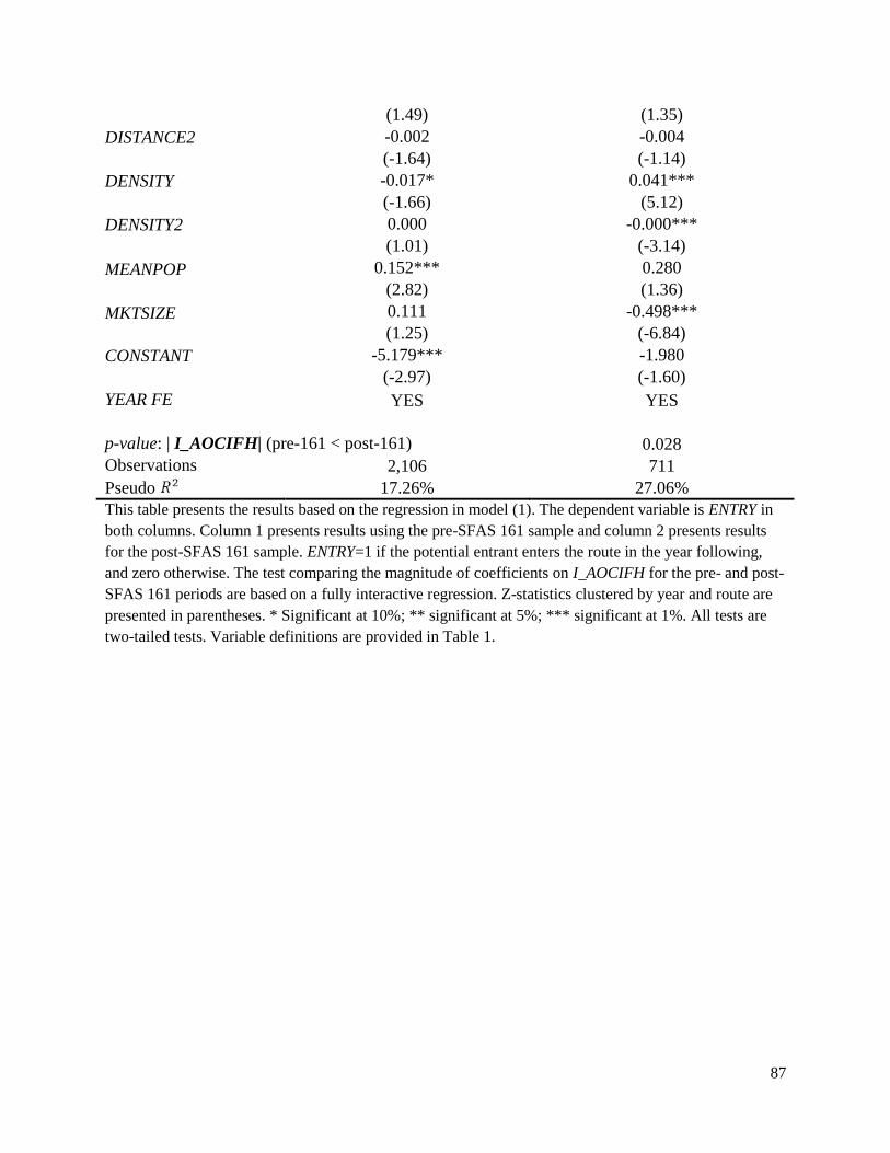
87

(1.49) (1.35)

DISTANCE2 -0.002 -0.004

(-1.64) (-1.14)

DENSITY -0.017* 0.041***

(-1.66) (5.12)

DENSITY2 0.000 -0.000***

(1.01) (-3.14)

MEANPOP 0.152*** 0.280

(2.82) (1.36)

MKTSIZE 0.111 -0.498***

(1.25) (-6.84)

CONSTANT -5.179*** -1.980

(-2.97) (-1.60)

YEAR FE YES YES

p-value: | I_AOCIFH| (pre-161 < post-161) 0.028

Observations 2,106 711

Pseudo 17.26% 27.06%

This table presents the results based on the regression in model (1). The dependent variable is ENTRY in

both columns. Column 1 presents results using the pre-SFAS 161 sample and column 2 presents results

for the post-SFAS 161 sample. ENTRY=1 if the potential entrant enters the route in the year following,

and zero otherwise. The test comparing the magnitude of coefficients on I_AOCIFH for the pre- and post-

SFAS 161 periods are based on a fully interactive regression. Z-statistics clustered by year and route are

presented in parentheses. * Significant at 10%; ** significant at 5%; *** significant at 1%. All tests are

two-tailed tests. Variable definitions are provided in Table 1.

88

TABLE 7: The Effects of Individual Disclosure Items on Entry: Probit Regressions Results

(1) (2) (3)

ENTRY ENTRY ENTRY

I_AOCIFH 9.727 7.140 32.616

(1.54) (0.29) (1.62)

I_RECLASSR -0.048 -0.049 -0.011

(-1.20) (-1.28) (-0.15)

INT_RECLASS -3.162*** -3.980** -5.551**

(-2.65) (-2.12) (-1.98)

I_OTHER 0.068 0.058

(1.20) (1.12)

INT_OTHER 0.824 0.745

(0.31) (0.45)

I_OCI 0.054

(1.00)

INT_OCI 2.788

(1.32)

I_INEFF -0.013

(-0.44)

INT_INEFF 0.272

(0.10)

I_TYPE -0.094*

(-1.91)

INT_TYPE -7.640**

(-1.97)

I_FCPRICE 0.027

(0.69)

INT_FCPRICE -0.801

(-0.39)

I_CREDIT -0.037

(-1.46)

INT_CREDIT 3.525

(1.25)

I_REALIZE -0.010

(-0.25)

INT_REALIZE -1.302

(-1.07)

I_CURRENT 0.053

(1.54)

INT_CURRENT -3.309**

(-2.07)

I_FVDISCLOSURE 0.002

(0.05)

89

INT_FVDISCLOSURE

(-0.93)

I_SIZE 0.099 0.029 0.051

(1.52) (0.38) (1.15)

I_ROA -0.632* -0.655* -0.352

(-1.66) (-1.75) (-0.73)

I_FUELEXP -0.417** -0.317* -0.325

(-2.19) (-1.72) (-1.64)

I_CFO 1.066 0.943 1.153

(1.35) (1.17) (1.15)

I_LF 0.193 0.388 0.051

(0.22) (0.42) (0.08)

I_LOSS -0.314 -0.254 -0.021

(-1.21) (-1.03) (-0.10)

I_LEV 1.424*** 1.369*** 1.096

(3.08) (2.80) (1.26)

E_AOCI 5.523 3.030 -1.001

(1.32) (0.81) (-0.17)

E_SIZE 0.099* 0.115* 0.016

(1.71) (1.66) (0.17)

E_ROA 0.174* 0.205 0.471*

(1.89) (0.78) (1.68)

E_FUELEXP -0.386 -0.344 -0.967***

(-1.37) (-1.58) (-3.57)

E_CFO -4.137*** -3.432*** -1.223

(-2.98) (-2.61) (-0.63)

E_LOSS 0.150 0.153 0.308*

(0.80) (0.68) (1.72)

E_LEV 0.956*** 1.249*** 0.132

(3.37) (4.57) (0.28)

ORIGININCOME 0.000 0.000 0.000

(1.28) (0.87) (0.67)

DESTINCOME 0.000 0.000 0.000

(1.23) (0.75) (0.49)

HUB -0.037 -0.126 -0.082

(-0.23) (-0.83) (-0.47)

HHI 4.075*** 4.029*** 3.124***

(7.29) (6.29) (5.11)

DISTANCE -0.102 -0.114 0.075

(-1.46) (-1.46) (1.20)

DISTANCE2 0.001 0.001 -0.003

(0.59) (0.54) (-1.48)

DENSITY -0.032* -0.034** -0.004

90

(-1.94) (-2.32) (-0.33)

DENSITY2 0.000 0.000 0.000

(1.24) (1.34) (0.10)

MEANPOP 0.168 0.135 0.132**

(1.59) (1.26) (1.97)

MKTSIZE 0.739*** 0.838*** 0.028

(2.87) (3.84) (0.20)

Constant -15.902*** -17.632*** -6.909

(-3.54) (-4.97) (-1.56)

YEAR FE YES YES YES

Observations 2,817 2,817 1,857

Pseudo 17.11% 17.31% 20.00%

This table shows results on how different individual disclosure items enhance the informativeness of

accounting signals differently. The dependent variable is ENTRY in all the three columns. In column 1,

the disclosure variable is I_RECLASS, indicating whether the incumbents disclose their estimated

reclassification of AOCI into net income in the next year. In column 2, I_OTHER, the variable for all

other disclosure items aggregated, is added to the regression. Column 3 presents results when more

individual disclosure items are added. ENTRY=1 if the potential entrant enters the route in the year

following, and zero otherwise. The prefix “INT_” indicates the interaction term between I_AOCIFH and

disclosure scores. Z-statistics clustered by year and route are presented in parentheses. * Significant at

10%; ** significant at 5%; *** significant at 1%. All tests are two-tailed tests. Variable definitions are

provided in Table 1.

91

TABLE 8: 2SLS for Disclosure, Using I_FR as the Instrument Variable

FIRST STAGE SECOND STAGE

ISCORED ENTRY

I_FR (+) 1.834***

(6.06)

I_AOCI (-) -6.455**

(-1.99)

I_AOCI×I_DISCDPRE (-) -10.767***

(-3.31)

I_SCOREDPRE -0.150

(-0.43)

I_SIZE 0.435*** 0.057

(12.17) (0.60)

I_ROA -0.236*** 0.047

(-5.45) (0.09)

I_FUELEXP 0.281** -0.364

(2.01) (-0.97)

I_CFO 3.147*** 3.610*

(6.95) (1.84)

I_LF 0.432 0.783

(1.52) (1.35)

I_LOSS 0.917*** -0.284

(11.38) (0.83)

I_LEV -1.183*** 1.156

(-5.78) (1.12)

E_AOCI -0.804 -16.648

(-0.27) (-1.20)

E_SIZE 0.064** 0.255

(1.99) (1.30)

E_ROA -0.101 1.134*

(1.62) (1.83)

E_FUELEXP 0.058 -1.232***

(0.44) (-3.31)

E_CFO -0.662 3.503

(1.06) (1.25)

E_LOSS -0.319*** 0.018

(-4.19) (0.04)

E_LEV 0.689*** -0.796*

(2.92) (-1.68)

ORIGININCOME 0.000*** 0.000**

(6.65) (2.13)

DESTINCOME 0.000*** -0.000

(5.43) (-0.27)

92

HUB 0.058 0.192

(0.92) (0.84)

HHI 0.399 4.459***

(1.63) (7.15)

DISTANCE -0.034 0.060

(-1.40) (0.84)

DISTANCE2 0.001 -0.002

(1.06) (-0.72)

DENSITY -0.013*** -0.014

(-2.97) (-0.76)

DENSITY2 0.000*** 0.000

(2.72) (0.54)

MEANPOP -0.044 0.247

(-0.96) (1.59)

MKTSIZE -0.024 -0.052

(-0.48) (-0.38)

CONSTANT -6.877*** -10.289

(-7.89) (-1.12)

YEAR FE YES YES

Observations 2,817 2,817

Pseudo 26.67% 17.88%

Z-statistics clustered by year and route are presented in parentheses. * Significant at 10%; ** significant

at 5%; *** significant at 1%. All tests are two-tailed tests. Variable definitions are provided in Table 1.

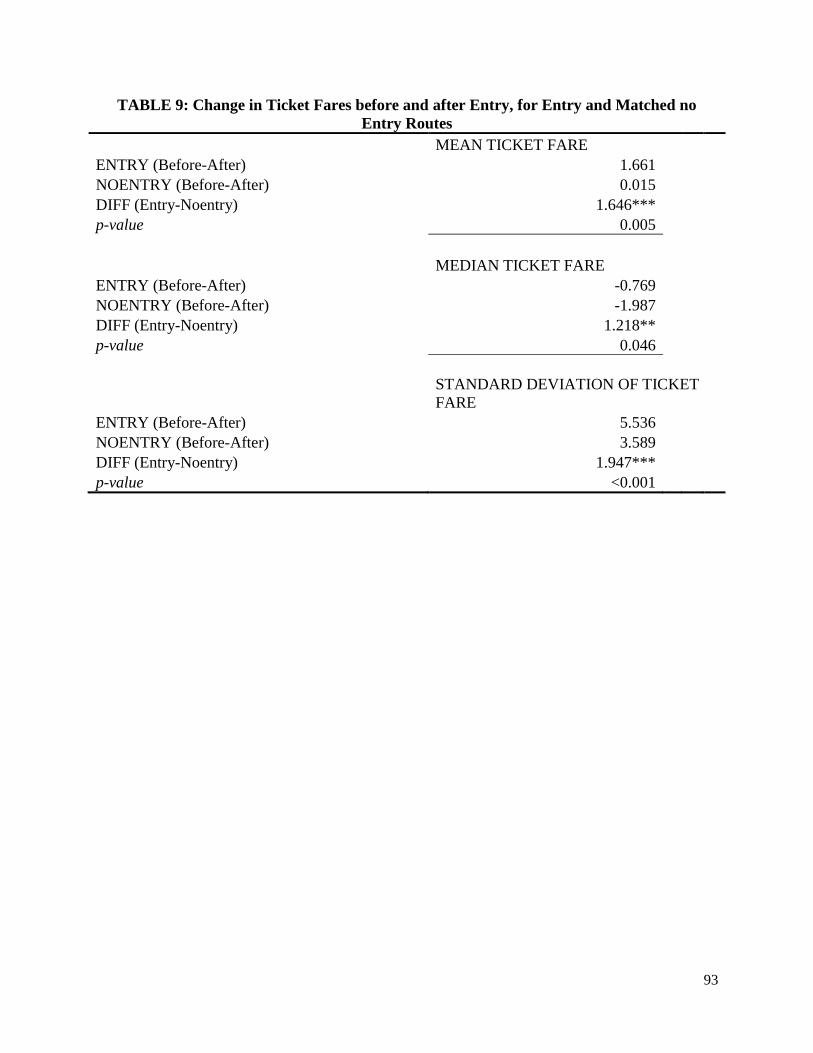
93

TABLE 9: Change in Ticket Fares before and after Entry, for Entry and Matched no

Entry Routes

MEAN TICKET FARE

ENTRY (Before-After) 1.661

NOENTRY (Before-After) 0.015

DIFF (Entry-Noentry) 1.646***

p-value 0.005

MEDIAN TICKET FARE

ENTRY (Before-After) -0.769

NOENTRY (Before-After) -1.987

DIFF (Entry-Noentry) 1.218**

p-value 0.046

STANDARD DEVIATION OF TICKET

FARE

ENTRY (Before-After) 5.536

NOENTRY (Before-After) 3.589

DIFF (Entry-Noentry) 1.947***

p-value <0.001

94

TABLE 10: Entrant-Incumbent-Year Level Analyses: Dependent Variable=% of Entered Market Share

% of Routes Entered % of RSM Entered

% of RSM run by the incumbent Entered

Coef. t-stat

Coef. t-stat

Coef. t-stat

I_AOCIFH

-0.161** -2.12

-0.078** 2.13

-0.026* -1.94

I_SIZE

-0.008 -1.08

-0.007 -0.76

-0.011 -1.17

I_ROA

-0.003 -0.07

-0.006 -0.11

0.074 1.25

I_LEV

0.030 0.51

0.090 1.29

0.024 0.32

I_CFO

0.114 0.91

0.043 0.29

-0.051 -0.32

I_LOSS

0.011 0.47

-0.008 -0.26

0.019 0.64

E_AOCIFH

1.115 1.62

1.343* 1.66

1.643* 1.92

E_SIZE

0.015** 2.06

0.018** 2.04

0.022*** 2.44

E_ROA

0.251** 2.00

0.285* 1.92

0.313** 1.99

E_LEV

-0.064 -0.92

-0.054 -0.66

-0.109 -1.25

E_CFO

0.000 -1.12

0.000 -0.8

-0.001 -1.41

E_LOSS

-0.051** -2.09

-0.067** -2.33

-0.066** -2.2

YEAR FE YES YES YES

N 665 665 665

Adjusted 3.17% 1.02% 4.27%

* Significant at 10%; ** significant at 5%; *** significant at 1%. All tests are two-tailed tests. Variable definitions are provided in Table 1.

95

TABLE 11: Using Alternative Variable of Interest Measure: I_AOCIFH_ASIF

(1) (2)

ENTRY ENTRY

I_AOCIFH_ASIF (-) -13.456** 0.844

(-2.04) (0.10)

I_AOCIFH_ASIF×I_DISCD (-)

-16.946*

(-1.79)

I_DISCD

0.172

(0.61)

I_SIZE 0.041 0.042

(0.44) (0.41)

I_ROA 0.098 0.135

(0.26) (0.36)

I_FUELEXP -0.319 -0.371

(-0.88) (-1.01)

I_CFO 2.677 2.845

(1.26) (1.35)

I_LF 0.613 0.502

(1.13) (0.85)

I_LOSS -0.196 -0.238

(-0.76) (-0.91)

I_LEV 0.836 0.999

(0.82) (0.96)

E_AOCI3 -15.049 -14.514

(-1.09) (-1.08)

E_SIZE 0.176 0.179

(1.17) (1.13)

E_ROA 0.909** 0.879**

(2.30) (2.19)

E_FUELEXP -0.83 -0.855

(-1.24) (-1.34)

E_CFO 2.354 2.170

(0.97) (0.87)

E_LOSS 0.095 0.077

(0.33) (0.26)

E_LEV -0.624 -0.665

(-1.00) (-1.02)

ORIGININCOME 0.000* 0.000*

(1.87) (1.87)

DESTINCOME 0.000 0.000

(0.04) (0.07)

HUB 0.144 0.161

(0.68) (0.73)

96

HHI 3.986*** 3.947***

(7.21) (7.37)

DISTANCE 0.09 0.097*

(1.54) (1.66)

DISTANCE2 -0.003 -0.003

(-1.46) (-1.55)

DENSITY 0.000 0.000

(0.54) (0.31)

DENSITY2 0.000 0.000

(0.36) (0.33)

MEANPOP 0.228* 0.222

(1.73) (1.59)

MKTSIZE -0.065 -0.062

(-0.68) (-0.57)

Constant -10.315 -10.081

(-0.98) (-1.12)

YEAR FE YES YES

Observations 2,825 2,817

Pseudo 16.60% 17.20% Columns 1is based on the regression in model (1), and column 2 is based on the regression in model (2).

The dependent variable is ENTRY in all the four columns. ENTRY=1 if the potential entrant enters the

route in the year following, and zero otherwise. I_AOCIFH_ASIF is the incumbents’ accumulated other

comprehensive income from fuel hedge for the year plus total value of net income from non-designated

fuel hedges. If there are more than one incumbent for the route, I_AOCIFH_ASIF is the weighted average

of AOCIFH for each of the incumbent for the route. I_DISC measures the disclosure level for all the

incumbents from the route by weighting average each incumbent’s disclosure score. I_DISCD is an

indicator variable equal to 1 if the weighted average disclosure score for the route is above the sample

median, and zero otherwise. All other incumbent-variables are the weighted average of each individual

incumbent’s value. Z-statistics with errors clustered by year and route are presented in parentheses. *

Significant at 10%; ** significant at 5%; *** significant at 1%. All tests are two-tailed tests. Variable

definitions are provided in Table 1.

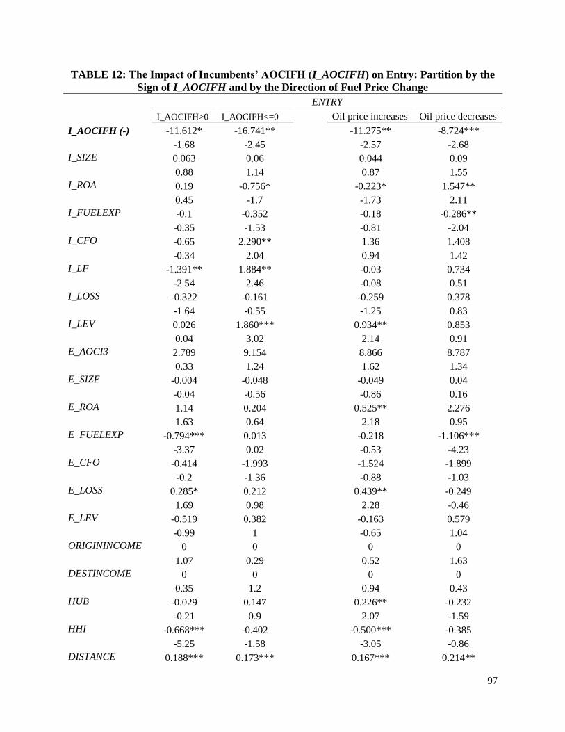
97

TABLE 12: The Impact of Incumbents’ AOCIFH (I_AOCIFH) on Entry: Partition by the

Sign of I_AOCIFH and by the Direction of Fuel Price Change

ENTRY

I_AOCIFH>0 I_AOCIFH<=0

Oil price increases Oil price decreases

I_AOCIFH (-) -11.612* -16.741**

-11.275** -8.724***

-1.68 -2.45

-2.57 -2.68

I_SIZE 0.063 0.06

0.044 0.09

0.88 1.14

0.87 1.55

I_ROA 0.19 -0.756*

-0.223* 1.547**

0.45 -1.7

-1.73 2.11

I_FUELEXP -0.1 -0.352

-0.18 -0.286**

-0.35 -1.53

-0.81 -2.04

I_CFO -0.65 2.290**

1.36 1.408

-0.34 2.04

0.94 1.42

I_LF -1.391** 1.884**

-0.03 0.734

-2.54 2.46

-0.08 0.51

I_LOSS -0.322 -0.161

-0.259 0.378

-1.64 -0.55

-1.25 0.83

I_LEV 0.026 1.860***

0.934** 0.853

0.04 3.02

2.14 0.91

E_AOCI3 2.789 9.154

8.866 8.787

0.33 1.24

1.62 1.34

E_SIZE -0.004 -0.048

-0.049 0.04

-0.04 -0.56

-0.86 0.16

E_ROA 1.14 0.204

0.525** 2.276

1.63 0.64

2.18 0.95

E_FUELEXP -0.794*** 0.013

-0.218 -1.106***

-3.37 0.02

-0.53 -4.23

E_CFO -0.414 -1.993

-1.524 -1.899

-0.2 -1.36

-0.88 -1.03

E_LOSS 0.285* 0.212

0.439** -0.249

1.69 0.98

2.28 -0.46

E_LEV -0.519 0.382

-0.163 0.579

-0.99 1

-0.65 1.04

ORIGININCOME 0 0

0 0

1.07 0.29

0.52 1.63

DESTINCOME 0 0

0 0

0.35 1.2

0.94 0.43

HUB -0.029 0.147

0.226** -0.232

-0.21 0.9

2.07 -1.59

HHI -0.668*** -0.402

-0.500*** -0.385

-5.25 -1.58

-3.05 -0.86

DISTANCE 0.188*** 0.173***

0.167*** 0.214**

98

2.89 3.41

4.56 2.2

DISTANCE2 -0.006*** -0.005***

-0.005*** -0.007**

-2.7 -3.59

-4.57 -2.26

DENSITY 0.000 0.000

0.000 0.000

0.61 0.48

0.43 0.81

DENSITY2 0.000 0.000

0.000 0.000

0.52 0.91

0.08 0.61

MEANPOP 0.176** 0.084

0.131* 0.01

2.02 0.85

1.85 0.08

MKTSIZE 0.059 0.075

0.13 -0.047

0.54 0.61

1.01 -0.25

Constant -6.674 -6.019**

-5.339*** -1.766

-1.12 -2.24

-3.47 -0.68

YEAR FE YES YES

YES YES

Observations 1,204 1,613

1,997 820

Pseudo 13.54% 18.24% 13.46% 13.75%

This table presents the results based on the regression in model (1). The dependent variable is ENTRY for

all four columns. Column 1 presents results using the positive I_AOCIFH sample and column 2 presents

results for the non-positive I_AOCIFH sample. Column 3 focuses on years when oil price increases and

Column 4 on years when oil price decreases. ENTRY=1 if the potential entrant enters the route in the year

following, and zero otherwise. Z-statistics clustered by year and route are presented in parentheses. *

Significant at 10%; ** significant at 5%; *** significant at 1%. All tests are two-tailed tests. Variable

definitions are provided in Table 1.

99

TABLE 13: The Impact of Incumbents’ AOCIFH (I_AOCIFH) and its Interaction with

Disclosure on Entry: Probit Regressions Using One-airport Present Carriers as Entrants

(1) (2) (3) (4)

ENTRY ENTRY ENTRY ENTRY

I_AOCIFH (-) -8.925*** -11.563*** -11.168*** -1.679

(-3.21) (-3.63) (-3.25) (-0.19)

I_AOCIFH×I_DISCD (-)

-17.863***

(-2.96)

I_DISCD

0.49

(1.18)

I_SIZE

-0.008 0.004 -0.08

(-0.14) (0.06) (-0.76)

I_ROA

-0.262 -0.314 -0.063

(-0.7) (-0.73) (-0.10)

I_FUELEXP

-0.06 -0.067 0.229

(-0.36) (-0.43) (0.84)

I_CFO

1.652** 1.520** 2.017

(2.22) (2.14) (0.96)

I_LF

0.281 0.274 0.62

(1.14) (1.09) (0.80)

I_LOSS

0.139 0.087 -0.311

(1.12) (0.60) (-1.01)

I_LEV

0.238 0.093 -1.306

(0.68) (0.23) (-1.26)

E_AOCI3

4.072 -2.591

(0.73) (-0.32)

E_SIZE

0.055 -0.164

(0.95) (-0.78)

E_ROA

0.195 0.386

(0.33) (0.41)

E_FUELEXP

0.128 -0.404

(0.44) (-0.49)

E_CFO

-3.000*** -3.495***

(-3.35) -2.74

E_LOSS

-0.117 -0.148

(-0.72) -0.55

E_LEV

-0.906*** -1.819***

(-3.22) -4.19

ORIGININCOME 0.000 0.000 0.000 0.000

0.71 0.71 (0.67) 0.28

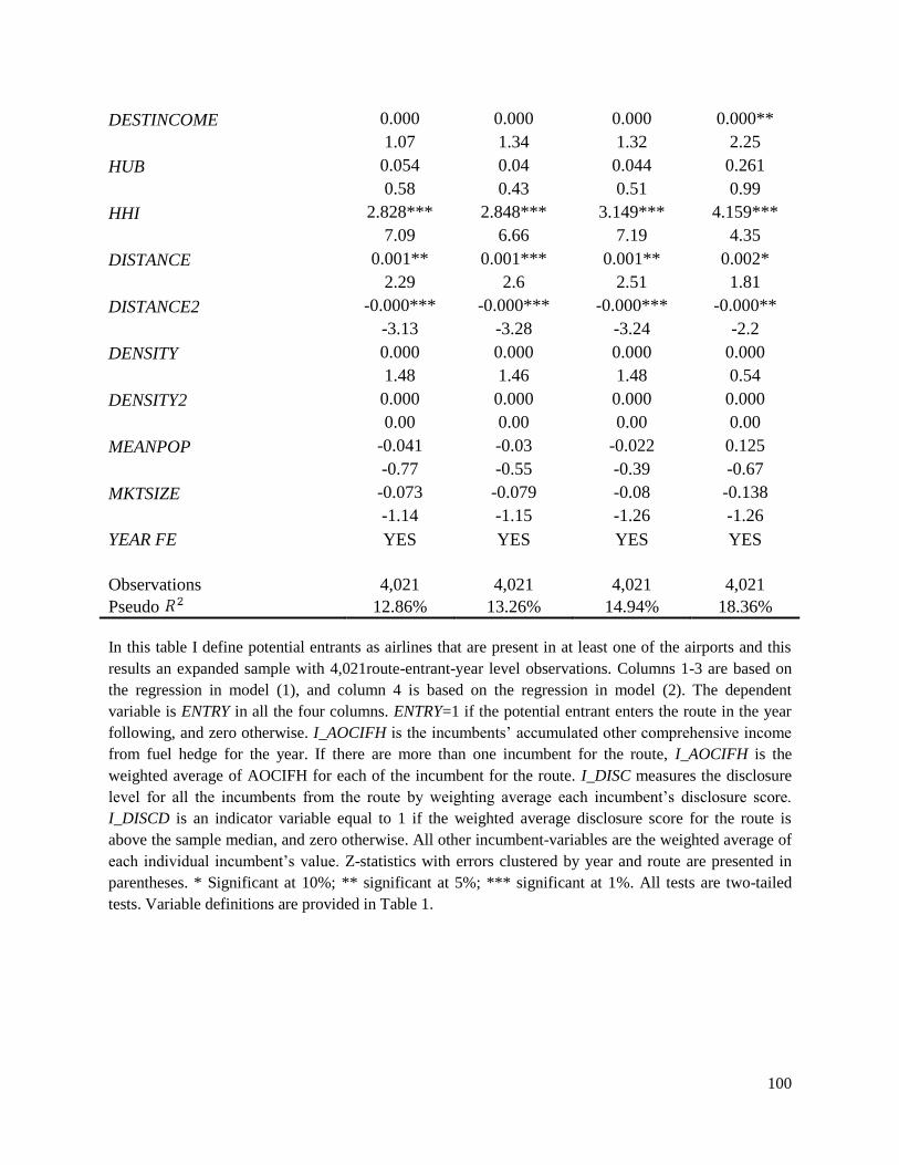
100

DESTINCOME 0.000 0.000 0.000 0.000**

1.07 1.34 1.32 2.25

HUB 0.054 0.04 0.044 0.261

0.58 0.43 0.51 0.99

HHI 2.828*** 2.848*** 3.149*** 4.159***

7.09 6.66 7.19 4.35

DISTANCE 0.001** 0.001*** 0.001** 0.002*

2.29 2.6 2.51 1.81

DISTANCE2 -0.000*** -0.000*** -0.000*** -0.000**

-3.13 -3.28 -3.24 -2.2

DENSITY 0.000 0.000 0.000 0.000

1.48 1.46 1.48 0.54

DENSITY2 0.000 0.000 0.000 0.000

0.00 0.00 0.00 0.00

MEANPOP -0.041 -0.03 -0.022 0.125

-0.77 -0.55 -0.39 -0.67

MKTSIZE -0.073 -0.079 -0.08 -0.138

-1.14 -1.15 -1.26 -1.26

YEAR FE YES YES YES YES

Observations 4,021 4,021 4,021 4,021

Pseudo 12.86% 13.26% 14.94% 18.36%

In this table I define potential entrants as airlines that are present in at least one of the airports and this

results an expanded sample with 4,021route-entrant-year level observations. Columns 1-3 are based on

the regression in model (1), and column 4 is based on the regression in model (2). The dependent

variable is ENTRY in all the four columns. ENTRY=1 if the potential entrant enters the route in the year

following, and zero otherwise. I_AOCIFH is the incumbents’ accumulated other comprehensive income

from fuel hedge for the year. If there are more than one incumbent for the route, I_AOCIFH is the

weighted average of AOCIFH for each of the incumbent for the route. I_DISC measures the disclosure

level for all the incumbents from the route by weighting average each incumbent’s disclosure score.

I_DISCD is an indicator variable equal to 1 if the weighted average disclosure score for the route is

above the sample median, and zero otherwise. All other incumbent-variables are the weighted average of

each individual incumbent’s value. Z-statistics with errors clustered by year and route are presented in

parentheses. * Significant at 10%; ** significant at 5%; *** significant at 1%. All tests are two-tailed

tests. Variable definitions are provided in Table 1.

101

TABLE 14: Variables Definition—Chapter 2

Firm Characteristics

DISC Risk management disclosure score based on the 13 items in

Appendix B. For each of the 13 items, if disclosed, an indicator

variable takes the value of 1, and zero otherwise. DISC takes the

average value of the 13 indicator variables, averaged for 2005-

2008.

SCOPE Percentage of expected fuel consumption in the 12 month that is

being hedged averaged for 2005-2008.

AOCI_RAW Accumulated other comprehensive income from fuel hedge (in

millions) averaged for 2005-2008.

ROA Net income scaled by total assets averaged for 2005-2008.

AOCIFH Accumulated other comprehensive income from fuel hedge

divided by total assets, averaged for 2005-2008.

LOWCOST Indicator variable, taking the value of 1 if the airline is a low-cost

carrier, and zero otherwise.

Event Indicators

D1 Indicator variable, =1 for the three-day window around Event 1,

and 0 otherwise.

D2 Indicator variable, =1 for the three-day window around Events 2-5,

and 0 otherwise. D3 Indicator variable, =1 for the three-day window around Event 6,

and 0 otherwise. D4 Indicator variable, =1 for the three-day window around Events 7-

10, and 0 otherwise. D5 Indicator variable, =1 for the three-day window around Event 11,

and 0 otherwise. D6 Indicator variable, =1 for the three-day window around Event 12,

and 0 otherwise. D7 Indicator variable, =1 for the three-day window around Event 13,

and 0 otherwise.

102

TABLE 15: Descriptive Statistics and Correlations (2005-2008 average)

Panel A: Descriptive Statistics

Variable Mean Median Std Dev P5 P25 P75 P95

DISC 0.756 0.780 0.089 0.533 0.716 0.833 0.838

AOCI_RAW (Million) -37.117 -0.500 233.699 -631.000 -57.375 0.000 437.500

AOCIFH -0.057% -0.024% 1.003% -1.395% -0.510% 0.000% 2.819%

SCOPE (%) 25.117 21.750 16.771 4.067 13.875 35.125 61.250

LOWCOST 0.417 0.000 0.515 0.000 0.000 1.000 1.000

ROA -0.004 -0.005 0.047 -0.074 -0.025 0.018 0.085

Panel B: Correlations

DISCLOSE SCOPE AOCIFH LOWCOST

SCOPE 0.521

AOCIFH 0.032 0.489

LOWCOST -0.403 -0.114 0.491

ROA 0.157 -0.152 0.391 0.229

Please see Table 14 for variables definition. My sample consists of 41 U.S. airline-year observations with available return and accounting

information for the period 2005-2008. For each variable, I take the average value for 2005-2008 and provide descriptive statistics, following

Beatty et al. (1996) and Dou et al. (2013).

103

TABLE 16: Average Stock Returns around Event Dates during the Deliberation of SFAS

161: U.S. Airline Industry

Event Indicator Mean return

D1

-0.008

(-0.62)

D2

0.006

(0.46)

D3

0.008

(0.63)

D4

-0.018*

(-1.72)

D5

0.012

(0.94)

D6

0.039***

(3.04)

D7

0.028**

(2.21)

Mean 0.013**

(2.19)

The table reports mean stock price reaction (t-statistics) of a portfolio of the sample firms around key

event dates during the deliberation of SFAS 161 (with t-statistics in the parentheses). The stock price

reactions are estimated using an augmented market model over the period from January 1, 2005 to

December 31, 2008. Daily portfolio returns are computed by value weighting the daily returns of the

sample firms. Events 1-13 are listed in Appendix A and D1-D7 are defined in Table 14. ***, **, and *

denote statistical significance at the 1%, 5%, and 10% levels, respectively.

104

TABLE 17: Sefcik and Thompson (1986) Cross-sectional Analyses of Stock Price Reactions

around Key Events: 1 Indicator

(1) (2) (3) (4)

DISC 0.097** 0.029 0.153** 0.085*

(1.97) (0.34) (2.00) (1.95)

SCOPE

-0.001** -0.001** -0.001*** -0.001*

(-2.25) (-1.97) (-2.87) (-1.72)

LOWCOST

-0.025**

(-2.04)

ROA

-0.322***

(-2.89)

AOCIFH

-0.345

(-1.54) This table reports the Sefcik and Thompson (1986) portfolio time-series regression results for my sample

firms (with t-statistics in the parentheses). Key events are listed in Appendix A. In this table, one event

indicator is assigned to all the 13 events. ***, **, and * denote statistical significance at the 1%, 5%, and

10% levels, respectively.

105

TABLE 18: Sefcik and Thompson (1986) Cross-sectional Analyses of Stock Price Reactions

around Key Events: 7 Indicators

D1 D2 D3 D4 D5 D6 D7

Panel A

DISC -0.038 -0.016 0.138 0.007 -0.075 0.185** 0.098*

(-0.42) (-0.18) (1.52) (0.08) (-0.82) (2.03) (1.78)

SCOPE

0.000 0.000 0.000* 0.000 0.000 -0.001*** -0.001**

(0.16) (-1.03) (-1.68) (0.15) (-0.04) (-3.51) (-2.28)

Panel B

DISC -0.063 -0.04 0.148* 0.066 -0.066 0.153* 0.03

(-0.73) (-0.47) (1.71) (0.76) (-0.76) (1.772) (0.35)

SCOPE

0.000 0.000 0.000 0.000 0.000 -0.001*** -0.001**

(0.29) (-0.94) (-1.58) (-0.16) (-0.09) (-3.451) (-1.99)

LOWCOST -0.009 -0.009 0.004 0.022* 0.003 -0.011 -0.025**

(-0.73) (-0.73) (0.30) (1.77) (0.26) (-0.942) (-2.05)

Panel C

DISC -0.034 0.006 0.139* -0.041 -0.081 0.164* 0.154*

(-0.36) (0.06) (1.86) (-0.43) (-0.85) (1.711) (1.91)

SCOPE

0.000 0.000 0.000 0.000 0.000 -0.001*** -0.001***

(0.07) (-1.26) (-1.32) (0.89) (0.07) (-2.763) (-2.89)

ROA

-0.023 -0.126 -0.005 0.276*** 0.038 0.123 -0.321***

(-0.21) (-1.13) (-0.04) (2.48) (0.34) (1.103) (-2.89)

Panel D

DISC -0.046 -0.03 0.151* 0.039 -0.071 0.186** 0.086

(-0.515) (-0.337) (1.680) (0.433) (-0.785) (2.071) (0.958)

SCOPE

0.000 0.000 -0.001* 0.000 0.000 -0.001*** -0.001*

(0.414) (-0.433) (-1.779) (-0.972) (-0.171) (-3.219) (-1.664)

AOCIFH

-0.229 -0.414 0.372 0.921** 0.112 0.045 -0.344

(-0.489) (-0.887) (0.797) (1.971) (0.24) (0.097) (-0.736)

This table reports the Sefcik and Thompson (1986) portfolio time-series regression results for my sample

firms (with t-statistics in the parentheses). Key events are listed in Appendix A and indicators are defined

in Table 14. In this table, seven event indicators are assigned to all the 13 events. ***, **, and * denote

statistical significance at the 1%, 5%, and 10% levels, respectively.

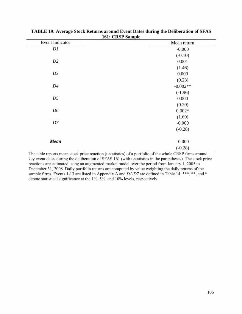
106

TABLE 19: Average Stock Returns around Event Dates during the Deliberation of SFAS

161: CRSP Sample

Event Indicator Mean return

D1

-0.000

(-0.10)

D2

0.001

(1.46)

D3

0.000

(0.23)

D4

-0.002**

(-1.96)

D5

0.000

(0.20)

D6

0.002*

(1.69)

D7

-0.000

(-0.28)

Mean -0.000

(-0.28)

The table reports mean stock price reaction (t-statistics) of a portfolio of the whole CRSP firms around

key event dates during the deliberation of SFAS 161 (with t-statistics in the parentheses). The stock price

reactions are estimated using an augmented market model over the period from January 1, 2005 to

December 31, 2008. Daily portfolio returns are computed by value weighting the daily returns of the

sample firms. Events 1-13 are listed in Appendix A and D1-D7 are defined in Table 14. ***, **, and *

denote statistical significance at the 1%, 5%, and 10% levels, respectively.