Strangely Dispersed Minimal Sets in the Quasiperiodically ...

Strangely Dispersed Minimal Sets in theQuasiperiodically Forced Arnold Circle Map

Glendinning, P. A. and Jäger, T. and Stark, J

2008

MIMS EPrint: 2008.103

Manchester Institute for Mathematical SciencesSchool of Mathematics

The University of Manchester

Reports available from: http://eprints.maths.manchester.ac.uk/And by contacting: The MIMS Secretary

School of Mathematics

The University of Manchester

Manchester, M13 9PL, UK

ISSN 1749-9097

http://eprints.maths.manchester.ac.uk/

Strangely Dispersed Minimal Sets in the

Quasiperiodically Forced Arnold Circle Map

P.A. Glendinning∗, T. Jager†and J. Stark‡

July 29, 2008

Abstract

We study quasiperiodically forced circle endomorphisms, homotopic to the identity, andshow that under suitable conditions these exhibit uncountably many minimal sets with acomplicated structure, to which we refer to as ‘strangely dispersed’. Along the way, wegeneralise some well-known results about circle endomorphisms to the uniquely ergodicallyforced case. Namely, all rotation numbers in the rotation interval of a uniquely ergodicallyforced circle endomorphism are realised on minimal sets, and if the rotation interval hasnon-empty interior then the topological entropy is strictly positive. The results apply inparticular to the quasiperiodically forced Arnold circle map, which serves as a paradigmexample.

1 Introduction

Quasiperiodically forced circle (QPF) maps such as the QPF forced Arnold map f : T1 ×T1 → T1 × T1

(1.1) f(θ, ϕ) =“

θ + ω, ϕ + τ +α

2πsin(2πϕ) + β sin(2πθ) mod 1

”

,

where T1 = R/Z denotes the circle and ω /∈ Q, have been studied by a number of authors.The motivation for this comes from two related directions. First, Grebogi et al [1] showedthat it is possible to have strange (i.e. geometrically complicated) nonchaotic attractors(SNAs) over a range of parameter values with positive measure, and later (e.g. [2, 3, 4, 5])that maps such as 1.1 are good candidates for simple invertible examples of such behaviour.This aspect has been followed up in the work of Feudel and Pikovsky and ourselves amongstothers [6, 7, 8, 9]. Secondly, from a different perspective Herman [10] had already provedthe existence of SNA in certain parameter families of QPF circle diffeomorphisms that areinduced by the projective action of SL(2, R)-cocycles over an irrational rotation.

Despite considerable interest over subsequent years, rigourous mathematical results re-mained rare. The original Grebogi et al example [1] was a non-invertible map with aspecial structure. This structure was abstracted by Keller, who proved the existence ofSNAs under simple conditions in this class of maps [11]. Jager [12] further analysed thestructure of such invariant sets. Subsequently, Glendinning et al [13] proved that althoughnon-chaotic in the sense of Lyapunov exponents, such systems did exhibit sensitive depen-dence on initial conditions. Meanwhile, Stark [14] showed that SNAs in QPF maps couldnot be non-smooth graphs, but had to have a more complex structure, and an extension ofthis approach by Sturman and Stark [15] showed that the normal Lyapunov exponents ofa SNA could not all be negative. Finally, new methods were established quite recently byBjerklov and Jager, which allow to prove the existence of SNA in much broader classes ofquasiperiodically forced maps than the two mentioned above [16, 17, 18].

∗University of Manchester. Email: [email protected]†College de France, Paris. Email: [email protected]‡Imperial College London. Email: [email protected]

1

2 T. Jager, P.A. Glendinning and J. Stark

Additional properties of invertible circle maps were derived in [19, 20], and used to-gether with results in [21] to give a generalization of the Poincare classification of circlehomeomorphisms [22]. Further, Jager and Keller [21] showed that if a QPF circle homeo-morphism, homotopic to the identity, with appropriate conditions on its rotation number,was topologically transitive then any minimal set was ‘strangely dispersed’ (see below fordefinition). Dynamics of this type are constructed in [23]. However, it is also known thatthe minimal set is unique in this situation ([24] or [23]), such that there is no co-existenceas in Theorem 2.6. Further, the examples given in [23] only have low regularity, and it isstill completely open whether the same phenomenon can occur in smooth systems as well(e.g. in QPF analytic circle diffeomorphisms).

Here we turn to examine the behaviour of QPF maps such as the forced Arnold map(1.1) above. This is motivated both by the considerable volume of numerical work, and thefact that the unforced Arnold map has a rich and interesting structure has been described insome detail by MacKay and Tresser [25]. This gave a beautiful description of the transitionto chaotic behaviour in the unforced case. Numerical experiments have suggested that in theQPF map the appearance of strange nonchaotic structures occurs at the complex boundarybetween the regular and chaotic parameter regions.

Unfortunately, MacKay and Tresser’s analysis made heavy use of periodic orbits anddoubling cascades. Since (1.1) has no periodic orbits (this follows immediately from thefact that ω is irrational) it is not immediately clear how to generalize their work to theQPF case. Indeed, almost all of our understanding of chaos is based on generalizations ofthe horseshoe (e.g. [26]) and horseshoes imply the existence of periodic orbits, so eitherhorseshoes are irrelevant for the study of chaos in quasiperiodically forced systems or thechaos is essentially a suspension of a horseshoe. If the former is the case then it is naturalto ask which orbits form the backbone of the chaos, i.e. which orbits play the role of theperiodic orbits in the horseshoe? There are therefore at least three reasons for consideringnoninvertible quasiperiodically forced circle maps, k > 1 in (1.1). First in an attemptto obtain some rigorous results on complex invariant sets, second as an extension of theresults for noninvertible circle maps, and third as a move towards understanding chaoticsets which are not modelled by horseshoes. Our main motivation has been the first ofthese. We shall prove that if k and β are sufficiently large then the the forced Arnold map(1.1) exhibits uncountably many minimal sets with a complicated structure, to which werefer to as ‘strangely dispersed’. In the proof of this result it becomes necessary to proveanalogues of a number of results for noninvertible circle maps in the context of noninvertiblequasiperiodically forced circle maps. An appealing, albeit heuristic, interpretation of thisresult is that in moving along a path in parameter space from a nonchaotic state of aninvertible quasiperiodically forced circle map to a chaotic noninvertible circle map of thetype discussed below it is necessary to create strange nonchaotic invariant sets. One wayof achieving this is to create this set as a stable set, which later loses stability. If this isthe case then it goes some way towards explaining why nonchaotic strange attractors mustexist in such families.

Acknowledgements. We would like to thank Sylvain Crovisier for pointing out to usthe result by Bowen [27] and its consequences for the entropy of QPF monotone circle maps.Tobias Jager was supported by a research fellowship of the German Research Foundation(DFG, Ja 1721/1-1).

2 Main Results

Let T1 = R/Z denote the circle and suppose Θ is a compact metric space and r : Θ → Θa continuous map. We consider skew-products on Θ × T1 given by continuous maps f :Θ × T1 → Θ × T1 of the form

(2.1) f(θ, ϕ) = (r(θ), fθ(ϕ)) .

The case we are primarily interested in is that of QPF circle endomorphisms, that is Θ = T1

and r(θ) = θ + ω with ω ∈ T1 irrational. However, some of the results we obtain naturally

Strangely Dispersed Minimal Sets . . . 3

generalise to the uniquely ergodically forced (UEF) case (meaning that there exists a uniquer-invariant probability measure µ on Θ).

The maps fθ in (2.1) will be called fibre maps. Most of the time, we will assume inaddition that f is homotopic to the map (θ, ϕ) 7→ (r(θ), ϕ). If this holds, we say f ishomotopic to the identity (slightly abusing terminology in the case that r is not homotopicto the identity on Θ). Then all fθ are circle endomorphisms of degree one, and furtherthere exist a continuous lift F : Θ × R → Θ × R that satisfies π ◦ F = f ◦ π, whereπ : Θ × R → Θ × T1 denotes the natural projection. Moreover, if Θ is connected, thenthese lifts are always uniquely defined modulo an integer. In the same way we can definethe continuous lifts Fθ : R → R of fibre maps fθ which satisfy π ◦ Fθ = fθ ◦ π, whereπ : R → T1 denotes the natural projection, with the obvious abuse of notation on theprojection operators π.

We define the fibred rotation interval of a lift F by

(2.2) ρfib(F ) :=

lim supn→∞

1

n(F n

θ (x) − x)

˛

˛

˛

˛

(θ, x) ∈ Θ × R

ff

.

where F nθ (x) = Frn−1(θ) ◦ . . . ◦ Fθ(x). Observe that ρfib for two different lifts of the same

UEF endomorphism of Θ × T1 will differ by an integer translation.An important special case will be the one of UEF (or QPF) monotone circle maps,

by which we mean that each fibre map fθ preserves the cyclic order on T1 (but we allowf to be non-injective). This is true if and only if the fibre maps Fθ of any lift F of fare monotonically increasing. It is a well-known result of Herman [10] that the fibredrotation interval of a UEF monotone circle map is always a single point (restated below asTheorem 3.3).

Remark 2.1. Note that in the QPF case there are in general several ways of assigninga rotation set to a torus endomorphism which is homotopic to the identity, as discussedvery concisely in [28]. However, if f has skew-product structure as in (2.1), then all thesedifferent notions coincide. This follows easily from Theorem 2.2 below, in combinationwith [28, Theorem 2.4 and Corollary 2.6]. The above definition is the one which is mostconvenient for our purposes, and we have adapted it to the fibred setting by projecting tothe second coordinate, thus obtaining a subset of the real line instead of a subset of R2 fora general endomorphism of T2.

Recall that a closed, f -invariant set M is minimal if it contains no proper f -invariantclosed subset [26]. This is equivalent to the orbit of every point in M being dense in M .The topological entropy htop(f) of a map f is a common measure of the complexity of itsdynamics, and indeed provides one of the standard definitions of chaotic behaviour [26]. Adefinition and brief overview is given below in Section 4. The following theorem is then ageneralisation of well-known results on unforced circle endomorphisms (see, for example,[29]).

Theorem 2.2. Suppose F is the lift of a UEF circle endomorphism f : Θ×T1 → Θ×T1,homotopic to the identity. Then ρfib(F ) is a closed interval (including the possibility of asingleton ρfib(F ) = [ρ, ρ]). For any ρ ∈ ρfib(F ) there exists a minimal set Mρ ⊂ Θ × T1

with the following properties:

(i) 1n(F n

θ (x) − x) converges uniformly to ρ on π−1(Mρ) as n → ∞.

(ii) htop(f |Mρ) = 0.

The proof of (i) is given in Section 3 and that of (ii) at the end of Section 4. Although thedynamics on each Mρ is simple, if the rotation interval is non-trivial, the overall dynamicsof the map is complex:

Theorem 2.3. Suppose f is a UEF circle endomorphism, homotopic to the identity, withlift F . If ρfib(F ) has non-empty interior, then htop(f) > 0.

The proof is given in Section 4. We remark that for a QPF monotone circle map f thesituation is quite different. As mentioned above, the rotation interval is reduced to a singlepoint in this case, and the topological entropy is always zero. The latter is a more or lessdirect consequence of a result by Bowen [27], see Section 4 below.


Once these basic facts are established, we can turn to a new phenomenon which is spe-cific to the quasiperiodically forced setting. In the case of unforced circle endomorphisms,minimal sets may be either periodic orbits or Cantor sets, corresponding to rational andirrational rotation numbers, respectively. In the quasiperiodically forced case however, theycan have a much more complicated structure. In order to make this precise, we introducethe following notion.

Definition 2.4. Suppose f is a QPF circle endomorphism, homotopic to the identity. Wesay a compact subset M ⊆ T2 is a strangely dispersed minimal set, if it has the followingthree properties:

(i) M is a minimal set.

(ii) Every connected component C of M is contained in a single fibre, that is π1(C) is asingleton.

(iii) For any point (θ, x) ∈ M and any open neighbourhood U of (θ, x), the set π1(U ∩M)contains a non-empty open interval.

Remark 2.5.

(a) Property (iii) is a rather direct consequence of (i) (see Section 5). We have onlyincluded it here to emphasize the peculiarity of property (ii).

(b) It is actually not difficult to construct a set which has properties (ii) and (iii). Indeed,let (aη)η∈T1∩Q be any sequence of strictly positive real numbers with

P

η∈T1∩Qaη = 1.

For any θ ∈ T1, let φ(θ) :=P

η∈[0,θ]∩Qaη. Then the topological closure of the graph

Φ := {(θ, φ(θ)) | θ ∈ T1} of φ is a compact set that has these two properties. Ofcourse, the interesting point in the above definition is to have a set with this structureas the minimal set of a dynamical system.

It will follow from our arguments in Section 5 that the appearance of strangely dispersedminimal sets is a rather general phenomenon for QPF circle endomorphisms, provided thatthe quasiperiodic forcing has a certain strength. However, for simplicity we will formulatethe results only for a particular example, namely for the QPF Arnold Circle Map (1.1).

Theorem 2.6. Suppose f is given by (1.1), with driving frequency ω ∈ T1 \ Q and realparameters τ, α and β.

(a) If α > 1 and |β| ≥ 32, then for any ρ ∈ ρfib(f) there exists a strangely dispersed

minimal set Mρ which satisfies properties (i) and (ii) in Theorem 2.2 .

(b) If |α| ≥ 52π, then ρfib(f) has length ≥ 1, in particular its interior is non-empty.

Remark 2.7.

(a) The bounds given here are not optimal and may surely be improved by a more carefulanalysis. Further, part (b) of this theorem is rather trivial, but it is important forthe interpretation of (a). Namely, if both conditions in (a) and (b) are satisfiedsimultaneously, we obtain the existence of uncountably many pairwise disjoint andstrangely dispersed minimal sets, one for each rotation number in the rotation interval.Albeit most likely superficial, this presents an intriguing analogy to the theory of twistmaps, where at suitable parameter values the standard map exhibits uncountably manyAubry-Mather sets, again one for each rotation number in the rotation interval.

(b) As indicated in the introduction above, the existence of strangely dispersed minimalsets is already known in QPF circle homeomorphisms [21, 23, 24] though existingconstructions only work in maps of low regularity.

3 Plateau Maps and Rotation Numbers: Proof of

Theorem 2.2

In order to prove Theorem 2.2, we will first be concerned with unforced circle endomor-phisms and their lifts. The basic idea, which is the use of plateau maps to identify orbits


with a given rotation number, was first introduced by Boyland [30] (see also [29] for asurvey). Let E denote the space of continuous maps G : R → R which are the lift of a circleendomorphism of degree one. The latter just amounts to saying that

(3.1) G(x + k) = G(x) + k ∀k ∈ Z .

We equip E with the topology of uniform convergence. Further, we denote by Emon thespace of all maps in G ∈ E which are monotonically increasing. Then G ∈ Emon if andonly if it is the lift of a monotone circle map of degree one. Note that we explicitly allowfor G ∈ Emon to be non-injective, in which case there exist intervals that are mapped toa single point by G. We refer to such intervals as plateaus, and call maps in Emon plateaumaps (including the case when there are no plateaus, for simplicity).

For any G ∈ Emon, let U(G) denote the union of the interiors of all plateaus of G. Inother words

U(G) = {x ∈ R | ∃ε > 0 : G([x − ε, x + ε]) = {G(x)}} .

Now suppose G ∈ E . We assign to G a pair of plateau maps G− ≤ G ≤ G+ (Figure 1) by

G+(x) := supξ≤x

G(ξ) and G−(x) := infξ≥x

G(ξ) .

Figure 1: Illustration of the plateau maps G+ and G− and the functions Φt and Gt.

Note that if G is a plateau map itself, then G− = G+ = G. Further, it follows easilyfrom (3.1) that

(3.2) G+(x) = supξ∈[x−1,x]

and G−(x) = infξ∈[x,x+1]

G(ξ) .

The reason why plateau maps are such a convenient tool for the computation of rotationintervals is the fact that they always have a uniquely defined rotation number, and thisremains true in the quasiperiodically forced setting (see Theorem 3.3 below). Furthermore,as the following proposition shows, there always exists a homotopy between the maps G−

and G+ with some additional nice properties, and this will be the key ingredient in theproof of Theorem 2.2 .

Proposition 3.1. There exists a continuous mapping R×[0, 1]×E → R, (x, t, G) 7→ Gt(x),with the following properties:

(i) The family (Gt)t∈[0,1] is a homotopy between G− and G+, that is G0 = G− andG1 = G+.

(ii) For all t ∈ [0, 1] we have Gt ∈ Emon.


(iii) For all x ∈ R the map t 7→ Gt(x) is monotonically increasing.

(iv) If Gt(x) 6= G(x), then x ∈ U(Gt).

Note that due to the periodicity property (3.1) of G ∈ E and compactness, the inducedmapping [0, 1] × E → Emon, (t, G) 7→ Gt is continuous as well.

Proof. The mappings R × E → R, (x, G) 7→ G±(x) are clearly continuous and monotonein x. They are also continuous and monotonically increasing in G, the latter with respectto the partial ordering on E given by G1 ≤ G2 if G1(x) ≤ G2(x) ∀x ∈ R. Similarly, themapping (Figure 1)

(3.3) Φ : R × [0, 1] × E → R , (x, t, G) 7→ Φt(x) := supξ∈[x−t,x]

G(ξ) ,

is continuous and monotonically increasing t and G. We define our required homotopy by

(3.4) Gt(x) := (Φt)−(x) = inf

ζ≥xsup

ξ∈[ζ−t,ζ]

G(ξ) .

For any given x ∈ E the function (x, t) 7→ Gt(x) is continuous as the composition ofcontinuous functions. By definition Φ0 = G, and hence G0 = G−. Also, by (3.2) we haveΦ1 = G+ and hence G1 = (G+)− = G+. This proves (i). For any t ∈ [0, 1] the mapGt = (Φt)

− is a plateau map, since it is in the image of the mapping E → Emon, G 7→ G−.Thus (ii) holds. The monotonicity of the mapping Φ in t and of the mapping G 7→ G− inG immediately implies (iii).

It remains to prove (iv). We first show that if for a given t ∈ [0, 1] and x ∈ R we haveGt(x) < Φt(x) then Gt is constant in an open neighbourhood of x. Since Gt = (Φt)

−,and Φt is continuous, then if Gt(x) < Φt(x) there must exist some ξ0 > x with Φt(ξ0) =Gt(x). By the continuity of Φt we further have Φt(x

′) > Gt(x) for all x′ in a small openneighbourhood U of x. Without loss of generality, we shrink U so that it does not contain ξ0,which implies that x′ < ξ0 for all x′ ∈ U . This means that infξ≥x′ Φt(ξ) ≤ Φt(ξ0) for all x′ ∈U . If x′ ≥ x, then automatically infξ≥x′ Φt(ξ) ≥ infξ≥x Φt(ξ) = Φt(ξ0), whereas if x′ < x,then infξ≥x′ Φt(ξ) = min{infx′≤ξ<x Φt(ξ), infξ≥x Φt(ξ)} = min{infx′≤ξ<x Φt(ξ), Φt(ξ0)} =Φt(ξ0), since Φt(ξ) > Gt(x) = Φt(ξ0) for all ξ ∈ U . Hence Gt(x

′) = Φt(ξ0) for all x′ ∈ U ,so that Gt is constant on U as required.

To now prove (iv), fix t ∈ [0, 1] and x ∈ R with Gt(x) 6= G(x). First suppose Gt(x) <G(x) (Figure 2a). Since G(x) ≤ Φt(x) for all x ∈ R, this implies that Gt(x) < Φt(x) andhence by the above Gt is constant on an open neighbourhood of x, as required.

On the other hand, if Gt(x) > G(x), we consider two cases. By definition, we alwayshave Gt(x) ≤ Φt(x). Hence either Gt(x) < Φt(x) (Figure 2b) or Gt(x) = Φt(x). In theformer case we again apply the argument above.

In the latter case, Gt(x) = Φt(x), the definition of Φt implies that there exists someξ0 ∈ [x−t, x) such that Φt(x) = G(ξ0) (Figure 3). For any x′ ∈ [ξ0, x] we have ξ0 ∈ [x′−t, x′]and hence Φt(x

′) ≥ G(ξ0) = Φt(x). Thus Gt(x′) = infξ≥x′ Φt(ξ) = infξ≥x Φt(ξ) = Gt(x),

so that Gt is constant on a left neighbourhood of x. Now, by definition Φt(x′) ≥ Gt(x) for

all x′ ≥ x, and since Gt(x) = Φt(x), we have Φt(x′) ≥ Φt(x) for all x′ ≥ x. Since G(x) <

Gt(x) = Φt(x), the continuity of G implies that there exists an ǫ > 0 such that G(x′) <Φt(x) for all x′ ∈ [x, x + ǫ) Furthermore, by the defintion of Φt we have G(x′) ≤ Φt(x) forall x′ ∈ [x− t, x]. Hence for any x′ ∈ [x, x + ǫ) we have G(ξ) ≤ Φt(x) for all ξ ∈ [x′ − t, x′].Thus Φt(x

′) ≤ Φt(x) for all x′ ∈ [x, x + ǫ) and so Φt is constant on [x, x + ǫ). By definitionGt is non-decreasing, so Gt(x

′) ≥ Gt(x) for all x′ ∈ [x, x + ǫ). But Gt(x′) ≤ Φt(x

′) for anyx′, and so in particular for x′ ∈ [x, x+ ǫ) we have Gt(x

′) ≤ Φt(x′) = Φt(x) = Gt(x). Hence

Gt(x′) = Gt(x) for all x′ ∈ [x, x + ǫ), and so Gt is also constant on a right neighbourhood

of x. This completes the proof of (iv).

The following lemma will provide the link between the orbits of the original map andthe plateau maps derived from it.

Lemma 3.2. Suppose (Gn)n∈N0is a sequence of plateau maps and let G(n) := Gn−1 ◦ . . . ◦

G0. Then there exists x ∈ R with the property that G(n)(x) /∈ U(Gn) ∀n ∈ N0.


(a) The case Gt(x) < G(x) (b) The case Gt(x) > G(x)

Figure 2: Proof of Proposition 3.1 (iv) when Gt(x) < Φt(x).

Figure 3: Proof of Proposition 3.1 iv) for the case G(x) < Gt(x) = Φt(x).


Proof. We argue by contradiction. Suppose for all x ∈ R, there exists some n ∈ N0,such that G(n)(x) ∈ U(Gn). Let Vn := (G(n))−1(U(Gn)). Then the open sets π(Vn) forman open cover of T1 and hence, since T1 is compact, there is a finite subcover. ThusT1 ⊆ π(V0) ∪ . . . ∪ π(VN) for some N ∈ N0 and hence R ⊆ V0 ∪ . . . ∪ VN . However, asevery plateau is mapped to a single point and there are at most countably many plateaus,this implies that G(N)(R) is countable and therefore a strict subset of R. Since all Gn aresurjective, this yields the required contradiction.

Now we can turn to the forced setting. Recall that we say f is a UEF monotone circlemap, if all of its fibre maps fθ are circle maps of degree one which preserve the cyclic orderon T1. This is true if and only if any lift F : Θ×R → Θ×R of f satisfies Fθ ∈ Emon ∀θ ∈ Θ.As mentioned before, the rotation number of UEF monotone circle maps is uniquely defined.

Theorem 3.3 (Herman [10, 19]). Suppose f is a UEF monotone circle map, homotopicto the identity, with lift F . Then the limit

(3.5) ρ(F ) := limn→∞

1

n(F n

θ (x) − x)

exists and is independent of (θ, x), and the convergence in (3.5) is uniform on Θ × R.Furthermore, ρ(F ) depends continuously on F . We call ρ(F ) the fibred rotation numberof F .

In fact, the result in [10] is only stated for UEF circle homeomorphisms, but the proofgiven there literally goes through in this slightly more general situation. Alternatively, [19]explicitly proves the existence of a unique rotation number for non-strictly monotone maps.

Proof of Theorem 2.2 (i) . Suppose f : Θ × T1 → Θ × T1, (θ, ϕ) 7→ (r(θ), fθ(ϕ)) is aUEF circle endomorphism homotopic to the identity and F ∈ E is a lift of f . We definetwo UEF monotone maps F−, F+ by F−

θ := (Fθ)− and F+

θ := (Fθ)+. Then F− and F+

are the lifts of two UEF monotone circle maps, and by Theorem 3.3 the fibred rotationnumbers of F− and F+ are well-defined. Since F−

θ (x) ≤ Fθ(x) ≤ F+θ (x) ∀(θ, x) ∈ Θ×R it

follows easily that ρfib(F ) ⊆ [ρ(F−), ρ(F+)].We obtain a homotopy Ft from F− to F+ by defining Ft,θ(x) := (Fθ)t(x), where

(x, t, G) 7→ Gt(x) is the mapping provided by Proposition 3.1 . Note that each Ft iscontinuous, because Fθ depends continuously on θ and the mapping (x, t, G) 7→ Gt(x) iscontinuous. Since t 7→ Ft is continuous and monotone (by property (iii) of the proposition),and as the fibred rotation number depends continuously on the system, the mapping t 7→ρ(Ft) is a continuous and monotonically increasing function. Therefore, it maps the interval[0, 1] surjectively onto [ρ(F−), ρ(F+)]. Consequently, for any fixed ρ ∈ [ρ(F−), ρ(F+)]there exists some t = t(ρ) ∈ [0, 1], such that ρ(Ft) = ρ. Fixing any θ0 ∈ Θ and applyingLemma 3.2 with Gn = Ft,rn(θ0), we obtain an x0 ∈ R with F n

t,θ0(x0) /∈ U(Ft,rn(θ0)) ∀n ∈ N0.

By property (iv) in Proposition 3.1, we have {x ∈ R | Ft,θ(x) 6= Fθ(x)} ⊆ U(Ft,θ) ∀θ ∈ Θ.Therefore F n

t,θ0(x0) = F n

θ0(x0) ∀n ∈ N0, which means that the orbits of (θ0, x0) under the

maps Ft and F coincide. Hence

limn→∞

1

n(F n

θ0(x0) − x0) = lim

n→∞

1

n(F n

t,θ0(x0) − x0) = ρ(Ft) = ρ .

This shows that ρ is contained in ρfib(F ), and since ρ ∈ [ρ(F−), ρ(F+)] was arbitrary weobtain ρfib(F ) = [ρ(F−), ρ(F+)].

Furthermore, by continuity it follows that Fθ(x) = Ft,θ(x) for all (θ, x) in the set

A := cl ({F nθ0

(x0 + k) | n ∈ N0, k ∈ Z}) ,

where cl(·) denotes the topological closure. If we define Mρ as the omega limit set ofπ(θ0, x0), that is

Mρ = ∩n≥0cl({fk ◦ π(θ0, x0) | k ≥ n}) ,

then clearly π−1(Mρ) ⊆ A. Hence the restrictions of F and Ft to π−1(Mρ) coincide. Itfollows that the quantities 1

n(F n

θ (x) − x) converge uniformly to ρ on π−1(Mρ) as n tendsto infinity, since this is true for the quantities 1

n(F n

t,θ(x) − x) by Theorem 3.3 .


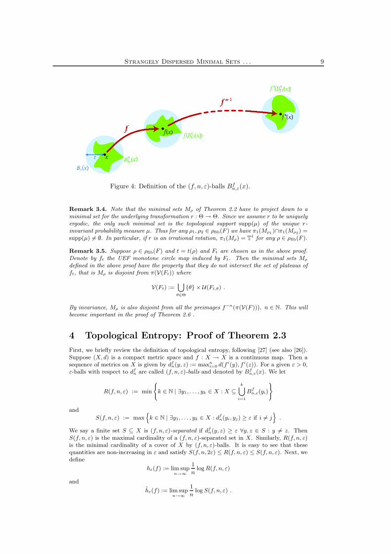
Figure 4: Definition of the (f, n, ε)-balls Bfn,ε(x).

Remark 3.4. Note that the minimal sets Mρ of Theorem 2.2 have to project down to aminimal set for the underlying transformation r : Θ → Θ. Since we assume r to be uniquelyergodic, the only such minimal set is the topological support supp(µ) of the unique r-invariant probability measure µ. Thus for any ρ1, ρ2 ∈ ρfib(F ) we have π1(Mρ1

)∩π1(Mρ2) =

supp(µ) 6= ∅. In particular, if r is an irrational rotation, π1(Mρ) = T1 for any ρ ∈ ρfib(F ).

Remark 3.5. Suppose ρ ∈ ρfib(F ) and t = t(ρ) and Ft are chosen as in the above proof.Denote by ft the UEF monotone circle map induced by Ft. Then the minimal sets Mρ

defined in the above proof have the property that they do not intersect the set of plateaus offt, that is Mρ is disjoint from π(V(Ft)) where

V(Ft) :=[

θ∈Θ

{θ} × U(Ft,θ) .

By invariance, Mρ is also disjoint from all the preimages f−n(π(V(F ))), n ∈ N. This willbecome important in the proof of Theorem 2.6 .

4 Topological Entropy: Proof of Theorem 2.3

First, we briefly review the definition of topological entropy, following [27] (see also [26]).Suppose (X, d) is a compact metric space and f : X → X is a continuous map. Then asequence of metrics on X is given by df

n(y, z) := maxni=0 d(f i(y), f i(z)). For a given ε > 0,

ε-balls with respect to dfn are called (f, n, ε)-balls and denoted by Bf

n,ε(x). We let

R(f, n, ε) := min

(

k ∈ N | ∃y1, . . . , yk ∈ X : X ⊆k

[

i=1

Bfn,ε(yi)

)

and

S(f, n, ε) := maxn

k ∈ N | ∃y1, . . . , yk ∈ X : dfn(yi, yj) ≥ ε if i 6= j

o

.

We say a finite set S ⊆ X is (f, n, ε)-separated if dfn(y, z) ≥ ε ∀y, z ∈ S : y 6= z. Then

S(f, n, ε) is the maximal cardinality of a (f, n, ε)-separated set in X. Similarly, R(f, n, ε)is the minimal cardinality of a cover of X by (f, n, ε)-balls. It is easy to see that thesequantities are non-increasing in ε and satisfy S(f, n, 2ε) ≤ R(f, n, ε) ≤ S(f, n, ε). Next, wedefine

hε(f) := lim supn→∞

1

nlog R(f, n, ε)

and

hε(f) := lim supn→∞

1

nlog S(f, n, ε) .


Again, these two quantities are non-increasing in ε, and the inequalities h2ε(f) ≤ hε(f) ≤hε(f) hold. The topological entropy of f is defined as

htop(f) := limε→0

hε(f) = supε>0

hε(f) ,

and from the preceding discussion it follows that we also have

htop(f) = limε→0

hε(f) = supε>0

hε(f) .

We remark that replacing the metric d by another metric d′ which is equivalent (mean-ing that d and d′ induce the same topology) does not change the topological entropy.In particular, there is no need to specify below which metric we choose on the productspace Θ × T1, any metric compatible with the product topology will do. However, forsimplicity we will assume the metric on Θ × T1 is chosen such that d((θ1, x1), (θ2, x2)) ≥max{d(θ1, θ2), d(x1, x2)}.

For the proof of Theorem 2.3, it will be convenient to work with a lift of the originalmap to a finite covering space of Θ× T1. Hence, we would like to know that this does notalter the topological entropy. We denote the k-fold cover of the circle by T1

k = R/kZ andwrite πk for the covering map πk : Θ × T1

k → Θ × T1.

Lemma 4.1. Suppose f : Θ × T1 → Θ × T1 is continuous and homotopic to the identity,let X = Θ × T1

k and assume f : X → X is a lift of f . Then htop(f) = htop(f).

Proof. A covering of X with (f , n, ε)-balls projects to a covering of Θ × T1 with (f, n, ε)-balls. Hence R(f, n, ε) ≤ R(f , n, ε) and thus htop(f) ≤ htop(f).

In order to prove the converse inequality, let ε0 ∈ (0, 14) be such that d(y, z) < ε0

implies d(f(y), f(z)) < 12

for all y, z ∈ X. We will show that for any 0 < ε ≤ ε0 we have

R(f , n, ε) ≤ kR(f, n, ε), which immediately implies htop(f) ≤ htop(f). Fix 0 < ε ≤ ε0, letR := R(f, n, ε) and choose y1, . . . , yR ∈ Θ×T1 such that Θ×T1 ⊆

SRi=1 Bf

n,ε(yi). For anyi ∈ {1, . . . , R}, the point yi has exactly k lifts zj

i (Figure 5), with d(zji , z

li) ≥ 1 whenever

j 6= l. We claim that X ⊆SR

i=1

Skj=1 Bf

n,ε(zji ), so R(f , n, ε) ≤ kR as required. In order to

see this, note that for any z ∈ X we must have πk(z) ∈ Bfn,ε(yi) for some i ∈ {1, . . . , R}.

In particular πk(z) ∈ Bε(yi), and therefore z ∈ Bε(zji ) for some j ∈ {1, . . . , k} (Figure 5).

Now πk(z) ∈ Bfn,ε(yi) implies that f(z) is contained in one of the k ε-balls that make up

(πk)−1Bε(f(yi)). All of these are pairwise disjoint and have distance ≥ 12

to each other,

since ε ≤ ε0 < 14. Due to the choice of ε0, we must have f(z) ∈ Bε(f(zj

i )). By induction

on m, we thus obtain fm(z) ∈ Bε(fm(zj

i )) for all m = 0, . . . , n. Hence z ∈ Bfn,ε(z

ji ). As

z ∈ X was arbitrary, this completes the proof.

Proof of Theorem 2.3 . Suppose f is a UEF circle endomorphism, homotopic to the iden-tity. Further, assume F is a lift of f and the rotation interval ρfib(F ) has non-emptyinterior. We will work with a lift f : X → X to the finite covering space X = Θ × T1

4 andshow that the numbers S(f , n, 1) grow exponentially.

For any ρ ∈ ρfib(F ), let Mρ be the minimal set provided by Theorem 2.2. Chooseρ1, ρ2 ∈ ρfib(F ) with ρ2 > ρ1 and let ǫ = 1

4(ρ2 − ρ1). Recall that π1(Mρ1

) ∩ π1(Mρ2) 6= ∅

(Remark 3.4). By the uniform convergence of the quantities 1n(F n

θ (x) − x) on Mρ1and

Mρ2there exists N ∈ N such that for any θ ∈ π1(Mρ1

) ∩ π1(Mρ2) we have for all n ≥ N

|F nθ (x1) − x1 − nρ1| < nǫ

|F nθ (x2) − x2 − nρ2| < nǫ

for any x1, x2 such that (θ, x1) ∈ π−1(Mρ1) and (θ, x2) ∈ π−1(Mρ2

). Thus

F nθ (x1) − x1 > nρ1 − nǫ

F nθ (x2) − x2 < nρ2 + nǫ


Figure 5: Illustration of the proof of Lemma 4.1, with z ∈ z21


Figure 6: Illustration of the proof of Theorem 2.3

so thatF n

θ (x1) − x1 + nρ2 + nǫ > F nθ (x2) − x2 + nρ1 − nǫ

and hence (recall that ρ2 − ρ1 = 4ǫ):

F nθ (x1) − F n

θ (x2) > x1 − x2 + n(ρ1 − ρ2 − 2ǫ)

> x1 − x2 + 2nǫ

By 3.1 we can take x2 − 1 < x1 < x2 without loss of generality. We then choose Nsufficiently large such that 2Nǫ > 5 and hence

F Nθ (x1) − F N

θ (x2) > 4

for any x1, x2 such that (θ, x1) ∈ π−1(Mρ1) and (θ, x2) ∈ π−1(Mρ2

) and x2 − 1 < x1 < x2.This implies that for any θ ∈ π1(Mρ1

) ∩ π1(Mρ2) the map fN

θ sends each of the intervalsIi := [i − 1, i] ⊆ T1

4, i = 1, . . . , 4 surjectively onto T14 (Figure 6). For any such θ and any

finite sequence σ ∈ {1, 3}n+1, n ∈ N of the symbols 1 and 3 define the set (Figure 7)

(4.1) Inσ := ∩n

i=0(fiNθ )−1(Iσi)


Figure 7: Construction of the Set Inσ defined by (4.1). The map fN

θ maps any of theintervals I1, . . . , I4 at least once around the whole of T1

4.

By definition, I0σ = Iσ0

and by the above Iσ1⊂ fN

θ (Iσ0). Hence fN

θ (I1σ) = Iσ1

. SimilarlyIσ2

⊂ fNθ (Iσ1

) = fNθ (fN

θ (I1σ)) = f2N

θ (I1σ) and so f2N

θ (I2σ) = Iσ2

. Continuing by inductionwe see that

f iNθ (In

σ ) = Iσi .

and in particular, Inσ is non-empty for any n ∈ N. Clearly, for any x ∈ In

σ and x′ ∈ Inσ′ with

σ 6= σ′, the points (θ, x) and (θ, x′) are (fN , n, 1)-separated. Thus S(fN , n, 1) ≥ 2n+1. ButS(f , nN, 1) ≥ S(fN , n, 1) and therefore

h1(f) = lim supn→∞

1

nlog S(f , n, 1)

≥ lim supn→∞

1

nNlog 2n+1 =

log 2

N> 0 .

Since by definition htop(f) ≥= h1(f) and htop(f) = htop(f) by Lemma 4.1, this completesthe proof.

The above proof shows that the positive entropy of f is even realised on single fibres,meaning that for suitable θ ∈ Θ we can find an exponentially growing number of (f, n, ε)-separated points contained in {θ} × T1. However, this is by no means surprising. In fact,when htop(r) = 0, as in the quasiperiodically forced case, it is the only way to obtainpositive topological entropy for the skew-product transformation. This follows from a well-known result by Bowen. In order to state it, we have to introduce the topological entropy ofa subset K ⊆ X, where as at the beginning of this section we assume that X is a compactmetric space. We let

R(f,K, n, ε) := min

(

k ∈ N | ∃y1, . . . , yk ∈ X : K ⊆k

[

i=1

Bfn,ε(yi)

)


and then define hε(f, K) := limn→∞1n

log R(f, K, n, ε) and htop(f, K) := limε→0 hε(f, K).

The numbers S(f, K, n, ε) and hε(f, K) are defined similarly, as above.

Theorem 4.2 (Bowen [27]). Suppose X, Z are compact metric spaces, r : X → X, f :Z → Z and p : Z → X are continuous maps, with p surjective and p ◦ f = r ◦ p. Then

htop(f) ≤ htop(r) + supy∈X

htop(f, p−1{y}) .

Hence, if f is a UEF circle endomorphism and htop(r) = 0, then htop(f) > 0 impliesthat there exists some θ ∈ Θ with htop(f, {θ} × T1) > 0. Conversely, if all fibre maps aremonotone then the above theorem easily entails the following

Corollary 4.3. Suppose f is a UEF monotone circle map. Then htop(f) = htop(r). Inparticular, if f is a QPF monotone circle map, then htop(f) = 0. Note that f need notnecessarily be homotopic to the identity.

Proof. For any θ ∈ Θ, let Tθ := {θ} × T1. In view of Theorem 4.2, we only have to provethat

htop(f, Tθ) = 0 ∀θ ∈ Θ .

In order to do so, we will show that the numbers R(f, Tθ, n, ε) can grow at most linearlywith n. To that end, fix θ0 ∈ Θ and ε > n. By compactness, there exists a finite cover ofΘ × T1 by boxes Ai

j = Ai × Ij , (i, j = 1, . . . , N), with the following properties:

(i) each set Aij has diameter less then ε;

(ii) there exist a0 < a1 <, . . . , < aN = a0 ∈ T1, such that Ij = [aj−1, aj ];

(iii) for all m ∈ N and j = 1, . . . , N , the point aj has a unique preimage under the mapfm

θ0;

Concerning (iii) note that, due to monotonicity, for each fibre map fθ the set of pointson which fθ is not injective is an at most countable union of intervals, and each of theseintervals is mapped to a single point. Consequently, for any m there is an at most countableset Em of exceptional points, whose preimage under fm

θ0is not unique. It suffices to choose

the aj outside the resulting countable unionS

m∈NEm.

We denote by An the n-th refinement of the cover A = {Aij | i, j ∈ {1, . . . , N}}, that is

An :=

(

α ⊆ Θ × T1

˛

˛

˛

˛

˛

α =n

\

k=0

f−k“

Aikjk

”

, ik, jk ∈ {1, . . . , N} ∀k = 0, . . . , n

)

.

By Anθ0

, we denote the restriction of An to the θ0-fibre, that is

Anθ0

:= {α ∩ Tθ0| α ∈ An} \ {∅} .

Choose points xβ ∈ Θ×T1, such that xβ ∈ β ∀β ∈ Anθ0

. Since the sets Aij all have diameter

less than ε, we obtain

Tθ0⊆

[

β∈Anθ0

Bfn,ε(xβ) .

Consequently, R(f, Tθ0, n, ε) ≤ #An

θ0where #An

θ0denotes the number of elements in the

partition Anθ0

. However, if k ∈ {0, . . . , n} is fixed, then due to montonicity and properties

(ii) and (iii) above the preimages of the intervals Ij under the map fkθ0

are all intervalswith pairwise disjoint interiors. It follows that An

θ is a partition of the circle Tθ0, given by

the points (θ0, (fkθ0

)−1(aj)), j = 1, . . . , N, k = 0, . . . , n. This implies that #Anθ ≤ (n+1)N ,

and consequently R(f,Tθ0, n, ε) ≤ (n + 1)N . Since θ0 ∈ Θ was arbitrary, this completes

the proof.

Proof of Theorem 2.2 (ii) . This follows immediately from Corollary 4.3. Recall fromthe proof of part (i) that the orbit under F of any point in Mρ coincides with the orbitunder the UEF monotone map Ft(ρ). Hence htop(f |Mρ) ≤ htop(ft(ρ)), where Ft(ρ) is a liftof ft(ρ). But, since Ft(ρ) is monotone we have htop(ft(ρ)) = 0, as required.


Figure 8: Essentially bounded sets on the torus. Green sets are essentially bounded, redsets are not.

5 Strangely Dispersed Minimal Sets: Proof of The-

orem 2.6

Let q : R2 → T2 = R2/Z2 denote the quotient map. We call a subset E ⊆ T2 essentiallybounded, if all connected components of q−1(E) are bounded, Figure 8. The followingproposition will be the key ingredient in the proof of Theorem 2.6 .

Proposition 5.1. Suppose f is a QPF circle endomorphism, homotopic to the identity.Further, assume E ⊆ T2 is open and essentially bounded and M ⊆ E is a minimal set.Then M is strangely dispersed.

Proof. Since M is minimal by assumption, it remains to show that it has properties (ii)and (iii) in Definition 2.4 .

In order to see that connected components of M are contained in single fibres, supposethat E0 is a connected component of E := q−1(E) such that M0 := q−1(M) ∩ E0 6= ∅.Since E is essentially bounded, E0 is bounded and hence M0 is compact. Thus the firstcoordinate of points in M0 attains a minimal value, at say (θ0, x0) ∈ M0 (more preciselyθ0 = inf{θ ∈ R | ∃x ∈ R : (θ, x) ∈ M0}). Let (θ0, x0) := q(θ0, x0) and E0 := q(E0).Observe that E0 ⊆ E is a connected component of E and in particular, E0 is open. Also(θ0, x0) ∈ M and (θ0, x0) ∈ E0

Now, assume that C ⊆ M is a connected component of M which is not containedin a single fibre. Then π1(C) is connected and hence an interval of positive length, sayπ1(C) = [a, b] with δ = d(a, b) > 0. We assume for simplicity of exposition that d(a, b) < 1

2.

Choose (θ, x) ∈ C with d(θ, a) = d(θ, b) = δ/2. Observe that for any n ∈ N, we haveπ1(f

n(C)) = [rn(a), rn(b)] which also has length δ, and d(θn, a) = d(θn, b) = δ/2 where(θn, xn) = fn(θ, x).

Since M is minimal, the orbit of (θ, x) is dense in M . By the above, E0 is openand contains (θ0, x0) ∈ M , so that there exists some n ∈ N, such that fn(θ, x) ∈ E0 ∩Bδ/4(θ0, x0). The set fn(C) is connected and fn(C) ⊆ M ⊆ E for all n ∈ N. Hencefn(C) is contained in a connected component of E. Since fn(C) contains fn(θ, x) ∈ E0

this connected component must by E0, that is fn(C) ⊆ E0.Define D0 as the unique connected component of q−1(fn(C)) that contains the unique

point (θ∗, x∗) in q−1{fn(θ, x)} ∩ Bδ/4(θ0, x0). Then (θ∗, x∗) ∈ E0, and by connectedness

D0 ⊆ E0 and hence D0 ⊆ M0. Since q(D0) = fn(C), q(θ∗, x∗) = fn(θ, x) = (θn, xn) andπ1(f

n(C)) = [θn − δ/2, θn + δ/2] we have π1(D0) = [θ∗ − δ/2, θ∗ + δ/2].But recall that θ0 = inf{θ ∈ R | ∃x ∈ R : (θ, x) ∈ M0}) and since D0 ⊆ M0 we must

have θ0 ≤ θ∗−δ/2. On the other hand (θ∗, x∗) ∈ Bδ/4(θ0, x0), so that θ∗ ≤ θ0+δ/4 which

implies that θ∗ − δ/2 ≤ θ0 − δ/4. Combining these two inequalities yields the contradiction

θ0 ≤ θ∗ − δ/2 ≤ θ0 − δ/4 .

Hence any connected component of M must be contained in a single fibre, proving property(ii).

It remains to prove that for any (θ, x) ∈ M and any open neighbourhood U of (θ, x),the set π1(U ∩ M) contains a non-empty open interval, i.e. property (iii). First observe


that if this property holds for some (θ, x) ∈ M then it holds for f(θ, x) (and hence fn(θ, x)for any n ∈ N). To see this, let U be an open neighbourhood of (θ, x). Then f−1(U) isan open neighbourhood of (θ, x), and hence π1(f

−1(U) ∩ M) contains a non-empty openinterval (a, b). Hence π1(U ∩ M) contains (r(a), r(b)) which has the same length as (a, b)and hence is a non-empty open interval. Also, property (iii) is closed, that is if it holdsfor a convergent sequence of points (θi, xi) ∈ M with (θi, xi) → (θ, x) then it holds for thelimit point (θ, x). This is because if U is an open neighbourhood U of (θ, x) then it is anopen neighbourhood of (θi, xi) for all sufficiently large i.

Thus, property (iii) is both closed and invariant and hence, it either holds for all orfor no point in M since by minimality the only closed invariant subsets of M are theempty set and M itself. Arguing by contradiction, let us assume that every z ∈ M hasa neighbourhood U(z), such that π1(U(z) ∩ M) contains no open interval and hence isnowhere dense. By compactness, M is covered by a finite number U(z1), . . . , U(zN ) of suchneighbourhoods. However, this would imply that π1(M) is the union of a finite numberof nowhere dense sets and hence is itself nowhere dense. This is clearly a contradiction,since π1(M) must be the whole circle, because this is the only closed invariant set of theunderlying irrational rotation.

Proof of Theorem 2.6. Suppose f is given by (1.1), and consequently has a lift F with fibremaps

Fθ(x) = x + τ +α

2πsin(2πx) + β sin(2πθ) .

Part (a). Recall that the QPF plateau maps Ft in the proof of Theorem 2.2 were givenby Ft,θ := (Fθ)t, with the mapping [0, 1] × E , (t, G) 7→ Gt provided by Proposition 3.1 .Any Ft induces a QPF monotone circle map, which we will denote by ft. If we let

G(x) := x + τ +α

2πsin(2πx) ,

then Ft,θ(x) = Gt(x) + β sin(2πθ). In particular, the plateaus of Ft,θ do not depend on θ.The fact that f in (1.1) is bimodal further implies that these plateaus are unique moduloaddition of integers, that is U(Gt) =

S

n∈ZIt +n for some interval It ⊆ R. Hence, recalling

Remark 3.5, we have (Figure 9a))

V(Ft) =[

θ∈T1

{θ} × U(Ft,θ) =[

k∈Z

T1 × (It + k) .

Now suppose that ρ ∈ ρfib(F ) and denote by Mρ the minimal set obtained in the proofof Theorem 2.2. Let t = t(ρ) ∈ [0, 1] be the corresponding parameter such that ρ(Ft) = ρand Mρ is a Ft-minimal set. As mentioned in Remark 3.5, Mρ is disjoint from the setS

n∈Nf−n(π(V(Ft)). Now if I ′ = [a, b] ⊆ It is a closed interval let

E := T2 \

`

T1 × π(I ′) ∪ f−1

t (T1 × π(I ′))´

,

as indicated in Figure 9(b,c). Then Mρ ⊆ E, and in view of Proposition 5.1 we only haveto show that E is essentially bounded. Since the complement q−1(E)c of q−1(E) containsthe horizontal line R × {a} and all its integer translates, it is obvious that all connectedcomponents of q−1(E) are bounded in the vertical direction.

We also claim that q−1(E)c contains a continuous curve joining R×{a} and R×{a+1},which implies immediately that it is bounded horizontally. We in fact show that V :=π−1(E) contains a continuous curve joining T1×{a+k} and T1×{a+k+1} for some k ∈ Z.Observe that F−1

t (T1 × I ′) contains a curve Γ that is the graph Γ := {(θ, γ(θ) | θ ∈ T1} ofa continuous function γ : T1 → R (Figure 9d). Since Γ is mapped into T1 × I ′ we have

Ft,θ(γ(θ)) = Gt(γ(θ)) + β sin(2πθ) ∈ I ′ ∀θ ∈ T1 .

Since we assume that β ≥ 32

we have

Ft,θ(γ(1/4)) = Gt(γ(1/4))) + β ≥ Gt(γ(1/4)) +3

2

Ft,θ(γ(3/4)) = Gt(γ(3/4)) − β ≤ Gt(γ(3/4)) −3

2.


(a) The set V(Ft) (b) The sets T1 × I′ and F−1t (T1 × I′).

(c) The set E, coloured yel-low, which is the lift of E =

T2 \“

T1 × π(I′) ∪ f−1t (T1 × π(I′))

”

(d) The curve Γ in F−1t (T1 × I′) and its

image under Ft in T1 × I′.

Figure 9: Proof of Theorem 2.6. Construction of the set E. This is given by the projectionto T2of the complement, coloured yellow, of T1 × I ′ (blue) and F−1

t (T1 × I ′) (green) inb).


Since the length of I ′ is less than 1 this implies

1 > Gt(γ(1/4)) +3

2− Gt(γ(3/4)) +

3

2

and henceGt(γ(3/4)) − Gt(γ(1/4)) > 2.

Since Gt is monotone and Gt(x + n) = Gt(x) + n ∀n ∈ Z, if γ(3/4) ≤ γ(1/4) + 2 thenGt(γ(3/4)) ≤ Gt(γ(1/4)+2) = Gt(γ(1/4))+2, so that Gt(γ(3/4))−Gt(γ(1/4)) ≤ 2. Hencewe must have γ(3/4) > γ(1/4) + 2, or in other words

γ(1/4) − γ(3/4) ≥ 2.

Hence there exists k ∈ Z, such that Γ intersects both T1 × {a + k} and T1 × {a + k + 1}.This proves our claim.

Part (b) Recall from the proof of Theorem 2.2 that ρfib(F ) = [ρ1, ρ2], where ρ1 = ρ(F−)and ρ(F2) = ρ(F+). For any x ∈ R, let x− := inf{y ∈ Z + 3

4| y ≥ x} and x+ := sup{y ∈

Z + 14| y ≤ x} (Figure 10). Then x− = x+ + 1

2or x− = x+ + 3

2. Note that

Fθ(x+) = x+ + τ +

α

2π+ β sin(2πθ)

Fθ(x−) = x− + τ −

α

2π+ β sin(2πθ)

and henceFθ(x

+) − Fθ(x−) = x+ − x− +

α

π.

Recall from the defintion of plateau maps that if x′ ≤ x then F−θ (x′) ≤ F (x) and

F+θ (x) ≥ F (x′). Since x+ ≤ x ≤ x− we have

F+θ (x) ≥ Fθ(x

+)

Fθ(x−) ≥ F−

θ (x)

for all (θ, x) ∈ T1 × R. Thus if α ≥ 52π, it follows that

F+θ (x) ≥ Fθ(x

+) ≥ Fθ(x−) +

5

2− (x− − x+) ≥ F−

θ (x) + 1 .

Hence we have F+θ (x) ≥ F−

θ (x)+1 for all (θ, x) ∈ T1×R, which implies ρ2 ≥ ρ1 +1. Henceρfib(F ) = [ρ1, ρ2] has positive length, as required.

References

[1] Grebogi, C., E. Ott, S. Pelikan and J.A. Yorke Strange attractors which are nor chaotic,Physica D 13:261–268, 1984.

[2] Ding, M., C. Grebogi and E. Ott Evolution of attractors in quasiperiodically forcedsystems - from quasiperiodic to strange nonchaotic to chaotic. Phys. Rev. A 39:2593–2598, 1989.

[3] Romeiras, F.J., A. Bondeson, E. Ott, T.M. Antonsen Jr. and C. Grebogi Quasiperiodi-cally forced dynamical systems with strange nonchaotic attractors. Physica D 26:277–294, 1987

[4] Romeiras, F.J., A. Bondeson, E. Ott, T.M. Antonsen Jr. and C. Grebogi Quasiperiodicforcing and the observability of strange nonchaotic attractors Phys. Scripta 40:442–444,1989.

[5] Romeiras, F.J. and E. Ott Strange nonchaotic attractors of the damped pendulum withquasiperiodic forcing. Phys. Rev. A 35:4404–4413, 1987.

[6] Feudel, U., J. Kurths and A.S. Pikovsky Strange nonchaotic attractor in a quasiperi-odically forced circle map Physica D 88:176–186, 1995.


Figure 10: Proof of the fact that F+

θ (x) ≥ F−

θ (x) + α/π − (x− − x+) We consider twocases: one where 1/4 ≤ x ≤ 3/4 (shown as x0) and the other where 3/4 ≤ x ≤ 7/4 (shownas x1). For both of these x+ = 1/4, whereas x− = 3/4 and 7/4 respectively, indicated asx−

0 and x−

1 on the figure.


[7] Pikovsky, A.S. and U. Feudel Characterizing strange nonchaotic attractors. Chaos5:253-260, 1995.

[8] Chastell, P. R., Glendinning, P. A., and Stark, J. Determining the locations of bifur-cations in quasiperiodic systems. Phys. Lett. A 200: 17–26. 1995.

[9] Glendinning, P., Feudel, U,, Pikovsky, A. S., and Stark, J. The structure of mode-lockedregions in quasi-periodically forced circle maps. Physica D 140: 227–243, 2000.

[10] Michael R. Herman. Une methode pour minorer les exposants de Lyapunov et quelquesexemples montrant le caractere local d’un theoreme d’Arnold et de Moser sur le torede dimension 2. Commentarii Mathematici Helvetici, 58:453–502, 1983.

[11] Keller, G. A note on strange nonchaotic attractors. Fundamenta Mathematicae 151:139–148, 1996.

[12] T. Jager. On the structure of strange non-chaotic attractors in pinched skew productsErgodic Theory and Dynamical Systems, 27:493–510, 2007.

[13] Glendinning, P. A., T. Jager and Keller, G. How chaotic are strange non-chaoticattractors? Nonlinearity 19:2005–2022, 2006.

[14] Stark, J., Invariant graphs for forced systems. Physica D 109: 163–179, 1997.

[15] Sturman, R., and Stark, J. Semi-uniform ergodic theorems and applications to forcedsystems. Nonlinearity 13:113–143, 2000.

[16] Kristian Bjerklov. Positive Lyapunov exponent and minimality for a class of one-dimensional quasi-periodic Schrodinger equations. Ergodic Theory and Dynamical Sys-tems, 25:1015–1045, 2005.

[17] T. Jager. The creation of strange non-chaotic attractors in non-smooth saddle-nodebifurcations. Preprint 2006, to appear in Memoirs of the AMS.

[18] T. Jager. Strange non-chaotic attractors in quasiperiodically forced circle maps.Preprint 2007.

[19] Stark, J., Feudel, U., Glendinning, P. A., and Pikovsky, A. Rotation numbers forquasi-periodically forced monotone circle maps. Dynamical Systems 17: 1–28, 2002.

[20] Stark, J. Transitive sets for quasi-periodically forced monotone maps DynamicalSystems 18: 351–364, 2003.

[21] T. Jager and G. Keller. The Denjoy type-of argument for quasiperiodically forcedcircle diffeomorphisms. Ergodic Theory and Dynamical Systems, 26(2):447–465, 2006.

[22] T. Jager and J. Stark Towards a classification for quasiperiodically forced circle home-omorphisms. J. London Math. Soc., 73:727–744, 2006.

[23] F. Beguin, S. Crovisier, T. Jager, and F. LeRoux. Denjoy constructions for fiberedhomeomorphisms of the two-torus. Preprint 2007.

[24] W. Huang and Y. Yi. Almost periodically forced circle flows. Preprint 2007.

[25] MacKay, R.S. and Tresser, C Transition to Topological Chaos for Circle Maps. PhysicaD 19:206–237, 1986.

[26] A. Katok and B. Hasselblatt. Introduction to the Modern Theory of Dynamical Sys-tems. Cambridge University Press, 1997.

[27] Rufus Bowen. Entropy for group endomorphisms and homogeneous spaces. Transac-tions of the AMS, 153:401–413, 1971.

[28] M. Misiurewicz and K. Ziemian. Rotation sets for maps of tori. Journal of the LondonMathematical Society, 40:490–506, 1989.

[29] M. Misiurewicz (2006) Rotation Theory. Online Proceedings of the RIMS Workshop”Dynamical Systems and Applications: Recent Progress” http://www.math.kyoto-u.ac.jp/ kokubu/RIMS2006/RIMS Online Proceedings.html

[30] P.L. Boyland. Bifurcations of circle maps: Arnold tongues, bistability and rotationintervals. Communications in Mathematical Physics, 106:353–381, 1986.

Strangely Dispersed Minimal Sets in the Quasiperiodically ...

Documents

Transcript of Strangely Dispersed Minimal Sets in the Quasiperiodically ...