STP-UDGAT: Spatial-Temporal-Preference User DimensionalGraph Attention Network for Next POI Recommendation

Nicholas Lim

GrabTaxi Holdings, Singapore

nic.lim@grab.com

Bryan Hooi

Grab-NUS AI Lab, National

University of Singapore, Singapore

dcsbhk@nus.edu.sg

See-Kiong Ng

Grab-NUS AI Lab, National

University of Singapore, Singapore

seekiong@nus.edu.sg

Xueou Wang

Grab-NUS AI Lab, National

University of Singapore, Singapore

idswx@nus.edu.sg

Yong Liang Goh

GrabTaxi Holdings, Singapore

yongliang.goh@grab.com

Renrong Weng

GrabTaxi Holdings, Singapore

renrong.weng@grab.com

Jagannadan Varadarajan

GrabTaxi Holdings, Singapore

jagan.varadarajan@grab.com

ABSTRACTNext Point-of-Interest (POI) recommendation is a longstanding

problem across the domains of Location-Based Social Networks

(LBSN) and transportation. Recent Recurrent Neural Network (RNN)

based approaches learn POI-POI relationships in a local view based

on independent user visit sequences. This limits the model’s abil-

ity to directly connect and learn across users in a global view to

recommend semantically trained POIs. In this work, we propose

a Spatial-Temporal-Preference User Dimensional Graph Attention

Network (STP-UDGAT), a novel explore-exploit model that con-

currently exploits personalized user preferences and explores new

POIs in global spatial-temporal-preference (STP) neighbourhoods,

while allowing users to selectively learn from other users. In addi-

tion, we propose random walks as a masked self-attention option

to leverage the STP graphs’ structures and find new higher-order

POI neighbours during exploration. Experimental results on six

real-world datasets show that our model significantly outperforms

baseline and state-of-the-art methods.

CCS CONCEPTS• Information systems→ Recommender systems.

KEYWORDSRecommender System; Graph Attention Network; Spatio-Temporal

ACM Reference Format:Nicholas Lim, Bryan Hooi, See-Kiong Ng, Xueou Wang, Yong Liang Goh,

Renrong Weng, and Jagannadan Varadarajan. 2020. STP-UDGAT: Spatial-

Temporal-Preference User Dimensional Graph Attention Network for Next

Permission to make digital or hard copies of all or part of this work for personal or

classroom use is granted without fee provided that copies are not made or distributed

for profit or commercial advantage and that copies bear this notice and the full citation

on the first page. Copyrights for components of this work owned by others than ACM

must be honored. Abstracting with credit is permitted. To copy otherwise, or republish,

to post on servers or to redistribute to lists, requires prior specific permission and/or a

fee. Request permissions from permissions@acm.org.

Conference’17, July 2017, Washington, DC, USA© 2020 Association for Computing Machinery.

ACM ISBN 978-x-xxxx-xxxx-x/YY/MM. . . $15.00

https://doi.org/10.1145/nnnnnnn.nnnnnnn

POI Recommendation. In Proceedings of ACM Conference (Conference’17).ACM,NewYork, NY, USA, 10 pages. https://doi.org/10.1145/nnnnnnn.nnnnnnn

1 INTRODUCTIONWith the increasing interest to provide personalized services, ser-

vice providers such as Location-Based Social Networks (LBSN) are

keen to understand their users better in order to do well on recom-

mendation tasks. Next Point-of-Interest (POI) recommendation has

been a longstanding problem for LBSNs to recommend places of

interest to their users. Recently, next POI recommendation has also

been found to be important for other applications. For instance,

ride-hailing services are interested to use next POI recommendation

to predict the next pick-up or drop-off points of their customers [7].

In the terrorism domain, it can be used to predict the likelihood of

the next state or city POI prone to be attacked by a terrorist group

[15].

Next POI recommendation is a challenging task due to its non-

linear patterns in user preferences. Early works explored conven-

tional collaborative filtering and sequential approaches such as

Matrix Factorisation (MF) and Markov Chains (MC) respectively.

For example, [3] extended the Factorizing Personalized Markov

Chain (FPMC) approach [16] that integrates both MF and MC, to

include localised region constraints and recommend nearby POIs

for the next POI recommendation task.

Recently, several works have proposed Recurrent Neural Net-

work (RNN) based approaches to better model the sequential de-

pendencies of users’ historical POI visits to learn their preferences,

as well as incorporating spatial and temporal factors in different

ways. [15] proposed a Spatial Temporal Recurrent Neural Network

(ST-RNN) to leverage spatial and temporal intervals between neigh-

bouring POIs, setting a time window to take several POIs as input.

[12] proposed the Hierarchical Spatial-Temporal Long-Short Term

Memory (HST-LSTM) to incorporate spatial and temporal intervals

directly into LSTM’s existing multiplicative gates. [30] proposed the

Spatio-Temporal Gated Coupled Network (STGCN) to capture short

and long-term user preference with new time and distance specific

arX

iv:2

010.

0702

4v1

[cs

.IR

] 6

Oct

202

0

gates. [17] proposed the Long- and Short-Term Preference Model-

ing (LSTPM) to learn long and short term user preferences through

the use of a nonlocal network and a geo-dilated RNN respectively.

With a clear trend towards learning user preferences from these

RNN-based approaches, a notable limitation is in how they learn

POI-POI relationships with a local view, where a POI is similar to

another POI if they tend to co-occur within individual users’ visit

sequences. This limits the model’s ability to directly learn POI-POI

relationships across all users in a global view through inter-user

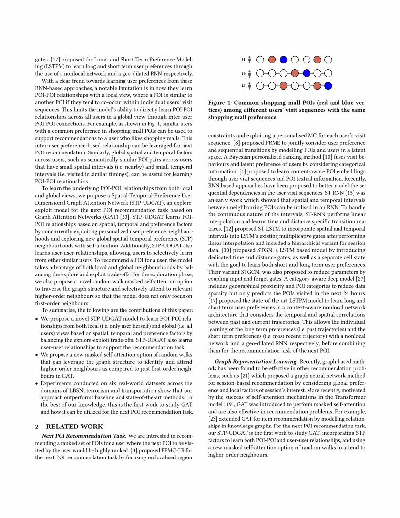
POI-POI connections. For example, as shown in Fig. 1, similar users

with a common preference in shopping mall POIs can be used to

support recommendations to a user who likes shopping malls. This

inter-user preference-based relationship can be leveraged for next

POI recommendation. Similarly, global spatial and temporal factors

across users, such as semantically similar POI pairs across users

that have small spatial intervals (i.e. nearby) and small temporal

intervals (i.e. visited in similar timings), can be useful for learning

POI-POI relationships.

To learn the underlying POI-POI relationships from both local

and global views, we propose a Spatial-Temporal-Preference User

Dimensional Graph Attention Network (STP-UDGAT), an explore-

exploit model for the next POI recommendation task based on

Graph Attention Networks (GAT) [20]. STP-UDGAT learns POI-

POI relationships based on spatial, temporal and preference factors

by concurrently exploiting personalized user preference neighbour-

hoods and exploring new global spatial-temporal-preference (STP)

neighbourhoods with self-attention. Additionally, STP-UDGAT also

learns user-user relationships, allowing users to selectively learn

from other similar users. To recommend a POI for a user, the model

takes advantage of both local and global neighbourhoods by bal-

ancing the explore and exploit trade-offs. For the exploration phase,

we also propose a novel random walk masked self-attention option

to traverse the graph structure and selectively attend to relevant

higher-order neighbours so that the model does not only focus on

first-order neighbours.

To summarise, the following are the contributions of this paper:

• We propose a novel STP-UDGAT model to learn POI-POI rela-

tionships from both local (i.e. only user herself) and global (i.e. all

users) views based on spatial, temporal and preference factors by

balancing the explore-exploit trade-offs. STP-UDGAT also learns

user-user relationships to support the recommendation task.

• We propose a new masked self-attention option of random walks

that can leverage the graph structure to identify and attend

higher-order neighbours as compared to just first-order neigh-

bours in GAT.

• Experiments conducted on six real-world datasets across the

domains of LBSN, terrorism and transportation show that our

approach outperforms baseline and state-of-the-art methods. To

the best of our knowledge, this is the first work to study GAT

and how it can be utilized for the next POI recommendation task.

2 RELATEDWORKNext POI Recommendation Task. We are interested in recom-

mending a ranked set of POIs for a user where the next POI to be vis-

ited by the user would be highly ranked. [3] proposed FPMC-LR for

the next POI recommendation task by focusing on localised region

Figure 1: Common shopping mall POIs (red and blue ver-tices) among different users’ visit sequences with the sameshopping mall preference.

constraints and exploiting a personalised MC for each user’s visit

sequence. [8] proposed PRME to jointly consider user preference

and sequential transitions by modelling POIs and users in a latent

space. A Bayesian personalized ranking method [10] fuses visit be-

haviours and latent preference of users by considering categorical

information. [1] proposed to learn content-aware POI embeddings

through user visit sequences and POI textual information. Recently,

RNN based approaches have been proposed to better model the se-

quential dependencies in the user visit sequences. ST-RNN [15] was

an early work which showed that spatial and temporal intervals

between neighbouring POIs can be utilised in an RNN. To handle

the continuous nature of the intervals, ST-RNN performs linear

interpolation and learns time and distance specific transition ma-

trices. [12] proposed ST-LSTM to incorporate spatial and temporal

intervals into LSTM’s existing multiplicative gates after performing

linear interpolation and included a hierarchical variant for session

data. [30] proposed STGN, a LSTM based model by introducing

dedicated time and distance gates, as well as a separate cell state

with the goal to learn both short and long term user preferences.

Their variant STGCN, was also proposed to reduce parameters by

coupling input and forget gates. A category-aware deep model [27]

includes geographical proximity and POI categories to reduce data

sparsity but only predicts the POIs visited in the next 24 hours.

[17] proposed the state-of-the-art LSTPM model to learn long and

short term user preferences in a context-aware nonlocal network

architecture that considers the temporal and spatial correlations

between past and current trajectories. This allows the individual

learning of the long term preferences (i.e. past trajectories) and the

short term preferences (i.e. most recent trajectory) with a nonlocal

network and a geo-dilated RNN respectively, before combining

them for the recommendation task of the next POI.

Graph Representation Learning. Recently, graph-based meth-

ods has been found to be effective in other recommendation prob-

lems, such as [24] which proposed a graph neural network method

for session-based recommendation by considering global prefer-

ence and local factors of session’s interest. More recently, motivated

by the success of self-attention mechanisms in the Transformer

model [19], GAT was introduced to perform masked self-attention

and are also effective in recommendation problems. For example,

[23] extended GAT for item recommendation by modelling relation-

ships in knowledge graphs. For the next POI recommendation task,

our STP-UDGAT is the first work to study GAT, incorporating STP

factors to learn both POI-POI and user-user relationships, and using

a new masked self-attention option of random walks to attend to

higher-order neighbours.

In the works of [21, 22, 29], they have shown the use of POI-POI

graphs to be helpful for learning POI semantics for other predictive

tasks. More related to our STP-UDGAT model is an early work

of GE [25] due to its usage of graphs. GE uses a POI-POI graph

and bipartite graphs of POI-Region, POI-Time and POI-Word to

learn node embeddings, then performs linear combinations of these

embeddings in its scoring function to output recommendations.

Our proposed STP-UDGAT has several key differences. First, STP-

UDGAT’s focus is on learning graph representations through GAT

and the masked self-attention process, whereas GE focuses on

learning node embeddings with LINE [18]; both methods have clear

differences in algorithm and optimization objectives. Second, our

POI-POI and User-User graphs are designed for use by GAT and

are not bipartite as bipartite graphs proposed in GE cannot be used

by GAT due to the different node types. Third, only STP-UDGAT

proposes to learn the balance of explore-exploit trade-offs among

the local (i.e. only user herself) and global (i.e. all users) views.

Additionally, STGCN [30] has showed GE to perform significantly

poorer as compared to basic recurrent baselines of RNN, GRU and

LSTM on all of their datasets for all metrics in their work, whereas

our STP-UDGAT does not just surpass these recurrent baselines,

but also the state-of-the-art LSTPM significantly.

3 PRELIMINARIESProblem Formulation. Let 𝑈 = {𝑢1, 𝑢2, ..., 𝑢𝑀 } be a set of 𝑀

users and 𝑉 = {𝑣1, 𝑣2, ..., 𝑣𝑁 } be a set of 𝑁 POIs for the users

in 𝑈 to visit. Each user 𝑢𝑚 has a sequence of POI visits 𝑠𝑢𝑚 =

{𝑣𝑡1 , 𝑣𝑡2 , ..., 𝑣𝑡𝑖 } and 𝑆 is the set of visit sequences for all users where𝑆 = {𝑠𝑢1

, 𝑠𝑢2, ..., 𝑠𝑢𝑀

}. The objective of the next POI recommenda-

tion task is to consider the historical POI visits {𝑣𝑡1 , 𝑣𝑡2 , ..., 𝑣𝑡𝑖−1 } anduser 𝑢𝑚 to recommend an ordered set of POIs from 𝑉 , where the

next POI visit 𝑣𝑡𝑖 should be highly ranked in the recommendation

set. We further denote 𝑉 𝑡𝑟𝑎𝑖𝑛, 𝑠𝑡𝑟𝑎𝑖𝑛𝑢𝑚

and 𝑆𝑡𝑟𝑎𝑖𝑛 as sets from the

training partition.

GAT. [20] follows the “masked” self-attention process (i.e. masked

to consider only adjacent vertices) to compute a hidden representa-

tion for vertex 𝑖 by attending to each vertex in its neighbourhood

set 𝑁 [𝑖] from a graph𝐺 . A single head GAT layer ΦΘ can be abbre-

viated as:

®𝑦𝑖 = ΦΘ (®𝑖, �̂�𝐴𝐺 [𝑖]) (1)

where ®𝑦𝑖 ∈ R𝛿 is the output hidden representation of the GAT layer

ΦΘ that accepts a tuple of (®𝑖, �̂�𝐴𝐺[𝑖]), ®𝑖 ∈ R𝑑 as the input represen-

tation of vertex 𝑖 and �̂�𝐴𝐺[𝑖] as the set of 𝑛 neighbours, where each

neighbour ®𝑗 ∈ �̂�𝐴𝐺[𝑖] has their own input representation ®𝑗 ∈ R𝑑 .

In �̂�𝐴𝐺[𝑖], the 𝑛 neighbours are determined from the closed neigh-

bourhood of vertex 𝑖 based on the adjacency option denoted as 𝐴

from a graph 𝐺 (i.e. first-order neighbours and vertex 𝑖 itself).

Given the input tuple (®𝑖, �̂�𝐴𝐺[𝑖]), a GAT layer first performs the

self-attention process by computing scalar attention coefficients

𝛼𝑖 𝑗 ∈ R for each neighbouring vertex’s representation ®𝑗 ∈ �̂�𝐴𝐺[𝑖] in

the scale of 0 and 1, where 1 means “completely attend vertex 𝑗” and

0 means “completely ignore vertex 𝑗”. This involves the use of an

input projection weight matrix W𝑝 ∈ R𝑑×𝛿 and a linear projection

a parameterized with {W𝑎 ∈ R2𝛿 , b𝑎 ∈ R}:

𝛼𝑖 𝑗 =

𝑒𝑥𝑝

(𝐿𝑒𝑎𝑘𝑦𝑅𝑒𝐿𝑈

(a [W𝑝®𝑖 | | W𝑝 ®𝑗]

))∑

®𝑘∈�̂�𝐴𝐺[𝑖 ] 𝑒𝑥𝑝

(𝐿𝑒𝑎𝑘𝑦𝑅𝑒𝐿𝑈

(a [W𝑝®𝑖 | | W𝑝

®𝑘])) (2)

where | | is the concatenation operation, 𝐿𝑒𝑎𝑘𝑦𝑅𝑒𝐿𝑈 as the non-

linear activation function and the softmax function to output the

attention coefficients as a probability distribution that sums to 1

for all 𝑛 neighbours. With the learned coefficients, a weighted sum

between vertex 𝑖 and its neighbours in �̂�𝐴𝐺[𝑖] is then computed as

the output hidden representation of the GAT layer ΦΘ:

®𝑦𝑖 =∑︁

®𝑗 ∈�̂�𝐴𝐺[𝑖 ]𝛼𝑖 𝑗W𝑝 ®𝑗 (3)

4 APPROACHOur approach is to learn POI-POI and user-user relationships from

both local (i.e. only user herself) and global (i.e. all users) views

based on STP factors. In this section, we first propose the Dimen-

sional GAT (DGAT) to learn attention coefficients across dimen-

sions to improve the self-attention process. Then, we introduce the

Personalized-Preference DGAT (PP-DGAT) to exploit each user’s

historical POI visits or local POI preferences, followed by extending

it to Spatial-Temporal-Preference DGAT (STP-DGAT) that not only

performs the same exploitation of users’ local POI preferences, but

also includes the exploration of global STP graphs to consider new

POIs which the user has never visited before, as well as balancing

the explore-exploit trade-offs among the local (exploit) and global

(explore) views. Lastly, we further introduce UDGAT (User-DGAT)

to allow users to learn to attend to other similar users.

4.1 DGATIn a GAT layer, the self-attention process first computes scalar

attention coefficients with a shared linear projection a for each

neighbour ®𝑗 ∈ �̂�𝐴𝐺[𝑖] in the scale of 0 and 1, as per Eq. (2). Then, in

Eq. (3), the predicted coefficients are used for a weighted sum to

compute a hidden representation ®𝑦𝑖 accordingly. This processmakes

a key assumption where the scalar coefficients are representative of

the whole vector representation for each neighbour ®𝑗 ∈ �̂�𝐴𝐺[𝑖]. We

argue that self-attention can be applied to each dimension of ®𝑗 tobetter leverage the latent semantics, where each dimension would

have its own coefficient. To extend the scalar attention coefficients

(GAT) to dimensional attention coefficients (DGAT), first, wemodify

the linear projection a to predict 𝛿 dimensional coefficients instead

of 1 (i.e. {W𝑎 ∈ R2𝛿 , b𝑎 ∈ R} to {W𝑎 ∈ R2𝛿×𝛿 , b𝑎 ∈ R𝛿 }), resultingEq. (2) to output ®𝛼𝑖 𝑗 ∈ R𝛿 instead of scalar 𝛼𝑖 𝑗 ∈ R. Secondly, wereplace Eq. (3) with:

®𝑦𝑖 =∑︁

®𝑗 ∈�̂�𝐴𝐺[𝑖 ]

®𝛼𝑖 𝑗 ⊙ W𝑝 ®𝑗 (4)

where ⊙ is the Hadamard product to achieve the intention of DGAT.

4.2 PP-DGATApplying DGAT to the next POI recommendation problem is not a

straight forward task. For instance, given the historical POI visits

{𝑣𝑡1 , 𝑣𝑡2 , ..., 𝑣𝑡𝑖−1 } for a user 𝑢𝑚 , we would like to predict the next

POI 𝑣𝑡𝑖 . We can use the previous POI 𝑣𝑡𝑖−1 as input to the DGAT layer

to output a hidden representation from the masked self-attention

process by attending to a set of reliable reference POI neighbours

𝑁𝐴𝐺[𝑣𝑡𝑖−1 ] queried from a graph𝐺 given 𝑣𝑡𝑖−1 , however, it is unclear

how this neighbourhood and graph can be constructed such that the

queried closed neighbourhood 𝑁𝐴𝐺[𝑣𝑡𝑖−1 ] (i.e. adjacent POI vertices

and 𝑣𝑡𝑖−1 itself) are indeed relevant to vertex 𝑣𝑡𝑖−1 and can benefit

the overall prediction task.

Definition 1 (personalized preference graph). An undi-rected complete POI-POI graph for each user 𝑢𝑚 ∈ 𝑈 , denoted as𝑢𝐺𝑚 = (𝑉𝑢𝑚 , 𝐸𝑢𝑚 ) where 𝑉𝑢𝑚 and 𝐸𝑢𝑚 are the sets of POIs and un-weighted edges respectively. We set 𝑉𝑢𝑚=𝑠𝑡𝑟𝑎𝑖𝑛𝑢𝑚

and all pairs of POIvertices are connected, forming a complete graph that represents theuser’s historical POI preferences.

Learning From Local View. As per Definition 1, we propose to

construct a fully connected or complete Personalized Preference

(PP) graph𝑢𝐺𝑚 from each user’s set of historical training POIs 𝑠𝑡𝑟𝑎𝑖𝑛𝑢𝑚,

where 𝑢𝐺𝑚 can be actively queried for 𝑁𝐴𝐺[𝑣𝑡𝑖−1 ] in each time step

of the prediction by a DGAT layer. Fig. 2 illustrates how a user’s

available historical POIs 𝑠𝑡𝑟𝑎𝑖𝑛𝑢𝑚are used to construct a PP graph

that serves to be queried by the DGAT layer for the closed neigh-

bourhood 𝑁𝐴𝐺[𝑣𝑡𝑖−1 ] when given input of 𝑣𝑡𝑖−1 and performing the

self-attention process. Accordingly, this would also mean that each

user 𝑢𝑚 will have her own PP graph 𝑢𝐺𝑚 that encapsulate her own

“local” historical preferences without clear consideration of other

users’ POI visiting behaviors to learn POI-POI relationships. This

enables personalization by exploiting only the user’s individual

preferences from a local view as personalization has been shown

by past works (e.g. FPMC-LR [3]) to surpass “global” methods that

consider all users’ behaviors directly (e.g. MC).

Next, we describe the PP-DGAT in detail. Given a previous visit

POI 𝑣𝑡𝑖−1 as input, we query the user’s PP graph𝑢𝐺𝑚 for𝑁𝐴

𝑢𝐺𝑚[𝑣𝑡𝑖−1 ] as

the set of reference POI neighbours and is equivalent to all vertices

𝑉𝑢𝑚 in 𝑢𝐺𝑚 due to the completeness design of the PP graph and

the closed neighbourhood nature of the query (i.e. including 𝑣𝑡𝑖−1 ).

This essentially allows the DGAT layer to perform self-attention

on all historical training POIs of the user because 𝑉𝑢𝑚=𝑠𝑡𝑟𝑎𝑖𝑛𝑢𝑚by

definition. Then, we provide both 𝑣𝑡𝑖−1 and 𝑁𝐴

𝑢𝐺𝑚[𝑣𝑡𝑖−1 ] to 𝐸𝑚𝑏 as

an input tuple, where 𝐸𝑚𝑏 is an embedding layer, parameterised

by the POI weight matrix W𝑝𝑜𝑖 ∈ R |𝑉 |×𝑑𝑖𝑚and 𝑑𝑖𝑚 is the defined

embedding dimension. Accordingly, 𝐸𝑚𝑏 outputs the tuple of the

corresponding POI embedding representations (®𝑣𝑡𝑖−1 , �̂�𝐴

𝑢𝐺𝑚[𝑣𝑡𝑖−1 ]),

®𝑣𝑡𝑖−1 as the embedding of the previous POI 𝑣𝑡𝑖−1 , and �̂�𝐴

𝑢𝐺𝑚[𝑣𝑡𝑖−1 ] as

the set of embeddings of all the neighbors of 𝑣𝑡𝑖−1 :

(®𝑣𝑡𝑖−1 , �̂�𝐴

𝑢𝐺𝑚[𝑣𝑡𝑖−1 ]) = 𝐸𝑚𝑏W𝑝𝑜𝑖 (𝑣𝑡𝑖−1 , 𝑁𝐴

𝑢𝐺𝑚[𝑣𝑡𝑖−1 ]) (5)

®𝑦𝑡𝑖 = ΦW𝑃𝑃 (®𝑣𝑡𝑖−1 , �̂�𝐴

𝑢𝐺𝑚[𝑣𝑡𝑖−1 ]) (6)

𝑃 (𝑣𝑡𝑖 |𝑣𝑡𝑖−1 ) = 𝑠𝑜 𝑓 𝑡𝑚𝑎𝑥 (𝐹𝐶W𝑓 1 ( 𝐷 ( ®𝑦𝑡𝑖 ) )) (7)

Using a DGAT layer ΦW𝑃𝑃 , Eq. (6) computes the hidden representa-

tion ®𝑦𝑡𝑖 and Eq. (7) linearly projects ®𝑦𝑡𝑖 to the number of classes or

POIs (i.e. |𝑉 |) followed by a softmax functionwhere𝐷 is the dropout

layer, 𝐹𝐶W𝑓 1∈R𝛿×|𝑉 | as a linear Fully Connected (FC) layer. With

the probability distribution of all POIs in 𝑉 by learning 𝑃 (𝑣𝑡𝑖 |𝑣𝑡𝑖−1 )

Figure 2: Illustration of self-attention performed on a user’sPP graph based on her historical POIs.

as a multi-classification problem, we would have the final ranked

POI recommendation set by sorting it in descending order. At test

time, we follow the same as training to perform self-attention on

all vertices of the user’s PP graph (i.e. all user’s available historical

POIs).

4.3 STP-DGATWith PP-DGAT, next POI predictions can be computed from just the

exploitation of the users’ historical POIs 𝑠𝑡𝑟𝑎𝑖𝑛𝑢𝑚or local preferences.

However, this limits the learning of POI-POI relationships for the

recommendation task by not considering global spatial, temporal

and preference factors. For example, a user who likes shopping mall

may be interested in visiting new nearby malls (spatial), or perhaps

new malls that are popular only at night (temporal), or new malls

which other similar users of the same shopping mall interest have

visited (preference). Here, a new POI 𝑣𝑛 refers to an unvisited POI

in the user’s historical POI visits (i.e. 𝑣𝑛 ∉ 𝑠𝑡𝑟𝑎𝑖𝑛𝑢𝑚). We propose to

not only consider local user POI preferences as done in PP-DGAT,

but also global STP factors across all users to improve the recom-

mendation task and user experience [31] through the exploration

of new unvisited POIs to better learn the POI-POI relationships.

Although personalization has been shown by existing works to

learn the users’ semantics well, we believe that new unvisited POIs

identified across global STP factors can also be leveraged in a way

that does not jeopardize personalization. We propose to achieve this

by learning the balance between the exploitation of the user’s local

preference or personalization and the exploration of new unvisited

POIs based on the global STP factors for the task.

Definition 2 (Spatial Graph). An undirected POI-POI graphdenoted as 𝐺𝑠 = (𝑉𝑠 , 𝐸𝑠 ) where 𝑉𝑠 and 𝐸𝑠 are the sets of POIs andedges respectively and we set 𝑉𝑠 = 𝑉 . POI 𝑣𝑖 has adjacency to POI 𝑣 𝑗if 𝑣 𝑗 is within the top 𝜎 nearest POIs based on the distance intervalΔ𝑑 using a distance function 𝑑 (𝑣𝑖 , 𝑣 𝑗 ). We set 𝜎 = 5 and 𝑑 (𝑣𝑖 , 𝑣 𝑗 ) asEuclidean distance. The edge weight between each pair is 1

Δ𝑑 .

Definition 3 (Temporal Graph). An undirected POI-POI graphdenoted as𝐺𝑡 = (𝑉𝑡 , 𝐸𝑡 ) where𝑉𝑡 and 𝐸𝑡 are the sets of POIs and edgesrespectively and 𝑉𝑡 = 𝑉 𝑡𝑟𝑎𝑖𝑛 . As each POI visit includes timestampdata, we first combine all users’ historical POI visit sequence 𝑠𝑢𝑚 ∈𝑆𝑡𝑟𝑎𝑖𝑛 to a single set of 𝑆𝑡𝑟𝑎𝑖𝑛

𝑡𝑖𝑚𝑒that disregards which user the POI

visits belong to and have all POI visits sorted in chronological order.Then, we compute POI pairs from 𝑆𝑡𝑟𝑎𝑖𝑛

𝑡𝑖𝑚𝑒where POI 𝑣𝑖 is adjacent to

𝑣 𝑗 if 𝑣 𝑗 is the next visit based on chronological order. The edge weightbetween each pair is 1

Δ𝑡where Δ𝑡 is the averaged time interval of all

same pairs.

Figure 3: Illustration of how global spatial, temporal and preference factors are represented into POI-POI graphs. Maps ©OpenStreetMap contributors, CC BY-SA.

Definition 4 (PreferenceGraph). An undirected POI-POI graphdenoted as 𝐺𝑝 = (𝑉𝑝 , 𝐸𝑝 ) where 𝑉𝑝 and 𝐸𝑝 are the sets of POIs andedges respectively and we set 𝑉𝑝 = 𝑉 𝑡𝑟𝑎𝑖𝑛 . POI pairs are computedfrom each user’s visit sequence 𝑠𝑢𝑚 ∈ 𝑆𝑡𝑟𝑎𝑖𝑛 where POI 𝑣𝑖 is adjacentto 𝑣 𝑗 if 𝑣 𝑗 is the next visit. The edge weight between each pair is𝑓 𝑟𝑒𝑞(𝑣𝑖 , 𝑣 𝑗 ) where 𝑓 𝑟𝑒𝑞 is the count function of POI pair occurrences.

Representing STP Factors. From Definitions 2 to 4, we propose

the spatial, temporal and preference POI-POI graphs to embed the

semantics of global STP factors, for the purpose of being utilized

by DGAT layers to explore new POIs and leveraging them for

the recommendation task. Fig. 3 illustrate examples of how the

STP factors are represented into POI-POI graphs and its intentions

(whole graph not shown). For instance, in Fig. 3, spatial graph 𝐺𝑠

connects each POI (orange node) in 𝑉 to its nearest top 5 POIs to

embed geographical proximities; temporal graph 𝐺𝑡 connects POIs

in 𝑆𝑡𝑟𝑎𝑖𝑛𝑡𝑖𝑚𝑒

, as per definition, connecting POIs that are similar in visit

timestamps across all users and disregarding which user the POI

visit it belongs to. This allows schools and bus stations POIs to be

connected during day time, and similarly so for bars and clubs POIs

at night even when they do not co-occur in a user’s historical POI

visit sequence. Preference graph 𝐺𝑝 connects POIs sequentially

across each user’s sequence for all users, allowing POI vertices to

connect in a global preference view by considering all users and

connecting similar sequences, which contrasts with a PP graph that

only considers the historical POIs of the user herself.

Exploring New STP Neighbours. With the proposed graphs,

we would like to find new POIs from STP graphs which the user

has never visited before, but yet are relevant to the user and can help

better learn POI-POI relationships. We propose to use all vertices

𝑉𝑢𝑚 in the user’s PP graph𝑢𝐺𝑚 as the set of seed POIs to find relevant

new POIs in STP graphs. As all vertices 𝑉𝑢𝑚 is equivalent to the

user’s historical POIs, 𝑉𝑢𝑚 = 𝑠𝑡𝑟𝑎𝑖𝑛𝑢𝑚as per Definition 1, this allows

us to find relevant neighbours based on the entire vertex set. First,

we compute the closed neighbourhood of each POI in the user’s PP

graph vertex set {𝑁𝐴𝐺[𝑣𝑖 ] | 𝑣𝑖 ∈ 𝑉𝑢𝑚 } through the adjacency option

𝐴 from a graph𝐺 , then, we remove all visited POIs by the user and

perform a frequency ranking to compute the top 𝜏 new neighbours,

denoting this result set 𝑁𝐴𝐺(𝑉𝑢𝑚 )𝜏 as the open neighbourhood of

𝑉𝑢𝑚 (i.e. excluding POIs in 𝑉𝑢𝑚 to keep only newly discovered

POIs). We thus identify 𝑁𝐴𝐺(𝑉𝑢𝑚 )𝜏 for all proposed STP graphs

Figure 4: Input previous POI of 𝑣𝑡𝑖−1 (blue vertex) andnext POI of 𝑣𝑡𝑖 (red vertex). Green vertices are first-orderneighbours and orange vertices are higher-order neighboursfound with random walks.

𝐺𝑆𝑇𝑃 = {𝐺𝑠 ,𝐺𝑡 ,𝐺𝑝 } and mapping them to POI representations

with Eq. (5). Then, we use separate DGAT layers and perform mean

pooling to output a single STP representation ®𝑜𝐴𝑡𝑖 :

®𝑜𝐴𝑡𝑖 =1

|𝐺𝑆𝑇𝑃 |∑︁

𝐺 ∈𝐺𝑆𝑇𝑃

W∈{W𝐴𝑆,W𝐴

𝑇W𝐴

𝑃}

ΦW (®𝑣𝑡𝑖−1 , �̂�𝐴𝐺 (𝑉𝑢𝑚 )𝜏 ) (8)

Random Walk Masked Self-Attention. To ensure that the ex-

ploration of new POIs in STP graphs is not limited to just new

first-order neighbours using adjacency option 𝐴, we propose an

alternative approach of random walks that have been shown to be

effective in exploring diverse neighbourhoods of graphs in other

applications [9], where 𝑁𝑅𝑊𝐺

(𝑉𝑢𝑚 )𝜏 is the top 𝜏 new STP neigh-

bours found with random walk masked self-attention option 𝑅𝑊

to focus on higher-order neighbours. Fig. 4 illustrates the problem

where first-order neighbours are insufficient to represent the neigh-

bourhood of vertex 𝑣𝑡𝑖−1 , a shopping mall, and can benefit from

higher-order vertices as determined by the random walks, such as

nearby metros to correctly predict 𝑣𝑡𝑖 , a metro. As per Definitions

2 to 4 and Fig. 3, we set the edge weights of STP graphs as1

Δ𝑑 ,1

Δ𝑡and 𝑓 𝑟𝑒𝑞(𝑣𝑖 , 𝑣 𝑗 ) respectively. This intentionally biases the random

walks to nearby POIs (spatial), POIs visited in similar timings (tem-

poral) and popular POIs visited by other similar users (preference).

The total random walk POIs for a graph 𝐺 (𝑉 , 𝐸) is computed as

|𝑉 | × ` × 𝛽 where ` is the number of random walks per vertex and

𝛽 is the walk’s length.

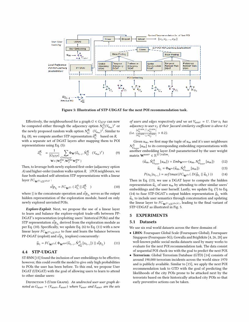
Figure 5: Illustration of STP-UDGAT for the next POI recommendation task.

Effectively, the neighbourhood for a graph 𝐺 ∈ 𝐺𝑆𝑇𝑃 can now

be computed either through the adjacency option 𝑁𝐴𝐺(𝑉𝑢𝑚 )𝜏 or

the newly proposed random walk option 𝑁𝑅𝑊𝐺

(𝑉𝑢𝑚 )𝜏 . Similar to

Eq. (8), we compute another STP representation ®𝑜𝑅𝑊𝑡𝑖 based on 𝑅𝑊

with a separate set of DGAT layers after mapping them to POI

representations using Eq. (5):

®𝑜𝑅𝑊𝑡𝑖 =1

|𝐺𝑆𝑇𝑃 |∑︁

𝐺 ∈𝐺𝑆𝑇𝑃

W∈{W𝑅𝑊𝑆

,W𝑅𝑊𝑇

W𝑅𝑊𝑃

}

ΦW (®𝑣𝑡𝑖−1 , �̂�𝑅𝑊𝐺

(𝑉𝑢𝑚 )𝜏 ) (9)

Then, to leverage both newly explored first-order (adjacency option

𝐴) and higher-order (randomwalks option 𝑅𝑊 ) POI neighbours, we

fuse both masked self-attention STP representations with a linear

layer 𝐹𝐶W𝑓 2∈R2𝛿×𝛿 :

®𝑠𝑡𝑝𝑡𝑖 = 𝐹𝐶W𝑓 2 ( ®𝑜𝐴𝑡𝑖 | | ®𝑜𝑅𝑊𝑡𝑖

) (10)

where | | is the concatenate operation and ®𝑠𝑡𝑝𝑡𝑖 serves as the outputhidden representation of the exploration module, based on only

newly explored unvisited POIs.

Explore-Exploit. Next, we propose the use of a linear layer

to learn and balance the explore-exploit trade-offs between PP-

DGAT’s representation (exploiting users’ historical POIs) and the

STP representation ®𝑠𝑡𝑝𝑡𝑖 derived from the exploration module as

per Eq. (10). Specifically, we update Eq. (6) to Eq. (11) with a new

linear layer 𝐹𝐶W𝑓 3∈R2𝛿×𝛿 to fuse and learn the balance between

PP-DGAT (exploit) and ®𝑠𝑡𝑝𝑡𝑖 (explore) concurrently:

®𝑦𝑡𝑖 = 𝐹𝐶W𝑓 3 ( ΦW𝑃𝑃 (®𝑣𝑡𝑖−1 , �̂�𝐴

𝑢𝐺𝑚[𝑣𝑡𝑖−1 ]) | | ®𝑠𝑡𝑝𝑡𝑖 ) (11)

4.4 STP-UDGATST-RNN [15] found the inclusion of user embeddings to be effective;

however, this could overfit the model to give only high probabilities

to POIs the user has been before. To this end, we propose User

DGAT (UDGAT) with the goal of allowing users to learn to attend

to other similar users:

Definition 5 (User Graph). An undirected user-user graph de-noted as 𝐺𝑢𝑠𝑒𝑟 = (𝑉𝑢𝑠𝑒𝑟 , 𝐸𝑢𝑠𝑒𝑟 ) where 𝑉𝑢𝑠𝑒𝑟 and 𝐸𝑢𝑠𝑒𝑟 are the sets

of users and edges respectively and we set 𝑉𝑢𝑠𝑒𝑟 = 𝑈 . User 𝑣𝑖 hasadjacency to user 𝑣 𝑗 if their Jaccard similarity coefficient is above 0.2

(i.e.|𝑠𝑡𝑟𝑎𝑖𝑛𝑣𝑖

⋂𝑠𝑡𝑟𝑎𝑖𝑛𝑣𝑗

||𝑠𝑡𝑟𝑎𝑖𝑛𝑣𝑖

⋃𝑠𝑡𝑟𝑎𝑖𝑛𝑣𝑗

| > 0.2).

Given 𝑢𝑚 , we first map the tuple of 𝑢𝑚 and it’s user neighbours

𝑁𝐴𝐺𝑢𝑠𝑒𝑟

[𝑢𝑚] to its corresponding embedding representations with

another embedding layer 𝐸𝑚𝑏 parameterised by the user weight

matrixW𝑢𝑠𝑒𝑟 ∈ R |𝑈 |×𝑑𝑖𝑚:

(®𝑢𝑚, �̂�𝐴𝐺𝑢𝑠𝑒𝑟

[𝑢𝑚]) = 𝐸𝑚𝑏W𝑢𝑠𝑒𝑟 (𝑢𝑚, 𝑁𝐴𝐺𝑢𝑠𝑒𝑟

[𝑢𝑚]) (12)

®𝑢𝑡𝑖 = ΦW𝑢 (®𝑢𝑚, �̂�𝐴𝐺𝑢𝑠𝑒𝑟

[𝑢𝑚]) (13)

𝑃 (𝑣𝑡𝑖 |𝑣𝑡𝑖−1 ) = 𝑠𝑜 𝑓 𝑡𝑚𝑎𝑥 (𝐹𝐶W𝑓 1 ( 𝐷 ( ®𝑦𝑡𝑖 | | ®𝑢𝑡𝑖 ) )) (14)

Then in Eq. (13), we use a DGAT layer to compute the hidden

representation ®𝑢𝑡𝑖 of user 𝑢𝑚 by attending to other similar users’

embeddings and the user herself. Lastly, we update Eq. (7) to Eq.

(14) to fuse STP-DGAT’s output hidden representation ®𝑦𝑡𝑖 with®𝑢𝑡𝑖 to include user semantics through concatenation and updating

the linear layer to 𝐹𝐶W𝑓 1∈R2𝛿×|𝑉 | , leading to the final variant of

STP-UDGAT as illustrated in Fig. 5.

5 EXPERIMENTS5.1 DatasetsWe use six real world datasets across the three domains of:

• LBSN: Foursquare Global Scale (Foursquare-Global), Foursquare

Singapore (Foursquare-SG), Gowalla and Brightkite [4, 26, 28] are

well-known public social media datasets used by many works to

evaluate for the next POI recommendation task. The data consist

of sequential POI check-ins with the goal to predict the next POI.

• Terrorism: Global Terrorism Database (GTD) [14] consists of

around 190,000 terrorism incidents across the world since 1970

and is publicly available. Similar to [15], we apply the next POI

recommendation task to GTD with the goal of predicting the

likelihoods of the city POIs prone to be attacked next by the

terrorists based on their historically attacked city POIs so that

early preventive actions can be taken.

• Transportation: Different from taxi trajectory datasets [2] that

record taxi-visited POIs from multiple different customers for

the same taxi, user trajectory datasets instead record the taxi

riding patterns from the same user, and are privately available to

ride-hailing companies such as Uber, Didi, and others through the

use of their mobile applications. Here, we use a user trajectory

dataset of a Southeast Asia (SEA) country (Transport-SEA) from

the ride-hailing company Grab to predict the next drop-off point

POI based on the user’s historical drop-off point POIs.

Table 1 shows the details of the datasets. For preprocessing,

we group the datasets into Large and Small Scale categories and

only keep POIs visited by more than 10 users for all datasets. We

keep users with visit counts between 10 and 30 for Large Scale

datasets, and between 10 and 150 for Small Scale datasets. For only

the Foursquare-Global dataset, we take the top 40 popular countries

by the number of visits. Lastly, we sort each user’s visit records by

timestamps in ascending order, taking the first 70% as training set

and remaining 30% as testing set.

5.2 Baseline Methods and Evaluation Metrics• TOP and U-TOP: These rank POIs using frequencies across

𝑆𝑡𝑟𝑎𝑖𝑛 and in 𝑠𝑡𝑟𝑎𝑖𝑛𝑢𝑚respectively.

• MF [13]: MF is a popular classical approach to many recommen-

dation problems.

• RNN [6]: RNN takes advantage of sequential dependencies in

POI visit sequences with a basic recurrent structure. LSTM [11]

and GRU [5] are variants of RNN with different multiplicative

gates.

• HST-LSTM [12]: This method incorporates spatial and temporal

intervals into LSTM gates. Same as [30], we use the ST-LSTM

variant here as the data does not include session information.

• STGN [30]: An LSTM variant that models both short and long

term POI visit preferences with new time and distance gates, and

cell state. The coupled gate variant STGCN removes the forget

gate for better efficiency.

• LSTPM [17]: An LSTM-based model that captures long term

preferences with a nonlocal network and short term preferences

with a geo-dilated network. LSTPM is the state-of-the-art method

for the next POI recommendation task.

For our proposed model, we evaluate with the following variants:

• PP-DGAT-Skip: Our proposed PP-DGAT model but with an

addition of a skip connection to learn the residual function 𝑓 (𝑥)+𝑥 where 𝑓 (.) is the PP-DGAT model ΦW𝑃𝑃 and 𝑥 is the previous

POI input ®𝑣𝑡𝑖−1 . Specifically, just for this variant, we extend Eq.

(6) to:

®𝑦𝑡𝑖 = ΦW𝑃𝑃 (®𝑣𝑡𝑖−1 , �̂�𝐴

𝑢𝐺𝑚[𝑣𝑡𝑖−1 ]) + ®𝑣𝑡𝑖−1

• STP-DGAT: Our proposed explore-exploit variant that performs

exploitation of user’s local personalized preferences with PP-

DGAT (without skip connection) and exploration of new unvis-

ited POIs in STP graphs and neighbourhoods using both masked

self-attention options of 𝐴 and 𝑅𝑊 .

• STP-UDGAT: Our final variant of STP-DGAT with UDGAT to

include user semantics and allowing users to learn from other

users.

Table 1: Statistics of the six datasets (after preprocessing).

Categories Domain Dataset #User #POI #Visits

Large Scale

Transport Transport-SEA 6,579 1,561 69,823

LBSN

Gowalla1

9,015 2,110 51,391

Brightkite2

2,377 215 21,127

Foursquare-Global3

10,587 1,937 64,265

Small Scale

Foursquare-SG5

1,670 1,310 60,354

Terrorism GTD4

193 34 3,520

Similar to existing works, we use the standard metrics of Acc@𝐾

where 𝐾 ∈ {1, 5, 10, 20} and Mean Average Precision (MAP) for

evaluation. Given a test sample, for Acc@𝐾 , if the ground truth

POI is within the top 𝐾 of the recommendation set, then a score of

1 is awarded, else 0. This helps to understand the performance of

the recommendation set up to 𝐾 , whereas MAP scores the quality

of the entire recommendation set.

5.3 Experimental SettingsWe utilise Adam with batch size of 1 using cross entropy loss and

ran the experiments with 100 epochs, and set the initial learning

rate of 0.001 followed by a decay to 0.0001 at the 10th epoch. We set

our POI, user embedding dimension𝑑𝑖𝑚 and DGAT’s 𝛿 to 1,024, and

a dropout rate of 0.95. For exploration, we set top 𝜏 new neighbours

to 23, ` and 𝛽 to 5. For RNN, LSTM and GRU, we set the cell state

size to 128, same as the recommended size for STGCN. For all other

hyper-parameters, we use the same settings as our variants where

possible (e.g. POI embedding size 𝑑𝑖𝑚). For all other works, we use

their stated recommended settings accordingly.

For HST-LSTM, STGN and STGCN, these models use the nextspatial and temporal intervals as input to predict 𝑣𝑡𝑖 : i.e. given the

visits’ details of both next POI 𝑣𝑡𝑖 and previous POI 𝑣𝑡𝑖−1 , the spatial

interval Δ𝑑𝑡𝑖−1 = 𝑑 (𝑙𝑡𝑖 , 𝑙𝑡𝑖−1 ) is computed using a distance function

𝑑 of location coordinates 𝑙𝑡𝑖 and 𝑙𝑡𝑖−1 from both visits. The temporal

interval Δ𝑡𝑡𝑖−1 = 𝑡𝑖𝑚𝑒𝑡𝑖 − 𝑡𝑖𝑚𝑒𝑡𝑖−1 is the difference of timestamps

𝑡𝑖𝑚𝑒 between both visits. In our experiments, we use the visits of

𝑣𝑡𝑖−1 and 𝑣𝑡𝑖−2 to compute Δ𝑑𝑡𝑖−1 and Δ𝑡𝑡𝑖−1 instead of using 𝑣𝑡𝑖 and

𝑣𝑡𝑖−1 because the latter requires 𝑣𝑡𝑖 ’s visit to be known in advance

when the model is trying to predict 𝑣𝑡𝑖 .

5.4 ResultsWe show the comparison results between our proposed variants

and baselines from Tables 2 and 3:

• From the average relative improvement shown in Table 3, we can

conclude that our proposed variants outperform baselines and

state-of-the-art LSTPM significantly for all metrics (e.g. highest

of 8.33% for Acc@10).

• Looking at each of the six datasets individually, we observe that

one of our three variants always has the best results for all met-

rics.

1http://snap.stanford.edu/data/loc-gowalla.html

2http://snap.stanford.edu/data/loc-brightkite.html

3https://sites.google.com/site/yangdingqi/home

4https://www.start.umd.edu/gtd/

5https://www.ntu.edu.sg/home/gaocong/datacode.htm

Table 2: Performance in Acc@𝐾 and MAP on six datasets of LBSN, Terrorism and Transportation domains.

Gowalla Brightkite

Acc@1 Acc@5 Acc@10 Acc@20 MAP Acc@1 Acc@5 Acc@10 Acc@20 MAP

TOP 0.0120 0.0414 0.0805 0.1243 0.0338 0.0824 0.2114 0.2977 0.4168 0.1564

U-TOP 0.1464 0.2616 0.2695 0.2762 0.1982 0.7193 0.8223 0.8271 0.8333 0.7703

MF 0.1347 0.2043 0.2097 0.2156 0.1660 0.7094 0.8067 0.8105 0.8181 0.7566

RNN 0.1051 0.2076 0.2518 0.2937 0.1542 0.7510 0.8299 0.8537 0.8721 0.7865

GRU 0.1090 0.2111 0.2617 0.3112 0.1611 0.7528 0.8253 0.8474 0.8688 0.7868

LSTM 0.1085 0.2101 0.2585 0.3073 0.1594 0.7554 0.8283 0.8530 0.8738 0.7889

HST-LSTM 0.0490 0.1194 0.1592 0.2048 0.0883 0.6532 0.8002 0.8314 0.8562 0.7212

STGN 0.0256 0.0784 0.1144 0.1685 0.0590 0.6435 0.7685 0.8128 0.8605 0.7043

STGCN 0.0424 0.1134 0.1625 0.2249 0.0842 0.6497 0.7974 0.8287 0.8611 0.7184

LSTPM 0.1468 0.2506 0.2983 0.3502 0.1998 0.7554 0.8564 0.8800 0.9057 0.8022

PP-DGAT-Skip 0.0749 0.1366 0.1687 0.2086 0.1096 0.7637 0.8709 0.8937 0.9127 0.8128STP-DGAT 0.1344 0.2414 0.2653 0.2872 0.1856 0.7338 0.8269 0.8355 0.8470 0.7794

STP-UDGAT 0.1475 0.2911 0.3285 0.3578 0.2130 0.7312 0.8269 0.8355 0.8474 0.7783

Foursquare-Global Foursquare-SG

Acc@1 Acc@5 Acc@10 Acc@20 MAP Acc@1 Acc@5 Acc@10 Acc@20 MAP

TOP 0.0118 0.0445 0.0627 0.1048 0.0331 0.0171 0.0645 0.1056 0.1583 0.0487

U-TOP 0.1703 0.3231 0.3309 0.3357 0.2367 0.0981 0.2077 0.2601 0.3090 0.1516

MF 0.1589 0.2626 0.2685 0.2730 0.2043 0.0723 0.1731 0.2399 0.2960 0.1232

RNN 0.1426 0.2896 0.3543 0.4096 0.2119 0.0207 0.0635 0.0931 0.1255 0.0466

GRU 0.1458 0.2861 0.3523 0.4183 0.2157 0.0145 0.0462 0.0660 0.0905 0.0343

LSTM 0.1445 0.2909 0.3560 0.4191 0.2164 0.0162 0.0586 0.0814 0.1226 0.0420

HST-LSTM 0.0454 0.1310 0.1876 0.2548 0.0939 0.0119 0.0355 0.0535 0.0796 0.0288

STGN 0.0302 0.0917 0.1528 0.2279 0.0722 0.0070 0.0249 0.0425 0.0680 0.0222

STGCN 0.0355 0.1233 0.1885 0.2751 0.0874 0.0090 0.0294 0.0476 0.0753 0.0251

LSTPM 0.1802 0.3167 0.3795 0.4401 0.2485 0.0863 0.2032 0.2642 0.3314 0.1465

PP-DGAT-Skip 0.1125 0.2082 0.2498 0.2972 0.1617 0.0488 0.1187 0.1666 0.2351 0.0909

STP-DGAT 0.1738 0.3310 0.3772 0.4172 0.2476 0.0949 0.2117 0.2818 0.3574 0.1568

STP-UDGAT 0.1843 0.3709 0.4359 0.4959 0.2730 0.0981 0.2155 0.2876 0.3657 0.1604

Transport-SEA GTD

Acc@1 Acc@5 Acc@10 Acc@20 MAP Acc@1 Acc@5 Acc@10 Acc@20 MAP

TOP 0.0144 0.0478 0.0700 0.1119 0.0376 0.0440 0.2589 0.4492 0.7603 0.1716

U-TOP 0.1448 0.2969 0.3331 0.3388 0.2095 0.7056 0.8404 0.8673 0.9039 0.7710

MF 0.1235 0.2755 0.3096 0.3166 0.1860 0.6864 0.8471 0.8665 0.9193 0.7648

RNN 0.1157 0.2634 0.3488 0.4263 0.1899 0.6702 0.8437 0.8944 0.9528 0.7612

GRU 0.1035 0.2378 0.3151 0.3842 0.1723 0.6805 0.8615 0.9045 0.9536 0.7713

LSTM 0.1116 0.2510 0.3260 0.3984 0.1810 0.7053 0.8726 0.9037 0.9508 0.7847

HST-LSTM 0.0578 0.1521 0.2141 0.2896 0.1113 0.6669 0.8371 0.8804 0.9382 0.7503

STGN 0.0269 0.1006 0.1556 0.2288 0.0719 0.6077 0.8017 0.8693 0.9531 0.6944

STGCN 0.0379 0.1228 0.1920 0.2793 0.0896 0.6612 0.8430 0.8832 0.9448 0.7514

LSTPM 0.1464 0.3025 0.3891 0.4775 0.2264 0.7561 0.8925 0.9214 0.9650 0.8214

PP-DGAT-Skip 0.1267 0.2832 0.3637 0.4358 0.2039 0.7695 0.8996 0.9430 0.9741 0.8288STP-DGAT 0.1472 0.3399 0.4366 0.5391 0.2432 0.7332 0.8579 0.9018 0.9537 0.7948

STP-UDGAT 0.1488 0.3377 0.4207 0.5002 0.2396 0.7296 0.8676 0.9008 0.9457 0.7961

Table 3: Average relative improvement of our best proposedvariant over the best baseline method on all datasets fromTable 2.

Average Improvement

Acc@1 Acc@5 Acc@10 Acc@20 MAP

1.21% 7.45% 8.33% 6.64% 5.32%

• For Gowalla, Foursquare-Global and Foursquare-SG, we can see

our three proposed variants progressively improve performance

on all metrics, showcasing the effectiveness of each proposed

variant, with STP-UDGAT being the best.

• For Brightkite and GTD, our PP-DGAT-Skip variant has the best

results. This implies that due to the nature of these two datasets,

the exploitation of user’s personalized preferences or historical

POIs alone is more important to perform well for this recommen-

dation task.

• For Transport-SEA, we observe an interesting trend where STP-

UDGAT has the best Acc@1 score and STP-DGAT was the best

for the remaining metrics. This suggest that by learning user

semantics with UDGAT, this can characterize the user well to

perform the best for Acc@1 but in terms of the overall ranked list,

learning POI-POI relationships is more important than User-User

relationships in the transportation domain.

• U-TOP and LSTPM are the most competitive baselines but did

not surpass our variants. For U-TOP, even though it is a sim-

ple frequency baseline, it is able to capture the human mobility

behaviours well as users would simply tend to visit their most

frequent POIs. Comparing STP-UDGAT to LSTPM, one of the

several key differences is in our proposed inclusion of the ex-

ploration module to also consider new unvisited POIs that are

still relevant to the user, as well as our proposed explore-exploit

architecture to balance the trade-offs.

• HST-LSTM, STGN and STGCN do not perform as well, partly as

they rely heavily on spatial and temporal intervals between 𝑣𝑡𝑖and 𝑣𝑡𝑖−1 and were not robust to learn from intervals between

𝑣𝑡𝑖−1 and 𝑣𝑡𝑖−2 for their works.

0 0.1

TOP

U-TOP

MF

RNN

GRU

LSTM

HST-LSTM

STGN

STGCN

LSTPM

PP-DGAT-Skip

STP-DGAT

STP-UDGAT

Acc@1Figure 6: Cold Start Performance on Foursquare-Global.

• Only for Foursquare-SG, our best performing STP-UDGAT has

the same Acc@1 score as U-TOP, but was best for the remain-

ing metrics. This is likely due to a high dropout rate used in

STP-UDGAT to prevent overfitting to the most frequent POI,

therefore resulting to a notable trend of increasing improve-

ments from Acc@1 towards Acc@20 when comparing U-TOP

and STP-UDGAT.

5.5 Performance for Cold Start ProblemTo ensure robustness to little training data, we do a separate prepro-

cessing of keeping POIs visited by more than 1 user and keeping

users with visit counts less than 10 to simulate the cold start sce-

nario. We evaluate the cold start recommendation performance

on the Foursquare-Global dataset for Acc@1, our largest dataset

with worldwide POIs. Fig. 6 shows STP-UDGAT surpassing all base-

lines and state-of-the-art LSTPM on test set, demonstrating better

performances even with short POI visit sequences.

5.6 Ablation StudyIn this section, we perform two sets of ablation studies of STP-

UDGAT and its explore-exploit performances. Same as the cold

start problem, we perform the analysis on our largest dataset of

Foursquare-Global with POIs across 40 countries for Acc@1.

STP-UDGAT. Fig. 7 shows the ablation analysis for STP-UDGATwhere various components were deactivated:

• Fig. 7(a) shows STP-UDGAT surpassing STP-DGAT-Embed, where

the latter concatenates a user embedding directly instead of

UDGAT’s representation in Eq. (14). Also, STP-DGAT performed

better than STP-DGAT-Embed, indicating that the direct inclu-

sion of user embedding does not always help the task. In contrast,

STP-UDGAT has a significant increase of performance.

• Fig. 7(b) illustrates the usage of the STP graphs individually,

achieving sub-optimal performance, whereas they performed

best when combined together, showing the effectiveness of our

proposed STP graphs.

• Fig. 7(c) shows better performance of our newly proposed ran-

dom walk masked self-attention option 𝑅𝑊 over GAT’s classical

adjacency option 𝐴 for the exploration module. In addition, the

best result is achieved when 𝐴 and 𝑅𝑊 are used together.

• Fig. 7(d) demonstrates the effectiveness of DGAT where a large

increase of performance can be seen for dimensional attention,

in comparison with the scalar attention used in classical GAT.

STP-DGAT STP-DGAT-Embed STP-UDGAT

0.17

0.18

Acc@1

(a) Performance of UDGAT.

S T P STP

0.18

0.185

Acc@1

(b) Effectiveness of proposed graphs.

𝐴 𝑅𝑊 𝐴 + 𝑅𝑊

0.18

0.185

Acc@1

(c) Performance of masked self-attention options.

Scalar Dimensional

0.176

0.184

Acc@1

(d) Effectiveness of DGAT’s dimensional attention.

Figure 7: Analysis of STP-UDGAT on Foursquare-Global.

Exploit Explore Explore-Exploit

0.16

0.18

Acc@1

(a) Impact of explore-exploit.

1 2 3 4 5 6 7 8 9 10

0.177

0.18

Acc@1

(b) Number of new neighbours 𝜏 .

Figure 8: Analysis of explore-exploit on Foursquare-Global.

Explore-Exploit. Fig. 8 illustrates the ablation analysis of the

explore-exploit component of our STP-UDGAT model. Fig. 8(a)

shows three scenarios of exploit only, explore only and explore-

exploit. Based on the illustration of STP-UDGAT in Fig. 5:

• Exploitation only deactivates the exploration module, where

learning of new unvisited POIs are not considered.

• Exploration only deactivates PP-DGAT or the exploitation mod-

ule, where learning from user’s PP graph or historical POIs are

not considered.

• Explore-Exploit is the proposed STP-UDGAT model that consid-

ers both explore and exploit by learning the balance.

Fig. 8(a) shows that our proposed exploration module performs

better than exploitation of users’ historical POIs, indicating that

our newly identified POIs via global STP graphs are indeed rele-

vant to the users and benefit learning even when they have never

Figure 9: Sample prediction from Foursquare-SG datasetwith STP-UDGAT and its computed attention weights (red).

visited these POIs before. A large increase can also be seen when

combining both to perform explore-exploit, demonstrating that

STP-UDGAT is able to balance the trade-offs by learning optimal

parameters. Additionally, Fig. 8(b) shows an overall increasing trend

of performance based on increasing 𝜏 (newly explored unvisited

POIs).

5.7 Case Study: InterpretabilityEach of STP-UDGAT’s eight DGAT layers is interpretable. For in-

stance, given a test sample of POI 655 to try to predict POI 894

(both metros) for user 574, Fig. 9 shows the legend, a DGAT layer

of newly explored POIs 𝑁𝐴𝐺𝑝

(𝑉𝑢𝑚 )𝜏 from the preference graph𝐺𝑝

for POI-POI attention and another DGAT layer of 𝑁𝐴𝐺𝑢𝑠𝑒𝑟

[𝑢𝑚] foruser-user attention. We observe that STP-UDGAT computes higher

coefficients to mostly nearby metros, over distant malls and airport

to try to predict POI 894, a metro. We can also see user 574 attend-

ing more to users 594, 687 and 785 than herself. These validates

the goal of STP-UDGAT, supporting interpretability and model

transparency as compared to existing RNN models.

6 CONCLUSIONThis paper proposed a novel explore-exploit STP-UDGATmodel for

the next POI recommendation task. Experimental results on six real-

world datasets prove the effectiveness of the proposed approach for

multiple applications including LBSN, transport and terrorism. For

future work, we aim to study how pick-up points in transportation

domain can help support the recommendation task.

ACKNOWLEDGMENTThis work was funded by the Grab-NUS AI Lab, a joint collabo-

ration between GrabTaxi Holdings Pte. Ltd. and National Univer-

sity of Singapore, and the Industrial Postgraduate Program (Grant:

S18-1198-IPP-II) funded by the Economic Development Board of

Singapore.

REFERENCES[1] Buru Chang, Yonggyu Park, Donghyeon Park, Seongsoon Kim, and Jaewoo

Kang. 2018. Content-Aware Hierarchical Point-of-Interest Embedding Model for

Successive POI Recommendation. In IJCAI. 3301–3307.[2] Meng Chen, Xiaohui Yu, and Yang Liu. 2019. MPE: A mobility pattern embedding

model for predicting next locations. WWW 22, 6 (2019), 2901–2920.

[3] Chen Cheng, Haiqin Yang, Michael R. Lyu, and Irwin King. 2013. Where You Like

to Go Next: Successive Point-of-Interest Recommendation. In IJCAI. 2605–2611.[4] Eunjoon Cho, Seth A. Myers, and Jure Leskovec. 2011. Friendship and mobility:

User movement in location-based social networks. In KDD.[5] Kyunghyun Cho, Dzmitry Bahdanau, Fethi Bougares, Holger Schwenk, and

Yoshua Bengio. 2014. Learning Phrase Representations using RNN Encoder-

Decoder for Statistical Machine Translation. In EMNLP. 1724–1734.[6] Jeffrey L. Elman. 1990. Finding Structure in Time. In COGNITIVE SCIENCE 14.

179–211.

[7] Q. Fan, L. Jiao, C. Dai, Z. Deng, and R. Zhang. 2019. Golang-Based POI Discovery

and Recommendation in Real Time. In MDM. 527–532.

[8] Shanshan Feng, Xutao Li, Yifeng Zeng, Gao Cong, Yeow Meng Chee, and Quan

Yuan. 2015. Personalized Ranking Metric Embedding for Next New POI Recom-

mendation. In IJCAI. 2069–2075.[9] Aditya Grover and Jure Leskovec. 2016. node2vec: Scalable Feature Learning for

Networks. In KDD.[10] Jing He, Xin Li, Lejian Liao, Dandan Song, and William K. Cheung. 2016. Infer-

ring a personalized next point-of-interest recommendation model with latent

behaviour patterns. In AAAI. 137–143.[11] Sepp Hochreiter and Jurgen Schmidhuber. 1997. Long Short Term Memory. In

Neural Computation 9(8). 1735–1780.[12] Dejiang Kong and Fei Wu. 2018. HST-LSTM: A Hierarchical Spatial-Temporal

Long-Short Term Memory Network for Location Prediction. In IJCAI.[13] Y. Koren, R. Bell, and C. Volinsky. 2009. Matrix Factorization Techniques for

Recommender Systems. Computer 42, 8 (2009), 30–37.[14] Gary LaFree and Laura Dugan. 2007. Introducing the Global Terrorism Database.

Terrorism and Political Violence 19, 2 (2007), 181–204. https://doi.org/10.1080/

09546550701246817 arXiv:https://doi.org/10.1080/09546550701246817

[15] Qiang Liu, Shu Wu, Liang Wang, and Tieniu Tan. 2016. Predicting the Next

Location: A Recurrent Model with Spatial and Temporal Contexts. In AAAI.[16] Steffen Rendle, Christoph Freudenthaler, , and Lars Schmidt-Thieme. 2010. Fac-

torizing personalized markov chains for next-basket recommendation. In WWW.

811–820.

[17] Ke Sun, Tieyun Qian, Tong Chen, Yile Liang, Quoc Viet Hung Nguyen, and

Hongzhi Yin. 2020. Where to Go Next: Modeling Long-and Short-Term User

Preferences for Point-of-Interest Recommendation. In AAAI.[18] Jian Tang, Meng Qu, Mingzhe Wang, Ming Zhang, Jun Yan, and Qiaozhu Mei.

2015. Line: Large-scale information network embedding. In WWW. 1067–1077.

[19] Ashish Vaswani, Noam Shazeer, Niki Parmar, Jakob Uszkoreit, Llion Jones,

Aidan N Gomez, Lukasz Kaiser, and Illia Polosukhin. 2017. Attention Is All

You Need. In NIPS.[20] Petar Velickovic, Guillem Cucurull, Arantxa Casanova, Adriana Romero, Pietro

Lio, and Yoshua Bengjio. 2018. Graph Attention Networks. In ICLR.[21] Pengyang Wang, Yanjie Fu, Hui Xiong, and Xiaolin Li. 2019. Adversarial sub-

structured representation learning for mobile user profiling. In KDD. 130–138.[22] Pengyang Wang, Jiawei Zhang, Guannan Liu, Yanjie Fu, and Charu Aggarwal.

2018. Ensemble-spotting: Ranking urban vibrancy via poi embedding with multi-

view spatial graphs. In SIAM. 351–359.

[23] XiangWang, Xiangnan He, Yixin Cao, Meng Liu, and Tat-Seng Chua. 2019. KGAT:

Knowledge Graph Attention Network for Recommendation. In KDD. 950–958.[24] Shu Wu, Yuyuan Tang, Yanqiao Zhu, Liang Wang, Xing Xie, and Tieniu Tan.

2019. Session-Based Recommendation with Graph Neural Networks. In AAAI.346–353.

[25] Min Xie, Hongzhi Yin, Hao Wang, Fanjiang Xu, Weitong Chen, and Sen Wang.

2016. Learning Graph-based POI Embedding for Location-based Recommenda-

tion. In CIKM. 15–24.

[26] Dingqi Yang, Daqing Zhang, Longbiao Chen, and Bingqing Quc. 2015. NationTe-

lescope: Monitoring and Visualizing Large-Scale Collective Behavior in LBSNs.

Journal of Network and Computer Applications 0, 0 (2015), 1–16.[27] Fuqiang Yu, Lizhen Cui, Wei Guo, Xudong Lu, Qingzhong Li, and Hua Lu. 2020.

A Category-Aware Deep Model for Successive POI Recommendation on Sparse

Check-in Data. In WWW. 1264–1274.

[28] Quan Yuan, Gao Cong, Zongyang Ma, Aixin Sun, and Nadia Magnenat-Thalmann.

2013. Time-aware point-of-interest recommendation. In SIGIR. 363–372.[29] Yunchao Zhang, Yanjie Fu, Pengyang Wang, Xiaolin Li, and Yu Zheng. 2019.

Unifying inter-region autocorrelation and intra-region structures for spatial

embedding via collective adversarial learning. In KDD. 1700–1708.[30] Pengpeng Zhao, Haifeng Zhu, Yanchi Liu, Jiajie Xu, Zhixu Li, Fuzhen Zhuang,

Victor S. Sheng, and Xiaofang Zhou. 2019. Where to Go Next: A Spatio-Temporal

Gated Network for Next POI Recommendation. In AAAI.[31] Han Zhu, Xiang Li, Pengye Zhang, Guozheng Li, Jie He, Han Li, and Kun Gai. 2018.

Learning tree-based deep model for recommender systems. In KDD. 1079–1088.