Clemson UniversityTigerPrints

All Theses Theses

12-2014

Storm Water Damage Risk Assessment along theSouth Carolina Heritage TrailCharles PellettClemson University, c.alex.pellett@gmail.com

Follow this and additional works at: https://tigerprints.clemson.edu/all_theses

Part of the Environmental Sciences Commons

This Thesis is brought to you for free and open access by the Theses at TigerPrints. It has been accepted for inclusion in All Theses by an authorizedadministrator of TigerPrints. For more information, please contact kokeefe@clemson.edu.

Recommended CitationPellett, Charles, "Storm Water Damage Risk Assessment along the South Carolina Heritage Trail" (2014). All Theses. 2029.https://tigerprints.clemson.edu/all_theses/2029

STORM WATER DAMAGE RISK ASSESSMENT ALONG THE SOUTH CAROLINA HERITAGE TRAIL

A Thesis Presented to

the Graduate School of Clemson University

In Partial Fulfillment of the Requirements for the Degree

Master of Science Plant and Environmental Science

by Charles Alexander Pellett

December 2014

Accepted by: Dr. Patrick McMillan, Committee Chair Dr. David White, Committee Co-Chair

Dr. Dara Park

ii

ABSTRACT

This study was conducted to better predict and assess damage to high-value small-

spatial scale landscapes from storm water. Storm water damage in the form of rill

formation across the South Carolina Botanic Gardens (SCBG) Natural Heritage Garden

Trail has been modelled as a function of contributing area using D8 and D-infinity flow

direction algorithms on a preprocessed LiDAR-derived elevation raster. D8 and D-

infinity algorithms were also applied over a set of stochastic Monte Carlo simulations

(n=1,000) representing elevation error. The contributing area was calculated using each

of the four methods for each 5’x5’ cell along the trail. The output was then filtered using

a moving kernel calculating a value for each cell according to the maximum value within

specified radii of neighboring cells. Observed storm water damage along the trail was

geo-referenced as a validation dataset for the model. The receiver operating characteristic

(ROC) curves of the three contributing area estimates filtered at various filter radii were

graphed by comparison with geo-referenced rills. Results indicate that high resolution

LiDAR elevation data can be used to localize storm water damage risks. The D-8 and D-

infinity algorithms performed equivalently, and the Monte Carlo procedure improved the

performance of both. These models should prove effective in predicting and preventing

damage in high-value public landscapes.

iii

DEDICATION

This work is dedicated to the multitudes of people affected by resource scarcity.

Proper management of the Earth’s natural resources can increase our resources now and

for future generations. This study is the result of several years of graduate schooling with

associated administrative, academic and professional support – a plethora of

opportunities that are not available to most people. I know that my knowledge has grown

in this exceptionally fertile ground, and for that I am grateful. My ambition is to advance

the state of the art of resource management. My hope is that this small fruit of my labor is

worthy of the paper/disc space on which it is stored.

iv

ACKNOWLEDGMENTS

There are many people to thank, people without whom I might not be writing this

today. From our nameless predecessors to my parents, this thesis would not be possible

without your drive to live and reproduce. Additionally, thanks Mom for your firm support

of my continuing education, and Dad for your support plus that time back in the summer

of ‘99 when you took me to the SCBG for the first time. What a wild and crazy ride!

Thank you Sandra Loor, Andy Gavilanes, and Dr. Dick Richardson for formally

endorsing me with letters of support. Thank you Dr. Halina Knapp and Dr. Sarah White

for inviting me to the Poole Agriculture Building. Thank you very much Dr. Geoff

Zehnder for your support, and Shawn Jadrnicek for letting me help out at the CU Student

Organic Farm. Thank you Dr. Drapcho for your willingness to take me in as a foster

Biosystems student. Thank you to all my friends at the Treehouse and the Farm and

elsewhere for putting up with me. Thanks Kisha Fouche and Dr. Billy Bridges for helping

me with some crucial pieces of this puzzle. Thank you to my extended family for all the

love and holiday cheer. Thanks to the homies back in Memphis and the compadres in

Ecuador. Thanks, Bro!

Finally, thanks to my esteemed committee for signing off on this. I know I often

stray from the direct route, going on tangents and getting out of my league. Thank you for

your patience, your very practical advising, and for keeping your office doors open.

v

TABLE OF CONTENTS

Page

TITLE PAGE .................................................................................................................... i ABSTRACT ..................................................................................................................... ii DEDICATION ................................................................................................................ iii ACKNOWLEDGMENTS .............................................................................................. iv LIST OF FIGURES ........................................................................................................ vi CHAPTER I. INTRODUCTION ......................................................................................... 1 II. REVIEW OF LITERATURE ........................................................................ 6 Elevation models and pre-processing ...................................................... 6 Stream and watershed delineation ......................................................... 18 DEM error propagation and modeling ................................................... 23 III. MATERIALS AND METHODS ................................................................. 35 IV. RESULTS .................................................................................................... 46 V. DISCUSSION .............................................................................................. 50 BIBLIOGRAPHY .......................................................................................................... 53

vi

LIST OF FIGURES

Figure Page 1 Illustration of the D8 algorithm ................................................................... 20 2 Illustration of the D-infinity algorithm ........................................................ 21 3 The DEM with study area and pour point drawn ......................................... 36 4 The trail, culverts, and stream cells ............................................................. 37 5 GPS data, berms, and rill formation ............................................................. 38 6 Photographs and map of rill formation ........................................................ 39 7 DEM pre-processing developed in ModelBuilder™ ................................... 42 8 Pre-processing affects the AOI delineation ................................................. 42 9 Creating the trail and rill polygons .............................................................. 43 10 Development of ROC inputs with ArcGIS tools ......................................... 45 11 Observed rill formation on the trail and contributing area rasters ............................................................................................. 47 12 Observed and calculated contributing area values on the trail ................................................................................................... 48 13 The area under the ROC curve for the algorithms at varied filter radii .................................................................................... 49

CHAPTER ONE

INTRODUCTION

In 2013 and 2014, intense spring and summer rains caused significant damages in

the South Carolina Botanical Gardens (SCBG): erosion, sedimentation, damage to trails,

death of plant specimens, and destruction of several bridges. The severity of the rainfall

was compounded by land management practices that have impaired the natural functions

of the watershed (Calabria, English, and Sawyer 2006). Impervious surfaces and

compacted soils in the hill slopes above the SCBG reduce infiltration and thereby

increase runoff volume during and after rain events. The runoff is routed through culverts

and storm drains, directing the flow toward the stream network. During intense rains,

storm water runoff scours the hill slopes and floods the streams.

Storm water issues are not unique to the SCBG, but they are particularly relevant

to management decisions at this site. The SCBG lies within the Clemson University

watershed, which has had no natural outlet since the flooding of Lake Hartwell in 1963.

The watershed is bordered by several dikes, and a pumping station sends surface water

over a dike into the lake. Therefore, excessive runoff represents a pumping cost to the

energy budget.

The SCBG lies towards the headwaters of this watershed. The SCBG is one of the

largest public botanic gardens in the nation and comprises 295 acres and over 7000

species, varieties and cultivars of plants. It benefits from an engaged board, proactive

director, and a small group of dedicated employees, but it faces considerable budget

constraints. Generous donations have made possible the development of a new

2

centerpiece to the garden: the Natural Heritage Garden Trail. The vision of the Natural

Heritage Garden Trail is to be the largest, most comprehensive collection of plant native

to South Carolina and display them in natural habitat settings complete with all the native

ecological parameters of the habitats. It exemplifies a landscape with high aesthetic,

recreational, and educational value. It is also an illustration of the need to adapt landscape

design to extreme weather (McMillan 2014).

During the summer of 2013, weeks of rain culminated in an intense storm on July

13th that caused extensive damage to the nascent trail and adjacent gardens. The damaged

and destroyed portions of the trail were redesigned and reconstructed to withstand a

rainstorm: first the top soil was removed and the exposed subsoil was compacted; layers

of gravel and granite fines were packed down to 6-8 inches; the trail was lined with larger

rocks and topped off with crushed Chapel Hill stone (design by Dr. Rocky English).

While this design is apparently effective in infiltrating rainfall and withstanding

flooding, it has been damaged by distinct rill formation across its surface. Since the Trail

was re-opened to the public in spring 2014, two rain events have caused rills to form

along portions of the trail – on May 29, 2014 and August 9, 2014. The rills were readily

distinguished from surrounding areas of the Trail because they exposed distinct gray-blue

layers of gravel and granite fines beneath the yellow-brown Chapel Hill stone. Rills have

been described variously as: a channel in the soil small enough to be erased by tillage

(ICCA 2010), small watercourses with steep sides only a few inches deep (SCDHEC

2005), or an incision measuring at least 5 cm long, 0.5 cm deep, and 1 to 2 cm wide

(Torri, Sfalanga, and Del Sette 1987). The rills that formed across the Heritage Trail were

3

at least 3 feet long (~1 m), 2 inches deep (~5 cm) and 4 inches wide (~10 cm). Rill

formation represents a cost in terms of labor and material required to maintain the trail.

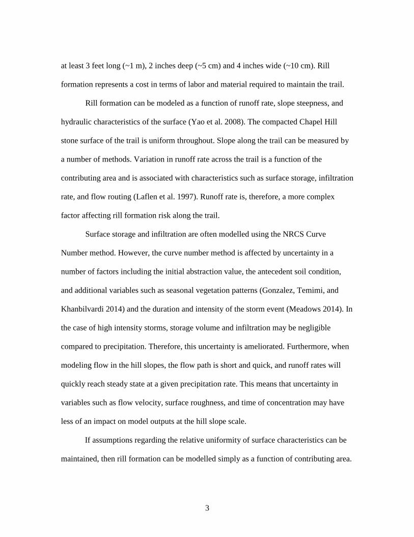
Rill formation can be modeled as a function of runoff rate, slope steepness, and

hydraulic characteristics of the surface (Yao et al. 2008). The compacted Chapel Hill

stone surface of the trail is uniform throughout. Slope along the trail can be measured by

a number of methods. Variation in runoff rate across the trail is a function of the

contributing area and is associated with characteristics such as surface storage, infiltration

rate, and flow routing (Laflen et al. 1997). Runoff rate is, therefore, a more complex

factor affecting rill formation risk along the trail.

Surface storage and infiltration are often modelled using the NRCS Curve

Number method. However, the curve number method is affected by uncertainty in a

number of factors including the initial abstraction value, the antecedent soil condition,

and additional variables such as seasonal vegetation patterns (Gonzalez, Temimi, and

Khanbilvardi 2014) and the duration and intensity of the storm event (Meadows 2014). In

the case of high intensity storms, storage volume and infiltration may be negligible

compared to precipitation. Therefore, this uncertainty is ameliorated. Furthermore, when

modeling flow in the hill slopes, the flow path is short and quick, and runoff rates will

quickly reach steady state at a given precipitation rate. This means that uncertainty in

variables such as flow velocity, surface roughness, and time of concentration may have

less of an impact on model outputs at the hill slope scale.

If assumptions regarding the relative uniformity of surface characteristics can be

maintained, then rill formation can be modelled simply as a function of contributing area.

4

Contributing area can be estimated by various algorithms applied to elevation datasets. In

this case, distinct observations of rill formation can be used to calibrate and compare the

validity of several contributing area algorithms.

The goal of this work is to model rill formation risk along the Natural Heritage

Garden Trail as a function of contributing area. Pursuit of this goal is both directly

applicable to the case of storm water damage at the SCBG and relevant in a broader

context. At the SCBG, design of storm water infrastructure has been based off of the

results of this work. Contributing area is not always readily discerned by on-the-ground

observations, and appropriate modeling and visualization techniques can improve

management and design decisions.

In a broader context, contributing area is a central design parameter for a number

of Best Management Practices (BMPs) and Low Impact Development (LID) strategies.

Recently, the elevation data available in South Carolina has been dramatically improved

by Light Detection and Ranging (LiDAR) derived datasets (SCDNR 2014). These public

datasets can be used to inform landscape design and management – but robust methods

should be identified to transform raw data in to outputs useful for stakeholders.

The methods developed in this work are also applicable in related hydrological

studies, specifically in the delineation of contributing areas. The importance of automated

watershed extraction has been discussed for ecological risk management and planning

(Mantelli, Barbosa, and Bitencourt 2011).

A variety of opportunities for improved management of urban storm water runoff

have been discussed recently in the literature (Burns et al. 2012; Barbosa, Fernandes, and

5

David 2012; Fletcher, Vietz, and Walsh 2014; Fletcher, Andrieu, and Hamel 2013;

Walsh, Fletcher, and Burns 2012). Sustainable management requires optimization in

economic, social, and ecological terms. Runoff can be understood as a resource for

irrigation, or other uses. Society can potentially derive aesthetic, recreational and

educational value from urban streams restored to more natural flow paradigms.

Furthermore, the benefits of sound management practices extend downstream by

decreasing concentrations of pollutants and mitigating floods. Infrastructure design can

be informed by an understanding of localized storm water damage risk. Identification of

erosion prone hot-spots is helpful to plan implementation of best management practices

(Saghafian, Meghdadi, and Sima 2014).

The approach taken in this study is to delineate areas which contribute to runoff

along the trail using a high resolution digital elevation model (DEM) derived using

LiDAR technology. Two different contributing area algorithms are applied, and

stochastic Monte Carlo simulation is used to model uncertainty in the DEM. Outputs are

validated with observed rill formation at various scales, and the Receiver Operating

Characteristic (ROC) curves of the algorithms are used to compare performance.

The primary objectives of this study are:

1) Map the trail and rills on to a LiDAR derived DEM

2) Estimate rill formation risk as a function of contributing area along the trail

3) Compare contributing area estimates with actual rill formation along the trail

6

CHAPTER TWO

REVIEW OF LITERATURE

In this chapter, past works are discussed regarding the methods used in this work.

Three sections are presented below: elevation models and pre-processing, stream and

watershed delineation, and error modeling.

Elevation Models and Pre-Processing

Elevation data is "the reference surface for gravitation driven material transportation"

(Oksanen and Sarjakoski 2006), and as such it is fundamental for storm water runoff

modeling. This section will begin with an overview of elevation models including data

collection, formats, sources and derivatives. The resolution of grid DEMs is a key

characteristic in determining the suitability of a DEM for a given analysis on a given

landscape. Thus, he interplay of DEM resolution and landscape characteristics will be

discussed. DEMs often require pre-processing before they can be used for hydrologic

analysis, and this section will end with a discussion of pre-processing techniques.

Data Formats, Collection Methods, Sources, and Derivatives

An elevation model can be defined as a set of points where each point has

coordinates defining its location in three spatial dimensions relative to the other points in

the set (Fisher and Tate 2006). This definition would include, for example, a list of the

peaks of several mountains, including height above sea level, latitude, and longitude.

7

However, such an elevation model would not be sufficient for tasks such as watershed

delineation; a more refined DEM is required.

A raster dataset is composed of regularly spaced cells. The most common format

of raster elevation data is the grid raster, in which each cell is a square of uniform

dimension. In this paper, the term raster refers to a grid raster dataset. Rasters store data

efficiently because the coordinates of each cell are implicitly defined by the extent of the

raster. Furthermore, they can be efficiently handled by well-developed image processing

algorithms (Grayson and Blöschl 2001; Moore, Grayson, and Ladson 1991).

Direct collection of elevation data can be accomplished with a number of tools,

from the rustic A-frame and water levels to theodolites, electronic distance meters, and

automated total stations. However, even with the most advanced tools, the cost of

surveying large areas can be prohibitive with direct methods.

In contrast to direct measurements taken on the ground, remote sensing methods

collect data from a distance with sensors placed in aerial vehicles or satellites. Remote

sensing elevation data collection methods have been widely used. Photogrammetry

involves taking aerial or satellite photographs of the landscape from two different

perspectives, and then using human or artificial depth perception to delineate contours.

The National Elevation Dataset (NED) was collected using photogrammetric techniques,

and it extends across the entire United States (USGS 2014a). The Shuttle Radar

Topography Mission (SRTM) has provided datasets that cover almost the entire globe

(USGS 2010).

8

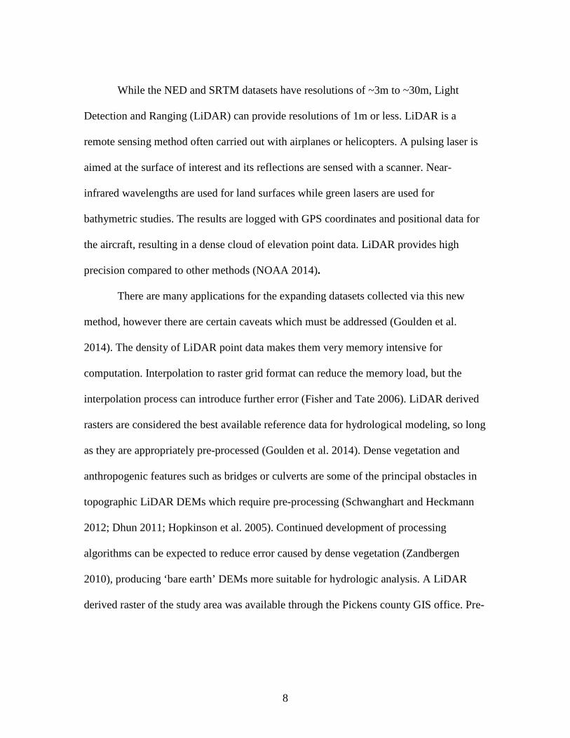
While the NED and SRTM datasets have resolutions of ~3m to ~30m, Light

Detection and Ranging (LiDAR) can provide resolutions of 1m or less. LiDAR is a

remote sensing method often carried out with airplanes or helicopters. A pulsing laser is

aimed at the surface of interest and its reflections are sensed with a scanner. Near-

infrared wavelengths are used for land surfaces while green lasers are used for

bathymetric studies. The results are logged with GPS coordinates and positional data for

the aircraft, resulting in a dense cloud of elevation point data. LiDAR provides high

precision compared to other methods (NOAA 2014).

There are many applications for the expanding datasets collected via this new

method, however there are certain caveats which must be addressed (Goulden et al.

2014). The density of LiDAR point data makes them very memory intensive for

computation. Interpolation to raster grid format can reduce the memory load, but the

interpolation process can introduce further error (Fisher and Tate 2006). LiDAR derived

rasters are considered the best available reference data for hydrological modeling, so long

as they are appropriately pre-processed (Goulden et al. 2014). Dense vegetation and

anthropogenic features such as bridges or culverts are some of the principal obstacles in

topographic LiDAR DEMs which require pre-processing (Schwanghart and Heckmann

2012; Dhun 2011; Hopkinson et al. 2005). Continued development of processing

algorithms can be expected to reduce error caused by dense vegetation (Zandbergen

2010), producing ‘bare earth’ DEMs more suitable for hydrologic analysis. A LiDAR

derived raster of the study area was available through the Pickens county GIS office. Pre-

9

processing the DEM to account for bridges, culverts, and storm drains is discussed later

in this section.

A number of derivatives can be produced from a DEM. Constrained derivatives

such as slope, curvature, or aspect are determined from a fixed neighborhood. Behavior

of constrained derivatives can more readily be described analytically compared to

unconstrained derivatives such as stream and watershed delineation. The behavior of

unconstrained derivatives can vary across multiple scales and requires empirical

characterization (Zandbergen 2011). This is certainly the case for the extraction of

hydrological geomorphological parameters. Stream and watershed delineation will be

discussed in the second bold headed section of this chapter. Empirical characterization of

error in these derivatives is the subject of the third.

Resolution and Landscape Characteristics

For drainage network delineation, higher resolution (~1m) LiDAR DEMs are

preferable to lower resolution photogrammetric DEMs (~10m), especially for accurate

representation of first-order streams (Murphy et al. 2008; Remmel, Todd, and Buttle

2008; James, Watson, and Hansen 2007). Watersheds can be delineated with low

resolution DEMs, but this is dependent on terrain; low relief landscapes in particular

require high accuracy and resolution to reduce uncertainty of drainage patterns (Barber

and Shortridge 2005).

As raster cell size increases, the drainage network becomes more branched,

directly impacting Strahler network properties. To minimize this impact, cell size should

10

ideally be considerably less than the average hill-slope length (Hancock 2005). Another

consideration is that a DEM cannot represent the thalweg of incised channels that are

narrower than the cell size (Garbrecht and Martz 1999). Therefore, precise channel

delineation from the DEM requires that cell size be less than channel width. Otherwise,

stream delineations may tend to unrealistically meander within streambed boundaries,

causing stream length to be overestimated (Goulden et al. 2014).

Interpolation of raster data can be used to artificially increase the resolution of the

raster grid (decrease cell size). The 'Resample' tool (ESRI ) can be used to interpolate

continuous data. Of the available options, cubic convolution has been recommended if

DEM interpolation is the objective (Tarboton and Mohammed 2013) . Cubic convolution

requires more processing time than bilinear interpolation, and it can produce output

values outside the range of input cell values. However, it fits a smooth curve through the

16 nearest input cells (versus 4 nearest inputs for bilinear) which generally provides a

realistic representation of the terrain. Because high resolution data (5x5’ cell size) was

available for the study area, raster interpolation was not used in this work. The stream

channel thalweg was represented using the stream burning technique described in the

next section.

Watershed delineations can vary at different DEM resolutions, and anthropogenic

landscape modifications can add to this variability (Goulden et al. 2014). In addition to

underground storm drains, DEM based hydrological analysis can also be confounded by

ditches which are narrow in comparison to DEM resolution. This can be understood as an

undersampling problem: if more elevation data points are collected, ditches in the surface

11

of the terrain may be better represented. However, increased resolution DEMs requires

greater data storage and processing capacity. Furthermore, underground storm drains

present a challenge for hydrological analysis regardless of DEM resolution. Therefore,

incorporation of relevant anthropogenic features such as storm drains, ditches, or culverts

is an important step in hydrological analysis from DEMs.

DEM Pre-Processing

DEM pre-processing refers to adjustments made to the DEM with the intent of

making it more suitable for subsequent analysis. In the case of stream and watershed

delineation, the DEM is typically pre-processed to remove sinks. The terms sink, pit, and

depression may refer to cells in a DEM which are surrounded by cells of greater

elevation. Sinks may consist of a single cell, or there may be multi-cell sinks. There may

also be nested sinks - sinks within sinks. Flow routing algorithms can be stumped by

sinks, as it is unclear in which direction water flows from them. Sinks may be

representative of real landscape features, or they may be spurious features caused by error

(Vesakoski et al. 2014).

Real sinks in a landscape might include wetlands, salt lakes, retention dams,

sinkholes, or other natural or artificial features. Real sinks can be common in karst

environments or recently glaciated terrain (Zandbergen 2010). Storms can cause some

real sinks to overflow at a breach point. Depending on the hydrological context, it is often

preferable to identify a flow direction which exits the sink to connect with other surface

flows. Very large sinks found in accurate DEMs are likely to represent real landscape

12

features which may require appropriate modeling techniques for derivative processing.

Methods have been developed to assign flow direction through lakes (Maidment 2002).

Sinks may indicate further complications. For example, retention ponds may have

primary and emergency overflow routes which can cause a bifurcation of flow; storm

water drains often connect subsurface pipes and culverts. Detailed hydrological modeling

of real sinks may require each sink to be identified and modeled on a case by case basis.

Artificial or spurious sinks constitute a class of error which is often present in

DEMs before pre-processing. Spurious sinks can result from errors in the input data, the

interpolation technique, rounding or truncation of elevation values, limited resolution and

averaging of values within cells, re-sampling, or reconditioning with linear stream data

(Florinsky 2002; Martz and Garbrecht 1998; Tribe 1992) Spurious sinks have been found

to be more common in areas with low relief in relation to the vertical accuracy of the

DEM (Liang and MaCkay 2000).

Five approaches have been proposed to distinguish between real and spurious

sinks: ground inspection, examination of source data, classification, knowledge-based

and modelling approaches (Lindsay and Creed 2006). While Zandbergen (2010) was

unable to determine area or depth criteria to distinguish between real and spurious sinks

in a DEM, the DEM used had a substantial number of uncorrected underground culverts

(Zandbergen 2010). Distinguishing real and spurious sinks is useful not only for sink

identification and removal, but also for better understanding DEM error in general.

Whether counting total sinks or total sink cells, higher resolution DEMs have

been found to contain higher numbers of sinks, and the sinks tend to be smaller in terms

13

of depth and volume. This trend is explainable by the more accurate representation of

micro-topography in higher resolution DEMs. Single cell sinks have been found to be

predominant, especially in lower resolution DEMs (Vesakoski et al. 2014). LiDAR data

in particular often contains more sinks (Petroselli 2012).

Sinks can be problematic if the DEM is used as input to certain flow routing

algorithms. Sinks disconnect the drainage network, creating interior sub-watersheds with

no outlets. A number of algorithms have been developed to identify sinks in a DEM and

deal with them, spurious or otherwise. Algorithms may fill the sinks by raising sunken

cells to higher elevations or breach the sinks at pour points by lowering elevation values

of specific neighboring cells.

Many sinks are small or even single cell, in which case the various sink removal

algorithms generally give equivalent results. However, some derivative applications will

be more sensitive than others to uncertainty in sinks and sink removal. For example, an

attempt to quantify surface depression storage capacity from a DEM would be heavily

dependent upon accurate sink representation. Sinks located on a watershed boundary

might be of particular interest in watershed delineation and storm water modeling. Filling

expansive, multi-cell sinks effectively reduces the accuracy of the DEM in the filled

areas. The results of an automated breaching algorithm may not reflect the real positions

of culverts or overflows. Therefore, for high resolution stream and watershed delineation,

the application and results of sink removal algorithms should be justified in relation to the

derivative of interest.

Two basic strategies for removing sinks from a DEM are considered: raising the

14

elevation of each sink to its lowest neighbor (filling ), and lowering the elevation of a cell

or cells surrounding the sink.

A number of algorithms can be used to fill depressions. Although their processing

times can vary substantially, they are reported to give equivalent results (Vesakoski et al.

2014). Jenson and Domingue’s algorithm is widely used and available in the ArcGIS

tools (Jenson and Domingue 1988). Wang and Liu’s method has been recently cited due

to its speed and simplicity (Wang and Liu 2006; Ukkonen, Sarjakoski, and Oksanen

2007; Vesakoski et al. 2014).

Filling algorithms raise the elevation in each sink just enough for water to flow

from the processed cell to the edge of the grid. The cell elevation values of a filled DEM

are greater than or equal to the original DEM. Filling is the most widely used approach

(Zandbergen 2010). In areas with low relief, filling algorithms may substantially modify

the input DEM. Also, structures such as bridges can cause ‘digital dams’ in the DEM. If

left uncorrected, filling algorithms will raise and flatten the channel upstream of such

structures, reducing the accuracy of the DEM. This is especially problematic in high

resolution DEMs – the increased precision caused by smaller cell size can increase errors

if small structures such as bridges are represented as the land surface in the DEM

(Goulden et al. 2014).

The main alternative to filling is to remove sinks by decreasing the elevation

values of cells along a designated flow path, known as 'breaching' or 'burning.' Stream

burning was first developed to enforce drainage along known stream channels which

were not represented in the raw DEM. Breaching techniques have been developed more

15

recently to account for ditches, culverts, and storm drains (Dhun 2011). Unlike most

filling algorithms, the results of various breaching and burning algorithms can vary

widely with operational parameters such as depth, width and length of the breach

modification to the DEM.

The general function of breaching algorithms, after identifying each sink, is to

search for a cell of lower elevation within a given range, and then decrease the elevation

of cells between the sink and the lower cell. To prevent the breaching algorithm from

causing too much alteration to the DEM, constrained breaching limits the breach length

to a number of cells (Martz and Garbrecht 1999). Dhun developed an automated

breaching algorithm for routing flow through obstructions such as roads and bridges

(Dhun 2011).

While the breaching techniques discussed above lower only certain cells

surrounding sinks, stream burning lowers all of the cells which correspond to streams.

These techniques can improve stream and watershed delineation results in low relief

areas, but substantial modification of the DEM may not be appropriate in all cases.

The hydrography vector dataset used to burn the DEM should be a fully dendritic

network consisting of a unique flow line for each stream reach. Shorelines of lakes, wide

rivers, and oceans should be removed. If the D8 flow direction method (discussed in the

next section) is used, then stream bifurcation is not allowed. Hydrographic features of

adjacent watersheds should also be burnt in to the DEM, so that subsequent watershed

delineation will not be unduly biased in favor of the burnt watershed. Finally, and

perhaps most important, the resolution of the hydrography data and the DEM should be

16

approximately equal. If the DEM is of significantly coarser resolution than the vectors to

be burnt, a number of errors can result (Saunders 1999).

One error which can occur even if the above considerations are taken in to

account is extraneous parallel streams in the output. If the vector lines are offset from the

channels present in the raw DEM by more than a few pixels, then streams might be

delineated in both the burnt channels and the raw channels (which actually represent a

single stream). A method to reduce this error is to augment the burnt stream with a buffer

in which cells are raised or lowered to slope gently to the burnt stream. This creates a

streambed with a channel inside it, mimicking typical landscapes (Hellweger 1997).

Another problem with the basic stream burning method is that a very deep burn

can alter adjacent watershed boundaries. Normalized stream burning is an improved

technique designed to address this issue. Instead of burning cells to an arbitrary depth,

each burn cell is lowered based on a function of surrounding terrain. Normalized stream

burning can be used in conjunction with streambed buffering and has been shown to be

an effective technique for improving the accuracy of automated watershed delineation

(Baker, Weller, and Jordan 2006).

Burning can also be used for stream and watershed delineation in areas with

underground culverts or bridges crossing the flow path. If the locations of culverts are

known and represented in the GIS, then they can be burnt in to the DEM used as input to

the flow direction procedure. Recently, Goulden et al (2014) found a significant error in

watershed delineation when a raised road surface obstructed the natural flow. A culvert

crossed beneath the road, and when it was burnt into the DEM, they were able to

17

delineate a more accurate watershed. Interestingly, since the width of the roadbed was 8

m, course resolution DEMs (>10 m) did not require correction for the culvert because

they did not represent the road distinctly. These results have been replicated (Li et al.

2013). It follows that precise application of stream burning at bridges and culverts may

only be necessary in higher resolution DEMs, as smaller bridges and embankments are

less likely to be represented in low resolution DEMs.

It should be noted that simply burning culverts in to the DEM may not be

appropriate in all cases. For example, in areas with extensive underground drainage

networks but only limited inlets to the network, gap flow should also be represented. Gap

flow is surface flow which exceeds the capacity or otherwise does not enter the artificial

drainage network. It might be necessary, in that situation, to develop multiple flow

direction representations for both surface and subsurface flow (Pourali et al. 2014).

Unlike hydrography data, which is available for the entire United States in a

uniform format from the US Geological Survey (USGS 2014b), storm water

infrastructure data is not generally readily available. Field surveys are costly, but

sometimes necessary to collect the data. Some municipalities and institutions maintain

CAD files of infrastructure, and this data can be incorporated in to the GIS. A pre-

processing step for vector data imported from CAD to a GIS is to buffer the CAD lines

by a very small distance (i.e. .25 cm) and dissolve around the buffer, resulting in a single

thin polygon which describes multiple polylines and loads much faster (Baumann 2014).

In this section elevation data and pre-processing steps were reviewed. Elevation

data comes in a variety of formats depending on the collection method and the source.

18

LiDAR datasets represent the highest quality currently attainable in a cost-effective

manner for wide extents. However, LiDAR derived DEMs often require pre-processing

for hydrologic analysis to reduce error associated with sinks and infrastructure. A variety

of pre-processing algorithms have been developed. The general workflow is to breach

impoundments cause by 'digital dams' and subsequently fill any remaining small sinks.

Once a DEM is pre-processed, automated stream and watershed delineation is possible.

Stream and Watershed Delineation

Stream and watershed delineation are fundamental steps in hydrologic analysis.

The basic questions which delineation begins to answer are 'Which way?' and 'How

much?' With a pre-processed DEM as input, the first step in delineation is determination

of flow direction. Also known as flow routing algorithms, a variety of methods exist for

this task. Two more commonly used flow routing algorithms are the D8 and D-infinity

methods. These methods are somewhat complementary as they are best applied on

channels and hill slopes, respectively. Once flow directions are determined, watersheds

can be delineated.

The next step is stream definition. While the National Hydrography Dataset

(USGS 2014b) is based on field observation, automated stream delineation in a GIS is

typically based on some threshold of contributing area. Determination of the contributing

area threshold may be accomplished through several techniques discussed in the second

subsection.

19

Flow Direction Algorithms

Flow direction or flow routing algorithms are central to automated stream and

watershed delineation. When using raster format DEMs as input, the typical method for

calculating flow direction is the D8 algorithm (O'Callaghan and Mark 1984). The D8

algorithm is straightforward and efficient, but it has certain drawbacks. The D-infinity

algorithm is an alternative and complementary method (Tarboton 1997).

After pre-processing, every cell in a DEM has at least one neighboring cell of

lower elevation, with the following exceptions: cells on the edge of the raster, and

remaining sinks. Cells in the top and bottom rows and leftmost and rightmost columns

are generally not assigned a flow direction value. Cells located on the edge of the raster

which are lower than all of their neighboring cells are pour points where runoff likely

flows beyond the extent of the DEM. Another set of exceptions is sinks which have been

left after pre-processing. These would require consideration on a case-by-case basis.

Examples include storm drain inlets, lakes, or artificial basins (Tarboton and Ames 2001).

Aside from the aforementioned exceptions, the D8 algorithm assigns a flow

direction value to each cell based on the location of its lowest neighboring cell. In a grid

raster, each cell is surrounded by eight neighbors; the flow direction value assigned to the

cell corresponds to the relative location of its lowest neighbor. A single cell may have

inflow from multiple neighbors, but the D8 method will assign its outflow to one and

only one neighbor. Thus, there are eight possible directions in which flow may be routed

from a single cell, as shown in Figure 1 below (adapted from (Maidment 2002).

20

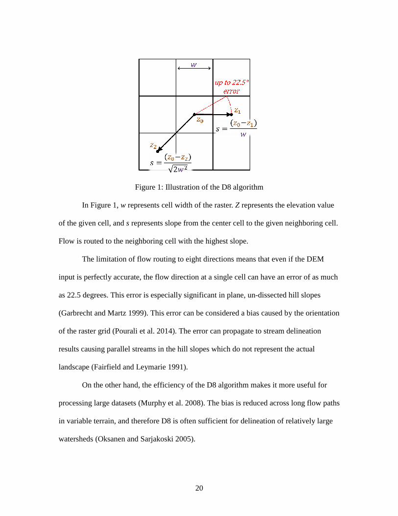
Figure 1: Illustration of the D8 algorithm

In Figure 1, w represents cell width of the raster. Z represents the elevation value

of the given cell, and s represents slope from the center cell to the given neighboring cell.

Flow is routed to the neighboring cell with the highest slope.

The limitation of flow routing to eight directions means that even if the DEM

input is perfectly accurate, the flow direction at a single cell can have an error of as much

as 22.5 degrees. This error is especially significant in plane, un-dissected hill slopes

(Garbrecht and Martz 1999). This error can be considered a bias caused by the orientation

of the raster grid (Pourali et al. 2014). The error can propagate to stream delineation

results causing parallel streams in the hill slopes which do not represent the actual

landscape (Fairfield and Leymarie 1991).

On the other hand, the efficiency of the D8 algorithm makes it more useful for

processing large datasets (Murphy et al. 2008). The bias is reduced across long flow paths

in variable terrain, and therefore D8 is often sufficient for delineation of relatively large

watersheds (Oksanen and Sarjakoski 2005).

21

Various flow routing algorithms generally produce similar results in convergent

topography such as around streams. However, the results may vary significantly in

divergent terrain such as on hillslopes (Lindsay 2006). For the purpose of modeling

stormwater runoff at a fine scale, a more sophisticated algorithm is desirable.

The D-infinity flow routing algorithm performs well in divergent terrain and takes

raster format DEMs as input (Tarboton 1997). The D-infinity algorithm allows for

outflow from a single cell to be divided between multiple neighboring cells according to

their relative steepness. Thus, instead of limiting the flow to one of eight possible

directions, D-infinity effectively routes flow at any angle from the cell. Furthermore the

D-infinity algorithm is capable of representing braided stream networks. D-infinity

compares well with other multiple direction flow routing algorithms. It has been used to

represent flow on hill slopes in conjunction with the D8 algorithm in streams (Grimaldi et

al. 2010). Although more complex than the D8 algorithm, the D-infinity algorithm is not

overly complicated. It is illustrated in figure 2 below.

22

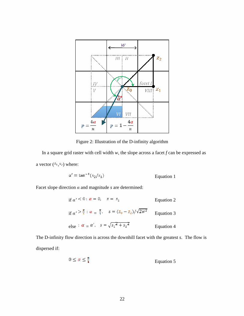
Figure 2: Illustration of the D-infinity algorithm

In a square grid raster with cell width w, the slope across a facet f can be expressed as

a vector ( , ) where:

Equation 1

Facet slope direction α and magnitude s are determined:

if α’ Equation 2

if α’ = Equation 3

else = Equation 4

The D-infinity flow direction is across the downhill facet with the greatest s. The flow is

dispersed if:

Equation 5

23

Facet angle α can be used to determine the portion of flow p to opposite and adjacent

cells. The D-infinity flow direction r’ is a function of α and facet position f.I-f.VIII .

(Tarboton 1997)

Flow Accumulation & Stream Definition

Once the flow from every cell has been routed appropriately, the flow

accumulation can be calculated. Flow accumulation can be calculated in a straightforward

manner on the basis of area, or it can be weighted according to surface parameters such

as permeability or infiltration rate. Streams are commonly delineated using a flow

accumulation threshold. Determination of the threshold should take in to account the

terrain and environmental variables as well as the purpose of the analysis (James, Watson,

and Hansen 2007).

The simplest flow accumulation algorithms simply add up the number of cells

which flow in to each cell. The headwaters of first order streams are then designated

based on a stream definition threshold or critical source area. Whereas stream definition

threshold may be in units of cells, the critical source area is the number of cells

multiplied by the area of each cell. Both concepts describe a threshold by which streams

are determined. Maidment (2002) has suggested using a relative threshold of 1% of the

maximum flow accumulation value in the raster as the stream definition threshold.

Alternatively, an absolute threshold of 5,000 m2 has been used (Lindsay and Evans

2008). These determinations are apparently made based on experience: field observations

and comparison of derived stream networks with actual stream networks.

24

In reality, the headwaters of 1st order stream channels vary randomly and

systematically (Garbrecht and Martz 1999). Modeling random variation will be discussed

in the third section of this work. Systematic variation can be modeled with empirical

weights such as curve numbers, process models such as GeoWEPP (Renschler 2003), or

based on an analysis of the terrain (Tarboton and Ames 2001).

Curve numbers can be assigned based on factors such as land cover and soil type

allowing for total runoff to be estimated from a given rain event (Blair et al. 2014). The

NRCS curve number method is widely used and can be modified based on slope (Huang

et al. 2006), or season (Gonzalez, Temimi, and Khanbilvardi 2014). Assignment of curve

numbers provides one means of weighting flow accumulation from each cell with an

estimated runoff volume. Estimated runoff volume can then be used as the threshold

metric to define the stream network.

DEM Error Propagation and Modeling

DEM quality studies have been divided into categories (Oksanen and Sarjakoski

2006). The earliest studies aim to define DEM accuracy. More recent studies concern

error propagation, characterization of DEM error through empirical semi-variogram

analysis, and application-specific error models including other relevant datasets. DEMs

and their derivatives are fundamental data inputs for a variety of applications.

Application-specific error models are enabled by better understanding of DEM accuracy

and characteristics of DEM error. DEM error propagation analysis is based on the proper

spatial characterization of error, and while the analysis may rely on analytical or

25

numerical methods, an appropriately defined error model can be used in either

methodology (Oksanen and Sarjakoski 2006).

The derivatives of interest are delineations of a small watersheds and concentrated

surface flows, for application in fine-resolution storm water damage prediction. In this

section the following topics are reviewed: characterizations of DEM error; error

propagation from DEM to stream and watershed delineation; and stochastic, Monte Carlo

methods of error modelling.

Typology of DEM Error

DEM error is difficult to quantify. It is hard to identify how much of the data

deviates from the true surface, and by how much. The error curve characteristically has

extreme outliers, possibly due to systematic errors in data collection and processing.

While it is accepted that DEM error is spatially auto-correlated, it is unclear whether

there are other spatial correlations (Lindsay and Evans 2008).

Perhaps the best way to approach the subject is to begin with a qualitative

characterization of DEM error. One characterization is between systematic, gross, and

random error (Fisher and Tate 2006). Systematic error is caused by a deterministic bias in

the collection or processing of data. If systematic error is discovered, it can often be

analyzed and represented by a function (Thapa and Bossler 1992). One example of

systematic error is the presence of 'ghost contours' in raster DEMs derived from contour

maps. The contour lines are oversampled relative to the areas between contours, causing

26

bias in the DEM. A graph of elevation value by cell count will reveal periodic peaks at

the contour intervals (Fisher and Tate 2006).

Another example of systematic error which can be found in LiDAR DEMs is an

upward bias in wetland vegetation land cover (Hopkinson et al. 2005). Any canopy cover

can reflect LiDAR signal, causing an upward bias if the desired value is the earth.

However, if the LiDAR data is collected in leaf-off conditions, then some data points will

be more likely to represent the ground surface. In that case, appropriate filtering

techniques can remove the canopy data to produce a bare-earth DEM. Ground surface

which is covered with water and obscured by canopy is especially problematic - water

causes the signal to disperse, making filtering more difficult, and leading to an upward

bias (Hopkinson et al. 2005).

A third example of systematic error in the context of hydrologic modeling with

high resolution DEMs, already discussed in section 1 above, is the representation of

bridges and other structures as obstructions to surface flow. Given data on the location of

such structures, it is possible to reduce or eliminate this error through pre-processing.

Gross errors, also known as blunders, are the result of failures of equipment or

users to properly collect the data. Some data sources may be more likely to provide gross

errors than others, as quality control meaures may differ. Modelling of gross errors is

especially difficult (Wise 1998). An example of gross errors in DEMs derived from

digitization of printed maps is deformation of the printed media (Florinsky 1998). Finally

there are random variations around the true reference value. In the absence of systematic

27

and gross error, random error is readily modelled with stochastic simulations (Oksanen

and Sarjakoski 2006).

Fisher and Tate (2006) discuss another way of classifying error as stemming from

data generation, data processing and interpolation, or differences between the scale of

relevant terrain features and the scale of the DEM.

Data generation method, processing method, and grid size have been found to

effect derivative outputs of the DEM, such as the location and size of sinks (Vesakoski et

al. 2014). This classification can alternatively be described as data based error, model

based error, and model based uncertainty, respectively. This suggests an additional class -

data based uncertainty.

This classification can also be illustrated with examples described previously.

Equipment malfunction would be a data generation error. Ghost contours would be a

model based error. The inability of a grid DEM to represent an incised channel narrower

than the DEM cell size would be model uncertainty. The effect of vegetation, buildings,

and water in obscuring or diffusing the LiDAR signal would be data based uncertainty.

(Christian et al. 2013) further subdivide data based uncertainty into epistemic and

aleatory classes. Epistemic uncertainty is reduced by better data collection methods (Liu

and Gupta 2007), while aleatory uncertainty is found in parameters that naturally vary

due to random processes - no amount of data collection can eliminate aleatory

uncertainty. Elevation values around an active volcano might demonstrate aleatory

uncertainty caused by unpredictable subsidence and uplifting of the earth’s crust

28

Using a LiDAR data as the reference, Oksanen and Sarjakoski (2006) found that

average slope, standard deviation of curvature, and vegetation index were the terrain

attributes with the highest correlations with semivariogram parameters of a Fine Scale

Topo dataset. This apparently corresponds with previous work which identified similar

terrain attributes expected to influence the quality of DEMs produced from automated

photogrammetry or active systems such as LiDAR: sloping ground, which may alter

signal reflection; microrelief causing measurement points to be spatially

unrepresentative; non-selective sampling by the sensor; land cover with varying

reflectivity (Lemmens 1999).

Error Propagation

If the various kinds of DEM error comprise complications for analysis, the

propagation of DEM error to derivative outputs adds complexity to the situation. For

analyses requiring multiple input datasets, DEM error comprises only one kind of error

which can affect the validity of model output. In those cases, the uncertainty and error

from each input dataset should be recognized and dealt with appropriately so that the

significance of model output can be understood. Watershed delineation requires two

kinds of data: the DEM, and any infrastructure which may direct flow paths in ways that

the DEM does not represent (also, it is possible that natural geologic features may direct

subsurface flows in ways that effect the watershed delineation, but this is not likely to be

a major factor at the SCBG). Estimation of runoff volume would require precipitation

data and additional data if infiltration, storage, or other processes are to be represented.

29

Estimation of flow velocity would require surface roughness coefficients and flow depth,

in addition to slope which may be derived from the DEM. Just as scientific calculations

must keep track of significant figures and confidence intervals, geospatial analyses must

account for any error inherent in each of the data inputs.

Furthermore, model parameters, even if properly calibrated, likely bring in some

amount of error. The model itself can only describe a subset of the processes taking place

in reality, and validation is crucial before a model can be applied with any reliability.

Continued refinement and validation of the mathematical models and assumptions can

increase confidence in the outputs (Christian et al. 2013).

In stream and watershed delineation, error propagates from the DEM in a rather

predictable manner: the greatest uncertainty is found at the stream channel heads and in

areas of low relief (Petroselli 2012; Zandbergen 2011; Goulden et al. 2014). This trend

can be understood in terms of a ratio (Gyasi‐Agyei, Willgoose, and De Troch 1995). The

numerator term is the average change in elevation from each cell to its lowest neighbor,

the 'drop'; the denominator is the vertical precision of the raster. Only if this ratio is

greater than unity, then the DEM is suitable for hydrological modelling. It should be

noted that the Gyasi-Agyei suitability ratio can be expressed as a local variable, meaning

some parts of a DEM may be suitable while other areas are not (Goulden et al. 2014).

Comparing the results of a Monte Carlo technique described below with a number

of independent manual delineations, Oksaken and Sarjakoski (2005) found it possible to

classify lengths of watershed delineations into three groups: sharp, diffuse, and alternate.

Sharply delineated areas are areas with little uncertainty concerning the direction of

30

overland water flow. Diffuse delineations indicate that there is a wide spread area where

the water flows in one of multiple possible directions. Alternate delineations occur in

areas where the watershed border is located in one of several distinct places. This

classification scheme allows for a better understanding of error propagation in watershed

delineation.

Oksanen and Sarjakoski (2005) also found that with a grid size of 10m and a

RMSE < 5.0m watershed size could reliably be reported only to the precision of 0.1 sq

km, or +/- ~500 grid cells. They found that the percent error of watershed area was up to

24% for the basins of first order streams (about 1km2 area). It is expected that these

statistics will vary in different datasets of different landscapes. The RMSE and average

drop may be considered key factors in the uncertainty of watershed delineation.

Error Modeling

The application of statistically based confidence intervals for delineation is

limited by technical complexity and resistance to unfamiliar models (Christian et al.

2013). Stochastic analyses provide an alternative to incorporate uncertainty and provide

useful results. Zandbergen (2011) has listed the following applications of stochastic

Monte Carlo simulation of random errors in DEMs: feature extraction, flow path

direction, drainage basin delineation, route optimization, roughness, flow accumulation,

curvature, and slope failure.

31

Stochastic Monte Carlo simulation can be considered a 'brute force' technique

which has been successfully applied to evaluate uncertainty due to error propagation from

elevation data to watershed delineation (Oksanen and Sarjakoski 2006). While it is

computationally demanding, distributed computational methods have been presented to

reduce processing time for Monte Carlo watershed delineations (Ukkonen, Sarjakoski,

and Oksanen 2007).

Wechsler (2000) listed four assumptions of stochastic simulation of error in

terrain analysis, restated by Lindsay and Evans (2008) as follows:

(1) DEM error exists and constitutes uncertainty that is propagated with the

manipulation of terrain data;

(2) The exact nature of these errors is unknown;

(3) DEM error can be represented by a distribution of topographic realizations;

(4) The true surface lies somewhere within this distribution of surfaces

Key parameters for the simulation include the error distribution function, the range of

spatial autocorrelation of the error, and the number of repetitions (Oksanen and

Sarjakoski 2005). It is commonly assumed that the error is distributed according to a

Gaussian function. Empirical studies have actually found a high amount of extreme

outliers, so the Gaussian function may not accurately represent the true error distribution.

However, it is adequate to give qualitative results concerning uncertainty in the output.

32

Histogram matching is a technique which can be used if the error distribution cannot be

adequately approximated by a Gaussian distribution (Lindsay and Evans 2008).

Assumptions can be made to simplify the error distribution function. The mean of

the error function is commonly set at zero, which assumes that there is neither a net

upward nor downward bias to the elevation data. The root-mean-square error (RMSE) of

the elevation dataset can be used as an estimate of the standard deviation of the error

function (Gatziolis and Fried 2004).

Various techniques have been used to model spatial autocorrelation in the

simulated error (Lindsay and Evans 2008). Spatial moving averages using a low pass

filter is computationally efficient, an important consideration when the process will be

iterated many times over (Oksanen and Sarjakoski 2005). Regardless of the method for

achieving spatial autocorrelation, the range of spatial autocorrelation is an important

consideration. One study found three distinct 'frequencies' of error: low, medium, and

high, in photogrammetric DEMs compared to LiDAR. Low frequency error, spatially

autocorrelated at a range of 30 to over 100 cell widths (in a 10m cell size DEM) appeared

independent of terrain attributes, possibly resulting from errors in stereo-plotting.

Medium frequency error was mostly attributable to systematic error in the contour data.

High frequency error, with a spatial autocorrelation range of 1-2 cell widths was

correlated with slope (Oksanen and Sarjakoski 2006).

The complexity of simultaneously modeling three frequencies of error is

compounded by the potential for non-stationarity of the error function. That is, empirical

assessments have found that the error distribution is better modelled by a set of functions

33

which vary by region. Not only does the error vary, but the function which describes the

error distribution also varies. Simplification of the error distribution function to only

model high frequency errors may be an appropriate shortcut for constrained, local

derivatives such as slope and aspect, but is not considered appropriate for drainage basin

delineation (Oksanen and Sarjakoski 2006).

However, there are key differences between the cited work and that which is

proposed. Namely, the error distribution in a LiDAR dataset (cell size ~5ft) may have

different characteristics. In fact, LiDAR error has been described as mostly consisting of

white noise, or speckle: high frequency error (Dhun 2011). Furthermore, the size of the

drainage basins delineated by Oksanen and Sarjakoski is several orders of magnitude

larger than the size of the contributing areas which cause rill formation. In the scale of

their analysis, the drainage basins of interest here could almost be considered local

derivatives.

Finally, the number of times the Monte Carlo simulation is repeated is an

important parameter that must be considered. Some studies have found that the results

were still unstable after running 100 to 1000 simulations (Heuvelink 1998).Other studies

have found 500 to 2000 simulations to be sufficient (Lindsay and Evans 2008; Oksanen

and Sarjakoski 2005). The necessary number of simulations will ultimately be dependent

on characteristics of the dataset and the derivatives of interest. For robust results, the

stopping condition can be based on convergence - the stability of the frequency

distribution of the results. (Zandbergen 2010; Lindsay and Evans 2008).

34

This review has discussed the fundamentals of digital elevation model datasets

including collection methods, formats, and uses. Methods use to estimate contributing

areas have been discussed. Stochastic Monte Carlo error simulation has been reviewed

for the purpose of describing the uncertainty in watershed delineation.

35

CHAPTER THREE

MATERIALS AND METHODS

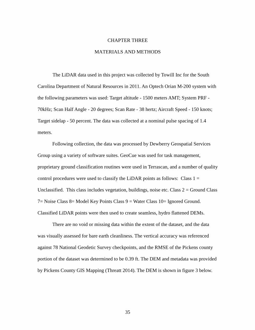
The LiDAR data used in this project was collected by Towill Inc for the South

Carolina Department of Natural Resources in 2011. An Optech Orian M-200 system with

the following parameters was used: Target altitude - 1500 meters AMT; System PRF -

70kHz; Scan Half Angle - 20 degrees; Scan Rate - 38 hertz; Aircraft Speed - 150 knots;

Target sidelap - 50 percent. The data was collected at a nominal pulse spacing of 1.4

meters.

Following collection, the data was processed by Dewberry Geospatial Services

Group using a variety of software suites. GeoCue was used for task management,

proprietary ground classification routines were used in Terrascan, and a number of quality

control procedures were used to classify the LiDAR points as follows: Class 1 =

Unclassified. This class includes vegetation, buildings, noise etc. Class 2 = Ground Class

7= Noise Class 8= Model Key Points Class 9 = Water Class 10= Ignored Ground.

Classified LiDAR points were then used to create seamless, hydro flattened DEMs.

There are no void or missing data within the extent of the dataset, and the data

was visually assessed for bare earth cleanliness. The vertical accuracy was referenced

against 78 National Geodetic Survey checkpoints, and the RMSE of the Pickens county

portion of the dataset was determined to be 0.39 ft. The DEM and metadata was provided

by Pickens County GIS Mapping (Threatt 2014). The DEM is shown in figure 3 below.

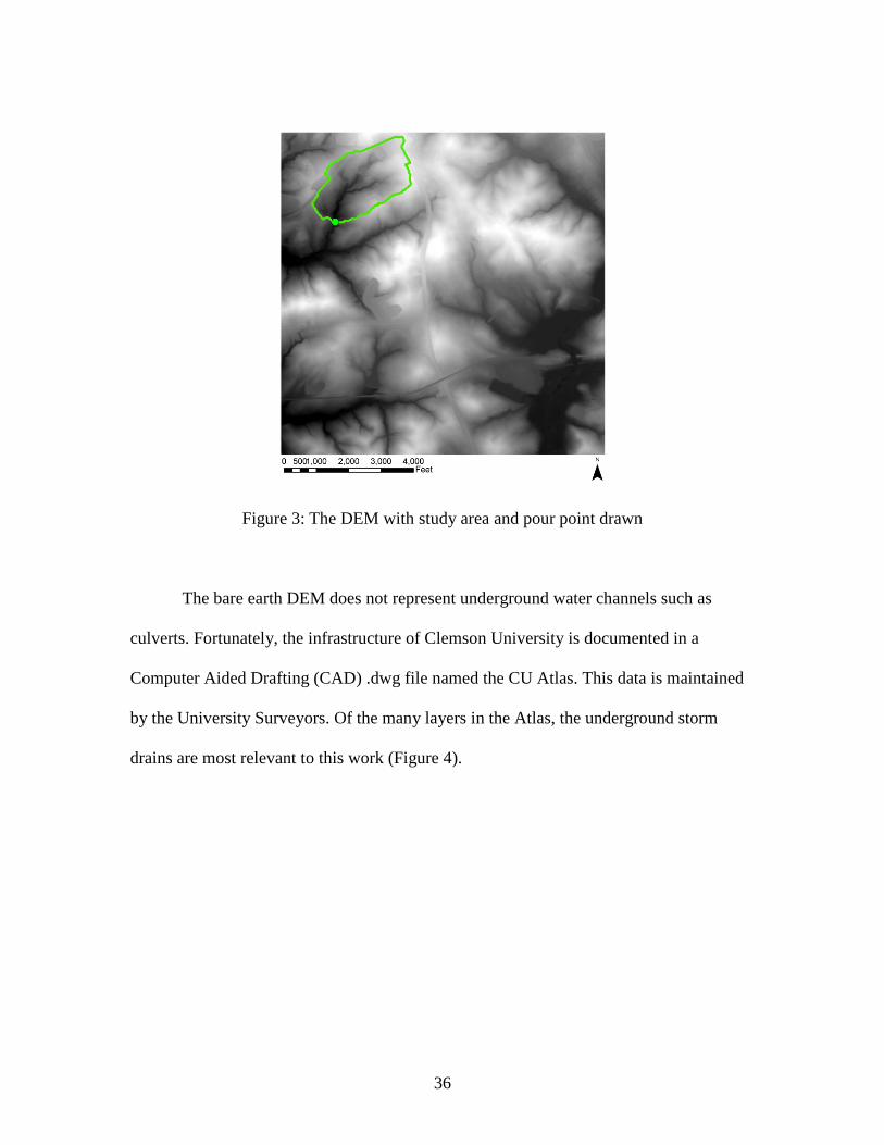
36

Figure 3: The DEM with study area and pour point drawn

The bare earth DEM does not represent underground water channels such as

culverts. Fortunately, the infrastructure of Clemson University is documented in a

Computer Aided Drafting (CAD) .dwg file named the CU Atlas. This data is maintained

by the University Surveyors. Of the many layers in the Atlas, the underground storm

drains are most relevant to this work (Figure 4).

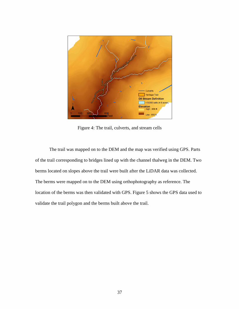
37

Figure 4: The trail, culverts, and stream cells

The trail was mapped on to the DEM and the map was verified using GPS. Parts

of the trail corresponding to bridges lined up with the channel thalweg in the DEM. Two

berms located on slopes above the trail were built after the LiDAR data was collected.

The berms were mapped on to the DEM using orthophotography as reference. The

location of the berms was then validated with GPS. Figure 5 shows the GPS data used to

validate the trail polygon and the berms built above the trail.

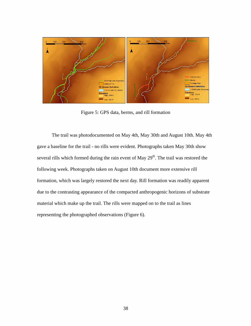
38

Figure 5: GPS data, berms, and rill formation

The trail was photodocumented on May 4th, May 30th and August 10th. May 4th

gave a baseline for the trail - no rills were evident. Photographs taken May 30th show

several rills which formed during the rain event of May 29th. The trail was restored the

following week. Photographs taken on August 10th document more extensive rill

formation, which was largely restored the next day. Rill formation was readily apparent

due to the contrasting appearance of the compacted anthropogenic horizons of substrate

material which make up the trail. The rills were mapped on to the trail as lines

representing the photographed observations (Figure 6).

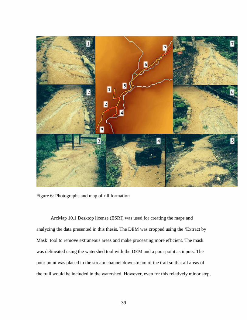
39

Figure 6: Photographs and map of rill formation

ArcMap 10.1 Desktop license (ESRI) was used for creating the maps and

analyzing the data presented in this thesis. The DEM was cropped using the ‘Extract by

Mask’ tool to remove extraneous areas and make processing more efficient. The mask

was delineated using the watershed tool with the DEM and a pour point as inputs. The

pour point was placed in the stream channel downstream of the trail so that all areas of

the trail would be included in the watershed. However, even for this relatively minor step,

40

some pre-processing was found to be necessary. The ‘Fill’ tool must be used on the DEM

to remove sinks. The watershed delineation workflow consist of the following tools:

‘Flow Direction’, ‘Flow Accumulation’, ‘Snap Pour Point’, and ‘Watershed’ (Maidment

2002). The watershed was delineated using the filled DEM, however, some areas of the

watershed were not included in the output. These errors of omission were caused by the

inability of the raw LiDAR DEM to model underground storm drains. Therefore,

underground storm drains, represented as vectors in the CU Atlas were used to lower

corresponding cells in the DEM by three feet before removing sinks and completing the

watershed delineation workflow. The ‘Raster Calculator’ tool was used to make the storm

drain adjustment; the ArcHydro 'Burn Stream Slope' tool was not suitable due to its effect

of increasing the elevation values of cells untouched by the stream (or in this case storm

drain) vectors. The raster output of the watershed tool was converted to a polygon

representing the area which drains to the pour point. This polygon was used to crop the

DEM to the Area of Interest, thereby reducing processing time required for subsequent

analysis.

Two areas upslope of the trail had been substantially modified to divert storm

water with berms. These modifications took place after the LiDAR data was collected,

therefore they were not included in the LiDAR DEM. Even if the earthworks had been in

place for LiDAR data collection, it is possible that the resolution of the LiDAR would not

be sufficient to accurately represent them. The earthworks were mapped on to the DEM

using the orthophoto and ground observations of the earthworks. The berms were

represented as line features, and cells in the DEM which corresponded to the berm lines

41

were raised 2 feet in elevation. These adjustments were also made using the ‘Raster

Calculator’ tool.

The DEM was also adjusted to represent the stream channel by lowering

corresponding cells 1 foot. The stream channel was determined using the D8 flow

direction and flow accumulation algorithms. The stream channel was defined as cells

with a contributing area estimated to be greater than 8,000 cells (200,000 square feet, or

about 4.6 acres). This stream definition threshold was determined based on observation of

the study area. The stream channel adjustment was done to reduce the tendency of the

Monte Carlo simulations to spread flows out within the flood plain. While a spread out

flow model can be informative for flood mapping, the objective of this study is to model

rill formation. The stream generally stayed within its banks during the study period; it

only crosses the path under bridges; and what flooding did occur caused minimal damage

to the trail during the study period.

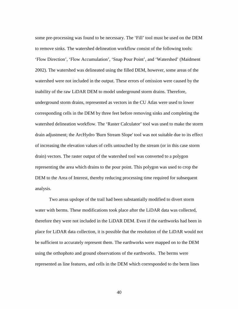
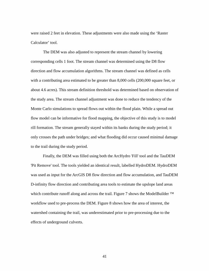
Finally, the DEM was filled using both the ArcHydro 'Fill' tool and the TauDEM

'Pit Remove' tool. The tools yielded an identical result, labelled HydroDEM. HydroDEM

was used as input for the ArcGIS D8 flow direction and flow accumulation, and TauDEM

D-infinity flow direction and contributing area tools to estimate the upslope land areas

which contribute runoff along and across the trail. Figure 7 shows the ModelBuilder ™

workflow used to pre-process the DEM. Figure 8 shows how the area of interest, the

watershed containing the trail, was underestimated prior to pre-processing due to the

effects of underground culverts.

42

Figure 7: DEM Pre-Processing developed in ModelBuilder ™

Figure 8: Pre-processing affects the AOI delineation

43

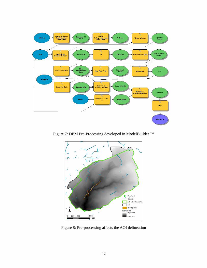
Rill lines were buffered by 5 feet and used to divide the trail polygon in to two

non-overlapping sets of polygons: areas affected by rill formation and areas unaffected by

rills (Figure 9). This binary division of the trail was used to validate the algorithm output

and create the Receiver Operator Characteristic (ROC) curves detailed below.

Figure 9: Creating the trail and rill polygons

Contributing area along the trail was estimated in four ways. Two algorithms

were used: D8 and D-infinity. Each algorithm was run once on the HydroDEM and then

again as part of a Monte Carlo simulation of error in the DEM. To run the basic

algorithms, the flow direction tool is first used, followed by flow accumulation or

contributing area. For the D8 algorithm, the Flow Direction and Flow Accumulation

tools, part of the Spatial Analyst extension of ESRI ArcMap were used. The D-infinity

algorithm was downloaded as part of the TauDEM package (Tarboton and Mohammed

2013). TauDEM is free to download and can be run independently or as part of ArcMap.

The relevant tools are called D-infinity Flow Direction and D-infinity Contributing Area.

The Monte Carlo technique was implemented using the Python programming

language to create 1,000 elevation simulations. In each simulation, a raster of normally

44

distributed values is created. This raster represents random noise in the DEM, and it is set

to the same cell size and extent as the input DEM. It is spatially autocorrelated, or

smoothed, by using Focal Statistics at a radius of 5 ft (1 cell width). Then, map algebra is

used to adjust the values of the raster so that the standard deviation of the values is equal

to the reported root mean square error of the DEM as reported in the metadata. The

resulting error raster is added to the DEM, and the contributing area algorithm is run on

the error-modified DEM. This process was iterated 1,000 times and the results were

averaged to provide the Monte Carlo results of the D8 and D-infinity contributing area

algorithms.

With the four estimates of contributing area calculated, the relevant values were

extracted for comparison with observed rill formation (Figure 10). In order to evaluate

the accuracy of the models at different scales of resolution, the output was filtered using

‘Focal Statistics’ to find the maximum contributing area value within the trail within a

given radius. Radii used were 2, 4, 8, and 16 cell widths (10, 20, 40, and 80 feet). These

outputs were converted to integer values and exported to tables in order to construct

Receiver Operator Characteristic (ROC) curves.

45

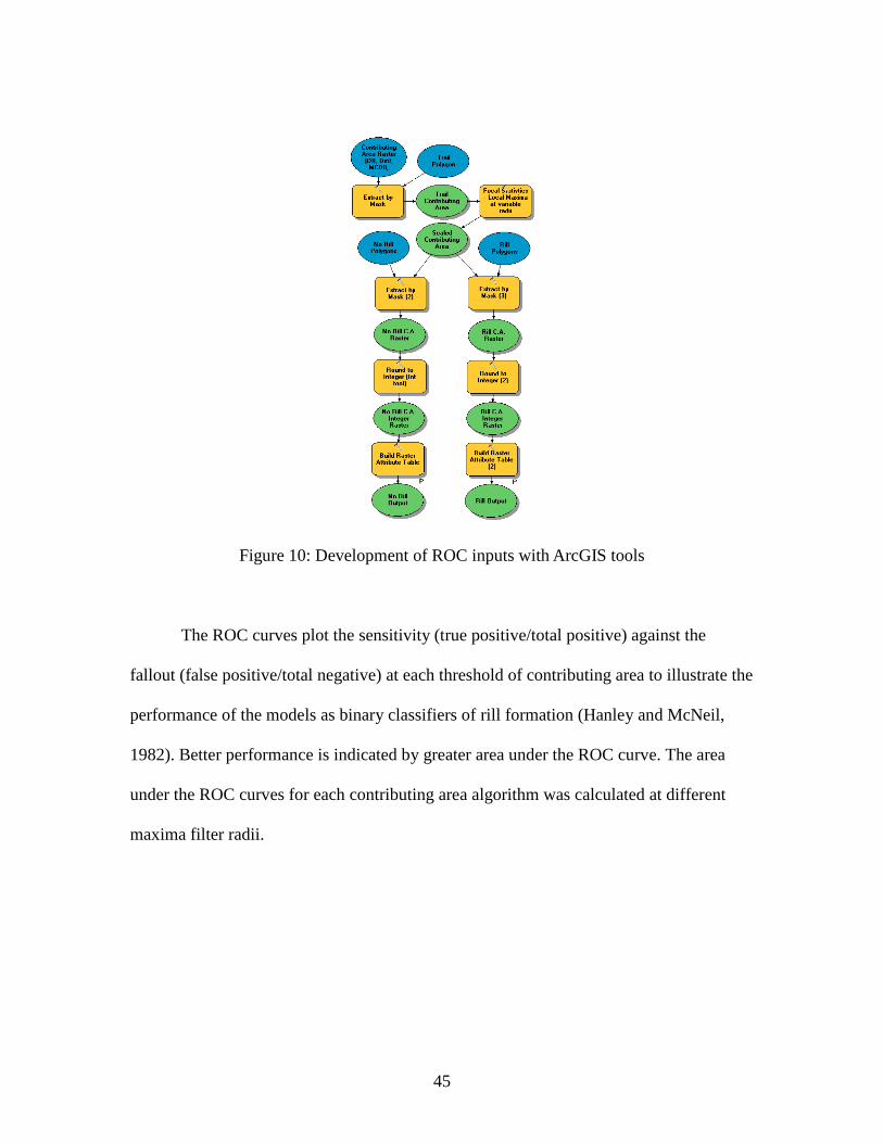
Figure 10: Development of ROC inputs with ArcGIS tools

The ROC curves plot the sensitivity (true positive/total positive) against the

fallout (false positive/total negative) at each threshold of contributing area to illustrate the

performance of the models as binary classifiers of rill formation (Hanley and McNeil,

1982). Better performance is indicated by greater area under the ROC curve. The area

under the ROC curves for each contributing area algorithm was calculated at different

maxima filter radii.

46

CHAPTER FOUR

RESULTS

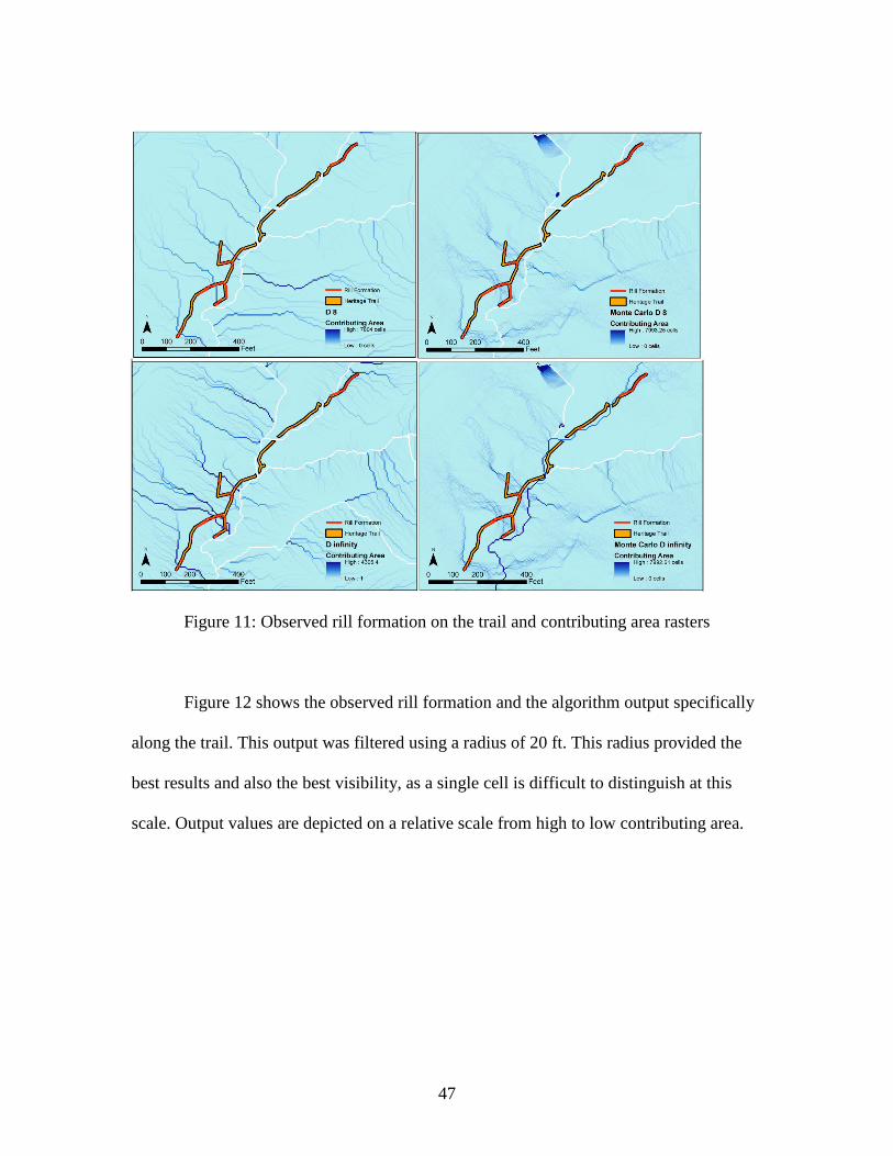
Figure 11 below shows the output of the contributing area algorithms including

the slopes above the trail. White lines represent the stream channels that were removed

from the analysis. The Monte Carlo D-infinity algorithm still includes one of the streams:

the random variability of the Monte Carlo technique combined with the flexibility of the

D-infinity algorithm made extraction of the stream network particularly difficult. To

avoid contributing area values in the stream channel from affecting the performance of

the algorithm in estimating rill formation risk along the trail, areas of the trail

corresponding to bridges were removed.

Another notable characteristic of the figure below is the flow in the South East

quadrant. The basic D-infinity algorithm routed flow very differently from the other

algorithms. In this area, flow follows alongside a road and is routed underneath the road

through culverts (see figure 4 above for the location of culverts). The other algorithms

provide general agreement on the flow path. It is unclear why the basic D-infinity

algorithm differs in this area, but it can be considered an error possibly stemming from

the necessary limitations that any algorithm faces in representing reality as a set of raster

cells.

Note especially the agreement between the two Monte Carlo outputs. It appears

the Monte Carlo technique yields convergent results between the D8 and D-infinity

algorithms.

47

Figure 11: Observed rill formation on the trail and contributing area rasters

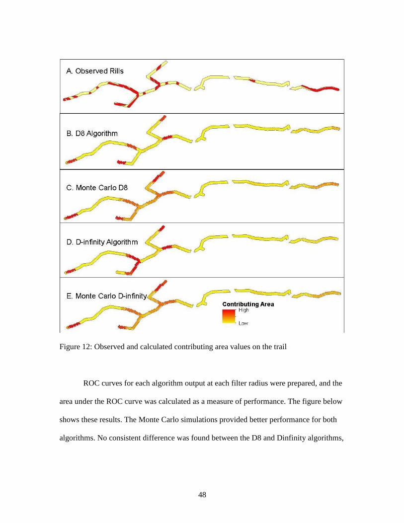
Figure 12 shows the observed rill formation and the algorithm output specifically

along the trail. This output was filtered using a radius of 20 ft. This radius provided the

best results and also the best visibility, as a single cell is difficult to distinguish at this

scale. Output values are depicted on a relative scale from high to low contributing area.

48

Figure 12: Observed and calculated contributing area values on the trail

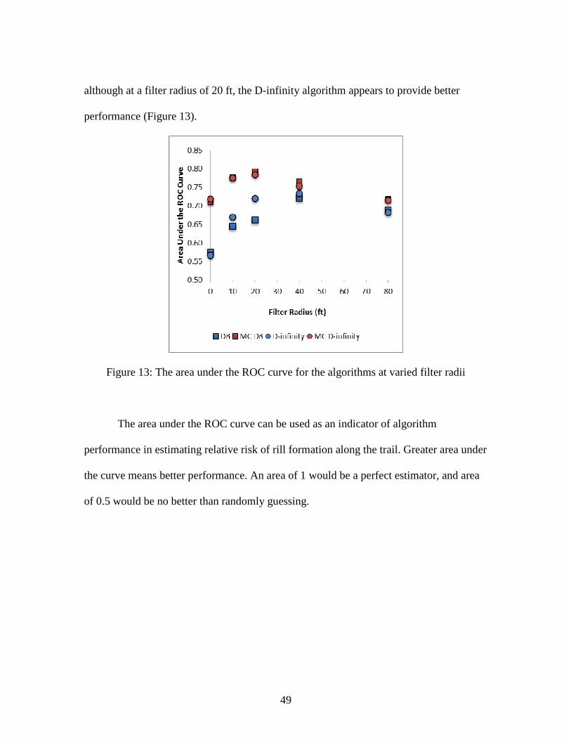
ROC curves for each algorithm output at each filter radius were prepared, and the

area under the ROC curve was calculated as a measure of performance. The figure below

shows these results. The Monte Carlo simulations provided better performance for both

algorithms. No consistent difference was found between the D8 and Dinfinity algorithms,

49

although at a filter radius of 20 ft, the D-infinity algorithm appears to provide better

performance (Figure 13).

Figure 13: The area under the ROC curve for the algorithms at varied filter radii

The area under the ROC curve can be used as an indicator of algorithm

performance in estimating relative risk of rill formation along the trail. Greater area under

the curve means better performance. An area of 1 would be a perfect estimator, and area

of 0.5 would be no better than randomly guessing.

50

CHAPTER FIVE

DISCUSSION

The D-infinity algorithm was expected to perform better than the D8 algorithm,

however, the difference was minimal and inconsistent. The D-infinity algorithm can

represent divergent flow patterns, while the D8 algorithm cannot. Divergent flow patterns

might be characteristic of sheet flow in the hill slopes and ponding in flat areas.

Concentrated surface flows which formed the rills observed along the trail were

apparently represented equivalently by the two algorithms.

The Monte Carlo technique implemented in the study did give a significant boost

to the performance of both algorithms. It appears that fine-scale error is a factor that

influences contributing area estimations at this scale in this landscape. Although the

Monte Carlo approach may be more robust, when considering additional factors such as

implementation and processing time, simply using the D8 or D-infinity algorithms may

be more suitable for practical applications. The Monte Carlo technique performed best at

a filter radius of 20 feet.

The basic D8 and D-infinity algorithms performed comparably to the Monte Carlo

techniques at a radius of 40 feet. Therefore, if very precise estimation is not needed, then

the basic D8 or D-infinity algorithms may be suitable. Identification of at risk areas at

scales of 20-40 feet may be close enough for designers and on-the-ground decision

makers to use the information.

51

If these results can be generalized to other landscapes and other forms of storm

water damage, then it is possible to create detailed and accurate models of storm water

runoff using LiDAR elevation data in conjunction with other high resolution datasets.

Location and sizing of various best management and low impact development practices

can be facilitated by methods such as described in this work. Currently, an addition to the

Natural Heritage Garden Trail is under construction, and the D-infinity algorithm has

been used to design diversion channels to prevent storm water damage in the future.

There are a number of directions in which this work may be carried further.

Estimation of surface characteristics relevant to runoff volume and velocity at a

resolution similar to a LiDAR DEM would enable very detailed analysis of runoff and

related processes such as erosion, transport, and deposition. The development of high

resolution elevation data motivates similar refinements in related spatial data. A

comparison of the ROC curves using different scales of resolution of the rill observations

could be informative. Just as the algorithm results were adjusted by expanding filters for

the highest estimates, the rill observations could be buffered at various widths. Such an

analysis could provide further insight on the appropriate scale at which to apply

algorithm results in practice. Another way of considering scale would be to use DEMs of

various cell sizes. Interpolation could be used to reduce the cell size, and averaging or

alternate data sources could be used with increased cell sizes.

The results of this study can be summarized by the assertion that LiDAR DEMs

can be useful in the design of infrastructure that affects or is affected by storm water

runoff. More specifically, this study has found that Monte Carlo techniques can

52

significantly increase the quality of contributing area datasets derived from a LiDAR

DEM.

53

BIBLIOGRAPHY

Baker, Matthew E., Donald E. Weller, and Thomas E. Jordan. 2006. "Comparison of Automated Watershed Delineations." Photogrammetric Engineering & Remote Sensing 72 (2): 159-168.

Barber, Christopher P. and Ashton Shortridge. 2005. "Lidar Elevation Data for Surface Hydrologic Modeling: Resolution and Representation Issues." Cartography and Geographic Information Science 32 (4): 401-410.

Barbosa, AE, JN Fernandes, and LM David. 2012. "Key Issues for Sustainable Urban Stormwater Management." Water Research 46 (20): 6787-6798.

Baumann, Jim. 2014. "GIS Insights Improve School Management." ArcUser, Summer.

Blair, A., D. Sanger, D. White, AF Holland, L. Vandiver, C. Bowker, and S. White. 2014. "Quantifying and Simulating Stormwater Runoff in Watersheds." Hydrological Processes 28 (3): 559-569.

Burns, Matthew J., Tim D. Fletcher, Christopher J. Walsh, Anthony R. Ladson, and Belinda E. Hatt. 2012. "Hydrologic Shortcomings of Conventional Urban Stormwater Management and Opportunities for Reform." Landscape and Urban Planning 105 (3): 230-240.

Calabria, Jon, William English, and Calvin Sawyer. 2006. Riparian Corridor Master Plan. Clemson University: Campus Planning Services.

Christian, Jason, Leonardo Duenas‐Osorio, Aarin Teague, Zheng Fang, and Philip Bedient. 2013. "Uncertainty in Floodplain Delineation: Expression of Flood Hazard and Risk in a Gulf Coast Watershed." Hydrological Processes 27 (19): 2774-2784.

Dhun, Kimberly. 2011.Application of LiDAR DEMs to the Modelling of Surface Drainage Patterns in Human Modified Landscapes.

ESRI. ArcGIS Resample Tool. 10.1st ed. Redlands, CA:.

Fairfield, John and Pierre Leymarie. 1991. "Drainage Networks from Grid Digital Elevation Models." Water Resources Research 27 (5): 709-717.

Fisher, Peter F. and Nicholas J. Tate. 2006. "Causes and Consequences of Error in Digital Elevation Models." Progress in Physical Geography 30 (4): 467-489.

Fletcher, TD, Herve Andrieu, and Perrine Hamel. 2013. "Understanding, Management and Modelling of Urban Hydrology and its Consequences for Receiving Waters: A State of the Art." Advances in Water Resources 51: 261-279.

54

Fletcher, Tim D., Geoff Vietz, and Christopher J. Walsh. 2014. "Protection of Stream Ecosystems from Urban Stormwater Runoff the Multiple Benefits of an Ecohydrological Approach." Progress in Physical Geography: 0309133314537671.

Florinsky, Igor V. 1998. "Combined Analysis of Digital Terrain Models and Remotely Sensed Data in Landscape Investigations." Progress in Physical Geography 22 (1): 33-60.

———. 2002. "Errors of Signal Processing in Digital Terrain Modelling." International Journal of Geographical Information Science 16 (5): 475-501.

Garbrecht, Jurgen and Lawrence W. Martz. 1999. An Overview of TOPAZ: An Automated Digital Landscape Analysis Tool for Topographic Evaluation, Drainage Identification, Watershed Segmentation, and Subcatchment Parameterization. El Reno, Oklahoma: Grazinglands Research Laboratory, USDA, Agricultural Research Service.

Gatziolis, Demetrios and Jeremy S. Fried. 2004. "Adding Gaussian Noise to Inaccurate Digital Elevation Models Improves Spatial Fidelity of Derived Drainage Networks." Water Resources Research 40 (2).

Gonzalez, Alvaro, Marouane Temimi, and Reza Khanbilvardi. 2014. "Adjustment to the Curve Number (NRCS–CN) to Account for the Vegetation Effect on the Hydrological Processes." Hydrological Sciences Journal (just-accepted).

Goulden, T., C. Hopkinson, R. Jamieson, and S. Sterling. 2014. "Sensitivity of Watershed Attributes to Spatial Resolution and Interpolation Method of LiDAR DEMs in Three Distinct Landscapes." Water Resources Research 50 (3): 1908-1927.

Grayson, Rodger and Günter Blöschl. 2001. Spatial Patterns in Catchment Hydrology: Observations and Modelling CUP Archive.

Grimaldi, Salvatore, Andrea Petroselli, Gustavo Alonso, and Fernando Nardi. 2010. "Flow Time Estimation with Spatially Variable Hillslope Velocity in Ungauged Basins." Advances in Water Resources 33 (10): 1216-1223.

Gyasi‐Agyei, Yeboah, Garry Willgoose, and Francois P. De Troch. 1995. "Effects of Vertical Resolution and Map Scale of Digital Elevation Models on Geomorphological Parameters used in Hydrology." Hydrological Processes 9 (3‐4): 363-382.

Hancock, GR. 2005. "The use of Digital Elevation Models in the Identification and Characterization of Catchments Over Different Grid Scales." Hydrological Processes 19 (9): 1727-1749.

55

Hellweger, Ferdi. "AGREE - DEM Surface Reconditioning System."2014, http://www.ce.utexas.edu/prof/maidment/gishydro/ferdi/research/agree/agree.html.

Heuvelink, Gerard BM. 1998. "Uncertainty Analysis in Environmental Modelling Under a Change of Spatial Scale." Nutrient Cycling in Agroecosystems 50 (1-3): 255-264.

Hopkinson, Chris, Laura E. Chasmer, Gabor Sass, Irena F. Creed, Michael Sitar, William Kalbfleisch, and Paul Treitz. 2005. "Vegetation Class Dependent Errors in Lidar Ground Elevation and Canopy Height Estimates in a Boreal Wetland Environment." Canadian Journal of Remote Sensing 31 (2): 191-206.

Huang, Mingbin, Jacques Gallichand, Zhanli Wang, and Monique Goulet. 2006. "A Modification to the Soil Conservation Service Curve Number Method for Steep Slopes in the Loess Plateau of China." Hydrological Processes 20 (3): 579-589.

ICCA. 2010. International Certified Crop Advisor Performance Objectives: American Society of Agronomy.

James, L. Allan, Darrell Glen Watson, and William F. Hansen. 2007. "Using LiDAR Data to Map Gullies and Headwater Streams Under Forest Canopy: South Carolina, USA." Catena 71 (1): 132-144.

Jenson, SK and JO Domingue. 1988. "Extracting Topographic Structure from Digital Elevation Data for Geographic Information System Analysis." Photogrammetric Engineering and Remote Sensing 54 (11): 1593-1600.

Laflen, John M., WJ Elliot, DC Flanagan, CR Meyer, and MA Nearing. 1997. "WEPP-Predicting Water Erosion using a Process-Based Model." Journal of Soil and Water Conservation 52 (2): 96-102.

Lemmens, MJPM. 1999. "Quality Description Problems of Blindly Sampled DEMs.".

Li, Ruopu, Zhenghong Tang, Xu Li, and Jessie Winter. 2013. "Drainage Structure Datasets and Effects on LiDAR-Derived Surface Flow Modeling." ISPRS International Journal of Geo-Information 2 (4): 1136-1152.

Liang, Chaojun and D. Scott MaCkay. 2000. "A General Model of Watershed Extraction and Representation using Globally Optimal Flow Paths and Up-Slope Contributing Areas." International Journal of Geographical Information Science 14 (4): 337-358.

Lindsay, John B. 2006. "Sensitivity of Channel Mapping Techniques to Uncertainty in Digital Elevation Data." International Journal of Geographical Information Science 20 (6): 669-692.

56

Lindsay, John B. and Irena F. Creed. 2006. "Distinguishing Actual and Artefact Depressions in Digital Elevation Data." Computers & Geosciences 32 (8): 1192-1204.

Lindsay, John B. and Martin G. Evans. 2008. "The Influence of Elevation Error on the Morphometrics of Channel Networks Extracted from DEMs and the Implications for Hydrological Modelling." Hydrological Processes 22 (11): 1588-1603.

Liu, Yuqiong and Hoshin V. Gupta. 2007. "Uncertainty in Hydrologic Modeling: Toward an Integrated Data Assimilation Framework." Water Resources Research 43 (7).

Maidment, D. 2002. Arc Hydro: GIS for Water Resources, edited by David R. Maidment. Redlands, CA: ESRI Press.

Mantelli, Luiz Rogério, Jomar Magalhães Barbosa, and Marisa Dantas Bitencourt. 2011. "Assessing Ecological Risk through Automated Drainage Extraction and Watershed Delineation." Ecological Informatics 6 (5): 325-331.

Martz, Lawrence W. and Jurgen Garbrecht. 1999. "An Outlet Breaching Algorithm for the Treatment of Closed Depressions in a Raster DEM." Computers & Geosciences 25 (7): 835-844.

———. 1998. "The Treatment of Flat Areas and Depressions in Automated Drainage Analysis of Raster Digital Elevation Models." Hydrological Processes 12 (6): 843-855.

McMillan, Patrick. "Natural Heritage Garden Trail."2014, http://www.clemson.edu/public/scbg/natural_heritage/index.html.

Meadows, Michael. 2014. "Adjusting NRCS Curve Number for Rainfall Durations Less than 24 Hours." Columbia, SC, .

Moore, Ian Donald, RB Grayson, and AR Ladson. 1991. "Digital Terrain Modelling: A Review of Hydrological, Geomorphological, and Biological Applications." Hydrological Processes 5 (1): 3-30.

Murphy, Paul NC, Jae Ogilvie, Fan‐Rui Meng, and Paul Arp. 2008. "Stream Network Modelling using Lidar and Photogrammetric Digital Elevation Models: A Comparison and Field Verification." Hydrological Processes 22 (12): 1747-1754.

NOAA. "LIDAR—Light Detection and Ranging—is a Remote Sensing Method used to Examine the Surface of the Earth. ."2014, http://oceanservice.noaa.gov/facts/lidar.html.

57

O'Callaghan, John F. and David M. Mark. 1984. "The Extraction of Drainage Networks from Digital Elevation Data." Computer Vision, Graphics, and Image Processing 28 (3): 323-344.

Oksanen, J. and T. Sarjakoski. 2005. "Error Propagation Analysis of DEM‐based Drainage Basin Delineation." International Journal of Remote Sensing 26 (14): 3085-3102.

Oksanen, Juha and Tapani Sarjakoski. 2006. "Uncovering the Statistical and Spatial Characteristics of Fine Toposcale DEM Error." International Journal of Geographical Information Science 20 (4): 345-369.

Petroselli, Andrea. 2012. "LIDAR Data and Hydrological Applications at the Basin Scale." GIScience & Remote Sensing 49 (1): 139-162.

Pourali, SH, C. Arrowsmith, D. Mitchell, and AA Matkan. 2014. "Modelling an Overland Water Flow Path in an Urban Catchment using GIS." Geoinformatica: An International Journal 4 (1).

Remmel, Tarmo K., Kenton W. Todd, and James Buttle. 2008. "A Comparison of Existing Surficial Hydrological Data Layers in a Low-Relief Forested Ontario Landscape with those Derived from a LiDAR DEM." The Forestry Chronicle 84 (6): 850-865.

Renschler, Chris S. 2003. "Designing Geo‐spatial Interfaces to Scale Process Models: The GeoWEPP Approach." Hydrological Processes 17 (5): 1005-1017.

Saghafian, Bahram, Amin Reza Meghdadi, and Somayeh Sima. 2014. "Application of the WEPP Model to Determine Sources of Run‐off and Sediment in a Forested Watershed." Hydrological Processes.

Saunders, William. 1999. "Preparation of DEMs for use in Environmental Modeling Analysis." San Diego, California, .

SCDHEC. 2005. Storm Water Management BMP Handbook: South Carolina Department of Health and Environmental Control.

SCDNR. "LiDAR Data Status by County.", accessed 11/6/2014, , http://www.dnr.sc.gov/GIS/lidarstatus.html.

Schwanghart, Wolfgang and Tobias Heckmann. 2012. "Fuzzy Delineation of Drainage Basins through Probabilistic Interpretation of Diverging Flow Algorithms." Environmental Modelling & Software 33: 106-113.

58

Tarboton, David G. 1997. "A New Method for the Determination of Flow Directions and Upslope Areas in Grid Digital Elevation Models." Water Resources Research 33 (2): 309-319.

Tarboton, David G. and Ibrahim N. Mohammed. 2013. TauDEM 5.1 QUICK START GUIDE TO USING THE TAUDEM ARCGIS TOOLBOX Utah State University.

Tarboton, David G. and Daniel P. Ames. 2001. "Advances in the Mapping of Flow Networks from Digital Elevation Data."Am. Soc Civil Engrs USA, .

Thapa, Khagendra and John Bossler. 1992. "Accuracy of Spatial Data used in Geographic Information Systems." Photogrammetric Engineering and Remote Sensing 58 (6): 835-841.

Threatt, Jimmy. 2014. Clemson LiDAR Metadata.

Torri, D., M. Sfalanga, and M. Del Sette. 1987. "Splash Detachment: Runoff Depth and Soil Cohesion." Catena 14 (1): 149-155.

Tribe, Andrea. 1992. "Automated Recognition of Valley Lines and Drainage Networks from Grid Digital Elevation Models: A Review and a New Method." Journal of Hydrology 139 (1): 263-293.

Ukkonen, Tomas, Tapani Sarjakoski, and Juha Oksanen. 2007. "Distributed Computation of Drainage Basin Delineations from Uncertain Digital Elevation Models."ACM, .

USGS. "National Elevation Dataset.", last modified 4/15/2014, accessed 11/5/2014, , ned.usgs.gov.

———. "National Hydrography Dataset.", http://nhd.usgs.gov/.

———. "Shuttle Radar Topography Mission.", last modified 9/30/2010, accessed 11/5/2014, , srtm.usgs.gov.

Vesakoski, Jenni-Mari, Petteri Alho, Juha Hyyppä, Markus Holopainen, Claude Flener, and Hannu Hyyppä. 2014. "Nationwide Digital Terrain Models for Topographic Depression Modelling in Detection of Flood Detention Areas." Water 6 (2): 271-300.

Walsh, Christopher J., Tim D. Fletcher, and Matthew J. Burns. 2012. "Urban Stormwater Runoff: A New Class of Environmental Flow Problem." PloS One 7 (9): e45814.

Wang, L. and H. Liu. 2006. "An Efficient Method for Identifying and Filling Surface Depressions in Digital Elevation Models for Hydrologic Analysis and Modelling." International Journal of Geographical Information Science 20 (2): 193-213.

59

Wise, STEVE M. 1998. "The Effect of GIS Interpolation Errors on the use of Digital Elevation Models in Geomorphology." Landform Monitoring, Modelling and Analysis 99: 139-164.

Yao, C., T. Lei, WJ Elliot, DK McCool, J. Zhao, and S. Chen. 2008. "Critical Conditions for Rill Initiation." Transactions of the ASAE (American Society of Agricultural Engineers) 51 (1): 107.

Zandbergen, Paul A. 2010. "Accuracy Considerations in the Analysis of Depressions in Medium-Resolution LIDAR DEMs." GIScience & Remote Sensing 47 (2): 187-207.

———. 2011. "Error Propagation Modeling for Terrain Analysis using Dynamic Simulation Tools in ArcGIS Modelbuilder." Geomorphometry: 57-60.