Graduate Theses, Dissertations, and Problem Reports

2009

Stock returns, risk factor loadings, and model predictions: A test Stock returns, risk factor loadings, and model predictions: A test

of the CAPM and the Fama -French 3 -factor model of the CAPM and the Fama -French 3 -factor model

Daniel Suh West Virginia University

Follow this and additional works at: https://researchrepository.wvu.edu/etd

Recommended Citation Recommended Citation Suh, Daniel, "Stock returns, risk factor loadings, and model predictions: A test of the CAPM and the Fama -French 3 -factor model" (2009). Graduate Theses, Dissertations, and Problem Reports. 2944. https://researchrepository.wvu.edu/etd/2944

This Dissertation is protected by copyright and/or related rights. It has been brought to you by the The Research Repository @ WVU with permission from the rights-holder(s). You are free to use this Dissertation in any way that is permitted by the copyright and related rights legislation that applies to your use. For other uses you must obtain permission from the rights-holder(s) directly, unless additional rights are indicated by a Creative Commons license in the record and/ or on the work itself. This Dissertation has been accepted for inclusion in WVU Graduate Theses, Dissertations, and Problem Reports collection by an authorized administrator of The Research Repository @ WVU. For more information, please contact researchrepository@mail.wvu.edu.

Stock Returns, Risk Factor Loadings, and Model Predictions: A Test of the CAPM and the Fama-French 3-factor Model

Daniel Suh

Dissertation submitted to the College of Business and Economics

at West Virginia University in partial fulfillment of the requirements

for the degree of

Doctor of Philosophy in

Economics

Ashok B. Abbott, Ph.D., Chair Ronald Balvers, Ph.D.

Victor Chow, Ph.D. Strafford Douglas, Ph.D. Alexander Kurov, Ph.D.

Department of Economics

Morgantown, West Virginia

2009

Key words: Asset Pricing Model, Cost of Equity Capital, The CAPM, The Fama-French model and portfolios, market portfolio, Risk Premium, Risk Factor Loadings

Abstract

Stock Returns, Risk Factor Loadings, and Model Predictions:

A Test on the CAPM and the Fama-French 3-factor Model

Daniel Suh

This paper presents the results of time-series tests of the Capital Asset Pricing Model (CAPM) and the Fama-French 3-factor (FF3) model in the estimation of equity capital from a perspective of corporate investment decision-making. The CAPM, the single-factor or market-factor model, has been taught and tested as the primary asset pricing model in academia and used in business for the estimation of the cost of equity capital. On the other hand, the FF3 model has been widely used in academic research for testing asset pricing models mostly on portfolios. This paper addresses Fama-French (1992, “The Cross-section of Expected Stock Returns,” Journal of Finance) who find that the CAPM beta has little explanatory power in cross-sectional tests of the Fama-French portfolios sorted on market capitalization and book-to-market ratios. The main tests of this paper are (1) the equivalence of the predicted stock risk premia of the CAPM and the FF3 model, or how significantly the two model-predicted stock risk premia are correlated with the realized returns and (2) the inter-temporal and cross-sectional shift of the market beta regimes. This paper tests the CAPM and the FF3 model on daily returns of a wide range of individual stocks and Fama-French portfolios. All statistical tests are conducted on an individual stock and portfolio level.

The regression test results of the factor loadings underline the similarities and dissimilarities between the CAPM and the FF3 model applied on individual stocks and the FF portfolios. The most consistent finding throughout the tests in this paper is that the market index is the most significant risk factor loading among three risk factors (the market index, SMB, and HML) throughout the test period and across individual stocks and the Fama-French portfolios. For individual stocks, the market index is the most significant factor loading alone or in combination with SMB and HML. The statistical explanatory power of the CAPM beta of individual stocks has inter-temporally increased, particularly for micro-cap stocks. The test of individual stocks does not reject the null hypothesis that the predicted risk permia of both models are equivalent. The overall time-series test results on individual stocks and portfolios contrast with Fama-French (1992). On the other hand, the FF3-predicted risk premia for the FF25 portfolios largely outperform the CAPM predictions. The most intriguing finding on the risk factor loadings is that the market index rarely is significant by itself for the Fama-French 25 (FF25) portfolios within the FF3 model. For the FF25 portfolios within the FF3 model, the market index loadings mostly become significant in combination with SMB, HML, or both, but not alone. SMB and HML are insignificant alone or in combination with each other for the FF25 portfolios. However, the two factors become as nearly significant as the market index in combination with the market index.

The turnabout is a stark contrast with the evidence that the market beta is more significant by itself for the majority of individual stocks in the FF3 model than in combination with two other factors. The turnabout is intriguing in that the market index loadings are statistically significant for every regression for all FF25 portfolios in the FF3 model in combination with SMB, HML, or both. It’s even more intriguing that the CAPM betas also are statistically significant for every regression for all FF25 portfolios; the CAPM beta is not always significant for all individual regressions, however. It’s puzzling that SMB and HML are not significant by itself or in combination with each other for any FF portfolios, but become as nearly significant as the market index when combined with the market index for the FF25 portfolios. For the FF25 portfolios, no factor is significant by itself, but factors become highly significant in combination with the market index. A risk factor becomes significant mostly in combination with other factor for the FF25 portfolios within the FF3 model. The CAPM and the FF3 model in general are statistically equivalent in explaining individual stock returns. However, the two models are diametrically dissimilar in explaining the FF25 portfolios. The CAPM best explains large/growth (LG) portfolio returns, but is poor in explaining small/value (SV) portfolios. The high explanatory power of the CAPM for all LG portfolios is consistent, and so is the poor explanatory power for SV portfolios. The distinctive explanatory power of the CAPM between LG portfolios and SV portfolios is clear and unambiguous, and is consistent with the CAPM or the market model structure. On the other hand, the FF3 model best explains small/value (SV) portfolios, a direct opposite of the CAPM. The FF3 model is most poor in explaining large/value (LV), not LG portfolios. In the FF3 model, the “value” portfolios are at both extremes in explanatory power. Unlike the CAPM, most growth portfolios are located in the middle of the rank-order in the explanatory power of the FF3 model. The virtual diametrical dissimilarities in explanatory power between the CAPM and the FF3 model for the FF25 portfolio and the statistical equivalence of the two models for individual stocks underline the unique return factor structures of the FF portfolios and the two risk factors (SMB and HML). The superiority of the CAPM in explaining large-cap growth stocks and the inferiority of the FF3 model in explaining large-value growth may undermine the application value of the FF3 model for the estimation of the cost of equity capital. The results of test of out-of-sample forecast using 5-year rolling regressions on monthly stock returns confirm all major findings of the test using daily data and conditioning information. For individual stocks, the mean squared errors of the out-of-sample forecast of the CAPM and the FF3 model are statistically equal, but the MSEs for the FF25 portfolios are not. The test also confirms that the market index is the most consistently significant risk factor.

The cross-sectional factor loadings and statistics of the CAPM and the FF3 model for the FF25 portfolios are distinctly dissimilar. The factor structure of the FF25 portfolios appears to induce statistically significant factor loadings of SMB and HML, which are constructed on the FF25 portfolio return structure the two factors are supposed to explain. Nevertheless, the economic meaning and investment applicability of the two factor loadings are unclear.

I conduct a focused test for inter-temporal and cross-sectional regime-shift of the market beta. The test is conducted on the individual firms of the electric power industry, which has been going through a restructuring and deregulation process since the 1990s. This paper focuses on the identification of the economic sources of the regime shift, as the market and industry environment changes and a firm’s investment model and financing strategy evolve. To gain conditioning information, I examine the industry restructuring process at the market, government policy, and corporate investment and financing strategy.

The test rejects the hypothesis of inter-temporal and cross-sectional constancy of beta regimes. The return volatilities of the firms which adopted competitive merchant power business dramatically increased during the restructuring period, and cross-sectionally moved their beta estimates higher and away from those firms which largely remained in the traditional utility business. The higher betas of competitive business than traditional utility business appear to have come in large part from the increased exposures to common systematic factors.

v

Dedication

I owe my greatest debt to my parents and my wife, Mary. My parents had eagerly waited for me to complete my doctoral program and become a professor. During my dissertation research, however, both of my parents left this world after prolonged illness and suffering. On completion of this dissertation, I feel heart-broken rather than joyful because I cannot share it with my parents. I dedicate this dissertation to my parents with crying tears. My wife, Mary, has whole-heartedly supported my doctoral training. She says that it is her joy to see me enjoy study and research, and has persistently encouraged me to be devoted to quality research regardless of monetary benefit. The real doctoral degree belongs to my wife; I merely get a certificate on her behalf. I also owe a debt to my brother, Euiho, who is more joyful, excited, and proud than I am. Euiho thinks that his brother will become one of the best scholars in the world. I also dedicate this dissertation to my grandmother and my aunt, who raised me with love and sacrifice in the war-devastated, impoverished conditions. Without my parents and grandmother, my aunt is my mother and father.

vi

Acknowledgment

I owe a great debt to my dissertation committee members. Dr. Ashok Abbott, the chair of the committee, always has been positive, optimistic, and encouraging. Every discussion with Dr. Abbott gave me a new idea and led me in a new direction. He directed me to include a test of the Fama-French model as well as the CAPM in an initial version of this dissertation. Discussions with Dr. Ronald Balvers always have been deep and serious. He emphasizes high quality of scholarly research and the fundamentals of ideas. This dissertation is an outgrowth of my paper for his asset pricing course and the subsequent drafts under his supervision. I truly appreciate his prompt feedback and numerous discussions with me. Dr. Strafford Douglas put me under his wings as my mentor, immediately when I began my doctoral study. I had had weekly conversations and discussions with him on the electric power industry and academic research. Chapter 3 of this dissertation is an outgrowth of my numerous discussions with him. Dr. Victor Chow always has been straight, open, and realistic. He helped me better balanced between academic rigors and the practical applications of theory. Dr. Alexander Kurov has freely shared research ideas and resources with me. Upon review of my very first crude draft, he said straight that it was not a test of the CAPM although the initial title had the name.

vii

Stock Returns, Risk Factor Loadings, and Model Predictions: A Test on the CAPM and the Fama-French 3-factor Model

Chapter 1: Systematic Risk and Asset Pricing Models

Chapter Abstract

1. Asset Pricing Models A. The Capital Asset Pricing Model (CAPM) ............................................................................ 2 B. Alternative Asset Pricing Models ........................................................................................ 6 C. The Fama-French 3-factor (FF3) Model ............................................................................. 9

2. Research Objectives and Design A. Research Objectives and Hypotheses ............................................................................... 18 B. Test Framework ................................................................................................................ 20 C. Research Approach ........................................................................................................... 23 D. Data ................................................................................................................................... 27 E. Limitations ........................................................................................................................ 29

3. Concluding Summary ..................................................................................................................... 31

References ............................................................................................................................................ 33

Chapter 2: Factor Loadings and Model Predictions

Chapter Abstract

1. Risk Factor Loadings A. Model Specification Tests.43

a. Significance of Risk Factor Loadings ........................................................................... 43 b. SMB and HML in the Fama-French Portfolios ............................................................ 45 c. Alpha Estimates.46 d. Regressions of No Significant Loadings and Alpha ..................................................... 48 e. Time-invariance of Factor Loadings of Fama-French Portfolios ................................. 49

B. Regression Diagnostics ..................................................................................................... 50

2. Model-predicted Risk Premium .................................................................................................... 52 A. Large-cap and Dow Jones Index Stocks ............................................................................ 53 B. Micro-cap and Electric power stocks ............................................................................... 54 C. Fama-French Portfolios .................................................................................................... 55

3. Out-of-Sample Forecasts .............................................................................................................. 56 4. Concluding Summary .................................................................................................................... 58

References ............................................................................................................................................ 61

viii

Appendix ............................................................................................................................................... 62 Exhibits ................................................................................................................................................. 94

Chapter 3: Industry Restructuring, Market Risk, and the Market Beta Regime

Chapter Abstracts

1. Industry Restructuring and Market Risk .................................................................................... .102 2. Research Design ........................................................................................................................... 103 3. Investment, Financing Strategy, and Systematic Risk .................................................................. 108 4. Hypothesis on Beta Regimes ....................................................................................................... 110 5. Factor Loadings and Model Predictions

A. Estimates of Risk Factor Loadings .................................................................................. 112 B. Model-predicted vs. Realized Returns ............................................................................ 114 C. Shifts of Market Beta Regimes ....................................................................................... 115

i. Inter-temporal shift .......................................................................................... 115 ii. Cross-sectional shift ........................................................................................... 116

D. Structural Breaks ............................................................................................................. 118 6. Concluding Summary .................................................................................................................. 118

Appendix on the Industry Restructuring ........................................................................................... 120 References ......................................................................................................................................... 129 Appendix ............................................................................................................................................ 131

ix

List of Tables

Chapter 2

Table 1-1 Test Sample Data .............................................................................................................. 62 Table 1-1-1 Model Specifications – Annual estimations ..................................................................... 63 Table 1-1-2 Model Specifications – Quarterly estimations ................................................................. 65 Table 1-2-1 Test for Omitted Variables (F-tests) ................................................................................. 67 Table 1-2-2 Residual test for Serial Correlations and Heteroskedasticiy ............................................ 69 Table 1-3 R2, Factor Loading Estimates, and Variability ................................................................... 77 Table 2-1 Model-estimated stock returns vs. the realized returns ................................................. 79 Table 2-2 Model-estimated stock returns vs. the realized returns ................................................. 81 Table 2-3-1 Model-estimated stock returns vs. the realized returns ................................................. 83 Table 2-3-2 Model-predictions of the FF25 Portfolio Returns ............................................................ 84 Table 2-4-1 F-tests for Equality of Mean Squared Errors (MSEs) ....................................................... .85 Table 2-4-2 Rolling Regression Specifications ...................................................................................... 86 Table 2-4-3 Mean Squared Errors of one-period-ahead forecasts: Dow Jones Index Stocks .............. 87 Table 2-4-4 Mean Squared Errors of one-period-ahead forecasts: Large-cap Stocks ........................ 88 Table 2-4-5 Mean Squared Errors of one-period-ahead forecasts: Micro-cap Stocks ........................ 89 Chapter 3 Table 1 Stock Price Changes during the Industry Crisis (2000Q4-2003Q1) ................................ 131 Table 2 Model Specification and Parameter Estimates .............................................................. 132 Table 3 Number of Significant Betas and Insignificant Alphas ................................................... 133 Table 4 Correlations between Model-predicted stock returns and Realized returns ................ 134 Table 5-1 Test for Time-varying Beta ............................................................................................. 135 Table 5-2 Test for Cross-sectional Equivalence of Two Business Groups ...................................... 136

x

List of Figures

Chapter 1 Figure 1 Percent of zero-return data ............................................................................................. 49 Figure 2 Stocks by Prime Exchange ................................................................................................ 49 Figure 3 Percent of Zero-Return Data (Micro-cap stocks) ............................................................. 50 Figure 4 Percent of Zero-Return Data by Stock Group .................................................................. 50

Chapter 2

Figure 1-1 Regression Diagnostics ..................................................................................................... 90 Exhibits to Tables 1-1-1 and1-1-2 .............................................................................................................. 94

Chapter 3 Figure A1-1 Stock Prices .................................................................................................................... 126 Figure A1-2 New Capacity Installations ............................................................................................. 126 Figure A1-3 Capacity Margin ............................................................................................................. 126 Figure A2 Investment and Financing .............................................................................................. 127 Figure A3 Liquidity and Solvency ................................................................................................... 128 Figure 1 Stock Price Changes ....................................................................................................... 137 Figures 2-1 Investing Activities ......................................................................................................... 139 Figures 2-2 Financing Activities ........................................................................................................ 140 Figure 2-3 Net Income and Operating Cash Flows .......................................................................... 142 Figure 3-1-1 Beta estimates ............................................................................................................... 143 Figure 3-1-2 Alpha estimates ............................................................................................................. 143 Figure 3-1-3 Adjusted R2 ..................................................................................................................... 144 Figure 3-1-4 SBC ................................................................................................................................. 144 Figure 4 Beta Coefficient Breakpoints ......................................................................................... 145 List of Firms ............................................................................................................................................... 146

1

Chapter 1

Systematic Risks and Model Predictions

Chapter 1 discusses asset pricing models and lays out research objectives, research approach, test framework, and test data construction. This chapter begins with a review of the theoretical development and empirical tests of asset pricing models with a focus on the Capital Asset Pricing Model (CAPM) and the Fama-French 3-factor (FF3) model. Decades of empirical tests of the theoretical asset pricing models have been mixed or inconclusive, and debate continues. Consumer utility function, a theoretically fundamental factor in asset pricing, is difficult to define and measure. The suggested systematic risk factors have not been robust in empirical test, or lack solid theoretical basis. Notwithstanding the return “abnormalities” not explained by the CAPM, the single-factor market-factor model has been taught and tested as the primary asset pricing model in academia and used in business to estimate the cost of equity capital. On the other hand, the FF3 model has been widely used in academic research for testing asset pricing models mostly on portfolios sorted on market capitalization and book-to-market capitalization ratio.

The objective of this paper is to conduct time-series tests of the Capital Asset Pricing Model (CAPM) and the Fama-French three-factor (FF3) model from a perspective of a corporate manager who uses the two models to estimate the cost of equity capital of the firm. This paper has two main research objectives: (1) Test the model predictability of the realized returns or how closely the model-predicted stock returns are correlated with the realized returns; this is the main test of this paper; and (2) Test for inter-temporal and cross-sectional regime-shift of market beta and identify the economic sources of regime-shift as the market and industry environments change and a firm’s investment model and financing strategy evolve. This paper uses conditioning information in research design, tests, and economic interpretations of the test results, and conduct investigations at disaggregated or firm levels. This paper conducts tests also on a variety of individual stocks and the Fama-French portfolios. This approach contrasts with most tests of asset pricing models including FF (1992, 1993, 1996) in the literature that are conducted exclusively on Fama-French portfolios, sorted on capitalization and book-to-market ratio.

2

1 Asset Pricing Models This section reviews the development of asset pricing models and the challenges in empirical

testing of the models, with a main focus on the Capital Asset Pricing Mode (CAPM) and the Fama-

French 3-factor (FF3) model. The former has been widely tested and taught in academia and applied in

business for the estimation of cost of capital and systematic risk measure. The latter is widely used in

academia for empirical test of asset pricing models. Most tests of asset pricing models in the literature are

conducted on Fama-French portfolios sorted on capitalization and book-to-market ratio. No other

alternative asset pricing models have been as widely taught and applied as the CAPM and as widely

tested in recent academic research as the FF3 model.

A. The Capital Asset Pricing Model (CAPM)

Asset pricing models provide estimates for the expected returns of an investment, a critical factor

in the determination of an asset or portfolio value. However, empirical test results of asset pricing models

have been disappointing. For example, the Capital Asset Pricing Model (CAPM) is “one of the two or

three major contributions of academic research to financial managers during the post-war era.”

(Jagannathan and Wang, 1996, p.4) However, Roll (1988) finds his test results of the CAPM “extremely

disappointing.” Roll find that with “all explanatory factors” included, less than 40% of the monthly

return volatility in the typical stock can be explained for a sample of the largest firms; explanatory power

with daily data is even less. 1

Fama and French (1992) find little explanatory power of CAPM beta even when the beta is used

as a single factor in a cross-sectional test on 25 portfolios sorted on market capitalization and book-to-

market ratio. Fama-French (1993, p.54) argues that the “common habit” of using the CAPM to evaluate

portfolio performance and to estimate the cost of capital should be broken. Fama-French (1996) put up a

sign, “The CAPM is wanted, dead or alive.” Fama and French (1997) test both the CAPM and the Fama-

French 3-factor (FF3) model, and find that the forecast performance of both models is “woefully

imprecise.”

2

1 At the same time, Roll (1988) finds some firms with “impressive explanatory power” and suggests an in-depth study of those firms “for insight.” 2 Forecastability of financial prices is one of the most enduring questions in finance and investment. (Campbell et al., 1997, p.27) Roll (1988) notes: “The maturity of science is often gauged by its success in predicting important phenomena… The immaturity of our science [finance] is illustrated by the conspicuous lack of predictive content about some of its most intensely interesting phenomena, particularly changes in asset prices.”

Fama and French (1997) note that imprecise estimates of risk loadings and factor risk

premium “plague industry CE [costs of equity] estimates from any asset pricing model.” (Italics added)

Hodrick and Zhang (2001) test a variety of empirical asset pricing models developed as potential

3

improvements on the CAPM and report that all of the models fail. 3

3 Hodrick and Zhang (2001) test the CAPM, the consumption CAPM, the conditional CAPM, Campbell’s (1996) log-linear model, Cochrane’s (1996) production-based model, and Fama-French’s three- and five-factor models.

Ferson and Harvey (1999, p.1325)

declared, “Empirical asset pricing is in a state of turmoil.”

Moreover, Roll (1977) critiques that CAPM test is about the mean-variance efficiency of the

market portfolio; therefore if the market portfolio fails to include all risky assets, a true test of the CAPM

is impossible. Meanwhile, empirical research has documented common stock return anomalies not

explained by the CAPM (e.g., Banz, 1981 for size or market capitalization effects) and largely rejects the

model (e.g., Reinganum, 1981; Fama and French, 1992). However, Cochrane (2005, p.126) observes that

none of the claimed “puzzles” and “anomalies” documents an exploitable arbitrage opportunity. While

recognizing the economically important anomalies or deviations of the CAPM, Campbell, et al. (1997,

p.212) notice little theoretical motivation for the firm characteristics in the literature that finds anomalies;

they argue that this opens up a possibility to overstate the evidence against the CAPM.

Alternative models have been proposed. Among the major asset pricing models are Merton’s

(1973) Inter-temporal CAPM, Ross’ (1976) Arbitrage Pricing Model, Breeden’s (1979) Consumption

CAPM, Fama-French’s (1992, 1993) 3-factor model, Jagannathan and Wang’s (1996) conditional CAPM,

and Cochrane’s (1996) Investment-based CAPM. Empirical multifactor models also have been tested as

alternatives to the CAPM. Chen et al. (1986) identify macro variables such as GDP, inflation, and

interest rate term structure as systematic risk factors. Fama and French (1992, 1993) identify market

capitalization (size) and book-to-market as systematic risk factors.

However, Fama (1991, p.1594) calls multifactor models “an empiricist’s dream,” because they

are “off-the-shelf theories” that can use “any set of factors that are correlated with returns.” Cochrane

(2005, pp.80, 124-126) observes that multifactor modeling can be “vacuous” because “a regression of

anything on anything” can be run; pricing factors should be robust across samples or different markets

and out of samples; since Merton (1973) and Ross (1976), the standard set of risk factors have changed

about every two years. Cochran (2005, p.151) further notes that the identities of fundamental risk factors

are still an unanswered question in finance; 30 or 40 years of thousands of papers have not moved the

debate an inch closer to resolution and a ready solution is not immediately in sight. Friend (1973)

“strongly” suspected that “50 years from now our successors will be engaged in more and more elaborate

curve fitting of aggregate time-series data which will explain the sample period even better than … now,

but are no more successful in predicting the consequences of policy action.”

4

The CAPM is a static and steady-state equilibrium model for one period with assumptions of

rational expectations, same investment opportunities, homogenous information on investment

opportunities, and same interpretation of investment return characteristics (e.g., expected returns, standard

deviation of return, and the correlations among asset returns) by all investors in frictionless and perfectly

competitive financial markets (i.e., infinitely divisible assets, no transaction costs, no taxes and

restrictions on short-selling, same borrowing and lending cost). 4

The CAPM is analogous to the theory of perfect competition in microeconomics, to the theory of

permanent income hypothesis in macroeconomics, to the theory of purchasing power parity (PPP) in

international economics, to the expectations theory on the term structure of interest rates in monetary

economics, and to the Miller-Modigliani Irrelevance theory in corporate finance. Each theory, highly

intuitive and deceptively simple, stands high as a benchmark or baseline model in its field.

(Fama and French, 2004, pp. 15, 16)

5 Similar to the

CAPM, these theories generally assume perfect information or rational expectation, frictionless markets,

and perfectly rational agents. However, key variables of these useful theoretical constructs such as

demand schedule and permanent income are difficult to measure; empirical tests with the realized data

have failed to fully confirm these theories, and controversies have continued.6

Among the most challenging issues in empirical tests of economic and finance theory based on

realized variables is the rational expectations assumption of economic and finance theories and models.

Merton (1980) recognizes this challenge in asset pricing as a main reason for the scarcity of research

estimating expected returns.

7

4 The appropriate length of the period for a single-period model is an important issue, particularly in the test of the CAPM. However, very little research has been done. (Elton and Gruber, 1997) Merton’s (1980, p.336) test takes a month as the “observation interval,” during which the market variance and riskless rate are assumed to be constant; as long as daily data is available. Merton’s argument for the monthly interval: a monthly interval is short enough so that the variation in the variation rate over the interval is substantially smaller than the variation in realized returns. Observation interval is a relevant issue in Section 3 of this chapter on the Research Design of this paper. 5 Box (1976) notes: “as the ability to devise simple but evocative models is the signature of the great scientist, so over-elaboration and over-parameterization is often the mark of mediocrity… Since all models are wrong, the scientist must be alert to what is importantly wrong. It is inappropriate to be concerned about mice when there are tigers abroad” 6 Kennedy (2003, p.81) notes: the traditional view that economic theory is accurate and econometrics provide good estimates have been replaced by a general acknowledgment that models are “false” and there is “no hope or pretense” to find “truth” through models. Kennedy quotes M.S. Feldstein: “(A) useful model is not one that is ‘true’ or ‘realistic’ … but parsimonious, plausible and informative.” Kennedy also quotes Henry Theil and D. Quah: “Models are to be used, but not to be believed;” models are “simply rough guides to understanding.”

Merton also points out a serious flaw in using historical averages based on

7 Let alone the measurement problem of investor expectations, the timing of formation of expectations is a challenge for researchers. For example, investor expectations of regulatory changes or industry restructuring policy take shape long before formal events or announcements. In the early 1990s, state regulatory bodies actively began proceedings to restructure the electric power industry, long before California became the first state to formal deregulation of its electric power market effective in April 1998. Two years before the formal deregulation, the legislature had enacted

5

rational expectations hypothesis, which ignores the effect of changes in the level of market risk. Hendry

(1980, p.396) refers to Keynes’ assertion that no economic theory is ever testable because problems in

economic “science” include omitted variables bias, models with unobservable variables such as

expectations, estimates based on badly measured data, spurious correlations from the use of proxy

variables and simultaneity, unknown functional forms, misspecification of dynamic reactions and lag

strengths, incorrect pre-filtering of data, etc.

The CAPM specifies a linear relationship between the expected excess return (risk premium) of

an asset and the expected excess market return (or market risk premium, MRP) in equilibrium. The

theoretical CAPM beta is forward-looking and the model is based on the investor’s rational expectations.

In the real world, however, the market portfolio is undefined. In addition, market portfolio in equilibrium

is unobservable and unknown; an economic equilibrium is a moving target. (Sharpe, 2007, p.9)

Furthermore, neither frictionless is the financial market, nor perfect and homogenous are the market

information and its interpretation of all investors; in addition, investors are not always rational. Fama and

French (2004) suggest that the CAPM has never been tested because of the mean-variance inefficiency of

the market portfolio proxies used in empirical tests. At the same time, they recognize that the same

criticism can be made on the tests of any economic model when a proxy is used.

Roll (1977) challenges the CAPM on the testability and the validity of the model because of the

unobservable true market portfolio, mean-variance inefficiency of market portfolio proxy, and

tautological relation between the linearity of the CAPM beta (with the returns) and mean-variance

efficiency of the market portfolio. Roll declared that a correct and unambiguous test of the CAPM had

not been made, nor is practically possible. Roll and Ross (1994) show that if the true market portfolio is

efficient, the cross-sectional relation between expected returns and beta can be very sensitive to small

deviations of market portfolio proxy from the true market portfolios. Kandel and Stambaugh (1995) also

show that when the market portfolio is inefficient, the OLS estimates of the CAPM have no relation with

the mean-variance location of the index.8

deregulation and allowed California power firms two-year transition into deregulation. Binder (1985) finds that it’s difficult to detect effects of deregulation and restructuring on stock prices because formal events or announcements rarely contain major new information. Binder finds no difference in information contents between monthly and daily data and attributes it to investors’ anticipation of formal events or announcement. Public firms would face similar challenges. 8 Roll (1978) shows that for every ranking of performance obtained with a mean-variance non-efficient index, another non-efficient index exists which reverses the ranking. Using Dow-Jone30 firm stock returns, Benninga (2008) demonstrates a “mysterious portfolio” index, similar to Kandel and Stambaugh (1995) who use 10-portfolio index.

Campbell et al. (1997, p. 216-217) note that use of market

portfolio proxy in empirical work could have “forced” the lack of a cross-sectional relation between mean

6

returns and beta.9 However, Campbell et al. (1997, p. 214, 215) note that Roll’s concern about the mean-

variance efficiency of the market portfolio is not an empirical problem.10

B. Alternative Asset Pricing Models

Roll (1994) recognizes that it’s

unclear whether an “inappropriate proxy” for the market portfolio is really the correct explanation for the

rejection of the CAPM.

Cochrane (2005, p.3, 41) calls the consumption-based asset pricing model a complete answer to

“all” asset pricing questions in principle, because asset prices should be driven by the covariance of asset

payoffs with marginal utility and hence by covariance of asset payoffs with consumption. 11 However,

Cochrane notes that model works poorly in practice. 12

Measurement error is the most serious problems in econometric tests. Greene (2008, pp. 4, 9)

observes: “It is easy to theorize about the relationships among precisely defined variables; it is quite

another to obtain accurate measures of these variables.” Greene further notes that some variables are

inherently un-measurable; “Expectations” is an example. While highly emphasizing the importance of

economic and consumption basis of asset pricing factors, Cochrane (2005, p.125-126) recognizes that

empirically motivated factor-mimicking portfolios statistically perform better. Cochrane points to

Cochrane attributes the poor performance of the

consumption-based model to unsatisfactory consumption data. Breeden, Gibbons, and Litzenberger

(1989) state four measurement problems in the application of the Consumption CAPM: the reporting of

expenditures rather than consumption, the reporting of an integral of consumption rates rather than the

consumption rate at a point in time, infrequent reporting of consumption data relative to stock returns, and

reporting aggregate consumption with sampling error due to measurement of only a subset of the total

population of consumption transactions.

9 Roman (2004) calls the market portfolio “nothing but hot air” from a practical standpoint and even argues that it is possible to approximate the market portfolio by investing in a few dozen or so well-chosen assets. 10 Campbell bases his observations on several studies: Stambaugh (1982) tests a variety of market indices excluding certain assets and find that inferences are not sensitive to the error in the proxy; Kandel and Stambaugh (1987), and Shanken (1987) finds that if correlation between the proxy and the true market exceeds about 0.7, the rejection of the CAPM with the proxy would be the rejection of the true model. 11 Cochrane (2005, pp. 11,169) shows how real interest rates, an important discount factor, are determined by consumption growth and the degree of risk aversion. He argues that if the consumption-based model is fundamentally wrong, the economic justification for the alternative factor models evaporates as well; the only consistent motivation for factor models is unsatisfactory consumption data. 12 Cochrane (2005, p. 44, 45) suggests four potential asset pricing models, alternative to the consumption-based model: use of marginal utility functions that are non-separable and link the marginal utility of individual rather than aggregated consumption; general equilibrium models that link the investor’s equilibrium decision rules to consumption; factor pricing models that model marginal utility with proxies; and arbitrage or near-arbitrage pricing models that deduce asset prices in terms of prices of other payoffs (such as option pricing)

7

“measurement error” of economic or consumption variables as the reason for poor performance of

economic or consumption-based models.

Cochrane (2005, pp.124, 169-170) notes that the CAPM and the ICAPM are not alternatives to,

but special cases of, the consumption-based model; however the former models perform better than the

“ill-fated” consumption-based model. Moreover, a fundamental question of how a consumer-investor in

reality relates financial investment with consumption remains unanswered. The weak link between

consumption and investment may be attributed partly to the missing labor income which takes more than

two third of national income while equity investment income is not big enough for the consumers to

closely relate to consumption concerns. The consumption-based CAPM may better explain the

consumption-investment choice of investors whose equity investment and income are a substantial part of

their total assets and income. (Cochrane, 2005, p.172) Although the CCAPM is the “premier theory,”

Balvers and Hwang (2007, p. 406) note major empirical challenges to the theory: equity premium puzzle,

no cross-sectional explanatory power, and low covariance between the risk premium and the betas.

Campbell et al. (1997, p.292) also note that aggregate consumption is very smooth, and so covariance

with consumption growth is small.13

Merton (1973) recognizes “important” factors missing in the ICAPM as an equilibrium model:

wage income, constantly changing relative prices of consumption goods, and the supply side based on a

microeconomic theory of the firm. Furthermore, empirical tests on or applications of the ICAPM have

not been made so vigorously as on the CAPM or the FF3 model. Cochrane (2005, p.167) comments that

the ICAPM needs to prove that consumers actually value wealth and state variables in their consumption-

investment decision making. (Also, Bodie et al. 2008, p.349) Cochrane (2005, p.172) further observes

Merton’s (1973) inter-temporal CAPM (ICAPM) is based on the behavior of a consumer-investor

who is concerned about not only wealth effect of investment returns but also consumption smoothing. A

consumer-investor values hedge portfolios that counteract the performance of the market portfolio during

a market downturn and maximizes the expected utility of lifetime consumption. Therefore, an uncertainty

of investment opportunity is a state variable for the consumer-investor. In addition to the standard

assumptions of a perfect market, the model also assumes continuous trading as a corollary to the perfect

market assumption of perfect information and no transaction cost. An important result of the ICAPM is

that the expected returns of risky assets may not be the same as the risk-free rate even without market

risk.

13 The small covariance requires the coefficient of relative risk aversion of a utility function very large, creating “premium puzzle.” (Campbell et al. 1997)

8

that most theorizing and empirical work that cite the ICAPM are a mere search for another source of

additional risk factors.

The ICAPM faces the common challenges in its empirical tests and applications as the permanent

or lifetime income hypothesis and other theories, which are based on rational expectations and also utility

maximization. Copeland, Weston, and Shastri (2005, pp.68 and 69) note that there has been almost no

empirical testing of the axioms of utility theories or of their implications. They argue: economic agents

do not behave as described by the axioms; the foundations of mathematical utility theory have been

“shaken” by the empirical evidence; and it is necessary to “rethink” the descriptive validity of expected

utility theory. Balvers and Hwang (2007) note no consensus yet on the “measurement” of the marginal

utility of consumption.

The ICAPM and APT (Arbitrage Pricing Theory) models, two main multifactor models, do not

provide the identities of common risk factors beyond the market portfolio, let alone the measurement

problems of risk factors.14

Cochrane (2005, p.80, 124-126) comments on multi-factor models: with little structure or

restrictions on the risk factors; ad hoc asset pricing models are “guaranteed” to empirically succeed;

multifactor modeling can be “vacuous” because “a regression of anything on anything” can be run;

instead, pricing or risk factors should be robust across samples or different markets and out of samples.

Chen et al. (1986) identify macro variables such as GDP, inflation, and

interest rate term structure as systematic factors. Fama and French (1992, 1993) identify size and book-

to-market as common risk factors. Unlike the CAPM and the ICAPM, the APT is based on one-price

arbitrage law without economic structure and restrictions (Cochrane, 2005, pp.173-174). Campbell et al.

(1997, p.251) state two dangers with multifactor models: models may over-fit through data-snooping and

capture market inefficiency or investor irrationality. Campbell et al. further argue that the usefulness of

multifactor models will not be fully known until sufficient new data becomes available to provide an out-

of-sample check.

15

14 In the APT model, empirical tests start with statistical analysis of the covariance matrix of returns and find portfolios that characterize common movement. In the ICAPM model tests start with state variables that describe the conditional distribution of future asset returns; research search for macroeconomic indicators and shocks to non-asset income. (Cochrane, 2005, p.182) 15 Candidates for state variables are any variables that affect future risk or risk aversion such as aggregate demand factors governing habit persistence and aggregate supply variables affecting productivity. (Balvers and Hwang, 2007, p. 406)

Cochrane (2005) further observes that since Merton (1973) and Ross (1976) the standard set of risk

factors have changed about every two years. Fama (1991, p.1594) call multifactor models “an

empiricist’s dream,” because they are “off-the-shelf theories” that can use “any set of factors that are

9

correlated with (stock) returns.” MacKinlay (1995) observes that a multifactor model alone does not

entirely explain deviations from the CAPM, because ex ante CAPM deviations due to missing risk factors

are very difficult to detect empirically.

Huberman and Wang (2005, pp.1, 11) note that the number of factors, as well as the methods of

factor construction, has been exploding; they further note, “(T)he large number of factors proposed in the

literature and the variety of statistical or ad hoc procedures to find them indicates that a definite insight on

the topic [the APT] is still missing.” Cochrane (2005, p.123) comments on ad hoc, empirical multi-factor

model research:

Most empirical asset pricing research posits an ad hoc pond of factors, fishes around a bit in that pond, and reports statistical measures that show “success,” in that the model is not statistically rejected in pricing a set of portfolios. The discount factor pond is usually not large enough to give the zero pricing errors we know are possible, yet boundaries are not clearly defined.

At the same time, Cochrane (2005, p.171) recognizes the importance of empirical tests over theoretical

purity.16

The problems of identification of risk factors, factor structure, and parameter stability have

prevented the APT from substituting for the CAPM (Van Horne, 2001, p.97) in spite of “hunger for a

CAPM replacement.”

Friend (1973) suggests that attention and resources be devoted to the better exploitation of

existing data and to the collection of new data.

17

C. The Fama-French 3-Factor (FF3) Model

(Ferson and Harvey, 1999, p.1326) “What are the fundamental risk factors?” is

still an unanswered question. (Cochrane, 2005, p.124) Cochrane (2005, p.172) notes that the CAPM and

the ICAPM implicitly assume pure or retired investors, all of whose wealth is invested in stocks and

bonds; multi-factor models should include extra factors which affect the “average” investors.

Fama-French (1992) add multi-factors to the CAPM: SMB (or small minus big), a size factor

measured on market capitalization, and HML (or high minus low), a value/growth factor measured on the

ratio of book value to market capitalization. Brennan and Xia, (2001) note that the size and value/growth

factors are the most prominent anomalies. FF (1993, p.31) call SMB and HML “zero-investment”: long

on small, but short on large market-capitalization stocks and long on high, but short on low book-to-

market stocks. The two factors are formed on the “same” six portfolios that are also formed on market

16 Cochrane (2005, p.183) observe that factor pricing models generally ignore where the market return comes from; factor pricing stories often start with an absolute pricing model with reference to fundamental sources of risk, but throw out information to end up with relative models. 17 Hodrick and Zhang (2001) find that all models tested in the paper fail in parameter stability, although some models satisfy a test on Hansen-Jaganathan distance test.

10

capitalization and book-to-market ratio. FF (1993, p.8) call the six portfolios the “building blocks” in

studying “economic fundamentals” of “underlying risk factors.” Fama-French (1992) find that the SMB

and HML improve the statistical fit of their test on portfolios sorted on market capitalization and book-to-

market, while the CAPM beta does not explain cross-sectional returns even when used by itself on the

portfolios.

Fama and French (1997) test both the CAPM and the FF3 model in terms of estimation of the cost

of equity and find that the “woeful” forecast imprecision of the models comes not only from the imprecise

beta estimates, but also from the great uncertain or imprecise estimates of the expected market risk

premium; if historical data is used, the average market risk premium in 1963-94 was 5.16 % with a

standard error of 2.71 %, which statistically indicate that true market risk premium is between zero and

10%. FF (1997, p.179) conclude: the CAPM and the FF3 model in capital budgeting are “a wing and a

prayer,” and “serendipity is an important force in outcomes.” Pastor and Stambaugh (1999, abbreviated

from here on as PS) conduct tests on three sets of data, a utility firm, a broad cross-section of 1,994

stocks, and 135 utility firms for two overlapping periods, 1926-1995 and 1963-1995. PS test the CAPM

and the FF3 model using Bayesian methods and find the two models produce practically identical

estimates for the cost of equity capital. PS find: the OLS market beta estimates and the standard

deviations of the two models are “fairly” close and the posterior mean values and standard deviations of

the cost of equity of the two models also are close. PS conclude that parameter uncertainty is more

important than which model is to be used in the estimation of equity capital.18

The first issue leads to the second one: a lack of parameter restrictions or quantitative criteria to

evaluate the model results. Under the CAPM, for example, the market portfolio beta should be one or a

The Fama-French model has controversial issues. First, the two factors lack a solid theoretical

and economic foundation. (Black, 1993) While recognizing that SMB and HML are empirically

determined “mimicking portfolios,” Fama and French (1993, p.4, 8) argue that the two factors are “related

to economic fundamentals,” such as earnings and cash flows. Perold (2004, p.22) argues that size per se

cannot be a risk factor that affects expected returns because small firms would simply combine to form

large firms; the value and size factors are not explicitly about risk, but proxies for risk at best.

18 This paper is distinct from FF (1997) and PS (1999) in several aspects. For one, FF (1997) study the cost of equity capital on an industry level, whereas this paper conducts tests on both individual stocks and portfolio returns. The disaggregated approach on expanded return data of this paper provides a comprehensive and deep understanding of inter-temporal and cross-sectional data generating process. For another, PS (1999) focus on comparisons of parameter estimates of the CAPM and the FF3 model, while this paper focuses on the multidimensional investigation of the similarities and dissimilarities in the statistical characteristics and application of the CAPM and the FF3 model on individual stocks and the Fama-French portfolios.

11

unity. The beta of an investment portfolio that closely follows the market portfolio should be close to

one; the beta of a stock that is less correlated with the market index than other stocks in general should be

less than one, and vice versa. Under the FF3 model, no such criteria are defined for the two factors.

Except for general statistical criteria, no consistent economic and finance theory-based interpretations and

assessments of parameter estimates are defined for the SMB and HML loadings. As discussed in Chapter

2, this paper finds that SMB and HML factor loadings are largely unstable and change signs with no clear

economic basis; stock returns are generally correlated much more weakly with the two factors than with

the market index.

To find pricing factors that are robust out of sample and across different markets, Cochrane

(2005, pp. 124, 125) suggests trying to understand the fundamental macroeconomic sources of risk; he

suggests that researchers always ask what is the compelling economic story that restricts the range of

factors used in the model and what statistical restraints are used to keep from discovering ex post mean-

variance efficient portfolios.19

Fourth, the FF3 model has failed the ultimate test as an economic model: forecasting the cost of

equity. Fama and French (1997) find the forecasting performance of the FF3 model “woefully

imprecise.” With no consistent economic basis to predict SMB and HML, it would be infeasible to

forecast stock returns with the FF3 model. Nevertheless, this paper finds that the FF3 model with two

additional factors relatively better explains ex post the realized risk premiums of Fama-French portfolios

Lewellen et al. (2006) makes “disconcerting” observations that the great

variety of factor models which seem to work have very little in common with each other. Lewellen et al.

suggests four “prescriptions,” the first two of which are to expand the set of test assets to include other

portfolios and to impose theoretical restrictions on the estimates. The FF3 model offers neither statistical

restraints, nor theoretical restrictions on the estimates.

The third issue is statistical and logical in nature. Van Horne (2001, p.75) argues that when both

dependent and independent variables contain a common element, the statistical explanatory power

improves. Ferson and Harvey (1999, p.1326) note the “controversy over why the firms-specific attributes

that are used to form the FF factors should predict returns.” As tested in Chapter 2, the FF portfolios and

the two risk factors have unique factor structures. SMB becomes a significant factor loading within the

FF3 model on Fama-French portfolios sorted on market capitalization, and so does HML on portfolios

sorted on book-to-market value. However, SMB becomes much less significant on Fama-French

portfolios sorted on book-to-market value, and so does HML on portfolios sorted on market

capitalization. For the FF25 portfolios sorted on both market capitalization and book-to-market ratio,

SMB and HML become highly significant.

19 Cochrane (2005, pp. 125, 126) recognizes that, due to measurement errors in the variable of the theoretical model, factor-mimicking portfolios could better price assets.

12

sorted on market capitalization and book-to-market value than the CAPM; For individual stock returns,

however, the model-predicted returns are statistically equivalent with those of the CAPM.

Fama and French (FF, 2007a) discuss the sources of size and value premia related with the FF25

portfolios. FF find that migration of stocks between portfolios is “almost entirely” the source of high

returns for small-cap stocks and for high book-to-market (“value”) stocks. Migration often takes place

with small value (SV) or small and high book-to-market stocks that realized “extreme” excess returns

ranging from 34% to 165% in the current holding period, and then migrate to a small growth (SG) or to a

large capitalization portfolio at the time of annual reallocation. Other migration in the opposite direction

often takes place with large growth (LG) stocks that realized “strong” negative returns of -24% to -53% in

the current holding period, and then migrate to a large value (LV) or to a small capitalization portfolio at

the time of reallocation. The SV stocks that become large in a small portfolio make a big push to the

portfolio return before they migrate. The LG stocks that become smaller in market size and higher in

book-to-market ratio pull down the portfolio returns before they migrate.

FF (2007a) find that small (S) stocks and value (V) stocks have a tendency to become bigger or

realize large positive returns, while large (L) stocks and growth (G) stocks have a tendency to become

smaller or realize negative or relative lower returns. Therefore, small value (SV) stock returns generally

are the highest, and large growth (LG) stock returns generally are the lowest in the Fama-French

portfolios. FF (2007a, pp.55, 57) note that “the only good way to leave LG is acquisition by another

company…. negative outcome is common for growth stocks.” This finding appears contradictory to FF

(1993, p.50) who argued that persistently high earnings on book equity are the characteristics of growth

stock in the FF portfolios.

The key sources of Fama-French portfolio returns can be distilled and condensed from Table 3 of

FF (2007a, p.54) as follows.

Market Capitalization

Book-to-Market

Probability of Migration (%) Average Contribution of annual

migration (rate of returns, %)

Bigger Stay Smaller Bigger Stay Smaller

Small Value (SV) 28.1 70.9 1.0 9.8 -0.5 -0.2

Growth (SG) 14.2 60.0 25.8 9.0 -1.5 -5.3

Large Value (LV) 22.5 75.2 2.3 3.3 2.3 -0.7

Growth (LG) 0.7 87.5 11.8 0.1 0.6 -1.6

The above table reports that small stocks and large stocks are diametric in the direction of

migration and the contribution of migration to the portfolio returns. A similar diametric characteristic

also is found between value stocks and growth stocks. SV stocks have a higher probability to become

13

bigger than to become smaller (28.1% vs. 1%), and contribute positive returns (9.8% vs. -0.2%). LG

stocks have a higher probability to become smaller than to become bigger (11.8% vs. 0.7%) and

contribute negative returns (-1.6% vs. 0.1%). Although SG stocks have a higher probability to become

smaller than to become bigger (25.8% vs. 14.2%), their contribution of migration is positive (9.0% vs. -

5.3%) because of extremely high returns of positive migration of small stocks up to an average return of

61.6 percent (Refer to a full summary in Table 3 of FF (2007a)). Fama-French were “surprised” that

“migration from small to big totally dominates… as the source of size premium in average returns.”

The findings of FF (2007a) appear to be consistent with economic logic. Fama-French portfolios

are reallocated once a year based on the realized, not expected, market capitalization and book-to-market

value. The annual reallocation is equivalent to perfect market timing for small-cap portfolios for high

returns but wrong market timing for large-cap portfolios at the time of reallocation. The annual

reallocation of the FF portfolio based on the past realized market value and book-to-market ratio is

equivalent to selling high the SV portfolio stocks of the last holding period that has become small growth

(SG) or large stocks at high returns, pushing up the returns of the SV portfolios. On the other hand, large

value (LV) stocks that were LG stocks in the last holding period are sold low at negative or low returns,

pulling down the returns of LG stocks.20

The FF (2007a) findings make trivial the argument that attributes the “size premium” to risky

distress of small-cap and value firms. FF (2007a) findings do not relate the high realized returns to a high

Therefore, by design, the holding-period returns of Fama-

French’s LG stock portfolios are expected to be lower than the SV portfolio returns. On the other hand,

the returns of high book-to-market or “value” stock portfolio are expected to be higher than those of low

book-to-market or “growth” stock portfolios.

FF find that the higher average returns of small-cap stocks are primarily a result of positive, not

risky, type of migration. For example, the market size of small stocks of “Bad Delist” is less than one

percent of small portfolios. Small stocks more often disappear in mergers than big stocks. Acquisitions

by another firm occur more often among value stocks than growth stocks. “Good Delists” for small

stocks are higher in percent for small stocks than large stocks. Fama and French (2007b) document

convergence of the expected profitability, the book-to-market ratios, the returns of value and growth

stocks. “Growth” companies are hit with higher costs of equity capital as they move out of the highly

profitable growth strategy, while “value” companies are rewarded with lower costs as they restructure and

become more profitable. FF (2007a, p.55) observe that “many of the results are predictable.”

20 Graham (1949, pp. 26, 27) recommends that the successful value investor use pricing well below intrinsic value methods in investment decisions, not market timing,.

14

required return on small-cap or value stocks for risk. FF (2007b, pp.45, 47) find that the higher returns of

small or value stocks are a result of realized capital gains on the stocks, due to a lower, not higher,

required rate of return. The high returns of small or value stocks often are the results of positive, not

risky, events followed by lower, not higher, required rates of returns and the subsequent realized, not

expected, gains in market value. FF(2008, p.1655) note that the importance of knowing whether

anomalous patterns in returns are market-wide or limited to illiquid stocks that represent a small portion

of the market.

The FF (2007a, 2007b, and 2008) findings appear consistent with investors’ normal expectations

and a fundamental concept of value investing.21 Graham (1949) defines value investing as investing in a

stock, the price of which is well below the unknown intrinsic value. The fundamental concept of

investing is also based on intrinsic value rather than book value. Reilly et al. (2009, pp.454-456,492)

define value stocks as stocks undervalued for other than earnings growth potential and growth stocks as

stocks expected to realize above-average risk-adjusted rate of return; therefore, any undervalued stocks

are growth stocks. Both value and growth investing is rational because both stocks are undervalued

compared to intrinsic value and are expected to realize risk-adjusted excess returns. This intrinsic value-

based investing or allocation is not based on historical book value, but based on intrinsic valuation which

is fundamental in finance. This investing concept is not based on the returns realized in the past, but

based on the expected future returns consistent with finance theory. This intrinsic value-based investing

is not based on absolute levels of past returns, nor book value unadjusted for risk, but based on relative

and risk-adjusted valuation, which is a core finance concept of risk-return.22

21 The arguments and discussions in the following seven paragraphs are heuristic and theoretical in nature, and require empirical tests and comprehensive references. 22 The recent GAAP requirement of “fair” value-based accounting report may help update balance sheet closer to intrinsic value. Another related example is the recent GAAP-mandated purchase method that requires to record “fair” value on the balance sheet of the acquiring firm, when a firm acquires or merge with other firm,.

It would be inconsistent with the economic and finance theory to use book value as a major

component of systematic risk factor for investment decisions and asset allocation. The theory of Tobin’s

q is based on replacement cost, not on book value which rarely would represent the intrinsic value or

replacement cost. Replacement cost for a hard asset is rarely related with book value, which is an

accounting or historical cost; an investment is based on the expected future cash flows and returns, not on

book-value. Book value is an accumulation of historical accounting entries, which require for intrinsic

value or “fair” valuation such adjustments for inflation, the intangible value, off-balance-sheet items,

accounting-rule based depreciation, asset value impairment, and other accounting distortions. Ross et al.

(2006, p.24) even argue that the market value has nothing to do with accounting book value.

15

If a book value represents replacement cost of an asset or the intrinsic value of a business, it could

be used to determine the value of a stock. Under a perfectly efficient market, an asset price should reflect

intrinsic value; however, market efficiency is hard to measure and one of the major controversial issues in

economics and finance. Nonetheless, it would be inconsistent with economic and finance theory to

compare a stock price with its book value to measure systematic risk. Book value is a sunk cost, which in

principle should be excluded from the economic and investment decision-making factors.

In the modern economy and industry, however, a book value rarely represents replacement cost,

let alone the intrinsic value. In addition, different economic sectors or firms may have different levels of

normal book-to-market ratios. Suppose two stocks within the same high ratios of book-to-market. The

first stock could be a distressed stock because future earnings look doubtful. The other stock also has the

same high book-to-market ratio but may be a stock in a normal business conditions in a highly capital-

intensive industry or in a regulated business. The two stocks may be completely different in systematic

and idiosyncratic risk, although the stocks happen to belong to the same book-to-market ratio category.23

A test of an asset pricing model on the Fama-French 25 portfolios sorted on market capitalization

and book-to-market would be unrealistic and unsuitable for corporate managers and financial investors.

An investor or a manager rarely would consider, as major measures of systematic risk next to the market

risk, the size measured on market capitalization and value/growth measured on the ratio of book value to

market capitalization of a firm.

Furthermore, the value of modern economy and industry has been based increasingly on the value of

intellectual or intangible property, moving away from the hard asset-based economic activities.

Intangibles rarely are fully reflected in book value; moreover the value of intangibles is often

unobservable and hard to measure in a fair and unbiased way. Those stocks often may be on the opposite

end of the spectrum of book-to-market ratio from capital-intensive stocks.

24

23 One may argue that “the success of this (FF3) model at explaining past performance isn't due to the significance of any of the three factors taken separately, but in their being different enough that taken together they do an effective job of "spanning the dimensions" of the market.” (

Also in question is whether the Fama-French 25 portfolios are

investable, even though SMB and HML are “easily measured.” (FF, 1992, p.427) Annual reallocation of

the universe of more than 7,600 stocks into 25 portfolios in practice would incur transaction cost. FF

(2008, p.1655) note that allocation would substantially erode theoretical returns on paper with no

transaction cost. Furthermore, FF (2008, p.1656) report that “micro-caps” account for only 3 percent of

the total market capitalization, while “big stocks” account for more than 90 percent. In 2008, market

http://www.moneychimp.com/articles/risk/multifactor.htm, September 27, 2009) Such an argument requires tests on a wide range of stock returns. (Lewellen et al., 2006; Cochrane, 2005) 24 Refer to Section 2.C of this chapter for a brief theoretical and empirical discussion on stock grouping into portfolios and asset pricing test on portfolios.

16

capitalization of Russell Top 50 Index firms was 37 percent of the total equity market value; Russell Top

200 Index, 64 percent; Russell 1000 Index, 92 percent; and Russell 3000 Index, 98 percent, leaving just 2

percent for smallest 4,600 stocks. (Refer to the Russell Investments, “Understanding Markets,” 2008)

Construction of, and investment in, such “mimicking” benchmark portfolios or hedge portfolios would be

a practical challenge. (FF, 2008, p.1662) 25 Practical construction of SMB and HML or the “mimicking”

portfolios of long-short “zero” investment positions (FF, 1993, p.31), is questionable, although the two

factors may be numerically “easily measured.” (FF, 1992, p.451) Furthermore, investment is forward-

looking and requires prediction of risk factors. An implementation of an investment with respect to SMB

and HML requires economic foundations for prediction of the two factors, let alone the predictability of

the two factors.26

Although financial data is critical and essential in valuation, a combination of financial data with

stock return data hazards measurement problems. The first problem is compatibility between the timing

and frequency of stock return and financial data measurement. Stock return data is measured in high

frequency, and investing requires real-time information and decisions. On the other hand, financial data

is normally available on a quarterly basis.

27

Meanwhile, no models have substituted for the CAPM which is “built on impeccable logic.”

(Bodie, Kane, and Marcus, 1999, p.382) The CAPM has been the dominant asset pricing theory and is a

Furthermore, what matters in investing is not so much when

the data is officially available as when investors’ expectations are formed. (Binder, 1985) Stock data also

should be synchronized with the investors’ timing of expectations, not necessarily with the official

announcement of financial data even with some lags. Second, the comparability of cross-sectional

financial data is another serious challenge because of wide management discretion on accounting rule

application and interpretations. The problems of comparability of financial data across firms and

compatibility between stock data and financial data expose a test of asset pricing models using financial

data to unpredictable perils of erroneous inferences and conclusions. It requires great caution and care to

analyze and compare cross-sectional financial information, and so much more to combine stock prices

and financial data.

25 NPV (net present value) often is more relevant than the IRR (internal rate of return) in investment decisions, because the former includes the size of income as well as the rate of returns on investment. The practical meaning of a high return on just three percent market-value portfolios is in question when the portfolios are made up of thousands of micro-cap stocks. 26 Forecastability is at the fundamental objective of science (Roll, 1988) and forecastability of financial asset prices is one of the “earliest and most enduring” questions of financial econometrics (Campbell et al., 1997). The Review of Financial Studies (Vol.21, No.4, 2008) and Journal of Financial Economics (Vol. 81, No.1, 2006) each has a special series of articles on stock return predictability. 27 Because the CAPM is a one-period model, one may argue that the model should be tested on a quarterly basis when financial data is incorporated in the test.

17

primary tool in academic research and business application. (Jagannathan and Meier, 2002, p.3; Graham

and Harvey, 2001) Merton (1980, p.324) observes: in intertemporal and arbitrage-model versions of the

CAPM, security returns depends on other types of risk in addition to market risk; in all of these models,

however, the market risk is “the dominant factor for most common stocks.” Roll and Ross (1994) call the

CAPM “probably the single greatest risk/return innovation.” Campbell et al, (1997, p.183) observe that

the CAPM can be useful for a measure of expected stock returns. Cochrane (2005, p.152) calls the

CAPM “the first, most famous, and (so far) most widely used” asset pricing model.

Stein (1996) argues that CAPM beta can be useful as a capital budgeting tool under some

circumstances even if it is of no use in predicting stock returns. Stein lists the circumstances for beta to

be useful: (1) the assumption that the cross-sectional variables for stock returns such as book-to-market

reflect pricing errors, rather than compensation for fundamental sources of risk, (2) the firm must have

long horizons and be relatively unconstrained by its capital structure, and (3) an estimated beta is a

satisfactory proxy for the fundamental riskiness of the firm’s cash flows.28

28 However, the first and third points appear circular logic.

Copeland, el. al. (2005, p.188)

observe: the CAPM provides a useful conceptual framework for capital budgeting and the cost of capital;

the main implications of the CAPM are upheld; the systematic risk or the beta is a valid measure of risk;

and the trade-off between return and risk is positive. Kothari, Shanken, and Sloan (1995, p.221) note:

The CAPM may be a useful tool for managers and investors, because the model as a single market factor

model conceptually may work under a wide variety of conditions, not just for a limited set of portfolios.

Leamer (1985) notes that conclusions are judged to be sturdy only if the assumptions are wide enough to

be credible and the inferences are narrow enough to be useful.

Notwithstanding the decades-long academic debates and controversies on the validity and

usefulness of the CAPM model and its beta, the CAPM is introduced as the main instrument in corporate

finance and investment textbooks. Bodie et. al. (2008, p. 306) call the CAPM “an elegant and insightful”

asset pricing model. Brealey, Myers, and Allen (2008, p. 221) note that “it is hard to reject the CAPM

beyond all reasonable doubt.” Van Horne (2001, p.75) note that although beta may not be a good

indicator of the realized returns, it remains a reasonable measure of risk. Bruner et al. (1998) find that all

textbooks and trade books in the survey introduce the CAPM as the primary tool. Jagannathan and Meier

(2002, p.3) note the “overwhelming evidence” that business schools have been teaching or at least

recommending the CAPM, a “wrong model” for capital budgeting with wrong input on the market risk

premium.

18

The CAPM also dominates as a main tool among corporate managers in the valuation of a firm

and an investment project or in the determination of the cost of equity capital. (Fama and French, 2004,

p.25) In the survey of 392 chief financial officers by Graham and Harvey (2001), 73.5% of managers

claim that they use the CAPM to estimate the cost of equity capital. In the interview survey by Bruner, et

al. (1998), 80% of managers and advisors claim that they use the CAPM.29

2. Research Objectives and Design

However, the surveys of

Graham and Harvey (2001) and others are often conducted on managers of large firms, and may well

contain serious selection bias and unknown non-response bias. The representativeness and universality of

the surveys still remains in question.

The Compustat database, a major corporate financial data base widely used in both academia and

businesses, provides market beta estimates for individual firms. Investment services firms such as

Vanguard Mutual Funds and Fidelity Investments also provide beta estimates as “risk attributes” or

“volatility measures” of their bond and stock funds. No other theoretically well-founded model

alternative to the CAPM has been implemented for the estimation of the cost of equity capital. (Kaplan

and Peterson, 1998)

A. Research Objectives and Hypotheses

This paper conducts time-series tests on both the Capital Asset Pricing Model (CAPM) and the

Fama-French three-factor (FF3) model from a perspective of a corporate manager who uses the two

models to estimate the cost of equity capital of the firm. The time-series tests follow the spirit of Fama-

French (1993, 1997) and contrast with cross-sectional tests. Fama and French (1993, p.5) discuss

advantages of time-series (TS) regression approach: TS regression slopes are factor loadings with a clear

interpretation and provide direct evidence for sensitivity to common risk factors in returns; the slopes and

R2 values of TS regressions capture variations in returns; the estimated intercepts provide a simple return

metric and a formal test of how well different combinations of the common factors capture the cross-

section of average returns; and judging asset pricing models on the basis of the intercepts also imposes a

stringent standard. Cochrane (2005, p.80, 244) notes that, when the factors are excess returns, all

intercepts of time-series regressions must be zero and the cross-sectional regression can be entirely

avoided because there are no free parameters left.30

29 The interview survey includes 27 “highly regarded” corporations, 10 “leading” financial advisors, and “best selling” 7 textbooks and trade books

Following the “prescriptions” of Lewellen et al.

30 Use of instrumental variables, proxies, or an estimated value easily introduces measurement errors. Fama-MacBeth (1973) use the beta estimated in the first stage as an explanatory variable at the second stage. Such an

19

(2006) and Cochrane (2005, pp.124, 125), I test a wide range of both individual stocks and Fama-French

portfolios. Neither a cross-sectional test itself nor a portfolio-based approach alone would provide

estimates of a firm’s cost of equity capital, and is relevant to a corporate manager.

This paper has two main research objectives. First, test how closely model-predicted stock

returns are correlated with the realized returns; this is the main test of this paper. Second, test for inter-

temporal and cross-sectional regime-shift of market beta and identify the economic sources of regime-

shift as the market and industry environments change and a firm’s investment model and financing

strategy evolve.

I test the two main hypotheses to address the above research objectives. The first hypothesis is

related to a research question: Are the predicted or estimated risk premia (PRP) of the FF3 model

statistically different from those of the CAPM? The question addresses the Fama and French (1992,

1996) argument: the CAPM beta has no or little explanatory power for the expected stock returns or risk

premia, and two factors, SMB (market-capitalization variable) and HML (book-to-market variable)

explain risk premia.

Hypothesis 1: The predicted returns or risk premia of the CAPM and the FF3 model are equally close to the realized risk premia. This is the main test of this paper. The test compares the numbers of statistically significant and positive correlations between the model-predicted returns and the realized returns. For additional robustness, I also conduct an F-test for omitted variables and a significance test of regression coefficients on both individual stocks and the FF portfolios.

The second hypothesis is related to a research question: Does the market beta switch its regime

inter-temporally when the industry structure changes and cross-sectionally when a firm’s competitive

model and financing strategy evolve? The question concerns time-varying market risk and regime-shift

of market beta.

Hypothesis 2: The market beta is stationary with no inter-temporal or cross-sectional regime-shift during the test period. To address this question, I conduct a focused test on the electric power industry that has been restructured since the 1990s; the electricity generation sector has been largely deregulated and opened to competition since then. I test for inter-temporal regime-shift of beta and identify the economic sources of regime-shift. I also test for a cross-sectional regime-switch of the market beta on the electric power firms that have adopted two different business models: traditional, regulated electric utility business vs. deregulated, competitive electric power supply business. This focused test utilizes conditioning information related to

approach suffers from errors-in-variables and is subject to wide error. (Van Horne, 2001, p.96) Although the problem can be corrected with use of adjustment techniques, the possibility that other variable might spuriously enter the second stage exists. (Campbell et al. 1997, p.216)

20

industry deregulation, restructuring, and individual firms’ business model and strategy; this information provides a basis for research design, sample data, and interpretation of test results.

I have found no paper that conducts time-series tests on both the CAPM and the FF3 model from

the perspective of a corporate manager who uses the two models to estimate the cost of equity capital of

the firm. This paper also arguably is the first paper that conducts a focused test for inter-temporal and

cross-sectional regime-shift of the market beta, utilizing conditioning information related to industry

restructuring and individual firms’ business model and strategy.

B. Test Framework

The CAPM directly relates an expected stock risk premium (Ri – Rf) with the expected market

portfolio risk premium (Rm – Rf) for a single period as follows:31

This paper takes a perspective of a corporate manager who normally makes decisions in an un-

diversifiable business investment. Of the three main components of the CAPM – the risk free rate, the

expected market portfolio risk premium, and the beta – the beta is the only component a manager could

have some control over.

(Rm – Rf) = β i (Rm – Rf) (1)

Ri is the expected return of stock i, Rf is the risk-free rate, Rm is the expected returns of the market

portfolio, and βi ,or the beta, is the factor loading of the market portfolio risk premium for stock i. The

model posits that the expected risk premium of a stock or (Ri – Rf) is linearly explained by the expected

market portfolio risk premium or (Rm – Rf).

32 A manager has no control over the other two factors; the market determines

them. Therefore, to a manager, beta estimates of a firm are more relevant and of interest than the other

two components of the CAPM. (Pastor and Stambaugh, 1999, p.70) 33

31 The “market portfolio” (Rm) refers to the theoretical systematic risk factor of the CAPM, and is unobservable. The market risk premium (MRP) is the market portfolio minus risk-free rate (Rm – Rf). For empirical tests, I use the Fama-French market index as an observable proxy for the market portfolio and conduct all tests on market risk premium or FF market index minus risk-free rate. In this paper, I use “the market index” to refer to the Fama-French market index. 32 Chapter 3 discusses and investigates how the business model, investment strategy, and financial structure of an electric power firms may affect the firm’s systematic risk and the beta for the electric power industry during the industry restructuring and deregulation.

The financial investor can

33 Meanwhile, the measurement of the two factors, particularly the market risk premium, has been no less of a challenge than beta estimation. Ferson and Locke (1998) find that the great majority of the errors in the estimate of the cost of equity are in the market risk premium estimate. Pastor and Stambaugh (1999) and Fama and French (1997) also find that the market risk factor premium is the largest source of uncertainty in asset pricing. As for risk-free rates, Pratt and Grabowski (2008, pp. 71, 92) observe that the consensus of financial analysts is to use the 20-year Treasury bonds for illiquid, long-term investment. They argue that long-term risk-free rates match the “often-

21

relatively easily and more frequently reallocate investment portfolios for diversification; investors care

about portfolio returns, not about the behavior of specific assets. However, a firm’s investment usually is

specialized, concentrated, illiquid, non-diversifiable, and irreversible. Jagannathan and Meier (2002)

observe that many investment decisions cannot be reversed without incurring large costs; managers often

cannot propose a project, wait for the reaction of the shareholders, and then decide whether to undertake it

or not.

Shleifer and Vishny (1997) discuss the limit of arbitrage in financial markets where arbitrage is

conducted by a relatively small number of investors who are professional, highly specialized, and

undiversified; arbitrage is neither costless nor riskless. Xu and Malkiel (2003, p.2) observe that many

investors do not hold diversified portfolios either because of wealth constraints or by choice. Therefore,

Campbell, Lettau, Malkiel, and Xu (2001) discuss the necessity for a disaggregated approach.34

The empirical CAPM on the realized, not expected, risk premium (rm – rf) of a stock or portfolio

for each period is specified as a linear function of the market index (ri – rf):

Goyal

and Santa-Clara (2003) attribute limited diversification to transaction costs and taxes, employee

compensation plans, and private information. Inefficient market and the limit to arbitrage put limits on

economic models based on perfect information and efficient market; the CAPM is no exception.

35

assumed” perpetual life-time horizon of an equity investment and may better match market-determined investor return requirements; long-term rates also avoid unwarranted distortions of short-term rates which fluctuate considerably. At same time, Pratt and Grabowski recognize that for well-diversified and liquid portfolio investment, short-term risk-rate would be appropriate. 34 The reasons include the following: (1) Many investors have large holdings of individual stocks; they may fail to diversify for various reasons and are affected by shifts in industry-level and idiosyncratic volatilities as much as by shifts in market volatilities. (2) Notwithstanding conventional wisdom that a well-diversified portfolio of 20 to 30 stocks practically eliminates all idiosyncratic volatility, the adequacy of this approximation depends on the level of idiosyncratic volatility in the stocks making up the portfolio. (3) Arbitrageurs face risk in idiosyncratic return volatility, not aggregated market volatility, when they exploit mispricing of an individual stock. (4) Firm-level volatility is important in event studies. (5) The price of an option on an individual stock depends on the total volatility of the stock return. 35 Empirical test on the realized, rather than unobserved, theoretical expected, returns assumes that the realized risk premium is an unbiased estimate, iid over time (Litzenberger et al., 1980)

(ri – rf) = α i + b i (rm – rf) + εi (2-1)

εi is the errors, and the assumptions of the standard linear regression model should apply. The empirical

FF3 model is specified as follows:

(ri – rf) = α i + b i,1*(rm – rf) + b i,2*SMB i + b i,1*HML i + εi (2-2)

This paper includes the following major empirical tests of the CAPM and the FF3 model.

22

First, if the CAPM and the FF3 model are reasonable models, the intercept should be statistically

zero, an important hypothesis tested in this paper. (Campbell et al. 1997, p.190) 36

This test facilitates direct and consistent comparisons of the CAPM with the FF3 model. In a

time-series test, this PRP of a period is a meaningful comparable with RRP of the test period, because the

PRP also includes the realized market index in both models. The comparison methods of the two model

FF (1993, p.31) calls

the intercepts of time-series regressions the center of the average-return tests. The estimated intercepts of

time-series regressions provide a simple return metric and a formal test of how well different

combinations of the common factors capture the cross-section of average returns; judging asset pricing

models on the basis of the intercepts also imposes a stringent standard; and when the factors are excess

returns, all intercepts of time-series regressions must be zero and the cross-sectional regression can be

entirely avoided because there are no free parameters left. (Cochrane, 2005)

In this paper, any stock returns whose factor loading has statistically significant alpha is excluded

from the significant test results regardless of statistical significance of the factor loading. As discussed in

Chapter 2, approximately 96 percent of CAPM and FF3 model regressions on individual stocks are

statistically zero. In contrast, approximately 11 percent of regressions on the Fama-French 25 portfolios

have significant alphas. Nevertheless, the variations of the estimates of both models for individual stocks

and FF portfolio are so large, the instability of the alpha estimates remains an important issue in actual

application and asset pricing model tests.

Second, on average, the CAPM and the FF3 model should explain the realized risk premium

(RRP) of a stock with the model-predicted market premium (PRP) as follows.

E(ri – rf) = E[ b i (rm – rf) ] (3-1)

The “E” is the expectation operator over the test period. The FF3 model adds SMB and HML to the

right-hand side:

E(ri – rf) = E[ b i,1*(rm – rf) + b i,2*SMBi + b i,3*HMLi] (3-2)

This paper estimates the temporal correlations between the PRP and the RRP for each firm over the test

period to assess the reliability of return estimations of the two models. This is the main test of this paper.

Berk (2000, p.415) discusses the advantage of focusing on the prediction of an asset pricing model rather

than on the model itself: a greater degree of generality because the functional form of the model does not

have to be restricted. Berk notes that any asset pricing model must contain a prediction by definition.

36 The risk-free rates often stochastically change, exacerbating empirical tests under the assumption of constant factor loadings. In Fama-French, data the risk-free rates change every month; one may argue that the CAPM, a one-period model, should be tested on a monthly basis.

23

predictions based on (3-1) and (3-2) contrasts with Cochrane (2005, pp.439-442) who applies disparate

methods to assesses the performance of the CAPM and the FF3 model. Cochrane compares the realized

“excess return” with the cross-sectional CAPM market beta, but compares “actual mean access return”

with the “predicted” return in equation (3-2) of the FF3 model. This paper consistently tests the

estimated risk premium of both models against the realized risk premium, similar to the latter method of

Cochrane (2005, pp.441, 442).

Another difference between this paper and Cochrane (2005) is that this paper tests individual

stock returns as well as on FF portfolios, while Cochrane reports tests only on the FF25 portfolios. Fama-

French papers, except Fama-French (1997), and most other papers also conduct tests exclusively on the

FF25 portfolios. The addition of individual stocks in the test is consistent with a “prescription” of

Lewellen et al. (2006) and Cochran (2005). As discussed in Chapter 2, tests on both individual stocks and

the FF portfolios magnify the similarities and dissimilarities of the factor structures of the two return

groups and the distinctive results between the CAPM and the FF3 model on the two stock/portfolio

groups.37

C. Research approach

Chapter 2 presents test results that the CAPM and the FF3 model largely are statistically

equivalent in factor loadings and model-predicted returns for individual stock returns, but statistically

different for FF25 portfolio returns. This paper arguably is the first paper to directly and consistently test

the model-predicted returns of the two models.

This paper also tests out-of-sample forecasts of the two models using 5-year rolling regressions

on monthly regressions. This test provides comparisons of the two different methods, use of daily vs.

monthly return data and subsamples using conditioning information vs. a mechanical rolling regression at

a fixed regression interval. Both tests largely all major findings of this paper.

This paper uses conditioning information in research design, tests, and economic interpretations

of the results. Conditioning information provides an economic basis for research design that would better

explains the time-varying beta generating process, conditional on the market, the industry environment,

37 FF (1993) use a “split-sample” regressions to address the concern that both explanatory and the explained variable of the FF3 model contain market capitalization and book-to-market ratios. FF split of each of the 25 portfolios into two “equal” groups and form 25 portfolios using one group and risk factors using the other groups. FF find no regression differences between the full sample and split sample. The results are expected because the sample split would largely retain the factor structure of the portfolio returns and the correlations with the risk factors. T he test of individual stocks along with the FF portfolios in this paper is a more direct and meaningful way to address the concern as reported in Chapter 2.

24

government policy, and a firm’s investment, financial, and operational conditions.38

Leamer (1991) argues that for most issues of inference in economics, prior information matters

and makes a suggestion that a method for combining sample information with prior information be

selected and the range of alternative priors be identified for economic research. Asset pricing theory

describes prices in terms of conditional moments. Campbell et al. (1997, p.217) note that “improper

neglect of conditioning information” is an important reason for overstated evidence against the CAPM.

Cochrane (2005, p.xiv) notes that understanding and measurement of sources of risk are the central and

unfinished task of asset pricing. Cochrane (2005, Ch. 8) recognizes a critical challenge for researchers

who are not only unable to observe all the conditioning information used by investors but also incapable

of including a fraction of observed conditioning information in the models.

Conditioning

information is useful to diagnose models and interpret test results in the context of the underlying market

and economic conditions. (Cochrane, 2005, p.146) In fact, statistical regressions of stock returns estimate

the values of dependent variables as a function of explanatory variables, conditional on the information

available. (Merton, 1980, p.327)

39

Using information on the general market movement during the test period, I divide the test period

into three temporally distinct economic, market, and industry conditions, in addition to tests on the entire

test period: (1) a period of the strong economic growth and stock market boom in the 1990s, (2) the

Because the conditioning

information of an economic agent often is unobservable, Cochrane (2005, p.143) even argues that a

conditional model is not testable; a test of the CAPM is doomed even if the true market portfolio is

observable!

Miller and Modigliani (MM, 1966) use data of the period of 1954-1957 for the estimation of cost

of capital. A deliberate reason to select the specific period for the test is to test a period that is “far

enough back to show up any significant trend in the cost of capital, but not so far back as to create

problems of continuity for the companies” in the test. (Italics added) MM’s another reason was to provide

“some evidence on cyclical swings in the cost of capital if such were sizable or important” for the boom

year of 1956. In contrast, researchers often select subsamples on a mechanical way. For example, FF

(1992) divide the test period, 1963-1990, into “equal sub-periods,” 1963-1976 and 1977-1990 with no

discussion on economic basis.

38 Jagannathan and Wang (1996, pp. 6-7) use a simple illustration to demonstrate the pitfalls of any empirical study of the CAPM that ignores time variation in betas. 39 See Pastor and Stambaugh (1999, pp. 66, 67) who incorporate “economically informative” knowledge in their tests, Anderson et al. (2001) who conduct a focused investigation on Dow Jones 30 stock return characteristics with an approach similar with this paper, and Lowellen et al. (2006) who estimate CAPM regressions every month, quarter, half-year, or year using daily, weekly, or monthly returns, in lieu of conditioning information,

25

Internet bubble burst in 2000-2002, and (3) the aftermath of the bubble burst and recovery in 2003-2007.

The test period of three distinct subsamples provides an economic basis to test how betas of stocks or

portfolios shift during each subsample period. This approach contrasts with research papers that use an

equal or arbitrary time span of subsample periods, for example, at 5-year intervals regardless of economic

and market conditions. Business and financial market environments constantly shift; I conduct a

statistical regression for each year and each quarter. Chapter 3 tests for inter-temporal and cross-sectional

regime shifts of market beta in the electric power industry. I divide the test period into three subsamples

based on the restructuring process to test for inter-temporal regime shift; I also divide the electric power

firms into two business groups based on the investment model and financing strategy to test for cross-

sectional regime shift.

At disaggregated or firm levels, I directly conduct in-depth investigations into and tests on the

CAPM and on the FF3 model. The disaggregated approach also adds to the literature which usually bases

an asset pricing test on portfolios; firm-level data are aggregated across divergent firms and industries

into a portfolio by factors such as market capitalization and book-to-market value.40 Those portfolios

often are not necessarily investable for the investor, nor relevant to a corporate manager in the estimation

of the cost of capital. 41

40 Portfolios, not individual stocks, are so widely used in asset pricing model tests that researchers appear interchangeably use portfolios and assets, ignoring the differences between the two concepts and their return characteristics. For example, FF (1993, p.53, 54) argue that five risk factors “do a great job explaining … stock returns and … the cross-section of average returns” and that “SMB and HML will do a better job isolating the firm-specific components of returns.” (Italics added) However, FF (1993) exclusively test portfolios including the FF25 portfolios, never any stock returns. FF (1992, p445) make a similar argument. 41 Large electric power firms also are S&P500 Index firms. However, no investor or corporate manager would find it economically sound or logical to make an investment decision based on which portfolio the electric firm belongs to with little regard to the exposures of the firm to economic, industry, or firm level risks.

I conduct regression tests on each stock, consistent with Fama-French’s (2008, pp.1654-1655 and

1666-1667) argument for separate regressions for micro-caps, small stocks, and big stocks and their

concerns over the Fama-MacBeth (1973) regressions related with the dominating extreme estimates of

micro-caps. Fama-French (2008, pp.1654) observe that portfolios are “awkward for drawing inferences”

about unique information on average returns and “clumsy” for examining the functional form of the

relation between average returns and a variable. To alleviate the problems, FF (2008) examine portfolios

separately sorted on each variable. As an alternative consumption-based asset pricing model, Cochrane

(2005, p. 44) suggests asset pricing models that use micro data on individual consumption of stockholders

rather than aggregate consumption.

A test on portfolios formed more for statistical reasons rather than on an economic basis makes

economic analysis difficult or rarely meaningful.

26

While a portfolio test approach reduces the noise and enhances statistical power,42

Fama and French (2007a, 2007b, and 2008) discuss details on the sources of portfolio returns

sorted on market capitalization and book-to-market ration; FF relates the sources to stock return migration

and convergence. The details are based on the individual stock return characteristics and provide “fresh

insights” into and “more interesting results” on stock return changes and the economic meanings. No

such detailed insights would be feasible on portfolios. In his comment on Fazzari, Hubbard, and

Petersen (1988, p. 200), James M. Poterba calls their explicit modeling of heterogeneity of the firm a

“new ground breaking.” Lo and MacKinlay (1990) argue that a grouping based on the factor that

determines the variable of interest amounts to “data snooping.” A corporate manager would be primarily

interested in beta estimates for the firm and other individual competitors in the same industry. Beta

estimates based on portfolios mixed with heterogeneous industries and firms would be of little relevance

to the cost of capital of a firm. A disaggregated analysis helps more directly investigate the causal

relationships at a firm or industry level, which provides more direct and relevant information in the

estimation of the cost of equity capital.

the approach

loses a “tremendous” amount of economic information embedded in noise. A portfolio is of limited value

to a manager in investment decision-making, unless details of individual components are investigated

with a full understanding of the portfolio. (Cochrane, 2005, p.135) Berk (2000) shows that the

explanatory power of the model will always be smaller within a group or a portfolio than in the whole

sample; portfolio formation maximizes between-portfolio return differences and the signal-to-noise ratio

of a within-portfolio becomes smaller. Berk argues that, by picking enough groups, one can destroy the

within-group explanatory power of an economically correct asset pricing model and also can show that

the true asset pricing model has no explanatory power within each group; even for a variable that is only

weakly related with expected returns, the empirical results will be biased if such a variable is used to form

the portfolios. Berk further argues that an asset pricing model has little or no explanatory power in all but

the extreme portfolios, even though the CAPM holds equally well for all stocks. Berk suggests that the

CAPM be tested within the stocks that make up the portfolios rather than on the portfolios themselves; the

simplest and most effective way to maximize the within-group variance is not to group the stocks, but use

the full samples.

43

42 Stock return distribution analysis shows that the correlations of a portfolio with the market become higher and the total volatilities go lower than those of the assets in the portfolio, as theoretically expected. 43 Using disaggregated tests, Cho and Engle (1999) find opposite results from Braun et al. (1995)’s aggregated test results. Other recent papers explore the economic origin of systematic risks at disaggregated levels. Some of them are: Campbell et al. (2005), Vuolteenaho (2002), Campbell et al. (2001).

27

I have found no paper that takes the three-pronged approach of this paper for asset pricing model

testing. I believe that the approach facilitates the findings in this paper and accomplishes, albeit to a

limited degree, the objective of this paper for a better understanding of the sources of beta generating

process of stock returns.

D. Data

This paper tests on the daily and monthly returns of individual firm stocks compiled from the

Center of Research for Security Prices (CRSP) database. The returns are the total stock returns, adjusted

for dividends. I use the Fama-French market risk premium (MRP) data as a proxy for the market

portfolio returns.

Daily data more closely track firm- or industry-specific events and retain relatively more stock

price reactions than lower-frequency data. (Roll, 1988; Chan and Lakonishok, 1992; Fama and French,

1988, p. 246) High frequency data is particularly useful for the test on the electric power industry in

Chapter 3, because during the industry restructuring process that included the industry crisis and the

subsequent industry–wide corporate restructuring, a week or a month hardly passed without significant

industry events or news and subsequent reactions of stock prices; the same was true when the market was

highly volatile during the Internet bubble-burst and also during the credit crisis that began in the second

half of 2007. Cho and Engle (1999) use daily returns of the individual stocks to allow the separation of

market shocks and idiosyncratic shocks. Grout and Zawelska (2006) use daily data in testing for the

impact of regulation on market risk.44

Andersen et al. (2001, pp.48-50) characterizes high-frequency return data: as the frequency

increases, the expected mean is asymptotically zero or the impact of drift vanishes, effectively eliminating

Fama and French (1988) test for autocorrelations of stock prices for subsample periods. They

find that autocorrelation is weak for daily and weekly holding periods but stronger for long-horizon

returns. An autocorrelation test of degree one in this paper shows that daily data of some stocks are auto-

correlated but disappears on the second day (not reported in this paper). Most regression residuals of

individual stocks tested in this paper are serially uncorrelated and non-heteroskedastic. On the other

hand, most FF portfolio returns are auto-correlated; residuals also are more highly correlated than

individual stocks. My tests of the CAPM with monthly stock return data (not reported in this paper) show

persistent serial correlations.

44 The HML of FF3 model requires financial accounting data. However, financial data is released or available on a quarterly basis and so should be HML data. If financial data constant for each quarter is used to construct HML of a higher frequency than quarterly, a regression using such data would have a multi-collinearity problem. The same can be true with monthly data, because the Fama-French’s risk-free rate is constant within each month.

28

the mean; the expected variance of returns is asymptotically true variance, and the variance of returns is

asymptotically zero or free of measurement error. 45

This paper tests individual stocks and portfolios.

Bollerslev and Zhang (2003) find that time series

forecasts for the high-frequency-based factor loadings gives rise to more accurate factor representations

and improved asset pricing predictions when compared to the conventional monthly rolling regression-

based estimates traditionally employed in the literature. 46 The individual stocks include samples of

large-cap S&P500 stocks and Russell 2000 Micro-cap stocks. Two other individual stock groups also are

tested: Dow Jones Index firm stocks and the electric power industry stocks. This paper also tests Fama-

French portfolios. FF12 industry portfolio (“FF12 industry”), which consist of business equipment,

chemicals, durable goods, energy, health, manufacturing, money, nondurables, shops,

telecommunications, utilities, and others; each industry portfolio includes all market capitalization (ME)

and book-to-market (BM) stocks. 47

I only select individual stocks that provide a full history and SIC information for the entire test

period. Therefore, 308 firms (60%) in the S&P500 index were included in our test. Out of 2,000 Russell

Micro-cap Index firms, 451 firms (less than 25%) were included in the test. The micro-cap stocks are in

the ranking of 2,000 - 4,000 in market value.

Three more Fama-French portfolios include FF10ME (10 portfolios

sorted on ME), FF10BM (10 portfolios sorted on BM), and FF12 (25 portfolios sorted on both ME and

BM). (Refer to Table 1 of Chapter 2) A main objective of the test on the portfolios is to understand why

Fama-French (1992, 1993, and 1996) find little or no relationship of the CAPM beta with stock returns.

The test on a variety of stocks and portfolios follow Cochran (2005) and Lewellen et al. (2006).

48

For 5-year regressions and out-of-sample forecast tests, I collected 315 large-cap or S&P500

stocks, 204 Russell 2000 Micro-cap stocks, and 28 Dow Jones Index stocks. These stocks all have a full

history for 1988-2008.

This method of sample selection and grouping has its

own sampling bias, which is discussed in the next subsection.

45 Andersen, et al. (2001) find that the realized daily return volatilities for the Dow Jones Index 30 stocks are approximately log-normally distributed and the returns standardized by their realized volatilities are close to normal. 46 To maintain a perspective of a manager who needs to estimate the firm’s cost of equity capital, this paper focus on individual stocks as well as on portfolios. 47 The utility sub-portfolio in the Fama-French 12-industry portfolio is broader and more diverse than the electric power industry sample data tested in Chapter 3. The former includes electric power, natural gas, and water service firms, the latter is limited to the firms that provide electric power as the main service and have been more directly affected by the industry restructuring and deregulation process since the 1990s. 48 We initially examined the smallest 2,000 micro-stocks out of the universe of over 7,600 common stocks that existed at the end of 2007. However, the micro-sized stocks have a large number of zero or missing return values (for example, more than 20% of total observations on average for the smallest 2,000 stocks). Instead we select firms from 2,000 stocks in the Russell Microcap Index, which still has approximately zero or missing values for 13% of total observations. Therefore, our micro-cap stocks are somewhere in an upper midrange of more than 7,000 U.S. stocks.

29

A main objective to analyze and test the Dow Jones Index stocks is to gain insight into the unique

characteristics of ultra large-cap stocks, in contrast with small-cap, large-cap, and other stocks. A main

objective to analyze and test the specific industry is to test how the beta shifts its regime as the industry

and the firms become exposed to systematic risk. The electric power industry has been going through a

restructuring and deregulation process since the 1990s. The tests would provide information specifically

on the usefulness of the CAPM beta to the manager as a reference for the cost of equity. The tests on the

industry cover three different subsamples of a recent period: during full regulation (before 1998), during

transition to competition (1998-2002), and the ongoing transformation of the industry (2003 and after). I

also examine annual financial data of individual electric firms for 1988-2007, collected from WORDS.

The financial data include information on the balance sheet, the income statement, and the cash flow

statement. More details are discussed in Chapter 3.

E. Limitations

This paper also has its limitations and biases by design, which should be taken into account in the

test design and economic interpretation of the results. I conduct tests on the realized returns of individual

stocks, and use the Fama-French market index as a proxy for the market portfolio. 49

The test samples are limited to stocks that have an uninterrupted 20-year history for 1998-2007.

Because I use the

realized, not expected, return data, this paper does not necessarily confirm, nor reject the validity of the

CAPM and the FF3 model. (Pattengill, et al., 1995) The use of the FF proxy based on the three major

stock exchange markets is subject to Roll’s (1977) critique. 50

The sample data excludes stocks with partial history, which could offer rich information. To minimize

non-trading or zero-return data of ultra micro-cap stocks,51 I sampled micro-cap stocks from the Russell

2000 micro-cap index which contains stocks in the 2,001-4,000th market cap in 2008, rather than from the

smallest-cap stocks of a universe of approximately 7,600 stocks.52

49 This paper attempts to minimize the problems of measurement error usually embedded in a proxy variable, while maximizing extraction of useful information from the raw data. This paper highly values the accuracy and consistency (external and internal), and unadulterated purity of test data, while recognizing the value of instrumental variables or proxies when warranted and reasonably feasible. Merton (1980, p.326) note that an attempt to estimate the expected market return may amount to “embark on a fool’s errand.” Then an attempt to estimate the expected returns of all individual stocks would be a futile endeavor. 50 Fama and French (1988) limit their test on individual stocks to 82 stocks with full history for the test period of 1926-85. 51 After the initial selection for annual estimation, more stocks are dropped when a stock has insufficient non-zero observations for quarterly or monthly estimation for statistical regressions.

52 I initially attempted to select micro-cap stocks out of the universe of 7,609 stocks collected from the CRSP. I initially excluded more than 600 stocks that lack SIC codes or identification information necessary for industry classifications. I then attempted to use the smallest 2,000 micro-cap stocks out of the universe of more than 7,600 stocks. However, those stocks have extensive zero or missing return data, often stretched over several months.

30

I made no attempt to differentiate zero-return data between legitimate no price changes and non-

trading. Of the Russell 2000 Micro-cap stocks, any stocks with more than an average of 25 % of non-

trading data for the test period or with heavy concentrations of zero-return data in the 1980s and 1990s are

also excluded. (Refer to the Figures 1 through 4 in the Appendix to this chapter on the historical changes

of zero-return data) Unless the non-trading data is random, the exclusion induces a selection bias.

(Kennedy, 2003, p.171) I eventually reduced the number of test stocks down to 308 large-cap stocks out

of the S&P500 index and to 451 “micro-cap” stocks in the Russell 2000 Microcap Index as of July 2008.

While meaningfully serving the purpose of this paper to test individual stocks, however, the test

samples may well be survivorship-biased. The micro-cap data has an average of approximately 25

percent of non-trading data in the first half of the 1990s, which dropped to approximately 12 percent in

the second half of the 1990s and further down below 5 percent in the new Millennium. The percentages

are slightly higher than those of the entire universe of the stocks in the three major stock exchanges.

(Refer to Figure 1-2 of Chapter 2) The temporal patterns of no-return data indicate that the micro-cap

stocks in our sample are biased toward relatively liquid stocks among micro-cap stocks. 53

Non-trading or zero-return data is a major source of autocorrelation and weak correlations of

stock returns with the market index and can be an “extreme form of measurement error.” (Campbell et al.

1997, Sections 3.1 and 3.4; Kadlec and Patterson, 1999; Kennedy, 2003, p.171) As discussed in Chapter

2, the serial correlations of micro-cap regression residuals are serious in the beginning test period, but

have steadily and substantially improved throughout the test period. This paper does not identify the

nature and sources of zero-return data. Study of more than 3,600 ultra micro-cap stocks may offer

valuable insight on dynamics and findings that even may be fundamentally different from the findings in

this paper. Study on other large- and micro-cap stocks excluded from the test sample also could offer

valuable additional insight on the dynamics of stock returns.

54

Therefore, I selected micro-cap data from the Russell 2000 Microcap Index, which contains stock ranking of 2,000 through 4,000 in market capitalization. 53 The list of public firms is in constant ebb and flow. Of the universe of 7,611 firms that existed at the end of 2007, only 1,759 firms or less than a quarter of firms have a full history since 1991, which means that more than three quarters of firms have less than 20 years of history on the exchange market. During the same period, on the other hand, 6,049 firms out of 7,807 firms had existed as public firms before 1988, which means more than three quarters of firms had dropped out of the list during the period.

54 Ultra micro-cap stocks may not be so practically relevant to financial investors because the market value of ultra micro-cap is so miniscule in the market. Correlations of ultra micro-cap stocks with the market generally are lower than those of micro-cap stocks tested as shown in this paper. Therefore, application of the CAPM or the FF3 model to ultra micro-cap stock may prove be not so useful or meaningful to a manager of such firms. As previously mentioned, manager surveys on the use of CAPM may well be upward biased in addition to non-response bias.

As discussed in Chapter 2, however, non-

trading or zero-return data have significantly decreased from an average of 35 percent in the 1970s to

31

below 5 percent toward the end of the test period. In-depth investigation into the background of the

significant changes in non-synchronous data would shed insight for asset pricing modeling.

This paper conducts statistical regression on each stock, each year, and each quarter, and

performs F-tests on cross-sectional equality beta estimates, correlations, and relative volatilities. This

approach implicitly assumes temporal i.i.d. of stock returns (e.g., Campbell et al., 1997, p.190) and

ignores potential temporal and cross-sectional dependence or correlations of stock returns. However, I

find that most regression residuals tested in this paper are not serially correlated, nor heteroskedastic.

Nonetheless, a further, in-depth investigation into the inter-temporal and cross-sectional distribution

characteristics of input data is warranted.

F. Concluding Remarks

Decades of empirical tests of theoretical asset pricing models have been mixed or inconclusive,

and debate continues. Consumer utility function, a theoretically fundamental factor in asset pricing, is

difficult to define and measure. Suggested systematic risk factors have not been robust in empirical test

or lack solid theoretical basis. Fama-French (1996) put up a sign, “The CAPM is wanted, dead or alive.”

Ferson and Harvey (1999, p.1325) declared, “Empirical asset pricing is in a state of turmoil.”

This paper conducts time-series tests on both the Capital Asset Pricing Model (CAPM) and the

Fama-French three-factor (FF3) model from a perspective of a corporate manager who uses the two

models to estimate the cost of equity capital of the firm. The two main tests of this paper are the

equivalence of the predicted stock returns of the CAPM and the FF3 model, or how closely the two

model-predicted stock returns are correlated with the realized returns, and the inter-temporal and cross-

sectional switch of beta regimes. The test is conducted on a wide variety of individual stocks and Fama-

French portfolios. This paper uses conditioning information in research design, tests, and economic

interpretations of the test results; conduct investigations at disaggregated or firm levels.

This paper adds contributions to the literature. In my knowledge, this is the first paper in the

literature to conduct time-series tests on statistical equivalence of two model-predictions of both

individual stocks and FF portfolios. The time-series test approach follows the spirit of Fama-French

(1993, 1997) and contrasts with widely-used cross-sectional test methods on portfolios sorted on market

capitalization and book-to-market value. This paper also tests a variety of individual stocks and portfolios

following the prescriptions of Lewellen et al. (2006). In my knowledge, no other paper has investigated

beta regime shift, exploiting a natural experiment of industry restructuring and deregulation.

In his presidential address at the 1972 annual meeting of the American Finance Association,

Friend (1973) states:

32

“THE STATE of the arts and the directions of current research in Finance, and in Economics more generally, are both exciting and depressing. Theory is more ingenious and rigorous, and empirical methodology is much more sophisticated. The tempo of research activity and the associated expenditure of resources have expanded greatly. Yet we have answers to relatively few of the basic questions in Finance either at the macro or micro level.”

Friend (1973) offers a suggestion for academic research in social science including finance.

“Worst of all, the trend in present research both in finance and in many other branches of economics seems to be more concerned with, or at least more likely to lead to, advances in methodological niceties than in substantive knowledge… The fundamental challenge of the social sciences, however, is to answer the relevant policy questions. Towards this objective I suggest that a substantial amount of attention and resources should be diverted from the proliferation of theoretical and statistical models to the better exploitation of existing data and to the collection of new data, and from the now traditional aggregate time-series to the admittedly messier cross-section and especially continuous cross-section models.”

Fama and French (2007a) conduct a detailed investigation into stock migration between the FF

portfolios to find the sources of the “size” and “value” premia. The “extreme” excess returns of small or

value stocks push up the returns of the portfolios; the opposite migration takes place with the “strong”

negative excess returns of large or growth stocks. The high returns of small or value stocks often are the

results of positive, not risky, events followed by lower, not higher, required rates of returns and the

subsequent realized, not expected, gains in market value.

Fama and French (1997, 2007b, and 2008), Fama (1965), and King (1963) also are among the

research that fits well with the Friend’s (1973) suggestion and brings out “fresh insights” through in-depth

investigations on the existing data using relevant research approaches and analytic methods. This paper

attempts to gain a fuller understanding of the data generating process of stock returns and explores for

appropriate implementations of asset pricing models in the estimation of the cost of equity capital.

33

References for Chapter 1 Anderson, Torben G., Tim Bollerslev, Francis X. Diebold, and Heiko Ebens, “The distribution of realized stock return volatility,” Journal of Financial Economics, 2001 (47-76) Ang, Andrew and Joseph Chen, “CAPM over the Long-Run: 1926-2001,” Working Paper, Columbia University, USC, and NBER, 2004

Balvers, Ronald J. and Dayong Hwang, “Production-based asset pricing: Theory and evidence,” Journal of Financial Economics, 2007, Vol. 86 Banz, Rolf W., “The Relationship between Return and Market Value of Common Stocks,” Journal of Financial Economics, 1981

Benniga, Simon “Financial Modeling,” 3rd Ed., the MIT Press, 2008

Berk, Jonathan B. “Sorting Out Sort,” The Journal of Finance, February 2000 Binder, John J.”Measuring the Effects of regulation with stock price data,” Rand Journal of Economics, Summer 1985

Black, Fisher “Beta and Return” The Journal of Portfolio Management, 1993 Bodie, Zvi, Alex Kane, and Alan J. Marcus, “Investments,” 6th ed., 1999 and 7th ed. 2008 McGraw-Hill Bollerslev, Tim and Zhang, Benjamin Y.B, “Measuring and modeling systematic risk in factor pricing models using high-frequency data,” Journal of Empirical Finance, 2003 Box, George E. P., “Science and Statistics,” Journal of American Statistical Association, December 1976

Braun, Maias and Borja Larrain, “Finance and the Business Cycle: International, Inter-Industry Evidence,” The Journal of Finance, 2004

Braun, Phillip, Daniel B. Nelson, and Alain M. Sunier, “Good News, Bad News, Volatility, and Betas,” The Journal of Finance, Vol., L, No. 5, December 1995 Brealey, Richard A.., Steward C. Myers, and Franklin Allen, “Principles of Corporate Finance,” 9th Ed., McGraw-Hill Irwin, 2008

Breeden, Douglas, “An Inter-temporal Asset Pricing Model with stochastic consumptions and investment opportunities,” Journal of Financial Economics, 1979

Breeden, Douglas T., Michael R. Gibbons, and Robert H. Litzenberger, “Empirical Tests of the Consumption-Oriented CAPM,” The Journal of Finance, 1989

Bruner, Robert F., Kenneth M. Eades, Robert S. Harris, and Robert C. Higgins, “Best Practices in Estimating the Cost of Capital: Survey and Synthesis,” Financial Practice and Education, 1998

34

Campbell, John, Y., Martin Lettau, Burton G. Malkiel, and Yexiao Xu, “Have Individual Stocks Become more Volatile? An Empirical Exploration of Idiosyncratic Risk,” Journal of Finance, 2001 Campbell, John, Lo, and MacKinlay, The Econometrics of Financial Markets, 1997 Campbell, John, “Understanding Risk and Return,” Journal of Political Economy, 1996

Campbell, John, Martin Lettau, Burton G. Malkiel, and Yexiao Xu, “Have Individual Stocks Become More Volatile? An Empirical Exploration of Idiosyncratic Risk,” The Journal of Finance. Vol., LVI, No. 1. 2001 Campbell, John and Jianping Mei, “Where Do Betas Come From? Asset Price Dynamics and the Sources of Systematic Risk,” The Review of Financial Studies, 1993, Vol. 6, No. 3. Campbell, John, Christopher Polk, and Tuomo Vuolteenaho, “Growth or Glamour? Fundamentals and Systematic Risk in Stock Returns,” June 2005, NBER Working Paper, 11389. Campbell, John and Tuomo Vuolteenaho “Bad Beta, Good Beta,” American Economic Review, 2004

Chan, Louis K. C. and Josef Lakonishok, “Robust Measurement of Beta Risk,” Journal of Financial and Quantitative Analysis, 1992

Chen, Nai Fu, Richard Roll, and Stephen A. Ross, “Economic Forces and the Stock Market” Journal of Business, 1986 Cho, Young-Hye and Robert F. Engle, “Time-varying Betas and Asymmetric Effects of News: Empirical Analysis of Blue Chip Stocks,” September 1999, NBER Working Paper Series 7330. Cochrane, John H., “Asset Pricing,” Revised Edition, Princeton University Press, 2005 Cochrane, John H., “A Cross-sectional Test of an Investment-based Asset Pricing Model,” The Journal of Political Economy, 1996 Comin, Diego and Thomas Phillippon, “The Rise in Firm-level volatility: Causes and Consequences,” NBER working paper 11388, May 2005

Copeland, Weston and Shastri, “Financial Theory and Corporate Policy,” Pearson Higher Education, 2005

Cornell, Bradford “Risk, Duration, and Capital Budgeting: New Evidence on Some Old Questions,” Journal of Business, 1999, Vol. 72, no. 2.

Engle, Robert, “Anticipating Correlations: A New Paradigm for Risk Management,” Princeton University Press, 2009 Engle, Robert F. III, “Risk and Volatility: Econometric Models and Financial Practice,” Nobel Lecture, December 8, 2003

Engle, 1999

35

Elton, Edwin J. and Martin J. Gruber, “Modern portfolio theory, 1950 to date,” Journal of Banking and Finance, 1997, 1743-1759 Fama, Eugene G. and K. French, “Dissecting Anomalies,” Journal of Finance, Vol. 63, No.4, 2008 Fama, Eugene G. and K. French, “Migration,” Financial Analyst Journal, Vol. 63, No. 3, 2007a Fama, Eugene G. and K. French, “The anatomy of value and growth returns,” Journal of Financial Analyst, Vol. 63, No. 6, 2007b Fama, Eugene G. and K. French, “The Capital Asset Pricing Model: Theory and Evidence,” Journal of Finance, 2004 Fama, Eugene G. and K. French, “Industry Costs of Equity,” Journal of Financial Economics, 1997 Fama, Eugene G. and K. French, “The CAPM is Wanted, Dead or Alive,” Journal of Finance, 1996 Fama, Eugene G. and K. French, “Common risk factors in the returns on stocks and bonds,” Journal of Financial Economics, 1993 Fama, Eugene G. and K. French, “The Cross-section of Expected Stock Returns,” Journal of Finance, 1992 Fama, Eugene G., “Efficient Capital Markets: II,” Journal of Finance, 1991 Fama, Eugene G. and K. French, “Permanent and Temporary Components of Stock Prices,” Journal of Political Economy, 1988 Fazzari, Steven M., R. Glenn Hubbard, and Bruce C. Petersen, “Financing Constraints and Corporate Investment,” Brookings Papers on Economic Activity, 1988 Ferson, Wayne E. and Campbell R. Harvey, “Conditioning Variables and the Cross Section of Stock Returns,” Journal of Finance, 1999 Ferson, Wayne E. and Campbell R. Harvey, “The Variation of Economic Risk Premium,” Journal of Political Economy, 1991

Ferson, Wayne E. and Dennis H. Locke, “Estimating the Cost of Capital through time: An analysis of the source of error,” Management Science, 1998

French Kenneth R., G. William Schwert, and Robert F. Stambaugh, “Expected Stock Returns and Volatility,” Journal of Financial Economics, 1987

Friend, Irwin, “Mythology in Finance,” The Journal of Finance, May 1973

Goyal, Amit and Pedro Santa-Clara, “Idiosyncratic Risk Matters!” The Journal of Finance, June 2003

Grout, Paul A. and Anna Zalewska, “The Impact of Regulation on market risk,” Journal of Financial Economics, 2006

36

Graham, Benjamin, “The Intelligent Investor,” 1949 (2005 edition by HarperCollins Publishers, Inc) Graham John R. and Campbell R. Harvey, “The theory and practice of corporate finance: Evidence from the field,” Journal of Financial Economics 60 (2001) Green, William H., “Econometric Analysis,” 6th ed., Pearson Prentice-Hall, 2008 Grout and Zalewska, “The impact of regulation on market risk,” Journal of Financial Economics, 2006 Hansen, Bruce E., “Challenges for Econometric Model Selection,” Econometric Theory, 21, 2005, 60-68 Hendry, David F., “Econometrics – Alchemy or Science?” Econometrica, 47, 387-406, 1980 Hodrick Robert J. and Xiayan Zhang, “Evaluating the specification errors of asset pricing models” Journal of Financial Economics, 2001 Huberman, Gur and Zhenyn Wang, “Arbitrage Pricing Theory,” Federal Reserve Bank of New York, 2005 Jagannathan, Ravi and Iwan Meier, “Do we need CAPM for Capital Budgeting?” Financial Management, 2002 Jagannathan, Ravi and Z. Wang, “The Conditional CAPM and the Cross-section of Expected Returns,” The Journal of Finance, 1996 Kadlec, Gregory B. and Douglas M. Patterson, “A Transactions Data Analysis of Non-synchronous Trading,” The Review of Financial Studies, 1999 Vol. 12 No.3, pp.609-630 Kandal and Stambaugh (1995) Kandal S. and R. Stambaugh, “On Correlations and Inferences about Mean-Variance Efficiency,” Journal of Financial Economics ,1987 Kaplan and Peterson, “Full Information Industry Betas,” Financial Management. 1998 Kennedy, Peter, “A Guide to Econometrics,” 5th ed., The MIT Press, 2003 King, Benjamin F. “Market and Industry Factors in Stock Price Behavior,” Journal of Business, 1966 Kothari, S.P., Jay Shanken, and Richard G. Sloan, “Another Look at the Cross-Section of Expected Stock Returns” The Journal of Finance, 1995 Leamer, Edward E., “Comment on ‘Criticize the Critics,” Journal of Applied Econometrics, Vol., 6, 1991 Leamer, Edward E., “Sensitivity Analyses Would Help,” The American Economic Review, June 1985 Lewellen, Jonathan, Stefan Nagel, and Jay Shanken, “A Skeptical Appraisal of Asset Pricing Tests,” Journal of Financial Economics, 2006 Litzenberger, Robert, Krishina Ramaswamy, Howard Sosin, “On the CAPM approach to the estimation of a public utility’s Cost of Equity Capital,” The Journal of Finance, May 1980

37

Lo, Andew W. and A. Craig MacKinlay, “Data-Snooping Biases in Tests of Financial Asset Pricing Models,” The Review of Financial Studies, 1990 MacKinlay, A. C. “Multifactor models do not explain deviations from the CAPM,” Journal of Financial Economics, 1995 Melcher, Ronald W., “Financial Factors which influence beta variations within a homogenous industry environment,” Journal of Financial and Quantitative Analysis, 1974

Merton, Robert, “On estimating the expected return on the market: an explanatory investigation,” Journal of financial Economics, 1980, 323-361 Merton, Robert, “An Intertemporal Capital Asset Pricing Model,” Econometrica, 1973 Miller, Merton H. and Franco Modigliani, “Some Estimates of the Cost of Capital to the Electric Utility Industry, 1954-1957, The American Economic Review, June 1966 Pastor, Lubos and Robert F.Stambuagh, “Cost of Equity Capital and Model Misricing,” The Journal of Finance, 1999 Pattengill, Glenn N., Sridhar sundaram, and Ike Mathur, “The Conditional Relation between Beta and Returns,” Journal of Financial and Quantitative Analysis, 1995

Perold, Andre F. 2004 “The Capital Asset Pricing Model,” Journal of Economic Perspective Pratt, Shannon P. and Roger J. Grabowski, “Cost of Capital: Applications and Examples,” John Wiley & Sons, Inc., 2008 Reilly, Frank K. and Keith Brown, “Investment Analysis and Portfolio Management,” 9th ed., South-Western Publishing, 2009 Reinganum Marc R., “A New Empirical Perspective on the CAPM,” Journal of Financial and Quantitative Analysis, 1981

Roll, Richard “What Every CFO Should Know about Scientific Progess in Financial Economics: What is known and What remains to be resolved,” Financial Management, Summer 1994. Roll, Richard “Industrial Structure and the Comparative Behavior of International Stock market Indices,” The Journal of Finance, March 1992 Roll, Richard “R2,” A Presidential Address at the American Finance Association, The Journal of Finance, 1988 Roll, Richard “A Critique of the Asset Pricing Theory’s Tests,” Journal of Financial Economics, 1977 Roll, Richard and Stephen Ross, “On the Cross-sectional Relation between Expected Returns and Betas,” The Journal of Finance, 1994

Roman, Steven “Introduction to Mathematics of finance,” 2004 Springer

38

Ross, Stephen “The Arbitrage Theory of Capital Asset Pricing,” Journal of Economic Theory, 1976 Ross 2006 Rozenzweig, Mark R. and Kenneth I. Wolpin, “Natural Experiments” in Economics. Journal of Economic Literature

Sharpe, William, “Investors and Markets,” 2007 Princeton University Press (2007) Shanken, Jay, “Nonsynchronous Data and the Covariance-Factor Structure of Returns,” The Journal of Finance, June 1987 Shleifer, Andrei and Robert W. Vishny, “The Limits to Arbitrage,” The Journal of Finance, 1997 Simin, Timothy, “The Poor Predictive Performance of Asset Pricing Models,” Journal of Financial and Quantitative Analysis, June 2008 Stambaugh, R., “On the exclusion of Assets from Tests of the Two Parameter Model,” Journal of Financial Economics,1982 Stein, Jeremy, “Rational Capital Budgeting in an Irrational World,” Journal of Financial Economics, 1996

Van Horne, James C. “Financial Management and Policy,” Prentice Hall Publishing, 2001 Vuolteenaho, Tuomo “What Drives Firm-Level Stock Returns?” The Journal of Finance, Vol., LVII,, No. 1. 2002 Xu, Yexiao and Burton Malkiel, “Investigating the behavior of Idiosyncratic Volatility,” Journal of Business, 2003

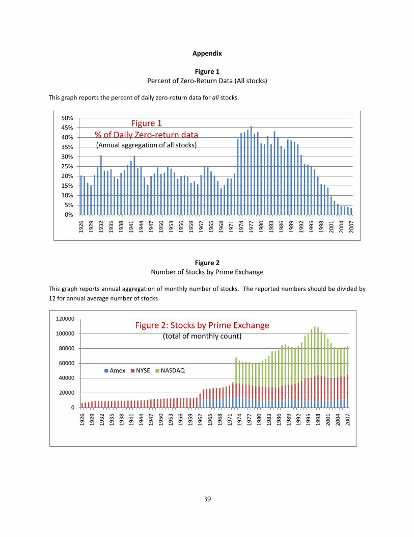
39

Appendix

Figure 1 Percent of Zero-Return Data (All stocks)

This graph reports the percent of daily zero-return data for all stocks.

Figure 2

Number of Stocks by Prime Exchange

This graph reports annual aggregation of monthly number of stocks. The reported numbers should be divided by 12 for annual average number of stocks

0%5%

10%15%20%25%30%35%40%45%50%

1926

1929

1932

1935

1938

1941

1944

1947

1950

1953

1956

1959

1962

1965

1968

1971

1974

1977

1980

1983

1986

1989

1992

1995

1998

2001

2004

2007

Figure 1% of Daily Zero-return data(Annual aggregation of all stocks)

0

20000

40000

60000

80000

100000

120000

1926

1929

1932

1935

1938

1941

1944

1947

1950

1953

1956

1959

1962

1965

1968

1971

1974

1977

1980

1983

1986

1989

1992

1995

1998

2001

2004

2007

Figure 2: Stocks by Prime Exchange(total of monthly count)

Amex NYSE NASDAQ

40

Figure 3 Percent of Zero-Return Data (Micro-cap stocks)

This graph reports the percent of daily zero-return data by four stock groups: Micro-cap, Large-cap (“sp”), Dow Jones Index (“dj”), and electricity stocks (“elect”) on a quarterly basis.

Figure 4

Percent of Zero-Return Data by Stock Group

This graph reports Percent of Zero-Return Data for four stock groups. The reported numbers are quarterly averages of daily percent of zero-return data.

0%

5%

10%

15%

20%

25%

30%

35%

40%

Dat

e7/

19/1

991

2/5/

1992

8/24

/199

23/

12/1

993

9/29

/199

34/

18/1

994

11/3

/199

45/

24/1

995

12/1

1/19

956/

28/1

996

1/16

/199

78/

5/19

972/

24/1

998

9/11

/199

84/

1/19

9910

/19/

1999

5/8/

2000

11/2

2/20

006/

14/2

001

1/8/

2002

7/29

/200

22/

14/2

003

9/4/

2003

3/24

/200

410

/12/

2004

5/2/

2005

11/1

6/20

056/

8/20

0612

/26/

2006

7/18

/200

7

Figure 3% of daily zero-retun data

Micro-cap stocks(Daily aggragation, 1991-2007)

41

Chapter 2

Factor Loadings and Model Predictions

This chapter presents the results of time-series tests of the CAPM and the Fama-French 3-factor (FF3) model in risk premium predictions of individual stocks and the Fama-French (FF) portfolios.

Section 1 tests for factor loadings of the CAPM and the FF3 model on individual stocks and the FF portfolios. Section 2 evaluates the main test of this paper, the inter-temporal and cross-sectional equivalence of the predicted returns of the CAPM and the FF3 model on individual stocks and the FF portfolios. Section 3 tests out-of-sample forecasts of the two models based on rolling regressions.

The regression test shows that the market index is the most consistently significant risk factor loading in both the CAPM and the FF3 model specifications on both individual stocks and the FF portfolios. The statistical power of the market index of individual stocks has inter-temporally increased, particularly for micro-cap stocks. This finding is robust, and contrasts with Fama-French (1992) who find little or no explanatory power of the CAPM beta in the cross-section of stock returns of the Fama-French portfolios, sorted on market capitalization and book-to-market ratio. The null hypothesis, the main test of this paper, that model-predicted risk premia of the CAPM and the FF3 model are statistically equal is not rejected for individual stocks. On the other hand, the FF3-predicted returns for the FF25 portfolios outperform the CAPM predictions. The regression tests on the factor loadings underline the similarities and dissimilarities of the CAPM and the FF3 model on individual stocks and the FF portfolios. The most intriguing finding on risk factor loadings is that the market index is no longer significant by itself for the Fama-French 25 portfolios within the FF3 model. Within the FF3 model, the market index loadings of the FF25 portfolios become significant in combination with SMB, HML, or both, but not alone. The turnabout is a stark contrast with the evidence that the market beta is more significant by itself for the majority of individual stocks in the FF3 model than in combination with other two factors. The turnabout is intriguing in that the market index loadings are statistically significant for every regression for all FF25 portfolios in the FF3 model in combination with SMB, HML, or both. It’s even more intriguing that the CAPM betas also are statistically significant for every regression for all FF25 portfolios; the CAPM beta is not always significant for all individual regressions, however. It’s puzzling that SMB and HML are not significant by itself or in combination with each other for any FF portfolios, but become as nearly significant as the market index when combined with the market index for the FF25 portfolios. For the FF25 portfolios, no factor is significant by itself, but factors become highly significant only in combination with the market index. A risk factor becomes significant in combination with other factor for the FF25 portfolios within the FF3 model.

42

The test of out-of-sample forecast using 5-year rolling regressions on monthly stock returns confirms the major findings of the test using daily data and conditioning information. For individual stocks, the mean squared errors (MSEs) of the out-of-sample forecast of the CAPM and the FF3 model are statistically equal. But the MSEs for the FF25 portfolios are not; for about half of the MSEs are statistically unequal. Nonetheless, the market index is the most consistently significant risk factor for both individual stocks and the FF portfolios.

The CAPM and the FF3 model in general are statistically equivalent in explaining individual stock returns. However, the two models are diametric in explaining the FF25 portfolios. The CAPM best explains large/growth (LG) portfolio returns, but is poor in explaining small/value (SV) portfolios. The high explanatory power of the CAPM for all LG portfolios is consistent, and so is the poor explanatory power for SV portfolios. The distinctive explanatory power of the CAPM between a large and growth portfolio and a small and value portfolio is clear and unambiguous, and is consistent with the CAPM or the market model. On the other hand, the FF3 model best explains small/value (SV) portfolios, a direct opposite of the CAPM. The FF3 model is most poor in explaining large/value (LV), not LG portfolios. In the FF3 model, the “value” portfolios are at both extremes in explaining power. Unlike the CAPM, most growth portfolios are located in the middle of the rank-order in the FF3 model. The virtual diametrical dissimilarities in explanatory power between the CAPM and the FF3 model for the FF25 portfolio and the statistical equivalence of the two models for individual stocks underline the unique structures of the FF portfolios and the two risk factors (SMB and HML). The factor structure of the FF25 portfolios appears to induce statistically significant factor loadings of SMB and HML, which are constructed based on the FF25 portfolio return structure that the two factors explain.

43

1. Risk Factor Loadings55

The regression tests show that the CAPM beta is the most consistently significant risk factor

loading among the three factors. The regression tests also reveal and magnify the similar and dissimilar

patterns in the factor loadings of the CAPM and the FF3 model when the models are applied on two

different groups of returns: individual stock returns and the FF portfolio returns. For individual stocks,

the market index in the FF3 model is the most significant factor loading alone or in combination with

other factors. For the FF portfolios in the FF3 model, the market index also is the most significant factor,

but in combination with SMB and HML, not alone. (Tables 1-1-1 and 1-1-2)

A. Model Specification Tests

The most intriguing finding on the risk factor loadings is that the market index is no longer

significant by itself for the Fama-French 25 portfolios within the FF3 mode. Within the FF3 model, the

market index loadings of the FF25 portfolios become significant in combination with SMB, HML, or

both, but not alone. (Panel B of Tables 1-1-1 and 1-1-2)

a. Significance of Risk Factor Loadings

The table below is a condensed summary of Tables 1-1-1 and 1-1-2 on the percentage of a

combination of significant factor loadings. For large-cap stocks, the market index is a significant factor

loading by itself (Specification 1) for 43.1 percent of annual regressions and 58.9 percent of quarterly

regressions in the FF3 model. For all individual stock groups and the FF12 industry portfolios, the

market index is the most significant factor loading in the quarterly estimations (Specification 1).

However, the picture changes for the FF portfolios. The market index no longer is a single factor

significant by itself in the FF portfolios. The return structure for the FF portfolios is highly predictable.

For the FF10ME portfolios, the market index and SMB jointly are significant (Specification 2). For the

FF10BM portfolios, the market index and HML jointly are significant (Specification 4). For the FF25

portfolios, three risk factors jointly are significant (Specification 3). The market index is most significant

for every FF portfolio in combination with other factor, but not by itself.

55 For brevity, unless specifically referred to a model, size, etc., each sentence applies generally to both models, to all groups of stocks, and to all categories.

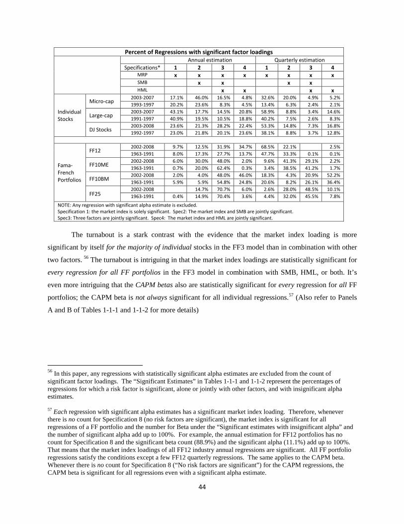
44

Percent of Regressions with significant factor loadings Annual estimation Quarterly estimation

Specifications* 1 2 3 4 1 2 3 4 MRP x x x x x x x x SMB x x x x HML x x x x

Individual Stocks

Micro-cap 2003-2007 17.1% 46.0% 16.5% 4.8% 32.6% 20.0% 4.9% 5.2% 1993-1997 20.2% 23.6% 8.3% 4.5% 13.4% 6.3% 2.4% 2.1%

Large-cap 2003-2007 43.1% 17.7% 14.5% 20.8% 58.9% 8.8% 3.4% 14.6% 1991-1997 40.9% 19.5% 10.5% 18.8% 40.2% 7.5% 2.6% 8.3%

DJ Stocks 2003-2008 23.6% 21.3% 28.2% 22.4% 53.3% 14.8% 7.3% 16.8% 1992-1997 23.0% 21.8% 20.1% 23.6% 38.1% 8.8% 3.7% 12.8%

Fama-French Portfolios

FF12 2002-2008 9.7% 12.5% 31.9% 34.7% 68.5% 22.1% 2.5% 1963-1991 8.0% 17.3% 27.7% 13.7% 47.7% 33.3% 0.1% 0.1%

FF10ME 2002-2008 6.0% 30.0% 48.0% 2.0% 9.6% 41.3% 29.1% 2.2% 1963-1991 0.7% 20.0% 62.4% 0.3% 3.4% 38.5% 41.2% 1.7%

FF10BM 2002-2008 2.0% 4.0% 48.0% 46.0% 18.3% 4.3% 20.9% 52.2% 1963-1991 5.9% 5.9% 54.8% 24.8% 20.6% 8.2% 26.1% 36.4%

FF25 2002-2008 14.7% 70.7% 6.0% 2.6% 28.0% 48.5% 10.1% 1963-1991 0.4% 14.9% 70.4% 3.6% 4.4% 32.0% 45.5% 7.8%

NOTE: Any regression with significant alpha estimate is excluded. Specification 1: the market index is solely significant. Spec2: The market index and SMB are jointly significant. Spec3: Three factors are jointly significant. Spec4: The market index and HML are jointly significant.

The turnabout is a stark contrast with the evidence that the market index loading is more

significant by itself for the majority of individual stocks in the FF3 model than in combination with other

two factors. 56 The turnabout is intriguing in that the market index loadings are statistically significant for

every regression for all FF portfolios in the FF3 model in combination with SMB, HML, or both. It’s

even more intriguing that the CAPM betas also are statistically significant for every regression for all FF

portfolios; the CAPM beta is not always significant for all individual regressions.57

56 In this paper, any regressions with statistically significant alpha estimates are excluded from the count of significant factor loadings. The “Significant Estimates” in Tables 1-1-1 and 1-1-2 represent the percentages of regressions for which a risk factor is significant, alone or jointly with other factors, and with insignificant alpha estimates. 57 Each regression with significant alpha estimates has a significant market index loading. Therefore, whenever there is no count for Specification 8 (no risk factors are significant), the market index is significant for all regressions of a FF portfolio and the number for Beta under the “Significant estimates with insignificant alpha” and the number of significant alpha add up to 100%. For example, the annual estimation for FF12 portfolios has no count for Specification 8 and the significant beta count (88.9%) and the significant alpha (11.1%) add up to 100%. That means that the market index loadings of all FF12 industry annual regressions are significant. All FF portfolio regressions satisfy the conditions except a few FF12 quarterly regressions. The same applies to the CAPM beta. Whenever there is no count for Specification 8 (“No risk factors are significant”) for the CAPM regressions, the CAPM beta is significant for all regressions even with a significant alpha estimate.

(Also refer to Panels

A and B of Tables 1-1-1 and 1-1-2 for more details)

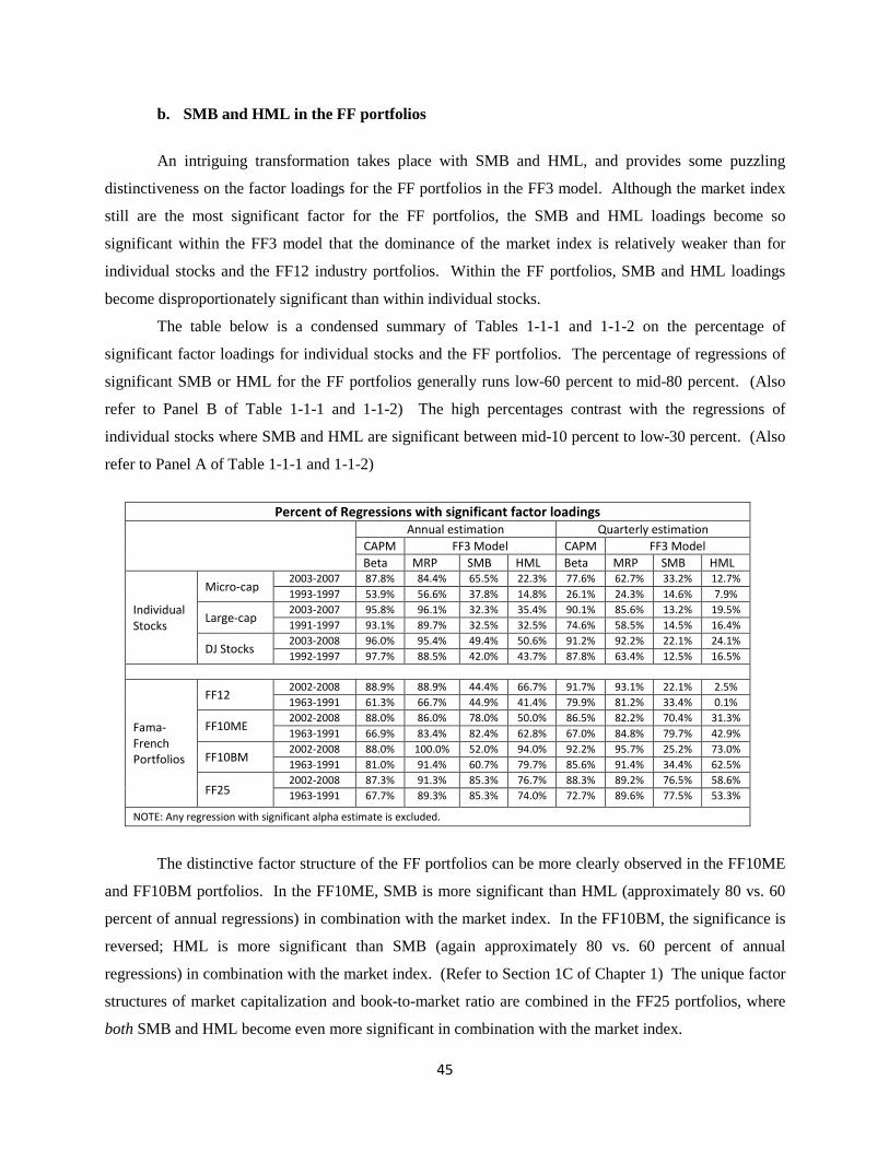
45

b. SMB and HML in the FF portfolios

An intriguing transformation takes place with SMB and HML, and provides some puzzling

distinctiveness on the factor loadings for the FF portfolios in the FF3 model. Although the market index

still are the most significant factor for the FF portfolios, the SMB and HML loadings become so

significant within the FF3 model that the dominance of the market index is relatively weaker than for

individual stocks and the FF12 industry portfolios. Within the FF portfolios, SMB and HML loadings

become disproportionately significant than within individual stocks.

The table below is a condensed summary of Tables 1-1-1 and 1-1-2 on the percentage of

significant factor loadings for individual stocks and the FF portfolios. The percentage of regressions of

significant SMB or HML for the FF portfolios generally runs low-60 percent to mid-80 percent. (Also

refer to Panel B of Table 1-1-1 and 1-1-2) The high percentages contrast with the regressions of

individual stocks where SMB and HML are significant between mid-10 percent to low-30 percent. (Also

refer to Panel A of Table 1-1-1 and 1-1-2)

Percent of Regressions with significant factor loadings

Annual estimation Quarterly estimation CAPM FF3 Model CAPM FF3 Model Beta MRP SMB HML Beta MRP SMB HML

Individual Stocks

Micro-cap 2003-2007 87.8% 84.4% 65.5% 22.3% 77.6% 62.7% 33.2% 12.7% 1993-1997 53.9% 56.6% 37.8% 14.8% 26.1% 24.3% 14.6% 7.9%

Large-cap 2003-2007 95.8% 96.1% 32.3% 35.4% 90.1% 85.6% 13.2% 19.5% 1991-1997 93.1% 89.7% 32.5% 32.5% 74.6% 58.5% 14.5% 16.4%

DJ Stocks 2003-2008 96.0% 95.4% 49.4% 50.6% 91.2% 92.2% 22.1% 24.1% 1992-1997 97.7% 88.5% 42.0% 43.7% 87.8% 63.4% 12.5% 16.5%

Fama-French Portfolios

FF12 2002-2008 88.9% 88.9% 44.4% 66.7% 91.7% 93.1% 22.1% 2.5% 1963-1991 61.3% 66.7% 44.9% 41.4% 79.9% 81.2% 33.4% 0.1%

FF10ME 2002-2008 88.0% 86.0% 78.0% 50.0% 86.5% 82.2% 70.4% 31.3% 1963-1991 66.9% 83.4% 82.4% 62.8% 67.0% 84.8% 79.7% 42.9%

FF10BM 2002-2008 88.0% 100.0% 52.0% 94.0% 92.2% 95.7% 25.2% 73.0% 1963-1991 81.0% 91.4% 60.7% 79.7% 85.6% 91.4% 34.4% 62.5%

FF25 2002-2008 87.3% 91.3% 85.3% 76.7% 88.3% 89.2% 76.5% 58.6% 1963-1991 67.7% 89.3% 85.3% 74.0% 72.7% 89.6% 77.5% 53.3%

NOTE: Any regression with significant alpha estimate is excluded.

The distinctive factor structure of the FF portfolios can be more clearly observed in the FF10ME

and FF10BM portfolios. In the FF10ME, SMB is more significant than HML (approximately 80 vs. 60

percent of annual regressions) in combination with the market index. In the FF10BM, the significance is

reversed; HML is more significant than SMB (again approximately 80 vs. 60 percent of annual

regressions) in combination with the market index. (Refer to Section 1C of Chapter 1) The unique factor

structures of market capitalization and book-to-market ratio are combined in the FF25 portfolios, where

both SMB and HML become even more significant in combination with the market index.

46

It’s puzzling that SMB and HML is insignificant by itself or in combination with each other for

all FF portfolios, while the two factors are significant in combination with each other for some individual

stocks. For the FF portfolios, SMB or HML is insignificant by itself or in combination with each other,

but becomes highly significant only in combination with the market index. However, when combined

with the market index, the two factors become as nearly significant as the market index for more than

three quarters of annual regressions in the FF3 model. (Panels A and B of Tables 1-1-1 and 1-1-2) A

similar pattern is also found for two types of Fama-French portfolios: the FF10ME sorted on market

capitalization and the FF10BM sorted on book-to-market ratio. None of three risk factors generally is

significant by itself for the FF10ME and the FF10BM portfolio returns within the FF3 model. (Panel B of

Tables 1-1-1 and 1-1-2) All three factors, when combined, are significant for the FF25 portfolios in the

FF3 model.

Grout and Zalewska (GZ, 2006, pp.152, 176) also find that the impact of SMB and HML is less

clear than that of the market factor; the factors do not seem to provide extra explanatory power. GZ find

that the effect of the two factors is significant through the market factor.

The above distinctive factor structure of the FF portfolios suggest that a test result of the FF3

model on the FF portfolios is an artifact of portfolio formation and the two factor construction. SMB and

HML are constructed by the portfolio returns, which the two factors are supposed to explain as

recognized in FF (1993, p.8). Van Horne (2001, p.75) argues that regression tests of the portfolios sorted

on market-cap size and book-to-market value on SMB and HML which are also formed on market-cap

size and book-to-market value would produce statistically more significant results than otherwise.

It’s also notable that the CAPM beta and the FF3 model market index loadings in general are

equally significant for individual stocks and the FF12 industry portfolios. (Also refer to Panel A of Table

1-1-1 and Table 1-1-2) When the significance of the market index loadings increased during the test

period (for example, micro-cap stocks and the FF12 industry portfolios), the significance of the factor

loadings of both models moved up virtually in lock-step. By the end of the test period (2003-2008), the

percentages of the significant CAPM betas for the FF portfolios in general have become virtually

identical to those of the FF3 model market index loadings. In the FF portfolios, the percentages of

significant market index for both models also are high, ranging between 80 and 90 percent. (Also refer to

Panel B of Table 1-1-1 and 1-1-2)

c. Alpha estimates

The FF portfolios appear to induce mispricing by construction. The FF portfolios have larger

numbers of regressions with significant alpha estimates than individual stocks. The table below is a

47

condensed summary of Tables 1-1-1 and 1-1-2, and reports the percentages of regressions that have the

highest number of significant alpha estimates in the individual stock groups and the FF portfolios.

Regressions with Largest Number of Significant Alpha Estimates (%) Individual Stocks Fama-French Portfolios 1991-2008* 1992-2008 1963-1991 Annual

estimation Quarterly

estimation Annual

estimation Quarterly

estimation Annual

estimation Quarterly

estimation CAPM 4.7% 5.9% 26.4% 24.0% 38.7% 33.0% FF3 Model 5.2% 4.4% 16.7% 17.8% 33.3% 18.7% NOTE: Individual stocks cover different period between 1991 and 2008 as reported in Tables 1-1-1 and 1-1-2

The percentages of statistically significant alpha estimates of both models for individual stocks

are at 5.9 percent or lower across stock groups and between annual and quarterly estimations.58 (Also

refer to Panel A of Tables 1-1-1 and 1-1-2) However, the percentages for the FF portfolios are as four

times high as those of individual stocks for the corresponding period, 1992-2008.59

58 Regressions with significant alpha estimates and insignificant alpha estimates are counted mutually exclusively in this paper. Any regression with significant alpha is included in the count of “statistically significant alpha estimates” regardless of statistical significance of any factor loadings, and also excluded from the count of “Significant factor loadings.” 59 Hu (2007, p.125) reports significant alpha estimates of the Fama-French 3-factor model. The main reason for the serious, positive, and significant alpha estimates may be a result of the research method. Hu estimates the “expected” risk factor premia of the Fama-French 3 risk factors using “structural variables” as explanatory factors. The adjusted R2 of the regressions to estimate the “expected” risk premia are a low 0.04. The “expected” risk factor premia then are used as explanatory variables for the risk premia of “no investment” trading portfolios that are formed out of 17 industry portfolios. The trading portfolios are reallocated every month and so are the “no investment” trading portfolios. The final estimate process relates the “no investment” trading portfolios and the “expected” three Fama-French factor premia. The test process risks the pitfalls related with the estimation of expected risk premia (Merton, 1980) and the regular portfolio allocation (FF, 2007a, 2007b, 2008) as discussed in Chapter 1.

(Also refer to Panel B

of Tables 1-1-1 and 1-1-2) The percentages are much higher for the period of 1963-1991.

It’s notable that the significant alpha estimates for the FF25 portfolios remain largely unchanged:

8.7 percent in annual estimation and 10.8 percent in quarterly estimation in 2003-2008 vs. 10.7 and 10.4

percent respectively in 1963-1991. (Panel B of Tables 1-1-1 and 1-1-2)

The higher numbers of statistically significant alpha estimates of the FF portfolios than those of

individual stocks suggest that mispricing of the FF3 model for the FF portfolios is more serious than for

individual stocks. At the same time, the low and similar percentages of the numbers of significant alpha

estimates between the two models for individual stocks and the FF12 industry portfolios suggest that the

contributions from the FF3 model to the CAPM beta would be rather marginal for individual stocks and

the FF12 industry portfolios.

48

d. Regressions of No Significant Loadings and Alpha60

The FF portfolios and individual stocks have opposite characteristics on the significant alpha

estimates and the regressions with no significant factor loading. For the alpha estimates, individual stock

regressions are superior as discussed in the previous subsection. However, individual stocks have higher

percentages of regressions with no significant risk factor loading than the FF portfolios. For the

significance of factor loadings, the FF portfolios are superior; every FF portfolio regression has a

significant factor loading. It’s remarkable that the market index is significant for all regressions of all FF

portfolios in the FF3 model. (Tables 1-1-1 and 1-1-2 and the Exhibits to Tables 1-1)

The table below is a condensed summary of the percentages of regressions with no significant

factor loadings. Individual stocks with insignificant factor loadings have dramatically dropped during the

test period. For example, the percentage of annual regressions for micro-cap stocks dropped from 33.4

percent in 1993-1997 to 8.1 percent in 2003-2007 in the FF3 model; the quarterly regressions make a

remarkable change from 65 percent down to 23 percent. (Also refer to Panel A of Tables 1-1-1 and 1-1-

2) Large-cap and Dow Jones Index stocks also improved in the FF3 model, albeit to a less degree: from

29.9 percent down to 8.5 percent for large-cap and from 33.0 percent to 3.6 percent for Dow Jones Index

stocks in the quarterly regressions between the two subsample periods. It’s particularly notable that

approximately 75 percent of quarterly regressions of micro-cap stocks had no significant factor loadings

in the FF3 model in 1993. Since then, the percentage made a dramatic drop of more than 60 percentage

points during the test period, down to close to 10 percent. (Refer to Exhibits to Tables 1-1) These

dramatic changes appear consistent with the steady improvement of zero-return data discussed in Section

1 of this chapter.

Percent of regressions with no significant factor loadings Annual regressions Quarterly regressions Micro-cap Large-cap DJ Stocks Micro-cap Large-cap DJ Stocks

2003-2007 CAPM 7.6% 0.1% 18.3% 5.7% 2.9%

FF3 8.1% 0.2% 22.9% 8.5% 3.6%

1992-1997 CAPM 42.7% 3.4% 71.5% 23.0% 9.6%

FF3 33.4% 2.6% 6.3% 64.9% 29.9% 33.0%

NOTE: Every FF portfolio regressions has at least a significant factor loading, except the quarterly regressions of the FF12 industry portfolios

60 The “Regressions of No Significant Loadings and Alpha” or Specification 8 is one of eight specifications where all alpha estimates are insignificant.

49

e. Time-invariance of Factor Loadings of FF25 Portfolios

The FF25 portfolios show a distinct factor loading characteristic within the FF3 model; the

significance of the factor loadings has remained largely time-invariant throughout the entire period, 1963-

2008. In the CAPM, the market beta for both individual stocks and the FF3 portfolios increasingly

became significant during the test period, and subsequently the number of regressions where no risk

factor is statistically insignificant decreased. In the FF3 model, the market index loadings for individual

stocks and the FF12 industry portfolios also increasingly became significant during the test period, while

that of FF25 portfolios in the FF3 model remained largely time-invariant during the entire period, 1963-

2008. (Table 1-1-1 and 1-1-2 and Exhibits to Tables 1-1)

The relative time-invariance of the FF25 portfolio factor loadings contrasts with individual stocks

and the FF12 industry portfolios, which in general made inter-temporal increases in the significance of the

CAPM beta or the market index loadings. The factor loadings of the FF10ME and FF10BM portfolios

show similar tendency of time-invariance, albeit to a less degree.

The increases in the significance of factor loadings are most conspicuous for micro-cap stocks,

consistent with the most dramatic decreases in zero-return data for micro-cap stocks as discussed in

Chapter 1. The significance of the market index by itself and in combination with SMB and HML for

micro-cap stocks increased from approximately 50 percent of annual estimations in the beginning of the

test period to approximately 90 percent in 2007, and from 20 percent of quarterly estimations in the

beginning of the test period to 70 percent in 2007. (Exhibits to Tables 1-1) The improvement was

followed by the decreases in regressions where all risk factors are insignificant; those regressions dropped

from approximately 40 percent of annual estimations in the beginning of the test period to approximately

less than 10 percent in 2007, and from 70 percent of quarterly estimations in the beginning of the test

period to approximately 10 percent in 2007, an astounding 60 percentage point decrease. The steady

increase in the significance of the market beta and the dramatic decreases in regressions with no

significant load factors suggest that the CAPM beta increasingly have become reliable and relevant as the

market risk, particularly for micro-cap stocks.

On the other hand, the significance of the factor loadings of the FF25 portfolios has remained

relatively stable in spite of a large decline of zero-return data beginning in the early 1990s. The relative

stability is deemed unusual because the significance of factor loadings of the FF portfolios sorted on

either capitalization or book-to-market ratio have shown some improvement. It’s intriguing that every FF

portfolio has at least a significant factor loading throughout the entire period 1963-2008, except the

quarterly regressions of the FF12 industry portfolios. Even more intriguing is that the risk factor

50

significant for all FF portfolios is none other than the market index. It appears that the methods of the

FF25 portfolio formation and the two risk-factor construction in the FF3 model make the FF25 portfolios

in the FF3 model remain relatively unperturbed by external forces.

B. Regression Diagnostics

Regression diagnostics confirm the findings on the factor loadings. For individual stocks, the

statistics of two models are largely equivalent. For the FF portfolios, the FF3 model is clearly superior.

Inter-temporally, the CAPM statistics steadily improved while the FF3 model statistics remained largely

time-invariant.

An F-test for omitted variables adds more evidence on the dissimilarities of the FF portfolio from

individual stocks. The test on individual stocks shows that the contributions of the market index to SMB

and HML are overwhelming compared to those of SMB and HML to the market index. (Table 1-2-1) The

market index almost always adds to SMB and HML while the two variables add to the market index

much less often. The contribution rates on a quarterly basis drops from those on an annual basis;

however, the market index still makes higher contributions than those made by SMB and HML combined.

It’s notable that the contributions for micro-cap stocks have steadily increased with the contributions of

the market index growing faster than those of other two factors. The steady increase in significance of the

risk factor for micro-cap stocks appear to be consistent with the steady decrease in zero-return data.

The F-test for omitted variables on the Fama-French portfolios also confirms the findings in the

model specification tests: the market index adds to SMB and HML for all FF portfolios on an annual and

quarterly basis. (Table 1-2-1) SMB adds mostly to the FF10ME sorted on market capitalization, much

less to the FF10BM sorted on book-to-market ratio. The opposite happens with HML; HML largely adds

to the FF10BM, except much less to the FF10ME. The FF25 portfolios again show a unique

characteristic. The market index makes contribution to all 25 portfolios on an annual basis throughout the

entire period. So do SMB and HML, except for a few years for a few portfolios in the 1970s. On a

quarterly basis, the market index also makes contribution to all 25 portfolios. SMB and HML jointly

make contribution to all portfolios, but except six large capitalization portfolios: s4h2 (84%), s4h3 (86%),

s4h4 (87%), s4h5 (87%), s5h2 (69%), and s5h3 (78%). These six portfolios that failed to make a 100%

contribution show no consistent temporal concentrations or patterns, consistent with the evidence that the

FF3 model is relatively poor in explaining large capitalization portfolios.

Residual tests for serial correlations and heteroskedasticity show a contrast between individual

stocks and the FF portfolios. The CAPM residuals are slightly less serially-correlated and heteroskadastic

for individual stocks than the FF3 model residuals. (Table 1-2-2) But the pattern becomes reversed for

the FF25 portfolios; the CAPM residuals are more serially-correlated and heteroskadastic. For example,

51

the percentages of annual regressions with no serial correlations and heteroskedasticity of large-cap

residuals are 71.5% for the CAPM and 66.7% for the FF3 model. However, the percentages are reversed

for the FF25 portfolios, 32.2% vs. 51.5%. These contrasting patterns between the CAPM and the FF3

model on individual stocks and the FF portfolios are repeated for the quarterly regression residuals. The

reversal may indicate that tests on individual stocks and the FF portfolios are not comparable because of a

unique combination of the FF portfolio formation method and the two factor construction.

The inter-temporal changes of regression residuals add more insight. For individual stocks, both

models show fairly similar residual patterns for each year. (The accompanying figures to Table 1-2-2)

For micro-cap stocks, both model residuals show steady increases in non-serial correlations and non-

heteroskedasticity. However, for the FF25 portfolios, the CAPM and the FF3 model residuals show

contrasting patterns. The CAPM residuals have steadily improved throughout the test period, and became

closer to the FF3 model residuals. However, the FF3 model residuals show no clear upward trend. The

inter-temporal invariance of the residuals of the FF3 model may be a result of a unique combination of the

FF portfolio formation method and the two factor construction. Because of a different method of

portfolio formation, the FF12 industry portfolios add additional evidence on the plausible sources of the

difference of the CAPM and the FF3 model on individual stocks and the FF portfolios.

The CAPM and the FF3 model also show dissimilar characteristics in regression statistics. (Table

1-3 and Figure 2-1) The R2 and the variations of the CAPM and the FF3 model move or change largely

in tandem for individual stocks. The adjusted R2 of the FF3 model are consistently higher than the

CAPM, an indication of some information content of SMB and HML. For the FF25 portfolios, on the

other hand, the adjusted R2 of the FF3 model are far superior to those of the CAPM. In addition, the

variations of the FF3 model are much lower and more stable than those of the CAPM. A similar pattern

is also observed in the Schwartz Bayesian Criteria (SBC). The SBC’s of the FF3 model for the FF25

portfolios are far more superior to the CAPM than they are for individual stocks. However, no such

pattern is observed on the FF12 industry portfolios. Similar to individual stocks but unlike the FF25

portfolios, the R2 and the variations of the CAPM and the FF3 model also move or change largely in

tandem for the FF12 industry portfolios. Again, similar to individual stocks but unlike the FF25

portfolios, the SBC’s of the CAPM and the FF3 model for the FF12 industry portfolios are close to each

other.

For individual stocks, the CAPM explains practically an equal number of annual regressions as

the FF3 model, or even larger numbers of quarterly regressions. However, the pattern is reversed for the

FF25 portfolios. The FF3 model explains far larger numbers of regressions for the FF25 portfolios than

the CAPM, consistent with the findings for the model specification tests. The FF12 industry portfolios

again are more similar to individual stocks than to the FF25 portfolios in this regard.

52

The CAPM betas and the FF3 model market index loadings are similarly variable for individual

stocks and the FF25 portfolios. However, the beta estimates of the FF3 model for the FF25 portfolios are

a virtual unity with much less variations. In addition, the variations in the market index loadings and the

alpha estimates of the FF3 model for the FF25 portfolios is consistently lower or more stable than those

of the CAPM. On the other hand, no such consistent and clear patterns are observed for individual stocks

and the FF12 industry portfolios. The findings add evidence that the FF portfolios are artifacts of a

unique portfolio formation and the two factor construction.

2. Model-predicted Risk Premium

The main test or Hypothesis 1 of this paper concerns how closely the model-predicted risk premia

(PRP) are correlated with the realized risk premia (RRP) as specified in Equation 3. This test based on

Equation 3 facilitates direct and consistent comparisons of the CAPM with the FF3 model. To the end,

this paper estimates the temporal correlations between the PRP and the RRP for each firm over the test

period, and assesses the estimation reliability of the two models.

The model-predicted risk premium test results are a virtual repeat of what have already been

found in the factor loadings discussed in the previous section of this chapter. For individual stocks, the

predicted risk premia of the CAPM and the FF3 model largely are statistically equivalent. This general

result is expected because the market index is not only the common risk factor of both models, and also

the most significant risk factor loading among three factors. The market index is the dominant systematic

risk factor among the three factors.

However, the FF3 model predictions are superior under the following three circumstances: during

high market volatility, the model-predicted returns for the FF25 portfolios, and the annual estimations of

micro-cap stocks.

Tables 2-1 through 2-3 present the test results for six stock groups: micro-cap, large-cap, Dow

Jones 29 stocks, the electric power industry firm stocks, Fama-French 12 industry portfolios, and 25

portfolios. The tables present multi-dimensional test results: (1) by estimation interval (annual, quarterly,

and monthly), (2) by test subsample (Full test period, Period 1 through 1997, Period 2 for 1998-2002, and

Period 3 for 2003-2007 for micro-cap and large-cap stocks; Period 1 for 1963-1972, Period 2 for 1973-

1990, Period 3 for 1991-2000, and Period 4 for 2001-2008 for Fama-French portfolios), (3) by statistical

significance and the direction of the correlations (positive or negative) of the model-predicted returns and

the realized returns, and (4) by model. The statistical test estimates the correlations of the PRP of each

model with the RRP, and compares the number of significant correlations of the two models.

53

A. Large-cap and Dow Jones Index Stocks

The return predictions of both the CAPM and the FF3 model for large-cap and Dow Jones Index

stocks are largely equal in both the number of firms with statistically significant correlations of PRP with

the RRP and in the significant correlation coefficients between the PRP and the RRP. (Tables 2-1) For

Dow Jones Index stocks, the correlations of the CAPM-predicted returns with the RRP are somewhat

higher than those of the FF3 model. The statistical equality of the two model-predicted returns for the

two stock groups suggests that the CAPM and the FF3 model can be equally useful in the estimation of

the cost of capital.

However, market volatility significantly affects systematic risk measurement for annual

estimation of both models. Only 20 percent of Dow Jones Index stock PRPs and eight percent of large-

cap stock PRPs have statistically significant annual estimation for 1998-2002. Micro-cap stocks and the

electric power stocks show far worse patterns. For micro-cap stocks, only two percent of PRPs of the

CAPM annual estimation and 6 percent of the FF3 model are significant. Market volatility affects

systematic risk measurement of the CAPM more than that of the FF3 model. Additional insight is that

market volatilities become more serious for longer-interval or annual estimations for all individual stock

groups; little impact of market volatilities is observed for quarterly or monthly estimations. This finding

further corroborates the non-stationarity of systematic risk and the beta-shift over time. The finding

further reinforces the importance of measuring systematic risk and risk factor loading based on

conditioning information, rather than at fixed estimation intervals such as 5-year intervals regardless of

the economic and market conditions.

Although the two model-predicted risk premia are statistically equal for individual stocks, the test

results vary for estimation intervals - annual, quarterly, or monthly estimation - and also for test time

lengths – the full test period or subsample periods. The varying test results make the conclusions and

interpretations on the test results something of a challenge. The number of significant correlations of PRP

and RRP is a negative function of estimation intervals for both models. For example, a large number of

model-predicted returns are significantly correlated with RRP for monthly estimation but the number

drops as the estimation interval becomes longer. More than 90 percent of Dow Jones Index PRP is

significant for monthly estimation, which drops monotonically as estimation interval becomes longer.

The inverse relation also is true for the large-cap PRP; more than 80 percent PRP are significant for

monthly estimation, which also drops monotonically as estimation interval becomes longer. On the other

hand, the correlations of PRP are a positive function of estimation interval also for both models. The

correlations of Dow Jones Index PRP for monthly estimation are in a 0.5 range, which monotonically

increase with the length of estimation interval, reaching a 0.9 range for annual estimations. The opposite

54

directions of the relations also are found in micro-cap and electric power stocks. Further research on the

factor loading generating process is warranted.

The negative relations of PRP with the estimation intervals may suggest non-stationary

systematic risks. The positive relations of correlations may indicate that stocks highly correlated with the

systematic risk also retain statistical stability and significance for varying lengths of estimation interval.

These findings may suggest that firms less correlated with the systematic risk use shorter estimation

interval but firms highly correlated with the systematic risk may use a longer estimation interval. The

interpretation seems reasonable and intuitive. Stock returns that are highly correlated with systematic risk

generally may have a lower percentage of trading days with high noise or idiosyncratic volatilities over a

longer estimation interval than a shorter interval. On the other hand, the opposite generally may be true

with stock returns weakly correlated with systematic risk. Further research on the factor loading

generating process is warranted.

B. Micro-cap and Electric Power Stocks

The FF3 model-predicted risk premia for micro-cap are superior in the number of significant

stocks. (Table 2-2) However, the correlation coefficients of the significant PRP stocks largely are equal

between the CAPM and the FF3 model. The relative superiority of the FF3 in PRP is consistent with the

findings of the previous section on the low percentage of significant market factor loadings of micro-cap

stocks. However, the predictive power of both the CAPM and the FF3 model for micro-cap stock returns

are weaker compared to those for large-cap or Dow Jones Index stocks. (Compare Table 2-1 vs. Table 2-

2)

The most distinctive and unique characteristic of micro-cap PRPs perhaps is that model-predicted

returns have become increasingly correlated with the realized returns over the test period. All three

estimation intervals show the consistent inter-temporal patterns. Unlike large-cap or DJ stocks, the PRPs

of micro-cap stocks during the first subsample (1993-1997) are even more weakly correlated with the

RRPs than during the high market volatility (1998-2002) for all estimation intervals. The powerful

impacts of non-synchronous or zero-return data may be underlined by the findings. Another unique

characteristic of micro-cap stocks is that the FF3 model-predicted PRP is superior for longer estimation

intervals (annual, quarterly vs. monthly) to the CAPM PRPs. It’s unclear why the FF3 model is superior

for longer estimation intervals and for micro-cap stocks.

The most distinctive and unique characteristic of the electric power stock PRPs perhaps is that,

for all estimation intervals, the CAPM is consistently inferior to the FF3 model during the second

subsample period (1998-2002). During this period, the industry simultaneously experienced its own

55

industry-wide and the market-wide volatilities in 1998-2002. Further research to separate the impacts of

two volatilities is warranted.

C. Fama-French Portfolios

The FF3 model is consistently superior to the CAPM for all estimation intervals and all

subsample periods in explaining the FF portfolios. The FF3 model predictions outperform the CAPM for

the FF portfolios. (Table 2-3-1)

More detailed findings on the portfolio return correlations and the factor loadings are as follows:

Unlike individual stock groups, all PRPs of the FF12 and FF25 portfolios are significant for all estimation

intervals and for both models, except for the annual estimation for 1992-2000 and 2001-2008; it’s unclear

why the two subsample periods of annual estimation are less significant. Unlike individual stock groups,

the correlations of PRPs of both models are high consistently for all estimation intervals and for both

models. The correlations of both model-predicted returns are mostly 0.8 or higher for the FF12 industry

portfolios; the predicted correlations for FF25 portfolios also are 0.8 or higher for the CAPM and 0.9 or

higher for the FF3 model. Unlike individual stock groups, the correlations of CAPM PRPs for the FF25

portfolios are lower than those of the FF3 model PRPs, consistently for all estimation intervals and all

subsample periods.

Nonetheless, the CAPM predictions are somewhat close to the FF3 model. First, The CAPM-

predicted risk premia are practically equal with the FF3 model in the number of significant estimation of

portfolio returns, except the annual estimation-based predictions in 1992-2000 and 2001-2008. The FF3

model predictions also deteriorated during the periods, albeit to a less degree. Second, the CAPM

predictions are as equally correlated with the realized risk premiums as the FF3 model predictions at

correlation coefficients of 0.8 or higher for the FF12 portfolios, similar to those of the FF3 model. The

correlations coefficients of the CAPM predictions are higher than those of the FF3 predictions for

individual stocks.

The above distinct and unique characteristics of Fama-French portfolio PRPs are expected and

consistent with the findings in this paper: Fama-French portfolio returns have higher correlations with all

three risk factors than individual stock groups. SMB and HML make more significant contributions to

the FF portfolios than to individual stock groups.

Table 2-3-2 reports a divergent characteristic between the CAPM and the FF3 model in

explaining the FF25 portfolios. When the correlations of the model-predicted risk premium of the FF25

portfolios with the realized risk premium are rank-ordered by the model, the CAPM best explains

large/growth (LG or large capitalization with low book-to-market ratio) portfolio returns, but is poor in

56

explaining small/value (SV) portfolios. The high explanatory power of the CAPM for all LG portfolios is

consistent, and so is the poor explanatory power for SV portfolios. The distinctive differences of

explanatory power of the CAPM between a large and growth (LG) portfolio and a small and value (SV)

portfolio are clear and unambiguous. However, the FF3 model best explains small/value (SV) portfolios,

which is a direct opposite of the CAPM. On the other hand, the FF3 model is most poor in explaining

large/value (LV), not large/growth. Unlike the CAPM, most growth portfolios are located in the middle

of the rank-order in the FF3 model. In the FF3 model, the explanatory power for “value” portfolios is at

both extremes.

The market value of large-cap stocks is 90 percent of the total market value while that of small-

cap stocks is 3 percent. (FF, 2008) The superiority of the CAPM in explaining large-cap growth stocks

and the inferiority of the FF3 model in explaining large-value growth may undermine the application

value of the FF3 model for the estimation of the cost of equity capital. Furthermore, the virtual

diametrical explanatory power between the CAPM and the FF3 model for the FF25 portfolio suggests that

a test of the CAPM on the FF25 portfolios is incompatible or incomparable with a test of the FF3 model

on the portfolios.

3. Out-of-sample Forecasts

The test results of out-of-sample, one-period-ahead forecasts of the CAPM and the FF3 model on

monthly returns enhance the robustness of the main findings of the tests that use daily return data and

conditioning information on the market and the economy. The consistent, main findings of the out-of-

sample forecasts of individual stock returns include: The one-period-ahead mean squared errors (MSEs)

of the two models mostly are statistically equal;61

61 A test for 12-month-ahead forecasts, not reported in this paper, indicates the statistical equality of the two models forecast MSEs.

the market index is the most consistent and significant

loading factor.

The test is conducted for 5-year rolling regressions of monthly returns of individual stocks. The

5-year rolling regressions start 1988-1992, and the one-period-ahead forecast begins January 1993. The

F-test results reported in Table 2-4-1 for the one-period-ahead MSEs of the CAPM and the FF3 model

corroborate the previous tests for the equivalency of the two model-predicted risk premia. The MSEs of

the two models are statistically equal, except for a few months in 2000 and 2001 when the market was

highly volatile. A caveat: the high variability of MSEs of micro-cap stocks may be the main reason for

statistical equality as indicated by the relatively poor SBCs, low R2, and weak t-statistics of the parameter

estimates compared to those of large-cap and Dow Jones Index stocks (See Table 2-4-5).

57

Table 2-4-2 reports the specifications of the rolling regressions, which also confirm the findings

of the previous tests on factor loadings and regression statistics. The market index is the most consistent

and significant factor loading among three risk factors. For large-cap and the Dow Jones Index stocks, the

market index is significant for more than 80 percent of rolling regressions of the FF3 model during the

test period; on the other hand, SMB and HML are significant for approximately 34 percent or less.

Furthermore, the market index is most significant by itself for approximately 39 to 45 percent of large-cap

and the Dow Jones Index stock regressions. For micro-cap stocks, the market index is still the most

significant risk factor, albeit much weaker than for large-cap and Dow Jones index stocks.

Below is a condensed summary table of Tables 2-4-3 through 2-4-5 on the MSEs and regression

statistics of the rolling regressions.62

Both model statistics are highly close, consistent with the F-test for

MSE equality and with the model specification results. Market capitalization is consistently related with

regression statistics. Micro-cap stocks have the highest MSEs, the largest SBCs, the smallest R2, and the

largest alphas, and the lowest t-statistics for alpha and beta estimates among three stock groups.

Micro-cap Large-cap Dow Jones

MSE CAPM 0.02822 0.00789 0.00497 FF3 0.02847 0.00766 0.00479

SBC CAPM -1.236 -2.274 -2.591 FF3 -1.185 -2.273 -2.612

R2 CAPM 0.050 0.188 0.239 FF3 0.093 0.263 0.323

Durbin-Watson

CAPM 2.100 2.082 2.099 FF3 2.145 2.121 2.120

Alpha CAPM 0.00806 0.00530 0.00426 FF3 0.00616 0.00353 0.00400

t-stat (alpha)

CAPM 0.366 0.501 0.507 FF3 0.212 0.312 0.490

Beta CAPM 0.745 0.944 0.941 FF3 0.698 1.062 1.021

t-stat (beta)

CAPM 1.618 3.689 4.406 FF3 1.462 3.886 4.437

More details in Tables 2-4-3 through 2-4-5 confirm the following findings of the tests using daily

data. First, market volatility makes forecasts and regression statistics of both models poor. In a highly

volatile market, MSEs become larger, SBCs higher, R2 poorer, alpha estimates larger in absolute value,

beta estimates smaller. High market volatility affects the CAPM more than the FF3 model; the estimates

and statistical significance of the parameters of two models diverge in highly volatile market conditions.

Second, the beta estimates of the FF3 model are largely time-invariant, and remain close to a unity; the

beta estimates of the CAPM are highly volatile particularly in highly volatile market conditions.

62 For a space reason, Table 2-4-6 for the FF25 portfolios shows only the inter-temporal and cross-sectional MSEs.

58

4. Concluding Summary

The bountiful and important findings include the following.

The CAPM beta is the most significant risk factor loading among the three factors. For

individual stocks, the market index of the FF3 model is the most significant loading alone or in

combination with other factors. For the FF portfolios in the FF3 model, however, the market index

becomes a significant factor in combination with SMB and HML, not alone.

The most intriguing finding on risk factor loadings is that the market index is no longer

significant by itself for the Fama-French 25 portfolios within the FF3 model. Within the FF3 model, the

market index loadings of the FF25 portfolios become significant in combination with SMB, HML, or

both, but not alone.

The turnabout is a stark contrast with the evidence that the market beta is more significant by

itself for the majority of individual stocks in the FF3 model than in combination with other two factors.

The turnabout is intriguing in that the market index loadings are statistically significant for every

regression for all FF portfolios in the FF3 model in combination with SMB, HML, or both, except for

quarterly regressions of the FF12 industry portfolios. It’s even more intriguing that the CAPM betas also

are statistically significant for every regression for all FF portfolios, again except for quarterly regressions

of the FF12 industry portfolios; the CAPM beta is not always significant for individual regressions. It’s

even puzzling that SMB and HML is not significant by itself or in combination with each other for any FF

portfolios, while the two factors are significant in combination with each other for some individual stocks.

For FF portfolios, no factor is significant by itself, but factors become highly significant only in

combination with the market index. The factor structure of the FF25 portfolios appears to induce

statistically significant factor loadings of SMB and HML, which are constructed based on the FF25

portfolio return structure.

The null hypothesis, the main test of this paper, that model-predicted risk premia of the CAPM

and the FF3 model are statistically equal is not rejected for individual stocks. The failure to reject the

hypothesis is consistent with the findings in this paper that the market index is the dominant risk factor

among three factors for both individual stocks and FF25 portfolios. On the other hand, the FF3-predicted

risk premia for the FF25 portfolios are superior to the CAPM predictions. The overall time-series test

results of this paper on individual stocks and portfolios contrast with Fama-French (1992), who find that

the CAPM beta has little explanatory power in cross-sectional tests on FF25 portfolios sorted on market

capitalization and book-to-market ratios.

59

The CAPM and the FF3 model in general are statistically equivalent in explaining individual

stock returns. However, the two models are diametrically dissimilar in explaining the FF25 portfolios.

The CAPM best explains large/growth (LG) portfolio returns, but is poor in explaining small/value (SV)

portfolios. The high explanatory power of the CAPM for all LG portfolios is consistent, and so is the

poor explanatory power for SV portfolios. The distinctive explanatory power of the CAPM between a

large and growth portfolio and a small and value portfolio is clear and unambiguous, and is consistent

with the CAPM or the market model structure. On the other hand, the FF3 model best explains

small/value (SV) portfolios, a direct opposite of the CAPM. The FF3 model is most poor in explaining

large/value (LV), not LG portfolios. In the FF3 model, the “value” portfolios are at both extremes in

explanatory power. Unlike the CAPM, most growth portfolios are located in the middle of the rank-order

in the explanatory power of the FF3 model. The virtual diametrical dissimilarities in explanatory power

between the CAPM and the FF3 model for the FF25 portfolio and the statistical equivalence of the two

models for individual stocks underline the unique structures of the FF portfolios and the two risk factors

(SMB and HML).

The test results of out-of-sample, one-period-ahead forecasts of the CAPM and the FF3 model

enhance the robustness of the main findings of the tests that use daily return data and conditioning

information on the market and the economy. The one-period-ahead mean squared errors (MSEs) of the

two models mostly are statistically equal. The market index is the most consistent and significant loading

factor.

Some additional findings relevant to asset pricing model tests include the following:

Market volatility is important in asset pricing model test. Regression statistics including

parameter stability seriously deteriorate, so do model predictions of stock returns. A test of asset pricing

models needs to incorporate conditioning information including extreme market conditions.

Zero-return data has substantially improved since the 1990s from a high 45 percent in the 1970s

down to 4 percent in 2008. Subsequently, the CAPM beta has become statistically more significant and

economically more relevant as a systematic risk factor. Model-predicted returns also have become more

reliable. However, impact of the improvement of zero-return data on the FF3 model is little. FF3 model

parameters appear rather time-invariant.

A well-known, persistent issue related with asset price model specification is the instability of

factor loadings and alpha estimates. Ninety-six percent of alpha estimates are statistically insignificant,

but the variations of the estimates are so large that the economic meaning of statistical insignificance is in

60

question and the application of the model is a practical challenge. The problem is more serious for the

FF3 model on the FF portfolios; a minimum of 11 percent of regressions have significant alpha estimates;

this compared to 4 percent across individual stocks. The problem has not improved for both individual

stocks and the FF portfolios during the test period. The high percentage of insignificant alpha may

naturally indicate that any improvement would be marginal for the CAPM. The more serious problem of

the FF3 model on the FF portfolios requires further investigations. On the other hand, the problem related

with beta estimates has improved during the test period. However the improvement appears not enough

to make both models deemed well specified as asset pricing models.

61

References Campbell, John, Lo, and MacKinlay, The Econometrics of Financial Markets, 1997 Engle, Robert, “Anticipating Correlations: A New Paradigm for Risk Management,” Princeton University Press, 2009 Fama, Eugene G. and K. French, “Dissecting Anomalies,” Journal of Finance, Vol. 63, No.4, 2008 Fama, Eugene G. and K. French, “Migration,” Financial Analyst Journal, Vol. 63, No. 3, 2007a Fama, Eugene G. and K. French, “The anatomy of value and growth returns,” Journal of Financial Analyst, Vol. 63, No. 6, 2007b Fama, Eugene G. and K. French, “Industry Costs of Equity,” Journal of Financial Economics, 1997 Fama, Eugene G. and K. French, “Common risk factors in the returns on stocks and bonds,” Journal of Financial Economics, 1993 Graham, Benjamin, “The Intelligent Investor,” 1949 (2005 edition by HarperCollins Publishers, Inc) Grout and Zalewska, “The impact of regulation on market risk,” Journal of Financial Economics, 2006 Hu, Ou, “Applicability of the Fama-French Three-facto Model in Forecasting Portfolio Returns,” The Journal of Financial Research, 2007, pages 111-127 King, Benjamin F. “Market and Industry Factors in Stock Price Behavior,” Journal of Business, 1966 Merton, Robert, “On estimating the expected return on the market: an explanatory investigation,” Journal of financial Economics, 1980, 323-361 Perold, Andre F. 2004 “The Capital Asset Pricing Model,” Journal of Economic Perspective Reilly, Frank K. and Keith Brown, “Investment Analysis and Portfolio Management,” 9th ed., South-Western Publishing, 2009 Roll, Richard “Industrial Structure and the Comparative Behavior of International Stock market Indices,” The Journal of Finance, March 1992

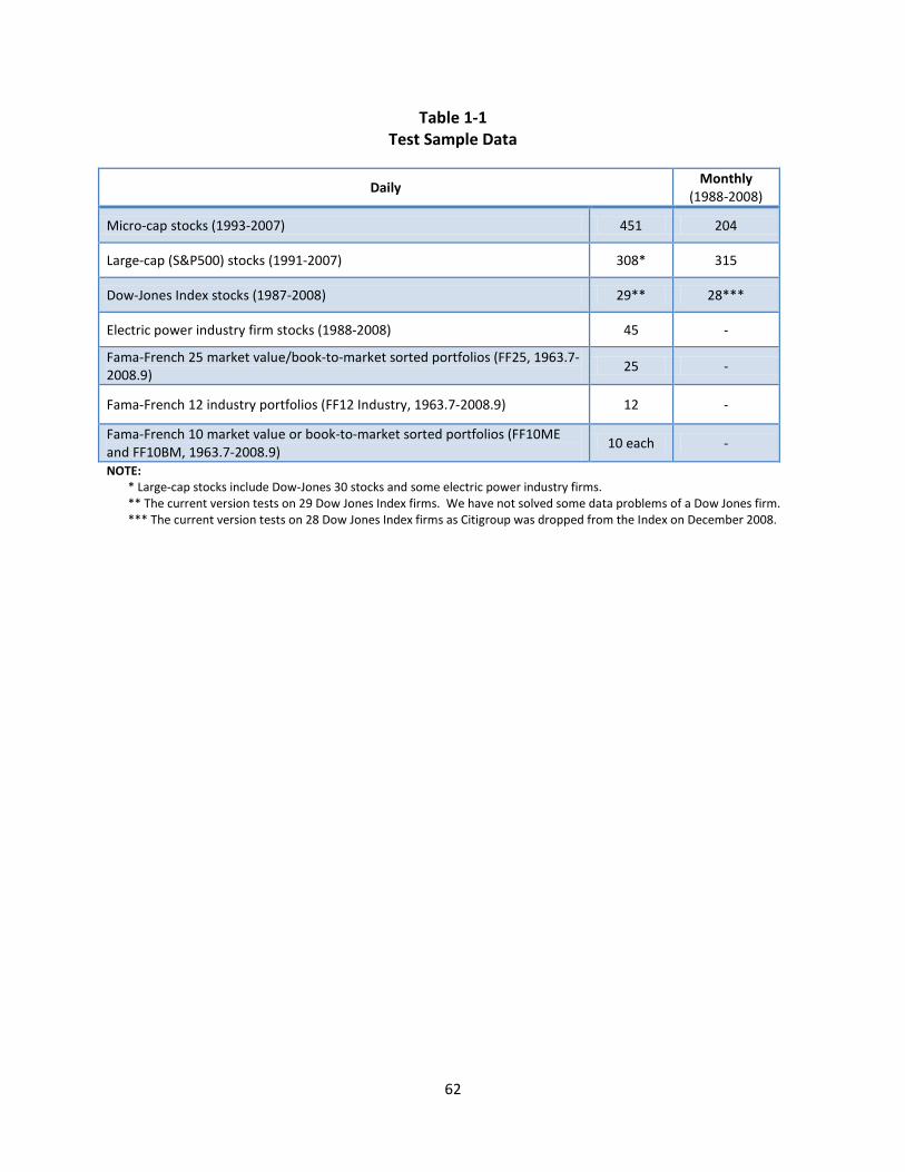
62

Table 1-1 Test Sample Data

Daily Monthly

(1988-2008)

Micro-cap stocks (1993-2007) 451 204

Large-cap (S&P500) stocks (1991-2007) 308* 315

Dow-Jones Index stocks (1987-2008) 29** 28***

Electric power industry firm stocks (1988-2008) 45 -

Fama-French 25 market value/book-to-market sorted portfolios (FF25, 1963.7-2008.9) 25 -

Fama-French 12 industry portfolios (FF12 Industry, 1963.7-2008.9) 12 -

Fama-French 10 market value or book-to-market sorted portfolios (FF10ME and FF10BM, 1963.7-2008.9) 10 each -

NOTE: * Large-cap stocks include Dow-Jones 30 stocks and some electric power industry firms. ** The current version tests on 29 Dow Jones Index firms. We have not solved some data problems of a Dow Jones firm. *** The current version tests on 28 Dow Jones Index firms as Citigroup was dropped from the Index on December 2008.

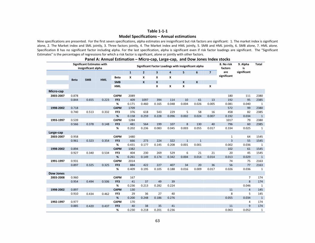
63

Table 1-1-1 Model Specifications – Annual estimations

Nine specifications are presented. For the first seven specifications, alpha estimates are insignificant but risk factors are significant: 1. The market index is significant alone, 2. The Market index and SML jointly, 3. Three factors jointly, 4. The Market index and HML jointly, 5. SMB and HML jointly, 6. SMB alone, 7. HML alone. Specification 8 has no significant factor including alpha. For the last specification, alpha is significant even if risk factor loadings are significant. The “Significant Estimates” is the percentages of regressions for which a risk factor is significant, alone or jointly with other factors.

Panel A: Annual Estimation – Micro-cap, Large-cap, and Dow Jones Index stocks

Significant Estimates with insignificant alpha

Significant Factor Loadings with insignificant alpha

8. No risk factors

are significant

9. Alpha is

significant

Total

Beta SMB HML

1 2 3 4 5 6 7

Beta X X X X

SMB X X X X HML X X X X

Micro-cap 2003-2007 0.878 CAPM 2089 180 111 2380

0.844 0.655 0.223 FF3 409 1097 394 114 10 61 13 192 95 2385 % 0.171 0.460 0.165 0.048 0.004 0.026 0.005 0.081 0.040 1

1998-2002 0.718 CAPM 1709 572 99 2380 0.740 0.513 0.332 FF3 376 618 543 229 5 58 16 458 82 2385 % 0.158 0.259 0.228 0.096 0.002 0.024 0.007 0.192 0.034 1

1993-1997 0.539 CAPM 1284 1017 79 2380 0.566 0.378 0.148 FF3 481 564 199 107 8 130 40 796 60 2385 % 0.202 0.236 0.083 0.045 0.003 0.055 0.017 0.334 0.025 1

Large-cap 2003-2007 0.958 CAPM 1480 1 64 1545

0.961 0.323 0.354 FF3 666 273 224 322 1 1 3 55 1545 % 0.431 0.177 0.145 0.208 0.001 0.001 0.002 0.036 1

1998-2002 0.894 CAPM 1382 102 61 1545 0.927 0.340 0.534 FF3 404 230 269 529 6 21 21 20 45 1545 % 0.261 0.149 0.174 0.342 0.004 0.014 0.014 0.013 0.029 1

1991-1997 0.931 CAPM 2014 74 75 2163 0.897 0.325 0.325 FF3 884 422 227 407 34 20 36 56 77 2163 % 0.409 0.195 0.105 0.188 0.016 0.009 0.017 0.026 0.036 1 Dow Jones

2003-2008 0.960 CAPM 167 7 174 0.954 0.494 0.506 FF3 41 37 49 39 8 174 % 0.236 0.213 0.282 0.224 0.046 1

1998-2002 0.897 CAPM 130 11 4 145 0.910 0.434 0.462 FF3 29 36 27 40 8 5 145

% 0.200 0.248 0.186 0.276 0.055 0.034 1

1992-1997 0.977

CAPM 170 4 174 0.885 0.420 0.437 FF3 40 38 35 41 11 9 174 % 0.230 0.218 0.201 0.236 0.063 0.052 1

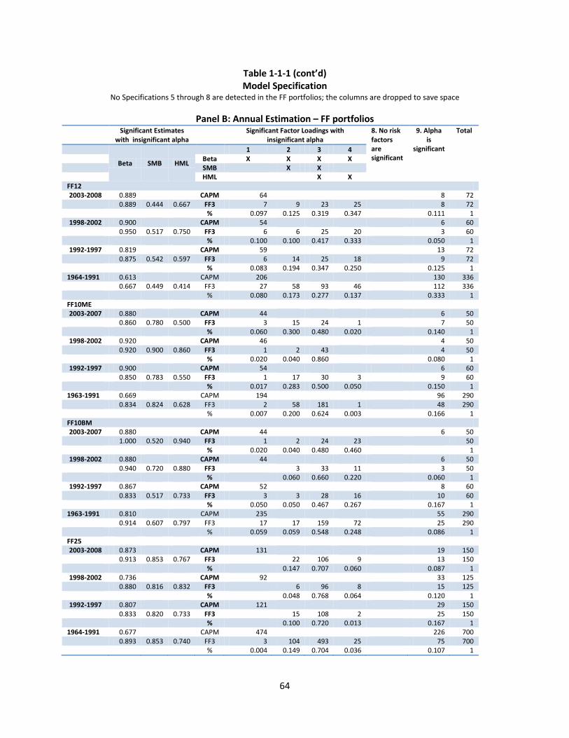
64

Table 1-1-1 (cont’d) Model Specification

No Specifications 5 through 8 are detected in the FF portfolios; the columns are dropped to save space

Panel B: Annual Estimation – FF portfolios Significant Estimates

with insignificant alpha Significant Factor Loadings with

insignificant alpha 8. No risk factors are significant

9. Alpha is

significant

Total

Beta SMB HML

1 2 3 4 Beta X X X X SMB X X HML X X FF12 2003-2008 0.889 CAPM 64 8 72

0.889 0.444 0.667 FF3 7 9 23 25 8 72 % 0.097 0.125 0.319 0.347 0.111 1

1998-2002 0.900 CAPM 54 6 60 0.950 0.517 0.750 FF3 6 6 25 20 3 60 % 0.100 0.100 0.417 0.333 0.050 1

1992-1997 0.819 CAPM 59 13 72 0.875 0.542 0.597 FF3 6 14 25 18 9 72 % 0.083 0.194 0.347 0.250 0.125 1 1964-1991 0.613 CAPM 206 130 336 0.667 0.449 0.414 FF3 27 58 93 46 112 336 % 0.080 0.173 0.277 0.137 0.333 1 FF10ME 2003-2007 0.880 CAPM 44 6 50

0.860 0.780 0.500 FF3 3 15 24 1 7 50 % 0.060 0.300 0.480 0.020 0.140 1

1998-2002 0.920 CAPM 46 4 50 0.920 0.900 0.860 FF3 1 2 43 4 50 % 0.020 0.040 0.860 0.080 1

1992-1997 0.900 CAPM 54 6 60 0.850 0.783 0.550 FF3 1 17 30 3 9 60 % 0.017 0.283 0.500 0.050 0.150 1 1963-1991 0.669 CAPM 194 96 290 0.834 0.824 0.628 FF3 2 58 181 1 48 290 % 0.007 0.200 0.624 0.003 0.166 1 FF10BM 2003-2007 0.880 CAPM 44 6 50

1.000 0.520 0.940 FF3 1 2 24 23 50 % 0.020 0.040 0.480 0.460 1

1998-2002 0.880 CAPM 44 6 50 0.940 0.720 0.880 FF3 3 33 11 3 50 % 0.060 0.660 0.220 0.060 1

1992-1997 0.867 CAPM 52 8 60 0.833 0.517 0.733 FF3 3 3 28 16 10 60 % 0.050 0.050 0.467 0.267 0.167 1 1963-1991 0.810 CAPM 235 55 290 0.914 0.607 0.797 FF3 17 17 159 72 25 290 % 0.059 0.059 0.548 0.248 0.086 1 FF25 2003-2008 0.873 CAPM 131 19 150

0.913 0.853 0.767 FF3 22 106 9 13 150 % 0.147 0.707 0.060 0.087 1 1998-2002 0.736 CAPM 92 33 125

0.880 0.816 0.832 FF3 6 96 8 15 125 % 0.048 0.768 0.064 0.120 1

1992-1997 0.807 CAPM 121 29 150 0.833 0.820 0.733 FF3 15 108 2 25 150 % 0.100 0.720 0.013 0.167 1 1964-1991 0.677 CAPM 474 226 700 0.893 0.853 0.740 FF3 3 104 493 25 75 700 % 0.004 0.149 0.704 0.036 0.107 1

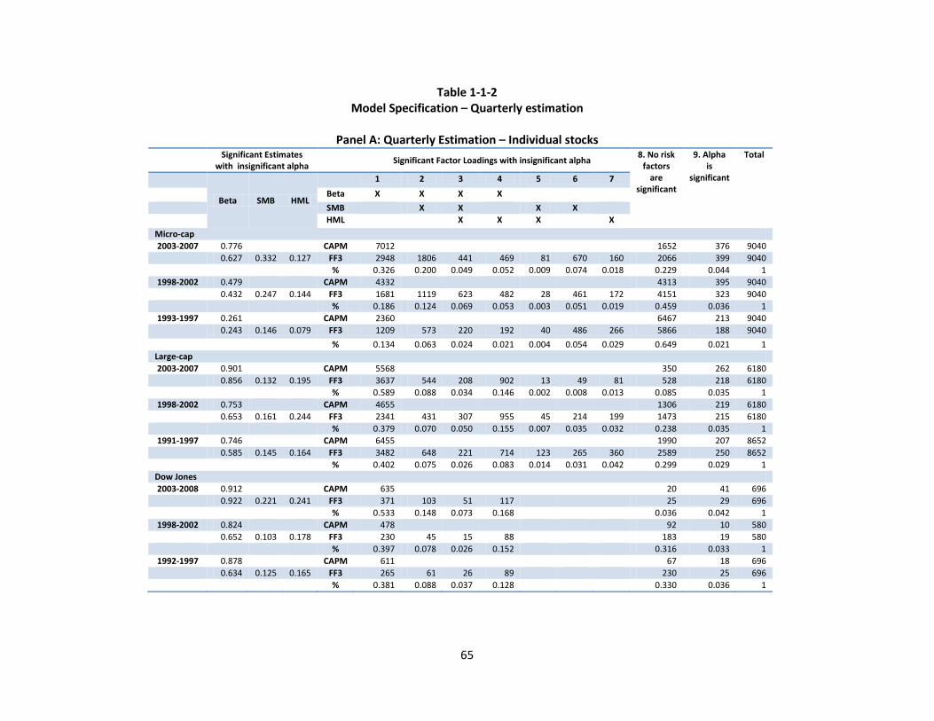
65

Table 1-1-2 Model Specification – Quarterly estimation

Panel A: Quarterly Estimation – Individual stocks

Significant Estimates with insignificant alpha

Significant Factor Loadings with insignificant alpha

8. No risk factors

are significant

9. Alpha is

significant

Total

Beta SMB HML

1 2 3 4 5 6 7

Beta X X X X

SMB X X X X HML X X X X

Micro-cap 2003-2007 0.776 CAPM 7012 1652 376 9040

0.627 0.332 0.127 FF3 2948 1806 441 469 81 670 160 2066 399 9040 % 0.326 0.200 0.049 0.052 0.009 0.074 0.018 0.229 0.044 1

1998-2002 0.479 CAPM 4332 4313 395 9040 0.432 0.247 0.144 FF3 1681 1119 623 482 28 461 172 4151 323 9040 % 0.186 0.124 0.069 0.053 0.003 0.051 0.019 0.459 0.036 1

1993-1997 0.261 CAPM 2360 6467 213 9040 0.243 0.146 0.079 FF3 1209 573 220 192 40 486 266 5866 188 9040

% 0.134 0.063 0.024 0.021 0.004 0.054 0.029 0.649 0.021 1 Large-cap 2003-2007 0.901 CAPM 5568 350 262 6180

0.856 0.132 0.195 FF3 3637 544 208 902 13 49 81 528 218 6180 % 0.589 0.088 0.034 0.146 0.002 0.008 0.013 0.085 0.035 1 1998-2002 0.753 CAPM 4655 1306 219 6180

0.653 0.161 0.244 FF3 2341 431 307 955 45 214 199 1473 215 6180 % 0.379 0.070 0.050 0.155 0.007 0.035 0.032 0.238 0.035 1

1991-1997 0.746 CAPM 6455 1990 207 8652 0.585 0.145 0.164 FF3 3482 648 221 714 123 265 360 2589 250 8652 % 0.402 0.075 0.026 0.083 0.014 0.031 0.042 0.299 0.029 1 Dow Jones 2003-2008 0.912 CAPM 635 20 41 696

0.922 0.221 0.241 FF3 371 103 51 117 25 29 696 % 0.533 0.148 0.073 0.168 0.036 0.042 1 1998-2002 0.824 CAPM 478 92 10 580

0.652 0.103 0.178 FF3 230 45 15 88 183 19 580 % 0.397 0.078 0.026 0.152 0.316 0.033 1

1992-1997 0.878 CAPM 611 67 18 696 0.634 0.125 0.165 FF3 265 61 26 89 230 25 696 % 0.381 0.088 0.037 0.128 0.330 0.036 1

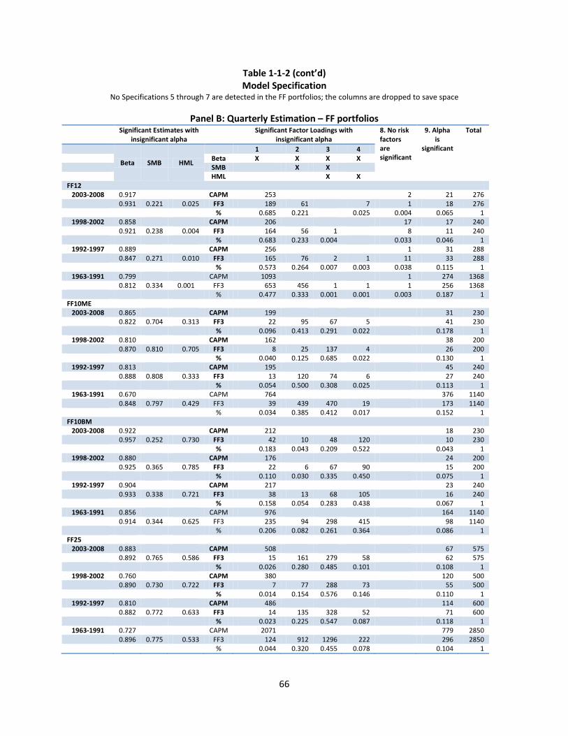
66

Table 1-1-2 (cont’d) Model Specification

No Specifications 5 through 7 are detected in the FF portfolios; the columns are dropped to save space

Panel B: Quarterly Estimation – FF portfolios Significant Estimates with

insignificant alpha Significant Factor Loadings with

insignificant alpha 8. No risk factors are significant

9. Alpha is

significant

Total

Beta SMB HML

1 2 3 4 Beta X X X X SMB X X HML X X FF12

2003-2008 0.917 CAPM 253 2 21 276 0.931 0.221 0.025 FF3 189 61 7 1 18 276 % 0.685 0.221 0.025 0.004 0.065 1

1998-2002 0.858 CAPM 206 17 17 240 0.921 0.238 0.004 FF3 164 56 1 8 11 240 % 0.683 0.233 0.004 0.033 0.046 1

1992-1997 0.889 CAPM 256 1 31 288 0.847 0.271 0.010 FF3 165 76 2 1 11 33 288 % 0.573 0.264 0.007 0.003 0.038 0.115 1

1963-1991 0.799 CAPM 1093 1 274 1368 0.812 0.334 0.001 FF3 653 456 1 1 1 256 1368 % 0.477 0.333 0.001 0.001 0.003 0.187 1 FF10ME

2003-2008 0.865 CAPM 199 31 230 0.822 0.704 0.313 FF3 22 95 67 5 41 230 % 0.096 0.413 0.291 0.022 0.178 1

1998-2002 0.810 CAPM 162 38 200 0.870 0.810 0.705 FF3 8 25 137 4 26 200 % 0.040 0.125 0.685 0.022 0.130 1

1992-1997 0.813 CAPM 195 45 240 0.888 0.808 0.333 FF3 13 120 74 6 27 240 % 0.054 0.500 0.308 0.025 0.113 1

1963-1991 0.670 CAPM 764 376 1140 0.848 0.797 0.429 FF3 39 439 470 19 173 1140 % 0.034 0.385 0.412 0.017 0.152 1 FF10BM

2003-2008 0.922 CAPM 212 18 230 0.957 0.252 0.730 FF3 42 10 48 120 10 230 % 0.183 0.043 0.209 0.522 0.043 1

1998-2002 0.880 CAPM 176 24 200 0.925 0.365 0.785 FF3 22 6 67 90 15 200 % 0.110 0.030 0.335 0.450 0.075 1

1992-1997 0.904 CAPM 217 23 240 0.933 0.338 0.721 FF3 38 13 68 105 16 240 % 0.158 0.054 0.283 0.438 0.067 1

1963-1991 0.856 CAPM 976 164 1140 0.914 0.344 0.625 FF3 235 94 298 415 98 1140 % 0.206 0.082 0.261 0.364 0.086 1 FF25

2003-2008 0.883 CAPM 508 67 575 0.892 0.765 0.586 FF3 15 161 279 58 62 575 % 0.026 0.280 0.485 0.101 0.108 1

1998-2002 0.760 CAPM 380 120 500 0.890 0.730 0.722 FF3 7 77 288 73 55 500 % 0.014 0.154 0.576 0.146 0.110 1

1992-1997 0.810 CAPM 486 114 600 0.882 0.772 0.633 FF3 14 135 328 52 71 600 % 0.023 0.225 0.547 0.087 0.118 1

1963-1991 0.727 CAPM 2071 779 2850 0.896 0.775 0.533 FF3 124 912 1296 222 296 2850 % 0.044 0.320 0.455 0.078 0.104 1

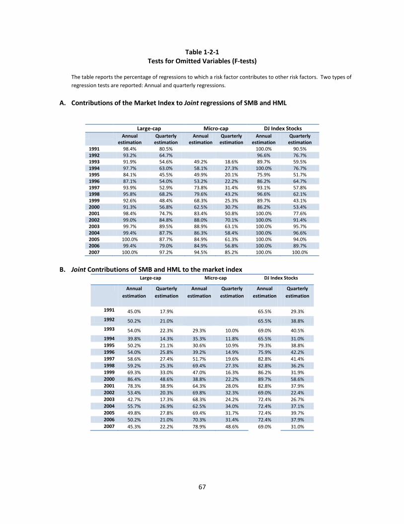
67

Table 1-2-1 Tests for Omitted Variables (F-tests)

The table reports the percentage of regressions to which a risk factor contributes to other risk factors. Two types of regression tests are reported: Annual and quarterly regressions.

A. Contributions of the Market Index to Joint regressions of SMB and HML

Large-cap Micro-cap DJ Index Stocks Annual

estimation Quarterly

estimation Annual

estimation Quarterly estimation

Annual estimation

Quarterly estimation

1991 98.4% 80.5%

100.0% 90.5% 1992 93.2% 64.7%

96.6% 76.7%

1993 91.9% 54.6% 49.2% 18.6% 89.7% 59.5% 1994 97.7% 63.0% 58.1% 27.3% 100.0% 76.7% 1995 84.1% 45.5% 49.9% 20.1% 75.9% 51.7% 1996 87.1% 54.0% 53.2% 22.2% 86.2% 64.7% 1997 93.9% 52.9% 73.8% 31.4% 93.1% 57.8% 1998 95.8% 68.2% 79.6% 43.2% 96.6% 62.1% 1999 92.6% 48.4% 68.3% 25.3% 89.7% 43.1% 2000 91.3% 56.8% 62.5% 30.7% 86.2% 53.4% 2001 98.4% 74.7% 83.4% 50.8% 100.0% 77.6% 2002 99.0% 84.8% 88.0% 70.1% 100.0% 91.4% 2003 99.7% 89.5% 88.9% 63.1% 100.0% 95.7% 2004 99.4% 87.7% 86.3% 58.4% 100.0% 96.6% 2005 100.0% 87.7% 84.9% 61.3% 100.0% 94.0% 2006 99.4% 79.0% 84.9% 56.8% 100.0% 89.7% 2007 100.0% 97.2% 94.5% 85.2% 100.0% 100.0%

B. Joint Contributions of SMB and HML to the market index

Large-cap Micro-cap DJ Index Stocks

Annual estimation

Quarterly estimation

Annual estimation

Quarterly estimation

Annual estimation

Quarterly estimation

1991 45.0% 17.9%

65.5% 29.3%

1992 50.2% 21.0%

65.5% 38.8%

1993 54.0% 22.3% 29.3% 10.0% 69.0% 40.5%

1994 39.8% 14.3% 35.3% 11.8% 65.5% 31.0% 1995 50.2% 21.1% 30.6% 10.9% 79.3% 38.8% 1996 54.0% 25.8% 39.2% 14.9% 75.9% 42.2% 1997 58.6% 27.4% 51.7% 19.6% 82.8% 41.4% 1998 59.2% 25.3% 69.4% 27.3% 82.8% 36.2% 1999 69.3% 33.0% 47.0% 16.3% 86.2% 31.9% 2000 86.4% 48.6% 38.8% 22.2% 89.7% 58.6% 2001 78.3% 38.9% 64.3% 28.0% 82.8% 37.9% 2002 53.4% 20.3% 69.8% 32.3% 69.0% 22.4% 2003 42.7% 17.3% 68.3% 24.2% 72.4% 26.7% 2004 55.7% 26.9% 62.5% 34.0% 72.4% 37.1% 2005 49.8% 27.8% 69.4% 31.7% 72.4% 39.7% 2006 50.2% 21.0% 70.3% 31.4% 72.4% 37.9% 2007 45.3% 22.2% 78.9% 48.6% 69.0% 31.0%

68

Table 1-2-1 (cont’d)

Tests for Omitted variables (F-tests)

Fama-French Portfolios

For the FF25 portfolios: The market index makes contribution to all 25 portfolios on an annual basis throughout the entire period. So do SMB and HML, except for a few years for a few portfolios in the 1970s. On a quarterly basis, the market index also makes contribution to all 25 portfolios. But SMB and HML jointly make contribution to all portfolios except six large capitalization portfolios: s4h2 (84%), s4h3 (86%), s4h4 (87%), s4h5 (87%), s5h2 (69%), and s5h3 (78%). The failures to make contribution are inter-temporally dispersed and show no clear temporal patterns. For the FF10ME and FF10BM portfolios: The market index also makes contribution to all portfolios throughout the entire period. The table below reports individual contributions of SMB and HML to the market index for FF10ME and FF10BM. The pattern is consistent with the findings in the model specification test. SMB makes more contribution to the FF10ME than HML does. HML makes more contribution to the FF10BM than SMB does.

FF10ME FF10BM Count of

contributions to the market index

Percent Count of

contributions to the market index

Percent

SMB HML SMB HML SMB HML SMB HML d1 46 27 1.000 0.587 21 45 0.457 0.978 d2 46 27 1.000 0.587 19 39 0.413 0.848 d3 46 31 1.000 0.674 19 30 0.413 0.652 d4 46 29 1.000 0.630 27 33 0.587 0.717 d5 46 31 1.000 0.674 24 38 0.522 0.826 d6 46 28 1.000 0.609 27 40 0.587 0.870 d7 46 28 1.000 0.609 28 45 0.609 0.978 d8 46 30 1.000 0.652 25 46 0.543 1.000 d9 25 33 0.543 0.717 27 46 0.587 1.000 d10 46 30 1.000 0.652 27 46 0.587 1.000 Average 0.954 0.639 0.530 0.887

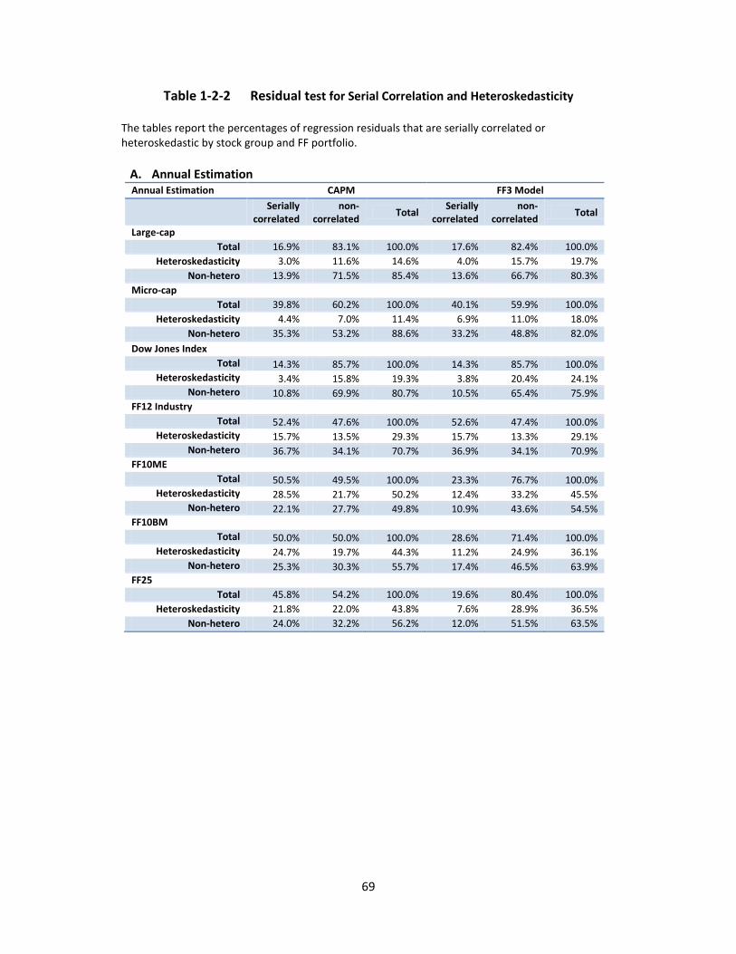
69

Table 1-2-2 Residual test for Serial Correlation and Heteroskedasticity

The tables report the percentages of regression residuals that are serially correlated or heteroskedastic by stock group and FF portfolio.

A. Annual Estimation Annual Estimation CAPM FF3 Model

Serially correlated

non-correlated

Total Serially

correlated non-

correlated Total

Large-cap Total 16.9% 83.1% 100.0% 17.6% 82.4% 100.0%

Heteroskedasticity 3.0% 11.6% 14.6% 4.0% 15.7% 19.7% Non-hetero 13.9% 71.5% 85.4% 13.6% 66.7% 80.3%

Micro-cap Total 39.8% 60.2% 100.0% 40.1% 59.9% 100.0%

Heteroskedasticity 4.4% 7.0% 11.4% 6.9% 11.0% 18.0% Non-hetero 35.3% 53.2% 88.6% 33.2% 48.8% 82.0%

Dow Jones Index Total 14.3% 85.7% 100.0% 14.3% 85.7% 100.0%

Heteroskedasticity 3.4% 15.8% 19.3% 3.8% 20.4% 24.1% Non-hetero 10.8% 69.9% 80.7% 10.5% 65.4% 75.9%

FF12 Industry Total 52.4% 47.6% 100.0% 52.6% 47.4% 100.0%

Heteroskedasticity 15.7% 13.5% 29.3% 15.7% 13.3% 29.1% Non-hetero 36.7% 34.1% 70.7% 36.9% 34.1% 70.9%

FF10ME Total 50.5% 49.5% 100.0% 23.3% 76.7% 100.0%

Heteroskedasticity 28.5% 21.7% 50.2% 12.4% 33.2% 45.5% Non-hetero 22.1% 27.7% 49.8% 10.9% 43.6% 54.5%

FF10BM Total 50.0% 50.0% 100.0% 28.6% 71.4% 100.0%

Heteroskedasticity 24.7% 19.7% 44.3% 11.2% 24.9% 36.1% Non-hetero 25.3% 30.3% 55.7% 17.4% 46.5% 63.9%

FF25 Total 45.8% 54.2% 100.0% 19.6% 80.4% 100.0%

Heteroskedasticity 21.8% 22.0% 43.8% 7.6% 28.9% 36.5% Non-hetero 24.0% 32.2% 56.2% 12.0% 51.5% 63.5%

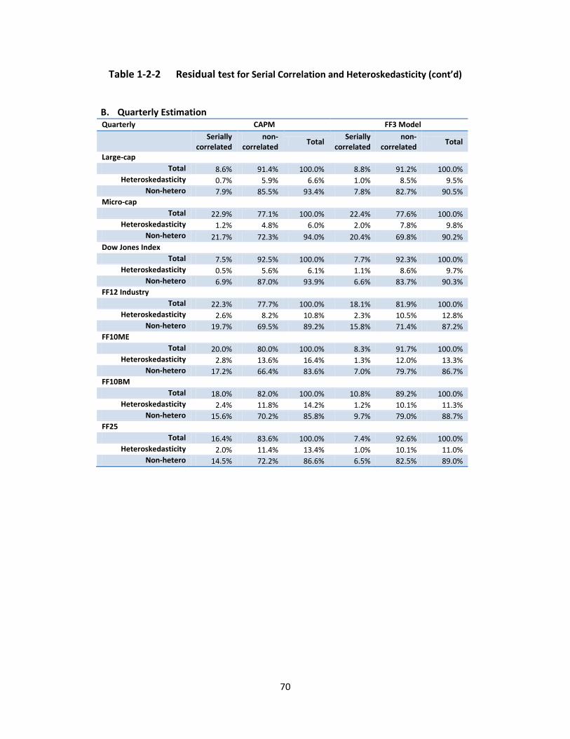
70

Table 1-2-2 Residual test for Serial Correlation and Heteroskedasticity (cont’d)

B. Quarterly Estimation Quarterly CAPM FF3 Model

Serially correlated

non-correlated

Total Serially

correlated non-

correlated Total

Large-cap Total 8.6% 91.4% 100.0% 8.8% 91.2% 100.0%

Heteroskedasticity 0.7% 5.9% 6.6% 1.0% 8.5% 9.5% Non-hetero 7.9% 85.5% 93.4% 7.8% 82.7% 90.5%

Micro-cap Total 22.9% 77.1% 100.0% 22.4% 77.6% 100.0%

Heteroskedasticity 1.2% 4.8% 6.0% 2.0% 7.8% 9.8% Non-hetero 21.7% 72.3% 94.0% 20.4% 69.8% 90.2%

Dow Jones Index Total 7.5% 92.5% 100.0% 7.7% 92.3% 100.0%

Heteroskedasticity 0.5% 5.6% 6.1% 1.1% 8.6% 9.7% Non-hetero 6.9% 87.0% 93.9% 6.6% 83.7% 90.3%

FF12 Industry Total 22.3% 77.7% 100.0% 18.1% 81.9% 100.0%

Heteroskedasticity 2.6% 8.2% 10.8% 2.3% 10.5% 12.8% Non-hetero 19.7% 69.5% 89.2% 15.8% 71.4% 87.2%

FF10ME Total 20.0% 80.0% 100.0% 8.3% 91.7% 100.0%

Heteroskedasticity 2.8% 13.6% 16.4% 1.3% 12.0% 13.3% Non-hetero 17.2% 66.4% 83.6% 7.0% 79.7% 86.7%

FF10BM Total 18.0% 82.0% 100.0% 10.8% 89.2% 100.0%

Heteroskedasticity 2.4% 11.8% 14.2% 1.2% 10.1% 11.3% Non-hetero 15.6% 70.2% 85.8% 9.7% 79.0% 88.7%

FF25 Total 16.4% 83.6% 100.0% 7.4% 92.6% 100.0%

Heteroskedasticity 2.0% 11.4% 13.4% 1.0% 10.1% 11.0% Non-hetero 14.5% 72.2% 86.6% 6.5% 82.5% 89.0%

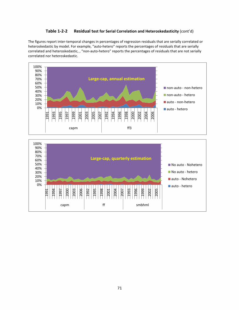
71

Table 1-2-2 Residual test for Serial Correlation and Heteroskedasticity (cont’d) The figures report inter-temporal changes in percentages of regression residuals that are serially correlated or heteroskedastic by model. For example, “auto-hetero” reports the percentages of residuals that are serially correlated and heteroskedastic, , “non-auto-hetero” reports the percentages of residuals that are not serially correlated nor heteroskedastic.

0%10%20%30%40%50%60%70%80%90%

100%

1991

1993

1995

1997

1999

2001

2003

2005

2007

1992

1994

1996

1998

2000

2002

2004

2006

capm ff3

Large-cap, annual estimation

non-auto - non-hetero

non-auto - hetero

auto - non-hetero

auto - hetero

0%10%20%30%40%50%60%70%80%90%

100%

1991

1994

1997

2000

2003

2006

1992

1995

1998

2001

2004

2007

1993

1996

1999

2002

2005

capm ff smbhml

Large-cap, quarterly estimationNo auto - Nohetero

No auto - hetero

auto - Nohetero

auto - hetero

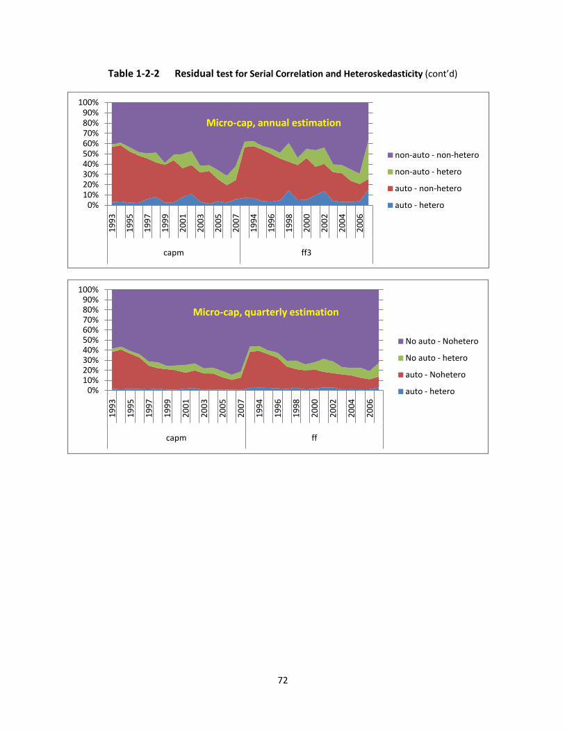
72

Table 1-2-2 Residual test for Serial Correlation and Heteroskedasticity (cont’d)

0%10%20%30%40%50%60%70%80%90%

100%19

93

1995

1997

1999

2001

2003

2005

2007

1994

1996

1998

2000

2002

2004

2006

capm ff3

Micro-cap, annual estimation

non-auto - non-hetero

non-auto - hetero

auto - non-hetero

auto - hetero

0%10%20%30%40%50%60%70%80%90%

100%

1993

1995

1997

1999

2001

2003

2005

2007

1994

1996

1998

2000

2002

2004

2006

capm ff

Micro-cap, quarterly estimation

No auto - Nohetero

No auto - hetero

auto - Nohetero

auto - hetero

73

Table 1-2-2 Residual test for Serial Correlation and Heteroskedasticity (cont’d)

0%10%20%30%40%50%60%70%80%90%

100%19

8719

8919

9119

9319

9519

9719

9920

0120

0320

0520

0719

8719

8919

9119

9319

9519

9719

9920

0120

0320

0520

07

capm ff

Dow Jones Stocks, Annual estimation

No auto - Nohetero

No auto - hetero

auto - Nohetero

auto - hetero

0%10%20%30%40%50%60%70%80%90%

100%

1987

1989

1991

1993

1995

1997

1999

2001

2003

2005

2007

1987

1989

1991

1993

1995

1997

1999

2001

2003

2005

2007

capm ff

Dow Jones Stocks, Quarterly estimation

No auto - Nohetero

No auto - hetero

auto - Nohetero

auto - hetero

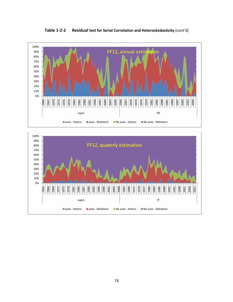
74

Table 1-2-2 Residual test for Serial Correlation and Heteroskedasticity (cont’d)

0%

10%

20%

30%

40%

50%

60%

70%

80%

90%

100%19

64

1967

1970

1973

1976

1979

1982

1985

1988

1991

1994

1997

2000

2003

2006

1964

1967

1970

1973

1976

1979

1982

1985

1988

1991

1994

1997

2000

2003

2006

capm ff3

FF12, annual estimation

auto - hetero auto - Nohetero No auto - hetero No auto - Nohetero

0%

10%

20%

30%

40%

50%

60%

70%

80%

90%

100%

1963

1966

1969

1972

1975

1978

1981

1984

1987

1990

1993

1996

1999

2002

2005

2008

1965

1968

1971

1974

1977

1980

1983

1986

1989

1992

1995

1998

2001

2004

2007

capm ff

FF12, quaterly estimation

auto - hetero auto - Nohetero No auto - hetero No auto - Nohetero

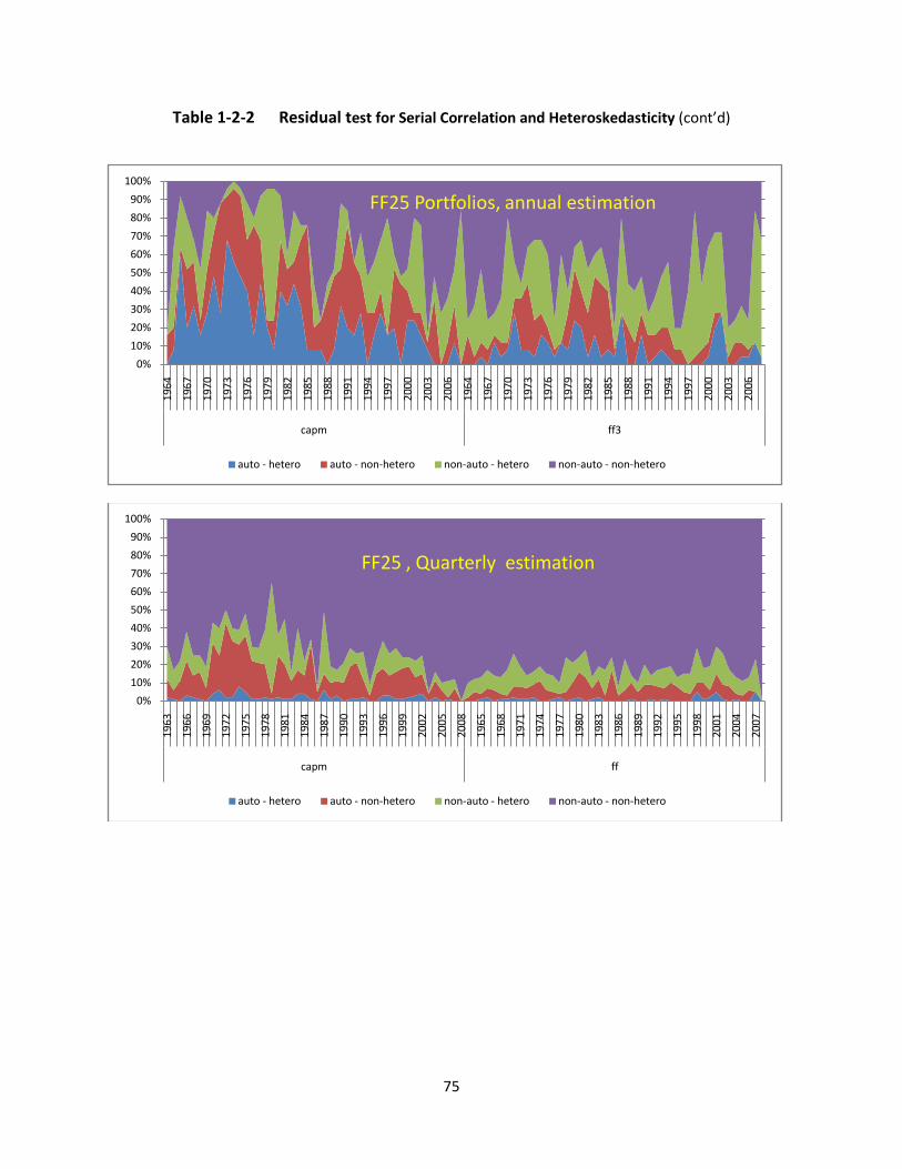
75

Table 1-2-2 Residual test for Serial Correlation and Heteroskedasticity (cont’d)

0%

10%

20%

30%

40%

50%

60%

70%

80%

90%

100%19

64

1967

1970

1973

1976

1979

1982

1985

1988

1991

1994

1997

2000

2003

2006

1964

1967

1970

1973

1976

1979

1982

1985

1988

1991

1994

1997

2000

2003

2006

capm ff3

FF25 Portfolios, annual estimation

auto - hetero auto - non-hetero non-auto - hetero non-auto - non-hetero

0%

10%

20%

30%

40%

50%

60%

70%

80%

90%

100%

1963

1966

1969

1972

1975

1978

1981

1984

1987

1990

1993

1996

1999

2002

2005

2008

1965

1968

1971

1974

1977

1980

1983

1986

1989

1992

1995

1998

2001

2004

2007

capm ff

FF25 , Quarterly estimation

auto - hetero auto - non-hetero non-auto - hetero non-auto - non-hetero

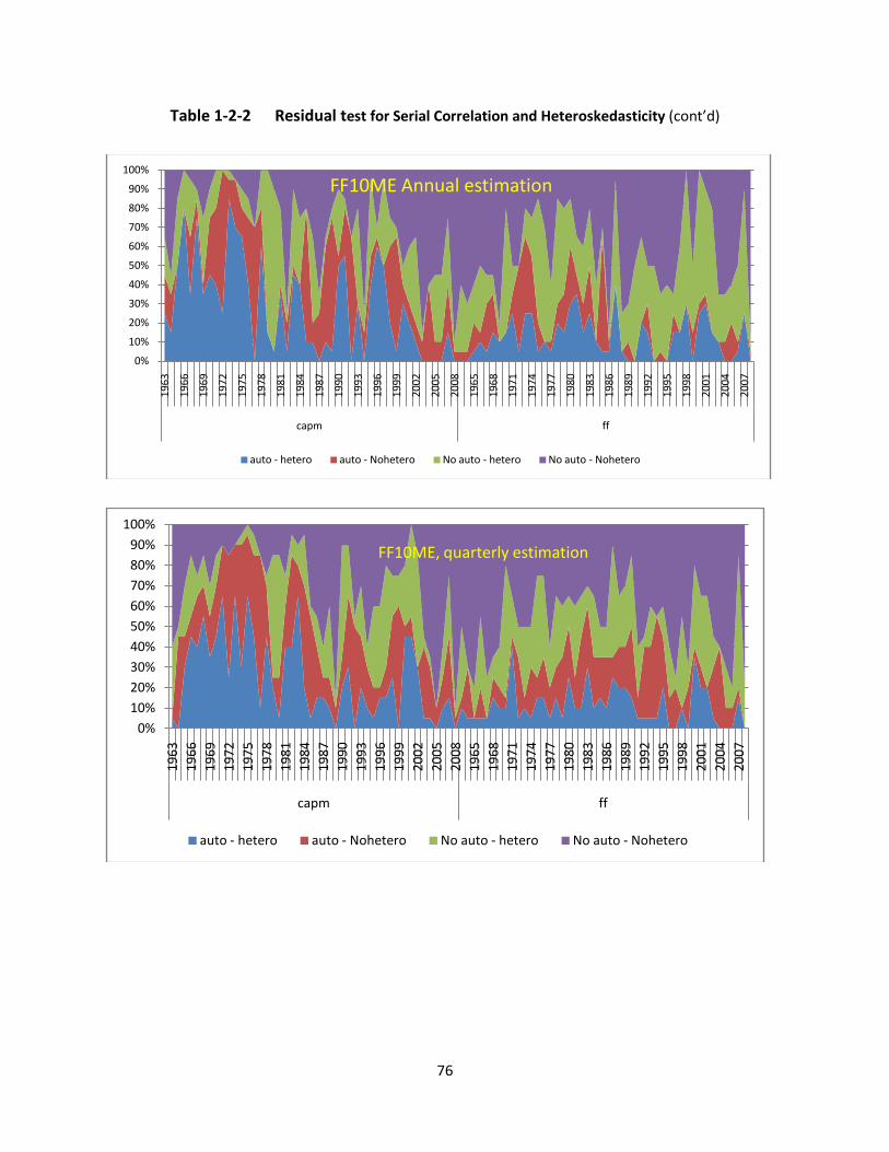
76

Table 1-2-2 Residual test for Serial Correlation and Heteroskedasticity (cont’d)

0%

10%

20%

30%

40%

50%

60%

70%

80%

90%

100%19

63

1966

1969

1972

1975

1978

1981

1984

1987

1990

1993

1996

1999

2002

2005

2008

1965

1968

1971

1974

1977

1980

1983

1986

1989

1992

1995

1998

2001

2004

2007

capm ff

FF10ME Annual estimation

auto - hetero auto - Nohetero No auto - hetero No auto - Nohetero

0%10%20%30%40%50%60%70%80%90%

100%

1963

1966

1969

1972

1975

1978

1981

1984

1987

1990

1993

1996

1999

2002

2005

2008

1965

1968

1971

1974

1977

1980

1983

1986

1989

1992

1995

1998

2001

2004

2007

capm ff

FF10ME, quarterly estimation

auto - hetero auto - Nohetero No auto - hetero No auto - Nohetero

77

Table 1-3 R2, Factor Loading Estimates, and Variability

All numbers represent the statistics of the regressions with significant market beta and insignificant alpha for each subsample period. The count of firms is a total number of regressions with significant market beta and insignificant alpha for each subsample period. Therefore, quarterly regressions have larger numbers of count.

Panel A: Individual Stocks

Micro-cap stocks Large-cap stocks Dow Jones Index stocks Annual Quarterly Annual Quarterly Annual Quarterly CAPM FF CAPM FF CAPM FF CAPM FF CAPM FF CAPM FF Count of Firms

*1992-1997 1284 1351 2360 2194 2014 1940 6455 5065 170 154 611 441 1998-2002 1709 1766 4332 3905 1382 1432 4655 4034 130 132 478 378 2003-2007* 2089 2014 7012 5664 1480 1485 5568 5291 167 166 635 642

Average of adj_R2 *1992-1997 0.063 0.080 0.118 0.136 0.159 0.179 0.198 0.234 0.222 0.269 0.244 0.307 1998-2002 0.126 0.158 0.179 0.224 0.232 0.266 0.270 0.316 0.309 0.348 0.335 0.390 2003-2007* 0.222 0.272 0.258 0.328 0.285 0.312 0.303 0.338 0.391 0.424 0.382 0.419

Average of SBC *1992-1997 -4.710 -4.766 -4.703 -4.775 -5.345 -5.351 -5.384 -5.376 -5.728 -5.766 -5.715 -5.727 1998-2002 -4.276 -4.340 -4.325 -4.409 -4.700 -4.738 -4.778 -4.797 -5.016 -5.039 -5.051 -5.033 2003-2007* -5.049 -5.105 -5.146 -5.191 -5.843 -5.841 -5.880 -5.855 -6.076 -6.126 -6.133 -6.116

Average of Beta *1992-1997 0.934 1.208 1.327 1.813 1.112 1.185 1.266 1.472 1.172 1.133 1.258 1.372 1998-2002 0.779 1.069 1.003 1.428 0.928 1.124 1.062 1.373 0.977 1.024 1.069 1.257 2003-2007* 1.277 1.087 1.419 1.280 1.045 1.039 1.092 1.113 0.968 1.007 0.970 1.025

Volatility of Beta *1992-1997 0.552 0.556 0.944 1.148 0.516 0.488 0.614 0.654 0.399 0.480 0.450 0.522 1998-2002 0.505 0.494 0.643 0.794 0.491 0.444 0.549 0.605 0.421 0.446 0.427 0.471 2003-2007* 0.505 0.390 0.609 0.528 0.390 0.340 0.450 0.411 0.306 0.271 0.347 0.334

Volatility of Alpha *1992-1997 0.00138 0.00133 0.00285 0.00283 0.00100 0.00096 0.00196 0.00192 0.00068 0.00071 0.00148 0.00142 1998-2002 0.00182 0.00167 0.00349 0.00337 0.00139 0.00134 0.00265 0.00259 0.00089 0.00097 0.00204 0.00205 2003-2007* 0.00117 0.00110 0.00222 0.00218 0.00083 0.00079 0.00161 0.00156 0.00075 0.00072 0.00152 0.00143

NOTE: The test for Micro-cap stocks begins 1993 and Large-stocks in 1991. The test period for Dow Jones Index stocks end in 2008.

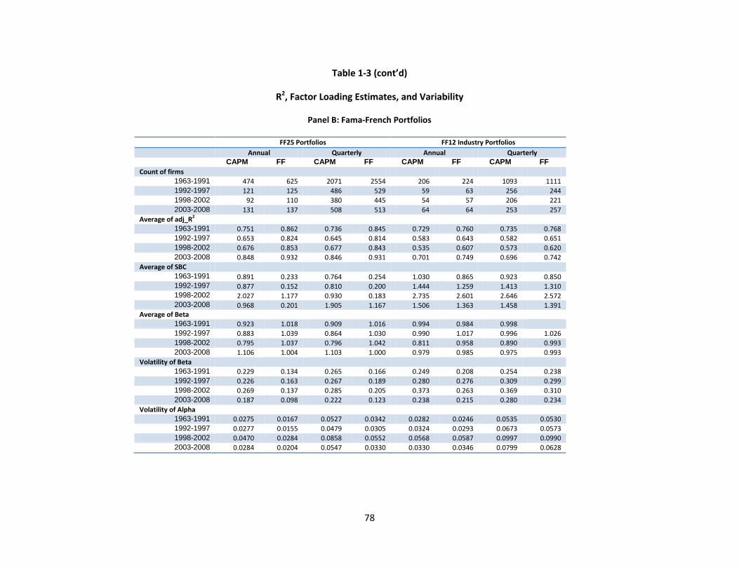
78

Table 1-3 (cont’d)

R2, Factor Loading Estimates, and Variability

Panel B: Fama-French Portfolios

FF25 Portfolios FF12 Industry Portfolios Annual Quarterly Annual Quarterly CAPM FF CAPM FF CAPM FF CAPM FF Count of firms

1963-1991 474 625 2071 2554 206 224 1093 1111 1992-1997 121 125 486 529 59 63 256 244 1998-2002 92 110 380 445 54 57 206 221 2003-2008 131 137 508 513 64 64 253 257

Average of adj_R2 1963-1991 0.751 0.862 0.736 0.845 0.729 0.760 0.735 0.768 1992-1997 0.653 0.824 0.645 0.814 0.583 0.643 0.582 0.651 1998-2002 0.676 0.853 0.677 0.843 0.535 0.607 0.573 0.620 2003-2008 0.848 0.932 0.846 0.931 0.701 0.749 0.696 0.742

Average of SBC 1963-1991 0.891 0.233 0.764 0.254 1.030 0.865 0.923 0.850 1992-1997 0.877 0.152 0.810 0.200 1.444 1.259 1.413 1.310 1998-2002 2.027 1.177 0.930 0.183 2.735 2.601 2.646 2.572 2003-2008 0.968 0.201 1.905 1.167 1.506 1.363 1.458 1.391

Average of Beta 1963-1991 0.923 1.018 0.909 1.016 0.994 0.984 0.998 1992-1997 0.883 1.039 0.864 1.030 0.990 1.017 0.996 1.026 1998-2002 0.795 1.037 0.796 1.042 0.811 0.958 0.890 0.993 2003-2008 1.106 1.004 1.103 1.000 0.979 0.985 0.975 0.993

Volatility of Beta 1963-1991 0.229 0.134 0.265 0.166 0.249 0.208 0.254 0.238 1992-1997 0.226 0.163 0.267 0.189 0.280 0.276 0.309 0.299 1998-2002 0.269 0.137 0.285 0.205 0.373 0.263 0.369 0.310 2003-2008 0.187 0.098 0.222 0.123 0.238 0.215 0.280 0.234

Volatility of Alpha 1963-1991 0.0275 0.0167 0.0527 0.0342 0.0282 0.0246 0.0535 0.0530 1992-1997 0.0277 0.0155 0.0479 0.0305 0.0324 0.0293 0.0673 0.0573 1998-2002 0.0470 0.0284 0.0858 0.0552 0.0568 0.0587 0.0997 0.0990 2003-2008 0.0284 0.0204 0.0547 0.0330 0.0330 0.0346 0.0799 0.0628

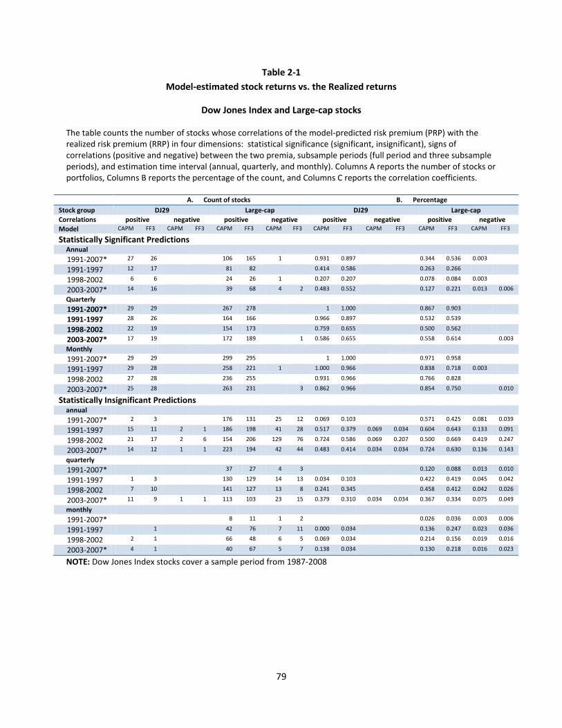
79

Table 2-1 Model-estimated stock returns vs. the Realized returns

Dow Jones Index and Large-cap stocks

The table counts the number of stocks whose correlations of the model-predicted risk premium (PRP) with the realized risk premium (RRP) in four dimensions: statistical significance (significant, insignificant), signs of correlations (positive and negative) between the two premia, subsample periods (full period and three subsample periods), and estimation time interval (annual, quarterly, and monthly). Columns A reports the number of stocks or portfolios, Columns B reports the percentage of the count, and Columns C reports the correlation coefficients.

A. Count of stocks B. Percentage Stock group DJ29 Large-cap DJ29 Large-cap Correlations positive negative positive negative positive negative positive negative Model CAPM FF3 CAPM FF3 CAPM FF3 CAPM FF3 CAPM FF3 CAPM FF3 CAPM FF3 CAPM FF3

Statistically Significant Predictions

Annual

1991-2007* 27 26 106 165 1 0.931 0.897 0.344 0.536 0.003

1991-1997 12 17 81 82 0.414 0.586 0.263 0.266

1998-2002 6 6 24 26 1 0.207 0.207 0.078 0.084 0.003

2003-2007* 14 16 39 68 4 2 0.483 0.552 0.127 0.221 0.013 0.006

Quarterly

1991-2007* 29 29 267 278 1 1.000 0.867 0.903

1991-1997 28 26 164 166 0.966 0.897 0.532 0.539

1998-2002 22 19 154 173 0.759 0.655 0.500 0.562

2003-2007* 17 19 172 189 1 0.586 0.655 0.558 0.614 0.003

Monthly

1991-2007* 29 29 299 295 1 1.000 0.971 0.958

1991-1997 29 28 258 221 1 1.000 0.966 0.838 0.718 0.003

1998-2002 27 28 236 255 0.931 0.966 0.766 0.828

2003-2007* 25 28 263 231 3 0.862 0.966 0.854 0.750 0.010

Statistically Insignificant Predictions

annual

1991-2007* 2 3 176 131 25 12 0.069 0.103 0.571 0.425 0.081 0.039

1991-1997 15 11 2 1 186 198 41 28 0.517 0.379 0.069 0.034 0.604 0.643 0.133 0.091

1998-2002 21 17 2 6 154 206 129 76 0.724 0.586 0.069 0.207 0.500 0.669 0.419 0.247

2003-2007* 14 12 1 1 223 194 42 44 0.483 0.414 0.034 0.034 0.724 0.630 0.136 0.143

quarterly

1991-2007* 37 27 4 3 0.120 0.088 0.013 0.010

1991-1997 1 3 130 129 14 13 0.034 0.103 0.422 0.419 0.045 0.042

1998-2002 7 10 141 127 13 8 0.241 0.345 0.458 0.412 0.042 0.026

2003-2007* 11 9 1 1 113 103 23 15 0.379 0.310 0.034 0.034 0.367 0.334 0.075 0.049

monthly

1991-2007* 8 11 1 2 0.026 0.036 0.003 0.006

1991-1997 1 42 76 7 11 0.000 0.034 0.136 0.247 0.023 0.036

1998-2002 2 1 66 48 6 5 0.069 0.034 0.214 0.156 0.019 0.016

2003-2007* 4 1 40 67 5 7 0.138 0.034 0.130 0.218 0.016 0.023

NOTE: Dow Jones Index stocks cover a sample period from 1987-2008

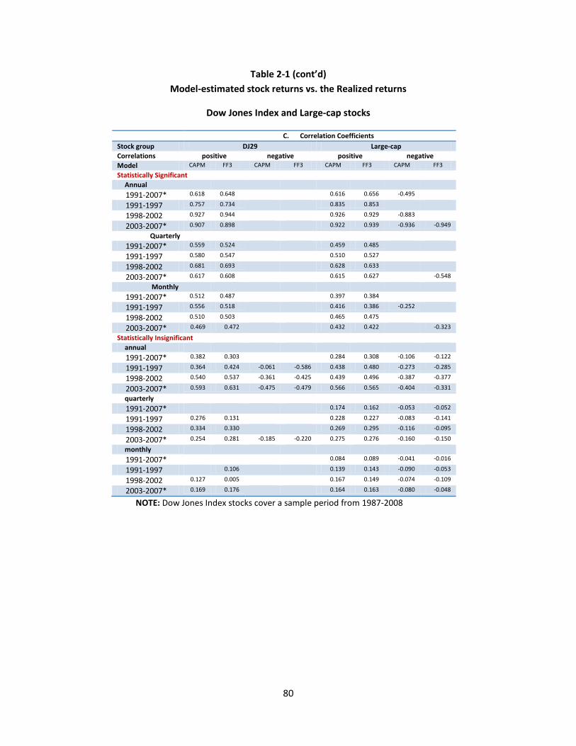
80

Table 2-1 (cont’d) Model-estimated stock returns vs. the Realized returns

Dow Jones Index and Large-cap stocks

C. Correlation Coefficients Stock group DJ29 Large-cap Correlations positive negative positive negative Model CAPM FF3 CAPM FF3 CAPM FF3 CAPM FF3

Statistically Significant

Annual

1991-2007* 0.618 0.648 0.616 0.656 -0.495

1991-1997 0.757 0.734 0.835 0.853

1998-2002 0.927 0.944 0.926 0.929 -0.883

2003-2007* 0.907 0.898 0.922 0.939 -0.936 -0.949

Quarterly

1991-2007* 0.559 0.524 0.459 0.485

1991-1997 0.580 0.547 0.510 0.527

1998-2002 0.681 0.693 0.628 0.633

2003-2007* 0.617 0.608 0.615 0.627 -0.548

Monthly

1991-2007* 0.512 0.487 0.397 0.384

1991-1997 0.556 0.518 0.416 0.386 -0.252

1998-2002 0.510 0.503 0.465 0.475

2003-2007* 0.469 0.472 0.432 0.422 -0.323

Statistically Insignificant

annual

1991-2007* 0.382 0.303 0.284 0.308 -0.106 -0.122

1991-1997 0.364 0.424 -0.061 -0.586 0.438 0.480 -0.273 -0.285

1998-2002 0.540 0.537 -0.361 -0.425 0.439 0.496 -0.387 -0.377

2003-2007* 0.593 0.631 -0.475 -0.479 0.566 0.565 -0.404 -0.331

quarterly

1991-2007* 0.174 0.162 -0.053 -0.052

1991-1997 0.276 0.131 0.228 0.227 -0.083 -0.141

1998-2002 0.334 0.330 0.269 0.295 -0.116 -0.095

2003-2007* 0.254 0.281 -0.185 -0.220 0.275 0.276 -0.160 -0.150

monthly

1991-2007* 0.084 0.089 -0.041 -0.016

1991-1997 0.106 0.139 0.143 -0.090 -0.053

1998-2002 0.127 0.005 0.167 0.149 -0.074 -0.109

2003-2007* 0.169 0.176 0.164 0.163 -0.080 -0.048

NOTE: Dow Jones Index stocks cover a sample period from 1987-2008

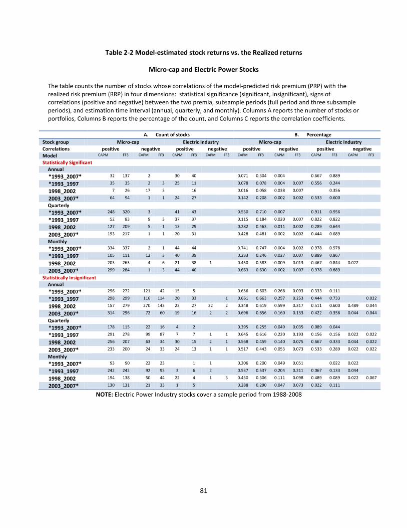
81

Table 2-2 Model-estimated stock returns vs. the Realized returns

Micro-cap and Electric Power Stocks

The table counts the number of stocks whose correlations of the model-predicted risk premium (PRP) with the realized risk premium (RRP) in four dimensions: statistical significance (significant, insignificant), signs of correlations (positive and negative) between the two premia, subsample periods (full period and three subsample periods), and estimation time interval (annual, quarterly, and monthly). Columns A reports the number of stocks or portfolios, Columns B reports the percentage of the count, and Columns C reports the correlation coefficients.

A. Count of stocks B. Percentage Stock group Micro-cap Electric Industry Micro-cap Electric Industry Correlations positive negative positive negative positive negative positive negative Model CAPM FF3 CAPM FF3 CAPM FF3 CAPM FF3 CAPM FF3 CAPM FF3 CAPM FF3 CAPM FF3

Statistically Significant

Annual

*1993_2007* 32 137 2 30 40 0.071 0.304 0.004 0.667 0.889

*1993_1997 35 35 2 3 25 11 0.078 0.078 0.004 0.007 0.556 0.244

1998_2002 7 26 17 3 16 0.016 0.058 0.038 0.007 0.356

2003_2007* 64 94 1 1 24 27 0.142 0.208 0.002 0.002 0.533 0.600

Quarterly

*1993_2007* 248 320 3 41 43 0.550 0.710 0.007 0.911 0.956

*1993_1997 52 83 9 3 37 37 0.115 0.184 0.020 0.007 0.822 0.822

1998_2002 127 209 5 1 13 29 0.282 0.463 0.011 0.002 0.289 0.644

2003_2007* 193 217 1 1 20 31 0.428 0.481 0.002 0.002 0.444 0.689

Monthly

*1993_2007* 334 337 2 1 44 44 0.741 0.747 0.004 0.002 0.978 0.978

*1993_1997 105 111 12 3 40 39 0.233 0.246 0.027 0.007 0.889 0.867

1998_2002 203 263 4 6 21 38 1 0.450 0.583 0.009 0.013 0.467 0.844 0.022

2003_2007* 299 284 1 3 44 40 0.663 0.630 0.002 0.007 0.978 0.889

Statistically Insignificant

Annual

*1993_2007* 296 272 121 42 15 5 0.656 0.603 0.268 0.093 0.333 0.111

*1993_1997 298 299 116 114 20 33 1 0.661 0.663 0.257 0.253 0.444 0.733 0.022

1998_2002 157 279 270 143 23 27 22 2 0.348 0.619 0.599 0.317 0.511 0.600 0.489 0.044

2003_2007* 314 296 72 60 19 16 2 2 0.696 0.656 0.160 0.133 0.422 0.356 0.044 0.044

Quarterly

*1993_2007* 178 115 22 16 4 2 0.395 0.255 0.049 0.035 0.089 0.044

*1993_1997 291 278 99 87 7 7 1 1 0.645 0.616 0.220 0.193 0.156 0.156 0.022 0.022

1998_2002 256 207 63 34 30 15 2 1 0.568 0.459 0.140 0.075 0.667 0.333 0.044 0.022

2003_2007* 233 200 24 33 24 13 1 1 0.517 0.443 0.053 0.073 0.533 0.289 0.022 0.022

Monthly

*1993_2007* 93 90 22 23 1 1 0.206 0.200 0.049 0.051 0.022 0.022

*1993_1997 242 242 92 95 3 6 2 0.537 0.537 0.204 0.211 0.067 0.133 0.044

1998_2002 194 138 50 44 22 4 1 3 0.430 0.306 0.111 0.098 0.489 0.089 0.022 0.067

2003_2007* 130 131 21 33 1 5 0.288 0.290 0.047 0.073 0.022 0.111

NOTE: Electric Power Industry stocks cover a sample period from 1988-2008

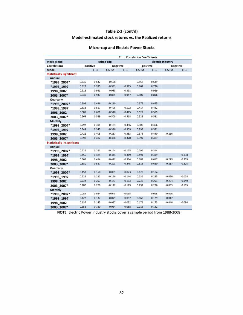
82

Table 2-2 (cont’d) Model-estimated stock returns vs. the Realized returns

Micro-cap and Electric Power Stocks

C. Correlation Coefficients Stock group Micro-cap Electric Industry Correlations positive negative positive negative Model ` FF3 CAPM FF3 CAPM FF3 CAPM FF3 Statistically Significant

Annual

*1993_2007* 0.635 0.642 -0.598 0.558 0.639

*1993_1997 0.927 0.935 -0.933 -0.915 0.764 0.736

1998_2002 0.913 0.931 -0.933 -0.898 0.929

2003_2007* 0.930 0.937 -0.885 -0.947 0.907 0.896

Quarterly

*1993_2007* 0.398 0.436 -0.280 0.375 0.455

*1993_1997 0.538 0.567 -0.495 -0.502 0.414 0.422

1998_2002 0.581 0.601 -0.510 -0.475 0.522 0.559

2003_2007* 0.569 0.589 -0.508 -0.518 0.523 0.581

Monthly

*1993_2007* 0.292 0.301 -0.184 -0.356 0.300 0.366

*1993_1997 0.344 0.343 -0.326 -0.309 0.298 0.381

1998_2002 0.422 0.405 -0.287 -0.383 0.373 0.440 -0.256

2003_2007* 0.398 0.402 -0.338 -0.320 0.397 0.407

Statistically Insignificant

Annual

*1993_2007* 0.225 0.291 -0.144 -0.175 0.296 0.314

*1993_1997 0.455 0.485 -0.344 -0.319 0.491 0.419 -0.138

1998_2002 0.369 0.454 -0.442 -0.364 0.381 0.617 -0.279 -0.305

2003_2007* 0.580 0.587 -0.293 -0.245 0.615 0.660 -0.217 -0.225

Quarterly

*1993_2007* 0.153 0.150 -0.089 -0.073 0.123 0.104

*1993_1997 0.224 0.232 -0.156 -0.144 0.236 0.235 -0.030 -0.028

1998_2002 0.234 0.257 -0.143 -0.133 0.232 0.291 -0.204 -0.140

2003_2007* 0.280 0.270 -0.142 -0.129 0.292 0.276 -0.035 -0.105

Monthly

*1993_2007* 0.084 0.084 -0.045 -0.055 0.098 -0.096

*1993_1997 0.122 0.137 -0.079 -0.087 0.163 0.129 -0.017

1998_2002 0.137 0.145 -0.087 -0.092 0.171 0.173 -0.040 -0.084

2003_2007* 0.156 0.160 -0.064 -0.088 0.015 0.122

NOTE: Electric Power Industry stocks cover a sample period from 1988-2008

83

Table 2-3-1 Model-estimated stock returns vs. the Realized returns

Fama-French 10 Industry and 25 Size/Value Portfolios

Columns A count the number of stocks or portfolios; Columns B estimate the correlation coefficients.

A. Count of Portfolios B. Correlation Coefficients Stock group F12 FF25 F12 FF25 Model CAPM FF3 CAPM FF3 CAPM FF3 CAPM FF3

Statistically Significant Annual

1963_2008 12 12 25 25 0.808 0.840 0.818 0.956

1963_1972 12 12 25 25 0.888 0.924 0.899 0.982

1973_1991 12 12 25 25 0.860 0.856 0.866 0.961

1992_2000 4 10 3 25 0.796 0.803 0.815 0.906

2001_2008 6 8 21 24 0.880 0.896 0.903 0.951

Quarterly

1963_2008 12 12 25 25 0.835 0.851 0.863 0.941

1963_1972 12 12 25 25 0.849 0.859 0.877 0.931

1973_1991 12 12 25 25 0.886 0.880 0.907 0.956

1992_2000 11 12 25 25 0.688 0.774 0.736 0.917

2001_2008 12 12 25 25 0.812 0.793 0.857 0.940

Monthly

1963_2008 12 12 25 25 0.814 0.819 0.878 0.958

1963_1972 12 12 25 25 0.842 0.812 0.900 0.962

1973_1991 12 12 25 25 0.865 0.859 0.926 0.970

1992_2000 12 12 25 25 0.654 0.739 0.688 0.931

2001_2008 12 12 25 25 0.771 0.766 0.868 0.952 Statistically Insignificant

Annual 1992_2000 8 2 15 0.492 0.413 0.330

2001_2008 6 4 4 1 0.573 0.553 0.720 0.661 Quarterly

1992_2000 1 0.203

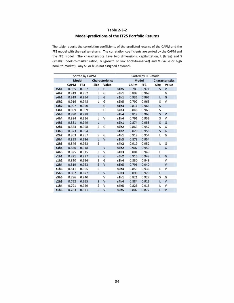
84

Table 2-3-2 Model-predictions of the FF25 Portfolio Returns

The table reports the correlation coefficients of the predicted returns of the CAPM and the FF3 model with the realize returns. The correlation coefficients are sorted by the CAPM and the FF3 model. The characteristics have two dimensions: capitalization, L (large) and S (small): book-to-market ration, G (growth or low book-to-market) and V (value or high book-to-market). Any S3 or h3 is not assigned a symbol.

Sorted by CAPM Sorted by FF3 model Model Characteristics Model Characteristics CAPM FF3 Size Value CAPM FF3 Size Value s5h1 0.935 0.967 L G s1h5 0.783 0.971 S V s4h2 0.919 0.952 L G s3h1 0.899 0.969 G s4h1 0.919 0.954 L G s5h1 0.935 0.967 L G s5h2 0.916 0.948 L G s2h5 0.792 0.965 S V s3h2 0.907 0.950 G s1h3 0.811 0.965 S s3h1 0.899 0.969 G s2h3 0.846 0.963 S s5h3 0.890 0.928 L s2h4 0.819 0.963 S V s4h4 0.884 0.916 L V s1h4 0.791 0.959 S V s4h3 0.881 0.949 L s2h1 0.874 0.958 S G s2h1 0.874 0.958 S G s2h2 0.863 0.957 S G s3h3 0.873 0.954 s1h2 0.820 0.956 S G s2h2 0.863 0.957 S G s4h1 0.919 0.954 L G s5h4 0.853 0.936 L V s3h3 0.873 0.954 s2h3 0.846 0.963 S s4h2 0.919 0.952 L G s3h4 0.830 0.948 V s3h2 0.907 0.950 G s4h5 0.825 0.915 L V s4h3 0.881 0.949 L s1h1 0.821 0.927 S G s5h2 0.916 0.948 L G s1h2 0.820 0.956 S G s3h4 0.830 0.948 V s2h4 0.819 0.963 S V s3h5 0.796 0.940 V s1h3 0.811 0.965 S s5h4 0.853 0.936 L V s5h5 0.802 0.877 L V s5h3 0.890 0.928 L s3h5 0.796 0.940 V s1h1 0.821 0.927 S G s2h5 0.792 0.965 S V s4h4 0.884 0.916 L V s1h4 0.791 0.959 S V s4h5 0.825 0.915 L V s1h5 0.783 0.971 S V s5h5 0.802 0.877 L V

85

Table 2-4-1 F-tests for Equality of Mean Squared Errors (MSEs)

This table reports the F-test results for the equality of MSEs of the CAPM and the Fama-French 3-factor model. Five-year Rolling regressions are conducted on monthly stock returns. The MSEs are calculated on one-period or one-month-ahead prediction for each rolling regression. The following stocks with full history for 1988-2008 are tested: 28 Dow Jones stocks, 315 Large-cap or S&P500 stocks, and 204 Russell 2000 Micro-cap stocks..

Dow Jones Large-cap Micro-cap equal unequal equal unequal equal

Total 191 1 190 2 192 1993 12 12 12 1994 12 12 12 1995 12 12 12 1996 12 12 12 1997 12 12 12 1998 12 12 12 1999 12 12 12 2000 11 1 11 1 12 2001 12 11 1 12 2002 12 12 12 2003 12 12 12 2004 12 12 12 2005 12 12 12 2006 12 12 12 2007 12 12 12 2008 12 12 12

86

Table 2-4-2 Rolling Regression Specifications

The model specifications of rolling regressions are similar to those of the test using daily return data. The market index is the most significant load factor among three risk factors for individual stocks and the FF25 portfolios. For individual stocks, the market index is the most significant factor by itself. However, for two thirds of the FF25 portfolios, all three factors are jointly significant.

Significant Estimates Alpha is insignificant No risk factors

are significant

Alpha is significant

Total

Beta SMB HML

1 2 3 4 5 6 7

Beta X X X X

SMB X X X X HML X X X X

Micro-cap Stocks

0.363

CAPM 14230

23526 1412 39168 0.316 0.257 0.144 FF3 6902 2260 1438 1781 1033 5316 1404 17758 1276 39168

% 0.176 0.058 0.037 0.045 0.026 0.136 0.036 0.453 0.033 1.000

Large-cap Stocks

0.774 CAPM 46833 10102 3545 60480 0.828 0.204 0.337 FF3 23759 7619 3434 15279 322 986 1353 4197 3531 60480 % 0.393 0.126 0.057 0.253 0.005 0.016 0.022 0.069 0.058 1

Dow Jones Index Stocks

0.876 CAPM 4710 427 239 5376 0.850 0.323 0.290 FF3 1875 1189 389 1119 12 145 37 195 415 5376 % 0.349 0.221 0.072 0.208 0.002 0.027 0.007 0.036 0.077 1

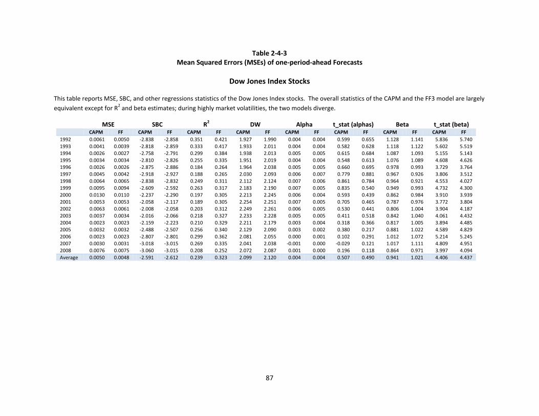
87

Table 2-4-3 Mean Squared Errors (MSEs) of one-period-ahead Forecasts

Dow Jones Index Stocks

This table reports MSE, SBC, and other regressions statistics of the Dow Jones Index stocks. The overall statistics of the CAPM and the FF3 model are largely equivalent except for R2 and beta estimates; during highly market volatilities, the two models diverge.

MSE SBC R2 DW Alpha t_stat (alphas) Beta t_stat (beta)

CAPM FF CAPM FF CAPM FF CAPM FF CAPM FF CAPM FF CAPM FF CAPM FF

1992 0.0061 0.0050 -2.838 -2.858 0.351 0.421 1.927 1.990 0.004 0.004 0.599 0.655 1.128 1.141 5.836 5.740 1993 0.0041 0.0039 -2.818 -2.859 0.333 0.417 1.933 2.011 0.004 0.004 0.582 0.628 1.118 1.122 5.602 5.519 1994 0.0026 0.0027 -2.758 -2.791 0.299 0.384 1.938 2.013 0.005 0.005 0.615 0.684 1.087 1.093 5.155 5.143 1995 0.0034 0.0034 -2.810 -2.826 0.255 0.335 1.951 2.019 0.004 0.004 0.548 0.613 1.076 1.089 4.608 4.626 1996 0.0026 0.0026 -2.875 -2.886 0.184 0.264 1.964 2.038 0.005 0.005 0.660 0.695 0.978 0.993 3.729 3.764 1997 0.0045 0.0042 -2.918 -2.927 0.188 0.265 2.030 2.093 0.006 0.007 0.779 0.881 0.967 0.926 3.806 3.512 1998 0.0064 0.0065 -2.838 -2.832 0.249 0.311 2.112 2.124 0.007 0.006 0.861 0.784 0.964 0.921 4.553 4.027 1999 0.0095 0.0094 -2.609 -2.592 0.263 0.317 2.183 2.190 0.007 0.005 0.835 0.540 0.949 0.993 4.732 4.300 2000 0.0130 0.0110 -2.237 -2.290 0.197 0.305 2.213 2.245 0.006 0.004 0.593 0.439 0.862 0.984 3.910 3.939 2001 0.0053 0.0053 -2.058 -2.117 0.189 0.305 2.254 2.251 0.007 0.005 0.705 0.465 0.787 0.976 3.772 3.804 2002 0.0063 0.0061 -2.008 -2.058 0.203 0.312 2.249 2.261 0.006 0.005 0.530 0.441 0.806 1.004 3.904 4.187 2003 0.0037 0.0034 -2.016 -2.066 0.218 0.327 2.233 2.228 0.005 0.005 0.411 0.518 0.842 1.040 4.061 4.432 2004 0.0023 0.0023 -2.159 -2.223 0.210 0.329 2.211 2.179 0.003 0.004 0.318 0.366 0.817 1.005 3.894 4.485 2005 0.0032 0.0032 -2.488 -2.507 0.256 0.340 2.129 2.090 0.003 0.002 0.380 0.217 0.881 1.022 4.589 4.829 2006 0.0023 0.0023 -2.807 -2.801 0.299 0.362 2.081 2.055 0.000 0.001 0.102 0.291 1.012 1.072 5.214 5.245 2007 0.0030 0.0031 -3.018 -3.015 0.269 0.335 2.041 2.038 -0.001 0.000 -0.029 0.121 1.017 1.111 4.809 4.951 2008 0.0076 0.0075 -3.060 -3.015 0.208 0.252 2.072 2.087 0.001 0.000 0.196 0.118 0.864 0.971 3.997 4.094 Average 0.0050 0.0048 -2.591 -2.612 0.239 0.323 2.099 2.120 0.004 0.004 0.507 0.490 0.941 1.021 4.406 4.437

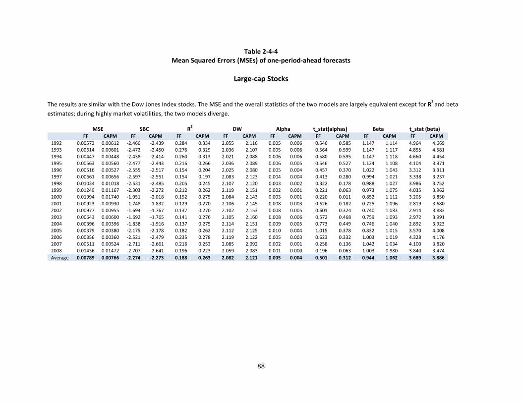
88

Table 2-4-4 Mean Squared Errors (MSEs) of one-period-ahead forecasts

Large-cap Stocks

The results are similar with the Dow Jones Index stocks. The MSE and the overall statistics of the two models are largely equivalent except for R2 and beta estimates; during highly market volatilities, the two models diverge.

MSE SBC R2 DW Alpha t_stat(alphas) Beta t_stat (beta)

FF CAPM FF CAPM FF CAPM FF CAPM FF CAPM FF CAPM FF CAPM FF CAPM 1992 0.00573 0.00612 -2.466 -2.439 0.284 0.334 2.055 2.116 0.005 0.006 0.546 0.585 1.147 1.114 4.964 4.669 1993 0.00614 0.00601 -2.472 -2.450 0.276 0.329 2.036 2.107 0.005 0.006 0.564 0.599 1.147 1.117 4.855 4.581 1994 0.00447 0.00448 -2.438 -2.414 0.260 0.313 2.021 2.088 0.006 0.006 0.580 0.595 1.147 1.118 4.660 4.454 1995 0.00563 0.00560 -2.477 -2.443 0.216 0.266 2.036 2.089 0.006 0.005 0.546 0.527 1.124 1.108 4.104 3.971 1996 0.00516 0.00527 -2.555 -2.517 0.154 0.204 2.025 2.080 0.005 0.004 0.457 0.370 1.022 1.043 3.312 3.311 1997 0.00661 0.00656 -2.597 -2.551 0.154 0.197 2.083 2.123 0.004 0.004 0.413 0.280 0.994 1.021 3.338 3.237 1998 0.01034 0.01018 -2.531 -2.485 0.205 0.245 2.107 2.120 0.003 0.002 0.322 0.178 0.988 1.027 3.986 3.752 1999 0.01249 0.01167 -2.303 -2.272 0.212 0.262 2.119 2.151 0.002 0.001 0.221 0.063 0.973 1.075 4.035 3.962 2000 0.01994 0.01740 -1.951 -2.018 0.152 0.275 2.084 2.143 0.003 0.001 0.220 0.011 0.852 1.112 3.205 3.850 2001 0.00923 0.00930 -1.748 -1.832 0.129 0.270 2.106 2.145 0.008 0.003 0.626 0.182 0.725 1.096 2.819 3.680 2002 0.00977 0.00955 -1.694 -1.767 0.137 0.270 2.102 2.153 0.008 0.005 0.601 0.324 0.740 1.083 2.914 3.883 2003 0.00643 0.00600 -1.692 -1.765 0.141 0.276 2.105 2.160 0.008 0.006 0.572 0.468 0.759 1.093 2.972 3.991 2004 0.00396 0.00396 -1.838 -1.916 0.137 0.275 2.114 2.151 0.009 0.005 0.773 0.449 0.746 1.040 2.892 3.923 2005 0.00379 0.00380 -2.175 -2.178 0.182 0.262 2.112 2.125 0.010 0.004 1.015 0.378 0.832 1.015 3.570 4.008 2006 0.00356 0.00360 -2.521 -2.479 0.235 0.278 2.119 2.122 0.005 0.003 0.623 0.332 1.003 1.019 4.328 4.176 2007 0.00511 0.00524 -2.711 -2.661 0.216 0.253 2.085 2.092 0.002 0.001 0.258 0.136 1.042 1.034 4.100 3.820 2008 0.01436 0.01472 -2.707 -2.641 0.196 0.223 2.059 2.083 0.001 0.000 0.196 0.063 1.003 0.980 3.840 3.474 Average 0.00789 0.00766 -2.274 -2.273 0.188 0.263 2.082 2.121 0.005 0.004 0.501 0.312 0.944 1.062 3.689 3.886

89

Table 2-4-5 Mean Squared Errors (MSEs) of one-period-ahead forecasts

Micro-cap Stocks

The MSE and the overall statistics of the two models are largely equivalent except for R2 and beta estimates; during highly market volatilities, the two models diverge. However, the MSEs of both models are higher, the SBCs worse, and the R2 lower than large-cap stocks, whose statistics are poorer than those of DJ Index stocks. The variability of MSEs may be the main reason for the statistical equivalence of the two models.

MSE SBC R2 DW Alpha t-statistic (alphas)

Beta t-statistic

(beta) FF CAPM FF CAPM FF CAPM FF CAPM FF CAPM FF CAPM FF CAPM FF CAPM 1992 0.0302 0.0313 -1.289 -1.250 0.053 0.108 2.051 2.120 0.006 0.005 0.212 0.179 0.742 0.746 1.668 1.616 1993 0.0315 0.0334 -1.271 -1.239 0.052 0.112 2.053 2.134 0.006 0.006 0.248 0.234 0.722 0.715 1.610 1.543 1994 0.0191 0.0207 -1.245 -1.210 0.049 0.106 2.065 2.136 0.008 0.007 0.323 0.258 0.725 0.640 1.586 1.392 1995 0.0230 0.0234 -1.235 -1.191 0.038 0.088 2.077 2.139 0.011 0.007 0.467 0.272 0.698 0.661 1.342 1.257 1996 0.0255 0.0268 -1.287 -1.237 0.019 0.065 2.052 2.113 0.012 0.007 0.566 0.318 0.545 0.634 0.903 1.020 1997 0.0294 0.0287 -1.366 -1.296 0.026 0.054 2.071 2.118 0.007 0.006 0.377 0.244 0.704 0.739 1.195 1.218 1998 0.0299 0.0306 -1.382 -1.311 0.041 0.067 2.097 2.129 0.004 0.006 0.181 0.247 0.673 0.666 1.473 1.355 1999 0.0433 0.0425 -1.295 -1.236 0.051 0.088 2.118 2.170 0.000 0.005 -0.079 0.119 0.700 0.699 1.688 1.552 2000 0.0530 0.0473 -1.095 -1.073 0.043 0.109 2.103 2.167 0.004 0.006 0.048 0.081 0.656 0.705 1.536 1.616 2001 0.0259 0.0280 -1.001 -0.980 0.050 0.114 2.133 2.187 0.005 0.005 0.183 0.073 0.695 0.662 1.682 1.555 2002 0.0301 0.0312 -0.982 -0.956 0.054 0.114 2.134 2.187 0.008 0.005 0.276 0.091 0.698 0.653 1.726 1.639 2003 0.0294 0.0288 -0.981 -0.947 0.055 0.108 2.148 2.188 0.012 0.007 0.465 0.213 0.724 0.684 1.722 1.639 2004 0.0251 0.0251 -1.056 -1.015 0.059 0.106 2.124 2.146 0.018 0.011 0.870 0.447 0.791 0.711 1.777 1.643 2005 0.0192 0.0190 -1.236 -1.173 0.076 0.107 2.136 2.145 0.015 0.010 0.904 0.463 0.855 0.729 2.065 1.603 2006 0.0157 0.0160 -1.386 -1.314 0.066 0.091 2.115 2.130 0.012 0.006 0.693 0.265 0.856 0.776 1.925 1.623 2007 0.0192 0.0195 -1.479 -1.398 0.054 0.071 2.089 2.111 0.006 0.004 0.356 0.172 0.920 0.727 1.751 1.293 2008 0.0324 0.0348 -1.489 -1.404 0.063 0.077 2.095 2.123 0.001 0.000 -0.039 -0.129 0.974 0.761 1.930 1.431 Average 0.0280 0.0280 -1.236 -1.185 0.050 0.093 2.100 2.145 0.008 0.006 0.366 0.212 0.745 0.698 1.618 1.462

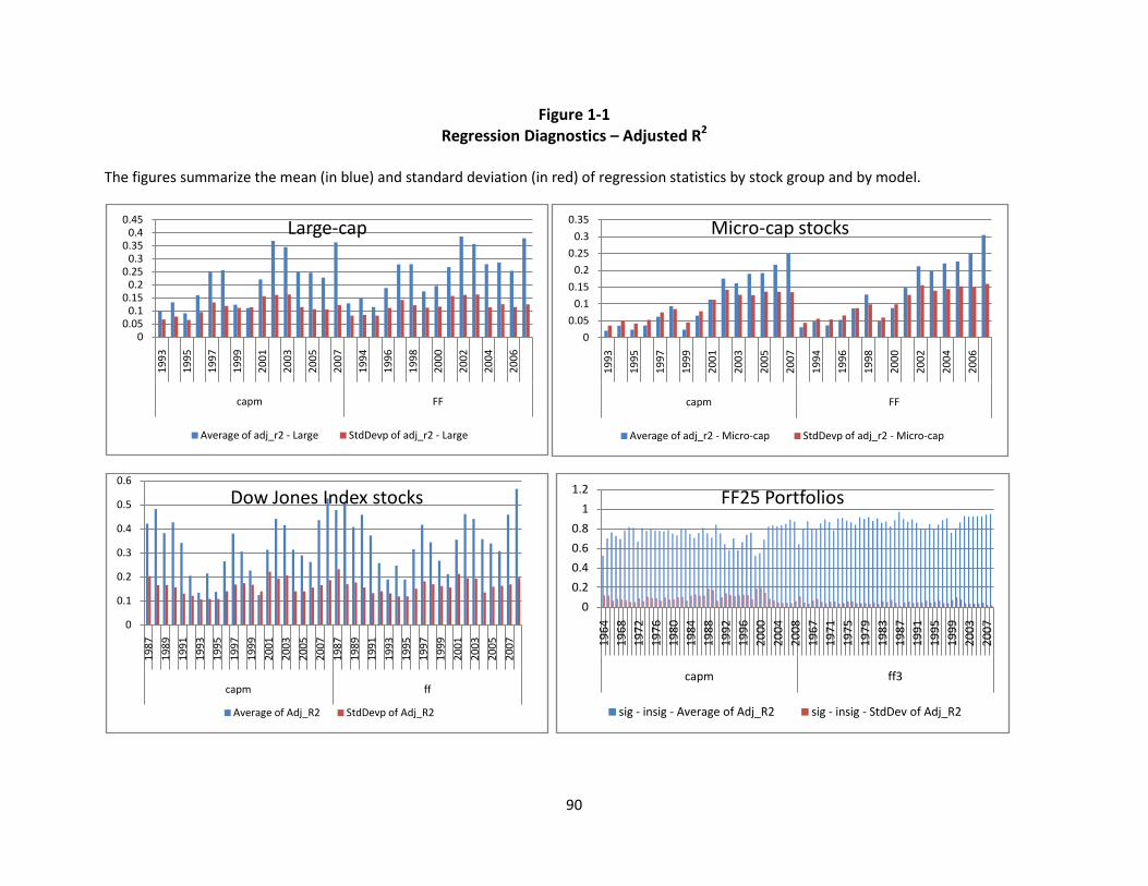
90

Figure 1-1 Regression Diagnostics – Adjusted R2

The figures summarize the mean (in blue) and standard deviation (in red) of regression statistics by stock group and by model.

00.05

0.10.15

0.20.25

0.30.35

0.40.45

1993

1995

1997

1999

2001

2003

2005

2007

1994

1996

1998

2000

2002

2004

2006

capm FF

Large-cap

Average of adj_r2 - Large StdDevp of adj_r2 - Large

0

0.05

0.1

0.15

0.2

0.25

0.3

0.35

1993

1995

1997

1999

2001

2003

2005

2007

1994

1996

1998

2000

2002

2004

2006

capm FF

Micro-cap stocks

Average of adj_r2 - Micro-cap StdDevp of adj_r2 - Micro-cap

0

0.1

0.2

0.3

0.4

0.5

0.6

1987

1989

1991

1993

1995

1997

1999

2001

2003

2005

2007

1987

1989

1991

1993

1995

1997

1999

2001

2003

2005

2007

capm ff

Dow Jones Index stocks

Average of Adj_R2 StdDevp of Adj_R2

0

0.2

0.4

0.6

0.8

1

1.2

1964

1968

1972

1976

1980

1984

1988

1992

1996

2000

2004

2008

1967

1971

1975

1979

1983

1987

1991

1995

1999

2003

2007

capm ff3

FF25 Portfolios

sig - insig - Average of Adj_R2 sig - insig - StdDev of Adj_R2

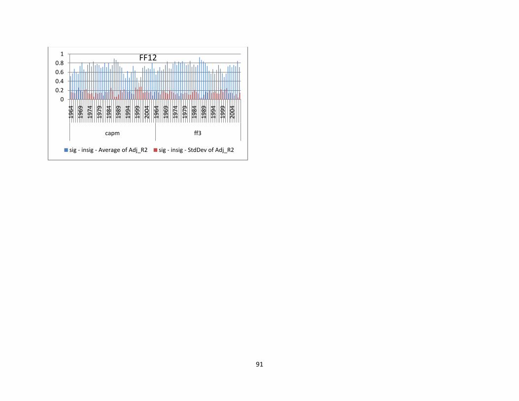
91

00.20.40.60.8

1

1964

1969

1974

1979

1984

1989

1994

1999

2004

1964

1969

1974

1979

1984

1989

1994

1999

2004

capm ff3

FF12

sig - insig - Average of Adj_R2 sig - insig - StdDev of Adj_R2

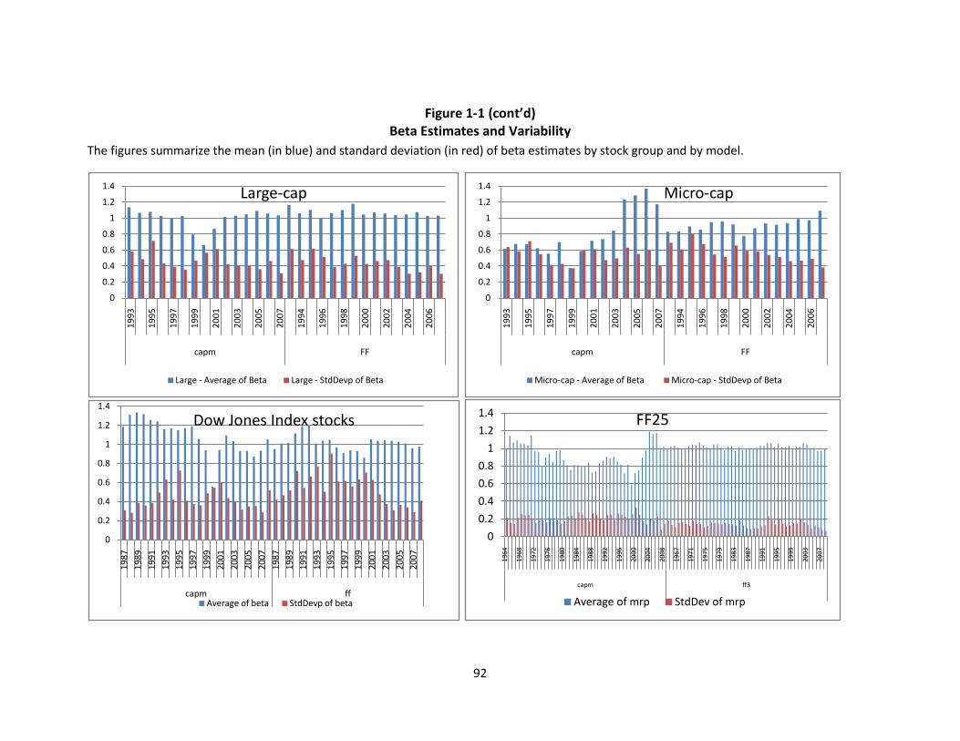
92

Figure 1-1 (cont’d) Beta Estimates and Variability

The figures summarize the mean (in blue) and standard deviation (in red) of beta estimates by stock group and by model.

0

0.2

0.4

0.6

0.8

1

1.2

1.4

1993

1995

1997

1999

2001

2003

2005

2007

1994

1996

1998

2000

2002

2004

2006

capm FF

Large-cap

Large - Average of Beta Large - StdDevp of Beta

0

0.2

0.4

0.6

0.8

1

1.2

1.4

1993

1995

1997

1999

2001

2003

2005

2007

1994

1996

1998

2000

2002

2004

2006

capm FF

Micro-cap

Micro-cap - Average of Beta Micro-cap - StdDevp of Beta

0

0.2

0.4

0.6

0.8

1

1.2

1.4

1987

1989

1991

1993

1995

1997

1999

2001

2003

2005

2007

1987

1989

1991

1993

1995

1997

1999

2001

2003

2005

2007

capm ff

Dow Jones Index stocks

Average of beta StdDevp of beta

0

0.2

0.4

0.6

0.8

1

1.2

1.4

1964

1968

1972

1976

1980

1984

1988

1992

1996

2000

2004

2008

1967

1971

1975

1979

1983

1987

1991

1995

1999

2003

2007

capm ff3

FF25

Average of mrp StdDev of mrp

93

00.20.40.60.8

11.21.4

1964

1968

1972

1976

1980

1984

1988

1992

1996

2000

2004

2008

1967

1971

1975

1979

1983

1987

1991

1995

1999

2003

2007

capm ff3

FF12

sig - insig - Average of mrp sig - insig - StdDev of mrp

94

Supplementary Exhibits to

Tables 1-1-1 and 1-1-2

These exhibits report inter-temporal shifts of the factor loadings on individual stock groups and the Fama-French portfolios. The exhibits show the percentages of regressions of a variety of combinations of significant risk factors in each stock or portfolio group. Legend - Examples “Sig-insig-insig-insig” represents that the market beta is significant, but the alpha, SMB, and HML estimates are insignificant. This is Specification 1, where the market beta is solely significant. (“Market Beta”) The focus is the number of regressions where the market index is significant alone or in combination with SMB or HML. There are four combinations where the market index is significant: Specifications 1 through 4

• Specification 1: The Market index is solely significant (“Market Beta”) in blue color at the bottom

• Specification 2: The market index and SMB are significant (Beta+SMB or “Sig-insig-sig-insig”) in red color stacked on Specification 1

• Specification 3: The market index, SMB, an HML are significant. (Beta+SMB+HML or “Sig-insig-sig-sig”) in green color stacked on Specification 2

• Specification 4: The market index and HML are significant (Beta+HML or “Sig-insig-insig-sig”) in purple color stacked on Specification 3

Specifications 5 through 7 report significant SMB or HML loadings, or a combination of two significant factors.

• Specification 5: SMB and HML are significant (“insig-insig-sig-sig”) • Specification 6: SMB is solely significant (“insig-insig-sig-insig”) • Specification 7: HML is solely significant (“insig-insig-insig-sig”)

Specification 8 reports where all risk factors and alpha estimates are insignificant.

• Specification 8: No factor loading is significant (“insig-insig-insig-insig”) Specification9 reports where alpha estimates are significant whether or not a factor loading is significant. Therefore, Specifications 1 through 8 contains only the regressions whose alpha estimates are insignificant.

• Specification 9: No factor loading is significant (“insig-insig-insig-insig”)

95

Exhibit to Tables 1-1-1 and 1-1-2

Micro-cap Stocks

A. Annual Estimation

B. Quarterly Estimation

0%

10%

20%

30%

40%

50%

60%

70%

80%

90%

100%

1993

1994

1995

1996

1997

1998

1999

2000

2001

2002

2003

2004

2005

2006

2007

FF

Micro-cap - insig - sig - sig - sig

Micro-cap - insig - sig - sig - insig

Micro-cap - insig - sig - insig - sig

Micro-cap - insig - sig - insig - insig

Micro-cap - insig - insig - sig - sig

Micro-cap - insig - insig - sig - insig

Micro-cap - insig - insig - insig - sig

Micro-cap - insig - insig - insig - insig

Micro-cap - sig - sig - sig - sig

Micro-cap - sig - sig - sig - insig

Micro-cap - sig - sig - insig - sig

Micro-cap - sig - sig - insig - insig

Micro-cap - sig - insig - sig - sig

Micro-cap - sig - insig - sig - insig

Micro-cap - sig - insig - insig - sig

Micro-cap - sig - insig - insig - insig

Beta+SMB

No factor is significant

Market Beta

Beta +HML

Beta+SMB+HML

Beta+HML

0%

10%

20%

30%

40%

50%

60%

70%

80%

90%

100%

1993 1994 1995 1996 1997 1998 1999 2000 2001 2002 2003 2004 2005 2006 2007

ff

insig - sig - sig - sig

insig - sig - sig - insig

insig - sig - insig - sig

insig - sig - insig - insig

insig - insig - sig - sig

insig - insig - sig - insig

insig - insig - insig - sig

insig - insig - insig - insig

sig - sig - sig - sig

sig - sig - sig - insig

sig - sig - insig - sig

sig - sig - insig - insig

sig - insig - sig - sig

sig - insig - sig - insig

sig - insig - insig - sig

No factor is significant

Market Beta

Beta +HML

Beta+SMB

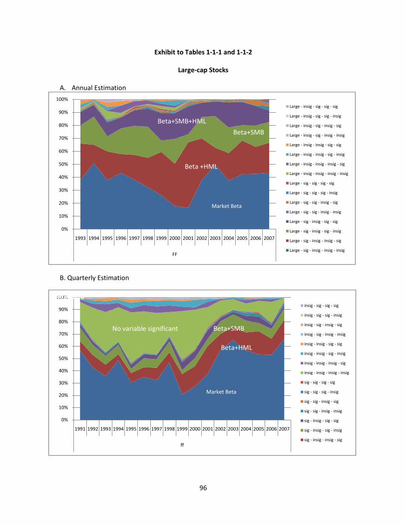
96

Exhibit to Tables 1-1-1 and 1-1-2

Large-cap Stocks

A. Annual Estimation

B. Quarterly Estimation

0%

10%

20%

30%

40%

50%

60%

70%

80%

90%

100%

1993 1994 1995 1996 1997 1998 1999 2000 2001 2002 2003 2004 2005 2006 2007

FF

Large - insig - sig - sig - sig

Large - insig - sig - sig - insig

Large - insig - sig - insig - sig

Large - insig - sig - insig - insig

Large - insig - insig - sig - sig

Large - insig - insig - sig - insig

Large - insig - insig - insig - sig

Large - insig - insig - insig - insig

Large - sig - sig - sig - sig

Large - sig - sig - sig - insig

Large - sig - sig - insig - sig

Large - sig - sig - insig - insig

Large - sig - insig - sig - sig

Large - sig - insig - sig - insig

Large - sig - insig - insig - sig

Large - sig - insig - insig - insig

Market Beta

Beta +HML

Beta+SMB

Beta+SMB+HML

0%

10%

20%

30%

40%

50%

60%

70%

80%

90%

100%

1991 1992 1993 1994 1995 1996 1997 1998 1999 2000 2001 2002 2003 2004 2005 2006 2007

ff

insig - sig - sig - sig

insig - sig - sig - insig

insig - sig - insig - sig

insig - sig - insig - insig

insig - insig - sig - sig

insig - insig - sig - insig

insig - insig - insig - sig

insig - insig - insig - insig

sig - sig - sig - sig

sig - sig - sig - insig

sig - sig - insig - sig

sig - sig - insig - insig

sig - insig - sig - sig

sig - insig - sig - insig

sig - insig - insig - sig

Market Beta

Market Beta

Market Beta

No variable significant

Beta+HML

Beta+SMB

Beta+SMB

97

Appendix to Tables 1-1-1 and 1-1-2

Dow Jones Stocks A. Annual Estimation

B. Quarterly Estimation

0%

10%

20%

30%

40%

50%

60%

70%

80%

90%

100%

1987

1988

1989

1990

1991

1992

1993

1994

1995

1996

1997

1998

1999

2000

2001

2002

2003

2004

2005

2006

2007

2008

ff

insig - sig - sig - sig

insig - insig - sig - sig

insig - insig - sig - insig

insig - insig - insig - sig

sig - sig - sig - sig

sig - sig - sig - insig

sig - sig - insig - sig

sig - sig - insig - insig

sig - insig - sig - sig

sig - insig - sig - insig

sig - insig - insig - sig

sig - insig - insig - insig

Market Beta

MarketBetaMarketBetaMarketBeta

Beta+HML

Beta+SMB

Beta+SMB+HML

0%

10%

20%

30%

40%

50%

60%

70%

80%

90%

100%

1987

1988

1989

1990

1991

1992

1993

1994

1995

1996

1997

1998

1999

2000

2001

2002

2003

2004

2005

2006

2007

2008

ff

insig - sig - sig - sig

insig - sig - sig - insig

insig - sig - insig - sig

insig - sig - insig - insig

insig - insig - sig - sig

insig - insig - sig - insig

insig - insig - insig - sig

insig - insig - insig - insig

sig - sig - sig - sig

sig - sig - sig - insig

sig - sig - insig - sig

sig - sig - insig - insig

sig - insig - sig - sig

sig - insig - sig - insig

sig - insig - insig - sig

sig - insig - insig - insig

No variable significant

Market Beta

Beta+SMB

98

Appendix to Tables 1-1-1 and 1-1-2

Fama-French 12 Industry Portfolio A. Annual Estimation

B. Quarterly estimation

0%

10%

20%

30%

40%

50%

60%

70%

80%

90%

100%

1964

1966

1968

1970

1972

1974

1976

1978

1980

1982

1984

1986

1988

1990

1992

1994

1996

1998

2000

2002

2004

2006

2008

ff3

sig - sig - sig - sig

sig - sig - sig - insig

sig - sig - insig - sig

sig - sig - insig - insig

sig - insig - sig - sig

sig - insig - sig - insig

sig - insig - insig - sig

sig - insig - insig - insig

Beta+SMB+HML

Beta+SMB

0%

10%

20%

30%

40%

50%

60%

70%

80%

90%

100%

1963

1965

1967

1969

1971

1973

1975

1977

1979

1981

1983

1985

1987

1989

1991

1993

1995

1997

1999

2001

2003

2005

2007

ff

insig - sig - sig - insig

insig - sig - insig - insig

insig - insig - sig - sig

insig - insig - sig - insig

insig - insig - insig - sig

insig - insig - insig - insig

sig - sig - sig - insig

sig - sig - insig - sig

sig - sig - insig - insig

sig - insig - sig - sig

sig - insig - sig - insig

sig - insig - insig - sig

Market Beta

Beta+SMB

99

Appendix to Tables 1-1-1 and 1-1-2

FF25 Portfolio

0%

10%

20%

30%

40%

50%

60%

70%

80%

90%

100%

1964

1966

1968

1970

1972

1974

1976

1978

1980

1982

1984

1986

1988

1990

1992

1994

1996

1998

2000

2002

2004

2006

2008

ff3

A. Annual Estimation - FF25 Portfolio

sig - sig - sig - sig

sig - sig - sig - insig

sig - sig - insig - sig

sig - sig - insig - insig

sig - insig - sig - sig

sig - insig - sig - insig

sig - insig - insig - sig

sig - insig - insig - insig

Beta+SMB+HML

Beta+SMB

0%

10%

20%

30%

40%

50%

60%

70%

80%

90%

100%

1963

1965

1967

1969

1971

1973

1975

1977

1979

1981

1983

1985

1987

1989

1991

1993

1995

1997

1999

2001

2003

2005

2007

ff

B. Quarterly estimation - FF25 Portfolio

sig - sig - sig - sig

sig - sig - sig - insig

sig - sig - insig - sig

sig - sig - insig - insig

sig - insig - sig - sig

sig - insig - sig - insig

sig - insig - insig - sig

sig - insig - insig - insig

Beta+SMB+HMLBeta+SMB+HML

Beta+SMB+HML

Beta+SMB

100

Appendix to Tables 1-1-1 and 1-1-2

FF25 Portfolio – cross-sectional

C. Annual estimation – cross-sectional

D. Quarterly estimation – cross-sectional

0%

10%

20%

30%

40%

50%

60%

70%

80%

90%

100%

s1h1

s1h2

s1h3

s1h4

s1h5

s2h1

s2h2

s2h3

s2h4

s2h5

s3h1

s3h2

s3h3

s3h4

s3h5

s4h1

s4h2

s4h3

s4h4

s4h5

s5h1

s5h2

s5h3

s5h4

s5h5

ff3

sig - sig - sig - sig

sig - sig - sig - insig

sig - sig - insig - sig

sig - sig - insig - insig

sig - insig - sig - sig

sig - insig - sig - insig

sig - insig - insig - sig

sig - insig - insig - insig

Beta+SMB+HML

Beta+SMB

0%

10%

20%

30%

40%

50%

60%

70%

80%

90%

100%

s1h1

s1h2

s1h3

s1h4

s1h5

s2h1

s2h2

s2h3

s2h4

s2h5

s3h1

s3h2

s3h3

s3h4

s3h5

s4h1

s4h2

s4h3

s4h4

s4h5

s5h1

s5h2

s5h3

s5h4

s5h5

ff

sig - sig - sig - sig

sig - sig - sig - insig

sig - sig - insig - sig

sig - sig - insig - insig

sig - insig - sig - sig

sig - insig - sig - insig

sig - insig - insig - sig

sig - insig - insig - insig

Beta+SMB+HML

Beta+SMB

101

Chapter 3

Industry Restructuring, Market Risk, and the Cost of Capital: A case study of electric power industry deregulation

Chapter 3 presents the results of a focused test on the firms of the electric power industry, which has been going through a restructuring and deregulation process since the 1990s. The main objective of this chapter is to test for inter-temporal and cross-sectional regime-shift of beta and to identify the economic sources of the shift, as the market and industry environment changes and a firm’s investment model and financing strategy evolve. To gain conditioning information, I examine the industry restructuring process at the market, government policy and corporate investment and financing strategy levels. The information provides a basis for the design of research and the sample data and also for economic interpretation of test results. Based on the conditioning information, I divide the test sample period (1988-2008) into subsamples and the test results of individual firms are grouped by investment model and financing strategy (competitive vs. traditional utility business). Most of the findings in Chapter 2 also apply to the electric power industry. Additional major findings specific to the industry include the following: The test rejects the hypothesis that the regime of market beta has remained unchanged. The structural break tests show that the industry beta appears to have shifted its regime in 2002 during the restructuring process and at the height of the industry crisis. The beta estimates of the competitive business cross-sectionally moved away from those firms which largely remained in the traditional utility business. The investigation finds strong and direct evidence that investment model and financing strategy of a firm affect stock prices and the market beta. The test results largely confirm the usefulness and importance of conditioning information in asset pricing model test and application for the estimation of the cost of equity capital.

102

1. Industry Restructuring and Market Risk The electric power industry has been undergoing a restructuring process to deregulate its power

generation and wholesale power marketing sector since the mid-1990s.63 Through a focused investigation

into a natural experiment of a specific industry and the firms, I attempt to identify inter-temporal and

cross-sectional factors that potentially impact the market risk of firms and the industry, and test for

regime-shift of the market betas.64

Under the cost-plus regulation, electric utility firms are allowed to largely recover the total costs

through electricity rates charged to retail customers. A regulated firm can be more protected from

competition than a monopolist in a competitive market; the former can sustain long-term loss because of

cost recovery clause, while the latter cannot (Averch and Johnson, 1962, p.1058). In a competitive

electric power market, the electric power industry is exposed to two market-related risks. Two major

costs in electric power business are the capital cost and the fuel cost: the former for the capital-intensive

generating and infrastructure facilities (transmission and distribution lines to each house, commercial, and

industrial entities) and the latter to generate electricity. Each cost takes up to 40 percent of total

production cost.

A natural question in testing CAPM betas on the restructuring of the electric power industry is

whether deregulation and market-based competition generally increases the market risk for an industry

and its individual firms. Industry regulation is often designed to expose firms to the market risk. (Grout

and Zalewska, 2006) The main intent of restructuring and deregulation is to foster competition and

efficiency; the main rationale of deregulation rests on a market-based competition of the public interest.

(Horowitz, 1986, pp.148, 149) Norton (1985) finds that an electric power firm in a state of heavier

regulation is less exposed to systematic risk than a firm with lighter regulation. Breen and Lerner (1972)

observe that strategic and operational management decisions, made in response to changing external

factors, affect a firm’s risk characteristics and its beta value.

65

63 The Appendix at the end of this chapter provides a brief background of the electric industry restructuring that has been taking shape since the 1990s. Advance review of the Appendix would provide a perspective to understand the discussion and test results of this chapter. 64 Grout and Zalewske (2006, p.151) note that changes in regulation provides a “clean” case that isolates the risk effect. While recognizing that natural experiments help “reduce the number of un-testable assumptions …and limit the range of alternative interpretations,” on the other hand, Rosenzweig and Wolpin (2000) argue that many of such studies do not produce easily generalizable results because the assumption of randomness is not credible. 65 Electric power supply business possible takes a long time to develop, incurs high cost, and bears regulatory risks. A large, base-demand power plant of one million KW generating capacity often costs one billion dollars and takes up to 10 years from the planning stage to commercial operation. In addition, construction process passes through a long series of hearings and approvals of federal, state, and local regulatory bodies and the community where a plant is to be located.

As a capital-intensive industry, electric power supply business is highly sensitive to

capital financing cost or interest rates. High financial leverage further increases the market risk of the

103

capital cost (Braun and Larrain, 2004). Under a restructured competitive market, firms heavily rely on

external financing to seize upon new business opportunities without an assurance to recover the cost,

while being subject to the vicissitudes of uncertain input factor or fuel cost, electricity or output prices,

profitability, market demand and revenues, and financing cost. Hamada (1972) finds that a firm’s

financial leverage has significant effects on the firm’s systematic risk of common stocks. Robicheck et al.

(1973) specifically find “stable and statistically significant” impact of financial leverage on the cost of

equity capital of electric utility firms.

Under full regulation, firms also are allowed to pass through fuel cost (“fuel adjustment clause”

or FAC) and thus were largely protected from the volatilities of fuel cost.66

2. Research Design for Beta Stationarity Test

Unable to pass through fuel

cost in a competitive market, merchant power generation and wholesale marketing firms become exposed

to volatilities of fuel cost, particularly natural gas prices which are often at the mercy of economic,

political, and market factors. Clarke (1980) finds that the FAC under regulation protects electric power

firms from systematic risk and market value.

Another natural question is whether the test results on an industry-specific deregulation process

can be applied to other industries. Economic studies usually suffer from the lack of laboratory

experiments which provide direct and repeated tests on the impact of a factor, separated from and

independent of other control factors. Chen, Roll, and Ross (1986) even argue that all economic variables

are endogenous and only natural forces are truly exogenous. Nevertheless, other deregulated industries,

such as telecommunications and airlines, had undergone a similar pattern such as overinvestment, high

financial leverage, and industry crisis in the wake of deregulation. The electric power industry proved no

exception. I argue that the focused study on the electric power industry offers managers of other

industries a framework for and an insight into how they analyze and estimate the systematic risk and the

cost of equity capital as an industry evolves. I claim this focused test of this paper on a specific industry

as an important contribution to the literature.

Two main tests are conducted on the electric power industry: the inter-temporal and cross-

sectional regime switch and the structural breaks of the market beta.67

66 Most electric power generation plants of merchant business in the new competitive market are natural gas-fired and the fuel cost can takes up to 80 percent of the total production cost, compared to about 40% of coal-fired plants. The fixed cost of gas-fired plants is low but the fuel cost is high and highly volatile, while other fuel plants (coal, hydro, nuclear, wind, thomogeological) have relatively high fixed cost and low variable cost. 67 These tests are not conducted on other stocks or portfolios tested in Chapter 2.

The market betas of the CAPM

and the FF3 model are tested for inter-temporal regime switch during the test period and for cross-

104

sectional switch between the two business groups. The structural breakpoint test is conducted also on the

estimated market betas of the two models. The test results generally confirm the discussions of the

industry restructuring, the hypotheses on beta regime switches, and model-predictions of stock returns.

Blume (1979) defines two requirements for strict stationarity of beta coefficients between two

time points: (1) the same mean and standard deviation of the marginal distributions of the beta

coefficients in each cross section and (2) a perfect correlation between the betas in the two cross sections.

This paper conducts statistical test on the mean and variance in its test for inter-temporal and cross-

sectional stationarity of beta estimates and the equivalence of the predictions of realized returns of the

CAPM and the FF3 model as discussed in Section 6 of this chapter.

The literature on beta stationairty tests has used a variety of regime shift models. DeJong and

Collins (1985) and Hays and Upton (1986) have a brief survey on the beta stationrity and parameter

instability models. In the constant mean or mean-reverting model, beta follows a stationary process with

a constant mean and variance; variations in beta are caused by purely temporary, random influences from

period to period. In the autoregressive model, beta has constant mean and variance, but factors imparting

change to beta have a carry forward effect that introduces serial correlation in the beta series. In the

random walk model, all changes in beta are due to purely random, temporarily independent influences,

and the process has no mean or variance. In the converging parameter model, two types of stochastic

factors are introduced: a persistent effect and purely temporary, random perturbations in beta; a persistent

effect move the beta to population norm. These models are largely statistical and do not directly

introduce economic factors.

In the systematic parameter variation model, beta non-stationarity is not random and expressed as

a function of some systematic factor such as the state of the market. In the discrete regime model, a

multiple number of regimes are assumed and the beta switch back and forth among the regimes. This

paper applies the systematic parameter variation model in its research approach and the idea of the

discrete regime model in its test technique.

I compiled a list of 45 firms for regression analysis from two sources: the “U.S. Shareholder-

owned Electric Utilities” of the Edison Electric Institute (EEI), an electric industry association, and the

“Utility Parent Companies, Investor-owned Utilities, and Diversified Energy and Unregulated

Companies” of Fitch Ratings, a credit rating agency.68

68 “EEI [Edison Electric Institute] 2007 Financial Review,” May 2008, and “U.S. Power and Gas 2009 Outlook,” December, 2008 (Fitch Ratings)

I excluded firms whose main business is natural

105

gas transmission and delivery with minor electric power supply business.69 70 The selected firms represent

a virtual universe of the investor-owned electric power firms that trade common stocks in the financial

markets; the main business of the selected firms before 1998 was the regulated electricity, not natural gas,

utility service.71

I also examine annual financial data of individual electric firms for 1988 - 2007, collected from

WORDS. The financial data include information on the balance sheet, the income statement, and the cash

flow statement. The financial data is an essential, integrated part of the investigation in this paper,

providing useful information to identify shifts in the industry environment and actual execution of an

individual firm’s investment and financing strategies.

The limited sample selection facilitates to identify the sources of beta non-stationarity or

risk instability, although the selection may limit its generality. This focused sample selection contrasts

with other tests based on randomly selected samples for beta regime shifts. (Hayes and Upton, 1986)

72

The test period (1988-2008) is divided into subsamples, based on the conditioning information on

the industry restructuring, the changing market conditions, and the policies of the federal and state

governments. The three distinct periods are full regulation (1988-1997), transition into deregulation

(1998-2002), and a continuing restructuring movement (2003-2008).

Financial information facilitates identifying the

factors of beta non-stationarity or risk instability. This paper finds that investment model and financing

strategy were the main factors for the stock price changes during the electric power industry restructuring

and transition period. DeJong and Collins (1985) also find that leverage effects are significant variable

for the instability of equity beta.

73 An important industry event that

marks the break between the first and the second subsample periods is the formal deregulation and

restructuring of the California electricity market in April 1, 1998, opening the market to competition. 74

69 Some electric power firms included in this paper still have a considerable share of natural gas distribution business, although electric power is the main or dominant business for all firms. This paper does not consider the relative share of two different services and the impact on the systematic risk. 70 The 2-digit code of SIC for utility is 49, which includes utility service firms of water, natural gas, and electricity. A careful review and selection was conducted to select the electric power firms whose main business is electricity service. 71 The firms in our test supply approximately three quarters of electricity in the U.S. The remaining quarter of electric power supply is generated by federal power agencies, municipal utilities, and electric cooperatives, none of which is investor-owned or issues exchange market-traded stocks.

72 This paper does not statistically test stock returns with financial information, partly due to the challenges and problems discussed in Section 1.C of Chapter 1. 73 I also hypothesize two structural breaks and divides the test period into three subsamples. I further divide each primary sample period into two subsample periods (for a total of six subsample periods) for robustness checks and for a test on time-varying betas for each of six subsample periods.

74 The industry experienced a crisis in the aftermath the California deregulation “fiasco” that rocked the industry in the summer of 2000 through the spring of 2001. The industry crisis reached its peak in early 2003. Factors that contributed to the industry crisis include an overbuilding of power generation plants and the subsequent, expected

106

In the following several years, 23 states took similar actions. The next break between the second and the

third subsample periods is marked by the climax of the industry crisis in 2002, in the aftermath of

overinvestment, high financial leverage, and deteriorating earnings during the transition period and

fraudulent energy trading and marketing scandals unfolded in 2001. These subsample periods practically

coincide with the three subsample periods discussed in Chapter 2 that test the CAPM and the FF3 model:

the period of strong economic growth and market performance in the 1990s, the period of information

technology stock bubble and burst in the late 1990s and the first few years of the new Millennium, and the

recovery afterwards.

This research approach based on the conditioning information is consistent with DeJong and

Collins (1985) who conduct for instability of equity beta by dividing the test period based on the

hypothesized inter-temporal changes in macro- and micro-economic factors. At the same time, the

approach of this paper contrasts other test methods for regime shifts or stationarity of beta. For example,

Hays and Upton (1986) conduct a test for stationarity of the market model on 73 randomly selected firms

for “sequentially longer periods.” Chen (1981) tests for beta non-stationarity on equally-divided three 3-

year subsamples. For a test of beta non-stationarity, Blume (1971, 1975) divides the sample period into

equally divided subsamples over the test periods. These papers make largely statistical tests, with no or

little discussions on the economic factors related with beta non-stationarity or risk shifts.

Theobald (1981) conducts a rare study on how the measured stationarity of beta factors changes

over monthly data sets of varying lengths. Theobald concludes that the optimal length of U.K. data for

maximization of average cross-sectional correlation coefficients between beta factors is 180 to 210

months, or 15 to 17 ½ years. At the same time, Theobald recognizes the problem of “indiscriminately”

fitting the market model over multiple regimes for some individual stocks. He notes that a minimum time

period of beta stationarity is 15 monthly, rather than mixed longer, observations. Nonetheless, the

realistic economic basis and investment value of the beta stationarity to financial investors and corporate

investment decision-makers based on an average of 15 years and longer are questionable.

I conduct tests on each individual firm, and divide these firms into two business groups based on

the distinct investment models and financing strategies that firms adopted and began to execute not only

before 1998 in preparation for the expected industry restructuring but also during the transition period in

low future electric power prices and profits; increased credit and default risk as firms piled up debt to finance aggressive investment in power plant construction and other diversified, non-regulated businesses, resulting in high financial leverage; and high volatilities in profits and also large losses in speculative power trading and marketing and other businesses into which firms aggressively pushed themselves. (See the Appendix to this chapter)

107

1998-2002. 75 Firms of the first group adopted investment models of unregulated, competitive merchant

power generation and marketing business (“competitive business,” hereafter). Some of these firms also

ventured into non-energy businesses such as telecommunications services, non-electric utility services,

and international energy businesses. Most competitive business firms however still retained their

traditional, regulated transmission and distribution business. Firms of the second group largely remained

in the integrated, traditional, regulated electric utility business (“regulated business,” hereafter), which

generally provide an integrated service of power generation, transmission, and distribution. Without a

virtual guarantee on the return on investment as the regulated utility firms traditionally have been allowed

by state regulatory bodies, the competitive sector of electric power generation and marketing business

became fully exposed to competition and the external market forces for revenue, financing cost, returns

on investment.76

A major challenge in the tests is the timing of investor expectations. While highly useful,

conditioning information does not provide precisely when investors’ expectations change. Nonetheless,

the industry-specific and firm-level research approach of this paper facilitates the additional tests. I have

I aggregate the test results on each firm into business groups to examine group

differences in the beta estimates, the implied market risks, and the cost of equity capital.

Blume (1971, 1975) and many other papers test for beta stationarity on portfolios, not on

individual stocks. These papers conduct largely statistical tests, with no or little discussions on the

economic factors related with beta non-stationarity or risk shifts. Gooding and O’Malley (GM, 1977) is a

rare paper that uses market conditions as conditioning information in setting up subsamples for the test of

beta stationarity, although the test is conducted on portfolios. Furthermore, GM tests on a number of

portfolios based on different construction strategies including “random” portfolios. This paper adopts a

similar research approach in the use of conditioning information on the market, and conducts test on a

variety of stock groups.

75 All firms in the test data are investor-owned electric power firms, trading their common stocks at the exchange markets. These firms make up a virtual universe of investor-owned electric power firms that have been directly affected by the restructuring process. The names and ticker symbols of the firms are listed at the end of the Appendix of this chapter. 76 Two business groups began to take shape since the mid-1990s in anticipation of the industry restructuring and began to distinctly emerge when California became the first state in April 1998 to open its electric power generation and supply market to competition. Since then, it took several years for 23 states and the District of Columbia to legislate electric power market to competition in their jurisdictions. After the industry crisis in late 2000-early 2003, however, no more state opened its market to competition. Many merchant firms generally began to move toward a “back-to-basics” or “traditional core” business while leaving options open for potential future opportunities in the competitive merchant business. Since then the investment model and financing strategies of two groups generally have continued to converge toward each other in 2003-2008. I do not reclassify firms again based on a firm’s readjusted strategies for the third sample period so that a test can be conducted on whether and how the market betas of two groups converge.

108

found no research that tests for the cost of equity capital and beta-regime shift for individual firms which

transform business models and financing strategies under an industry restructuring and deregulation. 77

3. Investment, Financing strategy, and Systematic Risk

This section examines investment and financing activities of electric power firms and the stock

price changes during the industry restructuring for an insight into the plausible sources of shifting

systematic risk, and the cost of equity capital of the electric power industry. The investigation in this

section finds strong and direct evidence that investment model and financing strategy of a firm affect

stock prices and the market beta.

Table 1 and Figures 1-A through 1-D show the dramatic changes in stock prices and returns

during the industry crisis in 2000Q4-2003Q1 and afterwards. During the period, approximately four out

of five electric power firms in the test data lost their stock value between 22 percent and 99 percent.

Under regulation, individual electric power firms had idiosyncratic issues and stock return volatilities.

But in recent history, never did the electric power industry experience such industry-wide, steep drops in

stock prices. The industry–wide crisis and dramatic stock price drops indicate a structural break of the

industry. Investment returns and stock prices of electric power firms became no longer “stodgy.” The

industry now has become exposed to the market or systematic risk, which implies that the industry beta

and the cost of equity may have become higher, as will be discussed later.

However, during the industry crisis, 10 firms in the test data gained in stock value, ranging 37

percent and 87 percent. (Table 1) What separated the business groups and made the stock returns move in

the opposite direction? I find that investment model and financing strategy of a firm were a main factor.

The firms which gained in stock prices and returns during the period largely had remained in the

traditional, regulated utility business, while the firms which experienced large drops in stock values had

invested in competitive merchant energy businesses, incurring a higher financial leverage to finance new

investment.

Figures 2-1-1 and 2-1-2 show the investing activities and acquisitions of two business groups.

Through 1997 under full regulation, both business groups had made similar levels of investing activities.

However, beginning in 1998 when California became the first state to formally open its electric power 77 Similar to the research objective and approaches of this paper, Grout and Zawelska (GZ) (2006) use daily data, divide the test period into three sub-periods and the firms into “regulated” and “control” groups, and test the CAPM and the FF3 model. However, GZ test for impacts of regulation, not deregulation, on market index; GZ test on regulated industries and firms in the UK. At the same time, GZ’s finding that regulation reduces systematic risk is equivalent to the finding of this paper that deregulation and restructuring increase systematic risk. Breen and Lerner (1972) is a rare study applying on individual firms and for a varying time period on the issue of market beta in regulatory proceedings. However, the paper tests only three firms; IBM, GM, and AT&T and for a mechanical division of sample periods without using conditioning information.

109

market to competition, the investing activities of the competitive business group far exceeded those of the

other group and continued to increase through 2001 until a crisis hit the industry.78

Notable is that the risk relevant to investors was the type, not necessarily the size, of investment

and acquisition. Figures 2-1-2 shows that, in 1997 and 2000, the regulated business group made

acquisitions far exceeding the competitive-business group. In 2000, PGN acquired Florida Power

Corporation for $3.5 billion in cash, KSE acquired Eastern Energy and ENI for $1.9 billion, and EAS

acquired RGS for $1.4 billion.

Through 1996, both

groups also had made similar levels of financing activities; in fact, paying off debt during regulation as

represented by negative cash flows from financing activities (CFF) in Figure 2-2-1. Cash flows from

operating activities (CFO) in Figures 2-3-2 exceeded the cash flows from investing activities (CFI),

enabling firms to pay off debt under regulation.

79

Financing also was an important factor for risk premium. Beginning 1999, the second year of

formal deregulation, the electric power industry fast expanded net debt financing as shown by positive

CFF. (Figure 2-2-1)

Both the acquirers and the acquired in these mergers remained in

traditional, regulated business. In 1997, the biggest acquisitions were made by ETR, FE, and SO who

spent $2.0 billion, $1.6 billion, and $2.9 billion for acquisitions, respectively; all three firms also largely

have remained in the traditional, regulated business and gained in stock values during the industry crisis.

The positive relations between stock price changes and investment and financing strategy further indicate

that business model and the type of investment, not necessarily size, are related with the required risk

premium.

80

78 As will be discussed later, in cross-sectional comparisons of two business groups, we also regroup the firms in a pure random fashion and verify that our grouping of the firms has an economic and business basis. A random resorting of the financial information among firms (not reported in table format, herein) resulted in erratic temporal and cross-sectional patterns. 79 The last page of the Appendix to this chapter contains a list of ticker symbols and names of electric power firms 80 It’s unclear how to interpret the CFF for 1997 and 1998.

The divergence between the two business groups in investment, financial leverage,

and the subsequent stock price changes suggests that investment model and financing strategy are

important factors for systematic risk, the beta, and the cost of equity of electric power firms. The firms

which expanded traditional, regulated business with only partial external financing laid down a solid

foundation against the industry crisis and its aftermath. For example, although the traditional, regulated

business group made a larger amount of acquisitions than the competitive business group in 2000, the

CFF of the acquiring, traditional firms was approximately a half the CFF of the competitive business

firms. (Figures 2-1-2 vs. 2-2-1) Every year in 1997 through 2002, the CFF of the traditional, regulated

business group was much smaller than the competitive business group. The same was true for the total

amount of long-term (LT) debt issued; every year in 1997 through 2004, the long-term debt issuance of

110

the traditional, regulated business group was much smaller than the competitive business group. (Figure

2-2-2)

It’s notable that the total long-term debt of the regulated business group also grew fast in 1997-

2002, albeit not so fast as that of the competitive business group; the fast increase in long-term debt of the

regulated business group add additional evidence that the risk relevant to investors was the type, not

necessarily the amount, of investment. (Figure 2-2-3) Meanwhile, the long-term debt due went up

significantly in 1999-2002 for the competitive business group, which suggests that the competitive

business group may have mismatched the durations of assets and liabilities, a violation of a fundamental

principle in portfolio and risk management. (Figure 2-2-4) During the industry crisis, the mismatch

further aggravated the industry-wide liquidity crisis, indeed.

Operating profit and cash flows also separated two business groups. Under regulation, two

business groups largely co-moved in profitability and CFO. However, in a new competitive market, the

competitive business group never outperformed the regulated business group in profitability, the bottom

line of a business performance, nor in CFO, the life blood of a business operation, except in 2001;

liquidity and credit rating problems of the competitive business firms became more acute during the

industry crisis. (Figures 2-3-1 and 2-3-2) Poor operating performance, high financial leverage, and

precipitous drops in asset values threw the electric power industry into a serious crisis in 2000Q4-

2003Q1.

Figure 1-B suggests that, in spite of the industry-wide crisis amid the industry restructuring, the

electric power industry largely retained its risk-return characteristics of traditional utility industry during

the IT boom in the second half of the 1990s and also during the bubble burst in 2000. When the market

returns were at historic highs in the second half of the 1990s, the electric power stocks lagged behind

even more than in the 1980s and in the first part of the 1990s. In 1999 at the height of the IT boom, the

industry stock returns turned negative. When the general market began its decline in March 2000, the

industry stocks instead realized positive returns. The unique and inverse return relations with the market

indicate that the electric power industry largely remained a defensive sector and a hedging instrument to

the investor before the crisis hit the industry.

4. Hypotheses on Beta Regimes

Based on the above findings and discussions and also the industry restructuring process discussed

in the Appendix to this chapter, I develop the following hypotheses on the beta estimates and regime

shifts for each subsample of the test period. Each hypothesis includes inter-temporal and cross-sectional

beta estimates and is followed by economic reasoning.

111

Hypothesis 1: During full regulation through 1997, the beta estimates of two business groups (the competitive power business and the regulated business) are statistically equal and lower than the market beta. Economic reasoning: The demand for electricity traditionally is stable and sales are highly predictable under regulated monopolistic franchise. The rate of return on equity investment had been practically guaranteed at 10-12 percent. Firms generally had stable revenue and profitability, with some differences in the growth of general population and economic growth in the service areas. Hypothesis 2-1: During the initial restructuring period (1998-2000), the beta estimates of the industry become higher. At the same time, the beta estimates of two business groups become divergent; the estimates of the competitive power business become higher than those of the regulated business.

Economic reasoning: The industry became more exposed to systematic risk. The sources of increased systematic risk included interest rates as firms heavily borrowed for capital investment in the new competitive market and increased the financial leverage. Another source of increased systematic risk was commodity price risk, so-called spark spread between fuel costs and electricity prices. Competitive power businesses became exposed to these presumed systematic risks.

Hypothesis 2-2: During the period of industry crisis and high volatility of stock prices (2000Q4-2003Q1), the betas of the industry become less sensitive to the market, and the beta estimates become lower than the initial restructuring period. The beta estimates for regulated businesses also become lower but less than those of the competitive business.

Economic reasoning: The industry crisis had two primary sources: (1) the oversupply of electric power due to overcapacity of power generating facilities or overinvestment and (2) the deteriorating credit conditions or high financial leverage. The oversupply or overcapacity resulted in lower electricity prices in the competitive market, tight operating margin, and impairment of investment assets. Firms which had made heavy investment in merchant power or non-energy business with external financing took a large brunt. These industry-specific events would have increased the business and stock price volatilities, which in turn weakened the return correlations of the industry stocks with the market.

Hypothesis 3: The betas of the industry become more sensitive to the market index for both business groups as the industry moves forward with industry restructuring. At the same time, beta estimates of both business groups show a tendency to converge as firms increasingly adopt an integrated and diversified business strategy.

Economic reasoning: The 2005 Energy Policy Act formally opened a door to participation of non-energy firms in the competitive merchant power businesses as a way to promote competition. During this period, firms increasingly adopted an integrated and diversified business strategy for stable growth; the competitive power business group substantially reorganized or reduced merchant power business, while the regulated business group has been taking measured steps to leave future growth options open for them in the competitive market.

5. Factor Loadings and Model Predictions

This section discusses the test results on the hypotheses laid out in Section 3 and the main test of

this paper: how the two model-predicated returns are correlated with the realized returns. This section also

112

discusses tests for inter-temporal across-sectional market beta regime switch. Most of the regression

results and model-predictions discussed in Chapter 2 also generally apply to the electric power industry.

A. Estimates of Risk Factor Loadings The regression test results on the electric power industry are virtually the same as found in

Chapter 2. Most alpha estimates are statistically insignificant, the market index is the dominant factor

among three risk factors and the CAPM and the FF3 model are practically equivalent in statistical

significance of estimates and diagnostics. However, the FF3 model is superior in the regression tests for

FF portfolios.

Alpha estimates of both models are insignificant for most regressions: 95.4 percent of the annual

CAPM regressions and 96.9 percent of FF3 regressions and 94.1 percent of the quarterly CAPM

regressions and 94.9 percent of FF3 regressions. (Table 2) The low significance of alpha estimates

suggests that both models are reasonable tools to measure the cost of equity capital. A caveat is that the

variations of the estimates of both models are so large that a statistical zero estimate of alpha contains

little economic meaning, as was discussed for large-cap and micro-cap stocks in Chapter 2. It’s further

notable that the estimated alphas variations of the two business groups went in the opposite directions

from each other during the volatile market conditions and the industry crisis in 2000-2003. (Figure 3-1-2)

The variations of alpha estimates of the competitive business group sharply went up, while those of the

regulated business group went down. The increases in alpha variations of the competitive business group

are consistent with the high stock price volatilities of the business, accompanied by large equity value

losses as discussed in Section 3 of this chapter.

Within the FF3 model, 71.3 percent of quarterly market beta estimates are statistically significant

either by itself, in combination with SMB, HML, or both. (Table 2) In comparison, within the CAPM,

the market index is significant for 67.6% of the regressions. On the other hand, SMB is significant for

16.7 percent of regressions by itself or in combination with MRP or HML; HML for 39.1 percent of

regressions by itself or in combination with MRP or SMB. For 17.2 percent of quarterly estimates, none

of three factors is significant; however, it is to be noted that the great majority insignificant factor

loadings are clustered around the early periods of large zero-return data; the factor loadings became much

more significant since the IT-led boom and bust. The improvement over time suggests that model-

predicted returns would be better correlated with the realized returns.

Annual estimation further improves statistical significance of all estimates, also similar to the test

results in Chapter 2. (Table 2) Ninety five percent of annual market beta estimates are significant by

113

itself, in combination with SMB, HML, or both; SMB for 39.7 percent of regressions by itself or in

combination with MRP or HML; HML for 75.2 percent of regressions by itself or in combination of MRP

or SMB. The relatively low significance of SMB and HML also is well expected, as has been found in

Section 5 of this chapter and also in Chapter 2.

It’s notable that, for most years, the CAPM beta estimates are more significant than the FF3

model, except the two years of high market volatility in 2000 and 2001. (Table 3) The superior estimates

of FF3 model for the 2-year period (2000 and 2001) in a highly volatile market also is consistent with the

discussions and findings in Chapter 2. 81

81 These findings contrast with Grout and Zalweska’s (GZ) (2006, p.179) finding that the market factor is more significant in the FF3 model than in the CAPM. A possible source of the seeming contradiction is that the GZ test period, 1993-2000, mostly covers highly volatile market conditions. One of major findings of this paper is that the FF3 is superior in a highly volatile market.

In a highly volatile market, CAPM beta estimates are more

unstable than the FF3 model estimates. Beta estimates of both businesses began to diverge in 2000 or

2001 with the competitive business betas higher than those of the regulated business; then the beta

estimates began to converge since 2005. (Fifure 3-1-1) The findings suggest that the CAPM betas are

more time-varying than the FF3 market index loadings as discussed in Chapter 2.

The adjusted R2 improved substantially during the test period, rising from 0.10-0.15 in the early

period to 0.4 and higher toward the ending period. (Figure 3-1-3) Both models show similar levels of

explanatory power after the IT-led boom and bust, although the FF3 were superior to the CAPM for the

early test period and during the highly volatile market condition. It’s notable that after the IT-led

recession, the adjusted R2 and its variability of the two models are quite closer to each other. This

convergence of the two models may be attributed to the substantial decline of zero-return data; the

statistical significance of the CAPM beta has improved. This finding also suggests an increase in

reliability and relevance of the CAPM beta as a systematic risk measure.

The Schwarz Bayesian Criteria (SBC) of the two models are virtually identical. (Figure 3-1-4) It

is notable that the SBC of the two business groups had been practically equal through 2000 and began

separated thereafter. The finding suggests a better statistical significance for the traditional business

group whose return volatilities presumably are more stable than the competitive business group.

The above regression diagnostics suggest that the two models largely are equivalent, while the

two factors of the FF3 model add to the CAPM beta in a highly volatile market. The findings in this

subsection and Section 5 of this chapter indicate that the model-predicted returns of the two models

largely would be statistically equivalent.

114

B. Model-predicted vs. Realized Returns

Table 4 shows a summary of multi-dimensional test results by statistical significance, by

estimation intervals (annual, quarterly, and monthly), by test subsample period (Full test period, Period 1

1988-1997, Period 2 for 1998-2002, Period 3 for 2003-2008), by the direction of the correlations (positive

or negative) of the model-predicted returns and the realized returns, and by model.

Market volatility seriously undermines the prediction reliability of both models. In the highly

volatile market conditions (1998-2002), the number of firms with statistically significant predicted return

correlations with the realized returns deteriorates for both models; the deterioration becomes more serious

with the CAPM. In the annual estimation, the CAPM predictions are insignificant for all 45 firms in

1998-2002; the FF3 model predictions are insignificant for two-thirds of firms. During a highly volatile

market, the FF3 model-predicted returns are superior to the CAPM.

For other time periods, the two models appear to be largely equivalent statistically in return

predictions in quarterly and monthly estimations. On the other hand, the FF3 predictions for 1988-1997

in the annual estimation are much worse than those of the CAPM (11 out of 45 firms of the FF3 model

prediction are significant vs. 25 firms of the CAPM predictions); the underlying reasons are unclear. Also

unclear are the relatively poor predictions of both models for 2003-2008 annual and quarterly estimations.

It’s notable that, except one electric power firm in 1998-2002 for monthly CAPM estimation, no

electric power firm has statistically negative but significant correlations between the model-predicted and

the realized returns for all three frequency estimations and for both models, a critical requirement for

reliable forecast. As the estimation intervals become shorter (for example, from annual to monthly

estimation), the two models converge in frequency of significant and positive relations between the

model-predicted returns and the realized returns, except for the highly volatile market conditions in 1988-

2002. This pattern may indicate that SMB and HML jointly contain useful information more for long-

term returns than for short-term stock returns.

The estimation interval or frequency of estimation is important. There is a positive relation of the

frequency of estimation with the number of significant model-predicted stocks, but a negative relation

with the level of correlations. The same relations of the length of sample period are observed. However,

the number of firms with significant and positive correlation coefficients moves in reverse order. Which

frequency of estimations (annual, quarterly, or monthly) and how much of sample periods (full period, a

subsample, or a combination of subsamples) are preferred for reliable model-predictions of the realized

returns? With four times as many predictions as the annual estimations, quarterly predictions appear to

account for market volatility better than annual predictions; in addition, quarterly estimation also provides

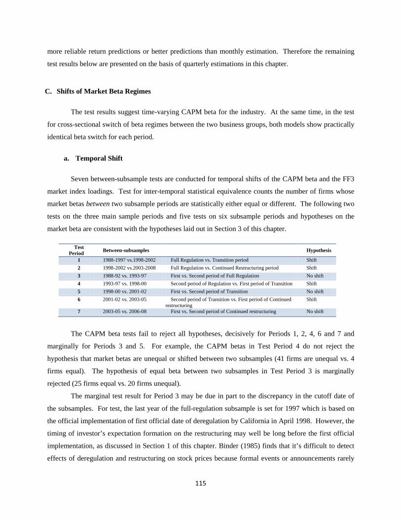
115

more reliable return predictions or better predictions than monthly estimation. Therefore the remaining

test results below are presented on the basis of quarterly estimations in this chapter.

C. Shifts of Market Beta Regimes

The test results suggest time-varying CAPM beta for the industry. At the same time, in the test

for cross-sectional switch of beta regimes between the two business groups, both models show practically

identical beta switch for each period.

a. Temporal Shift

Seven between-subsample tests are conducted for temporal shifts of the CAPM beta and the FF3

market index loadings. Test for inter-temporal statistical equivalence counts the number of firms whose

market betas between two subsample periods are statistically either equal or different. The following two

tests on the three main sample periods and five tests on six subsample periods and hypotheses on the

market beta are consistent with the hypotheses laid out in Section 3 of this chapter.

Test Period Between-subsamples Hypothesis

1 1988-1997 vs.1998-2002 Full Regulation vs. Transition period Shift 2 1998-2002 vs.2003-2008 Full Regulation vs. Continued Restructuring period Shift 3 1988-92 vs. 1993-97 First vs. Second period of Full Regulation No shift 4 1993-97 vs. 1998-00 Second period of Regulation vs. First period of Transition Shift 5 1998-00 vs. 2001-02 First vs. Second period of Transition No shift 6 2001-02 vs. 2003-05 Second period of Transition vs. First period of Continued

restructuring Shift

7 2003-05 vs. 2006-08 First vs. Second period of Continued restructuring No shift

The CAPM beta tests fail to reject all hypotheses, decisively for Periods 1, 2, 4, 6 and 7 and

marginally for Periods 3 and 5. For example, the CAPM betas in Test Period 4 do not reject the

hypothesis that market betas are unequal or shifted between two subsamples (41 firms are unequal vs. 4

firms equal). The hypothesis of equal beta between two subsamples in Test Period 3 is marginally

rejected (25 firms equal vs. 20 firms unequal).

The marginal test result for Period 3 may be due in part to the discrepancy in the cutoff date of

the subsamples. For test, the last year of the full-regulation subsample is set for 1997 which is based on

the official implementation of first official date of deregulation by California in April 1998. However, the

timing of investor’s expectation formation on the restructuring may well be long before the first official

implementation, as discussed in Section 1 of this chapter. Binder (1985) finds that it’s difficult to detect

effects of deregulation and restructuring on stock prices because formal events or announcements rarely

116

contain major new information. Binder finds no difference in information contents between monthly and

daily data and attributes it to investors’ anticipation of formal events or announcement.

Another marginal test result for Period 5 may be due also to a similar reason. The test period

covers two subsamples: the last few years of IT-led market boom and the first few years of bust. The two

subsamples may not be so homogenous or clear-cut in market risk or the CAPM beta. The high return

volatilities during the subsamples also may not be identical in nature, in scope, or in magnitude. Further

research is warranted.

In contrast, the FF3 market index loadings are statistically equal for all six between-subsample

tests, inconsistent with the return correlation test results. (Table 5-1) Furthermore, contrary to the

regulatory environment under full regulation, the FF beta estimates for the two subsamples of the full

regulation period reject the hypothesis of equal beta. Unlike the CAPM beta, the FF3 market betas more

or less remain stable inter-temporally and homogenous cross-sectionally. The relative invariance of the

FF3 market beta would reduce the information content of the market index loading and make it difficult

to make a unified measurement of systematic risk for stock returns. The shift of correlations largely

consistent with the economic, market, and industry conditions of the electric power industry suggest the

usefulness of information contents of return correlations as a measure of systematic risk.

An additional test on the Dow Jones Index firms conducted as a reference and for robustness

check offers additional insight. (Table 5-1) The FF3 market beta estimates for the DJ Index firms also

remain statistically equal for all seven test period. This test results are expected. The subsamples are

created based on the unique conditioning information for the restructuring process of the electric power

industry, a relatively homogeneous industry going through changes of an industry-wide policy and market

structure. On the other hand, the DJ Index firms are much more heterogeneous, comprised of a variety

industries and disparate products and services. Therefore when the same test is conducted on the DJ

Index firms on the same subsamples, the test results are expected neither to be as statistically strong as

those of the electric power industry nor to offer a clear economic story.

b. Cross-sectional Shifts

Six subsample tests are conducted for cross-sectional equivalence of the CAPM beta and the FF3

market index loadings between two business groups. Test for cross-sectional statistical equivalence

counts the number of quarters whose market betas between two business groups are statistically either

equal or different. The six subsample periods and hypotheses are consistent with the hypotheses laid out

in Section 4 of this chapter. The hypotheses posit that the market betas of two business groups were

117

homogeneous under full regulation (1988-1997), but diverged during the transition period and the

industry crisis (1998-2005), and then began to converge afterwards.

Subsample Test period Hypothesis

1988-92 p11 First period of Full regulation Equal

1993-97 p12 Second period of Full regulation Equal

1998-00 p21 First period of Transition Unequal

2001-02 p22 Second period of Transition Unequal

2003-05 p31 First period of Continuing Restructuring Unequal

2006-08 p32 Second period of Continuing Restructuring Equal

The test results of cross-sectional equivalence of beta estimates of the two business groups fail to

reject five hypotheses, but reject the hypothesis for 1998-2000. The test results of both models are

virtually identical, and the cross-sectional test results are statistically more significant than temporal shift.

(Table 5-2)

All beta estimates of two groups are statistically equal for the two subsample periods under full

regulation (p11, p12, or 1988-92, 1993-97). The statistical equality does not reject Hypothesis 1 on the

homogeneity of the two business group betas during regulation (1988-1997).

However, the test rejects Hypothesis 2-1 on the divergence of the two group betas at the

beginning period of restructuring (1998-2000). A plausible reason for the rejection is that, at the height of

the information technology boom, the new business opportunity of the electric power industry after

deregulation may have not been attractive enough to the investors compared to the perceived

opportunities in the “New Economy.” The opposite move of the stock prices of the industry in 1999 from

the general market during the height of the IT boom may corroborate the interpretation of the rejection of

the hypothesis.

The test does not reject Hypotheses 2-2 and 3 on the heterogeneity and inequality of two

businesses during the market and industry crises (2001-2002 and 2003-2005) and the hypothesis on the

convergence after the crisis (2003-2005). (Table 5-2)

As a robustness check, the same test is conducted on a randomly selected set of two businesses.

The test results decisively confirm the expected result of statistical equality of randomly selected

businesses for the CAPM beta and the FF3 model market index loadings. (Table 5-2) The test results on

the randomly selected samples corroborate the robustness of the test results on the electric power industry

firms, which largely substantiated the analysis on the economy, industry, and investment and financial

strategies of individual firms.

118

D. Structural Breaks

Tests for structural breakpoints using the CAPM beta estimates largely support the hypothesis for

a breakpoint in 2002 and another in 1998. On the other hand, the FF3 beta estimates pick the last end of

the test period and do not show any break for the rest of the entire test period.

Figure 4 counts the number of firms whose beta made structural break. The test method picks up

only one breakpoint for a test period. The test is conducted on three sample periods, the full period

(1988-2008), the period before the IT-led bubble bust and the electric power industry crisis (1988-2000),

and afterwards (2000-2008). The two subsamples overlap on the year 2000 to compensate for the five

percent truncation on both sides of subsamples.

For the entire test period (1988-2008), the test on the CAPM beta estimates indicates that a

structural break may have happened in July 2002. (Blue bars of Figure 4A) For the first period of

subsample, August 1998 is picked up, followed by October 1997 and May 1998. (Figure 4B) For the

second period of subsample, July 2002 is picked up again, followed by May 2002 and July 2001. (Figure

4C) On the other hand, when the FF3 model beta estimates are tested, the results are quite different. For

the entire test period (1988-2008), the test indicates that a structural break may have happened in the

second part of 2007 for the industry (Red bars of Figure 4A). For the first period of subsample, no

particular date is picked up. (Figure 4B) For the second period of subsample, the FF3 model picked April

2008. (Figure 4C)

Why are the results from the two models so different? As discussed earlier, the CAPM represents

the return correlations with the market and the relative volatilities more closely than the FF3 model does.

On the other hand, the FF3 model estimates are smoother than the CAPM as discussed earlier. The tests

have shown that return correlations and relative volatilities have made dramatic shifts through the

industry restructuring and through the IT-led market volatility. Therefore, the CAPM breakpoints appear

more realistic and plausible than the FF3 model. The 2007-2008 breakpoints of the FF3 model would

require longer data beyond the current test data for robustness.

6. Concluding Remarks

The best result from the tests in this chapter perhaps is a general confirmation of hypotheses on

stock return correlations, volatilities, market risks, model predictions, and breakpoints. The hypotheses

are formed, based on the conditioning information on the economy, the industry, the government policy,

and investment model and financing strategies of firms. The focused tests on individual firms provided

useful insight into the beta generating process, market risk, and regime switch of the market beta.

119

At the same time, the test results in this paper raise more questions than answers. Most questions

are primarily about “why?” and “how?” about the findings, although there must be many more yet-

undiscovered questions, “what has happened?” My future research will keep pursuing the discovered

questions through more in-depth investigations into firm-level returns, correlations, volatilities, factor

loadings, and model-predictions. The analytic scope of this paper stops short of a truly disaggregated

investigation.

Some more insight would be gained with the following additional research approaches. Financial

data need to be more formally and systematically related with stock return correlations, volatilities, and

the market risk than in this paper. Tests need to be conducted on expanded data such as other utility firms

or industries that had been restructured and deregulated in the past. (Cochrane, 2005; Lewellen et al.

2006)

120

Appendix

The Electric Power Industry Restructuring

The restructuring of the electric power industry offers additional experiment opportunities,

compared to other industries that had been restructured and became open to competition in the past

several decades.82 Unlike other restructured industries, not all sectors of the electric power market are

being opened to competition. While the electric power generation sector of the industry has become

increasingly open to competition, the transmission and distribution (T&D) sectors have remained

regulated and are expected to remain so because of the unique economic characteristics of the T&D

facilities as an infrastructure and the economies of scale. Therefore, individual firms have strategic

business choices. Some firms took on a competitive merchant business model and strategy for their

corporate investment and financing. Other firms chose to focus on the traditional, regulated electricity

utility model. As the competitive environment and policies have been evolving in a new experiment since

the 1990s, individual firms have continued to adjust their investment models and financing strategies. 83

Under the traditional regulation until California opened its electric power market to competition

in April 1998, an electric utility firm typically had been endowed with a monopolistic franchise privilege

to provide all electricity demand requirements in an exclusive service territory in exchange for practically

guaranteed returns on equity investment under the cost-plus pricing system. State regulators usually

allowed a return on equity of 10-12 percent and the industry had been among the most stable and safest

equity investment vehicles in the financial market.

The two distinct strategic investment models and financing strategies have emerged. The continued

evolution of restructuring over time provides a unique natural experiment to directly test for the changes

of market risk, inter-temporal and cross-sectional regime shifts of market betas across the firms.

A. Regulated Environment before 1998

84

82 The industries that had been restructured or deregulated since the 1970s include transportation (railroad, airlines, trucking), banking and financial services, telecommunications, and natural gas. 83 Under the restructuring and deregulation, electric power firms are allowed to control both business entities under certain rules for functional and financial separation; an electric power firm still operates both businesses as a legal entity and under the same common stock. This blend of businesses complicates analysis of pure competitive business vs. pure regulated business. Another complicating factor is that firms do not necessarily choose to or are allowed to transfer all power generation to competitive business; each firm has a different percentage of competitive business in its entire business. 84 The 1992-97 returns on equity (ROE) for the industry before the industry was open to competition were 10.7–12.1 percent. (Source: “2001 Financial Review,” by Edison Electric Institute)

The test period (1988-1997) under full regulation

had been punctuated by two policy events: the Energy Policy Act of 1992 (EPA of 1992) and the 1996

121

proceedings of the Federal Energy Regulatory Commission (FERC) that formally began to promote open

access to the transmission system and thrust state regulatory agencies into restructuring deliberations.85

What are the causes and consequences of the industry crisis? What implications do the

divergence of the electric power supply businesses and the industry crisis have on the betas? The high

expectations in the late 1990s on the new opportunities for competitive electric power supply business

resulted in an excess capacity of electric power supply by 2002, subsequently lowering expectations on

the future profitability amid cascading problems of high financial leverage, liquidity squeeze, credit rating

downgrades, dramatic stock price losses, corporate business and financial restructuring, fire-sale of assets,

divestitures of unprofitable business sectors, and bankruptcies of several merchant power firms. During

this time period, the economy and the general stock market also went through a serious downturn; the

U.S. stock market experienced bubble bursts in conjunction with the information technology. An

B. Transition into Deregulation and Competition, 1998-2002

The unique and dynamic events that took place during the transition period exposed the industry

and the firms to the risk of the market that happened to experience a “boom and bust.” During the

transition period for restructuring, the electric power industry went through two stock valuation cycles in

1999 and in 2001-2002, whereas the general market went through one “boom and bust” cycle. (Figure

A1-1) In April 1998, California became the first state to open the generation sector and wholesale power

markets of its electric power industry to competition; within the next few years, other 23 states and the

District of Columbia followed suit. In spite of high expectations of investors and managers about the new

opportunities for competitive electric power supply business, the industry stocks suffered negative returns

in 1999 as the general stock market continued to bring its high returns on the wave of the information

technology and “new economy” stocks. During the downturn of the second cycle of the industry stock

prices (2001-2002), the industry diverged. The stock prices of the regulated distribution business

continued relatively steady growth, while those of competitive merchant power supply business

experienced sharp losses, triggering a crisis for the industry.

85 A main objective of the EPA of 1992 was to open the electric power transmission system to potentially competitive suppliers such as non-utility entities, small electric power suppliers, and end-user as equally as to the transmission system owners and large electric power suppliers. The Act was a harbinger of the state-level restructuring and competition. In 1996, the FERC began a process to implement the “Open Access” to the transmission network system, the “essential facilities” in the industry. The open access paved a way to restructure the industry to competition. These policies of the federal government and the active deliberations of state governments in the 1990s to restructure the electric power market provided incentives for electric power firms earnestly to launch unregulated, competitive energy supply and service businesses in expectation of a restructured, competitive market.

122

economic recession followed.86

Unlike other industries that had been deregulated since the 1970s, not all sectors of the electric

power market will be deregulated. In a restructured market, the industry is separated into two main

sectors: the transmission and distribution (T&D) of electricity and the power generation and wholesale

marketing. The T&D sector will remain largely regulated as before. The transmission system is

regulated mainly by a federal agency, the Federal Energy Regulatory Commission (FERC); the

distribution system remains a natural monopoly regulated by state regulators in the traditional way. On

the other hand, the generation and wholesale marketing sector has been moving toward being increasingly

open to competition. Two major business strategies and investment models naturally have emerged: the

competitive merchant power generation and wholesale supply business, and the regulated, monopolistic

electric transmission and distribution business.

On the other hand, in 2000, the industry stocks rebounded strongly due in

part to high expectations on the restructuring and due in part to the general stock market declines which

began with the reversal of NASDAQ stocks in March 2000.

87 Unlike traditional utility firms, merchant power

suppliers generate wholesale electric power, market, and trade it in a competitive market; the suppliers are

fully exposed to a variety of market risks similar to firms in other competitive industries.88

In anticipation of deregulation, a majority number of firms chose the business model of higher

market risk by establishing unregulated, competitive merchant energy business during the second part of

Particularly

critical to merchant power business is the “spark spread,” the difference between wholesale electricity

prices (revenues) and natural gas prices (a major input factor cost). Firms of the second model will

remain fully regulated in transmission and retail distribution services with exclusive privileges to deliver

electricity to retail customers in a franchised territory.

86 Other major market disruptions also took place in 1998-2002, such as the financial fallouts of the Long-term Capital Management, the Asian and Russian currency and credit crises, the collapse of the communistic political and economic system and the subsequent world political turmoil and economic recession, the terrorist attacks and political unrest, and the celebrated revelation of accounting frauds. 87 Almost all firms have certain portions of both competitive merchant business and regulated utility business. Firms that heavily moved toward competitive merchant business generally declared their business investment model as such and pursued aggressive merchant generating power plant development and heavy debt financing. On the other hand, some firms that pursued unregulated but non-generating businesses were spared from a dramatic stock price declines during the industry crisis in 2001-2002. 88 This paper focuses on the investor-owned electric utility firms and non-utility power producers which provide approximately 75 percent of electricity in the U.S. Non-utility power producers include independent power companies, merchant generators, and power marketers. Not included in the analysis of this paper are three other electric power generation or distribution entities: Federal government-owned and -operated electric power agencies such as Tennessee Valley Authority and Bonneville Power Authority, approximately 1,850 municipal government utilities, and approximately 900 electric rural cooperatives. Most of municipal and cooperative utilities are engaged in the electric power distribution to retail customers in their franchised service territories and are expected to remain largely regulated by state and local governments. Included in the cooperatives are electric generation and transmission (G&T) cooperatives which generate electricity for their distribution cooperative members/owners.

123

the 1990s and pushed aggressive investment in electric power generation facilities, energy trading

operations, and other related businesses to secure first-mover advantage with heavy debt financing. 89

Investors also supplied low-cost credit and pushed high stock prices of such firms in the 1990s. As firms

aggressively pushed competitive businesses in electric power generation, wholesale marketing, and other

businesses, the electric power market became oversupplied, and the competitive generation and wholesale

power market collapsed in 2001 over concerns about the expected narrowing or even a negative spark

spread, high financial leverages, and the liquidity issues. (Figures A1-2 and A1-3) Ironically the

California market exploded due to high wholesale electricity prices in 2000-01 amid a concern about

oversupply in the nation.90

Firms that aggressively invested with external financing now faced serious liquidity problems and

defaults in 2002, and began to redirect their corporate investment strategies, financial structure, and

operational priorities, except for a few firms that had exited from or reduced volatile and unprofitable

trading business before 2000. During full regulation, the stable, predictable, and conservative investment

and financing helped firm even improve financial structure and the interest coverage ratio

Under a deregulation rule, electric power firms must pay whole power

purchase prices to the Power Exchange without being able to transfer the cost higher than the agreed-upon

retail prices to the consumers. California suspended its deregulation in April 2001 and other states that

were moving toward deregulation withheld or cancelled the restructuring process.

Under full regulation through 1998, utility firms had invested approximately three quarters of

cash flows from operation (CFO), or the investment ratio to CFO even declined somewhat during the first

part of the 1990s. Net financing was a negative quarter of CFO, which indicates that overall utility firms

had no net external financing and firms spent the remaining quarter of CFO for dividend payout and debt

payment. However, firms began to aggressively invest with external financing with the opening of the

power generation sector to competition. In 1999-2002, firms invested up to two times the CFO, which is

financed with external debt up to the matching amount of CFO. (Figures A2-1 through A2-3) Firms that

pursued competitive merchant business were more aggressive in investment and external financing; the

utility firms that are grouped into regulated business in this study also attempted to diversify into

competitive energy and non-energy business albeit less aggressively and within narrower scopes of

businesses. The aggressive investment resulted in oversupply and lowered the expected power prices and

profits.

89 Other businesses firms pursued included electric businesses in foreign lands, telecommunications, the Internet service provider, real estate development, automobile auctions. 90 A confluence of factors contributed to the California market “meltdown” in 2000-01. The factors included faulty deregulation policy, unusual weather and mechanical failures, and wholesale electric and natural gas price manipulations by energy traders. (FERC, 2003)

124

(EBITDA/interest payment), the former is a critical indicator of long-term solvency, the latter an indicator

of short-term liquidity. (Figure A2-4) However, during the transition period, firms dramatically

increased financial leverage almost up to 70 percent from 50-55 percent under regulation, while the short-

term liquidity deteriorated down to two times in 2002 from a high of five times during regulation. (Figure

A2-3) These risky trends are natural consequences of the aggressive investment and external financing

firms pursued during the transition period. The liquidity and solvency risk of the firms that pursued

competitive merchant business deteriorated faster and deeper, as a mirror image of the aggressive

investment and ambitious external financing.91

Then, the electric power supply in California was disrupted in 2000-01; the defects in the

restructuring became clear, and fraudulent accounting practices and electric power trading irregularities

were exposed.

92

The sharp stock price drop-offs during the industry crisis took place between the end of 2001 and

the early 20003. The “fiasco” of the California electric power market in 2000-2001 and the celebrated

revelation and scandal of energy trading and accounting frauds of Enron and other merchant power

business firms in 2001-2002 added salt to the wounds of oversupply and lower profit expectation. In

2002-2003, 41 out of 51 electric power firms experienced sharp drops in stock prices from the highest

loss of 99.1 percent to the lowest loss of 21.9 percent. On the other hand, 10 firms experienced stock

price gains during the period. The gains also were similarly dramatic from the highest gain of 87.5

percent to the lowest gain of 37.6 percent. All firms that aggressively pursued competitive merchant

business are among the top losers of stock prices. (For additional discussion, refer to Section 3 and Table

1 in the Appendix to Chapter 3) All firms that experienced stock price gains during the industry crisis

above had adopted the regulated distribution business. Firms that adopted a varying mix of both

businesses fell in between and suffered a varying degree of losses, but still a significant minimum of 21.9

percent. Some firms originally had adopted aggressive competitive merchant power supply business

models and financing strategies including proprietary speculative energy trading business in mid-1990s.

In addition, as the aggressive investment in electricity generation plants by firms

resulted in overcapacity, the expected profitability of the merchant power business became bleak. Debts

that had been piled up by firms to finance investment triggered a shower of credit rating downgrades and

stock price drops.

93

91 For additional discussion, refer to Section 2 of this chapter and relevant data. 92 For detailed investigation report, refer to the “Final Report on Price Manipulation In Western Markets“ by FERC (March 2003) This report also helps understand the defective deregulation rules that incentivized trading frauds.

93 However, those firms soon observed that everyone was jumping on the wagon and realized that an oversupply of electric power was going to soon ensue and the profit margins of trading business were going to narrow thin. The

125

In the meantime, in August 2005, U.S. Congress enacted the Energy Policy Act (EPA of 2005) to

promote reliable and competitive power supply through a nationwide network infrastructure development

of electric power transmission system. The Act reinforced the authority and expanded the responsibility

of the Federal Energy Regulatory Commission (FERC) on the development of, and open access to, the

transmission infrastructure. Because the Act empowered the FERC with a nearly full authority over

transmission network systems, the transmission network systems has become increasingly regulated by

the FERC, while the ownership of the systems remains retained by private owners or electric power firms.

C. A Measured Move toward Restructuring after the “fiasco”

During the third period (2003-2006), many firms restored the financial strengths and went “back-

to-basic” to their “core” businesses. Firms divested themselves of competitive or “non-core” businesses

and went back to the “integrated utility or energy business,” while keeping the door open to future

competitive merchant business opportunities. The State of Virginia reversed deregulation in January

2007 and began to re-regulate the industry. On the other hand, the electric power generation and

wholesale market sector has been slowly but steadily moving toward full deregulation and competition,

particularly since the Congress enacted the EPA in August 2005 and opened wide the door to business

combinations among electric power firms and also to the entry of non-energy business entities into

electricity business.94

firms refrained themselves from additional risky investment and remained relatively unscathed. Examples include Entergy in Louisiana, Dominion Resources in Virginia, and Excelon Energy in Illinois.

94 The repeal of the decades-old Public Utility Holding Company Act (PUHCA) of 1935 by the EPA of 2005 significantly removed the entry and merger barriers. As a result, acquisitions of electric power business by non-utility firms have sharply increased in the next few years of the EPA of 2005.

126

Figure A1-1 Stock Prices

Figure A1-2

New Capacity Installations

Figure A1-3

Stock Prices (daily) excluding data series with missing data

0

200

400

600

800

1000

1200

1400

1600

1986

1986

1987

1987

1988

1988

1989

1989

1990

1990

1991

1991

1992

1992

1993

1993

1994

1994

1995

1995

1996

1996

1997

1997

1998

1998

1999

1999

2000

2000

2001

2001

2002

2002

2003

2003

2004

2004

2005

2005

2006

2006

Merchant Pow er Firms Traditional Regulated Firms S&P500

Capacity Margin

12

13

14

15

16

17

18

19

20

21

22

1993 1994 1995 1996 1997 1998 1999 2000 2001 2002 2003 2004

%

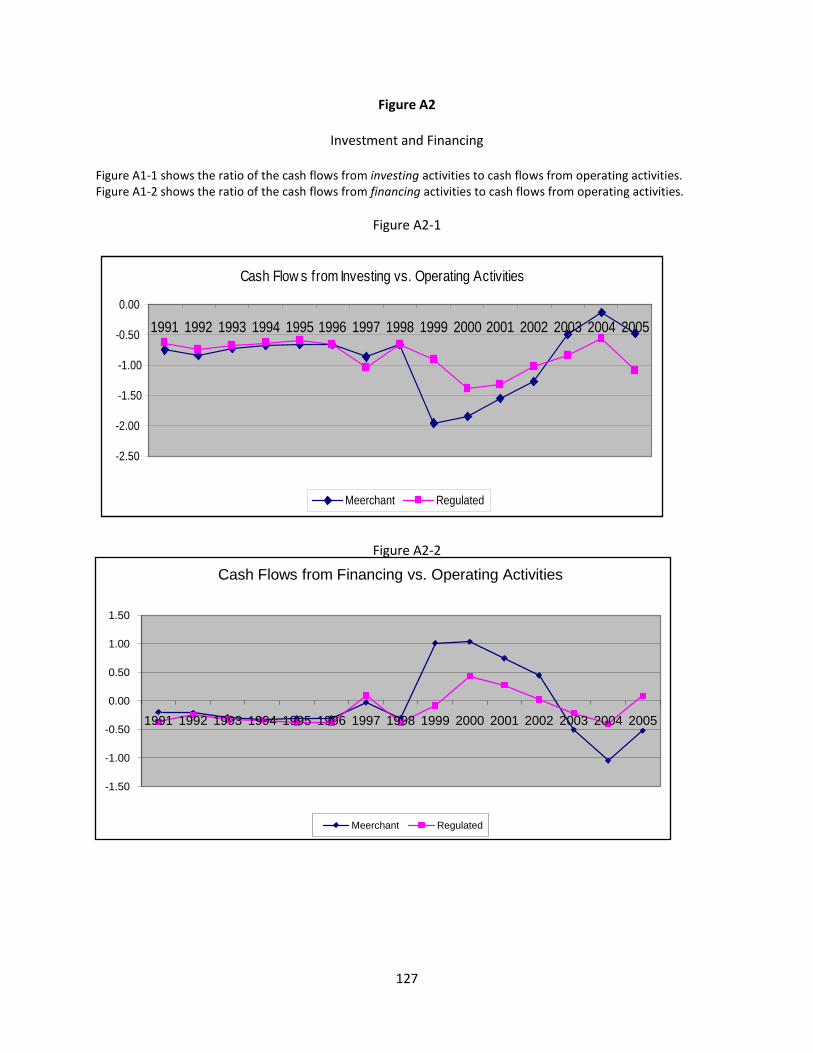
127

Figure A2

Investment and Financing Figure A1-1 shows the ratio of the cash flows from investing activities to cash flows from operating activities. Figure A1-2 shows the ratio of the cash flows from financing activities to cash flows from operating activities.

Figure A2-1

Figure A2-2

Cash Flow s from Investing vs. Operating Activities

-2.50

-2.00

-1.50

-1.00

-0.50

0.00

1991 1992 1993 1994 1995 1996 1997 1998 1999 2000 2001 2002 2003 2004 2005

Meerchant Regulated

-1.50

-1.00

-0.50

0.00

0.50

1.00

1.50

1991 1992 1993 1994 1995 1996 1997 1998 1999 2000 2001 2002 2003 2004 2005

Cash Flows from Financing vs. Operating Activities

Meerchant Regulated

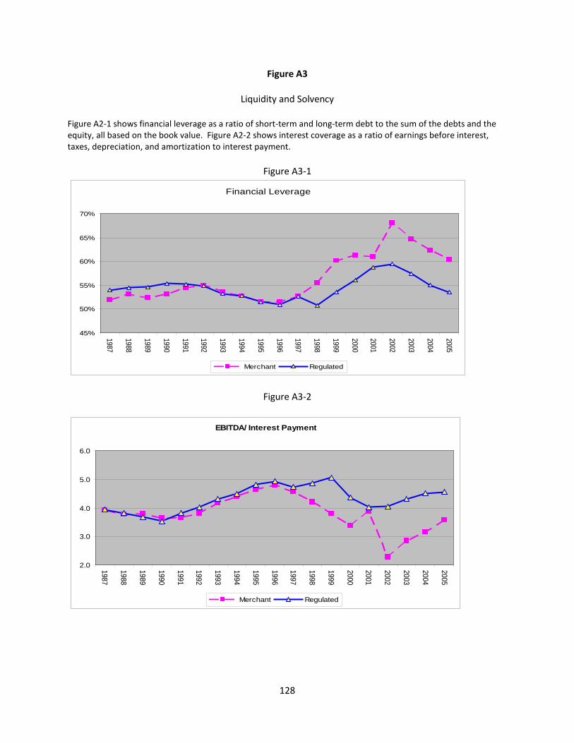
128

Figure A3

Liquidity and Solvency Figure A2-1 shows financial leverage as a ratio of short-term and long-term debt to the sum of the debts and the equity, all based on the book value. Figure A2-2 shows interest coverage as a ratio of earnings before interest, taxes, depreciation, and amortization to interest payment.

Figure A3-1

Figure A3-2

Financial Leverage

45%

50%

55%

60%

65%

70%

1987

1988

1989

1990

1991

1992

1993

1994

1995

1996

1997

1998

1999

2000

2001

2002

2003

2004

2005

Merchant Regulated

EBITDA/ Interest Payment

2.0

3.0

4.0

5.0

6.0

1987

1988

1989

1990

1991

1992

1993

1994

1995

1996

1997

1998

1999

2000

2001

2002

2003

2004

2005

Merchant Regulated

129

References for Chapter 3

Averch Harve and Leland L. Johnson, “Behavior of the Firm under Regulatory Constraint,” The American Economic Review, December 10962

Binder, John J., ”Measuring the Effects of regulation with stock price data,” Rand Journal of Economics, Summer, 1985

Blume, Marshall, “Beta and their Regression Tendencies: Some further evidence,” The Journal of Finance, March 1979

Blume, Marshall, “Beta and their Regression Tendencies” The Journal of Finance, March 1975

Blume, Marshall, “On the Assessment of Risk,” The Journal of Finance, March 1971

Braun, Maias and Borja Larrain, “Finance and the Business Cycle: International, Inter-Industry Evidence,” The Journal of Finance, 2004

Braun, Phillip, Daniel B. Nelson, and Alain M. Sunier, “Good News, Bad News, Volatility, and Betas,” The Journal of Finance, Vol., L, No. 5, December 1995

Breen, William J. and Eugene M. Lerner, “On the use of beta in regulatory proceedings,” The Bell Journal of Economics, 1972

Chen, Nai Fu, Richard Roll, and Stephen A. Ross, “Economic Forces and the Stock Market” Journal of Business, 1986 Chen, Son-nan, “Beta non-stationarity, Portfolio residual risk and Diversification,” Journal of Financial and Quantitative Analysis, March 1981 Clarke, Roger G., “The Effect of Fuel Adjustment Clause on the Systematic Risk and Market Value of Electric Utilities,” The Journal of Finance, 1980

Comin, Diego and Thomas Phillippon, “The Rise in Firm-level volatility: Causes and Consequences,” NBER working paper 11388, May 2005

DeJong, Douglas V. and Daniel W. Collins, “Explanations for the Instability of Equity Beta: Risk-free rates changes and Leverage Effects,” Journal of Financial and Quantitative Analysis, March 1985

Fama, Eugene G. and K. French, “Industry Costs of Equity,” Journal of Financial Economics, 1997 Fama, Eugene G. and K. French, “Common risk factors in the returns on stocks and bonds,” Journal of Financial Economics, 1993 Gooding, Arthur E. and Terence P. O’Malley, “Market Phase and the Stationarity of of Beta,” Journal of Financial and Quantitative Analysis, December 1977 Grout and Zalewska, “The impact of regulation on market risk,” Journal of Financial Economics, 2006 Hamada, Robert S., “The Effect of the Firm’s Capital Structure on the systematic Risk of Common Stocks,” Journal of Finance 1972

130

Hays, Patrick A. and David E. Upton, “A shifting Regimes Approach to the Stationarity of the market Model Parameters of Individual Securities,” Journal of Financial and Quantitative Analysis, September 1986 Horwitz, Robert B., “Understanding deregulation,” Theory and Society, 1986 Lewellen, Jonathan, Stefan Nagel, and Jay Shanken, “A Skeptical Appraisal of Asset Pricing Tests,” Journal of Financial Economics, 2006 Melcher, Ronald W., “Financial Factors which influence Beta variations within an Homogeneous industry environment,” Journal of financial and Quantitative analysis, March 1974 Miller, Merton H. and Franco Modigliani, “Some Estimates of the Cost of Capital to the Electric Utility Industry, 1954-1957, The American Economic Review, June 1966 Norton, Seth W., “Regulation and Systematic Risk: the case of electric utilities,” The Journal of Law and Economics, 1985 Rozenzweig, Mark R. and Kenneth I. Wolpin, Natural “Natural Experiments” in Economics. Journal of Economic Literature

Robichek, Alexander A., Robert C. Higgins, and Michael Kinsman, “The Effect of Leverage on the Cost of Equity Capital of Electric Utility Firms,” The Journal of Finance, May 1973

Theobald, Michael, “Beta Stationarity and Estimation Period,” Journal of Financial and Quantitative Analysis,,December 1981

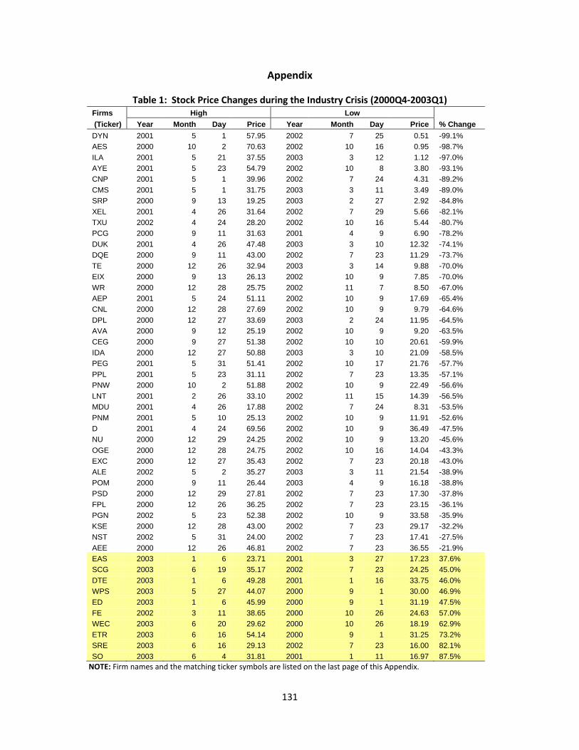
131

Appendix

Table 1: Stock Price Changes during the Industry Crisis (2000Q4-2003Q1) Firms High Low

% Change (Ticker) Year Month Day Price Year Month Day Price DYN 2001 5 1 57.95 2002 7 25 0.51 -99.1% AES 2000 10 2 70.63 2002 10 16 0.95 -98.7% ILA 2001 5 21 37.55 2003 3 12 1.12 -97.0% AYE 2001 5 23 54.79 2002 10 8 3.80 -93.1% CNP 2001 5 1 39.96 2002 7 24 4.31 -89.2% CMS 2001 5 1 31.75 2003 3 11 3.49 -89.0% SRP 2000 9 13 19.25 2003 2 27 2.92 -84.8% XEL 2001 4 26 31.64 2002 7 29 5.66 -82.1% TXU 2002 4 24 28.20 2002 10 16 5.44 -80.7% PCG 2000 9 11 31.63 2001 4 9 6.90 -78.2% DUK 2001 4 26 47.48 2003 3 10 12.32 -74.1% DQE 2000 9 11 43.00 2002 7 23 11.29 -73.7% TE 2000 12 26 32.94 2003 3 14 9.88 -70.0% EIX 2000 9 13 26.13 2002 10 9 7.85 -70.0% WR 2000 12 28 25.75 2002 11 7 8.50 -67.0% AEP 2001 5 24 51.11 2002 10 9 17.69 -65.4% CNL 2000 12 28 27.69 2002 10 9 9.79 -64.6% DPL 2000 12 27 33.69 2003 2 24 11.95 -64.5% AVA 2000 9 12 25.19 2002 10 9 9.20 -63.5% CEG 2000 9 27 51.38 2002 10 10 20.61 -59.9% IDA 2000 12 27 50.88 2003 3 10 21.09 -58.5% PEG 2001 5 31 51.41 2002 10 17 21.76 -57.7% PPL 2001 5 23 31.11 2002 7 23 13.35 -57.1% PNW 2000 10 2 51.88 2002 10 9 22.49 -56.6% LNT 2001 2 26 33.10 2002 11 15 14.39 -56.5% MDU 2001 4 26 17.88 2002 7 24 8.31 -53.5% PNM 2001 5 10 25.13 2002 10 9 11.91 -52.6% D 2001 4 24 69.56 2002 10 9 36.49 -47.5% NU 2000 12 29 24.25 2002 10 9 13.20 -45.6% OGE 2000 12 28 24.75 2002 10 16 14.04 -43.3% EXC 2000 12 27 35.43 2002 7 23 20.18 -43.0% ALE 2002 5 2 35.27 2003 3 11 21.54 -38.9% POM 2000 9 11 26.44 2003 4 9 16.18 -38.8% PSD 2000 12 29 27.81 2002 7 23 17.30 -37.8% FPL 2000 12 26 36.25 2002 7 23 23.15 -36.1% PGN 2002 5 23 52.38 2002 10 9 33.58 -35.9% KSE 2000 12 28 43.00 2002 7 23 29.17 -32.2% NST 2002 5 31 24.00 2002 7 23 17.41 -27.5% AEE 2000 12 26 46.81 2002 7 23 36.55 -21.9% EAS 2003 1 6 23.71 2001 3 27 17.23 37.6% SCG 2003 6 19 35.17 2002 7 23 24.25 45.0% DTE 2003 1 6 49.28 2001 1 16 33.75 46.0% WPS 2003 5 27 44.07 2000 9 1 30.00 46.9% ED 2003 1 6 45.99 2000 9 1 31.19 47.5% FE 2002 3 11 38.65 2000 10 26 24.63 57.0% WEC 2003 6 20 29.62 2000 10 26 18.19 62.9% ETR 2003 6 16 54.14 2000 9 1 31.25 73.2% SRE 2003 6 16 29.13 2002 7 23 16.00 82.1% SO 2003 6 4 31.81 2001 1 11 16.97 87.5%

NOTE: Firm names and the matching ticker symbols are listed on the last page of this Appendix.

132

Table 2 Model Specification and Parameter Estimates

The “X” marks represent statistically significant factor loadings in the FF3 model. The “% of significant regressions” represents the number of regressions where a factor loading is statistically significant by itself or in combination with other significant factor loadings, provided that the alpha is insignificant. Any factor loading with significant alphas are excluded in Specifications 1 through 8.

Specification Market Index

SMB HML Quarterly estimation Annual estimation

Count % Count %

1 x 913 0.283 108 0.115

2 x x 224 0.070 79 0.084

3 x x x 178 0.055 292 0.310 4 x x 983 0.305 416 0.442 5 x x 30 0.009

6 x 106 0.033 3 0.003

7 x 70 0.022

8 ALL three risk variables are insignificant 553 0.172 15 0.016 9 Alpha is significant 166 0.052 29 0.031

Total 3223 1.000 942 1.000

% of significant regressions

Annual estimation

0.950 0.397 0.752

Quarterly estimation

0.713 0.167 0.391

133

Table 3 Number of Significant Betas and Insignificant Alphas:

Annual and Quarterly Estimations (CAPM vs. FF3 Model)

Each number represents the number of regressions where the CAPM beta, the FF3 model market index loading, or alpha estimate is statistically significant or insignificant. Each model should add up to 45 for annual regressions, and 180 for quarterly regressions. Annual Estimation Quarterly estimation Beta significant insignificant significant insignificant Alpha insignificant significant insignificant significant insignificant significant insignificant significant Model CAPM FF3 CAPM FF3 CAPM FF3 CAPM FF3 CAPM FF3 CAPM FF3 CAPM FF3 CAPM FF3 1991 43 39 2 6 133 105 9 7 36 62 2 6 1992 38 38 7 7 94 76 3 4 82 97 1 3 1993 44 45 1 130 144 4 41 35 5 1 1994 44 44 1 1 155 146 2 13 23 21 1995 40 44 1 1 4 96 70 78 107 6 3 1996 43 40 1 5 1 152 143 2 6 25 30 1 1 1997 39 42 5 1 1 2 128 107 20 11 23 55 9 7 1998 36 43 1 1 7 1 1 75 105 1 7 102 66 2 2 1999 31 44 11 3 1 68 64 9 4 87 98 16 14 2000 6 45 3 30 6 18 130 1 8 140 41 21 1 2001 27 45 18 66 126 2 5 111 48 1 1 2002 45 45 142 149 2 2 34 25 2 4 2003 44 44 1 1 162 161 1 2 16 17 1 2004 43 44 2 1 164 154 3 2 13 24 2005 44 45 1 160 167 20 13 2006 42 44 2 1 1 135 159 11 3 32 18 2 2007 45 43 2 149 144 24 27 4 6 2008 41 41 1 1 151 148 9 8 6 10 Total 823 895 36 28 76 18 7 1 2178 2298 123 122 853 760 69 43

% 0.874 0.950 0.038 0.030 0.081 0.019 0.007 0.001 0.676 0.713 0.038 0.038 0.265 0.236 0.021 0.013

134

Table 4 Correlations between

Model-predicted stock returns and Realized returns

This Table shows the correlations between the model-predicted stock returns and the realized returns for the full period (1988-2008) and three subsample periods (1988-1997,1998-2002,and 2003-2008). The model-predicted stock returns are based on Equation 3 in Chapter 1:

CAPM: E(ri – rf) = E[ b i (rm – rf) ] FF3 Model: E(ri – rf) = E[ b i,1*(rm – rf) + b i,2*SMBi + b i,3*HMLi]

Frequency Percentage Correlation Coefficients

positive negative positive negative positive negative CAPM FF3 CAPM FF3 CAPM FF3 CAPM FF3 CAPM FF3 CAPM FF3

Significant

Annual

1988-2008 30 40 0.667 0.889 0.558 0.639

1988-1997 25 11 0.556 0.244 0.764 0.736

1998-2002 16 0.356 0.929

2003-2008 24 27 0.533 0.600 0.907 0.896

Quarterly

1988-2008 41 43 0.911 0.956 0.375 0.455

1988-1997 37 37 0.822 0.822 0.414 0.422

1998-2002 13 29 0.289 0.644 0.522 0.559

2003-2008 20 31 0.444 0.689 0.523 0.581

Monthly

1988-2008 44 44 0.978 0.978 0.300 0.366

1988-1997 40 39 0.889 0.867 0.298 0.381

1998-2002 21 38 1 0.467 0.844 0.022 0.373 0.440 -0.256

2003-2008 44 40 0.978 0.889 0.397 0.407

Insignificant

annual

1988-2008 15 5 0.333 0.111 0.296 0.314

1988-1997 20 33 1 0.444 0.733 0.022 0.491 0.419 -0.138

1998-2002 23 27 22 2 0.511 0.600 0.489 0.044 0.381 0.617 -0.279 -0.305

2003-2008 19 16 2 2 0.422 0.356 0.044 0.044 0.615 0.660 -0.217 -0.225

quarterly

1988-2008 4 2 0.089 0.044 0.123 0.104

1988-1997 7 7 1 1 0.156 0.156 0.022 0.022 0.236 0.235 -0.030 -0.028

1998-2002 30 15 2 1 0.667 0.333 0.044 0.022 0.232 0.291 -0.204 -0.140

2003-2008 24 13 1 1 0.533 0.289 0.022 0.022 0.292 0.276 -0.035 -0.105

monthly

1988-2008 1 1 0.022 0.022 0.098 -0.096

1988-1997 3 6 2 0.067 0.133 0.044 0.163 0.129 -0.017

1998-2002 22 4 1 3 0.489 0.089 0.022 0.067 0.171 0.173 -0.040 -0.084

2003-2008 1 5 0.022 0.111 0.015 0.122

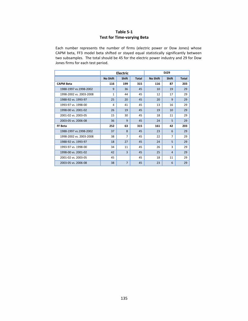
135

Table 5-1 Test for Time-varying Beta

Each number represents the number of firms (electric power or Dow Jones) whose CAPM beta, FF3 model beta shifted or stayed equal statistically significantly between two subsamples. The total should be 45 for the electric power industry and 29 for Dow Jones firms for each test period. Electric DJ29

No Shift Shift Total No Shift Shift Total

CAPM Beta 116 199 315 116 87 203

1988-1997 vs.1998-2002 9 36 45 10 19 29

1998-2002 vs. 2003-2008 1 44 45 12 17 29

1988-92 vs. 1993-97 25 20 45 20 9 29

1993-97 vs. 1998-00 4 41 45 13 16 29

1998-00 vs. 2001-02 26 19 45 19 10 29

2001-02 vs. 2003-05 15 30 45 18 11 29

2003-05 vs. 2006-08 36 9 45 24 5 29

FF Beta 252 63 315 161 42 203

1988-1997 vs.1998-2002 37 8 45 23 6 29

1998-2002 vs. 2003-2008 38 7 45 22 7 29

1988-92 vs. 1993-97 18 27 45 24 5 29

1993-97 vs. 1998-00 34 11 45 26 3 29

1998-00 vs. 2001-02 42 3 45 25 4 29

2001-02 vs. 2003-05 45 45 18 11 29

2003-05 vs. 2006-08 38 7 45 23 6 29

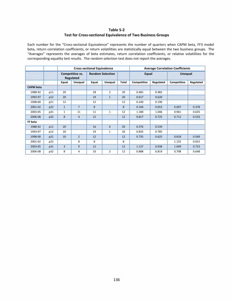
136

Table 5-2 Test for Cross-sectional Equivalence of Two Business Groups

Each number for the “Cross-sectional Equivalence” represents the number of quarters when CAPM beta, FF3 model beta, return correlation coefficients, or return volatilities are statistically equal between the two business groups. The “Averages” represents the averages of beta estimates, return correlation coefficients, or relative volatilities for the corresponding equality test results. The random selection test does not report the averages.

Cross-sectional Equivalence Average Correlation Coefficients

Competitive vs. Regulated

Random Selection Equal Unequal

Equal Unequal Equal Unequal Total Competitive Regulated Competitive Regulated

CAPM beta

1988-92 p11 20 18 2 20 0.482 0.482

1993-97 p12 20 19 1 20 0.617 0.620

1998-00 p21 12 12 12 0.240 0.190

2001-02 p22 1 7 8 8 0.104 0.053 0.697 0.378

2003-05 p31 1 11 11 1 12 1.180 1.046 0.961 0.635

2006-08 p32 8 4 12 12 0.817 0.725 0.712 0.533

FF beta

1988-92 p11 20 16 4 20 0.576 0.539

1993-97 p12 20 19 1 20 0.835 0.785

1998-00 p21 10 2 12 12 0.735 0.625 0.818 0.569

2001-02 p22 8 8 8 1.155 0.652

2003-05 p31 3 9 12 12 1.127 0.938 1.049 0.723

2006-08 p32 8 4 10 2 12 0.888 0.819 0.798 0.648

137

Figure 1 Stock Price Changes

This figure matches with Table 1 that shows stock price changes of electric power firms during the industry crisis.

1-B. Stock Prices

The prices of the two electric power stock groups are equal-weighted aggregates of individual firm stock prices. A few new electric power firms with partial data are also included. The competitive and merchant power business is represented in blue color; the traditional, regulated utility business in red color.

-100%

-80%

-60%

-40%

-20%

0%

20%

40%

60%

80%

100%D

YN AES ILA

AYE

CNP

CMS

SRP

XEL

TXU

PCG

DU

KD

QE TE EIX

WR

AEP

CNL

DPL

AV

ACE

GID

APE

GPP

LPN

WLN

TM

DU

PNM D

NU

OG

EEX

CA

LEPO

MPS

DFP

LPG

NKS

EN

STA

EE EAS

SCG

DTE

WPS ED FE

WEC ET

RSR

ESO

1-A. Stock price changes(2000.q4-2003.q1)

Stock Prices (daily) excluding data series with missing data

0

200

400

600

800

1000

1200

1400

1600

1986

1986

1987

1987

1988

1988

1989

1989

1990

1990

1991

1991

1992

1992

1993

1993

1994

1994

1995

1995

1996

1996

1997

1997

1998

1998

1999

1999

2000

2000

2001

2001

2002

2002

2003

2003

2004

2004

2005

2005

2006

2006

Merchant Pow er Firms Traditional Regulated Firms S&P500

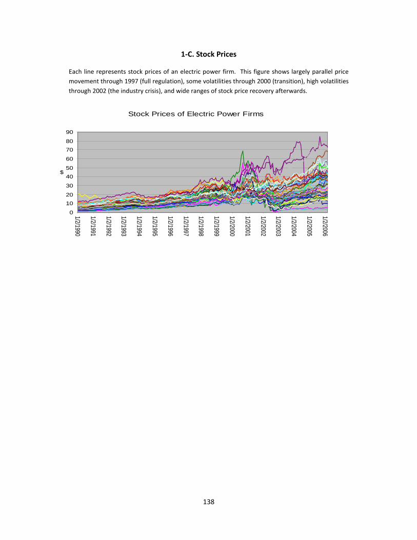
138

1-C. Stock Prices

Each line represents stock prices of an electric power firm. This figure shows largely parallel price movement through 1997 (full regulation), some volatilities through 2000 (transition), high volatilities through 2002 (the industry crisis), and wide ranges of stock price recovery afterwards.

Stock Prices of Electric Power Firms

0

1020

30

4050

60

7080

90

1/2/1990

1/2/1991

1/2/1992

1/2/1993

1/2/1994

1/2/1995

1/2/1996

1/2/1997

1/2/1998

1/2/1999

1/2/2000

1/2/2001

1/2/2002

1/2/2003

1/2/2004

1/2/2005

1/2/2006

$

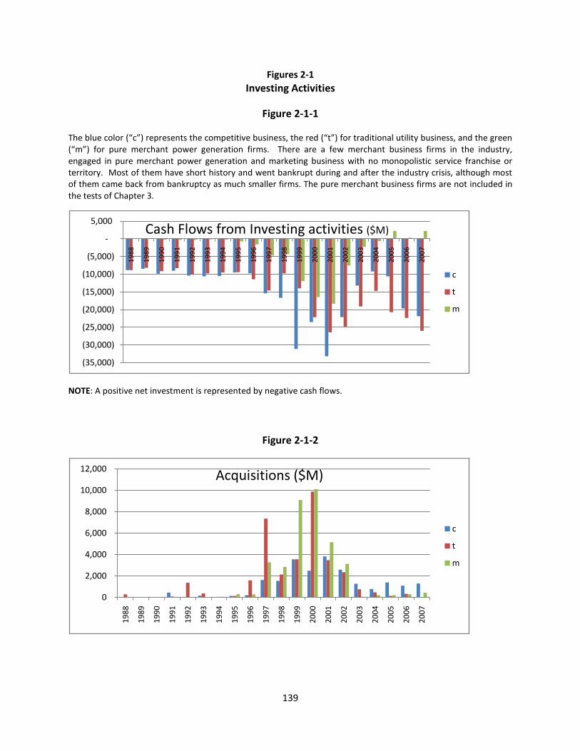
139

Figures 2-1 Investing Activities

Figure 2-1-1

The blue color (“c”) represents the competitive business, the red (“t”) for traditional utility business, and the green (“m”) for pure merchant power generation firms. There are a few merchant business firms in the industry, engaged in pure merchant power generation and marketing business with no monopolistic service franchise or territory. Most of them have short history and went bankrupt during and after the industry crisis, although most of them came back from bankruptcy as much smaller firms. The pure merchant business firms are not included in the tests of Chapter 3.

NOTE: A positive net investment is represented by negative cash flows.

Figure 2-1-2

(35,000)

(30,000)

(25,000)

(20,000)

(15,000)

(10,000)

(5,000)

-

5,000

1988

1989

1990

1991

1992

1993

1994

1995

1996

1997

1998

1999

2000

2001

2002

2003

2004

2005

2006

2007

Cash Flows from Investing activities ($M)

c

t

m

0

2,000

4,000

6,000

8,000

10,000

12,000

1988

1989

1990

1991

1992

1993

1994

1995

1996

1997

1998

1999

2000

2001

2002

2003

2004

2005

2006

2007

Acquisitions ($M)

c

t

m

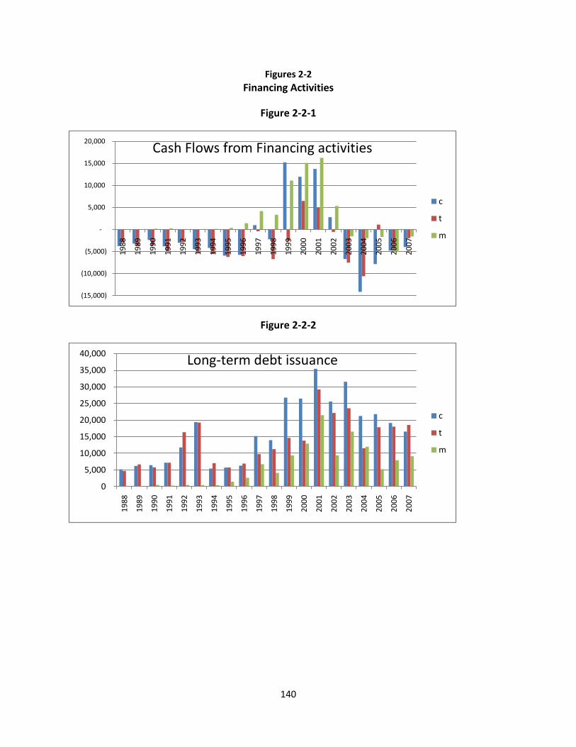
140

Figures 2-2 Financing Activities

Figure 2-2-1

Figure 2-2-2

(15,000)

(10,000)

(5,000)

-

5,000

10,000

15,000

20,000

1988

1989

1990

1991

1992

1993

1994

1995

1996

1997

1998

1999

2000

2001

2002

2003

2004

2005

2006

2007

Cash Flows from Financing activities

c

t

m

0

5,000

10,000

15,000

20,000

25,000

30,000

35,000

40,000

1988

1989

1990

1991

1992

1993

1994

1995

1996

1997

1998

1999

2000

2001

2002

2003

2004

2005

2006

2007

Long-term debt issuance

c

t

m

141

Figure 2-2-3

Figure 2-2-4

-

20,000

40,000

60,000

80,000

100,000

120,000

140,000

1988

1989

1990

1991

1992

1993

1994

1995

1996

1997

1998

1999

2000

2001

2002

2003

2004

2005

2006

2007

Total Long-term debt

c

t

m

0

5,000

10,000

15,000

20,000

25,000

1988

1989

1990

1991

1992

1993

1994

1995

1996

1997

1998

1999

2000

2001

2002

2003

2004

2005

2006

2007

Long-term debt due

c

t

m

142

Figure 2-3 Net Income and Operating Cash Flows

Figure 2-3-1

Figure 2-3-2

(15,000)

(10,000)

(5,000)

0

5,000

10,000

15,000

20,000

1988

1989

1990

1991

1992

1993

1994

1995

1996

1997

1998

1999

2000

2001

2002

2003

2004

2005

2006

2007

Net income

c

t

m

0

5,000

10,000

15,000

20,000

25,000

30,000

1988

1989

1990

1991

1992

1993

1994

1995

1996

1997

1998

1999

2000

2001

2002

2003

2004

2005

2006

2007

Cash Flows from Operating activities

c

t

m

143

Figure 3-1-1

Two model results are compared: the CAPM and the FF3 model

Figure 3-1-2

-0.002

-0.001

0

0.001

0.002

0.003

0.004

0.005

1988

1990

1992

1994

1996

1998

2000

2002

2004

2006

2008

1989

1991

1993

1995

1997

1999

2001

2003

2005

2007

capm ff

Alpha Estimates (quarterly)

c - Average of c c - StdDev of c t - Average of c t - StdDev of c

0

0.2

0.4

0.6

0.8

1

1.2

1.4

1988

1990

1992

1994

1996

1998

2000

2002

2004

2006

2008

1989

1991

1993

1995

1997

1999

2001

2003

2005

2007

capm ff

Beta estimates (quarterly)

c - Average of beta c - StdDevp of beta t - Average of beta t - StdDevp of beta

144

Figure 3-1-3

Figure 3-1-4

0

0.05

0.1

0.15

0.2

0.25

0.3

0.35

0.4

0.45

0.519

88

1990

1992

1994

1996

1998

2000

2002

2004

2006

2008

1989

1991

1993

1995

1997

1999

2001

2003

2005

2007

capm ff

Adjusted R2 (quarterly)

c - Average of Adj_R2 c - StdDev of Adj_R2 t - Average of Adj_R2 t - StdDev of Adj_R2

-8

-7

-6

-5

-4

-3

-2

-1

0

1

2

1988

1990

1992

1994

1996

1998

2000

2002

2004

2006

2008

1989

1991

1993

1995

1997

1999

2001

2003

2005

2007

capm ff

SBC (quarterly)

c - Average of SBC c - StdDev of SBC t - Average of SBC t - StdDev of SBC

145

Figure 4 Coefficient Breakpoints

The length of each bar represents the number of firms whose beta estimates are statistically found to have breakpoints in the month and year marked on the x-axis. The blue bars represent breakpoints for the CAPM beta, red bars for the FF3 model, green for no breaks of FF3 market betas.

0

5

10

15

20

25

02 09 11 06 02 03 04 07 09 05 06 07 08 10 02 11 02 05 06 07 08 10 11 12

1993 1997 2000 2001 2002 2004 2006 2007

1988_2008

5A. Test period (1988-2008)

break - CAPM

break - FF

no_break - FF

0123456789

10

01 12 01 02 05 09 10 07 07 09 12 01 03 04 05 06 07 08 09 10 01 02 03 05 08 09 10 01 04 08 09 10 01 02 03 04 0519911992 1993 1995 1996 1997 1998 1999 2000

1988_2000

5B. Test period (1988-2000)

break - CAPM

break - FF

no_break - CAPM

no_break - FF

02468

101214

02 03 05 07 08 10 01 05 06 07 08 10 06 10 04 11 02 04 06 08 10 11 03 04 05 06 07

2001 2002 2004 2005 2006 2007 2008

2000_2008

5C. Test period (2001-2008)

break - CAPM

break - FF

no_break - CAPM

no_break - FF

146

List of Firms C

ompetitive G

eneration and Marketing B

usiness

AEP American Electric Power Co Inc AVA Avista Corp AYE Allegheny Energy Inc CEG Constellation Energy Group Inc CMS CMS Energy Corp CNL Cleco Corp CNP Centerpoint Energy Inc DPL DPL Inc DQE Duquesne Light Holdings Inc DUK Duke Energy Corp EIX Edison International IDA IDACORP Inc ILA Aquila Inc LNT Alliant Energy Corp MDU MDU Resources Group Inc PCG PG&E Corp PEG Public Service Enterprise Inc PNM PNM Resources Inc PNW Pinnacle West Capital Corp PPL PPL Corp SRP Sierra Pacific Resources TE TECO Energy TXU TXU Corp XEL XCEL Energy Inc

Regulated U

tility Business

AEE Ameren Corp ALE Allete Inc D Dominion Resources Inc DTE DTE Energy Co EAS Energy East Corp ED Consolidated Energy Inc ETR Entergy Corp EXC Excelon Corp FE First Energy Inc FPL FPL Group Inc KSE Keyspan Corp NU Northeast Utilities OGE OGE Energy Corp PGN Progress Energy Inc POM PEPCO Holdings Inc PSD Puget Energy Inc SCG SCANA Corp SO Southern Company TEG Integrys Energy Group, Inc. WEC Wisconsin Energy Corp WR Westar Energy Inc

Merchant

business

AES AES Crop DYN Dynegy Inc NRG NRG Energy Inc RRI Reliant Energy Inc SRE Sempra Energy