Stock Price Volatility in aMultiple SecurityOverlapping GenerationsModel

Matthew SpiegelUniversity of California, Berkeley

A number of empirical studies have reached theconclusion that stock price volatility cannot befully explained within the standard dividend dis-count model. This article proposes a resolutionbased upon a model that contains both a randomsupply of risky assets and finitely lived agentswho trade in a multiple security environment.As the analysis shows there exist 2K equilibriawhen K securities trade. The low volatility equi-libria have properties analogous to those foundin the infinitely lived agent models of Campbelland Kyle (1991) and Wang (1993, 1994). In con-trast, the high-volatility equilibria have verydifferent characteristics. Within the high-vola-tility equilibria very large price variances can begenerated with very small supply shocks. Addingsecurities to the economy further reduces therequired supply shocks. Using previously estab-lished empirical results the model can reconcilethe data with supply shocks that are less than10% as large as observed return shocks. Theseresults are shown to hold even when the dividendprocess is mean reverting.

The author thanks Franklin Allen (the editor), Will Goetzmann, Eric High-son, Hayne Leland, Phil Reny, Andrew Rose, Robert Shiller, and an anony-mous referee for their time and comments. Special thanks are due to SimonGervais. I also wish to acknowledge the comments from seminar partici-pants at UCLA, the University of Florida at Gainesville, Stanford University,Washington University, the Wharton School, and those at Western FinanceAssociation’s 1996 meeting. All errors remain the author’s. Address corre-spondence and reprint requests to Matthew Spiegel, University of Califor-nia, Berkeley, Haas School of Business, S545 Student Services Building,#1900, Berkeley, CA 94720-1900, or e-mail: spiegel@haas.berkeley.edu.

The Review of Financial Studies Summer 1998 Vol. 11, No. 2, pp. 419–447c© 1998 The Society for Financial Studies

The Review of Financial Studies / v 11 n 2 1998

Articles by Shiller (1981a), West (1988), and Mankiw, Romer, andShapiro (1985, 1991) have shown that the standard dividend discountmodel cannot explain the observed price to dividend volatility ratio inthe aggregate stock market index. These findings are apparently ro-bust to both the empirical technique used and the assumed underlyingdividend process. Campbell and Kyle (CK) (1993) suggest that noisetraders may provide the answer. Noise trader demand adds volatilityto the price beyond that induced by dividends, which helps the modelexplain the empirical findings. Nevertheless, they find that rationaliz-ing the data is not easy. Estimates of their most general model indicatethat, relative to changes in fundamentals, stock prices are either 5.77or 18.51 times too volatile (depending on whether one fixes or esti-mates the interest rate). Clearly if the noise traders have sufficientlyvolatile demands then their presence can explain these results. How-ever, this leaves open the question as to whether other models willalso fit the data, and if these models can do so with smaller noiseshocks. As Wang (1993, 1994) shows, introducing asymmetric infor-mation helps in this regard. Still the volatility of the market remainsproportional to the amount of noise trading. More noise trading im-plies more volatility which means that potentially large amounts ofsystem noise may be needed to explain the data.

The model presented in this article seeks to explain the observeddividend and stock price volatilities in a model with (i) homogeneousinformation, (ii) rational agents, and (iii) as little unobservable noiseas possible. At the very least a model with these three elements seemslike an appropriate place to start when searching for an explanation ofthe price-dividend volatility paradox. The first two elements constitutethe traditional basis for most financial models, and are the assumptionsthat lead to the conclusion that stock prices are too volatile relative todividends in the first place.1 The third element allows some deviationfrom the traditional paradigm, but in a way that seems empiricallyrelevant. Most people are probably willing to accept the idea thatsecurity supplies vary unpredictably over time. On the other hand, itseems unlikely that they vary by a great deal from period to period.Thus if a model wishes to use random supplies as an explanation forsome phenomenon, it seems incumbent upon it to do so with supplyshocks that have a relatively small variance. This model also allowsone to see how much of the stock price volatility can be explainedwithin a fairly traditional framework that includes small supply shocks.

1 One might also wish to start with a model that contains homogeneously informed agents since, asSubrahmanyam (1991) indicates, one expects asymmetric information to play a diminished rolewhen pricing aggregate indices. To the degree that asymmetric information arrives in the form ofidiosyncratic shocks they will tend to cancel out when pricing the aggregate index.

420

Stock Price Volatility in a Multiple Security Overlapping Generations Model

With this base, one can then see how much of the remaining volatilityshould be attributed to asymmetric information, irrational agents, orother market imperfections.

The model yields three primary findings. First, their exist two equi-libria per security each with very different volatility characteristics. Thelow-volatility equilibria have traits similar to those found in modelswith infinitely lived agents such as CK and Wang (1993, 1994). How-ever, the high-volatility equilibria generally have the opposite compar-ative statics. As an example, increasing the variance of the market’ssupply noise increases the price variance in the low-volatility equi-librium but decreases it in the high-volatility equilibrium. Thus themodel offers the hope that one can explain the apparently large dis-crepancies between dividend and price variances without resorting tolarge fluctuations in unobservable quantities. Second, increasing thenumber of securities in the economy will generally reduce the aggre-gate supply volatility needed to explain any particular level of pricevolatility. This reduction can be rather substantial. Roughly, if thereare K independent risky securities in the economy then the standarddeviation of the aggregate supply noise needs to be only 1/K as largeas in a single security model.

The third insight derived from the article is that different securi-ties can trade in environments with different volatility characteristics.Roughly the public has beliefs over a set of mutual funds. These fundsare formed via a singular decomposition of a matrix derived from acombination of the variance-covariance matrices governing individ-ual stock payoffs. Depending upon these beliefs different stocks willshow varying levels of volatility.

The fact that overlapping generations models can produce multi-ple equilibria, with varying levels of volatility, goes back to Azari-adis (1981). He examines a production economy where the younguse labor to produce a consumption good desired only by the old.The analysis shows that the introduction of a random coordinatingvariable can result in price uncertainty for the consumption good.However, the results derive from the inability of investors to store theconsumption good over time. An interest-bearing storage technology(a riskless bond in most financial settings) eliminates the extraneousmarket volatility, since the young will invest, rather than sell, theiroutput if prices are below average. In contrast the model presentedin this article produces “excess” stock market volatility within a moretraditional financial framework. Production occurs via the corporatesector, and investors can store the consumption good via a risklessbond if they choose to do so.

In order to find overlapping generations models that include aninterest-bearing storage technology and produce stock prices that will

421

The Review of Financial Studies / v 11 n 2 1998

violate Shiller’s inequality bounds, one must turn to the more recentmodels of price bubbles. Tirole (1985) and Jackson (1994) show thata price bubble can exist if traders believe that it will grow at therate of interest. (Otherwise traders will refuse to hold the bubble.)Thus if bubbles fully explain stock price volatility, then over timethe dividend-price ratio should go toward zero. However, it is notapparent that this trend exists within the long-run data. So while theremay exist periods of time during which speculative bubbles arise,other explanations may still prove useful. This article helps to fill thisgap by introducing volatility shocks that arise from the reluctance ofrisk-averse traders to absorb supply shocks. As a result returns do notneed to include a speculative return component, and thus the modeldoes not necessarily predict any long-term trends will exist in thedividend-price ratio data.2

Among recent overlapping generations models those by De Longet al. (1990) and Bhushan, Brown, and Mello (1997) are the closestin spirit to the current work. All three models use an overlappinggenerations framework, in which agents are born, invest, realize theirreturns, consume, and then die. They also share the standard marketmicrostructure assumptions that all agents have exponential utilitiesand risky assets have normally distributed payoffs. However, the arti-cles differ in terms of the number of securities individuals may tradeand the modeling of each agent’s behavior. In both De Long et al.(1990) and Bhushan, Brown, and Mello (1997) the economy containsone risky and one risk-free security. Traders are either rational or “ir-rational” in that they misinterpret a signal that they receive about thestock’s future value. De Long et al. (1990) show that these demandfunctions can induce prices to exhibit more volatility than a ratio-nal expectations model might otherwise predict. However, Bhushan,Brown, and Mello (1997) show that the existence and properties of thevolatile equilibrium in De Long et al. (1990) depend rather criticallyon the assumptions regarding how the irrational investors behave. Incontrast, this article considers an economy with a number of risky se-curities, and assumes that every agent maximizes a well-defined utilityfunction and correctly carries out any calculation.

In addition to the previously cited infinite horizon models there ex-ists another literature that examines the issue of stock market volatilityin a finite horizon setting. Romer (1993) shows that if some traders

2 Another difference between the current model and the price bubble literature can be found inthe assumptions needed to produce their respective results. For a bubble to grow at the rateof interest the overall economy must grow fast enough to support this as a rational belief. Incontrast, the volatility in the current model can occur within an economy that does not grow, oreven shrinks. Again these differences arise from the source of the results as explained above.

422

Stock Price Volatility in a Multiple Security Overlapping Generations Model

are unsure about the quality of information held by others small fun-damental shocks can lead to large price changes. Eden and Jovanovic(1994) use asymmetric information about future production to gen-erate their results. A recent article by Kraus and Smith (1994) showsthat disparate beliefs are sufficient to induce stock price volatility with-out fundamental value volatility. Allen and Gale (1994) show that re-strictions on borrowing and costly market participation can leave themarket so illiquid that small demand shocks will generate large priceswings. Allen and Gorton (1993) show that agency issues betweeninvestors and mutual fund managers can also lead to potentially highvolatility levels within a finite horizon model. While these articles high-light factors that may influence stock price movements, testing themwill require the development of new datasets that include the req-uisite information. Furthermore, while these models clearly produceshort-run volatility it is not clear what long-run volatility patterns theywill produce. For example, if they apply to events over 1 week thenyearly data will reflect the sum of these events. Since agents begin andend each week with homogeneous information, annual observationscan only contain excess volatility to the extent that the final weekcontains excess volatility. The other 51 events must enter the annualprice series as standard white noise news induced price shocks sincethey become common knowledge between observations. By contrast,the current approach is designed to provide an explanation for long-run data that can be calibrated against previous empirical results andtested against readily available datasets.3

This article is organized as follows. Section 1 presents the formalmodel. Section 2 provides empirical implications. Section 3 generalizesthe dividend and supply processes to allow for mean reversion anddiscusses the impact on the article’s primary results. This section ofthe article also relates the model to more recent empirical findings.Section 4 concludes.

1. Mathematical Model with Random Walk Processes

1.1 Agents and assetsThe economy contains K + 1 assets. Asset K + 1 represents a risklessbond that pays r units per period. The price of the bond constitutesthe numeraire for the economy and thus always sells for a price of 1.The remaining K assets represent stocks. In period t the stocks pay a

3 In some studies observations are set 10 years apart. For example, see Shiller (1981b).

423

The Review of Financial Studies / v 11 n 2 1998

dividend Dt = {D1t , . . . ,DK t }′ of

Dt = Dt−1 + δt (1)

where δt = {δ1t , . . . , δK t }′ equals a period t shock. For simplicity, thisformulation assumes that dividends follow a random walk. Section 3will explore what happens under more general conditions. The δt

shocks are normally distributed with means of zero, and a variance-covariance matrix of 6δ.

As in most market microstructure models, the supply of stock Nt ={N1t , . . . ,NK t } varies over time according the following equation,4

Nt = Nt−1 + ηt . (2)

The ηt = {η1t , . . . , ηK t }′ represent normally distributed shocks withmeans of zero and variance-covariance matrix 6η.5 There are severalways one can interpret Equation (2). For example, the capital base ofthe economy may change unexpectedly as the population creates anddestroys assets. Whatever the cause, the resulting analysis will remainbasically unchanged, so long as market clearing requires demand toequal the supply given by Equation (2).

While stocks in the economy live on forever, the individual in-vestors do not. An investor born in period t comes endowed withshares of the bond and a personal allocation of the period t supplyshock ηt . Since the initial endowments do not impact the equilibrium,assume for simplicity that it is spread equally among the newly bornpopulation.

Agents live for two periods.6 An agent born in period t can buyand sell securities in period t ; there are no short-sale constraints sonegative positions are possible. The model assumes that there existsan atomless continuum of investors with unit mass. This assumptionimplies that each trader acts as a price taker, and in fact no individualcan move prices. After trade ends, the economy moves into periodt + 1. At this point in time agents receive their period t + 1 payofffrom the securities they own. Next the agents sell all of their securitiesand consume the single consumption good. Utility derives from an

4 Among the many other articles that analyze economies with a random stock supply see Bray(1981), Diamond and Verrecchia (1981), Glosten (1989), Bhattacharya and Spiegel (1991), Paul(1995), and Wang (1994).

5 As with the dividend process, Section 3 considers what happens under more general processesfor the supply shocks.

6 None of the model’s qualitative results depend upon the assumption that traders live for only twoperiods. High- and low-volatility equilibria exist even when individuals live for one unit of timeand can trade continuously. The only essential element when passing from discrete to continuoustime is that traders face a constant amount of volatility over their lives. See De Long et al. (1990)for a more detailed discussion of this issue.

424

Stock Price Volatility in a Multiple Security Overlapping Generations Model

exponential utility function over final period consumption, with riskaversion parameter θ .

1.2 Trading and timing of the dividendsAt the start of period t all shares pay Dt and bonds r to theirowners. After these payouts, trading takes place. Designate Xt (i) ={X1t (i), . . . ,XK t (i)}′ as the period t demands of individual i, andPt = {P1t , . . . ,PK t }′ as the market clearing prices. At the beginningof period t + 1 the trader receives dividends from his stocks and in-terest from his bonds, he then sells off his stock portfolio to fundconsumption. Thus i’s final wealth equals

Wt+1(i) = Xt (i)′(Pt+1 + Dt+1)+ (1+ r )bt (i) (3)

where bt (i) represents his position in the bond. To conserve on no-tation, the article suppresses the variable i from here on in.

Equation (3) presents the terminal (period t + 1) wealth of an in-vestor born in period t . This investor’s primary trading decision takesplace in period t , when he faces the budget constraint

X ′t Pt + bt = Wt , (4)

where Wt equals the value of the trader’s initial endowment.Plugging the budget constraint of Equation (4) into Equation (3)

allows one to rewrite Wt+1 as

Wt+1 = X ′t (Pt+1 − Pt + Dt+1 − rPt )+ (1+ r )Wt . (5)

Thus each trader born in period t seeks to maximize his expectedutility over Xt given the terminal wealth relationship in the aboveequation.

1.3 EquilibriumFollowing standard solution techniques, one now conjectures a formfor the price function and then verifies that if everybody believes thepostulated form, it will in fact hold. In this case there are two statevectors N and D, and thus one expects prices to have the linear form

Pt = ANt + BDt . (6)

The K ×K matrices A and B map the state of nature into prices. Sincethis article only examines the set of stationary equilibria the conjecturecontained in Equation (6) is that these matrices do not vary over time.One can now employ Equation (6) in Equation (5) to produce anequation for each trader’s terminal wealth in terms of the matrices

425

The Review of Financial Studies / v 11 n 2 1998

A and B

Wt+1 = X ′t {Aηt+1 + Bδt+1 + Dt + δt+1 − rPt } + (1+ r )Wt . (7)

Standard arguments found elsewhere in the exponential-normal liter-ature imply that given Equation (7) each trader will seek to

maxXt

X ′t [Dt − rPt ]+ (1+ r )Wt − .5θX ′t {A′6ηA(I +B)′6δ(I +B)}Xt . (8)

This leads to the first-order conditions,

Xt = θ−1[A6ηA′ + (I + B)6δ(I + B)′]−1[Dt − rANt − rBDt ] (9)

where Equation (6) has been used to eliminate Pt from Equation (9).Since the traders have unit mass the left-hand side of Equation (9)equals the aggregate level of demand. In equilibrium, prices must setsupply (Nt ) equal to demand (Xt ). Imposing this requirement and thenmatching terms leaves one with the equilibrium equations

Dt − rBDt = 0 (10)

and

Nt = − r

θ[A6ηA

′ + (I + B)6δ(I + B)′]−1ANt . (11)

For Equation (10) to hold for all D, it must follow that B = 1r I . Using

this result to eliminate B from Equation (11) produces a quadraticmatrix equation describing A. Some manipulation of Equation (11)yields the following lemma.

Lemma 1. The matrix A mapping the supply of shares to prices is sym-metric and has the following solution

A = −1

2

r

θ6−1η +

[1

4

( r

θ

)26−2η −

(1+ r

r

)2

6−1/2η 6δ6

−1/2η

]1/2

. (12)

Proof. See the Appendix.

Equation (12) provides the heart of the model. Notice that 6δ doesnot always multiply 6η. This implies that stock price volatility canexist even in the absence of dividend variability. Using Equation (12)and the solution for B one finds that the variance-covariance price

426

Stock Price Volatility in a Multiple Security Overlapping Generations Model

matrix equals

6p = 1

2

( r

θ

)26−1η

+ r

θ6−1/2η

(1

4

( r

θ

)2I −

(1+ r

r

)2

61/2η 6δ6

1/2η

)1/2

6−1/2η

− (2+ r )6δ, (13)

after some algebra. In their study of a single-security model with noisetraders De Long et al. (1990) also find that prices can vary even whendividends do not. What makes the result presented here unique isthat it occurs within an environment in which all agents maximizewell-defined utility functions and trade in a variety of securities.

1.4 Single-stock economySince single-security economies have received so much attention inthe literature, it is useful to analyze this case to provide a touchstonewith the rest of the literature. In this case A becomes a scalar andtakes on the somewhat simpler form

A = −1

2

r

θσ−2η ± σ−2

η

√1

4

( r

θ

)2−(

1+ r

r

)2

σ 2η σ

2δ , (14)

where, following notational standards, σ 2η and σ 2

δ have replaced 6ηand 6δ to signify that they are now scalar variables.

Notice that A has two solutions corresponding to two possible equi-librium beliefs agents may hold. To see the correspondence considerthe case where σ 2

δ equals zero, so that the stock pays a constant div-idend every period. In this case the positive root of the equation setsA equal to zero. Since A and B both equal zero, stock prices do notmove at all. Of course this is what occurs in most models. If dividendsare constant forever, and this is common knowledge, then in generalone expects the price of the stock to remain constant. However, thenegative root of A corresponds to an economy where prices changeover time even though dividends do not, a divergence from what onenormally expects to see in a stock market model with fully rationalagents.

The two equilibria in the model correspond to two possible self-fulfilling beliefs agents may have about stock prices. Roughly, stockprices will be “excessively” volatile if people believe they will be. Tosee why beliefs are so important consider an agent’s decision problemwhen σ 2

δ = 0. If this agent lives in the positive root economy thenhe believes that he knows with certainty next period’s stock price.

427

The Review of Financial Studies / v 11 n 2 1998

Since the investor also knows the stock’s dividend payout, he viewsthe stock as a risk-free asset. Thus people in the economy willinglyprovide a perfectly elastic demand schedule for the stock at a priceequal to D/r , just as in standard introductory finance texts. However,if agents think stock prices will be volatile then a different pictureemerges. Because agents do not believe that they can perfectly fore-cast prices, they no longer voluntarily provide infinite levels of liquid-ity to the market. Consider what happens in the economy under thenegative root for A when a large supply shock hits the market. If anagent agrees to purchase the stock he now takes on risk. The largerthe supply shock investors must absorb, the larger the compensationlevel they will demand. In the stock market increased compensationlevels derive from lower stock prices, and so large supply shocks mustbe associated with low stock prices. For similar reasons small supplyshocks must lead to high prices. In the end, prices become randomand negatively correlated with the supply of equity in the economy.Thus if agents think that prices are volatile, then their actions willmake these beliefs self-fulfilling.

Within the empirical excess volatility literature the basic issue re-volves around the fact that stock price volatility exceeds dividendvolatility by several orders of magnitude. The next theorem showsthat this model can harmonize these two contradictory facts.

Theorem 1. As the variance of the supply noise goes to zero (σ 2η → 0),

the variance of the per period price change (1P = Pt − Pt−1) goes toinfinity under the negative root equilibrium.

Proof. The variance of the per period price change equals A2σ 2η +

B2σ 2δ . Plugging in the solutions from Equations (14) and (10) produces

σ 2p =

−1

2

r

θ−√

1

4

( r

θ

)2−(

1+ r

r

)2

σ 2η σ

2δ

2

σ−2η +

1

r 2σ 2δ (15)

after some minor algebra. To prove the theorem, let σ 2η go to zero.

Now expand the term in brackets and pull out a σ−2η to get

σ 2p =

1

2

( r

θ

)2−(

1+ r

r

)2

σ 2η σ

2δ +

r

θ

√1

4

( r

θ

)2−(

1+ r

r

)2

σ 2η σ

2δ

σ−2η

+ 1

r 2σ 2δ . (16)

As σ 2η goes to zero the first term on the right-hand side goes to (r/θ)2

σ 2η

428

Stock Price Volatility in a Multiple Security Overlapping Generations Model

which goes to infinity. Since the second term on the right-hand sidedoes not depend upon σ 2

η , the price variance must go to infinity.

Theorem 1 shows that a very volatile price series can be compatiblewith an economy consisting of fully rational maximizing agents. Infact, the more volatile the price series, the lower the required volatilityon the supply series in the negative root equilibrium.

Theorem 1 offers the possibility that small supply shocks can inducelarge price changes. However, the question then arises as to whetheror not the beliefs needed to support the high-volatility equilibriumare “reasonable?” The answer is yes, in that for the model’s equilib-rium to hold investors only need to form beliefs about the varianceof future stock prices. In Equation (8) (the investor’s maximizationproblem) the term in braces equals the variance-covariance matrix ofthe innovations in the stock price vector. In equilibrium the realizedprice series must produce data that matches these beliefs, and thesebeliefs only concern the variance-covariance matrix of the prices andnot the cause of the volatility. Thus investors do not need to knowthe model that produces the prices that they are observing. They onlyneed to believe that the price volatility matrix equals the summedterms in Equation (8)’s curly braces. This opens up the possibilitythat investors within the economy may be puzzled by the volatilityof prices relative to dividends. (Just as econometricians have been.)Imagine a world where people do not know about the model andhave not thought about the impact that random supplies may haveon prices. Such people will believe that in a world of rational agentsthe variance of prices divided by the dividend variance should equal1/r 2. Yet when they look at the realized prices they observe thatthe actual ratio in the data is quite a bit larger. While they may findthis puzzling they will also find that the phenomena does not disap-pear (in other words it appears to derive from equilibrium forces).Nevertheless, they can still select their optimal portfolios and theseportfolios will solve the problem in Equation (8) since their decisiononly depends upon their beliefs about the price variance. Thus theequilibrium can hold even though no agent in the economy knowsabout the model driving the observed price series.

While Theorem 1 provides a mapping from supply variance intoprice variance, econometric data does not contain the supply vari-ance or the selected root from Equation (14) as observable quantities.Instead researchers have information about prices, dividends, and in-dividual levels of risk aversion. What the next proposition shows isthat the observable data can pin down the unobservable information.

Proposition 1. Assume that an econometrician knows the risk aver-sion of the population, the variance of the dividend series, and the

429

The Review of Financial Studies / v 11 n 2 1998

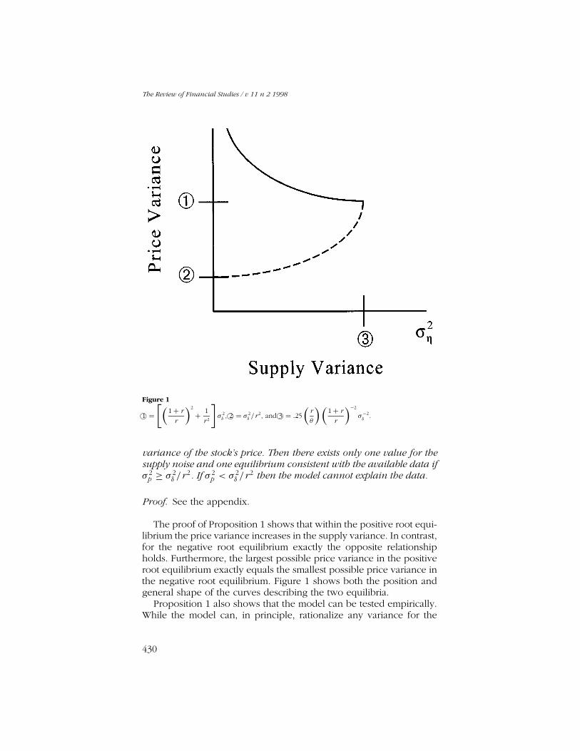
Figure 1

1© =[(

1+ r

r

)2

+ 1

r 2

]σ 2δ , 2© = σ 2

δ /r 2, and 3© = .25

(r

θ

)(1+ r

r

)−2

σ−2δ

.

variance of the stock’s price. Then there exists only one value for thesupply noise and one equilibrium consistent with the available data ifσ 2

p ≥ σ 2δ /r 2. If σ 2

p < σ 2δ /r 2 then the model cannot explain the data.

Proof. See the appendix.

The proof of Proposition 1 shows that within the positive root equi-librium the price variance increases in the supply variance. In contrast,for the negative root equilibrium exactly the opposite relationshipholds. Furthermore, the largest possible price variance in the positiveroot equilibrium exactly equals the smallest possible price variance inthe negative root equilibrium. Figure 1 shows both the position andgeneral shape of the curves describing the two equilibria.

Proposition 1 also shows that the model can be tested empirically.While the model can, in principle, rationalize any variance for the

430

Stock Price Volatility in a Multiple Security Overlapping Generations Model

price series that exceeds the variance of the dividend series dividedby r 2, it can only do so via a particular supply noise. Thus one canthink of this model as testable in the same sense one tests modelslike the consumption CAPM. If estimates of the model’s unobservableparameters seem unreasonable, then people conclude that the modeldoes not generate the observed data. Section 2 provides some insightinto this issue by showing that the model can produce reasonable es-timates for the supply variance based upon the parameters producedin past empirical studies.

1.5 Variance in a multiple security economyWhile single-security models provide numerous insights, there existmany issues that can only be addressed in a multiple security envi-ronment. This section examines the way stocks interact within the setof potential equilibria.

While a single-security economy contains two potential equilibria,the multiple security economy contains 2K potential equilibria. Nat-urally they derive from the same source: the square root term in thesolution to A. If a linear equilibrium exists the term under the squareroot in Equation (12) is a symmetric positive definite matrix. Write

0′30 = 1

4

( r

θ

)26−2η −

(1+ r

r

)2

6−1/2η 6δ6

−1/2η , (17)

where 0 represents an orthonormal matrix of eigenvectors and 3 adiagonal matrix of eigenvalues. Because Equation (17) appears withina square root in the solution for A, one can restate the far right termin A [from Equation (12)] as 0′31/20. This implies that their exist twopotential values for each diagonal element of 31/2 that are compatiblewith the equilibrium requirements. With K securities there exist Kdiagonal elements, and so there must be 2K possible solutions, eachcorresponding to a unique equilibrium. One thus has the followingproposition.

Proposition 2. With K securities in random supply there exist 2K

equilibria. These equilibria correspond to the set of feasible eigenvaluesfor the matrix in Equation (17).

In the single-security case the equilibrium in the economy dependsupon the selected root for Equation (14). When the market containsnumerous securities the square root of the eigenvalues within 3 playan analogous role. As one might suspect, the volatility conclusionsfrom the single-security case also generalize.

431

The Review of Financial Studies / v 11 n 2 1998

Proposition 3. Consider an equilibrium, and the variance of anyportfolio under that equilibrium. Then switching any eigenvalue inthe matrix 31/2 from negative to positive reduces the portfolio’s vari-ance.

Proof. See the appendix.

Clearly society would like to operate in an economy where allthe selected roots from 31/2 are positive. If some of the roots arenegative, then their exists an incentive for some organization to try andchange the equilibrium. However, this may be rather difficult since theequilibria do not, in general, associate each eigenvalue with a singlesecurity. Rather an eigenvalue determines the volatility of a mutualfund with portfolio weights determined by the associated eigenvector.To change the equilibrium an organization must somehow alter thebehavior of an entire mutual fund and not just a single security. Unlessone can credibly accomplish this task, investors will not believe thatthey are in a new equilibrium and so the old equilibrium will prevail.It seems that once a high-volatility equilibrium gets started it may bevery difficult to alter it.

While stock price volatility depends upon the selected equilibrium,production by the corporate sector does not. In fact, the model’s as-sumptions force all of the price volatility to derive from beliefs andnot an interaction of beliefs and production. However, while corpo-rate production does not depend upon the selected equilibrium, theeconomy-wide store of the risk-free asset does. In period t the to-tal value of the available risky asset equals Pt Nt , an amount that theyoung generation must turn over to the old generation via a transfer ofthe risk-free asset. If Pt differs across equilibria then so will the amountof the risk-free asset given to the older generation to consume. As aresult, while stock price volatility does not manifest itself in corporateproduction, it still influences aggregate consumption via fluctuationsin the population’s holdings of the risk-free security. This imposes an-other potential impediment to switching among equilibria. While exante everybody may prefer the low-volatility equilibrium, ex post dif-ferent generations will have opposing interests depending upon howswitching the equilibrium will influence the set of current prices.

Returning again to Equation (17), it also shows how two securitieswith identical dividend streams can trade at different prices and ex-hibit different price volatilities. A simple examination makes it clearthat6δ, the dividend variance-covariance matrix, can be singular. Onlythe supply shock matrix 6η needs to be of full rank. Thus, dependingupon the supply shocks, one can create an equilibrium in which twostocks with perfectly correlated dividend streams have different mo-

432

Stock Price Volatility in a Multiple Security Overlapping Generations Model

ments associated with their prices.7 Initially, it might seem that if thetwo stocks have different supply levels then in some sense they arenot identical. However, this is only true to a limited degree. In princi-ple, since both stocks have identical dividend streams, one can dividethe supply shocks up in any manner one wishes, without changingthe fundamentals of the economy. Thus in this case the correlationbetween the supply shocks is in some sense arbitrary. Nevertheless,if the dividend streams are identical and the prices are not, does thisopen up an arbitrage opportunity? No, providing investors have finitelives. An infinitely lived individual can buy the cheap stock, sell theexpensive stock and make a risk-free profit. However, in any finitelength of time an investor that tries this risks having the prices movefurther in the wrong direction. Thus stocks that have identical div-idend streams but different pricing patterns provide people with aprofit opportunity, but one that contains risk. The equilibrium equa-tions tell us the degree to which prices can diverge and still producedemands that balance out the supplies.

There already exist several models that can potentially reconcilethe empirical volatility results through the introduction of “noise” fromvarious sources. One contribution of this article is to show, in Theorem1, that a model with fully rational agents can produce the requisitevariances with small supply noise levels. That theorem used Equation(15) to derive its results and was based on the assumption that themarket contains only one risky security. As the next set of resultsshow, in a multiple security environment, Equation (15) can vastlyoverstate the required aggregate supply noise. Propositions 4 and 5show that under fairly mild assumptions, as the number of securitiesgrows to infinity the supply variance of the market portfolio neededto reconcile any particular aggregate price and dividend variance goesto zero. Lemma 2 then shows, under the assumption that all securitieshave independent identically distributed payoffs and supplies, thatif there exist K securities then the value of σ 2

η derived via Equation(15) will overstate the required aggregate supply variance by a factorof K 2.

There are two routes that lead to the conclusion that as the num-ber of securities goes to infinity the supply noise needed to produceany particular variance in the price innovations goes to zero. One caneither place some restrictions on the form of the variance-covariancematrix describing the supply noise or the dividend shocks. Propo-sition 4 takes the former tack and Proposition 5 the latter. For the

7 At least two other articles in this genre have produced the same result. In both DeLong et al. (1990)and Bhushan, Brown, and Mello (1997) there are two risk-free assets with identical payoffs. Withinboth models one risk-free asset has a constant price and the other a volatile price.

433

The Review of Financial Studies / v 11 n 2 1998

limiting results that follow let K both index a particular economy andrepresent the number of risky securities. Further, let nj represent thej th element of N at time t and assume that at a particular time t

Assumption 1.∑K

j=1 nj = 1 for all K , and nj ≥ 0 for all j .

Assumption 2. That the

limK→∞max{n1, . . . ,nK } → 0. (18)

Assumption 3. N ′6δN = kδ, where kδ is a constant independent of K .

Assumption 4. N ′6pN = kp, where kp is a constant independentof K .

Assumption 5. kp ≥ 1r 2 kδ.8

Assumption 1 acts to normalize the number of shares and theirsign.9 Assumption 2 states that as the number of securities goes toinfinity any one firm becomes only a small part of the economy. As-sumptions 3 and 4 hold the aggregate dividend and price varianceconstant. Finally, Assumption 5 states that stock prices exhibit “ex-cess” volatility.

An econometrician cannot observe the supply noise directly. Thusa reasonable starting point for empirical research may be to assumethat the variance-covariance matrix of the security supply is a diagonalmatrix proportional to I . If this assumption describes the economythen the next proposition shows that under Assumptions 1 through 5the aggregate supply noise goes to zero as K goes to infinity.

Proposition 4. Assume that one can write 6η as σ 2η I , where σ 2

η is ascalar. Then under assumptions 1 through 5 N

′6ηN = σ 2η goes to zero

as K goes to infinity.

Proof. From Equation (12) an equilibrium exists if and only if

1

4

( r

θ

)2I −

(1+ r

r

)2

61/2η 6δ6

1/2η (19)

is a positive semidefinite matrix. Under the assumption that 6η = σ 2η I ,

8 In Assumptions 1 through 5 the date index t has been suppressed for notational simplicity.9 If the supply of a particular stock is currently negative, one can simply change the sign on the

dividend and the stock simultaneously, and thereby leave the economy unchanged.

434

Stock Price Volatility in a Multiple Security Overlapping Generations Model

Equation (19) simplifies to

1

4

( r

θ

)2I −

(1+ r

r

)2

σ 2η6δ. (20)

If Equation (20) is a positive semidefinite matrix then pre- and post-multiplying by N must produce a nonnegative number. Using As-sumptions 1 and 2 one can prove that N ′N goes to zero as K goes toinfinity. Since 6δ is a positive definite matrix, and by Assumption 3N′6δN does not depend on K , one must have that σ 2

η goes to zero.Since N

′6ηN = σ 2η , this proves that the aggregate supply variance goes

to zero if an equilibrium exists. Finally, given the restrictions imposedby Assumption 5, one can always select a value for σ 2

η that satisfiesAssumption 4 and causes an equilibrium to exist by solving Equation(13) and picking positive or negative eigenvalues as needed. Sincethe proof follows along the same lines as the proof for Proposition 1it is not repeated here.

While Proposition 4 allows for a general dividend covariance matrixit imposes assumptions on the supply’s covariance structure. Since thesupply cannot be observed directly it may be possible to construct amore robust statistical test by restricting 6δ instead as in the nextproposition.

Proposition 5. Assume that as K goes to infinity the smallest eigen-value of the matrix6δ approaches a number strictly greater than zero.Then under Assumptions 1 through 5 the supply variance of the marketportfolio N ′6ηN goes to zero.

Proof. An equilibrium exists if and only if the matrix of Equation (19)is positive semidefinite, and thus

limK→∞N ′61/2

η 6δ61/2η N → 0 (21)

since Assumptions 1 and 2 imply N ′N goes to zero as K goes toinfinity. Let Y = 61/2

η N . Then using Equation (21) one has

N ′61/2η 6δ6

1/2η N = Y ′6δY ≥ νminY ′Y (22)

where νmin represents the smallest eigenvalue of 6δ. By assumptionνmin approaches a strictly positive number as K goes to infinity. ThusEquation (21) can only hold if Y ′Y goes to zero, which proves theproposition since Y ′Y = N ′6ηN .

Propositions 4 and 5 show that within a multiple security environ-ment very small shocks can produce large price changes. To obtain

435

The Review of Financial Studies / v 11 n 2 1998

some intuition as to just how quickly the supply shock declines, con-sider what happens as one divides the economy’s risky capital assetinto K identically sized independent pieces. As the following lemmashows this divides the required supply variance by K 2.

Lemma 2. Assume 6η = σ 2η I , 6δ = σ 2

δ I , and ni = 1/K in addition toAssumptions 1 through 5. As K increases assume that the equilibriumonly uses either the positive or negative roots from the matrix 31/2.Then σ 2

δ = K kδ and if σ 2η = σ̂ 2

η equals the solution in the 1 securitycase then σ 2

η = σ̂ 2η /K in the K security case. The latter result implies

that the supply variance of the market portfolio equals σ̂ 2η /K

2.

Proof. Since 6δ = σ 2δ I and ni = 1/K the dividend variance will equal

kδ if σ 2δ = K kδ. Use this to substitute out σ 2

δ in Equation (13). Nextreplace σ 2

η with σ̂ 2η /K to verify that this keeps N ′6pN constant. Finally,

with ni = 1/K , and σ 2η = σ̂ 2

η /K it follows that the supply variance ofthe market portfolio equals σ̂ 2

η /K2.

Lemma 2 shows that in practice a very small aggregate supply vari-ance can easily produce a very large price variance. Empirically thelemma indicates that estimates of the model based only on the aggre-gate market index will probably overestimate the supply variance bya factor of perhaps several hundred.

2. Empirical Implications

2.1 Calibrating the modelIntuitively one would like the model to explain the data with “rela-tively small” supply shocks. However, providing a useful definitionfor “relatively small” turns out to be fairly complex. Since the presentanalysis seeks to explain market volatility it seems intuitive to comparethe supply volatility to the wealth volatility induced from one share ofstock. For notational consistency define πt as the wealth from holdingone share of stock this period (i.e., πt = Pt ) and πt+1 as the wealthfrom selling the share next period and cashing in its dividend (i.e.,πt+1 = Pt+1 + Dt+1). Further define σ 2

π as the per period variance inπ , so that σ 2

π = E (πt+1 − πt )2 given πt . At this point one may be

tempted to compare ση directly with σπ . Unfortunately a direct com-parison is not productive since ση and σπ are in inverse units to eachother. To see this consider a unit of account such that there existsonly one share of stock and fix both ση and σπ . Now consider thesame economy but split the stock into two shares. This doubles thenumber of shares which doubles ση and simultaneously cuts the div-

436

Stock Price Volatility in a Multiple Security Overlapping Generations Model

idend per share in half, thereby dividing σπ in half. Thus dependingon the normalization selected one can set ση/σπ to any value. For-tunately one can easily circumvent this problem by normalizing withthe appropriate units, thereby producing a scale-free test statistic

S = ση

N

π

σπ= ση

N

P

σπ. (23)

If S equals one the supply shocks and wealth shocks have similarmagnitudes. Larger values indicate that ση predominates, and smallervalues that σπ predominates. Since it seems unlikely that the aggregatesupply shocks exceed the stock price shocks, a “good” model shouldproduce fairly small values for S .

While Equation (23) takes care of the scaling problem it requiresone to know both N and P , which for fairly obvious reasons do notappear among the statistics generally reported. However, this prob-lem can be circumvented by requiring N and P to take on valuesthat will induce the model to produce statistics that correspond withwell-accepted properties associated with market returns. Under a stan-dard CAPM-like model, with dividends that follow a random walk,Pt = Dt/r ∗ where r ∗ > r represents the dividend discount rate. Onecan then write the return variance σ 2

r as

σ 2r =

(1+ r ∗)2σ 2δ

D2t

. (24)

Well-known estimates from Ibbotson Associates (1989) place σ 2r at

.209 for annual data.10 Thus filling in Equation (24) with σ 2r at .209

and a particular study’s reported value for σ 2δ and r ∗ one obtains the

implicit price scale that will induce the model to produce a sensiblereturn series. The value of N in Equation (23) is somewhat simplerto find. Let W represent the dollar value of the wealth held by eachtrader in the stock market. Then by definition Wt = Pt N . Substitutingthis into Equation (23) eliminates N from the equation.

To obtain S in terms of observable variables one now only needsan estimate of σπ . Since πt+1 = Pt+1+Dt+1 and πt = Pt it follows that

σπ =(

1+ r ∗

r ∗

)σδ (25)

since Pt = Dt/r ∗.

10 However, as the text will shortly explain, the S value does not depend upon σ 2r .

437

The Review of Financial Studies / v 11 n 2 1998

Using Equations (24) and (25) along with the substitutions N =Wt/Pt and Pt = Dt/r ∗ the statistic S reduces to

S = σησδ(1+ r ∗)Wt r ∗σ 2

r

. (26)

Even with the values of σδ and σP reported by a study the modelcannot pin down ση without knowledge of θ . Under a mean-varianceanalysis a standard CAPM-type model will produce the first-order con-dition

r ∗ − r − θσ 2δ (1+ r ∗)2

Xt

rsDt= 0. (27)

Solving this for θ one obtains

θ = r ∗(r ∗ − r )Dt

σ 2δ (1+ r ∗)2Xt

. (28)

Now use Equation (24) to eliminate σδ from the above equation, alongwith Pt = Dt/r ∗ and Wt = Pt Xt , to produce

θ = r ∗ − r

σ 2r Wt

. (29)

Using the above value for θ , along with values from a study for σδ andσP , Equation (15) will yield the value of ση needed to reconcile themodel with the reported empirical results. Notice that the implied riskaversion parameter is not scale-free. Moving from dollars to cents willmultiply Wt by 100 while leaving all the other variables on the right-hand side of Equation (29) unchanged. Thus the value of θ dependsinversely on the units of account selected. Normally people think ofpreference parameters as exogenous to the model and independentof the currency unit. But the parameter θ represents risk aversion perunit of consumption as measured in the unit of account. Changingthe unit of account changes the risk aversion through the change intranslation from currency to consumption units.

It may appear that the estimate of S will depend heavily upon thevalues used for σ 2

r and Wt . In fact, S is invariant to changes in either ofthese parameters. To see why, notice that θ depends inversely uponboth σ 2

r and Wt and so does S . At the same time one can see fromEquation (15) that ση depends inversely upon θ . Thus the changesinduced to the model through both σ 2

r and Wt leave S unchanged.Intuitively the reason this occurs is that S has been made into a scale-free statistic, and the values of σ 2

r and Wt depend arbitrarily upon theselected scale.

438

Stock Price Volatility in a Multiple Security Overlapping Generations Model

Table 1Model statistics implied by Shiller’s (1981b) equa-tion (I-3) empirical estimates

r .04 .05 .06 .071− σδ/rσp 0.505 0.622 0.699 0.754

SK = 1 0.552 0.502 0.458 0.422K = 30 0.018 0.017 0.015 0.026

In all cases the estimates imply that the negative rootequilibrium holds.Row labeled r : interest rate used in each column. Row labeled1 − σδ/rσp: fraction of the price variance that cannot beaccounted for in the standard fixed supply dividend discountmodel. West [1988, Equation (17)] uses an identical measuremultiplied by 100. Rows labeled S : numerical value of Sunder the given interest rate, the return standard deviation,and the number of traded securities under the assumptions ofLemma 2.

Among the many variance inequality tests of the efficient marketshypothesis that have been explored one of the earliest is

σ(1P) ≤ σ(1D)/√

2r 3/(1+ 2r ) (30)

which can be found in Shiller (1981b) with 1D defined as Dt −Dt−1.Using 10-year intervals Shiller (1981b) finds that σ(1P) = 69.4, andσ(1D) = 16.5. Thus, in his test, markets can only be efficient if theannual interest rate remains below 3.2%. Since actual discount ratesappear to lie above 4%, the model’s predictions do not conform withthe data.

Since the model presented in Section 1 predicts that stock pricevolatility has both a dividend and supply component, it can potentiallyreconcile Shiller’s (1981b) estimates with an environment populatedby rational traders. By adjusting ση Equation (15) can produce anexpected price volatility equal to that reported in past empirical workgiven any previously estimated dividend variance. However, in orderto calculate ση from Equation (15) and S from Equation (26) estimatesof the dividend discount factor and the return variance are needed.Based upon the values used in West (1989), Mankiw, Romer, andShapiro (1991), and Campbell and Kyle (1993) an appropriate discountfactor seems to lie between 4% and 7%.

Table 1 provides values of the model’s parameters that will pro-duce data consistent with Shiller’s (1981b) estimates in a one-securityenvironment. However, as Lemma 2 shows, the resulting estimatesof the aggregate supply standard deviation will exceed the supplystandard deviation in a multiple security economy by a factor of K .Thus the single risky security aggregate supply standard deviationfigures calculated in the table should be viewed as extremely con-

439

The Review of Financial Studies / v 11 n 2 1998

servative upper bounds. To provide a more realistic scenario figuresare also provided under a 30-security economy based on the assump-tions leading to Lemma 2. Employing the empirical estimates withinthe model requires that the economy operate under the negative rootequilibrium. Thus it appears that the additional equilibrium found inthis model provides a useful degree of freedom with which to explainthe data.

Notice that the column labeled 1 − σδ/rσp shows that dividendshocks explain less than half of the price volatility. Nevertheless, thecalculated value of S lies well below 1. The model, therefore, explainsover half the price volatility with relatively small supply shocks. Re-call that supply shocks are generally taken to represent changes inhuman capital and other illiquid assets. As such it seems likely thatthe variance of these supply shocks should be small relative to thestock return shocks. Table 1 indicates that the model can produceestimates which conform to this intuition.

Naturally, over time Shiller’s (1981b) statistical model has been su-perceded by more powerful second-generation tests. These tests haveconfirmed Shiller’s conclusions and generally produce even strongerrejections of the standard dividend discount model. Since the modelcan reconcile Shiller’s results with values of S under .03 (with 30 secu-rities) it produces even smaller S values when applied to the second-generation tests. Overall then, the model shows that a combinationof relatively small random supply shocks and finitely lived agents canproduce stock market data similar to what we observe.

3. A Trend Stationary Model

3.1 Modified model and its solutionThe empirical literature has generally sought to reconcile the stockmarket dividend and price data by assuming that dividends followa random walk. Thus the same assumptions were employed in Sec-tion 1. However, there are two reasons for considering a model witha mean reverting dividend process. First, a number of statistical stud-ies, such as DeJong and Whiteman (1991), have come to the conclu-sion that dividends are mean reverting. Thus one would hope thatadding this feature to a model will not invalidate its conclusions. Sec-ond, a mean reverting process makes it more difficult to reconcilethe dividend-price data under the standard dividend discount model.This naturally raises the question as to how well the current modelperforms under a mean reverting dividend process. As the analysisin this section shows, under the volatile equilibrium, making eitheror both the dividends or the supply of the risky asset mean revertingincreases the sensitivity of stock prices to supply shocks.

440

Stock Price Volatility in a Multiple Security Overlapping Generations Model

To relax the random walk assumptions used so far, assume thatdividends are generated via the following formula

Dt = Dt−1 − β(Dt−1 − D̄)+ δt , (31)

and the stock supply by

Nt = Nt−1 − α(Nt−1 − N̄ )+ ηt . (32)

Here D̄ represents a vector of constants toward which dividends moveover time, while N̄ represents a similar vector for the stock supply.The terms β and α are scalar constants that determine the speed atwhich the processes revert toward their stationary values. Setting βor α to zero causes Equations (31) and (32) to revert back to theirrespective form in Section 1.

Since the analysis remains basically identical to that found in Sec-tion 1, only the results are presented here. The equation relating pricesto the underlying state variables now includes a constant component(K × 1) vector C , and thus prices equal

Pt = ANt + BDt + C . (33)

Repeating the steps found earlier one finds that A, B, and C satisfythe following equations:

A = −1

2

(α + r

θ

)6−1η

+(

1

4

(α + r

θ

)2

6−2η −

(1+ r

β + r

)2

6−1/2η 6δ6

−1/2η

)1/2

, (34)

B = 1− ββ + r

I , (35)

and

C = (1+ r )β

(β + r )rD̄

+ αr

− 1

2

(α + r

θ

)6−1/2η

+(

1

4

(α + r

θ

)2

6−2η −

(1+ r

β + r

)2

6−1/2η 6δ6

−1/2η

)1/2N̄ . (36)

While C seems to add a great deal of complexity to the solution, itdrops out of the variance-covariance calculations. Thus, as the next

441

The Review of Financial Studies / v 11 n 2 1998

subsection will show, a trend stationary dividend does not manifestlychange the model’s qualitative properties.

3.2 Implied price varianceThe variance-covariance matrix of prices can be calculated as

E (Pt+1 − Pt )(Pt+1 − Pt )′ = Ab6η + α2(Nt − N̄ )(Nt − N̄ )′cA′

+ Bb6δ + β2(Dt − D̄)(Dt − D̄)′cB ′. (37)

To obtain the formula only in terms of endogenous variables one canuse Equations (34) and (35) to eliminate A and B from Equation (37).Notice that increasing α and β from 0 does not materially alter theequilibrium’s properties. This becomes even more apparent in thescalar case. When there exists only one risky stock, A reduces to

A = −1

2

(α + r

θ

)σ−2η ± σ−2

η

√1

4

(α + r

θ

)2

−(

1+ r

β + r

)2

σ 2δ σ

2η . (38)

Because the basic structure of Equation (38) is identical to Equation(14) the conclusions reached in earlier sections remain unchanged.However, allowing for mean reversion allows one to prove the fol-lowing additional results.

Proposition 6. Within the volatile equilibrium, increasing the speedof mean reversion in either the dividend or supply process increasesthe sensitivity of the stock price to supply shocks. Formally, ∂A/∂α < 0and ∂A/∂β < 0 under the negative root equilibrium.

4. Conclusion

The relative volatility of stock prices to the dividend process has pro-duced a long string of papers. No doubt this will continue into thedistant future. This article shows that one can produce large price-dividend standard deviation ratios in a model with fully rational agents.More importantly one can produce these statistics with a rather mod-est variance in the unobservable supply of stock. The model can fitreported relative price-dividend standard deviation ratios with supplyshocks that are generally less than 10% as large as the price changesbeing explained. This seems like a useful trait for any model to pos-sess if one suspects that the capital asset supply variance is muchsmaller than the aggregate stock price variance.

Another feature brought out by the analysis is the potential im-portance a multiple security environment can play in the market’s

442

Stock Price Volatility in a Multiple Security Overlapping Generations Model

aggregate volatility. Simply put, the greater the number of securitiesthe smaller the required supply variance to generate any particularvariance for the aggregate price index.

Appendix: Proofs for Claims in the Main Body of the Text

Lemma 1. The matrix A mapping the supply of shares to prices is sym-metric and has the following solution:

A = −1

2

r

θ6−1η +

[1

4

( r

θ

)26−2η −

(1+ r

r

)2

6−1/2η 6δ6

−1/2η

]1/2

. (A1)

Proof. To prove A is symmetric, note that from Equation (11) A solves

A6ηA′ + r

θA +

(1+ r

r

)2

6δ = 0. (A2)

The first and third terms are symmetric since 6η and 6δ are symmet-ric variance-covariance matrices. Since r and θ are scalars, A must besymmetric. This allows one to replace the A′ term with A in Equa-tion (A2). Now pre- and postmultiply by 61/2

η and let Y = 61/2η A61/2

η ,thereby producing

Y 2 + r

θY +

(1+ r

r

)2

61/2η 6δ6

1/2η = 0, (A3)

which is a quadratic matrix equation. To solve for Y , complete thesquare by adding and subtracting 1

4 (rθ)2I . After some minor algebra

this generates(Y + .5 r

θI)2= .25

( r

θ

)2I −

(1+ r

r

)2

61/2η 6δ6

1/2η , (A4)

and allows one to conclude

Y = −1

2

r

θI +

(1

4

( r

θ

)2I −

(1+ r

r

)2

61/2η 6δ6

1/2η

)1/2

. (A5)

Finally, substitute out for Y by using the relationship Y = 61/2η A61/2

η ,and then pre- and postmultiply by 6−1/2

η to finish the proof.

Proposition 1. Assume that an econometrician knows the risk aver-sion of the population, the variance of the dividend series, and thevariance of the stock’s price. Then there exists only one value for the

443

The Review of Financial Studies / v 11 n 2 1998

supply noise and one equilibrium consistent with the available data ifσ 2

p ≥ σ 2δ /r 2. If σ 2

p < σ 2δ /r 2 then the model cannot explain the data.

Proof. The proposition can be proved in three steps. The first stepshows that in the positive root equilibrium σ 2

p increases in σ 2η . The

second step shows that in the negative root equilibrium σ 2p decreases

in σ 2η . Finally, the third step shows that the largest value σ 2

p takes onin the positive root equilibrium equals the smallest value it takes onin the negative root equilibrium.

Step 1, begin with the positive root equilibrium. In this case theprice variance can be written as

σ 2p =

1

2

( r

θ

)2−(

1+ r

r

)2

σ 2η σ

2δ −

r

θ

√1

4

( r

θ

)2−(

1+ r

r

)2

σ 2η σ

2δ

σ−2η

+ 1

r 2σ 2δ , (A6)

which is identical to the negative root of Equation (16) except for thesign in front of the square root symbol. One can simplify the algebraby using the precision of η rather than its variance. Thus let ρη = σ−2

η

and substitute into Equation (A6), and then differentiate Equation (A6)with respect to ρη producing

∂σ 2p

∂ρη= 1

2

( r

θ

)2−

12

rθ

[12

(rθ

)2ρη −

(1+r

r

)2σ 2δ

]√

14

(rθ

)2ρ2η −

(1+r

r

)2σ 2δ ρη

. (A7)

While Equation (A7) cannot immediately be signed for all ρη it can besigned at the lower bound of ρη. To generate a real solution to Equa-tion (14) the term inside the radical sign must be positive. Therefore

ρη ∈[4( r

θ

)−2(

1+ r

r

)2

σ 2δ ,∞

]. (A8)

Now divide the top and bottom of the last term in Equation (A7) byρη and then evaluate as ρη goes to infinity. After some algebra, thisproduces

limρη→∞

∂σ 2p

∂ρη∝ − r

θ< 0. (A9)

Thus at ρη’s upper bound ∂σ 2p /∂ρη is negative. To prove this holds for

444

Stock Price Volatility in a Multiple Security Overlapping Generations Model

all ρη, consider the second derivative

∂2σ 2p

∂ρ2η

∝(

1+ r

r

)4

σ 4δ > 0, (A10)

which arises after some extensive but straightforward algebra. Since∂σ 2

p /∂ρη < 0 at the upper bound for ρη and since ∂2σ 2p /∂ρ

2n > 0 for

all ρη, it follows that ∂σ 2p /∂ρη < 0 for all ρη. Translating back from ρη

to σ 2η , one has now shown that ∂σ 2

p /∂σ2η > 0 for all σ 2

η .Step 2 is to consider the negative root equilibrium. Again use ρη

and differentiate Equation (14), yielding

∂σ 2p

∂ρη= 1

2

( r

θ

)2+

rθ

[12

(rθ

)2 − ( 1+rr

)2σ 2δ

]√

14

(rθ

)2ρ2η −

(1+r

r

)2σ 2δ ρη

. (A11)

Since the term inside the square root must be positive, and the brack-eted term in the numerator is bigger then the term inside the squareroot, one immediately has that ∂σ 2

p /∂ρη > 0. This in turn implies that∂σ 2

p /∂σ2η < 0 for all permissible σ 2

η .Step 3 is to consider the value σ 2

p in the positive root equilibrium.Since its value increases in σ 2

η the maximal value of σ 2p must oc-

cur at the maximal value for σ 2η . Plugging this in and using σ̄ 2

η =14 (

rθ)2( 1+r

r )−2σ−2δ produces

σ 2p

∣∣∣σ 2η=σ̄ 2

η

=(

1+ r

r

)2

σ 2δ +

σ 2δ

r 2. (A12)

Under the negative root equilibrium, the smallest value of σ 2p must

occur at the maximal value σ 2η since in the negative root equilibrium σ 2

p

declines in σ 2η . Plugging this into Equation (14) produces an equation

identical to Equation (A12). Thus each equilibrium covers a disjointset of values for σ 2

p .

Proposition 3. Consider an equilibrium and the variance of anyportfolio under that equilibrium. Then switching any eigenvalue inthe matrix 31/2 from negative to positive reduces the portfolio’s vari-ance.

Proof. Let X represent an arbitrary portfolio. Then the variance of thatportfolio can be written as

σ 2X = X ′

[A6ηA

′ + 1

r 26δ

]X . (A13)

445

The Review of Financial Studies / v 11 n 2 1998

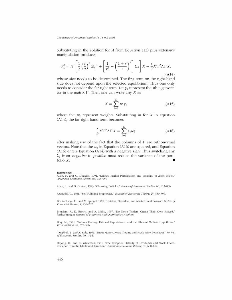
Substituting in the solution for A from Equation (12) plus extensivemanipulation produces

σ 2X = X ′

[1

2

( r

θ

)26−1η +

[1

r 2−(

1+ r

r

)2]6δ

]X − r

θX ′0′30X ,

(A14)whose size needs to be determined. The first term on the right-handside does not depend upon the selected equilibrium. Thus one onlyneeds to consider the far right term. Let γi represent the ith eigenvec-tor in the matrix 0. Then one can write any X as

X =K∑

i=1

wiγi (A15)

where the wi represent weights. Substituting in for X in Equation(A14), the far right-hand term becomes

r

θX ′0′30X =

K∑i=1

λiw2i (A16)

after making use of the fact that the columns of 0 are orthonormalvectors. Note that the wi in Equation (A16) are squared, and Equation(A16) enters Equation (A14) with a negative sign. Thus switching anyλi from negative to positive must reduce the variance of the port-folio X .

ReferencesAllen, F., and G. Douglas, 1994, “Limited Market Participation and Volatility of Asset Prices,”American Economic Review, 84, 933–955.

Allen, F., and G. Gorton, 1993, “Churning Bubbles,” Review of Economic Studies, 60, 813–836.

Azariadis, C., 1981, “Self-Fulfilling Prophecies,” Journal of Economic Theory, 25, 380–396.

Bhattacharya, U., and M. Spiegel, 1991, “Insiders, Outsiders, and Market Breakdowns,” Review ofFinancial Studies, 4, 255–282.

Bhushan, R., D. Brown, and A. Mello, 1997, “Do Noise Traders ‘Create Their Own Space’?,”forthcoming in Journal of Financial and Quantitative Analysis.

Bray, M., 1981, “Futures Trading, Rational Expectations, and the Efficient Markets Hypothesis,”Econometrica, 49, 575–596.

Campbell, J., and A. Kyle, 1993, “Smart Money, Noise Trading and Stock Price Behaviour,” Reviewof Economic Studies, 60, 1–34.

DeJong, D., and C. Whiteman, 1991, “The Temporal Stability of Dividends and Stock Prices:Evidence from the Likelihood Function,” American Economic Review, 81, 600–617.

446

Stock Price Volatility in a Multiple Security Overlapping Generations Model

De Long, J., A. Shleifer, L. Summers, and R. Waldmann, 1990, “Noise Trader Risk in FinancialMarkets,” Journal of Political Economy, 98, 703–738.

Diamond, D., and R. Verrecchia, 1981, “Informational Aggregation in a Noisy Rational ExpectationsEconomy,” Journal of Financial Economics, 9, 221–235.

Eden, B., and B. Jovanovic, 1994, “Asymmetric Information and the Excess Volatility of StockPrices,” Economic Inquiry, 32, 228–235.

Glosten, L., 1989, “Insider Trading, Liquidity, and the Role of the Monopolist Specialist,” Journalof Business, 62, 211–235.

Ibbotson Associates, Inc., 1989, Stocks, Bonds, Bills, and Inflation 1989 Yearbook, IbbotsonAssociates, Chicago.

Jackson, M., 1994, “A Proof of the Existence of Speculative Equilibria,” Journal of Economic Theory,64, 221–233.

Kleidon, A., 1986, “Variance Bounds Tests and Stock Price Valuation Models,” Journal of PoliticalEconomy, 94, 953–1001.

Kraus, A., and M. Smith, 1997, “Endogenous Sunspots, Pseudo-bubbles, and Beliefs About Beliefs,”forthcoming Journal of Financial Markets.

Mankiw, N. G., D. Romer, and M. Shapiro, 1985, “An Unbiased Reexamination of Stock MarketVolatility,” Journal of Finance, 40, 677–687.

Mankiw, N. G., D. Romer, and M. Shapiro, 1991, “Stock Market Forecastability and Volatility: AStatistical Appraisal,” Review of Economic Studies, 58, 455–477.

Marsh, T., and R. Merton, 1986, “Dividend Variability and Variance Bounds Tests for the Rationalityof Stock Market Prices,” American Economic Review, 76, 483–498.

Paul, J., 1994, “Information Aggregation Without Exogenous ‘Liquidity’ Trading,” working paper,University of Michigan.

Romer, D., 1993, “Rational Asset-Price Movements Without News,” American Economic Review,83, 1112–1130.

Shiller, R., 1981a, “Do Stock Prices Move Too Much to be Justified by Subsequent Changes inDividends?,” American Economic Review, 71, 421–435.

Shiller, R., 1981b, “The Use of Volatility Measures in Assessing Market Efficiency,” Journal ofFinance, 36, 291–304.

Subrahmanyam, A., 1991, “A Theory of Trading in Stock Index Futures,” Review of FinancialStudies, 4, 17–51.

Tirole, J., 1985, “Asset Bubbles and Overlapping Generations,” Econometrica, 53, 1071–1100.

Wang, J., 1993, “A Model of Intertemporal Asset Prices Under Asymmetric Information,” Reviewof Economic Studies, 60, 249–282.

Wang, J., 1994, “A Model of Competitive Stock Trading Volume,” Journal of Political Economy,11, 127–168.

West, K., 1988, “Dividend Innovations and Stock Price Volatility,” Econometrica, 56, 37–61.

447