QEDQueen’s Economics Department Working Paper No. 1325

Stock-based Compensation Plans and Employee Incentives

Jan ZabojnikQueen’s University

Department of EconomicsQueen’s University

94 University AvenueKingston, Ontario, Canada

K7L 3N6

6-2014

Stock-based Compensation Plans and Employee

Incentives∗

Ján Zábojníka

June 17, 2014

Abstract

Standard principal-agent theory predicts that large firms should not use employee

stock options and other stock-based compensation to provide incentives to non-executive

employees. Yet, business practitioners appear to believe that stock-based compensation

improves incentives, and mounting empirical evidence points to the same conclusion.

This paper provides an explanation for why stock-based incentives can be effective.

In the model of this paper, employee stock options complement individual measures

of performance in inducing employees to invest in firm-specific knowledge. In some

situations, a contract that only consists of options is more effi cient than a contract

based solely on individual performance.

Keywords: Stock-based Compensation, Employee Stock Options, Optimal Incentive

Contracts, Firm-specific Knowledge

JEL codes: D86, J33, M52

∗ I thank seminar participants at Cornell University (Johnson), the Queen’s School of Business, and theUniversity of Rotterdam for helpful comments and suggestions. I have also benefited from discussions withPaolo Fulghieri, Ming Li, Paul Oyer, and Wolfgang Pesendorfer, from comments offered by Ilona Babenko,and from Jonathan Lee’s excellent research assistance. The financial support provided by the SSHRC isgratefully acknowledged.a Department of Economics, Queen’s University, Kingston, Ontario K7L 3N6, Canada. E-mail: zabo-

jnik@econ.queensu.ca.

1

1 Introduction

Employee stock options, restricted stock, stock purchase plans, and other equity-based pay

represent a substantial part of compensation for millions of U.S. employees. The National

Center for Employee Ownership estimates that as of 2013, there were almost 11,000 employee

stock ownership plans and 10 million employees participated in plans that provide stock

options or other equity based compensation to most or all employees.1 Such equity plans for

employees are quite common even in very large companies. Well known companies that use

broad-based stock option plans include Apple, Intel, EDS, Microsoft, Oracle, AT&T, Merck,

DuPont, PepsiCo, Procter & Gamble, Kimberly-Clark, and others.

Despite its prevalence in practice, economists find the use of equity-based compensation

for rank-and-file employees puzzling. The received wisdom is that while stock and stock

options may be good incentive tools for a firm’s top executives, they are not suitable for

motivating lower level employees. This is because stock-based compensation imposes too

much risk on workers, as it ties their rewards to the value of the whole company on which

an individual worker in a large firm has negligible influence. If local or individual measures

of performance are available, the argument goes, then it should be more effi cient to provide

incentives using these local and individual measures rather than relying on stock based

compensation such as option grants.2

This argument is perhaps most strikingly presented in Oyer and Schaefer (2005). They

calibrate a standard agency model to data on actual grants of stock options to middle-level

employees, and conclude that if the option grants in the studied firms were indeed used for

motivational purposes, the typical firm in their sample “would be paying each employee many

thousands of dollars in risk premium in order to generate added effort that the employee

values at less (often much less) than $100.”(p. 131). This appears to be a vastly ineffi cient

way to provide incentives. Oyer and Schaefer therefore argue that firms provide stock-based

compensation for reasons other than incentive provision, such as sorting and retention.3

As convincing as the above argument sounds, the incentive role of option grants seems

intuitively appealing and the notion that equity-based plans motivate employees is common

in the popular press and among business practitioners. For example, Andrew Grove, the then

chairman of Intel, argued that “When you have a company where practically all employees

. . . are stock option holders or stock owners, their motivation . . . is vectored closer to the

1http://www.esop.org/2Throughout the paper, the discussion will be couched mostly in terms of employee stock options, but the

theory applies also to restricted stock grants, stock purchase plans, and other equity-based compensation.3See also Oyer and Schaefer (2003).

2

interests of the company, and the whole organization works a lot better” (Kiechel, 2003).

A similar sentiment is expressed by John Doerr, a partner at Kleiner Perkins Caufield &

Byers (one of the largest venture capital firms in the world): “Awarding employees options

motivates them, and aligns their interests with shareholders”(Marshall, 2003). This intuition

also seems to be born out in a growing number of empirical studies on broad-based option

plans, including Core and Guay (2001), Kedia and Mozumdar (2002), Sesil at al (2002),

Ittner, Lambert, and Larcker (2003), Black and Lynch (2004), Hochberg and Lindsey (2010),

and Bryson and Freeman (2013), who all document that option grants and subsidized stock

purchase plans have incentive effects. For example, Hochberg and Lindsey (2010) find a

positive, causal relationship between the implied per-employee incentives of non-executive

options and subsequent firm operating performance.

This paper provides a theoretical foundation for the argument that broad-based stock

option plans can provide meaningful incentives. The key idea is that certain kinds of effort are

easier to motivate with stock options than with contracts based on individual performance.

In particular, the standard conclusion about poor incentive properties of broad-based option

plans is informed by models in which workers simply exert effort in the production process;

a typical example would be a maintenance worker who needs to be motivated to sweep the

floor or a sales person who needs incentives to sell the firm’s product. But in many firms,

such as high-tech firms, it is not enough that an employee simply exerts effort in the direction

pointed by her supervisor. Rather, in order to be productive and to be able to handle their

jobs, these firms’employees first need to learn intricate details about various aspects of their

company’s operations.

As a concrete example, consider the employees of Intel’s product development department

and suppose they are developing a new chip for which Apple is a potential customer. The

Intel engineers could simply develop the chip without worrying about questions such as When

will Apple transition to the next generation chips?, What are the characteristics of an ideal

chip from Apple’s perspective?, and What volume will they need? But if they actually take

the time to learn about the needs of their customers from Apple, the engineers can better

time their development efforts, better target the properties of the new chip to Apple’s needs,

and so on. All of this makes their efforts more valuable to Intel.

This paper takes it as a starting point that firms have a need to motivate this kind

of firm-specific knowledge acquisition and shows that stock-based compensation plans are

particularly suitable for this purpose. The idea is that the same knowledge that helps a

worker to better perform her job can also help her to better gauge the firm’s future prospects.

3

This private information about the firm’s prospects in turn allows the worker to better time

the exercise of her options and the sale of the shares, which provides her with powerful

incentives to acquire the firm-specific information.

The mechanism described above is broadly consistent with the evidence on informed

trading by firm insiders. In particular, there is overwhelming evidence that insider trading

indeed takes place and that it is profitable. Betzer et al (forthcoming), for example, find

that only 32.1% of the insider trades appear to be non-strategic. Bris (2005), Keown and

Pinkerton (1981), Meulbroek (1992), Seyhun (1992), and others provide additional evidence

on the prevalence of insider trading, both legal and illegal. Moreover, Roulstone (2003)

documents that firms that impose restrictions on trading by their insiders pay higher total

compensation (4% - 13%), which suggests not only that employees view insider trading as

profitable but also that they are willing to take pay cuts to be able to engage in it. He also

finds that the firms that limit insider trading use stronger incentives than the firms that

do not restrict insider trading, which is consistent with this paper’s premise that insider

trading provides incentives. Finally, the evidence shows that it is not just the top managers

who benefit from insider trading. Using data on employee stock purchase plans (ESPPs)

and on option exercises, a recent paper by Babenko and Sen (2014) documents that rank-

and-file employees have private information about their firm’s future performance which has

not been incorporated into the firm’s stock price. Specifically, Babenko and Sen show that

higher purchases through ESPPs (which are typically open to all employees, often with the

exception of top executives) tend to be followed by better stock price performance, whereas

option exercises tend to be negatively related to future abnormal returns.4 This corroborates

the earlier evidence in Huddart and Lang (2003), whose data show that stock option exercise

decisions of relatively junior employees contain at least as much private information as the

exercise decisions of more senior employees.

The model explored in this paper has two periods. In the first, a representative worker

invests in specific knowledge that increases her productivity with her current employer, such

as learning about the details of the production process, the customers’needs, the suppliers’

possibilities, the competencies of the worker’s superiors and co-workers, and so on. In the

second period, the worker takes an action that generates a positive expected return for the

company if and only if the worker possesses specific knowledge. The specific knowledge also

allows the worker to better assess the future prospects of the whole company, which in the

4The potential returns are quite significant. Babenko and Sen (p. 29) report that “A trading strategythat goes long in the firms that are in the top quartile of employee stock purchases and short in the firms inthe bottom quartile earns 10% in annual abnormal returns.”

4

model is captured by the assumption that the firm has assets in place that are not directly

affected by the worker’s action, but whose value is apparent to an informed worker.

The contract that the firm offers to the worker consists of a stock-based component

that depends on the value of the whole company, such as employee stock options, and of

a bonus based on the revenue she generates for the company. As in the standard theories,

the advantage of the bonus is that it ties the risk-averse worker’s pay to a measure of her

individual performance, which may be less variable and more directly affected by the worker’s

actions than the value of the whole company.

The central premise of this paper is that the advantage of stock-based compensation

is that its value to the worker depends on how well she is informed about the company’s

prospects, which gives her an incentive to invest in specific knowledge. Accordingly, the

paper’s first main result is that it is optimal to include options in the worker’s incentive

contract even if the firm has access to an individual measure of her performance that is

a suffi cient statistic for the firm’s market value with respect to the worker’s action. This

result stands in contrast to the intuition (explained earlier) that one might have based on

the textbook principal-agent model.

The paper also shows that stock option-based incentives are not useful just on the margin,

but can be quite powerful – for some parameter values, a pure stock-option contract is

much more effi cient than a contract based solely on the individual measure of the worker’s

performance. In fact, there are situations in which a pure bonus contract is so ineffi cient that

the company prefers that the worker remains uninformed, whereas a pure option contract

comes close to achieving the first best outcome, even in large firms.

Related literature

In the absence of a compelling incentive-based theory of employee stock-options, the

literature has focused on alternative explanations. Among these, the most prominent is

probably the retention argument, formalized by Oyer (2004). In Oyer’s theory, stock options

help firms to retain employees when the employees’outside opportunities vary with market

conditions. Given that renegotiating a worker’s employment contract whenever the market

conditions change may be costly and impractical, the firm tries to design the worker’s pay so

as to automatically track her outside option. Oyer shows that an option grant may provide

a relatively easy way to achieve this.

Although turnover concerns are not central to the present paper, the theory developed

here does shed some light on the retention effects of stock options —in particular, similar

to Oyer (2004), it predicts that a broad-based stock option plan will reduce subsequent

5

employee turnover. However, the mechanism that gives rise to this relationship differs from

the one proposed in Oyer (2004). Rather than tracking the workers’outside opportunities,

options in the current model discourage turnover because they motivate accumulation of

firm-specific knowledge, which in turn makes switching employers more costly. In contrast

to Oyer’s theory, the current model suggests that the negative relationship between option

grants and turnover should persist even after the options vest, as long as the accumulated

specific knowledge remains relevant.

The widespread use of broad-based equity plans in real world firms suggests that there

may be multiple reasons why firms find such compensation plans attractive. These include

sorting (Lazear, 2004), tax benefits (Babenko and Tserlukevich, 2009), the possibility that

firms use employees as a source of equity capital (Core and Guay, 2001; Michelacci and

Quadrini, 2005 and 2009), that firms underestimate the true costs of employee stock options

due to accounting rules that apply to options (Murphy, 2002 and 2003), and that firms use

stock options to exploit boundedly rational employees (Bergman and Jenter, 2007).5 The

aim of this paper is to bring back to the debate the incentive role of broad-based option

plans by suggesting and formalizing a mechanism through which employee options can serve

as an effective incentive device even in large firms.

The paper is also related to the theoretical literature on insider trading. This literature

is vast and its most relevant strand for the present purposes is the study of insider trading as

a part of an optimal incentive contract. This strand goes back to Manne (1966), who argued

(without a formal model) that trading on inside information aligns a manager’s preferences

with the firm’s interests because it allows the manager to capitalize on the increase in the

firm value that is due to her managerial efforts. Formal models of the idea that a firm might

optimally allow for insider trading when designing managerial incentive contracts can be

found in Dye (1984), Noe (1997), and Laux (2010). Dye (1986) shows that if a manager’s

pay can be made conditional on her insider trading, then insider trading can signal to the

firm’s owners the manager’s private information about the firm’s future earnings and this

can improve the risk-sharing properties of the manager’s contract. Noe (1997) models insider

trading by a firm’s risk-neutral manager who is protected by limited liability. He shows that

if the manager plays a mixed strategy with respect to her effort, then allowing her to profit

from insider trading can help the firm owners to extract the manager’s limited liability rent.

5Knez and Simester (2001) document significant incentive effects of a firm-wide bonus plan in a companywith 35,000 employees (Continental Airlines) and attribute these effects to mutual monitoring by workerswithin autonomous teams. In principle, firms that use employee stock options may be hoping to induce suchmutual monitoring, but I am not aware of a formalization of this argument.

6

This mechanism, however, requires that the manager’s effort have a meaningful effect on

the firm’s market value; it is therefore unlikely to be of practical importance for explaining

option grants to lower level employees. Laux (2010) shows that allowing a firm’s CEO

to time the exercise of her options makes her more willing to terminate projects that are

unprofitable. This benefit of insider trading only applies to senior executives with decision-

making authority over the firm’s projects. Furthermore, none of the above papers shares with

this paper its main focus, which is to investigate the usefulness of stock-based compensation

when an individual measure of performance exists that is a suffi cient statistic for the firm’s

market value with respect to the agent’s action.

The rest of the paper proceeds as follows. Section 2 describes the details of the model.

Section 3 sets up the firm’s optimization problem and shows that the optimal contract always

includes stock options. Section 4 analyzes the effi ciency properties of option grants in relation

to the effi ciency properties of individual bonuses. Section 5 discusses the model’s main

empirical implications. Section 6 provides a discussion of some of the modeling assumptions

and Section 7 concludes. All proofs are in the Appendix.

2 Model

Basic setup. A firm employs a representative worker/manager for two periods, delineated

by three dates: t = 0, 1, 2. In the first period, the worker can invest in acquiring firm-specific

knowledge, as detailed below; in the second period, he can then increase the firm’s value by

taking an action a ∈ R. Which of the worker’s actions most enhances the firm’s value dependson the conditions in the firm’s product and input markets, on the productive capabilities of

the firm’s competitors and suppliers, and on the firm’s own productive capabilities, where

the latter encompasses things such as the firm’s technology, organizational structure, skill

composition of its employees, and so on. A worker who is well informed about these things

will be able to take the optimal action, while a worker who is ignorant about them will not.

To capture this idea in a simple way, assume that all of the above internal and external

characteristics of the firm’s environment are reflected in the state of the world, s ∈ [0, s],

and the worker’s action is productive if and only if a = s. If his action is productive (a = s),

the worker’s contribution to firm value, denoted y, is

y =

Y > 0 with probability p ∈ (0, 1)

0 with probability 1− p.

7

In contrast, if a 6= s, then y = 0 always.

Taking any given action is costless to the worker; hence, if the worker is informed, he is

willing to take the action preferred by the firm (i.e., set a = s).

Assets in place. The firm has assets in place whose value is uncertain and depends

on all of the characteristics of the competitive environment that determine the state of the

world s. Specifically, the value of these assets, x, is

x =

H with probability q ∈ (0, 1)

L < H with probability 1− q.

For example, if s is uniform on [0, s], then the above specification obtains if x = L for

s ≤ (1− q)s and x = H otherwise. With some modifications, one could alternatively think

of x as representing the aggregate output of all the other employees in this firm.

Define 4 ≡ H −L. It will be assumed that (1− p)Y < q4, which holds if an individualworker’s contribution to the firm value (Y ) is smaller than the expected value increase due

to the firm’s assets. This is a realistic assumption, with the additional benefit that it reduces

the number of cases that need to be analyzed.

Information acquisition and contracting. Initially, the worker is uninformed aboutthe state of the world (and about the value of the firm’s assets), but before taking an action,

he can learn the state by incurring a private cost c. It is not possible to directly contract on

whether the worker got informed, but the contract can be contingent on both x and y and

can include call options on the firm’s stock. A general form of such a contingent contract

includes a base salary, an option grant, and three bonuses —one for a high realization of x,

one for a high realization of y, and one for a joint high realization of both x and y.

In the contracting stage, the firm has all the bargaining power; the worker only needs to

receive his reservation utility, which will be normalized to zero.

Preferences. The firm is risk neutral and its owners maximize expected profit. The

worker’s utility function u(w) is strictly concave and increasing in income w, with u(0) = 0,

limw→−∞ u′(w) =∞, and limw→∞ u(w) = u, where u > c/q but finite. Neither the firm nor

the worker discount their future payoffs.

Trading. The following assumptions will streamline the analysis of the option contract:

(i) All of the worker’s options have to be exercised at once, either at t = 1 or at t = 2.

(ii) The worker cannot purchase additional shares of the firm’s stock in the open market,

or trade in the derivatives of the firm’s stock.

8

(iii) The investors cannot observe whether or when the worker exercised his options and

the share price does not react to worker’s trades.

(iv) The loss from trading against the informed worker is incurred by the firm’s original

owners and the share price reflects the expected loss.

Assumption (i) limits the worker’s possible trading strategies, which weakens the incentive

value of the options and stacks the model against the results to be derived. This assumption

is therefore not essential. The first part of Assumption (ii) is somewhat restrictive because

employees are typically free to purchase shares of the company’s stock, but will be relaxed

in Section 6. The second part is based on insider trading policies of real world firms, which

often prohibit employees from trading in put options and other derivatives of the firm’s stock.

Assumption (iii) magnifies the effects that drive the main result, but is realistic given the

paper’s focus on a low level employee in a large firm. Low-level employees are not required

to report their trades to the SEC, giving them ample opportunity to trade strategically. As

mentioned in the Introduction, a number of empirical studies document that insider trading

indeed takes place and that it is profitable.6

An alternative to assumption (iv), frequently used in the literature, would be to posit that

the loss from trading against an informed worker is absorbed by liquidity traders who are

different from the original investors. This alternative setting would make employee options

even more attractive to the owners and hence strengthen the paper’s conclusion that in the

present model options are an integral part of the optimal incentive contract.

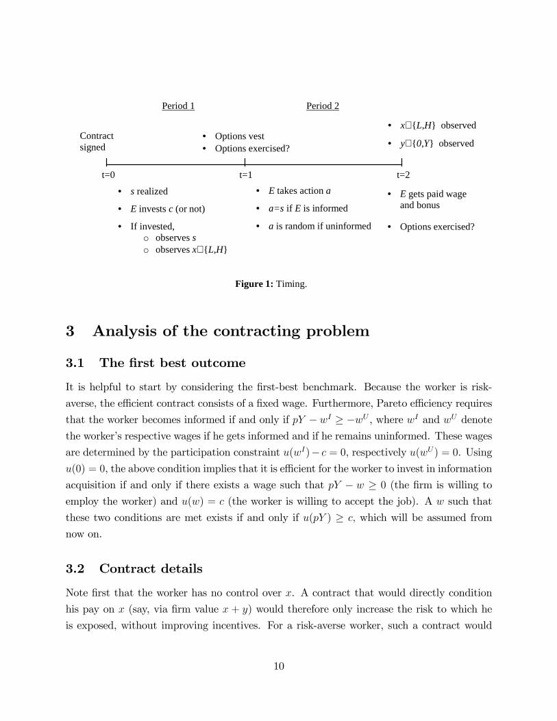
Timing. The model unfolds in three stages, as illustrated in Figure 1 below. (In thefigure, E stands for “employee.”)

At date 0, the firm and the worker sign an employment contract. Subsequently, the state

of the world s is realized and the worker decides whether to invest c in learning the state

and through it also the value of the firm’s assets.

At date 1, an informed worker chooses action a = s whereas an uninformed worker

chooses an action at random. The option grant vests and the worker can choose to exercise

his options (and sell the stock).

At date 2, both the value of the firm’s assets, x, and the realization of the worker’s

contribution to the firm’s value, y, are publicly revealed. The worker is paid his contingent

bonuses and decides whether to exercise his options if he has not done so at date 1.

6Assumption (iii) could be relaxed by introducing noise trading a la Kyle (1985), but this would onlycomplicate the analysis without changing the paper’s main insights. Alternatively, one could bypass thecomplications due to informed trading altogether, by assuming that the gains from option exercises aresettled in cash, as in Laux (2010).

9

Contractsigned

• x∈L,H observed

• y∈0,Y observed

• E gets paid wageand bonus

• Options exercised?

• s realized

• E invests c (or not)

• If invested,o observes so observes x∈L,H

• E takes action a

• a=s if E is informed

• a is random if uninformed

• Options vest• Options exercised?

Period 1 Period 2

t=0 t=1 t=2

Figure 1: Timing.

3 Analysis of the contracting problem

3.1 The first best outcome

It is helpful to start by considering the first-best benchmark. Because the worker is risk-

averse, the effi cient contract consists of a fixed wage. Furthermore, Pareto effi ciency requires

that the worker becomes informed if and only if pY − wI ≥ −wU , where wI and wU denotethe worker’s respective wages if he gets informed and if he remains uninformed. These wages

are determined by the participation constraint u(wI)− c = 0, respectively u(wU) = 0. Using

u(0) = 0, the above condition implies that it is effi cient for the worker to invest in information

acquisition if and only if there exists a wage such that pY − w ≥ 0 (the firm is willing to

employ the worker) and u(w) = c (the worker is willing to accept the job). A w such that

these two conditions are met exists if and only if u(pY ) ≥ c, which will be assumed from

now on.

3.2 Contract details

Note first that the worker has no control over x. A contract that would directly condition

his pay on x (say, via firm value x + y) would therefore only increase the risk to which he

is exposed, without improving incentives. For a risk-averse worker, such a contract would

10

be dominated by a contract that is independent of x. This is the essence of the arguments

against the use of employee stock options for incentive purposes.7

As will be shown below, in the current framework this argument does not imply that

using options to provide incentives is sub-optimal. It does imply, though, that the optimal

contract will not include a bonus directly contingent on x. It is therefore enough to restrict

attention to contracts that consist of (i) a base salary w0, (ii) a bonus b contingent on y :

b =

B when y = Y

0 when y = 0,

and (iii) a stock option grant on α shares of the firm, 0 ≤ α ≤ 1, with strike price K, where

the options vest at date t = 1.

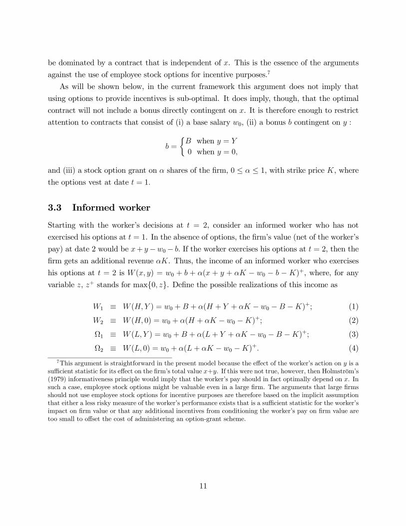
3.3 Informed worker

Starting with the worker’s decisions at t = 2, consider an informed worker who has not

exercised his options at t = 1. In the absence of options, the firm’s value (net of the worker’s

pay) at date 2 would be x+ y−w0− b. If the worker exercises his options at t = 2, then the

firm gets an additional revenue αK. Thus, the income of an informed worker who exercises

his options at t = 2 is W (x, y) = w0 + b + α(x + y + αK − w0 − b − K)+, where, for any

variable z, z+ stands for max0, z. Define the possible realizations of this income as

W1 ≡ W (H, Y ) = w0 +B + α(H + Y + αK − w0 −B −K)+; (1)

W2 ≡ W (H, 0) = w0 + α(H + αK − w0 −K)+; (2)

Ω1 ≡ W (L, Y ) = w0 +B + α(L+ Y + αK − w0 −B −K)+; (3)

Ω2 ≡ W (L, 0) = w0 + α(L+ αK − w0 −K)+. (4)

7This argument is straightforward in the present model because the effect of the worker’s action on y is asuffi cient statistic for its effect on the firm’s total value x+y. If this were not true, however, then Holmström’s(1979) informativeness principle would imply that the worker’s pay should in fact optimally depend on x. Insuch a case, employee stock options might be valuable even in a large firm. The arguments that large firmsshould not use employee stock options for incentive purposes are therefore based on the implicit assumptionthat either a less risky measure of the worker’s performance exists that is a suffi cient statistic for the worker’simpact on firm value or that any additional incentives from conditioning the worker’s pay on firm value aretoo small to offset the cost of administering an option-grant scheme.

11

After he learns the value of the firm’s assets, this worker’s expected utility is thus

EU Inf2 (H) = pu(W1) + (1− p)u(W2) if x = H

and EU Inf2 (L) = pu(Ω1) + (1− p)u(Ω2) if x = L.

What would the worker’s expected utility be if he instead exercised his options at t = 1

(or not at all)?8 Suppose the investors believe the worker is informed. Then they expect

the firm’s revenue to be L + q4 + pY + δαS, where δ is their belief about the probability

with which the worker will exercise his options at some point. Although the investors do

not observe the worker’s trading choices, they realize that he will trade based on his private

information, which will result in an expected loss to them of `(α), the exact expression for

which will be determined shortly. The (1− α) shares retained by the investors are therefore

worth to them

Eπ = (1− δ) [L+ q4+ p (Y −B)− w0]+δ (1− α) [L+ q4+ p (Y −B)− w0 + αK]−`(α).

(5)

Thus, if the worker exercises his options at t = 1, he can sell each share for the price of

P1 =Eπ

1− α. (6)

The income of an informed worker who exercises his options at t = 1 is therefore w0 + b +

α (P1 −K)+ and his expected utility is

EU Inf1 = pu(W3) + (1− p)u(W4)

for both x = H and x = L, where

W3 ≡ w0 +B + α (P1 −K)+ and W4 ≡ w0 + α (P1 −K)+ . (7)

The following proposition describes the informed worker’s optimal trading strategy.

Proposition 1. Let C∗ ≡ (w∗0, B∗, α∗, K∗) denote an optimal contract and suppose it

includes employee stock options (i.e., α∗ > 0). Under C∗, an informed worker exercises

his options as follows: When x = L, the worker exercises his options at t = 1. When

8After exercising his options at t = 1, the worker could hold on to his shares for a period and then sellthem in t = 2. This strategy, however, is payoff equivalent to exercising the options at t = 2 and willtherefore be ignored.

12

x = H and y = Y , he exercises his options at t = 2. When x = H and y = 0, he may

or may not exercise his options, but if he does, he does so at t = 2.

The logic behind Proposition 1 is that because options impose risk on the worker, it

makes sense to include them in the contract only if they provide incentives; otherwise, a

bonus contract without an option grant would provide the same incentives at a lower ex-

pected wage cost. But options provide incentives only if the worker conditions their exercise

on the realization of x; otherwise, an uninformed worker could replicate an informed worker’s

trading strategy, which would eliminate the worker’s incentive to invest in information ac-

quisition. Hence, the option grant must be structured so that when x = L, the worker wants

to take advantage of his private information and sell his stock at t = 1, before other investors

learn that the value of the firm’s assets is low. When x = H, the worker waits until t = 2,

when the good news gets incorporated in the price of the shares.

Given the worker’s trading strategy described in Proposition 1, the expected utility of an

informed worker under an optimal contract that includes an option grant can be written as

EU Inf = qEU Inf2 (H) + (1− q)EU Inf1

=

Exercise in t=2

q︷ ︸︸ ︷[pu(W1) + (1− p)u(W2)] + (1− q)

Exercise in t=1︷ ︸︸ ︷[pu(W3) + (1− p)u(W4)]

3.4 Firm’s expected payoff

The arguments behind Proposition 1, which rely on the option grant being valuable only if

it provides incentives, are not enough to restrict the worker’s decision regarding the exercise

of his options when x = H and y = 0. To streamline the exposition, the subsequent analysis

will focus on the case where K is suffi ciently low so that exercising the options is always

optimal, even when y = 0. Given the goals of the analysis, this restriction is harmless —if

the strike price in the option grant studied here is suboptimal but the principal nevertheless

finds it profitable to include the grant in the worker’s contract, then she would surely find

it optimal to include an option grant that is structured optimally. Similarly, any desirable

effi ciency properties of a potentially suboptimal option grant must also carry over to the

case of an optimally designed option grant.

Proceeding under the assumption that the worker always exercises his options (δ = 1)

13

the investors’expected payoff (5) becomes

Eπ = q (1− α) [H + p (Y −B) + αK − w0] + (1− q) [L+ p (Y −B) + αK − w0 − αP1]= (1− α) [L+ q4+ αK + p (Y −B)− w0]−α (1− q) [P1 − (L+ αK + p (Y −B)− w0)] . (8)

This expression is simple to understand. The second line says that the investors keep the

share 1−α of the firm’s expected revenues net of the worker’s wage and expected bonus, whilethe term `(α) ≡ α (1− q) [P1 − (L+ p (Y −B) + αK − w0)] in the third line represents theexpected loss the firm’s owners incur because the worker trades on his private information.

Of course, while `(α) is a loss for the investors, it represents a gain for the worker and the

prospect of this gain motivates him to become informed. The initial owners understand this

and purposefully incorporate this gain/loss into the contract in the design stage.

Returning to the first period stock price, plugging (8) into (6) yields

P1 = L+ q4+ αK + p (Y −B)− w0 −α

1− α (1− q) [P1 − (L+ αK + p (Y −B)− w0)] ,

from which one can solve for the price as

P1 = L+ q4+ αK + p (Y −B)− w0 −αq (1− q)

1− αq 4. (9)

The first period price is thus equal to the firm’s expected value, L+q4+αK+p (Y −B)−w0, minus the expected loss per share,

αq(1−q)1−αq 4, that is due to the worker’s informed trading

at t = 1 when x = L. The worker takes advantage of his private information by exercising

his options early when he learns that the state is bad, x = L. Intuitively, the investors’

loss is thus proportional to the number of options held by the worker (α), to the difference

between the expected value of the firm’s assets and their true (low) value when the worker

takes advantage of his private information (L + q4 − L), and to the probability that the

worker will get a chance to take advantage of his private information (1− q).

3.5 Uninformed worker

Now consider an uninformed worker. The probability that the worker correctly guesses the

exact state s is zero; accordingly, an uninformed worker never receives the bonus B. Will

this worker exercise his options at date 1 or at date 2? By assumption, the optimal contract

14

motivates the worker to become informed. Investors will therefore expect the worker to

be informed and hence, at t = 1, they will value the firm’s stock at P1. Therefore, if the

uninformed worker exercises his options at date 1, his payoff is

EUUninf1 = u(w0 + α(P1 −K)+) = u(W4). (10)

If, on the other hand, he exercises his options at t = 2, after x and y have been publicly

observed, his expected utility is

EUUninf2 = qu(w0 + α(H + αK − w0 −K)+) + (1− q)u(w0 + α(L+ αK − w0 −K)+)

= qu(W2) + (1− q)u(Ω2) (11)

Now, by Proposition 1, an informed worker who observes x = L is better off exercising his

options at t = 1 than not exercising them at all. It therefore has to be P1 > K under the

optimal contract. Thus, an uninformed worker, too, can benefit from exercising his options

at t = 1. The question is whether the worker prefers to wait until t = 2 or to exercise at t = 1.

Unfortunately, a priori, it is not possible to rule out either of these trading strategies. If the

first-period stock price P1 is suffi ciently depressed by the per-share lossαq(1−q)1−αq 4 expected

by the investors, then the worker is better off exercising his options at t = 1; otherwise,

waiting until t = 2 is optimal. Thus, in general, an uninformed worker exercises his options

at t = 1 if EUUninf1 ≥ EUUninf2 and at t = 2 if the opposite is true, and the analysis will have

to account for both possibilities.

3.6 Firm’s problem

If the firm decides to induce information acquisition, its optimal contract solves

maxw0,B≥0,α≥0,K≥0

Eπ (P)

subject to EU Inf − c ≥ maxEUUninf1 , EUUninf2 ; (12)

EU Inf − c ≥ 0, (13)

where (12) and (13) are the worker’s incentive compatibility and participation constraints

respectively.

The following proposition offers a partial characterization of the optimal option grant,

15

which will be helpful in the subsequent analysis of the owners’optimal contracting prob-

lem and in the characterization of the effi ciency properties of stock options in motivating

information acquisition.

Proposition 2. If the contract includes a stock option grant under which the worker alwaysexercises his options, then it is optimal to set the strike price such that L−w0

1−α ≤ K < P1.

Proposition 2 narrows down the range of possible strike prices that need to be considered

in the analysis of the optimal option grant. In particular, it shows that at the time of the

grant, the options will be in the money (K < P1), which we have already argued has to hold,

and that a grant of shares (K = 0) is weakly dominated by an option grant with a positive

strike price (K ≥ L−w01−α ).

The next proposition contains the first main result of this paper.

Proposition 3. If the principal finds it strictly profitable to induce information acquisition,then the optimal contract includes stock options, i.e., α∗ > 0.

Proposition 3 demonstrates that in the present model, it is always optimal to motivate

the worker by conditioning his pay on the value of the whole firm via a stock option grant.

This is true even though the worker’s contribution to firm value is observed and can be

contracted upon and even though the component of the firm value that is not affected by the

worker’s action is risky and does not contain any additional information about the worker’s

action. Note that these are precisely the conditions under which stock based compensation

has been considered puzzling.

The intuition for this result is as discussed earlier: An option contract induces the worker

to “get involved” in the firm by acquiring information that allows him to better estimate

the firm’s future value, which helps him to time his trading. The firm is willing to tolerate

the worker’s insider trading because his investment in firm-specific information makes him

more productive and thus more valuable to the firm.

4 Effi ciency properties of the option contract

How effi cient are options in motivating the worker? We have seen that the optimal incentive

contract will always include some options, but one may wonder whether the incentives that

come from the option part of the contract are of first order importance. In other words,

wouldn’t the option part disappear if administering an option grant entailed a small fixed

16

cost? This section shows that this is not the case; in fact, we will see that in some situations

options provide much more effective incentives than bonuses based on the worker’s individual

contribution to the firm value.

Under the standard theory, employee stock options are especially puzzling in large firms.

This is because in large firms the component of the firm’s value over which the employee has

no control is large and imposes on him large risk that is unrelated to his performance. The

purpose of the analysis below is to show that this logic does not apply in the present model.

In the model of this paper, the part of the variation in firm value that the worker cannot

affect is captured by the variance of the value of the firm’s assets, which is given by q(1−q)42.

A natural way to capture both the firm’s size and the magnitude of the risk unrelated to

the worker’s performance is thus through 4: For any given q, both the variance q(1− q)42

and the expected value of the assets, L + q4, are large if 4 is large.9 The first result

of this section will be that, contrary to the intuition based on the standard logic, in the

present framework stock options are especially effi cient when 4 is large. To demonstrate

this as simply as possible, the analysis will focus on the effi ciency properties of a pure bonus

contract and compare them with those of a pure option contract.

4.1 A pure bonus contract

A pure bonus contract is a contract that includes a bonus for y = H but does not contain

any options: B > 0 and α = 0. Given the assumption that the firm’s initial owners prefer to

induce the worker to get informed, their profit is maximized when information acquisition is

induced at the lowest possible wage cost. Thus, under a pure bonus contract the optimization

problem (P) can be written as

minw0,B≥0

(w0 + pB)

subject to pu(w0 +B) + (1− p)u(w0)− c ≥ u(w0);

pu(w0 +B) + (1− p)u(w0)− c ≥ 0.

The usual argument implies that both constraints must bind, so that u(w0) = 0 (from

which w0 = 0) and pu(B) = c, or B∗ = u−1(c/p). The firm’s expected wage bill is then

EWBonus = pu−1(c/p). (14)

9The effect of variance would be better isolated if the mean L+ q4 were kept constant. This, however,would necessitate allowing for a negative L, which would violate the limited liability property of stock.

17

4.2 A pure option contract

A pure option contract includes options but no bonus: α > 0 and B = 0. The analysis of

this contract is more complicated than the analysis of the bonus contract, and the details

are relegated to the proof of Proposition 4, but the core of the argument can be explained

relatively easily for the case where EUUninf1 ≥ EUUninf2 at the optimum. In this case, the

relevant incentive compatibility constraint in (12) is EU Inf − c ≥ EUUninf1 . Using W3 = W4

implied by B = 0, the firm’s optimization problem becomes

minw0,α≥0

q [pW1 + (1− p)W2] + (1− q)W3

subject to q [pu(W1) + (1− p)u(W2)] + (1− q)u(W3)− c ≥ u(W3); (15)

q [pu(W1) + (1− p)u(W2)] + (1− q)u(W3)− c ≥ 0. (16)

Again, both of the constraints must bind, which implies u(W3) = W3 = 0. The two

constraints thus collapse into a single constraint

q [pu(W1) + (1− p)u(W2)] = c. (17)

The firm’s expected wage bill under a pure option contract is then

EWOptions = q [pW1 + (1− p)W2] .

Recalling from (1) and (2) that W1 = W2 + αY and W2 = w0 + α(H + αK − w0 −K), this

can be written as

EWOptions = qW2 + qpαY. (18)

4.3 A comparison

A pure option contract is more effi cient than a pure bonus contract if EWOptions < EWBonus.

Now, to focus on large 4, let 4 → ∞. It will be shown in the proof of Proposition 4 thatα must then converge to zero, so that both W1 and W2 must approach some W . Condition

(17) therefore converges to

qu(W ) = c,

18

and the firm’s expected wage bill under a pure option contract (18) converges to

EWOptions = qW = qu−1(c/q). (19)

Observe that (19) has the same form as the bonus wage bill (14), with p replaced by q.

This makes sense: A pure bonus contract is conditioned on the realization of y, which is high

with probability p. In contrast, a pure option contract is conditioned predominantly on the

realization of x when 4 is very large (because y is negligible compared to x), which is high

with probability q.

Now, the expression zu−1(c/z) decreases in z. For large 4, a pure option contract istherefore more effi cient than a pure bonus contract (EWOptions < EWBonus) if and only

if q > p. The proof of Proposition 4 demonstrates that this conclusion continues to hold

when one allows for the possibility that EUUninf1 ≤ EUUninf2 at the optimum. The result is

summarized as follows.

Proposition 4. For any L and any q > p, there exists a finite 4 such that EWOptions <

EWBonus for all 4 ≥ 4. That is, if the variance and the expected value of the firm’sassets are suffi ciently large, a pure option contract exists that is more effi cient than the

optimal pure bonus contract.

Proposition 4 says that a pure option contract is often more effi cient than a pure bonus

contract, especially in large firms. But how much more effi cient? The next result shows

that the effi ciency difference between these two contracts can be vast. Because the worker is

risk averse and the firm’s value is risky, there of course exists no contract that can achieve

the first best outcome. Nevertheless, there are situations in which the outcome under an

option contract is arbitrarily close to the first best outcome, while a pure bonus contract is

so ineffi cient that the firm is better off not using it and letting the agent remain uninformed.

Let V FB denote the owners’expected payoffunder the first best scenario, i.e., when there

is no moral hazard problem. Similarly, define V Options to be the owners’expected payoff

under the optimal pure option contract.

Proposition 5. (i) Consider a pure bonus contract. For any p, there exist Y1 and Y2 suchthat when Y ∈ (Y1, Y2), the optimal contract sets B∗ = 0. Under this contract, the

worker remains uninformed, even though effi ciency requires that he get informed.

(ii) Consider a pure option contract. For any ε > 0, there exist q < 1 and 4 < ∞ such

that if q ≥ q and 4 ≥ 4, the effi ciency loss under the optimal contract is less than

19

ε, i.e., V FB − V Options < ε. In other words, for 4 and q large the option contract

approaches the first best outcome.

The result in part (i) of Proposition 5 is standard. Given the moral hazard problem, a

second best contract cannot achieve the first-best outcome. Furthermore, in situations where

the first-best surplus is relatively small to start with (which is the case when Y < Y2), a

second-best contract may not be effi cient enough to generate any surplus.

Part (ii) is more interesting. It says that a pure option contract can be very effi cient;

almost as effi cient as a first-best contract. Moreover, this effi ciency result does not depend on

the exact value of Y —it only requires that the potential increase in the value of the firm’s

assets, 4, and the probability q that the asset value is high are suffi ciently large. Thus,there are situations when an option grant is vastly more effi cient than a contract based on

the worker’s individual performance, even in a large firm.

5 Empirical implications

The theory developed above has implications for the kind of firms we should expect to use

employee stock options, for the relationship between firm size and the use of stock option

grants, for the optimal way to structure the vesting period of an option grant, and for the

relationship between option grants and employee turnover.

First, the model predicts that the incentive effects of employee stock options should be

valuable in firms that need to encourage their employees to invest in information, especially

firm-specific information. This prediction is consistent with the evidence that both the

likelihood and the intensity of the use of non-executive stock options are higher in firms in

which human capital is a relatively more important factor of production (Core and Guay,

2001; Kroumova and Sesil, 2006; Jones et al, 2006). It is also consistent with the evidence

that stock options are widespread in start-up firms: By default, all employees in a start-up

are new to the job and therefore unlikely to possess firm-specific human capital. Start-up

firms therefore tend to be more in need of motivating their employees to invest in firm-

specific information than are established and mature firms. Moreover, in mature firms, new

employees may need less of an incentive to invest in firm-specific knowledge because at least

some of the required knowledge will seep to them from their more senior co-workers and

from their supervisors. Young firms, not having workers with long tenure, cannot rely on

this “automatic”mechanism of information dissemination.

20

Second, firm size has an ambiguous effect on whether employee stock options are useful

for providing incentives. The usual free rider argument favors their use in small firms, but

benefits to informed trading may be easier to realize in large firms, in which a trade by any

single (lower level) employee is less likely to affect the stock price. Although the paper does

not directly model this tradeoff, it is not hard to see that the trade-off could be resolved in

favor of any firm size: If investment in firm-specific information is not very important relative

to the direct effect of the workers’effort on firm value, then in line with the traditional logic

a large firm will not use stock options. If, however, investment in firm-specific knowledge

is important and hiding informed trading becomes easier the larger is the firm, then the

incentive effects of employee stock options could well be most useful in medium to large

sized firms. Indeed, there is some evidence that larger firms are more likely to adopt broad

based share plans (Jones et al, 2006).

Third, the theory offers a new perspective on how the options’ vesting period affects

their incentive properties. While a proper investigation of this topic would require a more

dynamic model than the one studied in this paper, the basic issues that are at play here are

relatively transparent. Specifically, the length of the vesting period will influence the type

of information the employee will be willing to acquire. Options with a long vesting period,

for example, will not be effective in motivating the acquisition of short-lived information

whose relevance expires before the options vest. On the other hand, when the vesting period

is short, the option grant may not work well if information acquisition is important in the

time period after the options vest because by that time the worker may have exercised the

options, either for liquidity reasons or due to diversification reasons.

Finally, similar to Oyer (2004), the model has implications for the relationship between

stock options’use and employee turnover. In Oyer’s theory, the main role of options is to

prevent employee turnover; accordingly, we should expect that in the years following a broad-

based stock option grant, employee turnover falls at the granting firm. The theory developed

here has a similar implication: Since in the present model options serve to induce firm-

specific investments, they also affect the probability of turnover negatively, for the reasons

well known from the theory of firm-specific human capital. In this respect, both models

are consistent with the available empirical evidence, which indeed documents a negative

relationship between stock option grants and subsequent worker turnover (Aldatmaz, Ouimet

and Van Wesep, 2012).

There is one important aspect though in which the implications here differ from those

of Oyer (2004): Whereas in Oyer’s model the relationship between options and turnover

21

disappears after the vesting period, in the present model the relationship between vesting a

turnover is more complicated: On the one hand, some of the workers who were planning to

move may wait long enough for their options to vest, and then quit shortly afterwards. This

would increase the probability of turnover right after the vesting period. On the other hand,

as long as the firm-specific knowledge acquired by the workers remains relevant, it should

provide a disincentive to move even after the options vest. Thus, suppose we compare three

firms, A, B, and C. Firms A and B each adopt a broad-based option plan that vests, say,

in three years. In firm A, the options are used solely to manage turnover whereas in firm

B they serve to motivate investments in firm-specific knowledge. Firm C does not grant

options. In all other respects, the three firms are identical. Then comparing the aggregate

levels of turnover in the three firms over the period of, say, five years, we should see little

difference between firms A and C, whereas firm B (the one whose workers invest in firm-

specific knowledge), should exhibit a lower level of turnover over this period.

The above prediction is consistent with the findings in Bryson and Freeman (2013) who

use survey data from the UK establishments of a multinational firm to examine the effects of

a company subsidized employee stock purchase plan. Bryson and Freeman document that the

workers who choose to participate in the plan are subsequently less likely to leave or search

for a different job than those who do not participate in the plan. The UK tax laws offer a

substantial tax break for holding the shares for at least five years, so similar to the effects

of a vesting period for option grants, any negative relationship between plan participation

and turnover should disappear if the plan only affects the workers’participation constraints

but not their incentives, as in Oyer (2004). However, Bryson and Freeman show that even

the workers who have been participating in the plan for more than five years exhibit lower

probabilities of turnover. Bryson and Freeman’s interpretation is that the workers view the

subsidized shares as a gift and reciprocate it with better performance and a lower probability

of quitting. The present paper offers an alternative explanation, according to which the

share purchase plan motivates firm-specific investments by the workers, which in turn makes

it more costly for them to switch employers.

6 Discussion of assumptions

The model developed above assumes that the employment contract cannot be based on

messages from the worker to the firm and that the worker cannot trade company securities on

his own in the financial markets. This section provides a discussion of these two assumptions.

22

6.1 Contracting on messages

In the model of this paper, an option contract provides incentives because it conditions the

worker’s pay on his information about the state of the world. In principle, this could be

done more directly: at t = 1, the worker could make an announcement m ∈ L,H aboutthe future value of the firm’s assets and then receive a bonus if x = m. Being a more general

version of the option contract, such a message-based contract could always do at least as well

as the option contract. An option contract, however, may have advantages over a contract

based on messages:

First, the messages would have to be publicly verifiable. But for various strategic reasons,

a firm might not want its employees to make public predictions about the future of their

firm, especially if the news is negative. The firm could try and keep the predictions hidden

from the public eye, but given that someone would have to overlook such a scheme, it would

not be easy to ensure that the predictions are kept secret. Moreover, the scheme would be

enforceable only if a compliance with it could be verified in the court of law, which would

make secrecy even harder to achieve. In short, administering such a scheme seems impractical

and could well be costlier than administering an option grant.

Second, employees might free ride on each other’s predictions. They could, of course,

also free ride on each other’s trading strategies, but informed trading may be easier to hide —

and the workers would have an incentive to do so, in order to prevent imitators from moving

the stock price. Furthermore, workers may trade for reasons other than to take advantage

of private information; in particular, they may exercise their options to meet their liquidity

and consumption needs. If employees cannot distinguish between a co-worker’s motives for

trading, this would limit their benefits from free riding.

To sum up, compared to an option contract, a contract based on messages might be more

costly to implement, would leak more information to the firm’s competitors and investors, and

would require that the owners have more information about the details of the environment.

An option contract might thus be more practical, especially when, as shown in Proposition

5, its effi ciency is close to the first best benchmark.

6.2 Open market trading

The analysis of the model was conducted under the assumption that the worker cannot pur-

chase his company’s shares, options, and other derivatives in the open market. As mentioned

earlier, companies often prohibit their employees from short selling company stock and from

23

engaging in trades involving derivatives, such as put options on the firm’s stock.10 Neverthe-

less, workers are typically free to purchase shares of the company stock. Thus, in principle,

rather than granting him options, the firm could simply let the worker trade the firm’s stock

in the open market, which could be a profitable strategy for an informed worker.

There are at least two reasons firms may offer employee stock options even if open market

trading is feasible. First, although inside information may induce a risk-averse worker to

purchase more of his own company’s stock than suggested by traditional hedging arguments

(Van Nieuwerburgh and Veldkamp, 2006), it may not be enough from the firm’s perspective.

This is because the worker only takes into account his private benefit from getting informed

and does not internalize the resulting increase in the firm’s profit. Proposition 6 below

formalizes this logic.

Proposition 6. Suppose that at t = 1 the worker can purchase the firm’s shares on the

open market. There exist q+ < 1, 4+ <∞, and a non-empty interval (Y −, Y +) such

that if q ≥ q+, 4 ≥ 4+, and Y ∈ (Y −, Y +), the optimal contract includes an option

grant (i.e., α∗ > 0).

Proposition 6 says that the firm may find it optimal to include an option grant in the

worker’s incentive contract even if the worker is able to trade in the financial markets.

Although the result is likely to hold for a broader range of parameter values, for tractability

purposes the proposition focuses on parameter values such that q and 4 are large and Y

is in an intermediate range. These are also the parameter values for which the intuition

behind the result is most transparent: We know from Proposition 5 that when Y ∈ (Y1, Y2),

incentives provided by a pure bonus contract (with no open market trading) are so costly

that the firm opts to provide no incentives even though effi ciency requires that the worker

get informed. The proof of Proposition 6 shows that when q is close to 1, allowing for open

market trading does not alter this qualitative conclusion: There again exists a range of Y ,

given by the interval (Y −, Y +), such that in the absence of an option grant the worker does

not (always) get informed.11 This is because the stock price reflects the expected average

asset value qH + (1− q)L, which is close to H when q is close to 1. The potential gain from

10Benefits to such restrictions are outside of this model, but statements of real world firms’insider tradingpolicies indicate that firms implement the restrictions because they worry an employee who shorts thecompany stock, or holds puts on it, would benefit from a decrease in the stock price, which might provideher with perverse incentives. Note that employee stock options do not suffer from this problem.In addition, firms worry that trading in puts or other hedging instruments might be interpreted as a

negative signal to the market that the employee has no confidence in the company’s prospects. This alsoapplies to exercising call options, but to a lesser extent.11The worker may choose to randomize in his decision to get informed because the positive probability

24

buying the firm’s stock when the asset value is H is therefore minuscule, so that it would be

worth getting informed only if the worker expected to purchase a relatively large number of

shares. However, a risk-averse worker is reluctant to buy a large number of shares because

of the risk associated with the realization of his marginal contribution y. Thus, in this case

open market trading is not enough to always induce the worker to get informed, even if

combined with a bonus contract. On the other hand, Proposition 5 tells us that when q is

close to 1 and 4 is large, an option contract is almost fully effi cient. Thus, the firm would

want to motivate the worker with an option grant.

The second reason why open market trading may not provide suffi cient incentives is that

the worker may face a wealth constraint and therefore may not be able to purchase (enough)

shares of the firm’s stock. This assumption is often adopted in the literature on insider

trading (e.g., Dye, 1984; Noe, 1997; Laux, 2010). Of course, a wealth constraint changes

other aspects of the analysis as well; in particular, it makes it harder for the firm to extract

from the worker his expected gains from informed trading. It is therefore not immediate that

an option grant would remain optimal if the worker were liquidity constrained. The next

proposition establishes that the conclusion of Proposition 3 continues to hold even when the

worker is liquidity constrained and hence unable to trade in the open market.

Proposition 7. Suppose the worker is liquidity constrained in the sense that his pay cannotbe negative. Then if the principal finds it strictly profitable to induce information

acquisition, the optimal contract always includes stock options, i.e., α∗ > 0.

To sum up, although open market trading could provide the worker with some incentives

to get informed, in general it is not a good substitute for including an option grant in the

worker’s contract.

7 Conclusion

This paper has argued that, contrary to the prevalent view among economists, the observa-

tion that large firms suffer from severe free rider problems is not suffi cient to rule out stock

option plans as effective incentive tools for lower level employees. The free rider critique is

predicated upon the assumption that a worker can be motivated by stock-based compen-

sation only to the extent that her actions increase the value of the firm’s shares, an effect

that the worker is uninformed depresses the equilibrium stock price P1 and increases the worker’s tradinggain when he does get informed. The proof of the proposition allows for such a mixed strategy.

25

that for a typical worker is indeed minuscule in large firms. However, by the very nature

of stock options, a worker can increase their value not only by increasing the value of the

firm but also by simply getting informed about the details of the firm’s operations. Unlike

the standard free rider problem, this effect is not directly related to the size of the firm

and therefore can be of significant magnitude even in large firms. Consequently, the paper

demonstrates that if the firm’s goal is to encourage investments by workers in firm-specific

information, broad-based stock option grants may be an effective way to do this. Moreover,

under some conditions, options can provide significantly more effi cient incentives than even

performance contracts based on the worker’s individual contribution to the firm value.

The theory developed in this paper has potentially testable empirical implications. For

example, the use of employee stock options for incentive purposes should be observed mainly

in firms that need to encourage their employees to accumulate firm-specific knowledge, such

as high tech firms and start-ups. Also, firms that use broad based stock option grants

should exhibit less employee turnover, even over periods that exceed the duration of the

vesting period.

The basic model examined in this paper could be extended in several directions. Perhaps

the most promising avenue for further study would be to endogenize the vesting period. Such

a framework could then be used to address the open question of what determines the length

of the optimal vesting period and to study the relationship between an optimal vesting policy

and the nature of the specific information (e.g., long-lived vs short-lived) that the firm wants

the workers to accumulate.

A Appendix: Proofs

Proof of Proposition 1. Step 1. Observe first that if α∗ > 0, then the options must provide

incentives, i.e., it must be that under the contract C∗ the worker gets informed, whereas under

the contract C0 ≡ (w∗0, B∗, α = 0) he would find it optimal to stay uninformed. If this were

not the case, then there would be an alternative contract C ′ = (w0, B∗, α = 0) that would

dominate C∗, because C ′ could provide the same level of incentives as C∗ without imposing

on the worker the additional risk due to the variations in x.

Step 2. Given that the stock option part of C∗ provides incentives, it must be that an

informed worker conditions his trading on his private information. Moreover, it cannot be

that he never exercises his options at t = 1, regardless of his private information. If this were

the case, the options would not provide any incentives because the worker could replicate

26

this trading strategy even without getting informed – he could simply wait until the firm’s

revenue is publicly observed at t = 2 and then exercise his options optimally. Similarly, it

cannot be that in equilibrium an informed worker never exercises his options at t = 2. In

such a case, the worker would exercise his options at t = 1 iffK < P1. But this rule does not

depend on the exact realization of x, so an uninformed worker could replicate this trading

strategy. Once again, the options would not provide any incentive to get informed.

Step 3. The previous step leaves three possible cases for an informed worker’s equilibrium

trading strategy:

(i) If x = L, exercise at t = 1; if x = H, exercise at t = 2, either for y = Y , or for both

realizations of y.

(ii) If x = H, exercise at t = 1; if x = L, then exercise at t = 2, but only if y = Y .

(iii) If x = H, exercise at t = 1; if x = L, exercise at t = 2 for both realizations of y.12

The proof is concluded by ruling out (ii) and (iii). Start with (iii): If at t = 2 it is publicly

revealed that x = L, the stock price must (in expectation with respect to y) decrease from

what it was at t = 1. Hence, if the worker finds it optimal to exercise his options at t = 2

when x = L, it must be even better to exercise them at t = 1, because not only is his payoff

higher in expectation (due to the higher stock price), but it is also less variable (due to the

realization of y in t = 2), which the risk-averse worker likes. As for case (ii), note that when

x = L, any realization of the stock price at t = 2 must always be lower than the stock price

at t = 1. The reason is that at t = 1, the price reflects the expected value of x+ y as given

by L + q4 + pY , but when it is revealed at t = 2 that x = L, the price must fall because,

by assumption, q4 > (1− p)Y . Thus, when x = L, the worker strictly prefers exercising his

options at t = 1 to exercising them at t = 2, which rules out case (iii). Q.E.D.

Proof of Proposition 2. As pointed out in the text, the fact that K < P1 follows from

Proposition 1, which says that the informed worker always finds it optimal to exercise his

options at t = 1 if x = L. Thus, it remains to prove that K ≥ L−w01−α .

Given the assumption that the firm’s initial investors prefer to induce the worker to get

informed, their optimization problem (P) can be reduced to the problem of minimizing the

expected cost of inducing the worker to get informed:

minw0,α≥0,B≥0,K≥0

q [pW1 + (1− p)W2] + (1− q) [pW3 + (1− p)W4]

12The cases where the worker exercises his options in t = 2 when y = 0 but not when y = Y are ruled outimmediately.

27

s.t. EU Inf ≡ q [pu(W1) + (1− p)u(W2)] + (1− q) [pu(W3) + (1− p)u(W4)]− c≥ qu(W2) + (1− q)u(Ω2) ≡ EUUninf2 ;

EU Inf ≡ q [pu(W1) + (1− p)u(W2)]+(1− q) [pu(W3) + (1− p)u(W4)]−c ≥ u(W4) ≡ EUUninf1 ;

and EU Inf ≡ q [pu(W1) + (1− p)u(W2)]+(1− q) [pu(W3) + (1− p)u(W4)]−c = 0.

Suppose K < L−w01−α . Given that the firm’s value at t = 2 is never less than L+αK −w0,

under this strike price the worker always exercises his options. Thus, the worker’s possible

incomes (originally given by (1)-(4) and (7)) and the first period price (9) can be written as

W1 = Ω2 +B + α(4+ Y −B); (A1)

W2 = Ω2 + α4; (A2)

W3 = Ω2 +B + α

(q4+ p (Y −B)− αq (1− q)

1− αq 4)

; (A3)

W4 = Ω2 + α

(q4+ p (Y −B)− αq (1− q)

1− αq 4)

; (A4)

Ω2 = αL+ (1− α) (w0 − αK) ; (A5)

P1 = L+ q4+ αK + p (Y −B)− w0 −αq (1− q)

1− αq 4. (A6)

Now, consider the effects of an increase in K to K ′ accompanied by an increase in w0to w′0 so that Ω2 remains unchanged and K ′ ≤ L−w′0

1−α . Given that K and w0 enter Ω2 only

through the term (w0 − αK), such an offsetting change in K and w0 is always possible.

Moreover, the worker’s income vector (W1,W2,W3,W4) depends on K and w0 only through

Ω2. This increase in K therefore has no effect on (W1,W2,W3,W4) and hence no effect on

the optimization problem. Consequently, K = L−w01−α must be at least as profitable for the

owners as any K < L−w01−α . Q.E.D.

Proof of Proposition 3. Given the result of Proposition 2, it is without loss of generalityto restrict attention to strike prices such that L−w0

1−α ≤ K < P1. Furthermore, for the purposes

of this proposition, one can set K = L−w01−α because if the optimal contract includes stock

options under this strike price, then it must also include stock options under the optimal

strike price, even if the optimal strike price differs from L−w01−α .

Thus, setting K = L−w01−α , the optimization problem specified in the proof of Proposition

28

2 simplifies to

minw0,α≥0,B≥0

q [pW1 + (1− p)W2] + (1− q) [pW3 + (1− p)W4]

s.t. EU Inf ≡ q [pu(W1) + (1− p)u(W2)] + (1− q) [pu(W3) + (1− p)u(W4)]− c≥ qu(W2) + (1− q)u(w0) ≡ EUUninf2 ;

EU Inf ≡ q [pu(W1) + (1− p)u(W2)]+(1− q) [pu(W3) + (1− p)u(W4)]−c ≥ u(W4) ≡ EUUninf1 ;

and EU Inf ≡ q [pu(W1) + (1− p)u(W2)]+(1− q) [pu(W3) + (1− p)u(W4)]−c = 0,

where W1 = w0 +B + α(4+ Y −B);

W2 = w0 + α4;

W3 = w0 +B + α

(q4+ p (Y −B)− αq (1− q)

1− αq 4)

;

W4 = w0 + α

(q4+ p (Y −B)− αq (1− q)

1− αq 4).

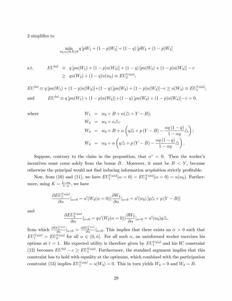
Suppose, contrary to the claim in the proposition, that α∗ = 0. Then the worker’s

incentives must come solely from the bonus B. Moreover, it must be B < Y , because

otherwise the principal would not find inducing information acquisition strictly profitable.

Now, from (10) and (11), we have EUUninf1 (α = 0) = EUUninf2 (α = 0) = u(w0). Further-

more, using K = L−w01−α , we have

∂EUUninf1

∂α|α=0 = u′(W4(α = 0))

∂W4

∂α|α=0 = u′(w0) [q4+ p (Y −B)]

and∂EUUninf2

∂α|α=0 = qu′(W2(α = 0))

∂W2

∂α|α=0 = u′(w0)q4,

from which ∂EUUninf1

∂α|α=0 > ∂EUUninf2

∂α|α=0. This implies that there exists an α > 0 such that

EUUninf1 > EUUninf2 for all α ∈ (0, α]. For all such α, an uninformed worker exercises his

options at t = 1. His expected utility is therefore given by EUUninf1 and his IC constraint

(12) becomes EU Inf − c ≥ EUUninf1 . Furthermore, the standard argument implies that this

constraint has to hold with equality at the optimum, which combined with the participation

constraint (13) implies EUUninf1 = u(W4) = 0. This in turn yields W4 = 0 and W3 = B.

29

Restricting attention to α ≤ α, the firm’s optimization problem can thus be written as

minw0,α≥0,B≥0

q [pW1 + (1− p)W2] + (1− q) pB

s.t. q [pu(W1) + (1− p)u(W2)] + (1− q) pu(B)− c = 0; (A7)

w0 + α

(q4+ p (Y −B)− αq (1− q)

1− αq 4)

= 0, (A8)

where W1 = w0 +B + α(4+ Y −B);

W2 = w0 + α4;

W3 = w0 +B + α

(q4+ p (Y −B)− αq (1− q)

1− αq 4).

Let λ and µ be the Lagrange multipliers that go with constraints (A7) and (A8) respectively.

The corresponding first order conditions are then

α : qp(4+ Y −B) [1 + λu′(W1)] + q(1− p)4 [1 + λu′(W2)]

+ µ

[q4+ p (Y −B)− α (2− αq)

(1− αq)2q (1− q)4

]≥ 0;

B : qp∂W1

∂B+ (1− q) p+ λ

[qpu′(W1)

∂W1

∂B+ (1− q) pu′(B)

]− µαp ≥ 0;

w0 : q + λ [qpu′(W1) + q(1− p)u′(W2)] + µ = 0.

Suppose B = α = 0. Then the contract provides no incentives, which means that (12)

cannot hold. Hence, if α = 0, then B > 0. Consequently, FOC(B) must hold with equality.

Now, evaluating at α = 0, we get W1 = W3 = w0 + B and W2 = W4 = w0, and, from

(A8), w0 = 0, so that the above first order conditions reduce to

α : qp(4+ Y −B) [1 + λu′(B)] + q(1− p)4 [1 + λu′(0)] + µ [q4+ p (Y −B)] ≥ 0; (A9)

B : 1 + λu′(B) = 0; (A10)

w0 : q [1 + λ [pu′(B) + (1− p)u′(0)]] + µ = 0. (A11)

Using (A10), condition (A9) becomes

α : q(1− p)4 [1 + λu′(0)] + µ [q4+ p (Y −B)] ≥ 0. (A12)

30

Now, (A10) implies λ < 0. Given that u′(0) > u′(B) (by concavity of u), (A10) yields

1 + λu′(0) < 0. Similarly, pu′(B) + (1 − p)u′(0) < u′(B) together with (A10) yields 1 +

λ [pu′(B) + (1− p)u′(0)] > 0, which combined with (A11) implies µ < 0. It must therefore

be LHS(A12) < 0, which contradicts (A12). Hence, it cannot be that α∗ = 0, which implies

α∗ > 0. Q.E.D.

Proof of Proposition 4. The analysis of the pure bonus contract was completed in thetext, so consider a pure option contract.

Step 1. Let B = 0 and set K = L−w01−α (which, as already argued earlier, can be done

without loss of generality given the goals of the analysis). (A1) - (A6) then yield

W1 = w0 + α(4+ Y );

W2 = w0 + α4;

W3 = W4 = w0 + α

(pY +

1− α1− αqq4

)Ω2 = w0.

Using (9), the expected utilities (10) and (11) can be written as

EUUninf1 = u

(w0 + α

(q4+ pY − αq (1− q)

1− αq 4))

;

EUUninf2 = qu(w0 + α4) + (1− q)u(w0).

Start with the case where EUUninf1 ≥ EUUninf2 at the optimum, so that the relevant incen-

tive compatibility constraint is EU Inf − c ≥ EUUninf1 . As mentioned in the text, constraints

(15) and (16) must both bind, from which u(W3) = W3 = 0. This holds if

w0 = −α(pY +

1− α1− αqq4

).

It then follows that the option grant α and the equilibrium incomes W1 and W2 satisfy

W1 = α

[1− q

1− αq4+ (1− p)Y], (A13)

W2 = α

(1− q

1− αq4− pY), (A14)

q [pu(W1) + (1− p)u(W2)] = c, (A15)

31

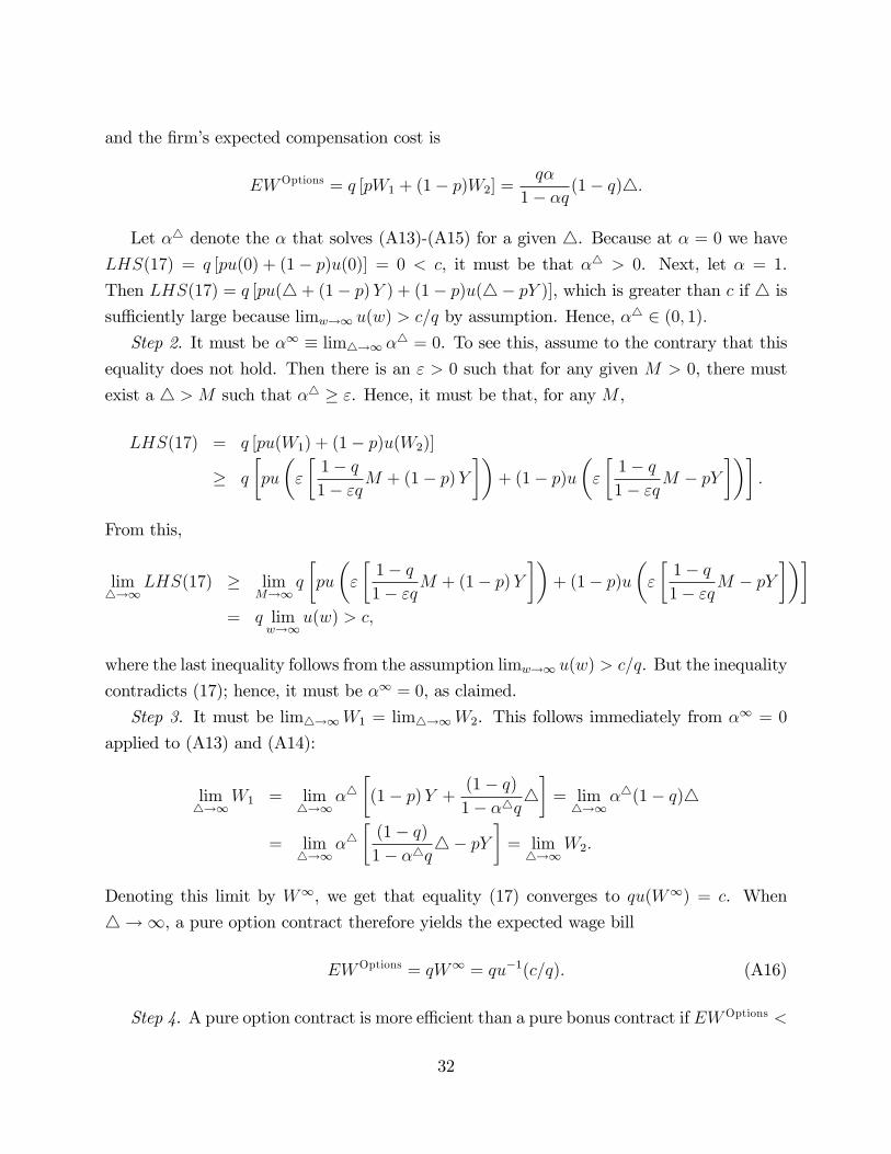
and the firm’s expected compensation cost is

EWOptions = q [pW1 + (1− p)W2] =qα

1− αq (1− q)4.

Let α4 denote the α that solves (A13)-(A15) for a given 4. Because at α = 0 we have

LHS(17) = q [pu(0) + (1− p)u(0)] = 0 < c, it must be that α4 > 0. Next, let α = 1.

Then LHS(17) = q [pu(4+ (1− p)Y ) + (1− p)u(4− pY )], which is greater than c if 4 is

suffi ciently large because limw→∞ u(w) > c/q by assumption. Hence, α4 ∈ (0, 1).

Step 2. It must be α∞ ≡ lim4→∞ α4 = 0. To see this, assume to the contrary that this

equality does not hold. Then there is an ε > 0 such that for any given M > 0, there must

exist a 4 > M such that α4 ≥ ε. Hence, it must be that, for any M ,

LHS(17) = q [pu(W1) + (1− p)u(W2)]

≥ q

[pu

(ε

[1− q1− εqM + (1− p)Y

])+ (1− p)u

(ε

[1− q1− εqM − pY

])].

From this,

lim4→∞

LHS(17) ≥ limM→∞

q

[pu

(ε

[1− q1− εqM + (1− p)Y

])+ (1− p)u

(ε

[1− q1− εqM − pY

])]= q lim

w→∞u(w) > c,

where the last inequality follows from the assumption limw→∞ u(w) > c/q. But the inequality

contradicts (17); hence, it must be α∞ = 0, as claimed.

Step 3. It must be lim4→∞W1 = lim4→∞W2. This follows immediately from α∞ = 0

applied to (A13) and (A14):

lim4→∞

W1 = lim4→∞

α4[(1− p)Y +

(1− q)1− α4q4

]= lim4→∞

α4(1− q)4

= lim4→∞

α4[

(1− q)1− α4q4− pY

]= lim4→∞

W2.

Denoting this limit by W∞, we get that equality (17) converges to qu(W∞) = c. When

4→∞, a pure option contract therefore yields the expected wage bill

EWOptions = qW∞ = qu−1(c/q). (A16)

Step 4. A pure option contract is more effi cient than a pure bonus contract if EWOptions <

32

EWBonus. For q > p and large 4, a comparison of (A16) and (14) reveals that this conditionholds if zu−1(c/z) decreases in z. Using ∂u−1(z)

∂z= 1

u′(u−1(z)) , this is true if and only if

u−1(c/z)u′(u−1(c/z)

)<c

z.

Let u−1(c/z) = W . Then the above condition can be rewritten as Wu′(W ) < u(W ), which

always holds because u(.) is strictly concave. Hence, in this case EWOptions < EWBonus if

q > p and if 4 is suffi ciently large.

Step 5. If EUUninf1 ≤ EUUninf2 at the optimum, it must be W3 ≤ 0. To see this, note that

in this case (12) becomes EU Inf − c ≥ EUUninf2 , so that the firm’s constraints are

q [pu(W1) + (1− p)u(W2)] + (1− q)u(W3)− c ≥ qu(W2) + (1− q)u(w0);

q [pu(W1) + (1− p)u(W2)] + (1− q)u(W3)− c ≥ 0.

Again, both of these constraints must bind, which implies

EUUninf2 = qu(W2) + (1− q)u(w0) = 0; (A17)

EU Inf = q [pu(W1) + (1− p)u(W2)] + (1− q)u(W3) = c. (A18)

Now, using (10) and W3 = W4 (from Step 1), we have EUUninf1 = u(W3). Thus, EUUninf1 ≤EUUninf2 combined with (A17) yields u(W3) ≤ 0,which implies W3 ≤ 0.

Step 6. It must be that lim4→∞ α∗ = 0. To obtain this claim, rewrite the firm’s opti-

mization problem using the expressions for W1, W2, W3, and Ω2 introduced in Step 1:

minw0≥0,α≥0

w0 + pαY + qα4+ q (1− q)α 1− α1− αq4

subject to qu(w0 + α4) + (1− q)u(w0) = 0; (A19)

and q [pu(w0 + α(4+ Y )) + (1− p)u(w0 + α4)]

+ (1− q)u(w0 + α

(pY +

1− α1− αqq4

))= c. (A20)

Observe first that it must be lim4→∞w0 > −∞. Otherwise, given that limw→∞ u(w) =

u < ∞ and limw→−∞ u(w) = −∞ (where the latter is implied by the assumption that

limw→−∞ u′(w) = ∞), the left hand side of (A19) would converge to −∞ and (A19) would

33

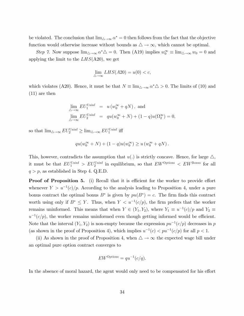
be violated. The conclusion that lim4→∞ α∗ = 0 then follows from the fact that the objective

function would otherwise increase without bounds as 4→∞, which cannot be optimal.Step 7. Now suppose lim4→∞ α

∗4 = 0. Then (A19) implies w∞0 ≡ lim4→∞w0 = 0 and

applying the limit to the LHS(A20), we get

lim4→∞

LHS(A20) = u(0) < c,

which violates (A20). Hence, it must be that N ≡ lim4→∞ α∗4 > 0. The limits of (10) and

(11) are then

lim4→∞

EUUninf1 = u (w∞0 + qN) , and

lim4→∞

EUUninf2 = qu(w∞0 +N) + (1− q)u(Ω∞2 ) = 0,

so that lim4→∞EUUninf2 ≥ lim4→∞EU

Uninf1 iff

qu(w∞0 +N) + (1− q)u(w∞0 ) ≥ u (w∞0 + qN) .

This, however, contradicts the assumption that u(.) is strictly concave. Hence, for large 4,it must be that EUUninf1 > EUUninf2 in equilibrium, so that EWOptions < EWBonus for all

q > p, as established in Step 4. Q.E.D.

Proof of Proposition 5. (i) Recall that it is effi cient for the worker to provide effort

whenever Y > u−1(c)/p. According to the analysis leading to Proposition 4, under a pure

bonus contract the optimal bonus B∗ is given by pu(B∗) = c. The firm finds this contract

worth using only if B∗ ≤ Y . Thus, when Y < u−1(c/p), the firm prefers that the worker

remains uninformed. This means that when Y ∈ (Y1, Y2), where Y1 ≡ u−1(c)/p and Y2 ≡u−1(c/p), the worker remains uninformed even though getting informed would be effi cient.

Note that the interval (Y1, Y2) is non-empty because the expression pu−1(c/p) decreases in p

(as shown in the proof of Proposition 4), which implies u−1(c) < pu−1(c/p) for all p < 1.

(ii) As shown in the proof of Proposition 4, when 4 →∞ the expected wage bill under

an optimal pure option contract converges to

EWOptions = qu−1(c/q).

In the absence of moral hazard, the agent would only need to be compensated for his effort

34

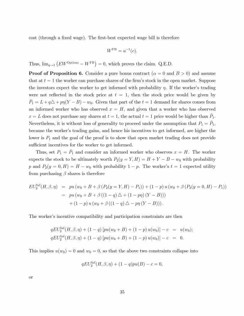
cost (through a fixed wage). The first-best expected wage bill is therefore

W FB = u−1(c).

Thus, limq→1(EWOptions −W FB

)= 0, which proves the claim. Q.E.D.

Proof of Proposition 6. Consider a pure bonus contract (α = 0 and B > 0) and assume

that at t = 1 the worker can purchase shares of the firm’s stock in the open market. Suppose

the investors expect the worker to get informed with probability η. If the worker’s trading

were not reflected in the stock price at t = 1, then the stock price would be given by

P1 = L+ q4+ pη(Y −B)−w0. Given that part of the t = 1 demand for shares comes from

an informed worker who has observed x = H, and given that a worker who has observed

x = L does not purchase any shares at t = 1, the actual t = 1 price would be higher than P1.

Nevertheless, it is without loss of generality to proceed under the assumption that P1 = P1,

because the worker’s trading gains, and hence his incentives to get informed, are higher the

lower is P1 and the goal of the proof is to show that open market trading does not provide

suffi cient incentives for the worker to get informed.

Thus, set P1 = P1 and consider an informed worker who observes x = H. The worker

expects the stock to be ultimately worth P2(y = Y,H) = H + Y − B − w0 with probabilityp and P2(y = 0, H) = H − w0 with probability 1 − p. The worker’s t = 1 expected utility

from purchasing β shares is therefore

EU Inf2 (H, β, η) = pu (w0 +B + β (P2(y = Y,H)− P1)) + (1− p)u (w0 + β (P2(y = 0, H)− P1))= pu (w0 +B + β ((1− q)4+ (1− pη) (Y −B)))

+ (1− p)u (w0 + β ((1− q)4− pη (Y −B))) .

The worker’s incentive compatibility and participation constraints are then

qEU Inf2 (H, β, η) + (1− q) [pu(w0 +B) + (1− p)u(w0)]− c = u(w0);

qEU Inf2 (H, β, η) + (1− q) [pu(w0 +B) + (1− p)u(w0)]− c = 0.

This implies u(w0) = 0 and w0 = 0, so that the above two constraints collapse into

qEU Inf2 (H, β, η) + (1− q)pu(B)− c = 0,

or

35

q[pu (B + β ((1− q)4+ (1− pη) (Y −B)))

+ (1− p)u (β ((1− q)4− pη (Y −B)))] + (1− q)pu(B) = c. (A21)

Denote the optimal number of shares that the informed worker purchases at t = 1 by

β∗ and define β ≡ limq→1 β∗. Similarly, define w0 ≡ limq→1w

∗0, B ≡ limq→1B

∗, and η ≡limq→1 η

∗. Taking the limit as q → 1, condition (A21) implies

pu(B + β (1− pη)

(Y − B

))+ (1− p)u

(−βpη

(Y − B

))= c. (A22)

Now, assume η = 1. Then (A22) becomes

pu(B + β (1− p)

(Y − B

))+ (1− p)u

(−βp

(Y − B

))= c (A23)

and the firm’s expected compensation bill is

p[B + β (1− p)

(Y − B

)]− (1− p) βp

(Y − B

)= pB.

From (A23), we have dB

dβ> 0. Thus, when q is close to 1, the expected compensation

is (weakly) higher under open market trading than it would be under pure bonus contract

with no trading. From Proposition 5 we know that, holding all other parameters fixed, there

is a Y2 such that when Y ≤ Y2 the firm prefers to set B∗ = 0 when β = 0. Given that pB

increases in β, this conclusion has to hold also when trading is feasible. But if B = 0, then

(A23) cannot hold, due to the concavity of u(.).

Thus, it must be η < 1. That is, for q close to 1, the probability that the worker gets

informed has to be bounded away from 1, which in turn implies that the effi ciency of any

incentive contract that lacks options is bounded away from the first best. Given that by

part (ii) of Proposition 5 for q close to one and 4 large ε-effi ciency can be achieved by a

pure option contract, for these parameter values the owners must find it optimal to include

an option grant in the worker’s contract. Q.E.D.

Proof of Proposition 7. If the limited liability constraint does not bind, then Proposition3 applies and we are done. Thus, assume the constraint binds, which immediately implies

w0 = 0. Now, the result of Proposition 2 applies even under limited liability; thus, it is again

36

without loss of generality to set K = L−w01−α = L

1−α . The firm’s optimization problem is then

minα≥0,B≥0

q [pW1 + (1− p)W2] + (1− q) [pW3 + (1− p)W4]

s.t. EU Inf ≡ q [pu(W1) + (1− p)u(W2)] + (1− q) [pu(W3) + (1− p)u(W4)]− c≥ qu(W2) + (1− q)u(w0) ≡ EUUninf2 ;

EU Inf ≡ q [pu(W1) + (1− p)u(W2)]+(1− q) [pu(W3) + (1− p)u(W4)]−c ≥ u(W4) ≡ EUUninf1 ;

EU Inf ≡ q [pu(W1) + (1− p)u(W2)] + (1− q) [pu(W3) + (1− p)u(W4)]− c = 0.

Suppose, contrary to the claim in the proposition, that α∗ = 0. The same argument

as in the proof of Proposition 3 implies that it must be B ∈ (0, Y ), because otherwise

inducing information acquisition cannot be strictly profitable. Similarly, an argument almost

identical to the one in the proof of Proposition 3 (with the exception that w0 = 0) yields that∂EUUninf1

∂α|α=0 > ∂EUUninf2

∂α|α=0, so that there again exists an α > 0 such that for all α ∈ (0, α]

the worker’s IC constraint (12) is given by EU Inf − c = EUUninf1 . Furthermore, given that

w0 = 0, the participation constraint (13) must hold whenever the IC constraint holds.

Restricting attention to α ≤ α, the firm’s optimization problem can thus be written as

minα≥0,B≥0

q [pW1 + (1− p)W2] + (1− q) [pW3 + (1− p)W4]

s.t. q [pu(W1) + (1− p)u(W2)] + (1− q) [pu(W3) + (1− p)u(W4)]− c = u(W4),

where W1 = B + α(4+ Y −B);

W2 = α4;

W3 = B +W4;

W4 = α

(p (Y −B) +

1− α1− αqq4

).

Let λ be the Lagrange multiplier associated with the constraint. The corresponding first

37

order conditions are then

α : qp(4+Y−B) [1 + λu′(W1)]+q(1−p)4 [1 + λu′(W2)]+[p (1− q) [1 + λu′(W3)]

+ (1− p) (1− q) [1 + λu′(W4)]]

[p (Y −B) +

1− 2α + qα2

(1− αq)2q4]≥ 0;

B : qp(1−α) [1 + λu′(W1)]+p (1− q) [1 + λu′(W3)] (1−α)−(1− p) (1− q)αp [1 + λu′(W4)] = 0,

where the equality in FOC(B) follows from the fact that if α = 0 then (12) can hold only if

B > 0.

Now, evaluating at α = 0, we get W1 = W3 = B and W2 = W4 = 0, so that the above

first order conditions reduce to

α : qp(4+ Y −B) [1 + λu′(B)] + q(1− p)4 [1 + λu′(0)] + [p (1− q) [1 + λu′(B)]

+ (1− p) (1− q) [1 + λu′(0)]] [p (Y −B) + q4] ≥ 0;

B : p [1 + λu′(B)] = 0.

The second condition implies 1 + λu′(B) = 0. Plugging this into FOC(α) yields

[1 + λu′(0)] [q(1− p)4+ (1− p) (1− q) [p (Y −B) + q4]] ≥ 0.

Given that B > 0, we have u′(0) > u′(B), which implies 1 + λu′(0) < 0, so that the above

yields

q(1− p)4+ (1− p) (1− q) [p (Y −B) + q4] ≤ 0.

This cannot hold because all the terms on the left hand side are strictly positive. The

assumption that α∗ = 0 thus yields a contradiction and it must be that α∗ > 0. Q.E.D.

38

References

[1] Aldatmaz, Serdar, Paige Ouimet, and Edward D. Van Wesep, “The Option to Quit:

The Effect of Employee Stock Options on Turnover,”Working Paper, May 2012.

[2] Babenko, Ilona, and Rik Sen, “Do Non-Executive Employees Have Information? Evi-

dence from Employee Stock Purchase Plans,”Working Paper, April 2014.

[3] Babenko, Ilona, and Yuri Tserlukevich, “Analyzing the Tax Benefits from Employee

Stock Options,”Journal of Finance 64(4), August 2009, pp. 1797-1825.

[4] Bergman, Nittai K., and Dirk Jenter, “Employee sentiment and stock option compen-

sation,”Journal of Financial Economics 84, 2007, pp. 667-712.

[5] Betzer, André, Jasmin Gider, Daniel Metzger, and Erik Theissen, “Strategic Trading

and Trade Reporting by Corporate Insiders,”Review of Finance (forthcoming).

[6] Black, Sandra E., and Lisa Lynch, “What’s driving the new economy?: the benefits of

workplace innovation,”Economic Journal 114, February 2004, pp. F97-F116.

[7] Bris, Arturo, “Do Insider Trading Laws Work?,” European Financial Management

11(3), 2005, pp. 267-312.

[8] Bryson, Alex, and Richard B. Freeman, “Company Share Plans - Gift or Incentive?

Evidence from a Multinational Corporation,”Working Paper, 2013.

[9] Core, John E., and Wayne R. Guay, “Stock option plans for non-executive employees,”

Journal of Financial Economics 61, 2001, pp. 253-287.

[10] Dye, Ronald A. “Inside Trading and Incentives.”Journal of Business 57, July 1984, pp.

295-313.

[11] Hochberg, Yael V., and Laura Lindsey, “Incentives, Targeting and Firm Performance:

An Analysis of Non-Executive Stock Options,” Review of Financial Studies 23(11),

November 2010, pp. 4148-4186.

[12] Holmström, Bengt, “Moral Hazard and Observability,”Bell Journal of Economics 10(1),

Spring 1979, pp. 74-91.

39

[13] Ittner, Christopher D., Richard A. Lambert, and David F. Larcker, “The Structure and

Performance Consequences of Equity Grants to Employees of New Economy Firms.”

Journal of Accounting and Economics 34, 2003, pp. 89-127.

[14] Jones, Derek C., Panu Kalmi, and Mikko Makinen, “The Determinants of Stock Option

Compensation: Evidence from Finland,”Industrial Relations 45, 2006, pp. 437-468.

[15] Kedia, Simi, and Abon Mozumdar, “Performance Impact of Employee Stock Options,”

Working Paper, 2002.

[16] Keown, Arthur J., and JohnM. Pinkerton, “Merger Announcements and Insider Trading

Activity: An Empirical Investigation,”Journal of Finance 36, 1981, pp. 855-869.

[17] Kiechel, Walter, “Andy Grove on the Confident Leader,” April 14, 2003,

http://hbswk.hbs.edu/item/3419.html.

[18] Knez, Marc,and Duncan Simester, “Firm-Wide Incentives and Mutual Monitoring at

Continental Airlines,”Journal of Labor Economics 19(4), October 2001, pp. 743-772.

[19] Kroumova, Maya K., and James C. Sesil, “Intellectual Capital, Monitoring and Risk:

What Predicts the Adoption of Broad-Based Employee Stock Options,”Industrial Re-

lations 45(4), October 2006, pp. 734-752.

[20] Kyle, Albert S., “Continuous Auctions and Insider Trading,”Econometrica 53(6), No-

vember 1985, pp. 1315-1335.

[21] Laux, Volker, “On the benefits of allowing CEOs to time their stock option exercises,”

RAND Journal of Economics 41, Spring 2010, pp. 118-138.

[22] Lazear, Edward P.,"Output-Based Pay: Incentives, Retention or Sorting?", Research in

Labor Economics 23, 2004, pp. 1-25.

[23] Manne, Henry. Insider Trading and the Stock Market. New York: Free Press, 1966.

[24] Marshall, Matt, “Top VC at Odds with Valley on Options,”San Jose Mercury News,

June 12, 2003, p. 1C.

[25] Meulbroek, Lisa K., “An Empirical Analysis of Illegal Insider Trading,” Journal of

Finance 47(5), December 1992, pp. 1661-1699.

40

[26] Michelacci, Claudio, and Vincenzo Quadrini, “Borrowing from Employees: Wage Dy-

namics with Financial Constraints,” Journal of the European Economic Association

3(2/3), P&P, April - May 2005, pp. 360-369.

[27] Michelacci, Claudio, and Vincenzo Quadrini, “Financial Markets and Wages,”Review

of Economic Studies 76(2), April 2009, pp. 795-827.

[28] Murphy, K.J., “Explaining Executive Compensation: Managerial Power vs the Per-

ceived Cost of Stock Options," University of Chicago Law Review 69, 2002, pp. 847-69.

[29] Murphy, K.J., “Stock-based pay in new economy firms,” Journal of Accounting and

Economics 34, January 2003, pp. 129-147.

[30] Noe, Thomas H., “Insider Trading and the Problem of Corporate Agency,”Journal of

Law, Economics, & Organization 13, October 1997, pp. 287-318.

[31] Oyer, Paul, “Why do firms use incentives that have no incentive effects?” Journal of

Finance 59(4), August 2004, pp. 1619—1640.

[32] Oyer, Paul, and Scott Schaefer, “A comparison of options, restricted stock, and cash

for employee compensation,”working paper, Stanford University, 2003.

[33] Oyer, Paul, and Scott Schaefer, “Why do some firms give stock options to all employees?:

An empirical examination of alternative theories,”Journal of Financial Economics 76,

April 2005, pp. 99—133.

[34] Roulstone, Darren T., “The Relation between Insider-Trading Restrictions and Execu-

tive Compensation,”Journal of Accounting Research 41(3), June 2003, pp. 525-551.

[35] Sesil, James C., Maya K. Kroumova, Joseph R. Blasi, and Douglas L. Kruse. “Broad-

based Employee Stock Options in U.S. New Economy Firms,”British Journal of Indus-

trial Relations 40(2), 2002, pp. 273—94.

[36] Seyhun, Nejat H., “The effectiveness of the insider trading sanctions,”Journal of Law

and Economics 35, April 1992, pp. 149-182.

[37] Van Nieuwerburgh, Stijn, and Laura Veldkamp, “Inside Information and the Own Com-

pany Stock Puzzle,”Journal of the European Economic Association 4, 2006, pp. 623-33.

41