Stochastic Traffic Assignment with Geometric …akamatsu/Publications/PDF/...Chain Assignment that...
29
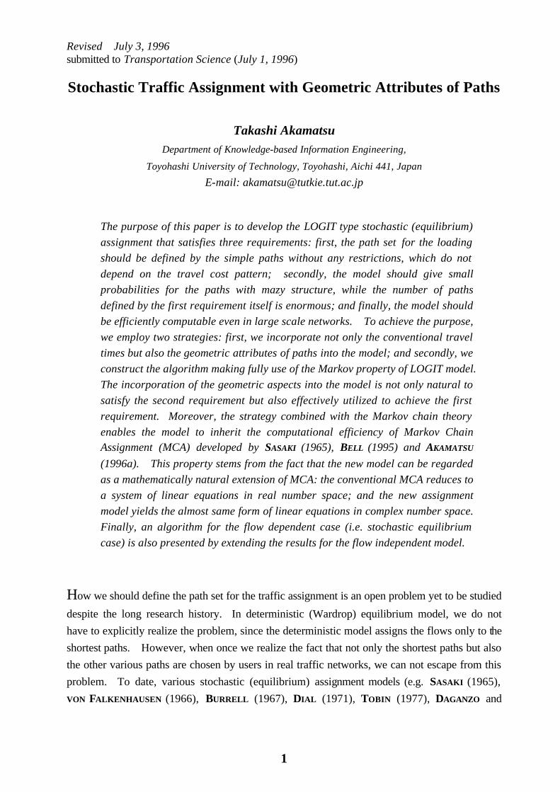
Revised July 3, 1996 submitted to Transportation Science (July 1, 1996) 1 Stochastic Traffic Assignment with Geometric Attributes of Paths Takashi Akamatsu Department of Knowledge-based Information Engineering, Toyohashi University of Technology, Toyohashi, Aichi 441, Japan E-mail: [email protected] The purpose of this paper is to develop the LOGIT type stochastic (equilibrium) assignment that satisfies three requirements: first, the path set for the loading should be defined by the simple paths without any restrictions, which do not depend on the travel cost pattern; secondly, the model should give small probabilities for the paths with mazy structure, while the number of paths defined by the first requirement itself is enormous; and finally, the model should be efficiently computable even in large scale networks. To achieve the purpose, we employ two strategies: first, we incorporate not only the conventional travel times but also the geometric attributes of paths into the model; and secondly, we construct the algorithm making fully use of the Markov property of LOGIT model. The incorporation of the geometric aspects into the model is not only natural to satisfy the second requirement but also effectively utilized to achieve the first requirement. Moreover, the strategy combined with the Markov chain theory enables the model to inherit the computational efficiency of Markov Chain Assignment (MCA) developed by SASAKI (1965), BELL (1995) and AKAMATSU (1996a). This property stems from the fact that the new model can be regarded as a mathematically natural extension of MCA: the conventional MCA reduces to a system of linear equations in real number space; and the new assignment model yields the almost same form of linear equations in complex number space. Finally, an algorithm for the flow dependent case (i.e. stochastic equilibrium case) is also presented by extending the results for the flow independent model. How we should define the path set for the traffic assignment is an open problem yet to be studied despite the long research history. In deterministic (Wardrop) equilibrium model, we do not have to explicitly realize the problem, since the deterministic model assigns the flows only to the shortest paths. However, when once we realize the fact that not only the shortest paths but also the other various paths are chosen by users in real traffic networks, we can not escape from this problem. To date, various stochastic (equilibrium) assignment models (e.g. SASAKI (1965), VON F ALKENHAUSEN (1966), BURRELL (1967), DIAL (1971), TOBIN (1977), DAGANZO and
Transcript of Stochastic Traffic Assignment with Geometric …akamatsu/Publications/PDF/...Chain Assignment that...
Revised July 3, 1996 submitted to Transportation Science (July 1, 1996)
1
Stochastic Traffic Assignment with Geometric Attributes of Paths
Takashi Akamatsu Department of Knowledge-based Information Engineering,
Toyohashi University of Technology, Toyohashi, Aichi 441, Japan
E-mail: [email protected]
The purpose of this paper is to develop the LOGIT type stochastic (equilibrium) assignment that satisfies three requirements: first, the path set for the loading should be defined by the simple paths without any restrictions, which do not depend on the travel cost pattern; secondly, the model should give small probabilities for the paths with mazy structure, while the number of paths defined by the first requirement itself is enormous; and finally, the model should be efficiently computable even in large scale networks. To achieve the purpose, we employ two strategies: first, we incorporate not only the conventional travel times but also the geometric attributes of paths into the model; and secondly, we construct the algorithm making fully use of the Markov property of LOGIT model. The incorporation of the geometric aspects into the model is not only natural to satisfy the second requirement but also effectively utilized to achieve the first requirement. Moreover, the strategy combined with the Markov chain theory enables the model to inherit the computational efficiency of Markov Chain Assignment (MCA) developed by SASAKI (1965), BELL (1995) and AKAMATSU
(1996a). This property stems from the fact that the new model can be regarded as a mathematically natural extension of MCA: the conventional MCA reduces to a system of linear equations in real number space; and the new assignment model yields the almost same form of linear equations in complex number space. Finally, an algorithm for the flow dependent case (i.e. stochastic equilibrium case) is also presented by extending the results for the flow independent model.
How we should define the path set for the traffic assignment is an open problem yet to be studied
despite the long research history. In deterministic (Wardrop) equilibrium model, we do not have to explicitly realize the problem, since the deterministic model assigns the flows only to the shortest paths. However, when once we realize the fact that not only the shortest paths but also the other various paths are chosen by users in real traffic networks, we can not escape from this problem. To date, various stochastic (equilibrium) assignment models (e.g. SASAKI (1965), VON FALKENHAUSEN (1966), BURRELL (1967), DIAL (1971), TOBIN (1977), DAGANZO and

2
SHEFFI (1977), FISK (1980), SHEFFI and DAGANZO (1980), DAGANZO (1982,1983), MIRCHANDANI and SOROUSH (1987), AKAMATSU (1989,1990, 1996a), BELL (1995), etc.) have tackled this problem. These models, either explicitly or implicitly, decide the set of paths for assigning flows by a priori criteria, and then the route-choice probabilities are calculated over the path set. Conventionally, some criteria for defining the path set have been employed. The simple and natural one is to define all the simple paths (i.e. the paths that do not traverse any links more than once), PS, as the path set for the assignment. To the author’s knowledge, however, no efficient algorithm for generating the flow pattern that completely satisfies this definition has been developed. This difficulty is mainly caused by the fact that the path enumeration is computationally impossible in real large-scale networks: the required storage and operations in enumerating simple paths increase exponentially with the growth of the network size. Note that the essential problem can not be theoretically overcome even if we utilize the conventional techniques such as column generation, simplicial decomposition, or Monte Carlo simulation. In order to avoid the path enumeration, some models / algorithms take the strategy that restricts the path set for the assignment to a certain subset of PS. For example, DIAL (1971) developed an efficient algorithm which generates the link flow pattern being consistent with the LOGIT type route choice model over the set of “efficient path”. Although the path restriction strategy is useful for the efficient calculation, it gives rise to the problem that the algorithm often generates unrealistic flow pattern (for the typical example, see AKAMATSU (1996a)). The restriction of paths also causes another troublesome problem in the flow dependent assignment: the path set for the loading varies with the change of the link cost pattern, and as a result, all the iterative algorithms in which the Dial’s algorithm is utilized can not be guaranteed to converge (for further detail, see AKAMATSU (1996b,1996c)). Recently, LAURENT (1996) proposed the modified definition of the efficient path, where the paths for the loading are restricted by some criteria based on the fixed “reference travel costs”. Although the definition has the advantage of stabilizing the paths in the flow dependent assignment, it suffers from over-restriction of paths: for example, in the ring-road network presented in Akamatsu(1996a), the definition can produce the unrealistic flow pattern as in the Dial’s algorithm. Recently, BELL (1995) and AKAMATSU (1996a) showed a definition being in a striking contrast to the restriction strategy: they analyzed the LOGIT assignment whose path set consists of all the possible paths, where even paths with cycles are permitted. The model overcomes the deficiency of the Dial’s algorithm, and is applicable to large scale networks, since it avoid path enumeration by applying the Markov chain theory (Henceforth, we call the model MCA: Markov Chain Assignment). The definition of the path set, however, is unnatural from the user’s behavior point of view, and therefore, it leaves rooms for various improvement. Thus, we can conclude that there is no assignment model equipped with both the behaviorally satisfactory path set and the computationally efficient algorithm.

3
This study aims to develop the efficient method for obtaining the flow pattern according to the LOGIT based stochastic (equilibrium) assignment model whose path set consists of only simple paths without any restrictions. To achieve the purpose, we employ two strategies: first, we incorporate not only the conventional travel times but also the spatial / geometric attributes of paths into the model; and secondly, we construct the algorithm exploiting the Markov property of the LOGIT model. The first strategy, obviously, can be justified from the user’s behavior view point. Our model due to this strategy assigns only a small amount of flow to the paths with excessively mazy structure even if the travel times of the paths are moderate. This is consistent with the observations in various traffic surveys. Interestingly, the incorporation of the geometric attributes not only improves the behavior model but also gives us the innovative method for constructing the set of simple paths. To be specific, we first define the geometric “rotation-angle” between adjacent links over the network, and then, by representing the rotations-angles along paths in complex number space, we obtain the method for distinguishing the cycles from the simple paths without explicit enumeration of paths. This method plays an important roll in developing the efficient assignment algorithm based on the second strategy. The second strategy implies that the assignment algorithm can avoid explicitly dealing with vast path variables. Namely, our algorithm operates only link variables instead of path variables, and it generates the link flows by origins / destinations. Note that this does not mean that our algorithm can produce less information than path based algorithms. From the Markov property of the LOGIT assignment, the link flows by origin / destination give us enough information to construct the corresponding path flows: we can obtain any path flows from the output of this algorithm “as wee needed”. To exploit this property, we construct the assignment algorithm based on the MCA developed by SASAKI(1965), BELL(1995) and AKAMATSU(1996a). Although the original MCA assigns the flows over the path set with cycles, the MCA combined with the first strategy can successfully eliminate all the cycles from the path set. Thus, we can achieve the purpose. The paper is organized as follows. We first briefly review the MCA that is consistent with LOGIT based route-choice model in Section 1, where we also draw attention to the problem caused by the cycle flows in MCA. With this problem in mind, the subsequent sections develop the methods for reducing / eliminating the cycle flows in MCA. In Section 2, we improve the MCA so as to avoid the simplest cycle flows of “U-turn”: we modify the MCA based on node-to-node transitions into the model based on link-to-link transitions. In Section 3 we then incorporate the geometric rotations of paths into the link-based MCA model. Based on these preliminary analyses, in Section 4 we consider the model whose path set is restricted to simple paths only, and then the novel method to eliminate the cycle flows without computational burden is developed. In Section 5, we discuss the extension to the flow dependent model. Finally, we present our conclusions and discuss the future research.

4
1.Preliminaries - LOGIT Assignment through Markov Chain Preliminary to the presentation of the new models, this section briefly reviews the Markov Chain Assignment that is consistent with LOGIT type route-choice model. For further detail, see AKAMATSU (1996a,b,c), BELL (1995) and SASAKI (1965).
1.1. Networks
Our model is defined on a traffic network G [N, L ] which has the set N of nodes, the set L of directed links and given set of origin-destination(OD) node pairs. The set N consists of three subset: the set of traversal nodes, N, that of origin nodes, O, and that of destination nodes, D. The number of nodes in each subset are n, g, and s, respectively. The link from node i to j is denoted as link (i, j). Each link in L has the travel cost, which is assumed to be fixed (i.e. flow independent). The extension to the flow dependent costs will be discussed in Section 5. In the followings, each node in G is assumed to belong to only one of the subsets N, O, or D: N O∩ = ∅ , N D∩ = ∅ , and O D∩ = ∅ . In addition, we assume that the number of links emanating from each origin is unique, and similarly, the number of links entering into each destination is unique. These assumptions are made only for the clarity of the presentation. In fact, they do not affect the generality of the subsequent models, since any traffic network can be modified so as to satisfies these assumptions without loss of generality (see Fig.1.1).
Origin, Destinationand Traversal Node
o d
Origin Destination
Fig. 1.1. (a) Original network. (b) Modified network.
1.2. Traffic Assignment through Markov Chain
We consider the network with multiple origins and single destination (“Many-to-One OD-pattern”). As can be seen in below, we can easily extend the model to the case of Many-to-Many OD-pattern by simply overlapping the flow pattern for each Many-to-One OD-pattern. The Markov Chain Assignment by SASAKI(1965) regards the nodes as the states in Markov chain, and the vehicles generated from origins are assumed to repeat the transition between the states according to the Markov chain rule. To formulate the model, let Q[d] be the transition probabilities matrix with the following structure:

5
1 g n
Q[d ] =0 0 00 0 Q1
Q2[d ] 0 Q[d ]
1 g n
(1.1)
where Q1 is a g×n matrix whose (o, i) component is 1 if the origin o is connected with the
traversal-node i, zero otherwise, Q2[d] is an n×1 vector whose i th component is 1 if the destination d is connected with
the traversal-node i, zero otherwise, Q[d] is an n×n matrix whose (i, j) component denotes the (non-zero) transition
probabilities, Qij, if traversal-node pair (i, j) is connected by a single link, zero otherwise.
Then, we easily see that the (i, j) component of Q[d]k is the sum of choice probabilities of k-
walks paths (i.e. the paths consisting of k nodes) between node pair (i,j). Therefore, the node-choice probabilities (conditional on being generated from each node) are given by the matrix series I + Q[dl + Q[dl
2 + Q[dl 3 + ···, and it converges to the following inverse matrix:
I + Q[d] + Q[d]2 + Q[d]
3 + ··· = [I-Q[d]]-1 = I 0 0P3[d ] I P1[d]
P2[d ] 0 P[d ]
, (1.2a)
P[d] = [I-Q[d]]-1, (1.2b)
P1[d] = Q1 P[d], P2[d] = P[d] Q2[d], P3[d] = Q1 P[d] Q2[d], (1.2c)
where P1[d] is a g×n matrix whose (o, i) component, P1[d] (i|o), denotes the probability that a
vehicle generated from origin o uses node i. Thus, we can obtain the link-choice probabilities by OD-pair, by substituting the P1[d](i|o) obtained in (1.2) into the following definitional formula:
pijod = P1[d](i|o)・Qij , (1.3)
where pijod denotes a probability that a vehicle with OD-pair (o,d) choose a link (i, j).
.
1.3. Transition Probabilities Consistent with LOGIT type Route Choice
At first sight, the MCA above has no background of behavior-theory, but it leads to the LOGIT based assignment: AKAMATSU (1996a) showed that MCA yields the flow pattern that is consistent with the LOGIT type route choice model, if the transition probabilities are given by
Qij =Q[d](j|i) = Wij Vjd / Vid or Q[d] =V2[d]-1 W V2[d], (1.4)
where Wij ≡ exp[−θ tij], (1.5)

6
V Cid rid
r R id≡ −
∈ ∞
∑
exp[ ]θ , (1.6)
tij : the cost of link (i, j), θ : the sensitivity parameter of LOGIT model,
Rid∞ : the set of all the possible paths between traversal-node i to destination d,
C trkd
ijij L
r ijkd≡
∈∑ δ , : the cost of r th path from node k to destination d,
V2[d] = an n×n diagonal matrix whose (i, i) diagonal component is Vid.
Note that we can deal with the Many-to-Many OD pattern by simply defining the transition probabilities for Many-to-One OD patterns by each origin.
How we calculate the Vid defined in (1.6) is not self-evident since the definition requires the summation with respect to infinite paths. Nevertheless, BELL (1995) showed that it can be obtained by the simple matrix operations as follows. Let W be the “impedance” matrix with the following form:
s g n
W =0 0 00 0 W1
W2 0 W
s g n
(1.7)
where W1 is a g×n matrix whose (o, i) component is 1 if the origin o is connected with the
traversal-node i, zero otherwise, W2 is an n×s matrix whose (i, d) component is 1 if the destination d is connected with
the traversal-node i, zero otherwise, W is an n×n matrix whose (i, j) component is Wij = exp[−θ tij] if traversal-node pair
(i, j) is connected by a link, zero otherwise.
Then, it follows that the (i, j) component of W k is the sum of exp[−θ Crij ] over the k-walks paths
between node pair (i, j). Therefore, the matrix V is given by I + W + W2 + W3 + ···, and it converges to the following inverse matrix:
I + W + W2 + W3 + ··· = [I-W]-1 = I 0 0
V3 I V1
V2 0 V
(1.8a)
V = [I-W]-1, V1 = W1 V, V2 = V W2, V3 = W1 V W2, (1.8b)
where the (o, i) component of matrix V1, the (j, d) component of matrix V2 , and the (o, d) component of matrix V3 are defined as V Coi r
oir
= −∑ exp[ ]θ ,V Cjd rjd
r= −∑ exp[ ]θ ,and
V Cod rod
r= −∑ exp[ ]θ , respectively.

7
1.4. LOGIT Assignment through Markov Chain
To sum up, we can obtain the link-choice probabilities that are consistent with LOGIT model by the following procedures:
Step 1: (a) Calculate the variable V by (1.8), (b) Determine the transition matrix Q by substituting the V into (1.4). Step 2: (a) Compute the node-choice probabilities by the Markov Chain formula (1.2), (b) Calculate the link-choice probabilities by (1.3). It is worth mentioning that the calculation in Step 2 reduces to the simple calculation as follows. Substituting (1.4) into (1.2), the node-choice probabilities yields
P1[d] = Q1 [I-Q[d]]-1 = Q1 [I-V2[d]-1 W V2[d]]-1
= Q1 V2[d]
-1 [I-W]-1 V2[d]
= Q1 V2[d]-1 V V2[d] . (1.9a)
That is, the (o,i) component of P1[d], P1[d](i|o) = P(i|o,d), is
P(i|o,d) = δ okk
∑ {(1 / Vkd) Vki Vid } = Voi Vid / Vod . (1.9b)
Therefore, the the flow on link (i, j) with OD-pair od, xijod, is given by the following formula
without explicit calculation of the inverse matrix [I-Q[d]]-1:
xijod =qod pij
od = qod P(i|o,d)・Q[d](j| i) = qod (Voi Vid / Vod )・(Wij Vjd / Vid)
= qod Voi Wij Vjd / Vod , (1.10)
where qod is the OD-flow between o and d.
1.5. The Problem Caused by Cycle Flows
The model above has a solution (i.e. the left hand side of (1.8a) converges and all the components take positive value) if and only if the spectral radius of W,ρ(W), is less than unity:
ρ(W)=Max.i
λ i < 1, (1.11)
where λi is the i th eigenvalue of matrix W. The condition (1.11), however, may not be
satisfied in some cases. For example, when the network has many cycles with zero costs, the network can induce infinite cycle flows, which means the non-existence of the solution. There also may be possibilities that unrealistic cycle flows are assigned even if the model has a solution. With this problem in mind, we will develop methods for reducing / eliminating the cyclic flows in the subsequent sections.

8
2.Markov Chain Assignment based on Link-to-Link Transitions
2.1. Markov Chain Assignment on a Line-Graph
The cycle flows that have the worst effect on the assignment flow pattern in practical applications are “U-turn” flows in a pair of opposite-directional links that connect the same node-pair. For example, the network shown in Fig.2.1 can induce excessive U-turn flows that repeat going between links 4 and 6. This kind of cycle flows, however, can be easily eliminated by using the concept of “line-graph” (for the definition, see, for example, WILSON(1985), TAKENAKA(1989) etc.).
1
2
3
4o d1
2
3
4
5
6
7
8
Fig. 2.1. An example network.
Let us consider a line-graph G*(N*, L*) of a given original network G(N, L): each node in N* has one-to-one correspondence to a link in L, and the nodes in N* are connected by links in L* if the corresponding links in L are adjoining. Note here that the “U-turn” movement in G(N, L) corresponds to a movement between a pair of nodes in N*. Therefore, we construct L* eliminating the links that connect such node pairs in N*. Then any assignment models on the graph G*(N*, L*), clearly, can not generate the “U-turn” flows. Thus, by considering a Markov chain assignment on G*(N*, L*), we can obtain a link flow pattern explicitly avoiding the “U-turn” flows. Fig.2.2 illustrates the line-graph G*(N*, L*) for the example network G(N, L) shown in Fig.2.1. In the line-graph the nodes 4 and 6 are not mutually connected, and therefore, we see that the Markov chain assignment on G*(N*, L*) does not generate any cycle flows.
1
2
3
4
6
7
8
5
Fig. 2.2. A line-graph.
It is worth a mention in passing that this technique can be used not only for eliminating the cycles but also for representing turn-restrictions due to traffic control policies: we have only to eliminate the appropriate links in the line-graph corresponding to the turn-restrictions.
9
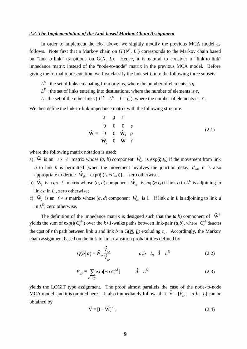
2.2. The Implementation of the Link based Markov Chain Assignment
In order to implement the idea above, we slightly modify the previous MCA model as follows. Note first that a Markov chain on G*(N*, L*) corresponds to the Markov chain based on “link-to-link” transitions on G(N, L). Hence, it is natural to consider a “link-to-link” impedance matrix instead of the “node-to-node” matrix in the previous MCA model. Before giving the formal representation, we first classify the link set L into the following three subsets:
LO : the set of links emanating from origins, where the number of elements is g,
LD : the set of links entering into destinations, where the number of elements is s, L : the set of the other links ( LO ∪ LD ∪ L =L ), where the number of elements is l .
We then define the link-to-link impedance matrix with the following structure:
s g
sg
l
l
$ $$ $
W WW W
=
0 0 00 0
01
2
(2.1)
where the following matrix notation is used: a) $W is an l× l matrix whose (a, b) component $Wab is exp(?θ tb) if the movement from link
a to link b is permitted [when the movement involves the junction delay, dab, it is also appropriate to define $Wab = exp(?θ (tb +dab))], zero otherwise;
b) $W1 is a g× l matrix whose (o, a) component $Woa is exp(?θ ta) if link o in LO is adjoining to
link a in L , zero otherwise; c) $W2 is an l×s matrix whose (a, d) component $Wad is 1 if link a in L is adjoining to link d
in LD, zero otherwise.
The definition of the impedance matrix is designed such that the (a,b) component of $Wk yields the sum of exp(?θ Cr
ab ) over the k+1-walks paths between link-pair (a,b), where Crab denotes
the cost of r th path between link a and link b in G(N, L) excluding ta. Accordingly, the Markov chain assignment based on the link-to-link transition probabilities defined by
Q b a WV
Vabbd
ad
( ) $$
$$
$
= ∀ ∈a b, L, $d ∈LD (2.2)
$ exp[ ]$$
$
V Cad r
ad
r Rad
≡ −∈ ∞
∑ θ $d ∈LD (2.3)
yields the LOGIT type assignment. The proof almost parallels the case of the node-to-node MCA model, and it is omitted here. It also immediately follows that ˆ V = [ ˆ V ab ; ∀ ∈a b, L] can be
obtained by ˆ V = [I − ˆ W ]−1 , (2.4)

10
and that $V1 ≡ [ $$Voa ;∀ ∈ ∀ ∈a L o, $ LO], $V2 ≡ [ ˆ V
a ˆ d ;∀ ∈ ∀ ∈a L d, $ LD], and $V3 ≡ [ $
$ $Vod
;∀ ∈$o LO,
∀ ∈$d LD ] are, respectively, given by
$ $ $V W V1 1= , $ $ $V V W2 2= and $ $ $ $V W V W3 1 2= . (2.5)
Finally, the formula for the link flow can be obtained by utilizing the fact that the link-choice probability means the node-choice probability in the line-graph. That is, considering the correspondence to (1.9b) in the node-to-node MCA model, we have the following formula for the flow on link a with OD pair od:
x q V V Vaod
od oa ad od= $ $ / $
$ $ $ $ , $o ∈LO, $d ∈LD. (2.6)
Thus, we can efficiently obtain the link flow pattern that is consistent with LOGIT model explicitly avoiding the “U-turn” flow. It is expected in many practical applications that the modified MCA model can avoid the problem that the solution does not exist due to the excessive cycle flows. Nevertheless, the model may not necessarily yields the satisfactory flow pattern, since there still be a possibility that excessive flows are assigned on various possible cycles except “U-turn”. In the next section we will further devise another method for mitigating the cycle flows.
3. Markov Chain Assignment with Geometric Rotations
3.1. Rotation-angles between Links
Conventional stochastic assignment models assign the flows to many paths by some criteria based on the one-dimensional factor “travel time”. In contrast, various traffic surveys have reported that the share of “mazy” paths with many zigzaggings or turns are very small even if the travel times are moderate. In light of this fact, it is reasonable to introduce not only the travel time but also the geometric factors into the path-choice model. To develop such a model, consider first the 2-dimentional Euclid geometric space to represent the geographic position of nodes in a traffic network. Then the links can be represented as vectors on 2-dimentional real number space R2. In other word, we can regard a traffic network as a set of vectors on R2. Using the vectors, we define the rotation-angle between mutually adjacent links a and b as follows:
ωab =
sgn(r a ,
r b )⋅ cos −1
r a ⋅
r b
r a r b
, 0 ≤ω ab ≤ π , (3.1)
where r a is a vector representing link a on R2; and sgn(
r a ,
r b ) = +1 if the movement from
r a to

11
r b is right-handed turn, -1 otherwise (See Fig.3.1).
ra
rbωab
+−
ωac
rc
Fig. 3.1. The rotation-angle between mutually adjacent links
Then the total rotation-angle along r th path between OD pair od is naturally introduced as the sum of the absolute angles between adjoining links on the path:
Drod
ab r abod
a b
≡∈
∑
ω δ ,( , ) Λ
, (3.2a)
where δr abod, is 1 if the mutually adjacent links a and b are on r th path between OD pair od, zero
otherwise, Λ is the set of link-pairs where the two links are mutually adjacent. Similarly, the “net” total rotation-angle for the path is also defined as follows:
Erod
ab r abod
a b
≡∈
∑
ω δ ,( , ) Λ
. (3.2b)
In addition, we define the rotation-angle between links that are not mutually adjacent. While the definition is basically the same as that for the mutually adjacent links, we should note the definition when two links are in a parallel position. The angle between the parallel links a and b is defined as follows:
Step 1: add two virtual links between the links a and b so as to construct a cycle (See Fig.3.2);
Step 2: if the cycle is right-handed then ωab = π and ωba = −π, otherwise ωab = −π and ωba = π.
ra
rb
ra
rb
Fig.3.2. (a) Right-handed link-pair. (b) Left-handed link-pair.
12
3.2. LOGIT assignment with Geometric Rotations
To incorporate the geometric factors into the path-choice model, suppose that the systematic utility for the r th path between o and d, Ur
od, is represented as
Urod = −θ Cr
od − σ Drod , (3.3)
whereσis a “sensitivity” parameter for the total rotation-angle. Then, by assuming the error
term of the utility function to be i.i.d Gumbel distribution, the probability that users choose r th path between OD pair od yields
PC D
C Drod r
odrod
rod
rod
r Rod
=− −
− −∈ ∞
∑exp[ ]
exp[ ]θ σ
θ σ
=
∈ ∞
∑
A
Arod
rod
r Rod
, (3.4a)
A C Drod
rod
rod≡ − −exp[ ]θ σ , (3.4b)
and the resulting link flow pattern is given by
x q Paod
od rod
r aod
r Rod
=∈ ∞
∑ δ , . (3.5)
Since this model is basically a LOGIT model, we can construct the corresponding MCA. Unlike the previous MCA, we can expect that this MCA does not give rise to much cycle flows, since the paths with cycles have large negative utilities due to the rotation-angles. The algorithm for this model is almost same with that for the previous MCA model. The only difference is the slight modification of the link impedance matrix: the (a,b) component of the matrix is defined as
$ exp[ ]W tab b ab= − −θ σ ω . (3.6)
The reason why this modification yields the LOGIT assignment model in (3.4a), (3.4b) and (3.5) can be easily understood from the fact that the (a,b) component of $Wk yields the sum of exp( − −θ σ C Dr
odrod ) over the k+1-walks paths between link-pair (a,b).
Thus, one may expect that the model combined with the technique in Section 2 greatly reduces cycle flows in many cases. The model, however, does not achieve our purpose, since it still remains a possibility of generating unrealistic flow patterns. For example, the model can not distinguish between a path with one cycle and a simple path with 4 rectangular turns, while almost all real users think the former path unreasonable. Recall here that the model shown above did not utilize the net total rotation-angles Er
od defined in (3.2b) at all. Interestingly, the exploitation of the Er
od gives us the innovative method to achieve the complete elimination of cycle flows, which will be presented in the next section.

13
4.Complete Elimination of Cycle Flows
4.1. LOGIT type Route Choice Model without Cycles
In this section we will consider the method for obtaining the link flow pattern according to the following LOGIT model:
PC D
C Drod r
odrod
rod
rod
r Rod
=− −
− −∈∑
exp[ ]
exp[ ]( )
θ σθ σ
0
=
∈∑
A
Arod
rod
r Rod ( )0
, (4.1a)
x q Paod
od rod
r aod
r Rod
=∈∑ δ ,
( )0
, (4.1b)
where the Rod(0) is the set of simple paths between nodes o and d. Note that the path set in (4.1), unlike the MCA model in Section 3, consists of the simple paths only; the cycle flows are explicitly eliminated. The main focus here is, thus, to develop the method for achieving the complete elimination of cycle flows by exploiting the Er
ab introduced in the previous section. Just as in the case of the previous MCA, the method presented in this section consists of the following two steps: Step 1: Calculate the matrix $V whose (a,b) component is defined as
$( )
V Aab rab
r Rab≡
∈∑
0. (4.2)
Step 2: Compute the link flows by
x q X Vaod
od aod
od= / $ , (4.3a)
X Aaod
rod
r aod
r Rod
≡∈∑ δ ,
( )0
. (4.3b)
Before going into the detailed discussions on the steps above, we will first examine the basic properties of the net rotation-angle Er
ab in 4.2. Making use of the properties, we then develop a novel method for achieving Step 1. The considerations on the method is divided into two parts, which are presented in the subsequent sections 4.3 and 4.4, respectively. Finally, the method for calculating the Xa
od in Step 2 is presented in 4.5. 4.2. Basic Properties of the Path Rotation-angle
Let us consider the properties of the net rotation-angle defined in (3.2). First, it is easily observed that the rotation-angle of a path between links a and b, Er
ab, is equal to −wba if the path contains no cycles. For example, the path (a,b,c) in Fig.4.1 (a) contains no cycles, and the rotation-angle is Eac = ωab + ωbc = −ωca or Eac + ωca = 0. Next, consider the cases where the path contains cycles. In the example of Fig.4.1 (b), the path (a,b,c,d,e) contains one left-handed

14
cycle, and the rotation-angle is Eae + ωea = ωab + ωbc + ωcd + ωde+ ωea = −2π. Similarly, the path (a,b,c,d,b,c,d,e) has double left-handed cycles, and Eae + ωea = −4π. Thus, we see that Er
ab + wba =2mπ (m=±1,±2,...) for the paths with cycles, and that the value of Er
ab + wba can be a
“detector” that shows whether the path contains cycles or not. Note, however, that there is a particular case that the Er
ab + wba can be zero even if the path contains cycles: when we consider the path where the number of right-handed cycles, NR , is equal to that of left-handed cycles, NL , the Er
ab + wba yields zero since the rotation-angles for the respective cycles mutually cancel.
ra
rc
rc
rb
ωab
ωbc
ωca
ra
rb
rc
rd
re
re
ωea
ωbc
ωcd
Fig. 4.1. (a) Path (a,b,c) (b) Path (a,b,c,d,e)
To give the formal representation of these properties, we denote by Rkab the set of k-walks
paths between links a and b (paths from link a to link b consisting of k links). The path set can be classified into the following three subsets:
Rkab ( )0 : the subset of Rk
ab , which consists of the only paths containing no cycles,
Rkab ( )1 : the subset of Rk
ab , which consists of the paths such that NR ≠ NL,
Rkab ( )2 : the subset of Rk
ab , which consists of the paths such that NR =NL ≠ 0.
Similarly, we also classify the set of paths between links a and b, Rab, into three subsets:
Rab(m) ≡ ∪=
∞
kRk
ab m1
( ) for m=0,1, and 2.
Then, the path rotation-angle satisfies the following:
E
r R
m m r R
r Rrab
ba
ab
ab
ab
+ =
∈
= ± ± ∈
∈
ω π
0
0
( )
( , ,... ) ( )
( )
0
2 1 2 1
2
( . )
( . )( . )
4 4
4 44 4
a
bc
In the subsequent secction 4.3, we first consider the method for calculating the sum of Arab
for the path set Rab(0)∪Rab(2) (i.e. we eliminate the sum for Rab(1)); and then we proceed to the method to further exclude the path set Rab(2) as well as Rab(1) in section 4.4.

15
4.3. Elimination of the Path Set R(1)
Suppose for the moment that the path set Rod(2) is excluded from Rod by an appropriate method: we assume that Rod = Rod(0) ∪ Rod(1). Then, the $Vod defined in (4.2) can be
re-written as follows:
$( )
V Aod rod
r Rod=
∈∑
0 = δ ω( )E Ar
oddo r
od
r Rod+ ⋅
∈∑ , (4.5a)
where δπ
( ). .
z if z 0
otherwise i e z = 2m m= 1, 2,...≡
=± ±
10
( , )
. (4.5b)
Recall here the Fourier series expansion of Dirac’s delta-function:
δπ
( ) coszT T
nT
zn
= +
=
∞
∑1 2 2
1
=
=−∞
∞
∑1 2T
inT
zn
exp π
for − ≤ ≤T z T/ /2 2 , (4.6)
where i denotes an imaginary unit. From (4.5) and (4.6), we see that $Vod is represented by the
(complex) exponential function, which can be decomposed into link variables. Thus, if we construct the MCA model based on the appropriate impedance matrix that is consistent with (4.6), the sum of Ar
ab for Rab(1) would naturally be eliminated. The procedure presented below is, in essence, the realization of this idea. Let ˆ W (n, N) be the “complex impedance” matrix with the following (a, b) component:
$ exp[ ]( , )W t inNab b ab abn N = − − +θ σ ω ω = Wab Yab(n,N) (4.7)
where W tab b ab≡ − −exp[ ]θ σ ω ,Y inNab abn N( , ) exp[ ]≡ ω , and (n,N) are the integers satisfying
1 ≤ n ≤ N . Then, the (a, b) component of the k th power of the matrix, ˆ W ab (n,N )k , yields
$ exp[ ]( , )W A i EnNab r
ab
kab
rabn N k
r R=
∈ +
∑ 1
, (4.8)
where Rk +1ab is the set of k+1-walks paths between links a and b. Therefore, it immediately
follows from (4.4a) and (4.4c) that
$ exp[ ( ) ]
exp[ ( ) ]
( , ) ( , )
( ) ( ) ( )
W Y A i EnN
A A A i EnN
ab ba rab
kab
rab
ba
rab
kab
rab
kab
rab
kab
rab
ba
n N k n Nr R
r R r R r R
= +
= + + +
∈ +
∈ + ∈ + ∈ +
∑
∑ ∑ ∑1
1 1 10 2 1
ω
ω . (4.9)

16
The present subject here is to eliminate the third term of the r.h.s. of (4.9), which leads us to exclude the summation with respect to the path set Rab(1) in the calculation of $V . In order to construct the elimination method, recall the fact that the value of Er
ab + ω ba in the third term must be 2mπ , (m =±1,2,...). Considering this property and the (4.6), we have
1
11
11NA i E
nN
Arab
kab
rab
ban
N
rab
kabr R r R N
∈ +
= ∈ +
∑∑ ∑+ =( ) ( )
exp[ ( ) ]ω , (4.10)
where Rk +1ab (N) is the subset of Rk +1
ab (1) such that Erab + ω ba = (2Nπ )× l , ( l =±1,±2,...).
Table 4.1 shows the simple numerical example for (4.10) when there is only a single route, N = 3, and Ar
ab=1. The number in each cell denotes the value of
Re(exp[ i znN
]) = COS ( znN
) = COS (2 mπnN
),
where zαErab + ω ba, and the rows and the columns correspond to n = 1,2,3 and m = 1,2,...,
respectively. The final row denotes the Σn COS (z n/N)) for z = 2mπ (m =0,1,2,...). As seen in the table, the Σn COS (z n/N)) yields zero, except the cases where z = (2Nπ )× l = 0, 6π, 12π,.... Thus, the r.h.s. of the (4.10) reduces to the sum over the paths such that Er
ab + ω ba = (2Nπ )× l .
Table 4.1. The numerical example of (4.10): COS (z n/N) and Σn COS (z n/N) for zαEr
ab + ω ba =2 mπ (m =0,1,2,...).
n ↓
m → zαEr
ab + ω ba → 0 0
1 2π
2 4π
3 6π
4 8π
5 10π
6 12π
...
1 COS ( z / 3) → 1.0 -0.5 -0.5 1.0 -0.5 -0.5 1.0 ... 2 COS (2z / 3) → 1.0 -0.5 -0.5 1.0 -0.5 -0.5 1.0 ... 3 COS (3z / 3) → 1.0 1.0 1.0 1.0 1.0 1.0 1.0 ...
Sum. 3.0 0.000 0.000 3.0 0.000 0.000 3.0 ...
Note that the period (of z) that Σn COS (z n/N)) takes non-zero value grows as we increase N. Hence, by letting N be infinity in (4.10), we can eliminate the summation for the Rk +1
ab (1):
limN→∞
1N
Arab
r∈R k+1 ab (1)
∑ exp[i (E rab + ωba )
nN
]n=1
N
∑
= 0 . (4.11)
Combining (4.9) and (4.11), we have
limN→∞
1N
Wab(n,N)k Yba (n, N)n=1
N
∑
= Ar
ab
r∈ R k +1 ab (0)
∑ + Arab
r∈ R k+1 ab (2)
∑ , (4.12)
and furthermore, summing up (4.12) for k=1,2,..., gives us
17
lim ( , ) ( , )( ) ( )N
k
r R r RN
W n N Y n N A Aab ba
n
N
k
rab
abrab
ab→∞ ∈ ∈==
∞
∑∑ ∑ ∑
= +
1
11 0 2
.
Namely, the sum of Arab for the path set Rab(0)∪Rab(2) (i.e. the path set where the Rab(1) is
excluded) is given by the (a, b) component of the following matrix:
limN N→∞
1 ( )I Y∗ ∗ ∗+ + +=
∑ ( , ) ( , ) ( , ) ( , ) ( , )$ $n N n N n N n N n NT T T
n
N
W Y W Y 2
1
L
= limN N→∞
1 ( )[I W ] Y− − ∗=
∑ $ ( , ) ( , )n N n N T
n
N1
1
, (4.13)
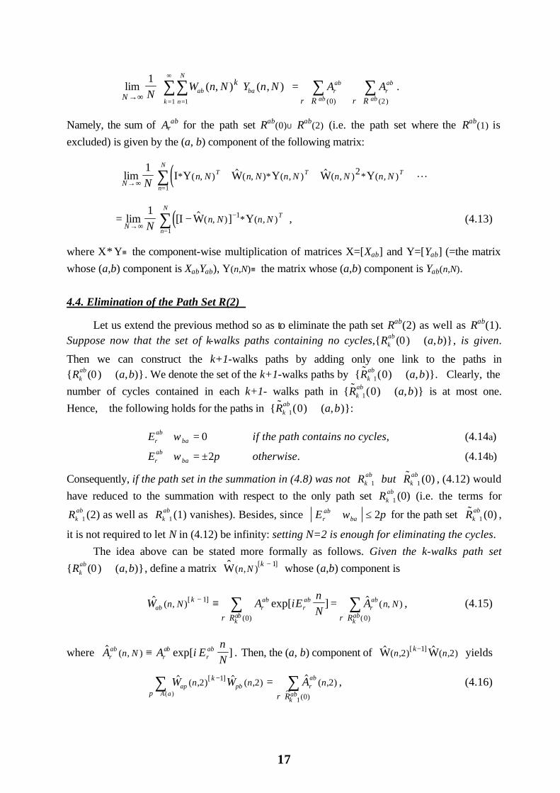
where X∗ Y≡the component-wise multiplication of matrices X=[Xab] and Y=[Yab] (=the matrix whose (a,b) component is XabYab), Y(n,N)≡the matrix whose (a,b) component is Yab(n,N). 4.4. Elimination of the Path Set R(2)
Let us extend the previous method so as to eliminate the path set Rab(2) as well as Rab(1). Suppose now that the set of k-walks paths containing no cycles,{Rk
ab (0) ∀(a,b)}, is given.
Then we can construct the k+1-walks paths by adding only one link to the paths in {Rk
ab (0) ∀(a,b)}. We denote the set of the k+1-walks paths by { ˜ R k+1ab (0) ∀(a,b)}. Clearly, the
number of cycles contained in each k+1- walks path in { ˜ R k+1ab (0) ∀(a,b)} is at most one.
Hence, the following holds for the paths in { ˜ R k+1ab (0) ∀(a,b)}:
Erab +ωba = 0 if the path contains no cycles, (4.14a)
Erab +ωba = ±2π otherwise. (4.14b)
Consequently, if the path set in the summation in (4.8) was not Rk +1ab but ˜ R k +1
ab (0) , (4.12) would have reduced to the summation with respect to the only path set Rk +1
ab (0) (i.e. the terms for
Rk +1ab (2) as well as Rk +1
ab (1) vanishes). Besides, since Erab
ba+ ≤ω π2 for the path set ˜ R k +1ab (0) ,
it is not required to let N in (4.12) be infinity: setting N=2 is enough for eliminating the cycles. The idea above can be stated more formally as follows. Given the k-walks path set {Rk
ab (0) ∀(a,b)}, define a matrix ˆ W (n,N )[k − 1] whose (a,b) component is
$ exp[ ] $( , ) ( , )[ ]
( ) ( )
W A iEnN
Aab rab
rab
kab
rab
kab
n N n Nk
r R r R
− ≡ =∈ ∈
∑ ∑1
0 0
, (4.15)
where $ exp[ ]( , )A A i EnNr
abrab
rabn N ≡ . Then, the (a, b) component of $ $( ,2) ( ,2)[ ]W Wn nk−1 yields
$ $( ,2) ( ,2)[ ]
( )
W Wap pbA a
n nk
p
−
∈∑ =1 $ ( , )
~( )
Arab
kab
nr R
2
1 0∈ +
∑ , (4.16)
18
where A(a) denotes the set of links emanating from the end-node of link a (Note that the $ $( ,2) ( ,2)[ ]W Wn nk−1 is not equal to the $ ( ,2)W n k nor the $ ( ,2)[ ]W n k while it plays a similar roll
with the $ ( ,2)W n k in (4.12)). Applying the same argument as (4.12) to (4.16), we see that the sum of Ar
ab for the path set Rk +1ab (0) is given by the (a,b) component of the following matrix:
( )~ $ $[ ] [ ]( ,2) ( ,2) ( ,2)W W W Yk k
nn n n T≡ ∗−
=∑1
21
1
2
. (4.17)
Since the $Vab in (4.2) is defined as the sum of Arab for the path set Rab(0) = ∪
=
∞
kkabR
1(0), the matrix
$V with the component $Vab can be obtained by simply summing up (4.17) with respect to k. In
addition, considering the fact that the number of links contained in the path without no cycles is at most l (=the number of links in L), we have
$ ~ ~ ~ ~[ ] [ ] [ ] [ ]V I W W W W= + + + + =−
=
−
∑1 2 1
0
1
L ll
k
k, (4.18)
where ˜ W [0] ≡ I (a unit matrix). We showed thus far the method for obtaining $V when the path set {Rk
ab (0) ∀(a,b)} or
the matrix $ ( ,2)[ ]W n k − 1 are given in calculating ~( ,2)[ ]W n k . In the following, we consider the
method for obtaining the matrix $ ( ,2)[ ]W n k − 1 such that it works successively in ascending
order of k : first, we set $ : $( ,2)[ ] ( ,2)W W n n1 = for k=1; and then, for each k≧2, we calculate
the matrix $ ( ,2)[ ]W n k using the $ ( ,2)[ ]W n k − 1 previously obtained. Thus, the present subject is
to constitute the appropriate formula for the successive calculation for k≧2. To find the formula, let us first compare the definition of $ ( ,2)[ ]W n k and the $ $( ,2) ( ,2)[ ]W Wn nk−1 : the (a,b) component of $ $( ,2) ( ,2)[ ]W Wn nk−1 is given by (4.16), and that of $ ( ,2)[ ]W n k is defined as
$ $( ,2) ( ,2)[ ]
( )
W Aab rab
kab
n nk
r R
≡∈ +
∑1 0
. (4.15’)
Note here that the set ~Rkab+1 (0) in (4.16) can be classified into two subsets Rk
ab+1 (0) and ~Rk
ab+1 (1):
~Rkab+1 (0) =
~Rkab+1 (1) ∪ Rk
ab+1 (0) and ~Rk
ab+1 (1) ∩ Rk
ab+1 (0) = ∅ ,
where the path set ~Rkab+1 (1) is defined as ~Rk
ab+1 (0) ∩ Rk
ab+1 (1) (see Fig.4.2). Thus it follows that
$ $( ,2) ( ,2)[ ]
( )
W Wap pbA a
n nk
p
−
∈∑ −1 $ $ $( , ) ( , ) ( , )[ ]
( ) ( )~
W A Aab rab
kab
rab
kab
n n nk
r R r R
2 2 2
1 10 0
= −∈ + ∈ +
∑ ∑
=∈ +
∑ $ ( , )~
( )
Arab
kab
nr R
2
1 1
(4.19)

19
R k+1
ab
R k+1ab (1)
R̃ k+1ab (1)
R̃ k+1ab (0)
R k+1ab (0)
R k+1ab (2)
Fig. 4.2. The classification of k+1-walks paths.
Therefore, given a matrix Z(n,2)[k]
whose (a,b) component is defined as
Zab(n,2)[k] ≡
∈ +
∑ $~
( )
( ,2)Arab
kabr R
n
1 1
, (4.20)
we have the following successive equation for calculating $ ( ,2)[ ]W n k in ascending order of k:
$ : $ $( ,2) ( ,2) ( ,2) ( ,2)[ ] [ ] [ ]W W W Z n n n nk k k= −−1 . (4.21)
The Zab(n,2)[k]
can be calculated without explicitly dealing with path variables, while the definition in (4.20) is represented by the summation with respect to the path set ~Rk
ab+1 (1). Recall
now the particular property for ~Rkab+1 (1): if the k+1-walks path a → ・・・ → p → b belongs to ~Rk
ab+1 (1),
ˆ W ap(n,2)[ k−1] ˆ W pb (n,2) Yba (n,2)n=1
2
∑ = 0 . (4.22)
For the concrete example, consider two 5-walks paths between links a and b as shown in Fig.4.3. The path a → ・・・ → p → b belongs to ~R ab
5 (1) , where we can examine that (4.22) holds. On the other hand, for another path (a → ・・・ → q → b) that belong to R ab
5 (0), it is easily seen that (4.22) does
not hold.
p
q
a
b
Fig. 4.3. Example network to consider (4.22).

20
From this property, the Zab(n,2)[k]
is, clearly, computed by
Zab(n,2)[k]
:=
$ $( ,2) ( ,2)[ ]W Wap pbn nk
p ab
−
∈
∑ 1
Ψ
, (4.23)
where Ψab is the set of links {p} such that (4.22) hold. Thus, the $ ( ,2)[ ]W n k can be
successively obtained in ascending order of k by the formula (4.21)-(4.23).
4.5. Calculation of Link Flows
We are now in a position to discuss the method for obtaining the link flows. For the calculation we can not use the formula for the MCA model presented in Section 2:
x q V V Vaod
od oa ad od= $ $ / $ , o ∈LO, d ∈LD. (2.6)
The reason is that the denominator of (2.6) contains the term for the paths with cycles. More specifically, the multiplication of $Voa and $Vad yields
$ $( ) ( )
V V A A Aoa ad roa
rad
rod
r R r R r Roa adaod
=
=
∈ ∈ ∈∑ ∑ ∑
0 0
, (4.24)
where Raod is the set of paths in which each path is constructed by connecting the following two
kinds of paths: the paths between links o and a in Roa(0), and the paths between links a and d in Rad(0). Note that the path (o→ ・・・ → a→ ・・・ → d) in Ra
od can contain cycles, even if both the
paths (o→ ・・・ → a) and (a→ ・・・ → d) contain no cycles (for the simple example, see Fig. 4.4). Therefore, we must replace the $ $V Voa ad in (2.6) with the variable Xa
od defined as
X A Aaod
rod
r aod
r Rrod
r Rodaod
≡ =∈ ∈∑ ∑δ ,
( ) ( )0 0
, (4.25)
where Raod (0) denotes the subset of Ra
od whose elements are restricted to the simple paths.
a
od
Fig. 4.4. The path (o→ ・・・ → a→ ・・・ → d) containing a cycle. To consider the method for calculating the Xa
od, we first classify the set Raod (0) by the
number of links contained in the paths; we denote by Raod (0: j+k ) the set of the simple paths
between o and d where each path is constructed by connecting the following two kinds of paths:

21
the j-walks paths between o and a, and the k-walks paths between a and d. Corresponding to this classification, we define X a
od j k [ ]+ as the sum of Arod for the paths in Ra
od (0: j+k ):
X Aaod j k
rod
r R j kaod
[ ]
( : )
+
∈ +
≡ ∑0
. (4.26)
Clearly,
X Xaod
aod j k
k
j
j
= +
=
−
=∑∑ [ ]
11
ll
. (4.27)
In precisely the same fashion, we also classify the path set Raod , and we denote by Ra
od (j+k) the subset corresponding to the subset Ra
od (0: j+k ) for the set Raod (0).
The key to calculate the X aod j k [ ]+ is the fact that the number of cycles contained in any
paths in Raod (j+k ) is at most one. From this fact, we see that the sum of Ar
od for the paths in Ra
od (0: j+k ), X aod j k [ ]+ , can be obtained by subtracting the terms such that Er
ab +ωba = ±2π from the sum for the paths in Ra
od (j+k ). Hence, by applying the similar method as shown in 4.4,
we obtain
( )X W W Yaod j k
oaj
adk
don
n n n [ ] [ ] [ ]$ $( ,2) ( ,2) ( ,2)+
=
= ∑12 1
2
. (4.28)
Substituting this into (4.27), we have
X aod ( )=
==
−
=∑∑∑1
2 1
2
11
$ $( ,2) ( ,2) ( ,2)[ ] [ ]W W Yoaj
adk
donk
j
j
n n nll
====
∑∑∑12 111
2
Y W Wdo oaj
adk
kjn
n n n( ,2) ( ,2) ( ,2)$ $[ ] [ ]ll
==
∑12 1
2
Y V Vdo oa adn
n n n( ,2) ( ,2) ( ,2)~ ~
,
(4.29)
where
~ $( ,2) ( ,2)[ ]V Wab abk
k
n n≡=
∑1
l
. (4.30)
As shown in Section 4.4, the $ ( ,2)[ ]Wabkn can be computed in ascending order of k, and
therefore, the ~( ,2)Vab n in (4.29) also can be easily obtained. Thus, we see that the link flows
can be calculated by the following formula:
x q V V Y Vaod
od oa adn
do odn n n==
∑12 1
2
~ ~ / $( ,2) ( ,2) ( ,2) , o ∈LO, d ∈LD. (4.31)

22
5.Extension to the Stochastic Equilibrium Model
In this section we first discuss the implementation issues of the model presented in the previous section, and then we extend the model and algorithm to the flow dependent case. 5.1. The Outline of the Assignment Algorithm
The considerations for the assignment over a path set R(0) so far can be summarized as the following algorithm:
Step 0: Initialization
for each (a,b) in L × L do begin $ :Vab = 0 ;
~ :[ ]Wab1 0 = ;
for n = 1 to 2 do begin
Yab(n) := exp[i ωab / n]; $ : exp[ ]( )[ ]W tab b abn 1 = − −θ σ ω Yab(n) ; (5.1)
end end;
Step 1: Calculation of Matrix [ $Vab ]
for k = 2 to l do begin for each (a,b) in L × L do begin
$ ( )[ ]Wabk1 := 0; $ ( ) [ ]Wab
k2 := 0; ~[ ]Wab
k := 0;
for each p in A(a) do begin X := 0; for n = 1 to 2 do begin
wp(n) := $ ( )[ ]Wapkn −1 $ ( ) [ ]Wpb n 1 ; X := X + wp(n) Yba(n) (5.2)
end;
for n = 1 to 2 do if X ≠ 0 then $ ( )[ ]Wabkn := $ ( )[ ]Wab
kn + wp(n) (5.3)
end; for each q in A(a) do for n = 1 to 2 do
~[ ]Wabk :=
~[ ]Wabk + wq(n)Ybq(n) ; (5.4)
$Vab := $Vab + ~[ ]Wab
k / 2; (5.5)
for n = 1 to 2 do ~Vab (n) :=
~Vab (n) + $ ( )[ ]Wabkn (5.6)
end end;
Step 2: Calculation of Link Flows by OD-pairs
for each (o,d) in LO × LD do
for each a in L do xaod :=
12 1
2
q V n V n Y n Vod oa ad do odn
~ ( ) ~ ( ) ( ) $=
∑ ; (5.7)
23
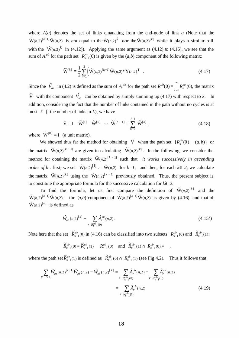
5.2. Some Improvement of the Algorithm
In 5.1, we showed only a prototype of the algorithm. For the practical applications, however, the algorithm should be improved from the view point of both the required storage and the computational effort. First, we do not have to store $ ( )[ ]W n ab
k or ~[ ]Wabk for all k : obviously,
only the temporal ~[ ]Wabk should be stored. Secondly, it is expected in many cases that we can
truncate the algorithm before k reaches l , since the maximum number of links contained in any simple paths in practical networks is usually much smaller than l . Finally, it is not necessarily required for the calculation of {xij
od} to store { $Vab ∀ ∈ ×( , )a b L L}; storing { $Voa ∀ ∈ ∀ ∈a L o LO, } and
{ $Vad ∀ ∈ ∀ ∈a L d LD, } is advantageous from the view point of the required storage. From these
considerations, the steps 1 and 2 in 5.1 can be modified as follows:
Step 1 (a): Calculation of Matrix [ $Voa ] for each origin o for each o in LO do begin flag := 1; while flag = 1 do begin flag := 0; for each a in L do begin Wa(1) := 0; Wa(2) := 0; Z :=0; for each p in A(a) do begin X := 0; for n = 1 to 2 do begin
wp(n) := Wp(n) $ ( )[ ]Wpa n 1 ; X := X + wp(n) Ypa(n) (5.2a)
end; for n = 1 to 2 do if X ≠ 0 then Wa(n) := Wa(n) + wp(n) (5.3a) end; for each q in A(a) do for n = 1 to 2 do Z := Z + wq(n)Yqo(n) ; (5.4a) $Voa := $Voa + Z / 2 ; if Z ≠ 0 then flag := 1;
for n = 1 to 2 do ~Voa (n) :=
~Voa (n) + Wa(n) (5.6a) end end end;
Step 1 (b): Calculation of Matrix [ $Vad ] for each destination d for each d in LD do begin flag := 1; while flag = 1 do begin flag := 0; for each a in L do begin Wa(1) := 0; Wa(2) := 0; Z :=0; for each p in A(a) do begin X := 0; for n = 1 to 2 do begin
wp(n) := $ ( )[ ]Wap n 1 Wp(n) ; X := X + wp(n) Ypa(n) (5.2b)
end; for n = 1 to 2 do if X ≠ 0 then Wa(n) := Wa(n) + wp(n) (5.3b) end; for each q in A(a) do for n = 1 to 2 do Z := Z + wq(n)Ydq(n) ; (5.4b)
$Vad := $Vad + Z / 2 ; if Z ≠ 0 then flag := 1;
for n = 1 to 2 do ~Vad (n) :=
~Vad (n) + Wa(n) (5.6b) end end end;

24
Step 2: Calculation of Link Flows by OD-pairs
for each (o,d) in LO × LD do begin
$Vod := $Vad ,where a is a link connected with link o;
for each a in L do xaod :=
12 1
2
q V n V n Y n Vod oa ad do odn
~ ( ) ~ ( ) ( ) $=
∑ ; (5.7)
end;
5.3.Extension to the Flow Dependent (Equilibrium) Case
We can extend the model to the flow dependent case (i.e. stochastic equilibrium model) where the link travel time is given by ta = ta(xa). The simple strategy for developing the algorithm is to employ the method of successive averages (cf. POWELL and SHEFFI (1982), SHEFFI and POWELL(1982)). It can be summarized as follows:
Step 0: Initialization (a) Set iteration counter: k := 1. (b) Find an initial feasible link flow pattern {xa
(1)}.
Step 1: Direction Finding (a) Set the link cost vector t(k) : ta
(k) := ta(xa(k)) ∀ ∈a L
(b) Calculate the auxiliary link flow pattern {ya(k)} by the stochastic assignment for the
fixed link cost pattern {ta(k)}.
(c) Set the direction vector d(k) : da(k) := ya
(k) − xa(k) ∀ ∈a L
Step 2: Link Flow Update Update the link flow pattern x(k+1) : xa
(k+1) := xa(k) +α (k) da
(k) ∀ ∈a L , where α (k) is a real number such that
0<α (k) <1, α ( )k
k
= +∞=
∞
∑1
, and ( )( )α k
k
2
1
< ∞=
∞
∑ .
Step 3: Convergence Test If appropriate convergence criteria are satisfied then stop; otherwise set k := k +1 and go to Step 1.
Obviously, Step 1(b) can be efficiently accomplished by the procedure presented in 5.2. It is noteworthy that we can not guarantee the convergence if we employ the Dial’s algorithm instead of our procedure. The reason is that the path set generated by the Dial’s algorithm varies between iterations due to the updating of the link cost pattern, which prevents us to guarantee the closedness (see ZANGWILL (1969)) of the algorithmic mapping. On the other hand, our procedure does not suffer from such troubles, since the path set is fixed whatever link cost patterns. Thus, we obtained the algorithm that is guaranteed to converge to the stochastic equilibrium flow pattern.

25
For the development of more efficient algorithms, it is convenient to exploit the equivalent optimization problem for the model. Conventionally, the problem of FISK(1980) is well known as the equivalent programming for a standard stochastic equilibrium assignment, and therefore, we may construct the similar the programming for our model. Such an approach, however, can not exploit the programming as the convenient tool for developing efficient algorithms. The reason is that the objective function is hard to evaluate due to the explicit inclusion of path flows as in the Fisk’s problem. Thus, it is natural to seek for a more convenient programming that is formulated by only link variables. For the assignment model shown in Section 1, AKAMATSU (1996b,c) showed the following link-based equivalent problem:
[P1] min. ln lnt x x x y ya aa L
ao
ao
a Lko
ko
k No O∈ ∈ ∈∈∑ ∑ ∑∑+ −
1θ
(5.8)
subject to x xa a
o
o O
=∈∑ ∀ ∈a L (5.9)
y xko
ao
a In k=
∈∑
( ) ∀ ∈k N , ∀ ∈o O
(5.10)
x x qao
a In kao
a Out kok
∈ ∈∑ ∑− − =
( ) ( )0 ∀ ∈k N , k o≠ , ∀ ∈o O
(5.11)
xao ≥ 0 ∀ ∈a L , ∀ ∈o O
(5.12)
where In(k) denotes the set of links entering into node k, and Out(k) the set of links emanating from node k. He also showed that the flow dependent case yields
[P2] min. ln ln( )t d x x y ya
a
a Lao
ao
a Lko
ko
k No O
xω ω
θ+ −
∫∑ ∑ ∑∑
∈ ∈ ∈∈
10
(5.13) subject to (5.9)-(5-12).
Similarly, we see that the flow dependent version of the model in Section 3 is equivalent to the following problem:
[P3] min. ln ln( )( )
t d x x x y ya abb A aa L
a
a
a Lao
ao
a Lko
ko
k No O
xω ω ω
θ+ + −
∈∈∈ ∈ ∈∈
∑∑∫∑ ∑ ∑∑
10
(5.14) subject to (5.9)-(5-12).
As for the model in Section 4, however, finding the equivalent programming is not a trivial

26
problem. A naive conjecture is that the programming [P3] is equivalent if we regard that the feasible region constituted by (5.9)-(5.12) includes no cycles. Although the conjecture is simple, the proof seems to be somewhat difficult. Regrettably, I must confess that I have not yet obtained the clear answer to this problem, and it still remains to be studied.
27
6.Conclusions and Future Research
In this paper we have developed the efficient method for the LOGIT based stochastic (equilibrium) assignment model whose path set consists of only simple paths without any restrictions. To achieve the purpose, the novel technique that represents the network structure by means of the complex “impedance” (adjacency) matrices was introduced. The technique combined with the Markov chain assignment (originally developed by SASAKI (1965), BELL (1995) and AKAMATSU (1996a)) enabled us to completely eliminate the cycle flows from the path set for the assignment without explicit path enumeration. For the future research opportunity, it may be interesting to explore the applications of the technique to various other problems in the graph / network theory. The reason why we suggest the exploration is that the technique is fairly natural from the mathematical view point. As is well known, almost all the contents of the basic graph theory parallels the linear algebra. For example, the various graph / network problems called “path problem” have the same algebraic structure with the system of linear equations (see, for example, CARRE (1979), TAKENAKA (1989) etc.). Recall here that one of the most significant properties of the linear mapping is “enlargement and rotation”. Obviously, it is essential to analyze the property in not a real number space but a complex number space. Nevertheless, the mathematical means to represent / analyze the graph structure in the conventional graph theory have been restricted to the real number matrices such as incidence matrices or adjacency matrices with zero / one elements; the “rotation” seems to have been neglected in the theory while the “enlargement” has the correspondence in the theory. Thus, there seems to be some significant problems that are natural to be analyzed in complex number space; the classification of graphs by means of the spectra of the adjacency matrices (see, for example, CVETKOVIC et al. (1978), TAKENAKA (1989) etc.) is such an example that can be meaningfully extended to the complex case. For another important future research, we should mention the exploration of the equivalent programming problem for the LOGIT based stochastic assignment whose path set consists of only simple paths. While the derivation of the path-based problem is very easy, the link-based problem is an open question at present. The link-based programming is indispensable for the development of the efficient algorithms for the flow dependent case (i.e. the Stochastic User Equilibrium assignment), and therefore, the construction of the programming is an important problem to be solved. We hope this study gives the foundation for the construction.

27
REFERENCES T. Akamatsu, “Integrated Transportation Network Models based on Stochastic Equilibrium
Approach” (in Japanese), Dr. course Dissertation, Department of Civil Engineering, Tokyo University, Tokyo, 1990.
T. Akamatsu, “Cyclic Flows, Markov Process and Stochastic Traffic Assignment”, to appear in Transportation Research Part B (1996a).
T. Akamatsu, “Decomposition of Path Choice Entropy in General Transport Networks”, to appear in Transportation Science (1996b).
T. Akamatsu, “Partial Linearization Algorithm for Stochastic Equilibrium Assignment without Path Restrictions”, submitted to Transportation Research Part B (1996c).
T. Akamatsu and Y. Matsumoto, "A Stochastic User Equilibrium Model with Elastic Demand and Its Solution Method" (in Japanese), Proc. of JSCE 401, pp.109-118 (1989).
M.G.H. Bell, “Alternatives to Dial's Logit Assignment Algorithm”, Transportation Research 29B, pp.287-295 (1995).
J.E. Burrell, “Multipath Route Assignment and Its Applications to Capacity Restraint”, Proc. of the 4th International Symposium on the Theory of Road Traffic Flow, West Germany, 1968.
J.E. Burrell, “Multipath Route Assignment: A Comparison of Two Methods”, In M. Florian (Ed.) Traffic Equilibrium Methods, Lecture Notes in Economics and Mathematical Systems 118, Springer-Verlag, New York, pp.229-239, 1976.
B. Carre, Graphs and Networks, Oxford University Press, 1979. D.M. Cvetkovic, M.Doob and H.Sachs, Spectra of Graphs, Academic Press, 1978. C.F. Daganzo, “Unconstrained Extremal Formulation of Some Transportation Equilibrium
Problem”, Transportation Science 16, pp.332-360 (1982). C.F. Daganzo, “Stochastic Network Equilibrium with Multiple Vehicle Types and Asymmetric
Indefinite Link Cost Jacobian”, Transportation Science 17, pp.282-300 (1983). C.F. Daganzo and Y. Sheffi, “On Stochastic Models of Traffic Assignment”, Transportation
Science 11, pp.253-274 (1977). R.B. Dial, “A Probabilistic Multipath Traffic Assignment Algorithm which Obviates Path
Enumeration”, Transportation Research 5, pp.83-111 (1971). C.S. Fisk, "Some Developments in Equilibrium Traffic Assignment", Transportation Research
14B, pp.243-255 (1980). F.M. Leurent, “Contribution to Logit Assignment Model”, Transportation Research Record 1493,
pp.207-212 (1996). P. Mirchandani and H. Soroush, “General Traffic Equilibrium with Probabilistic Travel Time
and Perceptions”, Transportation Science 21, pp.133-152 (1987). T. Miyagi, “On the Formulation of a Stochastic User Equilibrium Model Consistent with Random
Utility Theory”, Proc. of the 4th World Conference for Transportation Research,
28
pp.1619-1635, 1985. W.B. Powell and Y. Sheffi, “The Convergence of Equilibrium Algorithms with Predtermined
Step Sizes”, Transportation Science 16, pp.45-55 (1982). T. Sasaki, “Theory of Traffic Assignment through Absorbing Markov Process” (in Japanese),
Proc. of JSCE 121, pp.28-32 (1965). Y. Sheffi and C.F. Daganzo, “Computation of Equilibrium over Transportation Networks: The
Case of Disaggregate Demand Models”, Transportation Science 14, pp.155-173 (1980). Y. Sheffi and W.B. Powell, “A Comparison of Stochastic and Deterministic Traffic Assignment
over Congested Networks”, Transportation Research 15B, pp.53-64 (1981). Y. Sheffi and W.B. Powell, “An Algorithm for the Equilibrium Assignment Problem with
Random Link Times”, Networks 12, pp.191-207 (1982). T. Takenaka, Linear Algebraic Graph Theory (in Japanese), Baifukan, 1989. R.L. Tobin, “An Extension of Dial's Algorithm Utilizing a Model of Tripmaker's Perceptions”,
Transportation Research 11, pp.337-342 (1977). D.Van Vliet, “Selected Node-Pair Analysis in Dial's Assignment Algorithm”, Transportation
Research 15B, pp.65-68 (1981). D.Van. Vliet and P.D.C. Dow, “Capacity-restrained Road Assignment”, Traffic Engineering &
Control, pp.296-305 (1979). H.Von Falkenhausen, “Traffic Assignment by a Stochastic Model”, Proc. of International
Conference on Operational Science, pp.415-421, 1966. W.I. Zangwill, Nonlinear Programming: A Unified Approach, Prentice-Hall, 1969. R.J. Wilson, Introduction to Graph Theory, Longman, 1985.