PROCEEDINGS, 45th Workshop on Geothermal Reservoir Engineering

Stanford University, Stanford, California, February 10-12, 2020

SGP-TR-216

Stochastic Structural Modeling of a Geothermal Field:

Patua Geothermal Field Case Study

Ahinoam Pollack1, Trenton T. Cladouhos

2, Michael Swyer

2, Roland Horne

1, Tapan Mukerji

1

1Energy Resources Engineering Department, Stanford University, Stanford, CA

2Cyrq Energy

Keywords: Patua, prior models, stochastic structural models, Bayesian inversion

ABSTRACT

Geologic and structural models of the subsurface (geomodels) are crucial for making development decisions in geothermal fields, such

as where to drill a well or where to enhance well permeability. This paper describes a Bayesian inversion strategy for finding a set of

geomodels that reflect the subsurface uncertainty and match collected geophysical, geological and well-testing datasets. Specifically,

this paper presents a case study of the second step of the Bayesian process, defining the prior uncertainty regarding the subsurface. We

give an example of several possible conceptual models of the subsurface at the Patua Geothermal Field in west, central Nevada. In

addition, we show an example of using the software PyNoddy to parameterize the subsurface structure and generate realizations of prior

structural models.

1. INTRODUCTION

Geologic and structural models of the subsurface (geomodels) are crucial for decision making in geothermal field development. A

geomodel contains an interpretation regarding favorable locations in the subsurface that have both high temperature and high

permeability. Most importantly, in fault-dominated geothermal systems, a geomodel contains an interpretation of fault locations. The

interpretation of the location of permeable faults is used to make critical decisions in the field development such as where to drill a well,

at what pressures to operate pumps and well head units, and where to enhance well permeability. Even in an operational field, a

geomodel is critical to understanding and mitigating thermal and pressure decline.

The typical process for constructing a geomodel is highly laborious, multidisciplinary, and interpretive. To create a geomodel, surface

geophysical data, wellbore data, and well-test data are collected at geothermal sites. Structural geologists interpret surface geological

features and wellbore logs, reservoir engineers interpret well tests and tracer tests, and geophysicists interpret potential field data, such

as gravity, magnetic, and magnetotelluric data. The process of interpreting a single data source involves many assumptions and analyses

that may change between interpreters. In addition, there are also measurement errors in the recording devices. Then geothermal

geoscientists attempt to combine the various interpretations into a single consistent geomodel that honors as much of the collected data

as possible. This step is extremely difficult or impossible because: the data sources can be conflicting, the variety of data sources

necessitates interdisciplinary expertise, and the human mind can only hold and resolve a limited number of observations at once.

There are two main issues with the method described above, which we will call “expert single model inversion,” for creating a structural

model. Most importantly, this method does not quantify the inherent uncertainty since usually only a single model of the subsurface is

created. It is difficult to create additional geomodels because the process of creating a single satisfactory model that sufficiently honors

the collected data is so difficult and laborious that there is often no time to create multiple possible scenarios of the subsurface. In

addition, once a single model is created and there is greater distance from the uncertainties of creating the model, there is almost an

irrational anchoring bias that the created geomodel is the only possible one. The second problem with the expert single model inversion,

especially the step of integrating interpretations of different datasets, is that it is often done manually. Due to the limitations of the

human mind in terms of both speed and capacity to hold many observations simultaneously, the resulting geomodel may not maximally

explain all available data.

The challenges of creating a geomodel are evident in the Fenton Hill Hot Dry Rock (enhanced geothermal system) experiment (Brown

et al., 2012). During Phase I of the project, flow tests indicated connectivity between two of the wells: GT-2B and EE-1. A geomodel

was created to show the location and orientation of fractures connecting those wells and acting as fluid conduits (Brown et al., 2012).

Several fractures, dipping 30° to the northeast between the wells, were added to the geomodel by connecting depths in the wellbore that

showed anomalous signals in the temperature, spinner and gamma ray logs (Brown et al., 2012). Brown (2012) writes about this stage of

the geomodel (conceptual model):

“However, several facts argue against this part of the conceptual model. First, the notion of the 30°-inclined joints [fractures]

was arrived at by an almost arbitrary joining of data points: drawing of straight lines between clusters of anomalies along the

GT-2B and EE-1 boreholes. One might just as easily have joined these anomalies otherwise, e.g., in a way that would result in

SW-dipping 45° joints. Second, there was no seismic evidence for a set of 30°-dipping joints. And third, the injection pressure

required to open such a set of sealed joints would have been on the order of 2800 psi.” (page 168 in Brown, 2012).

Pollack et al.

2

In this paragraph, Brown describes the two challenges posed by manual interpretation: (1) only a single interpretation is presented,

giving the illusion of certainty, while in reality, many other interpretations were possible, and (2) manual interpretations often do not

respect all available data.

One solution to address the issue of uncertainty in subsurface characterization is the use of Bayesian inversion methods (Scheidt et al.,

2018). Bayesian inversion methods result in the creation of several possible geomodels of the subsurface and in an approximation of the

uncertainty of different elements of the geomodels. In addition, the computational nature of Bayesian methods allows for a more

mechanical and systematic framework for ensuring a maximal match of available datasets and observations.

One possible Bayesian methodology consists of the following steps:

1. Data wrangling: Compile and format the observations. This is the collected geophysical, geological and flow data.

2. Model parameterization and statement of prior uncertainty: Define the uncertain elements in the geomodel and define the

prior uncertainty for the different elements.

3. Prior falsification: Check that the prior structural realizations are plausible given the collected data, by examining the

distance between observed data and simulated-observed data of the realizations.

4. Uncertainty reduction: Generate a set of geomodels that match the observed data using an optimization method:

I. Sample a geomodel from the prior model definition

II. Run simulations to get “simulated” observations.

III. Calculate the mismatch between simulated and true observations, and accept the geomodel into the posterior set if

the mismatch is below a certain threshold.

IV. Perturb the geomodel according to the calculated mismatch and optimization strategy.

V. Repeat steps II-IV until there is a sufficiently large number of posterior models that have a mismatch error below a

pre-specified level.

This paper focuses on step two in the process: defining the prior uncertainty for the different elements in the geomodel. This step is

often skipped as modeling efforts quickly focus on matching the available data and creating a single best interpretation of the

subsurface. This step, however, is important for setting the stage for a stochastic interpretation of the subsurface. This paper presents an

example of defining the prior uncertainty for a site, Cyrq Energy’s Patua Geothermal Field in Nevada.

The first section of this paper discusses: the general structural setting of Patua, the more localized structure based on gravity and

magnetotelluric data, and the expected structural elements in the subsurface. The second section describes the geological background of

the area, including surface and subsurface geology and the possible lithological units expected in the subsurface. The third section

describes the uncertainty on the rock properties of density and resistivity, which are the rock properties linked to the gravity and

magnetotelluric signatures. The fourth section presents the parameterization of the geomodel and the utilization of PyNoddy (Wellmann

et al., 2016) for generating prior models, as well as the associated computational costs for the simulations. The fifth section defines three

base scenarios of Patua geomodels and shows realizations of each of these base scenarios.

2. EXPECTED STRUCTURAL ELEMENTS

Defining the prior uncertainty of the subsurface means using geologic understanding to determine the possible lithological units and

structural settings. “Prior uncertainty” refers to the range of possible subsurface scenarios at the stage before trying to rigorously match

collected data. The stage of “defining prior uncertainty” involves a review of analogous sites, and regional geological and structural

trends to gain an understanding of the range of possible subsurface scenarios. This section reviews the regional tectonic setting as well

as the gravity and magnetotelluric data collected at Patua. The tectonic setting provides insight into the large-scale structural trends and

the potential field data gives more localized insight into the subsurface structure at Patua. The section ends with a summary of the

expected structural elements at Patua given the regional tectonics and the potential field data. This section is a pre-drilling analysis; the

section that follows will discuss drilling results.

2.1 General Tectonic Setting

Patua is located in the southern Hot Springs Mountains at or near the transition zone between the Walker Lane faulting zone and the

Basin and Range Province. The Walker Lane is a system of dextral faults that accommodates ~20% of the relative dextral motion

Pollack et al.

3

between the Pacific and North American plates as visualized in Figure 1(b) (Faulds & Henry, 2008). This dextral (right lateral strike-

slip) motion diffuses into northwest-directed extension, which leads to normal faults striking north-northeast in the northwestern Great

Basin (Faulds & Henry, 2008). Patua is located in a transtension zone that is midway between strike slip and normal faulting domains.

Evidence from borehole measurements and earthquake focal mechanism inversions synthesized in the new generation stress map of

North America (Lund Snee & Zoback, 2020) also indicates that Patua is in a transition zone between and a strike-slip and extensional

environment.

Specifically, Patua is uniquely located between three subdomains: Pyramid Lake, Carson, and Humboldt, as shown in Figure 1(a) and

based on the work of Faulds and Henry (2008), as well as Faulds et al. (2010). Pyramid Lake is a dominantly northwest striking right

lateral faulting zone. Carson is east striking left-lateral zone (Faulds & Henry, 2008). Humboldt structural zone is a dominantly north-

northeast striking normal faulting zone (Faulds et al., 2010). The zones are distinct in both faulting orientation, which changes from

eastern to north-western directions, as well as faulting type, which varies from strike slip faulting in both Pyramid Lake and Carson

(which are part of Walker Lane) to normal faulting in the Humboldt structural zone. Patua’s position at an intersection of structurally

distinct zones complicates prediction of likely faulting styles and orientation.

Figure 1. (a) Domains of the Walker Lane – eastern California shear zone, modified from Faulds and Henry (Faulds & Henry,

2008), as well as (Faulds et al., 2010). (b) Larger overview of deformation structures in the Basin and Range Province and

California. There is relative NW-SE extension in the Basin and Range due to relative plate motion northward, modified

from (Faulds & Henry, 2008). Examples of (c) normal, (d) transtension, and (e) strike slip faulting models created using

PyNoddy.

The three faulting zones are evident in faults nearby Patua, as shown in Figure 2(a). Northwest of Patua is the right-lateral Pyramid Lake

Fault. The left-lateral Olinghouse fault and Carson Lineament are west of Patua. Northeast of Patua, in the Hot Springs Mountains are

normal faults typical of the Basin and Range that characterizes most of Nevada. Three north-northeast striking normal faults in that area

are conduits for geothermal upflow that feeds into the Desert Queen, Desert Peak and Brady’s geothermal power plants (Faulds et al.,

2010). Brady’s and Desert Peak occupy left steps that connect west-dipping normal faults via more northerly striking and steeper faults

(Faulds et al., 2010), as shown in the idealized map view in Figure 2(b). Desert Queen occupies the horse-tail end of an east dipping

fault, illustrated in Figure 2(c), where it possibly intersects a west-dipping antithetic fault (Faulds et al., 2010). Soda Lake to the south-

Pollack et al.

4

east is also analyzed to be a normal faulting step-over region (Faulds et al., 2013). Fault-stepping zones and horse tailing faults are

highly fractured and therefore conducive for flow of geothermal fluid. Previous preliminary analysis of data from Patua has indicated

that Patua may be in a displacement transfer zone between normal and strike slip faults (Faulds et al., 2013), as visualized in Figure

2(d).

Figure 2. (a) A map of the area surrounding Patua, including major faults in red, as well as an orocline bending from east to

west to north in pink, modified from Faulds and Henry (2008). Quaternary faults from the USGS database are in orange

(U.S. Geological Survey, 2006). Several of the major faults are named: CL, Carson lineament; OF, Olinghouse fault;

PLF, Pyramid Lake fault; Subfigures (b) and (c) show idealized sketches of the faulting structures in geothermal fields

near Patua, including a normal faulting step-over (b), and a horse tailing fault termination (c), as well as a hypothesized

displacement transfer zone structural model of Patua (d), modified from Faulds and Hinz (2015).

2.2 Gravity data

Gravity data were collected at 622 stations throughout Patua. An interpolated map of the gravity data and its slope are shown in Figure 3

and Figure 4Error! Reference source not found.. The slope refers to the maximum magnitude of the derivative of the gravity value

from each cell to its neighbor, measured in degrees (from 0 to 90). High gravity slope values indicate areas of rapid change in gravity.

Since gravity reflects density values beneath the measurement point, a high slope indicates a sharp change in lithology and possible

location of a fault. Based on the high gravity-slope lineaments in Figure 4, it can be inferred that Patua has NNE structures as well as

some possible NW structures in the south of the field.

Pollack et al.

5

Figure 3. Gravity Data after Complete Bouguer Anomaly Correction using a density of 2350 kg/m3. Bold numbers label deep

geothermal wells and coreholes that will be introduced in the next section.

Figure 4. Slope of the gravity map. The slope is the maximum magnitude of the derivative of the gravity value from each cell to

its neighbor, measured in degrees (from 0 to 90).

Pollack et al.

6

2.3 Magnetotelluric data

Magnetotelluric (MT) data was collected at 105 sites throughout Patua. A three-dimensional inversion was performed on the collected

data to estimate the resistivity values throughout the survey area up to a depth of 10000 feet. The inversion results for a slice at a depth

of 6,000 ft and the slope of the results are shown in Figure 5 and Figure 6 respectively. The data shows a NNE structure on the east of

the field, similar to the gravity data. The south end of the field is more structurally complex, with a possible step over or SSW structure.

Figure 5. Results of the MT inversion for 6000 ft depth. Map shows the logarithm of the inverted resistivity.

Figure 6. Slope of the logarithm of the inverted resistivity from the MT inversion for 6000 ft depth. The slope is the maximum

magnitude of the derivative of the resistivity value from each cell to its neighbor, measured in degrees (from 0 to 90).

2.4 Implications of the tectonic settings and potential field data on expected structural elements

Based on regional tectonic patterns, Patua may be expected to have more north-northeast normal faulting structures in the north of the

field and possibly some east-west or northwest strike-slip structures in the south of the field. Both the gravity and MT data show NNE-

trending structures on the Northeast of the field and a less clear grain on the south edge of the field.

Pollack et al.

7

3. EXPECTED LITHOLOGICAL UNITS

The reservoir and cap lithology are important elements of a geomodel. Different types of rocks have different heat capacities, densities,

porosities and resistivity values. In this section, we will review the rock types in the surface geological map and the subsurface mud logs

in order to gain an understanding of the rock types of the main stratigraphic layers in the subsurface.

3.1 Surface Geology

The surface geology was mapped by Faulds et al. (2011) and a modified version of the geologic map is shown in Figure 7. The main

facies in the map are Quaternary lacustrine sediments (blue hues), Quaternary alluvial sediments (light brown hues), Miocene sediments

(darker brown hues), Miocene volcanics (black and grey), silicified sands (bright green), and the Mesozoic diorite basement (yellow)

outcropping in the north. The lacusterine sediments are associated with Lake Lahontan that covered the nearby area.

There are several insights regarding the area geology that can be made from the geologic map. In the upper north area of the map, there

is an outcrop of rhyolite as well as diorite basement. If this diorite is connected to basement rocks in the Patua reservoir, then one could

assume the basement surface rises to the northeast. In the mideast of the map, there are lineaments of Miocene-Pliocene sediments

intermixed with Miocene basaltic andesite intrusions and Miocene Pliocene basalts. This outcropping may indicate faulting in the north-

northeast direction that uplifted the deeper volcanics.

Black Butte at the center of the map contains an outcrop of Miocene basaltic andesite, indicating that the Black Butte itself could be a

horst block bound by faults that have uplifted these volcanic layers. Fittingly, Faulds et al (2011) mapped two faults with an orientation

in the north-northeast direction running through Black Butte: a western fault dipping west and an eastern fault dipping east. Other

mapped faults include north-northeast faults in the south west of the map and a north-northeast fault mapped by the USGS (U.S.

Geological Survey, 2006) along a basalt outcrop in the midnorth of the map (not shown).

All the above lineaments and mapped faults indicate a north-northeast normal faulting regime. However, in the southeast of the field,

northwest faults were mapped. Further evidence for northwest fault trends are evidenced by an outcropping of Miocene-Pliocene basalt

and associated silicified sands in the map center. The sinter (though without the basalt) continues also to appear along a northwest

orientation further to the west, with a large amount of sinter near the Patua hot springs in middle-west of the map. The mapped geology

has two types of faulting out of the three identified in the tectonic setting section: north-northeast normal faults, and northwest faults.

Figure 7. Geologic map of the Hazen quadrangle, modified from Faulds et al. (2011).

3.2 Subsurface Geology

The subsurface in the Patua geothermal field is known from the 18 full sized, deep geothermal wells and nine deep core holes drilled

during field development from 2008 to 2012 (Cladouhos et al., 2017). The lithologies can be grouped into three main units: a

Pollack et al.

8

granodiorite basement, overlain unconformably by volcanic rocks and then capped with sedimentary layers. The top sedimentary layer

consists of 0 to approximately 300 m of alluvial and lacustrine deposits, including sinter, an indicator of geothermal fluids. Below the

sediments, are a variety of volcanic layers with a range of compositions: tuffs, rhyolite, dacite, andesite, and basalts, as well as clay-

altered volcanics and volcanoclastic sediments. There is a possible trend in the volcanics, with more silicic volcanics at greater depths,

overlain by more mafic volcanics. The volcanic unit is between 900-1800 m thick throughout the field and is interspersed with

sedimentary units.

In some wells (such as the second well in Figure 8), there are sedimentary units right above the granodiorite basement, possibly

indicating an unconformity. The granodiorite basement is naturally fractured to varying extent throughout the field and hosts the

geothermal reservoir (Cladouhos et al., 2017). The depth of the basement (relative to sea level) is shallower in the northeast of the field.

Figure 8. Lithology well log separated into four main classes of rocks: igneous intrusive, igneous extrusive, sedimentary and

metamorphic.

3.3 Implications of the geological analysis on geomodel parameterization and geological uncertainty

Following a review of the surface and subsurface geology, it is possible to ascertain a basic geologic stratigraphy with the following

layers:

1. Sedimentary cover,

2. Mafic volcanic rocks,

3. Felsic volcanic rocks, and

4. Granitic basement rock.

This simplified stratigraphy may not sufficiently explain observed geophysical and well testing data, in which case a second possible

scenario includes a more detailed approximation of the stratigraphy:

1. Sedimentary cover,

2. Volcanic felsic and intermediate rocks,

3. Volcanic mafic,

4. Volcanic sediments interspersed throughout the volcanic section,

5. Tuff rock with different compositions interspersed throughout the volcanic section,

6. Granitic basement rock,

7. Dikes interspersed throughout the above layers, and

8. Metamorphic rocks interspersed throughout the granitic rock.

The surface and subsurface geology also indicate possible folding and erosion events besides faulting. In this paper, we will only

consider the first possible simple stratigraphy. Future work will include more complex stratigraphy possibilities.

Pollack et al.

9

4. UNCERTAINTY BOUNDS ON ROCK PROPERTIES

In addition to the uncertainty regarding the structural elements (i.e. faults, folds), there is also uncertainty regarding rock properties. In

this section, we will cover the uncertainty regarding the density and resistivity properties, since these values will be used during the

Bayesian inversion process as input to simulations of the gravity and magnetotelluric responses.

There are a total of 62 rock types identified in the mud logs in the subsurface. For analysis simplicity, we have aggregated the rocks into

ten categories:

1. Sedimentary: sinter, breccia, dolostone, limestone, shale, glassy chert, diatomite, conglomerate, claystone, sandstone,

siltstone, clay, sand, cement, porcelaneous claystone, shell fragments, mudstone, debris flow, carbonates, marl, alluvium,

pyroclastics, and coal.

2. Volcanic felsic: rhyodacite, dacite, and rhyolite.

3. Volcanic intermediate: andesite.

4. Volcanic mafic: basalt, and scoria.

5. Intrusive rocks of the basement: granite, quartz monzonite, tonalite, granodiorite, quartz-diorite, diorite, monzonite,

pegmatite, autolith, intrusive, and quartz latite.

6. Dikes: green stone (mafic dikes), and felsic/silicic dikes.

7. Metamorphic rocks: marble, schist, quartzite, meta-quartzite, meta-sediments, serpentine, gneiss, and porcelanite.

8. Volcanic sediments.

9. Tuff: ash, crystal and lithic tuff. This category is unique since tuff has rock properties that though similar in composition to

other volcanic rocks, has different density.

4.1 Density

The density data collected at Patua is via two density log types: ZDEN (formation bulk density) and ZDNC (Borehole size/mud weight

corrected density). Figure 9 shows the interquartile range of density values for the different lithology types. The density measurements

show that in general the igneous basement has higher density that than the volcanic rocks, which have higher density than the

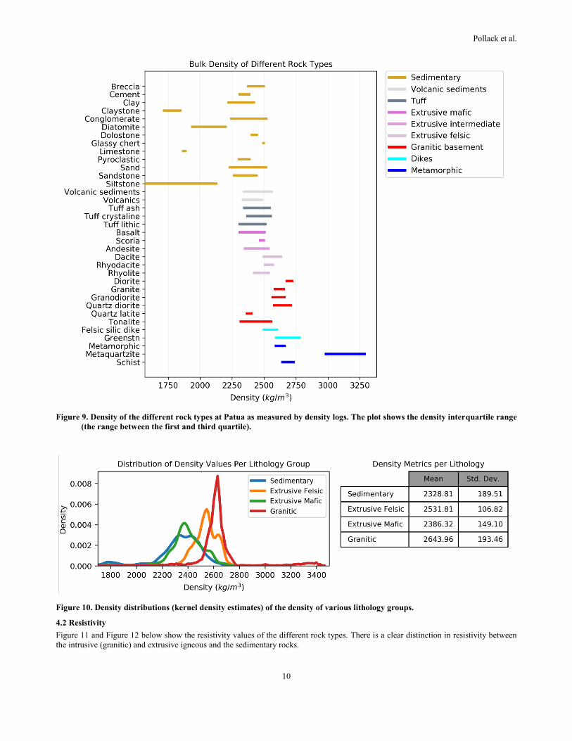
sedimentary rocks, as expected. Figure 10 shows the full distribution of rock properties by lithology type. The uncertainty regarding the

density values is used during the stochastic generation of prior models by sampling density values for the lithology based on the

distributions found in this section.

Pollack et al.

10

Figure 9. Density of the different rock types at Patua as measured by density logs. The plot shows the density interquartile range

(the range between the first and third quartile).

Figure 10. Density distributions (kernel density estimates) of the density of various lithology groups.

4.2 Resistivity

Figure 11 and Figure 12 below show the resistivity values of the different rock types. There is a clear distinction in resistivity between

the intrusive (granitic) and extrusive igneous and the sedimentary rocks.

Pollack et al.

11

Figure 11. Bulk resistivity of different rock types.

Figure 12. Distribution of log resistivity values of different rock types.

5. PARAMETERIZATION OF THE PRIOR MODELS USING PYNODDY

One of the most crucial steps for creating prior models is finding a software that can generate geologically realistic subsurface models as

well as parameterizing the structural model using such a software.

Pollack et al.

12

5.1 Comparison of methods for generating stochastic geomodels

There are six distinct methods for generating realizations of structural models and different features available in each method (Table 1).

Four capabilities are analyzed for each method. The first distinguishing feature is the potential for creating faults. Many methods create

smooth realizations of the subsurface and cannot generate discontinuities. For example, Sequential Gaussian Simulation does not

produce discontinuities. The second feature is the ability to create balanced cross-sections, which means that the rock volume of the

different layers following deformation should be close to the rock volume before deformation. For example, in the case of faulting, the

rock layers should be displaced due to faulting based on the slip. Methods such as multiple point statistics or methods based on a

potential field or object placement do not simulate geologic events and thus cannot ensure that structural models can be restored to

geologically reasonable models; these methods cannot ensure a balanced geologic section.

The third feature reviewed is the ability to create geologically reasonable fault configurations. A balanced geologic section is only one

element of ensuring geologic realism. Faults also need to have reasonable slip values, ratios of slip to fault length, geometries, and

properties that make mechanical sense when considering interactions with nearby faults and general tectonic setting at the simulated

location. Kinematic methods for example, can ensure balanced geologic sections, but cannot ensure geologically reasonable input

parameters.

The final feature reviewed (Table 1) is the ability to condition the realization to data. The ultimate goal of the modelling process is to

create a geomodel that matches observed data. Some methods can utilize observed data in the simulation process and generate

realizations that already match some of the collected data. For example, Sequential Gaussian Simulation, multiple point statistics, and

potential field methods can respect lithology data collected in the wellbore as part of the algorithm process. Sequential Gaussian

Simulation and multiple point statistics methods can also respect information from geophysical methods in the form of lithology

probability cubes. Potential-field based methods, such as GemPy (De La Varga et al., 2019) can also respect lithology dip indicators. On

the other hand, kinematic methods, object-based methods and process-based methods cannot automatically condition to data. However,

if these methods generate simulations with very fast computation time, then stochastic inversion methods could be utilized to perform

the inversion.

For this work, we used the kinematic structural modeling approach. This method strikes a balance between geologic realism and

computational speed that allows for quickly sampling from the prior distribution for Bayesian parameter estimation.

5.2 General description of PyNoddy capabilities

We used the software PyNoddy (Wellmann et al., 2016), which is a python wrapper for the software Noddy (Jessell & Valenta, 1996),

which can be used to simulate faulting, folding, strain, shearing, rotation, dykes, and other geological events. The Noddy algorithm

works by starting with a definition of a flat stratigraphy, which is then discretized into 25 to 250 m cubes, and then applying a series of

geologic deformation events to this discretized space. This process ensures that the final geomodel is a balanced section. In addition,

PyNoddy can also forward-simulate the gravity and magnetic signature of the geomodel based on the provided density, resistivity and

geophysical survey parameters.

The geomodel realizations are created by defining the stratigraphy and then a set of faulting events. The faulting events are defined by

providing the fault location, deformation ellipse properties, and maximum slip quantity. An online notebook with examples of

generating the prior models for this paper can be found by clicking the following link:

https://mybinder.org/v2/gh/ahinoamp/Stochastic-GeoModel-Patua-SGW/master?filepath=MainScript.ipynb.

5.3 Heuristics for geologic realism when using PyNoddy

One of the downsides of using Noddy instead of a process-based method is that the software does not ensure geologic realism, beyond

creating a balanced section. Geologic events defined in Noddy can be non-realistic. For example, it is possible to input into Noddy a

fault slip value that is larger than the fault length value, while such a scenario does not exist in nature. To address this challenge, it is

possible to impose heuristics, or rules, as to allowed values and combination of values in the definitions of geologic events in the input

file to make geomodels more geologically realistic. We present here two proposed rules:

1. Faults should not have a constant displacement across their surface, but rather should be defined as elliptic or curved faults,

where the displacement (slip) is maximal at the center and diminishes towards the edges.

2. The fault slip should be reasonable given the fault length.

Elliptical faults

Researchers widely accept that faults have elliptic displacement patterns, where displacement is maximal at the center of the fault, and

diminishes to zero at the edges of the fault, following an ellipsoidal shape (Kim & Sanderson, 2005), see Figure 13. Noddy has the

option to generate not only planar faults, with constant displacement across a surface, but also elliptic faults. This option should be used

for all input faults to preserve geologic realism.

Pollack et al.

13

Table 1. Different geomodel generation algorithms. The example multiple point statistics image is modified from Liu et al.

(2009). The example potential field method realization is modified from De La Varge et al. (2019). The example process

based method is modified from Finch and Gawthorpe (2017).

Method Description

Ability to model

structural

elements

(faults/folds)

Create balanced

geological section

Create

geologically

reasonable fault

configurations

Ability to

condition the

model to data?

Example

realization image

Sequential

Gaussian

Simulation

Spatial Monte

Carlo sampling

based on a

variogram

No

Cannot model

structural

discontinuous

elements

No No Yes

Conditions to log

data and probability

cubes

Multiple

point

statistics

Creates models

that resemble an

input pattern

Somewhat

No No Yes

Conditions to log

data and probability

cubes

Potential-

field (e.q.

GemPy)

Interpolates

structures

between input

points

Yes No

Does not respect

the offset of

stratigraphic layers

due to fault slip

No Yes

Conditions to log

data and lithology

orientations

Object

based (e.q.

discrete

fracture

networks)

Stochastically

placing faults or

lithological units

in the subsurface

Yes No Does not respect

the offset of

stratigraphic layers

due to fault slip

No No Does not have

conditioning ability,

but simulation time

is sufficiently fast to

perform MCMC

Kinematic

structural

modeling

(e.q.

PyNoddy)

Uses kinematic

equations to

simulate a series

of geologic

events

Yes Yes No

There is no

physical limitation

on fault offsets or

overall

configurations

No Does not have

conditioning ability,

but simulation time

is sufficiently fast to

perform MCMC

Process

based (e.q.

discrete

element

methods)

Numerical

simulations of

deformation

processes

Yes Yes Yes No Does not have

conditioning ability,

and is too slow to

use stochastic

inversion methods

Figure 13. (a) Example of the parameterization of an elliptic fault, where fault displacement diminishes outwards according to a

shape of an ellipsoid. The dark gray color in the center of the deformation ellipsoid on the fault indicates the area with

the highest displacement, and the outer light gray ellipsoid indicates an area with reduced displacement. 𝐞𝐰 is the

ellipsoid width, and 𝐞𝐡 is the ellipsoid height.

Pollack et al.

14

Realistic fault slip relative to the fault length

There is a relationship between fault length and fault displacement: larger faults have larger displacement and vice versa. Kim and

Sanderson (2005) find the maximum fault displacement relates to the length of the fault via the following equation:

𝑑𝑚𝑎𝑥 = 𝑐𝐿𝑛 (1)

Where 𝑑𝑚𝑎𝑥 is the maximum displacement, 𝑐 is a constant, 𝐿 is the fault length, and 𝑛 is an exponent. Often, an exponent of n=1 is

observed in field studies (Kim & Sanderson, 2005), leading to a linear relationship between the maximum fault displacement and the

fault length, as shown in Figure 14. For normal-fault settings, this ratio between maximum fault displacement and fault length is

typically between 0.001 and 0.1, based on several studies aggregated by Kim and Sanderson (2005). In our modeling workflow, we are

only representing faults with a length between 100 and 10,000 m and therefore the slip values should always fall within the gray zone

indicated in Figure 14.

Figure 14. Relationship between fault length and maximum fault displacement. The solid lines show the relationship between

fault length and fault displacement following the equation: 𝒅𝒎𝒂𝒙 = 𝒄𝑳𝒏, when 𝒏 = 𝟏, and 𝒄 =𝒅𝒎𝒂𝒙

𝑳, and given different

values of 𝒅𝒎𝒂𝒙

𝑳. The red dashed line showed the relationship observed in a study by Wells and Coppersmith (1994). The

gray zone indicates points with acceptable values of slip given the fault length for our study.

5.4 Computational cost of PyNoddy simulations

The Bayesian inversion workflow necessitates that the geomodel generation step and gravity simulation step run quickly in order to

converge to realizations that fit the observed data. We see in Figure 15 that the computation time for the geomodel and gravity field is

less than a minute so long as the cell size is less than 50 meters, which is sufficiently quick for stochastic inversion methods.

Figure 15. Computation time for a single PyNoddy geomodel realization.

Pollack et al.

15

6. PRIOR MODEL SCENARIOS FOR PATUA

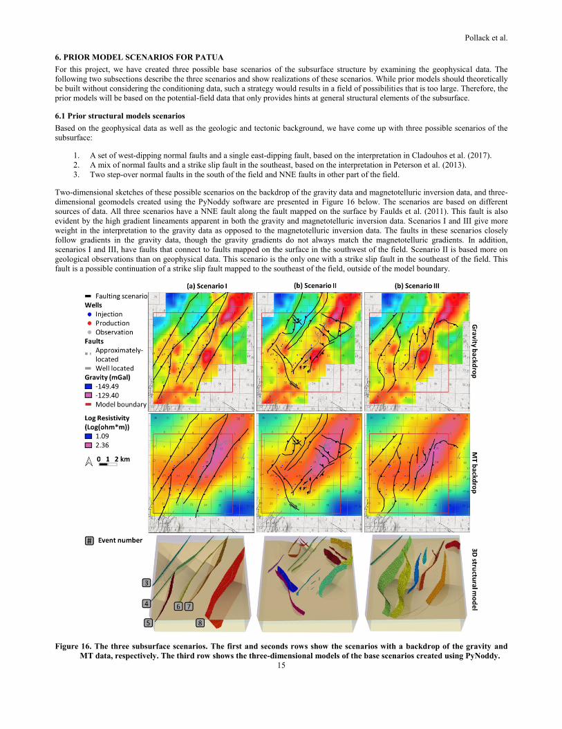
For this project, we have created three possible base scenarios of the subsurface structure by examining the geophysical data. The

following two subsections describe the three scenarios and show realizations of these scenarios. While prior models should theoretically

be built without considering the conditioning data, such a strategy would results in a field of possibilities that is too large. Therefore, the

prior models will be based on the potential-field data that only provides hints at general structural elements of the subsurface.

6.1 Prior structural models scenarios

Based on the geophysical data as well as the geologic and tectonic background, we have come up with three possible scenarios of the

subsurface:

1. A set of west-dipping normal faults and a single east-dipping fault, based on the interpretation in Cladouhos et al. (2017).

2. A mix of normal faults and a strike slip fault in the southeast, based on the interpretation in Peterson et al. (2013).

3. Two step-over normal faults in the south of the field and NNE faults in other part of the field.

Two-dimensional sketches of these possible scenarios on the backdrop of the gravity data and magnetotelluric inversion data, and three-

dimensional geomodels created using the PyNoddy software are presented in Figure 16 below. The scenarios are based on different

sources of data. All three scenarios have a NNE fault along the fault mapped on the surface by Faulds et al. (2011). This fault is also

evident by the high gradient lineaments apparent in both the gravity and magnetotelluric inversion data. Scenarios I and III give more

weight in the interpretation to the gravity data as opposed to the magnetotelluric inversion data. The faults in these scenarios closely

follow gradients in the gravity data, though the gravity gradients do not always match the magnetotelluric gradients. In addition,

scenarios I and III, have faults that connect to faults mapped on the surface in the southwest of the field. Scenario II is based more on

geological observations than on geophysical data. This scenario is the only one with a strike slip fault in the southeast of the field. This

fault is a possible continuation of a strike slip fault mapped to the southeast of the field, outside of the model boundary.

Figure 16. The three subsurface scenarios. The first and seconds rows show the scenarios with a backdrop of the gravity and

MT data, respectively. The third row shows the three-dimensional models of the base scenarios created using PyNoddy.

Pollack et al.

16

6.2 Generating realization using a “prior uncertainty table” and PyNoddy

There is uncertainty regarding which base scenario is closer to the ground-truth, but there is also uncertainty regarding the properties of

each scenario: such as the fault locations, the fault dip and azimuths, the amount of slip, the fault length, as well as geological

properties, including the stratigraphy and rock properties, such as density and resistivity. The uncertainty regarding these properties is

defined in “prior uncertainty table” by specifying the distribution of possible values for these properties. An example of such a table for

the first base case scenario is shown in Table 2.

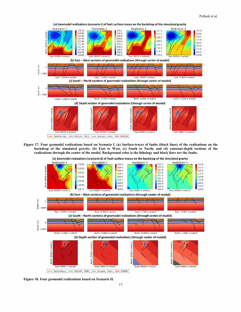
By sampling values from the distribution of parameters in the prior uncertainty tables, we were able to create realizations of geomodels

using PyNoddy. For example, Figure 17, Figure 18, and Figure 19 show four random realizations of the first, second and third base case

scenarios, respectively. The top row in the figures shows the fault traces on the surface on the backdrop of the simulated gravity data.

Some elements of the simulated gravity in the realization are similar to the true gravity data, shown in Figure 3, but none of the four

random realizations reproduce all of the true gravity structures. During the Bayesian inversion process, we will generate realizations that

better match the collected data.

The second, third, and fourth rows of Figures 17-19 show the East-West, South-North, and constant-depth sections that go through the

center of the model. The fault locations and dips of the realizations within each scenario are different, but also fairly similar to each

other because the distributions of possible input parameters were narrow within each scenario. We kept the parameter ranges small to

preserve the general structure of the scenarios.

The results presented here are the first iteration of the stochastic structural modelling method for the Patua geothermal field. Another

advantage of a Bayesian inversion strategy is that further iterations become easier, allowing the geothermal geoscience team to continue

testing ideas, collaborate and eventually develop a series of statistically-supported models that can be further used to quantify risks of

exploration, and in-field and step-out drilling.

Table 2. Range of property values for the geological and structural events in Scenario I (prior uncertainty table).

Event 1:

Stratigraphy

Layer Density Log(Resistivity) Thickness

Sedimentary 𝑁𝑜𝑟𝑚𝑎𝑙: 𝜇 = 2328 𝜎 = 189

𝑁: 𝜇 = 0.86 𝜎 = 0.46

𝑁: 𝜇 = 150 𝜎 = 20

Volcanic mafic 𝑁: 𝜇 = 2386 𝜎 = 149

𝑁: 𝜇 = 1.09 𝜎 = 0.38

𝑁: 𝜇 = 675 𝜎 = 100

Volcanic felsic 𝑁: 𝜇 = 2531 𝜎 = 106

𝑁: 𝜇 = 1.69 𝜎 = 0.63

𝑁: 𝜇 = 675 𝜎 = 100

Granitic basement 𝑁: 𝜇 = 2643

𝜎 = 193

𝑁: 𝜇 = 2.35 𝜎 = 0.58

Not applicable

Continues until bottom

of model

Event 2: Tilting Tilt: 𝑈[0,5] Tilt direction: 𝑈[310,320]

Dip (°)

Dip

Direction (°) Maximum slip (m) Deformation ellipse radii (m)

Center of

deformation

Event 3: Large

western normal

fault dipping west

𝑈[60,80] 𝑈[290,310] 𝑈[345,435] Length: 𝑈[5164,5707] Width: 𝑈[5164,5707] Outward normal: 𝑈[5164,5707]

X: 𝑈[2079,2339] Y: 𝑈[6566,6826] Z: 𝑈[3870,4130]

Event 4: Large

western normal

fault dipping west

𝑈[60,80] 𝑈[300,320] 𝑈[440,550] Length: 𝑈[6546,7236] Width: 𝑈[6546,7236] Outward normal: 𝑈[6546,7236]

X: 𝑈[3534,3794] Y: 𝑈[5967,6227] Z: 𝑈[3870,4130]

Event 5: Small

SW normal fault

dipping west

𝑈[60,80] 𝑈[274,294] 𝑈[170,215] Length: 𝑈[2569,2840] Width: 𝑈[2569,2840] Outward normal: 𝑈[2569,2840]

X: 𝑈[1396,1656] Y: 𝑈[1766,2026] Z: 𝑈[3870,4130]

Event 6: Medium

fault dipping west

𝑈[60,80] 𝑈[293,313] 𝑈[285,350] Length: 𝑈[4243,4689] Width: 𝑈[4243,4689] Outward normal: 𝑈[4243,4689]

X: 𝑈[4733,4993] Y: 𝑈[4954,5214] Z: 𝑈[3870,4130]

Event 7: Large

eastern fault

dipping west

𝑈[60,80] 𝑈[285,305] 𝑈[360,450] Length: 𝑈[5373,5938] Width: 𝑈[5373,5938] Outward normal: 𝑈[5373,5938]

X: 𝑈[6075,6335] Y: 𝑈[5958,6218] Z: 𝑈[3870,4130]

Event 8: Large

eastern fault

dipping east

𝑈[60,80] 𝑈[111,131] 𝑈[375,470] Length: 𝑈[5557,6142] Width: 𝑈[5557,6142] Outward normal: 𝑈[5557,6142]

X: 𝑈[7435,7695] Y: 𝑈[4585,4845] Z: 𝑈[3870,4130]

Pollack et al.

17

Figure 17. Four geomodel realizations based on Scenario I. (a) Surface-traces of faults (black lines) of the realizations on the

backdrop of the simulated gravity. (b) East to West, (c) South to North, and (d) constant-depth sections of the

realizations through the center of the model. Background color is the lithology and black lines are the faults.

Figure 18. Four geomodel realizations based on Scenario II.

Pollack et al.

18

Figure 19. Four geomodel realizations based on Scenario III.

6.3 Visualizing structural uncertainty

We are able to visualize the structural uncertainty by combining the faults from the different realizations within each scenario. Figure

20 shows East to West cross-sections of the faults and top of the stratigraphic layers for twenty realizations based on each of the three

scenarios. The spatial spread of the faults visualizes the uncertainty regarding the faults’ dips, lengths and locations. Figure 20 provides

an example of how to visualize uncertainty, an important element of a stochastic workflow. Geoscientists can use such figures to

communicate the implications of structural uncertainty. For example, Figure 20 can be used to show the uncertainty of fault location

when designing a wellbore trajectory that targets one of the faults.

Figure 20. East to West cross-sections of twenty geomodel realizations based on (a) Scenario I, (b) Scenario II, and (c) Scenario

III. Black semi-transparent lines indicate faults. Gray, purple and red lines indicate the tops of the stratigraphic layers.

Figure 21 shows the full uncertainty when considering all three scenarios. The different colors of the faults represent faults from

different scenarios. In all of the scenarios, there is an east-dipping fault on the east of the section, and therefore there is a fair amount of

certainty regarding that fault event even before performing a Bayesian inversion. On the other hand, there is significant variability

between scenarios regarding fault geometry on the western part of the section. We will be reducing this uncertainty in the next step of

the Bayesian inversion process.

Pollack et al.

19

Figure 21. East to West cross-section of twenty geomodel realizations based on each scenario. Brown lines represent faults based

on Scenario I, blue lines represent faults based on Scenario II, and green lines represent faults based on Scenario III.

Gray, purple and red lines indicate the tops of the stratigraphic layers.

CONCLUSIONS

Bayesian inversion strategies have two central advantages compared to manual expert interpretations of the subsurface. First,

researchers can generate multiple geomodels of the subsurface and quantify the uncertainty regarding different structures. Second, the

computational nature of Bayesian methods allows for consistency with a larger portion of collected geophysical, geological, and well

testing datasets. In addition, the fit between different geomodels and the datasets can be quantified.

In order to perform a Bayesian workflow, geoscientists need to parameterize the geomodel and define the prior uncertainty regarding the

different elements in the subsurface model. In this paper, we provide a case study of performing this step of defining prior uncertainty

for Cyrq Energy’s Patua Geothermal Field. Based on the regional tectonic patterns and potential-field data, we find that Patua may be

expected to have north-northeast normal faulting structures in the north of the field and possibly some east-west or northwest strike-slip

structures in the south of the field. The subsurface well log data indicate four main layers: sedimentary cover, mafic volcanic rock, felsic

volcanic rock, and granitic basement. Using this background information, we created three base case scenarios of the lithology and

faulting structures at Patua. We used the kinematic simulator, Noddy, via a python wrapper, PyNoddy, to generate geomodel

realizations based on the base-case scenarios. The values for each structural simulation input parameter were sampled from a

distribution defined in a prior uncertainty table. Noddy simulates the realizations quickly enough for using this prior model generation

process in a future implementation of a full Bayesian inversion workflow.

A binder notebook, https://mybinder.org/v2/gh/ahinoamp/Stochastic-GeoModel-Patua-SGW/master?filepath=MainScript.ipynb, is

available for readers to view the geomodels in this paper and generate their own geomodels.

ACKNOWLEDGEMENTS

We would like to thank Drew Siler and Jim Faulds for giving advice on this paper.

REFERENCES

Brown, D. W., Duchane, D. V., Heiken, G., & Hriscu, V. T. (2012). Minning the Earth’s Heat: Hot Dry Rock Geothermal Energy. New

York: Springer. https://doi.org/10.1007/978-3- 540 -68910-2_1

Cladouhos, T. T., Uddenberg, M. W., Swyer, M. W., Nordin, Y., & Garrison, G. H. (2017). Patua geothermal geologic conceptual

model. Transactions - Geothermal Resources Council, 41, 1057–1075.

Faulds, J. E., & Henry, C. D. (2008). Tectonic influences on the spatial and temporal evolution of the Walker Lane : An incipient

transform fault along the evolving Pacific – North American plate boundary. Ores and Orogenesis: Circum- Pacific Tectonics,

Geologic Evolution, and Ore Deposits, Arizona Ge, 437–470.

Faulds, J. E., & Hinz, N. H. (2015). Favorable Tectonic and Structural Settings of Geothermal Systems in the Great Basin Region ,

Western USA: Proxies for Discovering Blind Geothermal Systems. World Geothermal Congress 2015, (April), 1–6.

Faulds, J. E., Coolbaugh, M. F., Benoit, D., Oppliger, G., Perkins, M., Moeck, I., & Drakos, P. (2010). Structural Controls of

Geothermal Activity in the Northern Hot springs Mountains, Western Nevada: The Tale of Three Geothermal Systems (Brady’s,

Desert Peak, and Desert Queen). In GRC Transactions.

Faulds, J. E., Ramelli, A. R., & Perkins, M. E. (2011). Preliminary Geologic Map of the Hazen Quadrangle, Lyon and Churchill

Counties, Nevada. Retrieved from https://pubs.nbmg.unr.edu/Prelim-geologic-Hazen-quad-p/of2011-08.htm

Faulds, J. E., Hinz, N. H., Dering, G. M., & Siler, D. L. (2013). The hybrid model - The most accommodating structural setting for

geothermal power generation in the Great Basin, western USA. Transactions - Geothermal Resources Council, 37(PART 1), 3–10.

Finch, E., & Gawthorpe, R. (2017). Growth and interaction of normal faults and fault network evolution in rifts: Insights from three-

dimensional discrete element modelling. Geological Society Special Publication, 439(1), 219–248.

https://doi.org/10.1144/SP439.23

Pollack et al.

20

Jessell, M. W., & Valenta, R. K. (1996). Structural geophysics: Integrated structural and geophysical modelling. Computer Methods in

the Geosciences, 15(C), 303–324. https://doi.org/10.1016/S1874-561X(96)80027-7

Kim, Y. S., & Sanderson, D. J. (2005). The relationship between displacement and length of faults: A review. Earth-Science Reviews,

68(3–4), 317–334. https://doi.org/10.1016/j.earscirev.2004.06.003

De La Varga, M., Schaaf, A., & Wellmann, F. (2019). GemPy 1.0: Open-source stochastic geological modeling and inversion.

Geoscientific Model Development, 12(1), 1–32. https://doi.org/10.5194/gmd-12-1-2019

Liu, X., Zhang, C., Liu, Q., & Birkholzer, J. (2009). Multiple-point statistical prediction on fracture networks at Yucca Mountain.

Environmental Geology, 57(6), 1361–1370. https://doi.org/10.1007/s00254-008-1623-3

Lund Snee, J.-E., & Zoback, M. D. (2020). Multiscale variations of the crustal stress field throughout North America. Nature

Communications.

Peterson, N., Combs, J., Bjelm, L., Garg, S., Kohl, B., Goranson, C., et al. (2013). Integrated 3D Modeling of Structural Controls and

Permeability Distribution in the Patua Geothermal Field, Hazen, NV. In Thirty-Eighth Workshop on Geothermal Reservoir

Engineering at Stanford University.

Scheidt, C., Li, L., & Caers, J. (2018). Quantifying Uncertainty in Subsurface Systems. American Geophysical Union. Hoboken, NJ,

USA: John Wiley & Sons, Inc. https://doi.org/10.1029/2011GM001187.Cited

U.S. Geological Survey. (2006). Quaternary fault and fold database for the United States. Retrieved October 28, 2019, from

https://earthquake.usgs.gov/hazards/qfaults/

Wellmann, J. F., Thiele, S. T., Lindsay, M. D., & Jessell, M. W. (2016). Pynoddy 1.0: An experimental platform for automated 3-D

kinematic and potential field modelling. Geoscientific Model Development, 9(3), 1019–1035. https://doi.org/10.5194/gmd-9-1019-

2016

Wells, D. L., & Coppersmith, K. J. (1994). New empirical relationships among magnitude, rupture length, rupture width, rupture area,

and surface displacement. Bulletin - Seismological Society of America, 84(4), 974–1002.