STOCHASTIC SIMULATION OF THE MORPHOLOGY OF FLUVIAL … · morphology of fluvial sand channels...
78
Alexandra Kuznetsova Licenciada STOCHASTIC SIMULATION OF THE MORPHOLOGY OF FLUVIAL SAND CHANNELS RESERVOIRS Dissertação para obtenção do Grau de Mestre em Engenharia Geológica (Georrecursos) Orientador: Doutor José António de Almeida, Prof. Auxiliar – FCT/UNL Co-orientador: Doutor Paulo Alexandre Rodrigues Roque Legoinha, Prof. Auxiliar – FCT/UNL Júri: Presidente: Doutor José Carlos Ribeiro Kullberg, Prof. Auxiliar – FCT/UNL Vogais:Doutora Júlia Cristina da Costa Carvalho, Investigadora. Auxiliar – Cerena/IST-UTL Doutor Martim Afonso Ferreira de Sousa Chichorro, Investigador. Auxiliar – FCT/UNL Doutor José António de Almeida, Prof. Auxiliar – FCT/UNL Doutor Paulo Alexandre Rodrigues Roque Legoinha, Prof. Auxiliar – FCT/UNL June 2012
Transcript of STOCHASTIC SIMULATION OF THE MORPHOLOGY OF FLUVIAL … · morphology of fluvial sand channels...

Alexandra Kuznetsova
Licenciada
STOCHASTIC SIMULATION OF THE
MORPHOLOGY OF FLUVIAL SAND
CHANNELS RESERVOIRS
Dissertação para obtenção do Grau de Mestre em Engenharia Geológica
(Georrecursos)
Orientador: Doutor José António de Almeida, Prof. Auxiliar – FCT/UNL
Co-orientador: Doutor Paulo Alexandre Rodrigues Roque Legoinha, Prof. Auxiliar –
FCT/UNL
Júri:
Presidente: Doutor José Carlos Ribeiro Kullberg, Prof. Auxiliar – FCT/UNL
Vogais:Doutora Júlia Cristina da Costa Carvalho, Investigadora. Auxiliar –
Cerena/IST-UTL
Doutor Martim Afonso Ferreira de Sousa Chichorro, Investigador. Auxiliar –
FCT/UNL
Doutor José António de Almeida, Prof. Auxiliar – FCT/UNL
Doutor Paulo Alexandre Rodrigues Roque Legoinha, Prof. Auxiliar – FCT/UNL
June 2012
i
STOCHASTIC SIMULATION OF THE MORPHOLOGY OF FLUVIAL
SAND CHANNELS RESERVOIRS
Copyright em nome de Alexandra Kuznetsova, da FCT/UNL e da UNL
A Faculdade de Ciências e Tecnologia e a Universidade Nova de Lisboa tem o direito, perpétuo e
sem limites geográficos, de arquivar e publicar esta dissertação através de exemplare impressos
reproduzidos em papel ou de forma digital, ou por qualquer outro meio conhecido ou que venha a
ser inventado, e de a divulgar através de repositórios científicos e de admitir a sua copia e
distribuição com objectivos educacionais ou de investigação, não comerciais, desde que seja dado
crédito ao autor e editor.

ii
Acknowledgments
I am sincerely and heartily grateful to Doctor José António de Almeida and Doctor Paulo Legoinha
for the idea to write this work, for possibility to work with them and also for guiding and correcting
with attention and care throughout my thesis writing.
This master's thesis is supported by the Erasmus Mundus Action 2 Programme of the European Union.

iii
Resumo
A caracterização de reservatórios de petróleo de tipo fluvial com algoritmos estocásticos constitui
um problema complexo. Isto porque os canais apresentam padrões espaciais que não são
caracterizados pelas estatísticas bi-ponto que estão na base dos modelos geoestatísticos. Entre estes
aspectos contam-se, por exemplo, as morfologias deltaica, meandriforme e de planície aluvial, onde
os canais formam um complexo padrão 3D resultante da acumulação de sedimentos pela antiga
rede fluvial.
No presente trabalho apresenta-se uma metodologia inovadora destinada a gerar imagens da
morfologia de canais arenosos em reservatórios fluviais, com base em um modelo de simulação
3D. É baseada nas seguintes etapas: (1) partir de histogramas do comprimento, largura e altura de
canais de areia, e de um malha de pontos com orientações locais; (2) fazer a simulação estocástica
das dimensões largura e altura de hipotéticos canais de areia (3) gerar e posicionar esqueletos de
hipotéticos canais e associar as dimensões largura e altura geradas na etapa anterior (modelo
booleano estocástico de tipo vectorial); (4) converter o modelo anterior para um modelo matricial,
associando zonas com diferenciação da incerteza; (5) utilização do método de simulação de campos
de probabilidade (probability field simulation – PFS) para pós-processar o modelo booleano na
forma matricial obtido na etapa anterior. Os resultados do modelo são várias imagens
equiprováveis binárias (canal / não canal) que podem posteriormente ser preenchidas por valores de
porosidade e permeabilidade.
Esta metodologia foi testada com sucesso para a modelação de canais de areia de um reservatório
fluvial do médio oriente. Concretamente, discutem-se os resultados do modelo obtido, faz-se uma
análise do padrão de formas obtido na relação com a imagem de orientações locais de partida e
tecem-se comentários sobre a incerteza local e global do modelo em função da conectividade dos
canais.
Palavras-chave: reservatórios fluviais; canais de areia; geoestatística; modelos booleanos;
modelos estocásticos.
iv
Abstract
The characterization of fluvial-type oil reservoirs using stochastic simulation algorithms is a
complex problem because the morphology of the channels are complex and are not fully
characterized by the two-point statistics of the geostatistical models (variograms and/or spatial
covariances). Among these features, for example, are delta morphologies and meander-form
floodplain where the channels form a complex pattern of the resulting 3D sediment accumulation
by the former waterway system.
This work presents an innovative methodology designed to simulate 3D stochastic images of the
morphology of fluvial sand channels reservoirs. It is based on the following steps: (a) preparation
of histograms of length, width and height of sand channels and a 2D image of local orientations; (2)
simulate widths and heights of the hypothetical sand channels along their paths; (3) generate
randomly skeletons of hypothetical channels and associate the width and height dimensions
generated in the previous step (Boolean vector model); (4) convert the Boolean vector model into a
raster model and link regions of uncertainty according distances to the skeleton; (5) finally, using
the method of Probability Field Simulation (PFS) condition the Boolean model with a model of
variogram and resolve the regions of uncertainty. The outputs are sets of binary images (channel –
sand / not channel – shale) that can be filled by values of porosity and permeability.
This methodology was successfully tested for modeling channel sand reservoir of a river of the
Middle East. Specifically, results are discussed in connection with the image of local orientations
together with an analysis of the local and global uncertainties of the model.
Keywords: fluvial reservoirs; sand channels; geostatistics; Boolean models; stochastic models.
v
Contents
1. INTRODUCTION ....................................................................................................... 1
1.1 Organization of the thesis ............................................................................................ 3
2. GEOLOGICAL ENVIRONMENT……………………………………………………4
2.1 Types of sedimentary rocks ......................................................................................... 4
2.2 The main parameters of characterization of clastic rocks ............................................ 4
2.2.1 The grain size ................................................................................................................. 4
2.2.2 The grain shape, sphericity and roundness ..................................................................... 6
2.2.3 Sorting of a sediment ...................................................................................................... 7
2.2.4 Porosity and permeability ............................................................................................... 8
2.2.5 Textural maturity ............................................................................................................ 9
2.2.6 Composition ................................................................................................................... 9
2.3 Types of sandstones and geological setting ................................................................. 9
2.4 Types of the rivers and their characteristics ............................................................... 11
2.4.1 Braided rivers ............................................................................................................. 133
2.4.2 Meandering rivers ........................................................................................................ 13
2.4.3 Anastomosed rivers ...................................................................................................... 14
2.4.4 Straight channels .......................................................................................................... 14
2.5 Types of river deposits ............................................................................................... 14
2.6 Facies associations and sedimentary cycles ............................................................... 15
2.7 Tectonic Setting of Fluvial Reservoirs....................................................................... 17
2.8 Styles of Fluvial Reservoir ......................................................................................... 17
2.8.1 Paleovalley Bodies (PV Type) ..................................................................................... 18
2.8.2 Sheet Bodies (SH Type) ............................................................................................... 18
2.8.3 Channel-and-Bar Bodies (CB Type) ............................................................................ 19
2.9 Alluvial sediments...................................................................................................... 19
vi
2.9.1 Alluvial processes ........................................................................................................ 19
2.9.2 Alluvial fans ................................................................................................................. 20
3. PROSPECTION METHODS AND INTEREST VARIABLES……….…………….21
3.1 The use of marker bed ................................................................................................ 21
3.2 Wireline Logs ............................................................................................................. 21
3.3 Lithofacies Mapping .................................................................................................. 22
3.4 Seismic Methods ........................................................................................................ 22
3.5 Ground-Penetrating Radar ......................................................................................... 22
3.6 Magnetostratigraphy .................................................................................................. 23
3.7 Paleocurrent Analysis ................................................................................................ 24
3.8 The Dipmeter ............................................................................................................. 25
3.9 Surveillance Geology ................................................................................................. 26
3.10 Types of data and their applications ..................................................................... 26
4. METHODOLOGY AND THEORETICAL BACKGROUND………...………………28
4.1 Methodology .............................................................................................................. 30
4.2 Background of geostatistics ....................................................................................... 34
4.3 Spatial continuity and variograms .............................................................................. 37
4.3.1 Variogram and spatial continuity ................................................................................. 37
4.3.2 Fitting of theoretical models ........................................................................................ 37
4.4 Simulation strategies .................................................................................................. 38
4.4.1 Sequential simulation methods ..................................................................................... 39
4.4.2 Sequential Gaussian simulation.................................................................................... 41
4.4.3 Direct sequential simulation ......................................................................................... 41
4.4.4 Probability field simulation .......................................................................................... 42
5. CASE STUDY........................................................................................................................45
5.1 Starting data ............................................................................................................... 45
5.2 Stochastic simulation of width and height dimensions .............................................. 47

vii
5.3 Boolean model of the channels .................................................................................. 49
5.4 Probability Field Simulation ...................................................................................... 52
5.5 Porosity simulation constrained to the shale / sand system ....................................... 55
5.6 Reservoir and potential OIP evaluation ..................................................................... 56
5.7 Discussion .................................................................................................................. 58
6. FINAL REMARKS.................................................................................................... 63
7. REFERENCES........................................................................................................... 64
viii
Figures
Figure 1 - Schematic view of the different scale and type of heterogeneities that can affect fluid
flow behaviour in fluvial depositional systems (modified from Weber, 1986).................................. 3
Figure 2.2.1 – Classification of sedimentary particles based on Wentworth’s classification of grain
size (Fritz, Moore, 1988)..............................................................................................................…...5
Figure 2.2.2 – Triangle diagram, illustrating the names, given to various shapes of sedimentary
particles, based on a method by Sneed and Folk (1958) ……………………………………….…...6
Figure 2.2.3 – Diagram illustrating the equivalent sieve diameter of different shaped grains (Fritz,
Moore, 1988)………………………………………………………….…………………………..…7
Figure 2.2.4 – Sorting and grain size distribution for sediments from a variety of environments.
(From Folk, 1974)…………………………………………………….…….………………………..7
Figure 2.5 – An example of some type of porosity (Basic Petroleum Geology and Log Analysis,
2001)………………………………………………………………….…………………..………….8
Figure 2.2.5 – Figure for estimating percentage of a component by volume (Compton, 1985)…...10
Figure 2.4.1 – Sketches to show the range of river channel types (adapted after Brice, 1984)……11
Figure 2.4.2 – Channel types related to the dominant type of bedload in the stream and the relative
stability of channel banks (after Orton & Reading, 1993)……………………...…….…………….12
Figure 2.4.3 – a) Braided river, Denali National Park, Alaska (Walsh, 2007); b) meandering river,
Williams river, Alaska (Smith, 2007); c) anastamosed river, avulsion belt of the Saskatchewan
River (Smith, 2007); d) straight river, Kaa-Khem River, Siberia, Russia (Reuters, 2008)……..….13
Figure 2.5.2 - Development of a fining-upward succession by lateral accretion of a point bar, such
as that in figure 2.5.1b (Miall, 2008). ............................................................................................... 15
Figure 2.6.1 – Facies model for the Battery Point Sandstone based on analysis of vertical facies
transitions through many channel units. The model presents an ideal that is seldom complete in
nature (after Cant & Walker, 1976)…………………………………….……….………………… 16
Figure 2.8.1 – Classification of nonmarine reservoirs according to the geometry of the depositional
system and the geometry of the reservoir body………………………..……….…………………..18
Figure 3.4.1 – Horizontal slice section, part of 3-D seismic section showing bifurcating deltaic
distributaries, Cenozoic, Gulf of Mexico (Brown, 1991)……………….……….…………………23
Figure 3.6.1 – Magnetic sampling of fluvial succession, the Miocene-Pliocene Siwalik Group of
Pakistan. Black sample points, normal polarity, open points, reserved polarity (Behrensmeyer and
Tauxe, 1982)………………………………………………………………………………………..24
ix
Figure 3.8.1 – Typical point bar and the dipping surface associated with it. The speculative
dipmeter log is also shown………………………………………………….………….…………..25
Figure 3.9.1 – Use of pressure-depth plot to test lithographic correlation. The points fall into 2
groups, indicating that they represent 2 channel-fill sandstone bodies isolated from each other by
fine-grained units. Mannville Sandstone, Alberta (Putnam and Oliver, 1980)………....………….26
Figure 4.1 – Workflow of the proposed methodology. .................................................................... 30
Figure 4.2 – Example of an image of local orientations (azimuths). ............................................... 31
Figure 4.3 – Generation of a 3D channel: (left) simulation of the skeleton; (right) assign local
widths and heights. ........................................................................................................................... 32
Figure 4.4 – Transformation from vector to raster and generation of three a priori regions (sand,
transition and shale). ........................................................................................................................ 33
Figure 4.5 – (top left) Simulated image of gaussian values conditioned to local ellipsoid
orientations ; (top right) Homologous probability field simulated image; (bottom) local ellipsoid
orientations (only for illustrative purposes, no correspondence with the top images). .................... 43
Figure 5.1 – Cumulative histograms of the length, width and height dimensions. .......................... 46
Figure 5.2 – Flow direction angles or local orientation of the potential flow (Aljustrel, Alentejo). 46
Figure 5.3 – Flowdirection angles after smoothing and reclassification. ......................................... 47
Figure 5.4 – (left) Simulated values of widths for 250 channels; (right) simulated values of heights
for 250 channels. .............................................................................................................................. 48
Figure 5.5 – (left) Simulated values of widths for 500 channels; (right) simulated values of heights
for 500 channels. .............................................................................................................................. 48
Figure 5.6 – (top) Two simulations of skeletons for 250 channels; (bottom) correspondent 3 regions
block models (blue – sand; red – transition sand/shale). .................................................................. 49
Figure 5.7 – (top) Two simulations of skeletons for 500 channels; (bottom) correspondent 3 regions
block models (blue – sand; red – transition sand/shale). .................................................................. 50
Figure 5.8 – (top) Two simulations of skeletons for 500 channels; (bottom) correspondent 3 regions
block models (blue – sand; red – transition sand/shale) with width subdivided by two. ................. 50
Figure 5.9 – Examples of two simulated probability images used for PFS purposes. ..................... 52
Figure 5.10 – Examples of two simulated images of the morphology of the sand / shale system for
250 channels. .................................................................................................................................... 53

x
Figure 5.11 – Examples of two simulated images of the morphology of the sand / shale system for
500 channels (initial width). ............................................................................................................. 54
Figure 5.12 – Examples of two simulated images of the morphology of the sand / shale system for
500 channels (width / 2). .................................................................................................................. 54
Figure 5.13 – Cumulative histograms for porosity conditioned to sand and shale facies. ............... 55
Figure 5.14 – Examples of three simulated images of porosity constrained to the morphology of the
sand / shale system for 250 channels, 500 channels and 500 channels with half width. .................. 56
Figure 5.15 – Potential OIP curves the 250 channels scenario. ....................................................... 57
Figure 5.16 – Potential OIP curves the 500 channels scenario. ....................................................... 57
Figure 5.17 – Potential OIP curves the 500 channels, width /2 scenario. ........................................ 57
Figure 5.18 – Comparative results of one simulated image for (left) level and (right) cross-section
for scenario of 250 channels............................................................................................................. 58
Figure 5.19 – Comparative results of one simulated image for (left) level and (right) cross-section
for scenario of 500 channels............................................................................................................. 59
Figure 5.20 – Comparative results of one simulated image for (left) level and (right) cross-section
for scenario of 500 channels and width / 2. ...................................................................................... 60

xi
Tables
Table 2.8 – The three major types of petroleum reservoir in fluvial sandstones (Miall, 1996)…....17
Table 4 – Comparison of modelling approaches…………………………………………………...28
Table 5.1 – Parameters of the synthetic reservoir grid blocks. ........................................................ 45
Table 5.2 – Average dimensions of the channels. ............................................................................ 48
Table 5.3 – Proportions of the different regions (shale, sand, and transition shale-sand) by
realization, scenario of 250 channels. .............................................................................................. 51
Table 5.4 – Proportions of the different regions (shale, sand, and transition shale-sand) by
realization, scenario of 500 channels. .............................................................................................. 51
Table 5.5 – Proportions of the different regions (shale, sand, and transition shale-sand) by
realization, scenario of 500 channels, width / 2. .............................................................................. 52
Table 5.6 – A priori probabilities of each region being sand / shale. ............................................... 53
Table 5.7 - Statistic results of the sixty simulated images, scenario of 250 channels (PFS). ........... 53
Table 5.8 - Statistic results of the sixty simulated images, scenario of 500 channels (PFS). ........... 54
Table 5.9 - Statistic results of the sixty simulated images, scenario of 500 channels, width / 2
(PFS). ............................................................................................................................................... 55

1
1. INTRODUCTION
The intensive and growing exploration of petroleum from reservoirs in the last decades, associated
with a decrease of reserves, focus the interest in research and characterization steps which became
more complex and expensive, raising the magnitude of risk decisions.
The main objective of the evaluation of petroleum reservoirs is forecasting production of oil and/or
gas, including reserves assessment (potential oil in place) and the location of new wells. This
involves modelling the fluid flow, which requires first modelling of petrophysical properties such
as porosity and permeability. The petrophysical properties often differ between facies and therefore
should be modelled separately for each facies, which means that modelling should be a two-step
methodology, beginning with the morphology and followed by the properties simulated
conditionally to the facies model. To this end, it is necessary a good model for the distribution of
the reservoir facies (morphological model).
Fluvial reservoirs offer a particular challenge for modelling (Luis and Almeida, 1997) due to their
variable geometries and complex networks. In particular fluvial sands reservoirs are characterized
by their elongate shapes with a relatively small width-length ratio. In this regard, a very topical
issue is the development of theoretical and methodological principles of using computer technology
for resolving problems of prospecting and exploration of oil and gas for fluvial reservoirs.
Nowadays there are a lot of different approaches of modelling. There is no unique or ‘best’
approach that would be valid for all reservoirs of all types. In order to visualize reservoirs with
complicated structures it is better to mix some of them. The choice of the “best” methodology
always depends on geological, morphological and structural conditions, as well as data available.
Stochastic models of reservoirs are an important tool for assessing geological heterogeneity
conditioned to different sources and detail of the available data, at all steps of reservoir
development: discovery, evaluation of reserves, exploitation, enhanced recovery and closure. There
are many techniques and methodologies for reservoirs modelling, but regarding the small amount
of data they are typically simulation based (Deutsch and Journel, 1992; Almeida, 1999; Vargas-
Guzmnan and Al-Qassab, 2006; Mata-Lima, 2008).
As it is known, oil and gas with commercial interest only exist in certain regions and under special
conditions. Rocks in suitable stratigraphic positions, possessing porosity and permeability able to
contain oil, or gas, or both in commercial quantities, are named reservoir rock. The most common
types of reservoir rocks are clastic sediments (sandstones, conglomerates) and grained or
crystalline carbonate rocks. This work deals with the particular class of clastic sediments, namely
fluvial rocks.
1. Introduction
2
The fluvial reservoirs represent about 20% of the world’s remaining reserves of hydrocarbons, and
are indeed an important reservoir type for the petroleum industry (Keogh et al, 2007). For a long
time in petroleum reservoir description the modelled sedimentary deposits were represented as
totally homogeneous bodies, both with regards to sedimentological and structural heterogeneities,
in a gross simplification of their potential flow behaviour.
The aim of reservoir simulation models is to integrate data from multiple scales of measurement to
capture a geologically realistic range and spatial variability in petrophysical properties, so as to be
able to realistically simulate flow through them, as well as to be able to predict future oil and gas
production of alternative recovery scenarios and to optimize field development.
The discovery of potentially large hydrocarbon accumulations within fluvial deposits in the
Norwegian North Sea in the late 1970's to early 1980's, many fields in the Pennsylvanian Cherokee
Group of Kansas, several fields in the Upper Pennsylvanian and Lower Permian on the eastern
shelf of the midland Basin in West Texas, the upper part of the Sadlerochit formation at Prudhoe
Bay in Alaska, the Upper Triassic sands in the Rankin gas fields on the northwest shelf of
Australia, the approximately coeval sandstones in the Morecambe gas field of north-western
England, all or most of the tar sands in the Uinta Basin of the USA (North, 1985) led to the
realization that to produce these deposits economically and effectively, better prediction of their
connectivity and flow behaviour requires the development of special modelling algorithms.
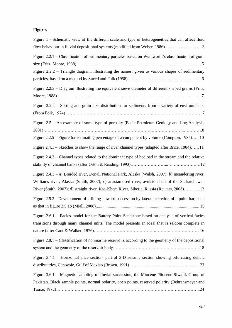
A wealth of sedimentary studies on outcrops and modern systems had already identified that fluvial
deposits are heterogeneous on a variety of scales, from the microscopic to the megascopic scale
(figure 1).
To better characterize these reservoir types and extract hydrocarbons it is important to understand
the occurrence and variability of these various scales of heterogeneities. Also, predict
heterogeneities caused by faulting are equally important in fluvial reservoirs characterization.
For modelling this type of reservoirs two approaches are currently used: Boolean and multi-point.
In Boolean modelling channels are positioned in the volume under study in a deterministic or
stochastic design of the skeleton of the channel. In the case of a deterministic positioning, one
digitizes the position of the skeleton on 2 or 3D set (a range of arcs) based, for instance, on a
seismic image. On the base of a skeleton is generated the channel’s form after appropriation of a
width and height throughout the skeleton. The multi-point approach starts from a theoretical or
conceptual image of the shape of channels. From this image is extracted a multi-point statistic of
elementary forms (templates) which are then reproduced by simulation in new images. From a
theoretical standpoint the multi-point approach is effective but has two main problems that is why
it is rarely used in practice: it requires a reference image and is computationally very difficult. The
deterministic approach is thus preferable but in case of post-processed is unrealistic.

1. Introduction
3
Figure 1 - Schematic view of the different scale and type of heterogeneities that can affect fluid
flow behaviour in fluvial depositional systems (modified from Weber, 1986).
1.1 Organization of the thesis
This report is organized into six main sections. This first introduces the challenge of modelling
fluvial sand channels. The second summarize the geological environments of these types of fields
and the third presents some exploration methods and variables of interest. Section 4 describes the
proposed methodology for simulation of fluvial sand channels and section five presents and
discusses an example of channels modelling combining Boolean and stochastic algorithms. Finally,
section 6 presents the final remarks.
2. Geological environments
4
2. GEOLOGICAL ENVIRONMENTS
2.1 Types of sedimentary rocks
To be able to create models of clastic reservoirs it is necessary to understand the geological
environments of the reservoirs. There are two main groups of sedimentary rocks, which are
classified on the basis of their origin:
- Chemical or biochemical;
- Clastic sedimentary rocks.
Also it can be mentioned another classification of sand deposits according to their environments:
Terrestrial (Aeolian or dune sands);
Tidal, deltaic, coastal;
Deep marine and
Fluvial (river deposits).
The most important types of sedimentary rocks in the production of hydrocarbons:
Carbonates;
Shales;
Evaporites;
Sandstones.
This work deals with the particular class of clastic sediments, namely fluvial rocks.
2.2 The main parameters of characterization of clastic rocks
The main characteristics of sedimentary particles can be described by determining their size, shape,
sorting and composition. Size, shape and sorting define the texture.
2.2.1 The grain size
The grain size of the sediment is a function of many interrelated parameters, the most important of
which are: proximity and composition of the source rock, weathering and transport processes and

2. Geological environments
5
physical energy distribution at the site of deposition (Fritz, 1988). The most common grain size
classification is shown on the figure 2.2.1.
Figure 2.2.1 – Classification of sedimentary particles based on Wentworth’s classification of grain
size (Fritz, Moore, 1988).

2. Geological environments
6
2.2.2 The grain shape, sphericity and roundness
Because the shape of sedimentary grains in natural sediment can range it is essential to describe a
shape variation as well. The most common method is a description of sphericity. Actually, the
sphericity measures the equality of 3 mutually perpendicular axes through the grain, presented in
Sneed and Folk’s (1958) formula below: (L) – the length of the long, (I) – intermediate and (S) –
short axes of the grain.
Maximum projection sphericity = S2 / (L I)
These parameters are well represented by a Sneed and Folk’s triangle (figure 2.2.2).
Figure 2.2.2 – Triangle diagram, illustrating the names given to various shapes of sedimentary
particles, based on a method by Sneed and Folk (1958).
One more essential characteristic of sedimentary grains is calculated roundness. Its values range
from 1.0 (perfectly rounded) to approaching 0.0 (very angular). In summary, roundness is a simple
concept: an angular grain bristles with sharp corners and edges, a round displays relatively broad,
smooth surface.

2. Geological environments
7
2.2.3 Sorting of a sediment
Sorting - is a measure of the dispersion of the grain-size distribution of sediment. Because it is very
difficult to determine the grain-size distribution of sediments rapidly, without detailed thin-section
analysis, most sorting determinations are made by comparison to a standard drawing.
Because it would be very effortful to measure sand-sized grains, small 25-75 g samples are
analyzed by sieving in a nest of sieves with various mesh sizes with a shaking nest machine for a
specified period of time. Because grains of different shapes may all have an equivalent sieve
diameter (figure2.2.3), sieve analysis is generally assumed to measure intermediate (I or b) axis of
the grain. Sorting influences porosity (subchapter 2.2.4).
Figure 2.2.3 – Diagram illustrating the equivalent sieve diameter of different shaped grains (Fritz,
Moore, 1988).
For that matter sorting and grain size present some relation with specific types of environments
(figure 2.2.4).
Figure 2.2.4 – Sorting and grain size distribution for sediments from a variety of environments
(Folk, 1974).

2. Geological environments
8
2.2.4 Porosity and permeability
Porosity is the ratio of void space in a rock to the total volume of rock, and reflects the fluid storage
capacity of the reservoir. Distinguish following types of porosity:
o Primary Porosity— an amount of pore space presents in the sediment at the time of
deposition, or formed during sedimentation. It is usually a function of the amount of space between
rock-forming grains;
o Secondary Porosity— a post depositional porosity. Such porosity results from
groundwater dissolution, recrystallization and fracturing;
o Effective Porosity versus Total Porosity— an effective porosity is the
interconnected pore volume available to free fluids. Total porosity is all void space in a rock and
matrix whether effective or noneffective (figure 2.5);
o Fracture porosity – a results from the presence of openings produced by the
breaking or shattering of a rock;
Figure 2.5 – An example of some type of porosity (Basic Petroleum Geology and Log Analysis,
2001).
Porosity can approach, in very well sorted sand, a theoretical maximum of 47.6%. In
sandstone, this value is typically much lower due to cementation and compaction. Also porosity is
generally higher in well than in poorly sorted rocks (Basic Petroleum Geology and Log Analysis,
2001).
Likewise a formation must have interconnected porosity in order to be permeable.
Permeability is a measure of the ease with which a formation permits a fluid to flow through it.
Porosity and permeability have specific relations. There are some examples of variations in
permeability and porosity:
o Some fine-grained sandstones can have large amounts of interconnected porosity;
however, the individual pores may be quite small. As a result, the pore throats connecting
2. Geological environments
9
individual pores may be quite restricted and tortuous; therefore, the permeabilities of such fine-
grained formations may be quite low;
o Shales and clays which contain very fine-grained particles often exhibit very high
porosities. However, because the pores and pore throats within these formations are so small, most
shales and clays exhibit virtually no permeability.
2.2.5 Textural maturity
Grain size, sorting, rounding and shape have been used to determine the textural maturity of
sediment. Sediments, deposited very close to their source with short distance or time of transport,
are texturally immature whereas those that have been transported long distance over long periods of
time become texturally mature. Texturally immature sediments are characterized by poor sorting
with angular grains; they contain much clay and many non-spherical grains. By its turn, texturally
mature have well-rounded grains of all the same size; contain no clay and may have many spherical
grains.
2.2.6 Composition
To accurately describe a sedimentary rock, it is necessary to define its composition. Grains that
form sedimentary rocks can be divided into detrital and non-detrital categories. Detrital particles
are those derived from erosion of source area (pre-existing rock) transported and then deposited.
Non-detrital grains initiate from organic and/or inorganic processes within the basin of deposition.
Also whether detrital or non-detrital all compositional elements should be estimated by percentage
(figure 2.2.5).
All of these characteristics – size, sorting, shape and composition – are essential in understanding
the origin of sedimentary particles and the history of the sedimentary rock.
2.3 Types of sandstones and geological setting
Sandstone classification is represented by three principal types according to initial
composition:
High-quartz sands (totally dominated by detrital quartz);
Feldspathic or arkosic sandstones (contain significant quantities of unweathered
feldspar);
Litharenites (with high contents of lithic fragments or clay matrix).
2. Geological environments
10
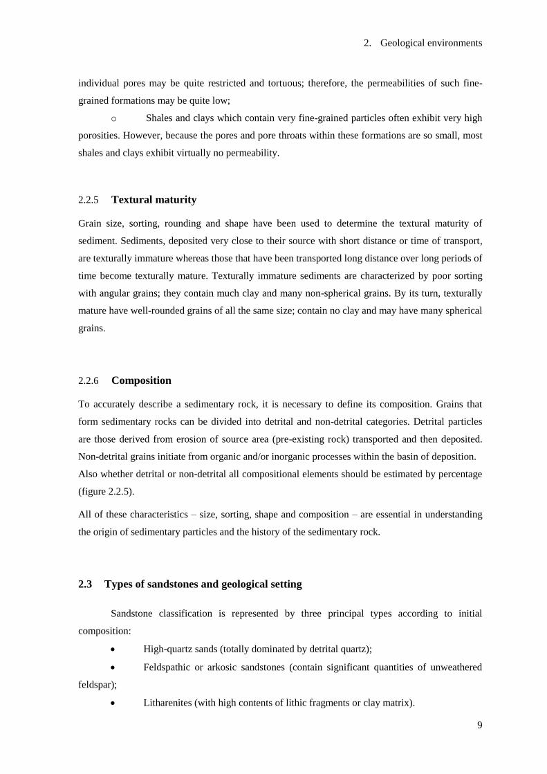
Figure 2.2.5 – Figure for estimating percentage of a component by volume (Compton, 1985).
The main interest to geologist is high-quartz sand. High-quartz sands sediments are provided by
three widespread continental terrains and geological settings:
Much thicker bodies of high-quartz sandstone comprise the molasses shed into
foreland or backarc basins from newly risen fold-trust belts (the eastern Caucasus).
In low relief cratonic interiors with sands derived from the basement or from older
sedimentary sources (Illinois Basin, the Mississippi);
In tectonically quiescent continental margins of the Atlantic type (the Niger delta);
The most part of high-quartz sands are referred to rivers.

2. Geological environments
11
2.4 Types of the rivers and their characteristics
River channels in sedimentary basins vary greatly in size. The magnitude of any channel may be
described in terms of its width and depth (height). This basic measurements help to determine the
extent of coarse-grained channel deposits. Also the mean annual discharge is very significant for
channel characterization.
As river channels possess form and magnitude it is possible to describe them (figure 2.4.1) by
combination of:
1) a planform description of channel deviation from a straight path (sinuosity, P);
2) the degree of channel subdivision by large migrating bedforms and accreting islands
around which channel reaches diverge and converge (braiding);
3) more permanent distributive channel subdivision into stationary smaller channels
(separated by floodplain) that each contain their own channel and point bar
(anastomosing).
4) Figure 2.4.1 – Sketches to show the range of river channel types (adapted after Brice,
1984).
2. Geological environments
12
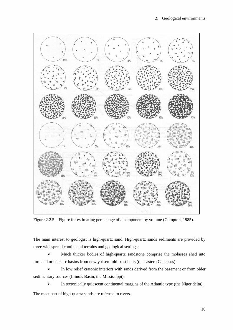
The first and the second may be expressed as numerical indices, but commonly it is more
appropriate to use qualitative terms, for instance, highly sinuous, moderately braided, etc.
According to this occurs following types of rivers (figure 2.4.2).
Figure 2.4.2 – Channel types related to the dominant type of bedload in the stream and the relative
stability of channel banks (after Orton & Reading, 1993).
2. Geological environments
13
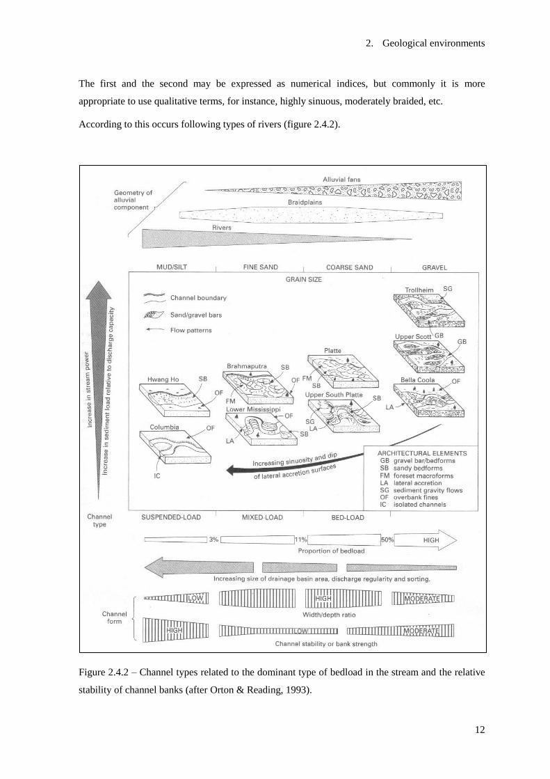
2.4.1 Braided rivers
Rivers of this type consists of several or many branching, unstable channels of low sinuosity are
characterized by abundant coarse bedload, forming bars, islands, and channel-floor deposits (figure
2.4.3a).
The channel complex typically occupies most of the valley floor, leaving little room for a
floodplain. Glacial outwash streams and ephemeral streams draining mountainous areas in arid
regions are normally braided, and may form broad sheets of sand or gravel crossed by networks of
shallow, shifting channels.
a) b)
c) d)
Figure 2.4.3 – a) Braided river, Denali National Park, Alaska (Walsh, 2007); b) meandering river,
Williams river, Alaska (Smith, 2007); c) anastamosed river, avulsion belt of the Saskatchewan
River (Smith, 2007); d) straight river, Kaa-Khem River, Siberia, Russia (Reuters, 2008).
2.4.2 Meandering rivers
These are single-channel streams of high sinuosity, in which islands and midchannel bars are rare
(figure 2.4.3b). Sediment in these rivers ranges from very coarse to very fine. A significant

2. Geological environments
14
proportion of the bedload typically is deposited on the insides of meander bends, forming point
bars. The channel, with its coarse deposits, may be confined to a narrow belt within an alluvial
valley, flanked by a broad floodplain, upon which deposition of fine-grained sediment takes place
only during flood events, seasonally or at longer intervals.
2.4.3 Anastomosed rivers
These develop in stable, low-energy environments or in areas undergoing rapid aggradation. They
consist of a network of relatively stable, low- to high-sinuosity channels bounded by well-
developed floodplains. Channels are characteristically narrow and accumulate narrow, ribbon like
sandstone bodies (figure 2.4.3c).
2.4.4 Straight channels
These are rare, occurring mainly as distributaries in some deltas (figure 2.4.3d).
Rivers which emerge from a mountainous catchment area into a low plain drop their sediment load
rapidly. The channel may bifurcate, becoming braided in character. The typical results are a
distinctive landform and an alluvial fan (see subchapter 2.9.2).
2.5 Types of river deposits
Some quantities of fluvial sands depend on the parts of the river where they are deposited. The
main parts of the river system in which significant sand bodies are deposited and preserved are the
braided section (with many channels) and the meander belt (with a single master channel on a wide
floodplain). It is possible to mark out feature appearances of deposits depending on location. For
example, a braided stream deposits are longitudinal and transverse bars of sand. In an upper low
amplitude meander belt are developed point bars on the insides of curves; in a lower meander belt –
multiple point bars. Sometimes the fluvial deposits may merge into the more widespread delta plain
deposits which include distributary channel sands.
Thereby river deposits of sediment occur as four main types:
1. Channel-floor sediments consist of the coarsest bed load, such as gravel,
waterlogged vegetation, or fragments of caved bank material;
2. Bar sediments are accumulations of gravel, sand, or silt which occur along river
banks and are deposited within channels, forming bars that may be of temporary
2. Geological environments
15
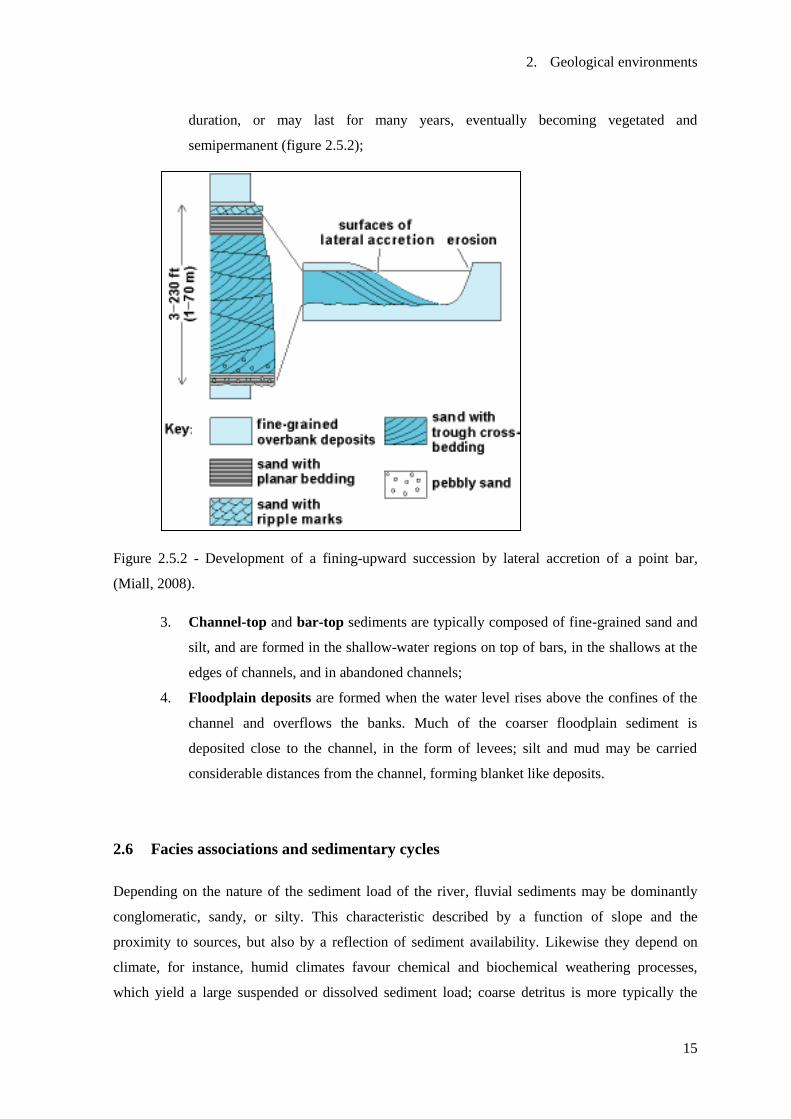
duration, or may last for many years, eventually becoming vegetated and
semipermanent (figure 2.5.2);
Figure 2.5.2 - Development of a fining-upward succession by lateral accretion of a point bar,
(Miall, 2008).
3. Channel-top and bar-top sediments are typically composed of fine-grained sand and
silt, and are formed in the shallow-water regions on top of bars, in the shallows at the
edges of channels, and in abandoned channels;
4. Floodplain deposits are formed when the water level rises above the confines of the
channel and overflows the banks. Much of the coarser floodplain sediment is
deposited close to the channel, in the form of levees; silt and mud may be carried
considerable distances from the channel, forming blanket like deposits.
2.6 Facies associations and sedimentary cycles
Depending on the nature of the sediment load of the river, fluvial sediments may be dominantly
conglomeratic, sandy, or silty. This characteristic described by a function of slope and the
proximity to sources, but also by a reflection of sediment availability. Likewise they depend on
climate, for instance, humid climates favour chemical and biochemical weathering processes,
which yield a large suspended or dissolved sediment load; coarse detritus is more typically the

2. Geological environments
16
product of drier climates, in which mechanical weathering processes (such as frost shattering) are
dominant.
It is possible to observe some vertical spatial order in the sedimentary facies described above: from
channel floor to floodplain. This order is based on decreasing grain size upward. Such deposits may
be composed by a series of fining-upward successions, or cycles, each a few meters to few tens of
meters in thickness (figure 2.6.1).
There are a variety of causes of such cycles. The first that was recognized is the mechanism of
lateral accretion, whereby point bars enlarge themselves in a horizontal direction as the meander
bounding them migrates by undercutting the bank on the outside of the bend. The depositional
surface of the point bar may be preserved as a form of large-scale, low-angle cross-bedding within
the deposit, its amplitude corresponding approximately to the depth of the channel. Similar cycles
may be caused by the nucleation and growth of large compound bars or sand flats within braided
channel systems. The accretion surfaces, in such cases, may dip in across- or down-channel
directions. Individual flood events, especially on the sand flats of ephemeral stream systems, may
form sheetlike flood cycle deposits up to a meter or so thick, the upward fining corresponding to
decreasing energy levels as the flood waned. The gradual choking of a channel with sediment, and
the progressive abandonment of the channel, will also generate a fining-upward cycle.
Figure 2.6.1 – Facies model for the Battery Point Sandstone based on analysis of vertical facies
transitions through many channel units. The model presents an ideal that is seldom complete in
nature (after Cant & Walker, 1976).

2. Geological environments
17
2.7 Tectonic Setting of Fluvial Reservoirs
The thickest and most widespread fluvial deposits accumulate in a few specific tectonic settings.
This group is divided into two main categories – extensional basins, and basins associated with
plate collision. Petroleum in fluvial mostly occurs in rift basins and foreland basins. This
localization of petroleum can be explained by specific types of tectonic setting where fluvial
deposits are volumetrically important to constitute a distinctive category of reservoir body. Such
producing units are divided into several types concerning the tectonic setting:
- Backarc foreland basins (Cano Limon oil field of Colombia);
- Backarc basins (Daqing field, China);
- Forearc basin (Cook Inlet, Alaska);
- Collision-Related Basins (Ordos Basin, China);
- Basins in Continental-Transform Setting (the South Belridge field, California);
- Rift basins (Gippsland Basin, Australia);
- Basins on External Continental Margins (The Gulf Coast of the United States);
- Intracratonic basins (Cooper Basin, Australia);
2.8 Styles of Fluvial Reservoir
The stratigraphic criteria can define three major types of nonmarine reservoirs, as shown in table
2.8 and figure 2.8.1
The primary criterion used in this classification is the type of depositional system – clastic wedge
versus incised paleovalley. The second criterion is reservoir geometry. Incised-valley fills are
ribbon bodies, clastic wedges consist of either sheet bodies or multiple lenses and ribbons enclosed
in impermeable fine-grained sediment. Last column presents most typical tectonic setting.
Table 2.8 – The three major types of petroleum reservoir in fluvial sandstones (Miall, 1996)

2. Geological environments
18
Figure 2.8.1 – Classification of nonmarine reservoirs according to the geometry of the depositional
system and the geometry of the reservoir body (Miall, 1996)
2.8.1 Paleovalley Bodies (PV Type)
Paleovalley bodies are distinguished by the ribbon or shoestring shape of the reservoir and by their
association with regional unconformities. The reservoirs typically tens of kilometers in length, up
to a few kilometers in width, and several tens of meters in thickness. The fill may be entirely
fluvial, or it may contain an estuarine component (Wood and Hopkins, 1992).
PV-type fields can occur only paleovalley fill is incised into impermeable strata, and also a top seal
and a structural component are necessary for them to generate a trap. Another type of trap is related
with the paleovalley that is folded over an anticline.
Good examples of PV-type fields are South Ceres field, Oklahoma (Lyons and Dobrin, 1972),
Recluse field, in Powder River Basin (Woncik, 1972), and Midland field, Kentucky (Reynolds and
Vincent, 1972).
2.8.2 Sheet Bodies (SH Type)
Sheet sandstones reflect high source-area relief and steep paleoslopes, with a development in most
cases of a broad braidplain. Most fields of this type require a structural trapping mechanism,
because the reservoir consists of a sheetlike porous unit providing little of fluid or not providing it
at all. Most of such type’s cases consist of large faulted anticlines in which the reservoir sandstone
is overlain by impermeable shale, for example, the Hassi Messaoud field of Algeria. Techniques of
surveillance geology (pressure tests and fluid-flow monitoring) are very powerful tools for
subsurface mapping for these type reservoirs (Miall, 1996).
2. Geological environments
19
SH-type reservoirs appear with fairly uniform internal heterogeneity within reservoir bodies at an
early exploration stage (for instance, Prudhoe Bay, Alaska), but latter they may be considered as
CB type.
2.8.3 Channel-and-Bar Bodies (CB Type)
CB-type fields are characterized by the small size of individual reservoir body, even in some cases
there may be hundreds to thousands of individual reservoirs units, can add up to significant
accumulations. Development of these fields may be extremely difficult, because they consist of the
“labyrinth” and “jigsaw” types of reservoirs (Weber and Van Genus, 1990), with tortuous flow
paths. Typical traps are entirely stratigraphic. Good examples of CB-type fields are Citronelle field,
Texas (Eaves, 1976), and Daqing field, China (Yinan et al., 1987).
Prospecting, definition of traps and development of production models for this field type, require a
detailed knowledge of depositional style. Seismic-stratigraphic mapping is important in the
delineation of small structural-stratigraphic traps, especially for basins, which are entering the
mature exploration phase, for instance, Cooper basin in Australia (Elliott, 1989).
An important aspect for production modeling may be to ascertain the degree of interconnectedness
of the reservoir units, and the definition of separate flow units within the field.
2.9 Alluvial sediments
Sometimes fluvial deposits are a part of another type – alluvial fans, extending from the subaerial
regime to the submarine. A river is continually picking up and dropping solid particles of rock and
soil from its bed throughout its length. Where the river flow is fast, more particles are picked up
than dropped. Where the river flow is slow, more particles are dropped than picked up. Areas
where more particles are dropped are called alluvial or flood plains and the dropped particles are
called alluvium.
Even small streams make alluvial deposits, but it is in the flood plains and deltas of large rivers that
large, geologically-significant alluvial deposits are found.
2.9.1 Alluvial processes
Alluvial morphologies and deposits are products of complex interactions of erosion and deposition
with the balance between them varying between different settings (Reading, 1996). Erosion occurs
at a range of physical and temporal scales. At the smallest scale, floods erode loose sediments and
2. Geological environments
20
cut small scours in cohesive fine sediment. At the large scale, floods cut new channels that range in
size from channel belts to overbank channels. Once channels are initiated, they may expand and
shift position through a combination of vertical inclination (the vertical cutting of the substrate so
that the channel deepens) and lateral migration (associated with lateral erosion). Moreover, the
transport and depositional processes that occur in alluvial channel (debris flows, bedload,
suspended load and wind) influence on sorting (for instance, fine grained, poorly sorted) and
bedforms deformations (for instance, ripples, dunes, plane beds). When sediments deposited on
alluvial fans, floodplains and in river channels they become susceptible to alteration, which cause
different physical modifications. Texture and mineralogy are modified by soil-forming processes
and early digenesis.
Thus, knowing the relationship between processes and characteristic features of the rocks it is
possible to determine the conditions under which sediments were deposited, or, studying the
conditions helps to predict the type of potential sediments.
2.9.2 Alluvial fans
Alluvial fans are a form of fluvial depositional system distinguished on the basis of geomorphic
character rather than by a characteristic fluvial style.
Alluvial fans are localized areas of enhanced sedimentation downstream of points where laterally
confined flows expand. Confinement is usually within a narrow valley or gorge cut into an area of
high relief. Flow expansion causes a reduction in depth and velocity which leads to deposition.
Alluvial fans vary enormously in scale and in terms of their active processes. Both of these reflect a
combination of source area lithology, catchment size and climate.

3. Prospection methods and interest variables
21
3. PROSPECTION METHODS AND INTEREST VARIABLES
To construct the model of reservoir is easier when parameters can be obtained by direct
measurements. Concerning the channel parameters it is extremely difficult because the reservoir is
located several thousands of meters underground and can only be described through indirect
measurements. Also they are difficult to map in detail because of frequency of lateral facies
changes and the lack of distinctiveness of individual beds in successions consisting of repeated
similar channel and overbank units (Miall, 1996). Estimating channel parameters from indirect
measurements is difficult for the following reasons:
1. Channels have irregular geometric shapes;
2. The spatial distributions of channels can only be known at very few locations (wells);
3. Permeability and porosity are spatially dependent;
4. Information is scarce;
5. Measurement techniques possess limited accuracy;
6. Data are obtained with errors;
7. The construction of mathematical models is usually not exact and complete;
8. The response of a reservoir is complex and must be computed making use of a numerical
simulator.
Nevertheless there are plenty of methods of collecting data.
3.1 The use of marker bed
The usefulness of channels deposits for mapping purpose is limited because they are not laterally
extensive. However, a few types of fluvial facies may be extensive enough to be useful for regional
mapping purpose. In addition, nonmarine environments are the ideal location for the preservation
of tephras, and these may extend for tens or hundreds of kilometres, providing ideal marker
horizons.
3.2 Wireline Logs
This technic is very old, but it is very useful for correlation purposes and helps in interpreting
fluvial style. Gamma ray logs record the presence of natural radioactivity, which typically is
highest in clay minerals (typical seals). However, the presence of clay-rich clasts in clean, coarse
sandstone may distort the reading, and feldspar-rich sandstones also yield high gamma-ray reading
3. Prospection methods and interest variables
22
(high potassium content). Thereby the most effective use of logs is in conjunction with other
lithofacies mapping techniques.
3.3 Lithofacies Mapping
These techniques as mapping of net send content, or sand/shale ratio, or net pay are standard
procedures for the delineation of reservoirs and for use in subsurface trend prediction. However,
these techniques are limited in usefulness for exploration in fluvial environments, because of the
significant facies variations, the thinness of the sandstone bodies, and their lack of directional
predictability. Narrow channels and small point bars may be missed, because in most exploration
situations well spacing is considerably bigger than the average dimensions of the typical sandstone
body. However, where well density is sufficient, detailed lithostratigraphic subdivision and channel
mapping may be rather effective.
3.4 Seismic Methods
Fluvial sandstones are commonly characterised by lenticular sandstone bodies, including
paleovalleys, cannels, and bars, but these may be difficult to detect on reflection-seismic records,
because of their small size and poor acoustic contrasts between the sandstone body and its host
strata (Miall, 1996). Sandstone channels can be identified and mapped using seismic data, but the
best results conduce to be achieved only when enough amount of local information is available, for
instance by stratigraphy reading. In other words, seismic data should not be used as the only
prospecting tool for fluvial sand bodies in frontier areas, but they may prove invaluable for
extending fields or finding infill fields in well-known areas. For instance, paleovalleys may yield
good reflections, as may a sandstone that is porous and gas filled.
The use of 3-D seismic method showed great results in detailed mapping of channels and bar
deposits in PV- and CB-type field, and even in definition of reservoir heterogeneity in SH-type
fields (figure 3.4.1).
3.5 Ground-Penetrating Radar
Ground-penetrating radar (GPR) uses radar pulses to image the subsurface; method uses
electromagnetic radiation in the microwave band (UHF/VHF frequencies) of the radio spectrum,
and detects the reflected signals from subsurface structures. Reflections occur at the interface of

3. Prospection methods and interest variables
23
beds with contrasting electrical properties, and the depth of penetration depends on the attenuation
of the signal. Greatest penetration and lowest reflectivity are yield by unconsolidated sands, gravels
and dry sandstones.
Figure 3.4.1 – Horizontal slice section, part of 3-D seismic section showing bifurcating deltaic
distributaries, Cenozoic, Gulf of Mexico (Brown, 1991).
Several applications have demonstrated the ability of the tool to map architectural details in fluvial
deposits up to 30 m in depth and 10 cm resolution. The main application of the technique is the
evaluation of sand-body architecture to study the reservoir heterogeneity.
3.6 Magnetostratigraphy
Magnetostratigraphy is used to date sedimentary and volcanic sequences. The method works by
collecting oriented samples at measured intervals throughout the section (figure 3.6.1). The
samples are analysed to determine their characteristic remanent magnetization (the polarity of
Earth's magnetic field at the time a stratum was deposited). This is possible because volcanic flows
acquire a thermoremanent magnetization and sediments acquire a depositional remanent
magnetization, both of which reflect the direction of the Earth's field at the time of formation.

3. Prospection methods and interest variables
24
Figure 3.6.1 – Magnetic sampling of fluvial succession, the Miocene-Pliocene Siwalik Group of
Pakistan. Black sample points, normal polarity, open points, reserved polarity (Behrensmeyer and
Tauxe, 1982).
Not all fluvial deposits are good for paleomagnetic study. The quality of the results decreases
hardly with increasing age, because of diagenetic complications, and reliable results depend on the
presence of fine-grained facies (because the best magnetic signature is obtained from such units) at
least every few meters from the succession.
3.7 Paleocurrent Analysis
Paleocurrent analysis is used to provide the following information:
1) Changes in channel and bar orientation and directional variability through a stratigraphic
unit (as an indicator of vertical or lateral changes in fluvial style);
2) Vertical changes in flow direction through a stratigraphic section as indicators of
interacting fluvial systems, or vertical changes in orientation of a system (as a response to
paleogeographic changes).
The use of paleocurrent data to reconstruct the details of a fluvial depositional system is a well-
established practice. Integrated basin-analysis methods couple paleocurrent data with data on facies
and grain-size trends, and perhaps information on detrital sediment composition and possible
sediment sources, the combination providing a powerful mapping technique (Miall, 1996).

3. Prospection methods and interest variables
25
3.8 The Dipmeter
The use of dipmeter as a tool for the detection and mapping of sedimentary dips promotes by
logging companies, such as Schlumberger. There are 3 main applications in the study of fluvial
sandstones:
1) The mapping of dipping fourth- and fifth-order surfaces corresponding to bar-top and
channel-floor surfaces, and the drape associated with them, providing information on the
shape and orientation of these features;
2) The mapping of internal, second- and third-order erosion surfaces (figure 3.8.1), that would
facilitate the mapping of macroforms (such as point bar);
3) The mapping of cross-bed orientations for the paleocurrent information they yield.
Figure 3.8.1 – Typical point bar and the dipping surface associated with it. The speculative
dipmeter log is also shown (Miall, 1996).
However, there are many complications for application of this technique in fluvial deposits: the
scale of cross-bedding approaches the limit of resolution at a few tens of centimetres or less and
there are many types of surface that can produce confusion (for instance, contain reactivation
surfaces).

3. Prospection methods and interest variables
26
3.9 Surveillance Geology
Surveillance geology is the monitoring of pressure and fluid composition of producing wells.
Pressure data can be used to determine the connectedness of specific sandstone bodies, and fluid
composition can be used to track the movements of oil front. Pressure-depth plots can be used to
test reservoir body connectedness (Lorenz, 1991). This information, in addition, provides data to
refine the depositional model (figure 3.9.1).
Figure 3.9.1 – Use of pressure-depth plot to test lithographic correlation. The points fall into 2
groups, indicating that they represent 2 channel-fill sandstone bodies isolated from each other by
fine-grained units. Mannville Sandstone, Alberta (Putnam and Oliver, 1980).
The pattern of the flow of oil and water depends on the porosity-permeability architecture of the
reservoir, and careful attention to the fluid movements can lead to continual refinements in the
architectural model of the reservoir.
Information on reservoir architecture and fluid movement patterns is used in production simulation
models.
3.10 Types of data and their applications
Data of different nature are collected during the life of a reservoir and can be grouped into two
classes as static and dynamic data. Static data is time-independent and has no association with fluid
transport. Geological, geophysical, petrophysical, seismic and geostatistical information are
classified as static data. Dynamic data comprise those related to the transport of fluid and are time-

3. Prospection methods and interest variables
27
dependent. This type of data could be derived from pressure transient test, shut-in surveys, down
hole permanent gauges, production history, water-cut, gas-oil ratio (GOR), and 4-D seismic
surveys.
Inverting both static and dynamic data simultaneously for reservoir characterization is a difficult
problem. A common procedure in practice is to upscale a fine-scale geological/geostatistical model
generated conditioning to static data. The upscaled model is then adjusted in such a way to quantify
dynamic data observed in the field. Current techniques for this adjustment are disconnected from
the procedure of generating the original fine-scale model. Consequently, the final reservoir model
constructed may honor the dynamic data but may not honor static data and in many cases, is
unacceptable from a geological point of view.
For reservoirs characterized by simple configurations, the model obtained by these methods
provides a good reservoir description and is sufficiently reliable for use in predicting future
reservoir performance. However, other cases, particularly in many fluvial systems, often require a
more reliable model - the model that honors the most available information. The introduction of
dynamic data (time-dependent data) in the problem of characterization of fluvial reservoirs is
useful in terms of obtaining detailed model configurations and significantly reducing the
uncertainty in modeling and in reservoir predictions.
4. Methodology and theoretical background
28
4. METHODOLOGY AND THEORETICAL BACKGROUND
Fluvial reservoirs offer a particular challenge for modelling (Matheron et al, 1987; Luis and
Almeida, 1997) due to their variable geometries and complex networks. In particular fluvial sands
reservoirs are characterized by their elongate shapes with a relatively small width-length ratio.
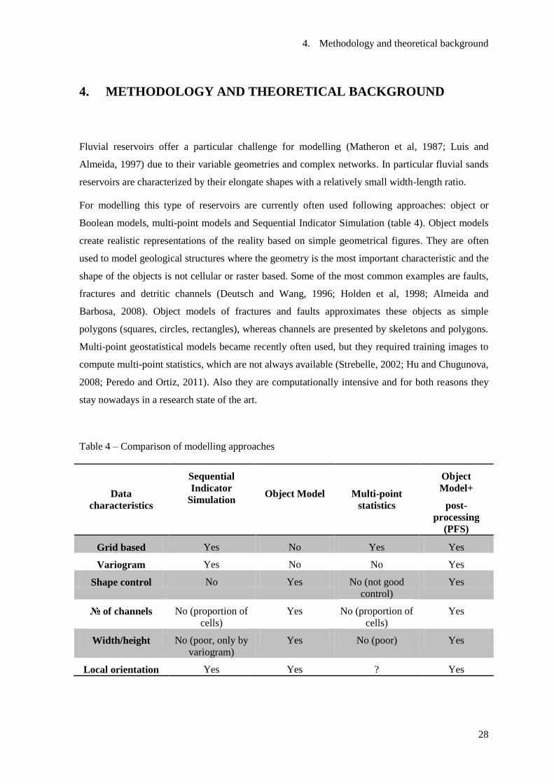
For modelling this type of reservoirs are currently often used following approaches: object or
Boolean models, multi-point models and Sequential Indicator Simulation (table 4). Object models
create realistic representations of the reality based on simple geometrical figures. They are often
used to model geological structures where the geometry is the most important characteristic and the
shape of the objects is not cellular or raster based. Some of the most common examples are faults,
fractures and detritic channels (Deutsch and Wang, 1996; Holden et al, 1998; Almeida and
Barbosa, 2008). Object models of fractures and faults approximates these objects as simple
polygons (squares, circles, rectangles), whereas channels are presented by skeletons and polygons.
Multi-point geostatistical models became recently often used, but they required training images to
compute multi-point statistics, which are not always available (Strebelle, 2002; Hu and Chugunova,
2008; Peredo and Ortiz, 2011). Also they are computationally intensive and for both reasons they
stay nowadays in a research state of the art.
Table 4 – Comparison of modelling approaches
Data
characteristics
Sequential
Indicator
Simulation
Object Model
Multi-point
statistics
Object
Model+
post-
processing
(PFS)
Grid based Yes No Yes Yes
Variogram Yes No No Yes
Shape control No Yes No (not good
control)
Yes
№ of channels No (proportion of
cells)
Yes No (proportion of
cells)
Yes
Width/height No (poor, only by
variogram)
Yes No (poor) Yes
Local orientation Yes Yes ? Yes

4. Methodology and theoretical background
29
Objects can be simulated in space based on local or regional characteristics, such as density,
orientation, size, etc. Therefore, most of the times objects are generated or simulated in space
conditioned to stochastic measurements and characteristics extracted from well or seismic data.
Simulation of channels in 3D space is adequate for object modelling procedures, as channels
follows a complex geometry and the shape behaviour cannot be fully characterized only by two-
point statistics. However, an object model of channels, even if conditioned to experimental
statistics of shape and density, is not realistic and must be post-processed.
To generate realistic 3D morphological models for fluvial sand channels reservoirs, the idea of the
proposed methodology is to combine object and geostatistical simulation models to generate a set
of equally probable scenarios. Those scenarios can be filled with petrophysical properties in a
second step.

4. Methodology and theoretical background
30
4.1 Methodology
The workflow of the proposed methodology is represented in the figure 4.1 and is detailed next.
Figure 4.1 – Workflow of the proposed methodology.
1
5 5
6 7
3 4
Local orientations image
Channels height (m)
Channels width (m)
2
Input: seismic data, well data, geological knowledge
1. Prepare morphological sizes statistics (length, width, height) and local orientations (azimuth and dips)
2. Geostatistical simulation of the width and height of the channels
3. Build of a Boolean model of the channels (vector type model)
4. Conversion from vector to raster and assign regions of uncertainty
5. Use of PFS algorithm (probability field simulation) to post-process the
Boolean model according a variogram
6. Simulation of properties within the channels (SSG or DSS)
7. Reservoir and potential OIP evaluation

4. Methodology and theoretical background
31
Step 1: Data preparation. Input data for this flowchart consists of channels measurements (length,
width and height), channels density and local channels orientation. Sizes can be considered by
synthesis statistics (mean and variance under a distribution law) or for instance by cumulative
histograms. A coefficient of correlation between channel width and height sizes can also be used.
Channels density can be expressed as a fraction of channels volume by region, level or whatever.
Local channels orientations are local azimuths and dips angles of the channels skeleton (See
example for azimuths in figure 4.2). All those starting data can be obtained by geology expertize,
similar geological formations, seismic interpretation together with well data (cores and logs) if
available.
The relationship between channels measurements and channels density conditions the number of
channels to be simulated within a specific volume. Local channels orientation conditions the
sinuosity of the channels and the reciprocate connectivity. If local orientations are provided only at
some locations, it is prior necessary to interpolate (for instance by kriging) both angles (azimuth
and dip) into a 2D or 3D grid according the reservoir grid block model.
Figure 4.2 – Example of an image of local orientations (azimuths).
Step 2 Geostatistical simulation of the width and height of the channels. The objective of this
step is to provide a pseudo-continuous value for the width and height of each channel to be
simulated, conditioned to the histograms of width and height mentioned in the previous step. In the
present work, it is proposed to simulate those values with Sequential Gaussian Simulation (SGS) or
Direct Sequential Simulation within a synthetic 2D grid. Each column of this grid represents a
hypothetical channel to be simulated and the rows represent the channel discretization in
accordance with the reservoir grid block model. Thus, this 2D grid should be initiated with the
number of columns equal to the maximum number of channels to be simulated and the number of
rows equal to the maximum length of the channel divided by the reservoir grid block size.
22 25 58 83 90
18 28 62 85 90
12 30 75 85 90
9 30 75 85 90
7 25 60 90 97
N
Az
angle

4. Methodology and theoretical background
32
For simulation, variogram between columns should be a pure nugget effect (no relationship
between channels size) and between rows a range and a theoretical function must be considered. A
relationship between widths and heights can be imposed if simulation of heights (or widths) are
constrained to each other, for instance, using a co-simulation procedure (Co-DSS).
Step 3: Build of a Boolean model of channels. In this step, an object or Boolean model of the
channels is generated following a vector structure of the data. In section, channels can be modelled
by simple figures such as rectangles, half circles (width equal to height) or half ellipsoidal shapes,
which was the approximation adopted in the present case study. Generation / simulation is
performed channel by channel: a) generate a maximum length for the channel by Monte Carlo
simulation from lengths histogram; b) random generation of an initial point location of the channel;
c) from the initial point, grow skeleton of the channel for both sides, according local orientation
angles plus a tolerance, and until channel reaches the predefined maximum length or the
boundaries of the reservoir (see figure 4.3 left); d) select a trace of widths and heights simulated in
the previous step and evaluate the volume of the channel assuming a U shape (see figure 4.3 right);
e) simulate new channels using the same procedure until a previously defined objective in terms of
channels proportion is reached. Output of this step is a set of arcs each of them represents the
skeleton of a channel.
Figure 4.3 – Generation of a 3D channel: (left) simulation of the skeleton; (right) assign local
widths and heights.
1
2
3 4 5
6
7
8
1
2
Generation of the next point of the channel according local orientations and a tolerance
Channel section
4. Methodology and theoretical background
33
If well data is available, the simulation of the skeleton of the channels should begin from the well
location, and in this case the exact location of the channel can be ajusted acording the height
measure at the well and the height obtained by simulation. From this initial point, channels should
increase from both sides until the objective-simulated length is achived. In these cases the post
processing PFS keeps blocks classified as channels acording the well data.
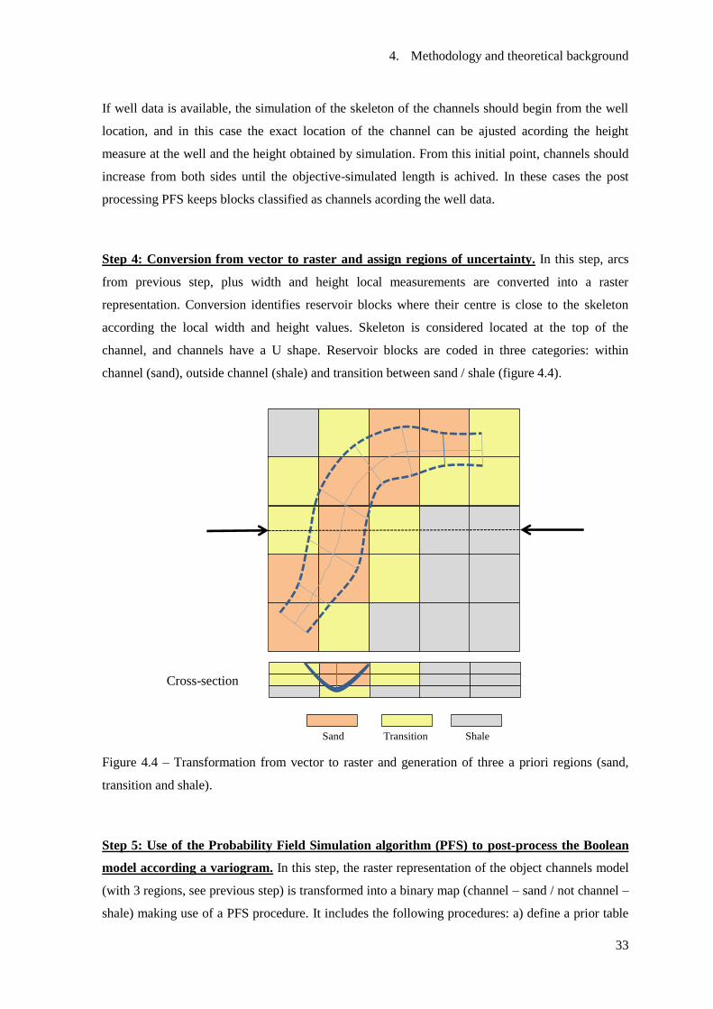
Step 4: Conversion from vector to raster and assign regions of uncertainty. In this step, arcs
from previous step, plus width and height local measurements are converted into a raster
representation. Conversion identifies reservoir blocks where their centre is close to the skeleton
according the local width and height values. Skeleton is considered located at the top of the
channel, and channels have a U shape. Reservoir blocks are coded in three categories: within
channel (sand), outside channel (shale) and transition between sand / shale (figure 4.4).
Figure 4.4 – Transformation from vector to raster and generation of three a priori regions (sand,
transition and shale).
Step 5: Use of the Probability Field Simulation algorithm (PFS) to post-process the Boolean
model according a variogram. In this step, the raster representation of the object channels model
(with 3 regions, see previous step) is transformed into a binary map (channel – sand / not channel –
shale) making use of a PFS procedure. It includes the following procedures: a) define a prior table
Cross-section
Sand Transition Shale

4. Methodology and theoretical background
34
for transformation of values, meaning the probability of each a priori region became a channel
(sand facies); b) simulate an image of Gaussian values conditioned to a variogram model and the
local orientations of the grid; c) transform the Gaussian map into a probability map; d) apply the
PFS and get final images of the sand / shale geometry.
Step 6: Simulation of properties within channels. Making use of the previous simulated images
of channels, it is possible to generate properties within and outside the channels, such as porosity
and permeability, if well data and histograms are available. In the present thesis, and only for
demonstrative purposes, porosity values are generated by Direct Sequential Simulation (DSS) with
regional histograms.
Step 7: Reservoir and potential OIP evaluation. In this final step, and also for demonstration
purposes, curves of potential Oil in Place (OIP) calculated with porosity grids are presented.
4.2 Background of geostatistics
Geostatistics is a branch of statistics dealing with the problems associated with space (and / or
time), and aims to characterize the spatial distribution (and / or temporal) of measured and present
their local and global uncertainty, taking into regard a density, zoning and heterogeneity of the
available information (Soares, 2006).
The geostatistics background was first proposed by Matheron, in sixties of the last century, with the
characterization of mineral deposits. Later, geostatistics were extended for the characterization of
oil reservoirs, natural resources and environmental problems, since all these phenomena are
characterized by variables which are governed by the same statistical principles.
In summary, the use of geostatistical methodologies involves the three issues:
a) Data analysis;
b) Spatial analysis (calculation and fitting of experimental variograms);
c) Forecast (kriging estimation and/or simulation).
The basic paradigm of geostatistics is to convert the hypothetical value of each location not
sampled in a realization of a random variable , whose distribution law allows us to understand
and model the spatial variability.
4. Methodology and theoretical background
35
A random variable ( ) is a variable that can assume a set of values ( ) according a distribution law.
The random variable ( ), or more specifically the distribution law, is dependent of the location, and
that’s why it is usual to present associated to a location . The random variable is also
dependent of the known information, which means, the distribution law changes when the
information of the not sampled location increases.
Random variables can be categorical or continuous. Lithology, facies and colours are examples of
categorical variables; petrophysical properties (porosity, permeability and density), grades and
geographical properties (elevation, thickness and depths) are examples of continuous variables.
The cumulative distribution function (cdf) of a continuous random variable , can be expressed
by:
{ }
When the cdf is presented for a location , taking into account a set of neighbour samples of
location , it is used the designation “conditional to”:
{ }
In geostatistics, most of the information related with an unsampled location is given by the
neighbour samples of the same attribute or another if correlated. Thus, it is important to
model the correlation or dependence between the random variables
and .
A random function is a set of random variables defined for the same area in study {
}.
As a random variable is characterized by their cdf, a random function is characterized by the set of
K- cdf given for locations, .
{ }
As a univariate cdf of the random variable is used to characterize the uncertainty of z , the
multivariate cdf is used to characterize the joint uncertainty of the values .
The geostatistical methods presuppose that the random variables present simultaneously:
• A random pattern, which means, for small distances random variations exists;
• A structured pattern and, therefore, predictable (geology, grades dispersion).

4. Methodology and theoretical background
36
The random component may be more or less predominant, associated with the variability of the
phenomenon and their sampling, such as errors due to data collection, or the existence of different
procedures for the quantification of the same attribute.
The geostatistics assumes that the statistical distribution of the difference of values of a variable
between pairs of points (samples) is similar in all study area and depends only on the distance and
orientation of pairs of points. This assumption is a designation of stationarity (2nd
order), and is the
fundamental concept assumed in geostatistics. In summary, classic statistic does not take into
account the location of the samples, and the geostatistic uses the location of each sample in relation
with the neighbour samples.
This leads to the concept of a regionalised variable, which is a variable defined at a specific
location of the study area that depends of the magnitude and the sample size (volume, shape and
orientation). Typical examples of regionalised variables that can be worked with geostatistics are,
for example, the thickness of a mineralized body, the bulk density, and physical parameters of the
rock porosity, etc.
Given the impossibility of fully evaluate, in space and / or time, the distribution of the property in
study, the characterization is usually based on a limited set of data obtained by several samples.
The data collection presents specific characteristics associated with a certain degree of uncertainty
and unique achievements making it impossible to repeat the observation in a given space and time.
Validation of the geostatistical models used in the characterization of the resources it will need to
be made a posteriori by the intersection between the results obtained through modeling and the
available data, which determines a greater or lesser distance (error) to reality.
In geostatistics are considered two evaluation strategies: estimation and simulation (Deutsch and
Journel, 1992; Goovaerts, 1997; Soares, 2006). The estimation models or geostatistical
interpolation are based on the formalism of kriging and aim to obtain an average picture of the
phenomenon (variable) in the study. There are several variants of kriging (ordinary, simple) or
kriging that consider the indirect information (cokriging, collocated cokriging, kriging with an
external drift), or that are applied to categorical variables (indicator kriging) or continuous.
In estimation, we want to make the best possible estimate at the unsampled location via kriging, by
minimalizing the error variance. However, there is no guarantee that the map obtained using
kriging has the same variogram and variance as the original data.
The simulation models are to obtain a set of images as a whole that equiprobable quantifies of a
local and global uncertainty. It allows us to come up with theoretically an infinite number of
realizations of the map each of which has approximately the same variogram and variance of the
original data.
4. Methodology and theoretical background
37
One important use of simulation is in the petroleum industry. Simulated images allow petroleum
engineers to have a range of fluid flow predictions all of which are plausible given the uncertainty
in the distribution of the geological properties.
4.3 Spatial continuity and variograms
4.3.1 Variogram and spatial continuity
The dependence between observations can be evaluated with the variogram tool, which is a spatial
correlation measurement by reference to a vector . The experimental variogram is calculated
by the half-sum of the squares of differences between pairs of measurements in the direction of the
vector and separated by , where is the number of pairs of points separated by a vector .
( )
∑[ ]
For a specific direction, or set of directions, the values of are usually represented graphically
with the distance (module of vector ). The increment of , with the distance, depends of the
gradient of a sample value changes related with the distance. When stabilizes the maximum
correlation distance is reached.
Another measurement of spatial continuity is the spatial covariance which can be calculated by:
( )
( )∑ ( )
( )
Where
∑
and
∑
are the left and right averages
regarding vector , respectively.
The spatial covariance is related with the variogram by ( ) where
| | is the statistical variance of the data.
4.3.2 Fitting of theoretical models
The experimental variograms obtained for different directions, from the information available,
allow analysis of the structure of continuity of the variable under study. These experimental

4. Methodology and theoretical background
38
variogram estimators can be interpreted as a comprehensive theoretical model, calculated only for
some ranges of distance and directions. For this reason, the experimental variogram must be fitted
by a theoretical function satisfying the requirement of being positive definite.
The theoretical model can be defined by a unique function, or a sum of theoretical functions as the
sum of two positive-defined functions is still a function defined positive. The final model can be
isotropic or not, as it is constant or not, according to the various directions.
The most common theoretical function is designated by spherical or Matheron. The growing
behaviour of this function is more pronounced for shorter distances and then more slowly to reach a
plateau (sill).
{
[
(
)
]
Where C is the sill (variance of the data), is the range or maximum correlation distance and h is
the distance.
Another widely used function is the exponential model.
(
) [ (
)]
For all models it is also possible to add a nugget effect ( ). The nugget effect can be interpreted as
an indicator of the variability of the studied variable under the sampling distance.
Graphically, the nugget effect is represented as the ordinate at the origin of the graph representation
of the semi-variogram versus distance. Theoretically can range between 0 (no nugget effect) and
the sill of the variogram (pure nugget effect).
4.4 Simulation strategies
The models used in geostatistical modelling of phenomena are related to quantification of
categorical and continuous variables describing natural resources that are possessed of a spatial
structure, resulting from the association of behaviour with the theoretical foundations of
mathematics and statistics, in particular the theory of random functions.

4. Methodology and theoretical background
39
The choice of a particular geostatistical model should be based on the study and knowledge of the
natural phenomenon in question, incorporating its spatial component in their characterization,
which can be used for different applications in the areas of planning, recovery and monitoring the
natural or more specifically geological resource. Validation of the geostatistical models is made a
posteriori by the intersection between the results obtained by modeling and the available real data,
which allows you to find a greater or lesser distance to the reality (space of uncertainty).
Geostatistical simulation is a stochastic process for generating images that reproduce the spatial
distribution and uncertainty associated with different variables addressed in the Earth Sciences.
This class of models aims to reproduce images of reality that reflect characteristics of the resource,
such as the variability of the sample set, the distribution law of the variable under study, and spatial
continuity. The result is a set of equiprobable images with the same spatial distribution of the
experimental data, and reproduction of statistical and spatial variability quantified by the samples
(histogram and variogram or spatial covariance). Typically, the simulation is not intended to obtain
the average or the most likely characteristics of a given variable / resource (which is the objective
of estimation), but a set of equiprobable images, enabling different views of a resource, and
simultaneously quantify the uncertainty of these site characteristics given by the available data.
There are several simulation algorithms to generate images, but in this study sequential simulation
and probability field simulation were used and therefore are described shortly below.
4.4.1 Sequential simulation methods
With a simulation model it is intended to reproduce in the simulated image, the variability of the
phenomenon under study by two statistical measurements { } –
frequency of the classes histogram and the variogram that reproduces the spatial continuity of
.
If designates the simulated dataset, and , , the experimental values, the
simulated images must fulfil the following itens:
1. For any value of { } { }.
2. , where and are respectively the variograms of the experimental
and simulated values.
3. At any experimental location the know value and the simulated value
matches: . The simulated image has the same variability as the original
data and matches the experimental known values.
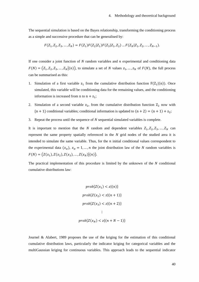
4. Methodology and theoretical background
40
The sequential simulation is based on the Bayes relationship, transforming the conditioning process
as a simple and successive procedure that can be generalised by:
If one consider a joint function of random variables and experimental and conditioning data
( | ), to simulate a set of values of , the full process
can be summarised as this:
1. Simulation of a first variable from the cumulative distribution function . Once
simulated, this variable will be conditioning data for the remaining values, and the conditioning
information is increased from to ;
2. Simulation of a second variable , from the cumulative distribution function now with
{ } conditional variables; conditional information is updated to
3. Repeat the process until the sequence of sequential simulated variables is complete.
It is important to mention that the random and dependent variables can
represent the same property spatially referenced in the grid nodes of the studied area it is
intended to simulate the same variable. Thus, for the initial conditional values correspondent to
the experimental data , the joint distribution law of the random variables is
( | )
The practical implementation of this procedure is limited by the unknown of the conditional
cumulative distributions law:
{ }
{ }
{ }
{ }
Journel & Alabert, 1989 proposes the use of the kriging for the estimation of this conditional
cumulative distribution laws, particularly the indicator kriging for categorical variables and the
multiGaussian kriging for continuous variables. This approach leads to the sequential indicator

4. Methodology and theoretical background
41
simulation (SIS) and sequential Gaussian simulation (SSG), for categorical and continuous
variables, respectively (Nunes and Almeida, 2010).
As the sequence of the simulation of the nodes is random, as well as the generation of the
simulated value at each node using a Monte Carlo procedure, each realization is independent. All
simulated images are equally probable, match the histogram, variogram and the original data at
samples locations.
4.4.2 Sequential Gaussian simulation
The sequential Gaussian simulation (SGS) is a procedure where all values of the variable under
study are prior transformed to a Gaussian distribution law, [ ], and all process is
developed within a Gaussian framework (Journel, 1989). Back transform of the simulated Gaussian
values for the original distribution law is performed at the end. It is a parametric approach in the
sense that kriging estimates the local mean and variance of a Gaussian distribution type.
4.4.3 Direct Sequential simulation
For continuous variables, the Direct Sequential simulation (DSS), unlike SGS, uses the original
variable without any previous transformation of the data. For instance, as SGS uses a prior
transformation of the data to a Gaussian distribution, and a back-transformation at the end, it is
sometimes difficult to reproduce the variograms of the original variable mainly for extremely skew
distributions. This effect increases if secondary variables are used within a co-simulation
procedure.
The DSS as proposed by Soares, 2001, uses the local mean and variance to resample the global
cumulative distribution law , and build a new local cumulative distribution function
with intervals centred on the local estimated average and with a range proportional to the local
conditional variance. Those two local parameters mean and variance are estimated by simple
kriging:
[ ] ∑
One way to define the intervals and get the simulated value from is to select a subset
of contiguous values of the global experimental histogram whose mean and variance of the
selected values is equal to the local estimated mean [ ] and estimation variance
:
4. Methodology and theoretical background
42
∑[ [ ]
]
∑ [ ]
Another way to define the function is to use a Gaussian distribution law only as a helper function to
re-sample intervals and not to transform the original data to Gaussian distribution.
The following sequence of steps summarizes the simulation of a variable via SSD:
1. Define a random path visiting each node of a regular grid of nodes.
2. At , node to be simulated, kriging estimation of the local mean and variance
conditional to the experimental data and the nodes previously simulated.
3. Definition of the intervals for resampling of the global distribution law , by a
Gaussian transformation [ ] , where [ ]
[ ] , being the
normal score transform of the variable.
4. Calculation of the simulated value :
a. Generate a value from an uniform distribution
b. Generate through (
)
c. Return of the simulated value .
5. Repeat steps 2-5 until all nodes are simulated.
To highlight the contract between properties within and outside the channels, and to avoid to run
two simulations of properties, for the simulation of the porosity conditioned to the facies presented
in the last part of the case study, the histograms used for resampling are not the global histogram
but two local histograms, one for channel data and another for not channel data (Roxo, 2011).
4.4.4 Probability field simulation
Once allocated a priori probability of each grid node belonging to a channel (output object based
model) via regions or classes (cl) of uncertainty (ncl=3 in the present case study) (cl=1 high
probability of being a channel; cl=2 50% of being a channel and cl=3 low probability of being a
channel), the Probability Field Simulation (PFS) step of the proposed methodology (Srivastava,
1992, Froidevaux, 1993) has the objective of reclassify the a priori probabilities into a binary image
(channel / not channel). This procedure transforms the object-based model (smooth shapes) into a
more realistic model imposing a theoretical model of variogram.

4. Methodology and theoretical background
43
In particular, for each location the cumulative distribution function corresponding to the class cl
allocated to is known:
{ }
If a probability field image is generated for the entire area thus the simulated
value is equal to:
where )
The probability field image can be generated by simple transformation of a Gaussian image
provided by a geostatistical simulation algorithm for continuous variables, such as SGS or the
turning band method.
In this particular case study, the probability field map is generated regarding local orientations of
the covariance (Soares, 1990) (figure 4.5).
Figure 4.1 – (top left) Simulated image of gaussian values conditioned to local ellipsoid
orientations ; (top right) Homologous probability field simulated image; (bottom) local ellipsoid
orientations (only for illustrative purposes, no correspondence with the top images).

4. Methodology and theoretical background
44
To apply local orientations, the covariances of the right matrix of the kriging system are rotated of
degrees, which is the angle of the main direction of the ellipsoid of anisotropy in the location to
estimate / simulate.

5. Case study
45
5. CASE STUDY
A stochastic methodology for modelling fluvial reservoirs composed of discontinuous sands is
presented in previous section. A synthetic case study for demonstrative purposes is presented in
this section.
5.1 Starting data
Reliable statistical starting data is a pre-requisite of successful probabilistic modelling of fluvial
reservoirs. Starting data for the proposed morphology consists of:
a) Histogram of lengths;
b) Histogram of widths and heights and a ratio or a correlation coefficient width-height;
c) Images of the local orientation angles (azimuths, 2D and dips, 3D).
In real case studies, this information should be provided by geological expertise, seismic or other
sources.
For modelling purposes, it was initiated a synthetic grid of blocks with the characteristics listed in
table 5.1.
Table 5.1 – Parameters of the synthetic reservoir grid blocks.
X direction Y direction Z direction
Number of blocks 200 200 30
Block sizes (m) 30 30 2
Initial coordinates 0 0 0
Concerning lengths, widths and heights (dimensions of the channels), three cumulative histograms
were initiated (figure 5.1). Lengths range between 300m (10 grid blocks) and 6000m (maximum
size of the studied area); widths range between 110m (3-4 grid blocks) and 285m (approximately
minimum length of the channels); and finally heights range between 2 (one reservoir block) and 8
meters (4 reservoir blocks). A relationship between width and height dimensions via a correlation
coefficient was used.

5. Case study
46
Figure 5.1 – Cumulative histograms of the length, width and height dimensions.
For this study, an image of the local directions of flow (angles relative to the North) was also
constructed. This image was built on ArcGIS from a digital terrain model where hydrological
functions such as FILLMDT and FlowDirection were applied (figure 5.2).
Figure 5.2 – Flow direction angles or local orientation of the potential flow (Aljustrel, Alentejo).
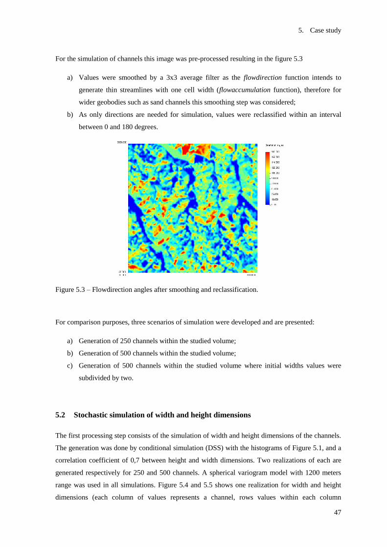
5. Case study
47
For the simulation of channels this image was pre-processed resulting in the figure 5.3
a) Values were smoothed by a 3x3 average filter as the flowdirection function intends to
generate thin streamlines with one cell width (flowaccumulation function), therefore for
wider geobodies such as sand channels this smoothing step was considered;
b) As only directions are needed for simulation, values were reclassified within an interval
between 0 and 180 degrees.
Figure 5.3 – Flowdirection angles after smoothing and reclassification.
For comparison purposes, three scenarios of simulation were developed and are presented:
a) Generation of 250 channels within the studied volume;
b) Generation of 500 channels within the studied volume;
c) Generation of 500 channels within the studied volume where initial widths values were
subdivided by two.
5.2 Stochastic simulation of width and height dimensions
The first processing step consists of the simulation of width and height dimensions of the channels.
The generation was done by conditional simulation (DSS) with the histograms of Figure 5.1, and a
correlation coefficient of 0,7 between height and width dimensions. Two realizations of each are
generated respectively for 250 and 500 channels. A spherical variogram model with 1200 meters
range was used in all simulations. Figure 5.4 and 5.5 shows one realization for width and height
dimensions (each column of values represents a channel, rows values within each column
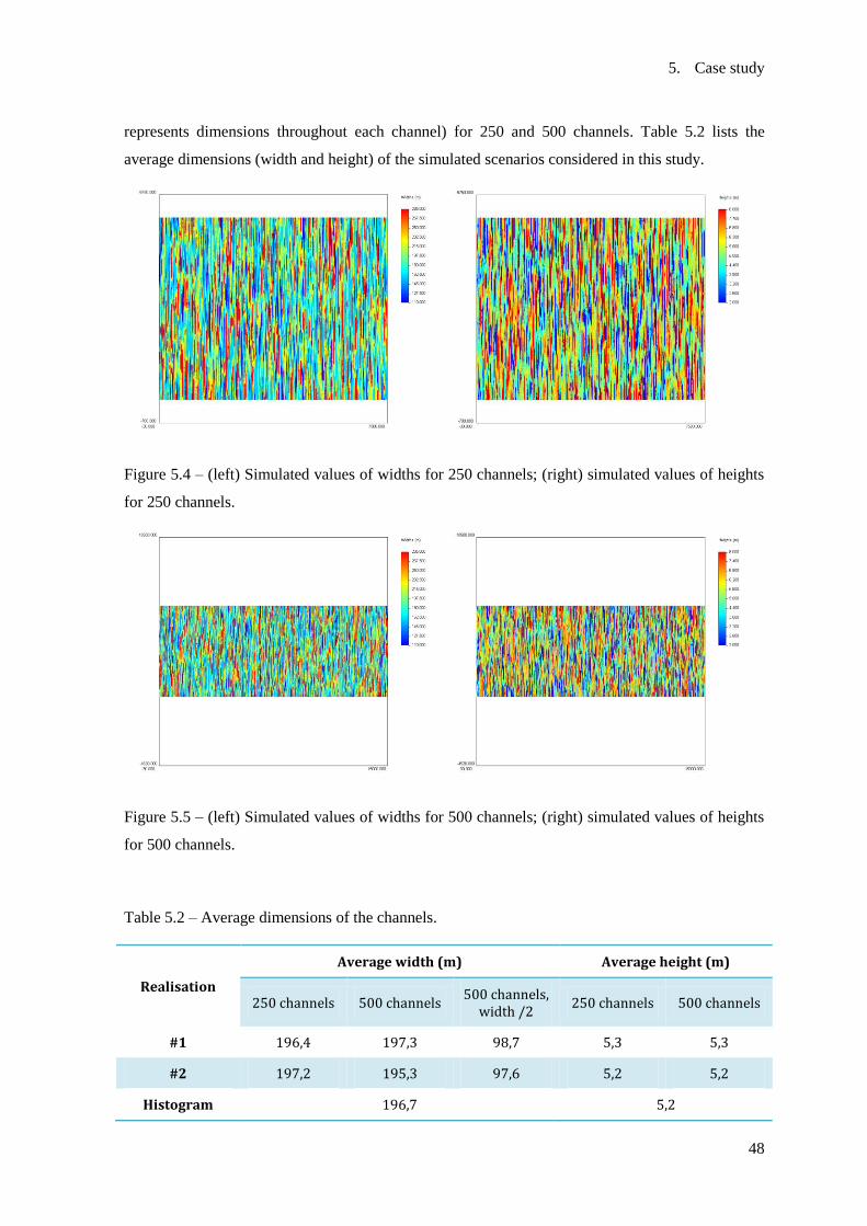
5. Case study
48
represents dimensions throughout each channel) for 250 and 500 channels. Table 5.2 lists the
average dimensions (width and height) of the simulated scenarios considered in this study.
Figure 5.4 – (left) Simulated values of widths for 250 channels; (right) simulated values of heights
for 250 channels.
Figure 5.5 – (left) Simulated values of widths for 500 channels; (right) simulated values of heights
for 500 channels.
Table 5.2 – Average dimensions of the channels.
Realisation
Average width (m) Average height (m)
250 channels 500 channels 500 channels,
width /2 250 channels 500 channels
#1 196,4 197,3 98,7 5,3 5,3
#2 197,2 195,3 97,6 5,2 5,2
Histogram 196,7 5,2
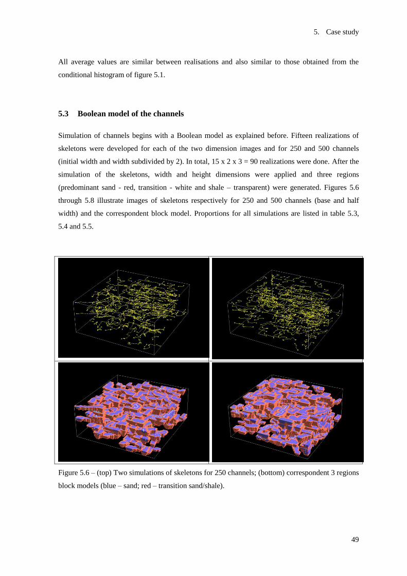
5. Case study
49
All average values are similar between realisations and also similar to those obtained from the
conditional histogram of figure 5.1.
5.3 Boolean model of the channels
Simulation of channels begins with a Boolean model as explained before. Fifteen realizations of
skeletons were developed for each of the two dimension images and for 250 and 500 channels
(initial width and width subdivided by 2). In total, 15 x 2 x 3 = 90 realizations were done. After the
simulation of the skeletons, width and height dimensions were applied and three regions
(predominant sand - red, transition - white and shale – transparent) were generated. Figures 5.6
through 5.8 illustrate images of skeletons respectively for 250 and 500 channels (base and half
width) and the correspondent block model. Proportions for all simulations are listed in table 5.3,
5.4 and 5.5.
Figure 5.6 – (top) Two simulations of skeletons for 250 channels; (bottom) correspondent 3 regions
block models (blue – sand; red – transition sand/shale).
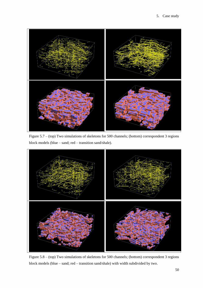
5. Case study
50
Figure 5.7 – (top) Two simulations of skeletons for 500 channels; (bottom) correspondent 3 regions
block models (blue – sand; red – transition sand/shale).
Figure 5.8 – (top) Two simulations of skeletons for 500 channels; (bottom) correspondent 3 regions
block models (blue – sand; red – transition sand/shale) with width subdivided by two.

5. Case study
51
Table 5.3 – Proportions of the different regions (shale, sand, and transition shale-sand) by
realization, scenario of 250 channels.
250 channels, realization #1 of width-height 250 channels, realization #2 of width-height
Shale Shale-Sand Sand Shale Shale-Sand Sand
1 0.758 0.112 0.130 0.739 0.123 0.138
2 0.726 0.128 0.146 0.742 0.121 0.137
3 0.749 0.118 0.134 0.757 0.115 0.128
4 0.745 0.120 0.135 0.759 0.115 0.127
5 0.743 0.121 0.136 0.755 0.114 0.132
6 0.744 0.120 0.135 0.756 0.114 0.130
7 0.749 0.119 0.132 0.740 0.120 0.140
8 0.744 0.119 0.137 0.729 0.126 0.145
9 0.749 0.118 0.133 0.757 0.112 0.131
10 0.753 0.116 0.131 0.748 0.116 0.136
11 0.760 0.112 0.128 0.749 0.118 0.133
12 0.742 0.120 0.138 0.744 0.120 0.136
13 0.756 0.112 0.132 0.751 0.118 0.130
14 0.736 0.124 0.141 0.752 0.116 0.132
15 0.745 0.120 0.135 0.754 0.115 0.131
Average 0.747 0.119 0.135 0.749 0.118 0.134
Table 5.4 – Proportions of the different regions (shale, sand, and transition shale-sand) by
realization, scenario of 500 channels.
500 channels, realization #1 of width-height 500 channels, realization #2 of width-height
Shale Shale-Sand Sand Shale Shale-Sand Sand
1 0.578 0.216 0.206 0.572 0.216 0.212
2 0.563 0.220 0.217 0.573 0.217 0.210
3 0.577 0.210 0.214 0.579 0.213 0.208
4 0.565 0.221 0.214 0.571 0.220 0.209
5 0.573 0.214 0.213 0.566 0.217 0.217
6 0.576 0.212 0.212 0.566 0.218 0.216
7 0.575 0.214 0.211 0.586 0.209 0.205
8 0.556 0.227 0.218 0.564 0.220 0.216
9 0.568 0.216 0.215 0.573 0.217 0.211
10 0.590 0.206 0.204 0.583 0.210 0.207
11 0.578 0.213 0.209 0.569 0.218 0.213
12 0.573 0.216 0.211 0.566 0.219 0.215
13 0.591 0.209 0.199 0.575 0.216 0.209
14 0.581 0.213 0.206 0.582 0.214 0.204
15 0.578 0.216 0.206 0.582 0.209 0.209
Average 0.575 0.215 0.210 0.574 0.216 0.211

5. Case study
52
Table 5.5 – Proportions of the different regions (shale, sand, and transition shale-sand) by
realization, scenario of 500 channels, width / 2.
500 channels, realization #1 of width-height 500 channels, realization #2 of width-height
Shale Shale-Sand Sand Shale Shale-Sand Sand
1 0.846 0.087 0.067 0.846 0.087 0.067
2 0.846 0.089 0.066 0.852 0.084 0.064
3 0.843 0.089 0.068 0.849 0.085 0.066
4 0.845 0.087 0.068 0.840 0.091 0.070
5 0.839 0.091 0.070 0.847 0.087 0.067
6 0.845 0.088 0.067 0.851 0.084 0.065
7 0.841 0.089 0.069 0.840 0.090 0.070
8 0.850 0.085 0.065 0.840 0.090 0.070
9 0.842 0.088 0.069 0.846 0.087 0.067
10 0.848 0.086 0.066 0.842 0.089 0.068
11 0.850 0.085 0.065 0.847 0.086 0.067
12 0.846 0.087 0.067 0.845 0.087 0.068
13 0.840 0.091 0.070 0.840 0.091 0.070
14 0.849 0.085 0.066 0.847 0.086 0.067
15 0.838 0.093 0.070 0.844 0.088 0.068
Average 0.845 0.088 0.068 0.845 0.087 0.068
5.4 Probability Field Simulation
Probability field simulation (PFS) algorithm was used for this next step of the methodology to post-
process the object model and transform the transition zone conditioned to a variogram model. PFS
begins with the simulation of a probability image with a uniform distribution law between 0 and 1.
Sixty simulated images were generated and the first two are represented in figure 5.9. For
demonstration purposes, theoretical model of variogram was defined in accordance with the
dimensions previous proposed for channels: spherical model with 3000 meters in main direction,
200 m in the perpendicular at horizontal and 10m in vertical. As can be seen in the figure,
probability maps follows the local orientations defined before.
Figure 5.9 – Examples of two simulated probability images used for PFS purposes.
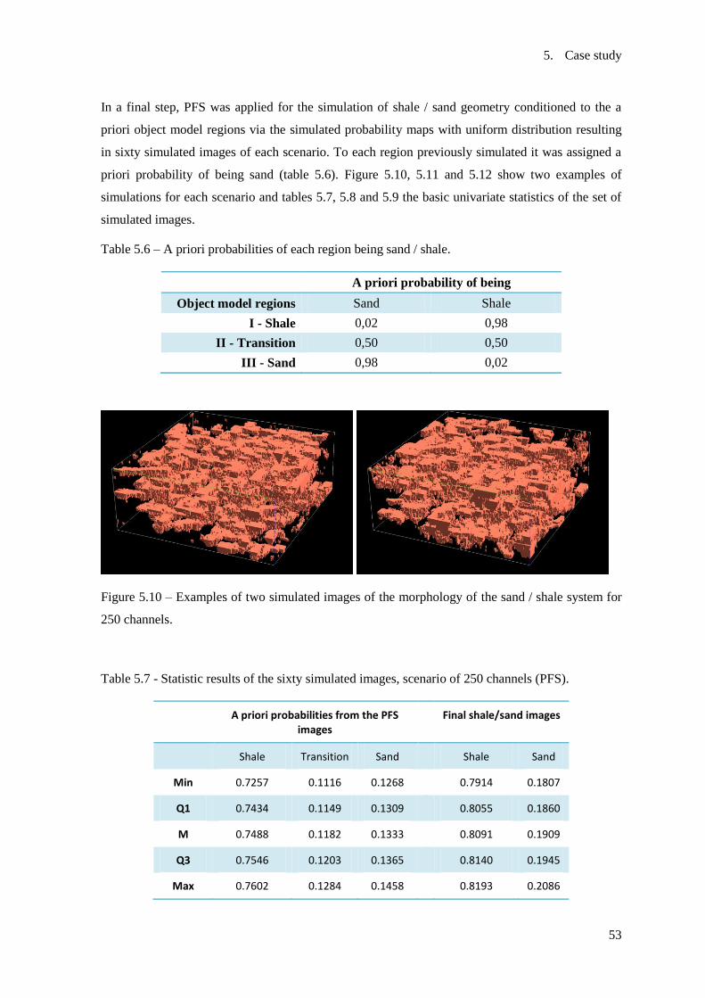
5. Case study
53
In a final step, PFS was applied for the simulation of shale / sand geometry conditioned to the a
priori object model regions via the simulated probability maps with uniform distribution resulting
in sixty simulated images of each scenario. To each region previously simulated it was assigned a
priori probability of being sand (table 5.6). Figure 5.10, 5.11 and 5.12 show two examples of
simulations for each scenario and tables 5.7, 5.8 and 5.9 the basic univariate statistics of the set of
simulated images.
Table 5.6 – A priori probabilities of each region being sand / shale.
A priori probability of being
Object model regions Sand Shale
I - Shale 0,02 0,98
II - Transition 0,50 0,50
III - Sand 0,98 0,02
Figure 5.10 – Examples of two simulated images of the morphology of the sand / shale system for
250 channels.
Table 5.7 - Statistic results of the sixty simulated images, scenario of 250 channels (PFS).
A priori probabilities from the PFS images
Final shale/sand images
Shale Transition Sand Shale Sand
Min 0.7257 0.1116 0.1268 0.7914 0.1807
Q1 0.7434 0.1149 0.1309 0.8055 0.1860
M 0.7488 0.1182 0.1333 0.8091 0.1909
Q3 0.7546 0.1203 0.1365 0.8140 0.1945
Max 0.7602 0.1284 0.1458 0.8193 0.2086

5. Case study
54
Figure 5.11 – Examples of two simulated images of the morphology of the sand / shale system for
500 channels (initial width).
Table 5.8 - Statistic results of the sixty simulated images, scenario of 500 channels (PFS).
A priori probabilities from the PFS images
Final shale/sand images
Shale Transition Sand
Shale Sand
Min 0.5556 0.2063 0.1995
0.6594 0.3126
Q1 0.5684 0.2129 0.2071
0.6706 0.3204
M 0.5742 0.2161 0.2106
0.6752 0.3248
Q3 0.5789 0.2179 0.2142
0.6796 0.3294
Max 0.5914 0.2266 0.2178
0.6874 0.3406
Figure 5.12 – Examples of two simulated images of the morphology of the sand / shale system for
500 channels (width / 2).
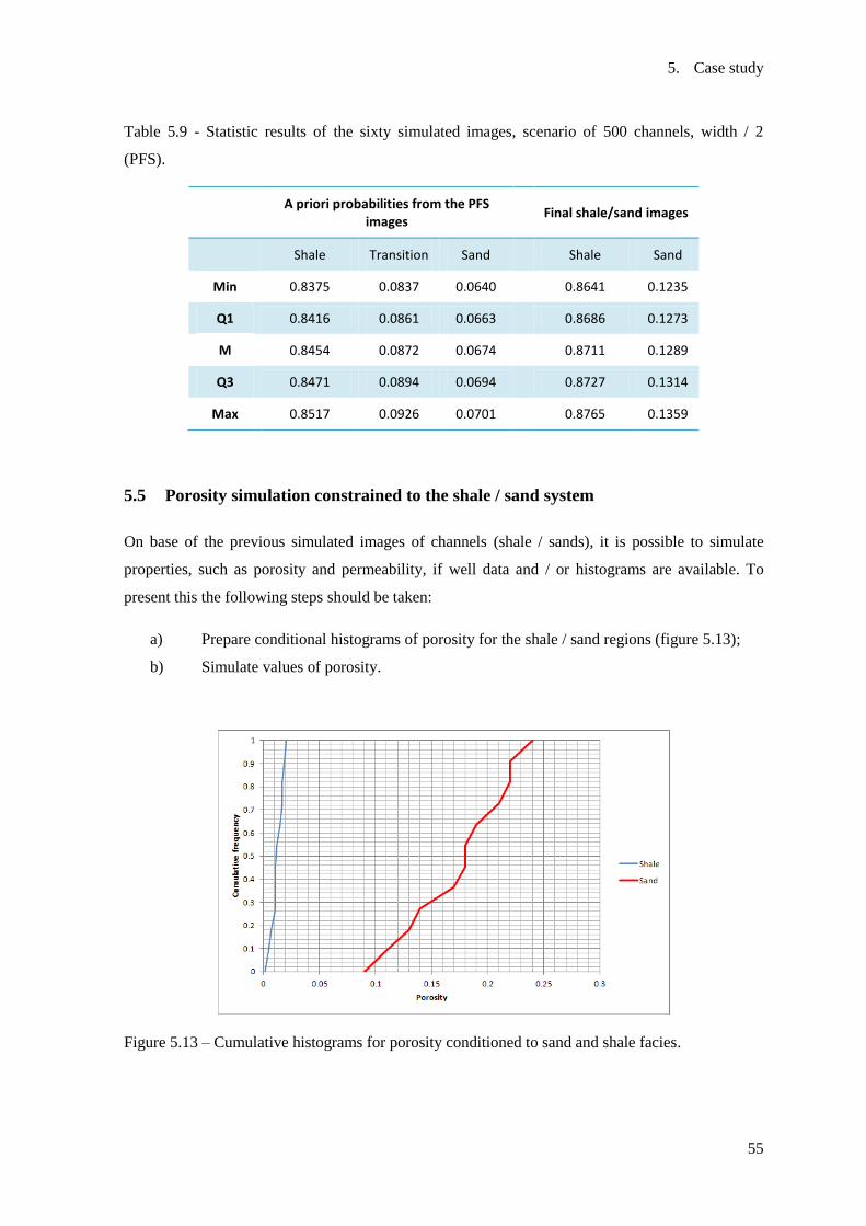
5. Case study
55
Table 5.9 - Statistic results of the sixty simulated images, scenario of 500 channels, width / 2
(PFS).
A priori probabilities from the PFS images
Final shale/sand images
Shale Transition Sand
Shale Sand
Min 0.8375 0.0837 0.0640
0.8641 0.1235
Q1 0.8416 0.0861 0.0663
0.8686 0.1273
M 0.8454 0.0872 0.0674
0.8711 0.1289
Q3 0.8471 0.0894 0.0694
0.8727 0.1314
Max 0.8517 0.0926 0.0701
0.8765 0.1359
5.5 Porosity simulation constrained to the shale / sand system
On base of the previous simulated images of channels (shale / sands), it is possible to simulate
properties, such as porosity and permeability, if well data and / or histograms are available. To
present this the following steps should be taken:
a) Prepare conditional histograms of porosity for the shale / sand regions (figure 5.13);
b) Simulate values of porosity.
Figure 5.13 – Cumulative histograms for porosity conditioned to sand and shale facies.
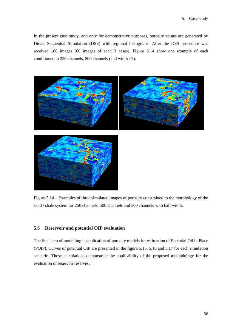
5. Case study
56
In the present case study, and only for demonstrative purposes, porosity values are generated by
Direct Sequential Simulation (DSS) with regional histograms. After the DSS procedure was
received 180 images (60 images of each 3 cases). Figure 5.14 show one example of each
conditioned to 250 channels, 500 channels (and width / 2).
Figure 5.14 – Examples of three simulated images of porosity constrained to the morphology of the
sand / shale system for 250 channels, 500 channels and 500 channels with half width.
5.6 Reservoir and potential OIP evaluation
The final step of modelling is application of porosity models for estimation of Potential Oil in Place
(POIP). Curves of potential OIP are presented in the figure 5.15, 5.16 and 5.17 for each simulation
scenario. These calculations demonstrate the applicability of the proposed methodology for the
evaluation of reservoir reserves.

5. Case study
57
Figure 5.15 – Potential OIP curves the 250 channels scenario.
Figure 5.16 – Potential OIP curves the 500 channels scenario.
Figure 5.17 – Potential OIP curves the 500 channels, width /2 scenario.

5. Case study
58
5.7 Discussion
To discuss the results it is presented first a set of figures illustrating partial and final results in
levels and cross-sections of the three scenarios (figures 5.18, 5.19 and 5.20)
Boole
an m
odel
PFS m
odel
Poro
sity
Figure 5.18 – Comparative results of one simulated image for (left) level and (right) cross-section
for scenario of 250 channels.

5. Case study
59
Boole
an m
odel
PFS m
odel
Poro
sity
Figure 5.19 – Comparative results of one simulated image for (left) level and (right) cross-section
for scenario of 500 channels.
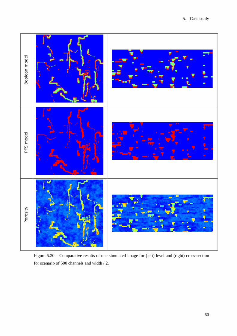
5. Case study
60
Boole
an m
odel
PFS m
odel
Poro
sity
Figure 5.20 – Comparative results of one simulated image for (left) level and (right) cross-section
for scenario of 500 channels and width / 2.

5. Case study
61
The sequence of results shows the follows:
Boolean model
a) From top to bottom, the shape of the channels is a half-ellipse.
b) Channels of the figure 5.8 are the same in number of the figure 5.7 but with half of the
width, which is clearly observed.
c) Transition blocks in red are at both sides of the channel and at bottom. They were
computed as 50% of the width and height.
d) The average length of the channels according the histogram of figure 5.1 is 2280m and the
computed average of the simulated channels is always approximately 10% lower. This is
explained because during growing process some channels reach the boundaries of the
reservoir in both directions and therefore in these cases the total length of these channels is
lower than the simulated from the histogram.
e) Channels vary in width and height according the simulated values showed in figure 5.4 and
5.5.
f) The entire network of channels follows from top to bottom the same orientation map which
can be improved for realistic reservoirs if different images are taken into account in depth;
g) Proportions of each phase are similar for the different realizations (15). When the number
of channels is multiplied by two (from 250 to 500), the proportion of sand are not
multiplied by two, but for a factor lower which can be explained by the reservoir
boundaries. When the width is subdivided by two the proportion of sands is much lower
probably due to the approximation between the size of each block and the width of the
channels.
PFS post-processing
a) Final simulated images follow the patterns of the Boolean models but the PFS post-
processing (in average only 2% of the a priori shale and sand regions are converted to
another) adds realism in the transition between shale and sands conditioned to a variogram
model;
b) Statistics of the final simulated images are in accordance with the expected values obtained
from the a priori probabilities from the PFS images (left columns of the tables 5.7, 5.8 and
5.9 and the a priori probability values of table 5.6). For instance for scenario of 500
channels, width /2:
Channels proportion: 0,8454 x 0,02 + 0,0872 x 0,50 + 0,0674 x 0,98 = 0,1266 (0,1289)
Sands proportion: 0,8454 x 0,98 + 0,0872 x 0,50 + 0,0674 x 0,02 = 0,8734 (0,8711)

5. Case study
62
Porosity
a) Simulated values of porosity are conditioned to sand and shale reference histograms via
direct sequential simulation with local histograms;
b) Direct sequential simulation with local histograms enables the simulation of porosity for
both facies in one unique step, instead of the two steps of the classical approach.

6. Final remarks
63
6. Final remarks
Recent news of searching alternative sources of energy show the critical situation of oil and gas
industry: the majority of oil fields are in mature phases of exploitation (including enhanced oil
recovery), others are located in extreme conditions (for instance, in off-shores at high depths), and
therefore the prospection and exploitation requires more significant investments. In such conditions
the only answer is to develop new modelling methodologies to deal with these new conditions.
In this work it was presented an innovative methodology of simulating 3D stochastic images of the
morphology of fluvial sand channels reservoirs. For testing this methodology it was used synthetic
data from a hypothetical channel sand reservoir and real porosity histograms from a Middle East
reservoir. This type of reservoirs is a particular challenge for modelling, because of a complex
geometry and sedimentological and structural heterogeneities.
In order to obtain a realistic model, the proposed methodology encompasses first the development
of a Boolean or object model followed by a post-processing geostatistical algorithm (Probability
Field Simulation). The combination of both algorithms enables to impose size statistics of the
channels such as length, width and height and a variogram model. Moreover, the methodology
generates a set of equally probable scenarios of the geometry of the sand / shale (channel / not
channel) system. These morphological images can be, in a second step, filled with petrophysical
properties values, such as porosity and permeability. For illustration purposes, porosity was
generated by Direct Sequential Simulation with local histograms of the two regions. The final step
of modelling was application of porosity models for estimation of Potential Oil in Place (POIP).
These calculations demonstrate the applicability of the proposed methodology for the evaluation of
reservoir reserves.
The obtained results for three scenarios of channels (low density, high density, and high density
with thin channels) showed advantages relatively to other methods:
a) Boolean model impose statistics of shape (half-ellipse section), sizes and local orientation
in a very efficient way;
b) Post-processing by Probability Field Simulation transforms the previous morphology
according a variogram model adding realism;
c) Implementation of the Direct Sequential Simulation with local histograms enables the
simulation of properties for both facies in one unique step, instead of the two steps of the
classical approach.
7. References
64
7. REFERENCES
Almeida, A., Journel, A., 1994. Joint simulation of multiple variables with a Markov-type
corregionalization model. Mathematical geology 26(5): 565-588.
Almeida, J.A., 1999. Use of geostatistical models to improve reservoir description and flow
simulation in heterogeneous oil fields. PhD thesis IST - 161.
Almeida, J.A., Barbosa, S. 2008. 3D stochastic simulation of fracture networks conditioned both to
field observations and a linear fracture density. Proceedings of the eighth international geostatistics
congress, Santiago do Chile: 129-136.
Almeida, J.A., 2010. Stochastic simulation methods for characterization of lithoclasses in carbonate
reservoirs. Earth Science Reviews, (101), 3-4: 250-270.
Basic Petroleum Geology and Log Analysis, 2001, Hallibuton: 28-32.
Compton, R.R., 1985. Geology in the Field. John Wiley and Sons, New York - 398.
Deutsch, C.V., Journel, A., 1992. GSLIB: Geostatistical Software Library and User’s Guide.
Oxford University Press, Stanford.
Deustch, C.V., Wang, L., 1996. Hierarchical object based stochastic modeling of fluvial reservoirs.
Mathematical Geology, v. 28:857-880.
Eaves E., 1976. Citronelle oil field, Mobile country, Alabama. Am Assos Petrol Geol Mem 16:
259-275.
Elliot L., 1989. The Surat and Bowen basins. Aust Petrol Explor Assoc J 29: 398-416.
Fritz, W., Moore, J., 1988. Exercises in Physical Stratigraphy and Sedimentology. John Wiley and
Sons, USA - 221.
Froidevaux, R., 1993. Probability Field Simulation, in A. Soares (ed), Geostatistics Troia’92,
Kluwer Academic Pub., Dordrecht, 1: 73-84.
Goovaerts, P., 1997. Geostatistics for Natural Resources Evaluation. Oxford University Press, New
York - 483.
Holden, L., Hauge, R., Skare, O., Skorstad, A., 1998. Modeling of fluvial reservoirs with object
models. Mathematical Geology, 30: 473-496.
Hu, L.Y., Chugunova, T., 2008. Multiple-point geostatistics for modeling subsurface heterogeneity:
a comprehensive review. Water Resources Research; 44: W11413.
7. References
65
Keogh, K., 2007. Sequence stratigraphy and 3-D modelling of the East Pennine Coalfield, UK: a
deterministic and stochastic approach. PhD thesis, University of Liverpool, UK - 281.
Leeder, M., 1999. Sedimentology and Sedimentary Basins: from turbulence to tectonics. Blackwell
Science Ltd - 592.
Lorenz J.C., Warpinski N.R., Branagan P.T., 1991. Subsurface characterization of Mesaverde
reservoirs in Colorado: geophysical and reservoir-engineering cheks on predictive sedimentology.
Soc Econ Paleontol Mineral Conc Sedimentol Paleontol 3: 57-79.
Luis, J., Almeida, J.A., 1997. Stochastic Characterization of Fluvial Sand Channels, Geostatistics
Wollongong’96, Volume 1, eds. E. Y. Baafi and N. A. Schofield. Kluwer Academic Publ.,
Netherlands: 477-488.
Lyons P.L., Dobrin M.B., 1972. Seismic exploration for stratigraphic traps. Am Assos Petrol Geol
Mem 16:225-243.
Mariethoz, G., Kelly, B.F.J., 2011. Modelling complex geological structures with elementary
training images and transform-invariant distances. Water Resources Research; 47: W07527.
Mata-Lima, H., 2008. Reservoir characterisation with iterative direct sequential co-simulation:
integrating fluid dynamic data into stochastic model. Journal of Petroleum Science and Engineering
doi: 10.1016/j. petrol.2008.07.003.
Matheron G., Beucher H, Fouquet, C., Galli A., Guerrilot D., Ravenne C., 1987. Conditional
simulation of the geometry of fluvio-deltaic reservoirs. In: SPE Annual Technical Conference and
Exhibition, 62, Dallas-TX: 123-130, SPE #16753.
Miall, A., 1996. The geology of fluvial deposits: sedimentary facies, basin analysis, and petroleum
geology. Springer-Verlag Berlin Heidelberg - 582.
Neuendorf, K., Mehl, J., Jackson, J., eds., 2005. Glossary of Geology. American Geological
Institute. Alexandria, Virginia - 800.
North, F., 1985. Petroleum Geology, University Press, Cambridge.
Nunes, R., Almeida, J.A., 2010. Parallelization of sequential Gaussian, indicator and direct
simulation algorithms. Computers & Geosciences, vol. 36: 1042-1052.
Peredo, O., Ortiz, J.M., 2011. Parallel implementation of simulated annealing to reproduce
multiple-point statistics. Computers and geosciences. 37: 1110-21.
Reading, H., 1996. Sedimentary Environments: Processes, Facies and Stratigraphy. Department of
Earth Sciences, University of Oxford, Third Edition - 688.
Reynolds D.W., Vincent J.K., 1972. Midland gas field, western Kentucky. Am Assos Petrol Geol
Mem 16:585-598.

7. References
66
Roxo, S., 2011. Integração de informação secundária na modelação geoestatistica da qualidade de
solos em locais potencialmente contaminados. Aplicação à área subjacente de uma antiga refinaria.
MsC Thesis. FCT-UNL - 64.
Soares, A., 1990. Geostatistical estimation of orebody geometry: morphological kriging.
Mathematical Geology 22(7): 787-802.
Soares, A., 2001. Direct Sequential Simulation and Cosimulation. Mathematical Geology, 33(8):
911–926.
Soares, A., 2006. Geoestatística para as Ciências daTerra e do Ambiente. IST Press - 214.
Srivastava, M., 1992. Reservoir Characterization with Probability Field Simulation, SPE Paper, N.
24753.
Strebelle, S., 2002. Conditional simulation of complex geological structures using multiple-point
geostatistics. Mathematical Geology. 34: 1-22.
Vargas-Guzmnan, J., Al-Qassab, H., 2006. Spatial conditional simulation of facies objects for
modelling complex clastic reservoirs. Journal of Petroleum Science and Engineering 54 (1-2): 1-9.
Weber, K.J., 1986. How heterogeneity affects oil recovery. Academic Press: 487-566.
Weber, K.J., Van Geuns L.C., 1990. Framework for constructing clastic reservoir simulation
models. J Petrol Technol 42: 1248-1253.
Wilson, W., Moore, J., 2003. Glossary of Hydrology. American Geological Institute, Springer -
248.
Woncik J., 1972. Recluse field, Campbell Country, Wyoming. Am Assos Petrol Geol Mem 16:376-
382.
Wood J.M., Hopkins J.C., 1992. Traps associated with paleovalleys and interfluves in an
unconformity bounded sequence: Lower Cretaceous Glauconitic Member, southern Alberta,
Canada. Am Assoc Petrol Geol Bull 76: 904-926.
Yinan Q., Peihua X., Jingsiu X., 1987. Fluvial sandstone bodies as hydrocarbon reservoirs in lake
basins. Soc Econ Paleontol Mineral Spec Publ 39:329-342.