ACTAUNIVERSITATIS

UPSALIENSISUPPSALA

2016

Digital Comprehensive Summaries of Uppsala Dissertationsfrom the Faculty of Science and Technology 1376

Stochastic Simulation of MultiscaleReaction-Diffusion Models via FirstExit Times

LINA MEINECKE

ISSN 1651-6214ISBN 978-91-554-9582-4urn:nbn:se:uu:diva-284085

Dissertation presented at Uppsala University to be publicly examined in ITC 2446,Lägerhyddsvägen 2, Uppsala, Friday, 10 June 2016 at 10:15 for the degree of Doctor ofPhilosophy. The examination will be conducted in English. Faculty examiner: Reader RamonGrima (University of Edinburgh).

AbstractMeinecke, L. 2016. Stochastic Simulation of Multiscale Reaction-Diffusion Models viaFirst Exit Times. Digital Comprehensive Summaries of Uppsala Dissertations from theFaculty of Science and Technology 1376. 53 pp. Uppsala: Acta Universitatis Upsaliensis.ISBN 978-91-554-9582-4.

Mathematical models are important tools in systems biology, since the regulatory networks inbiological cells are too complicated to understand by biological experiments alone. Analyticalsolutions can be derived only for the simplest models and numerical simulations are necessary inmost cases to evaluate the models and their properties and to compare them with measured data.

This thesis focuses on the mesoscopic simulation level, which captures both, space dependentbehavior by diffusion and the inherent stochasticity of cellular systems. Space is partitioned intocompartments by a mesh and the number of molecules of each species in each compartmentgives the state of the system. We first examine how to compute the jump coefficients fora discrete stochastic jump process on unstructured meshes from a first exit time approachguaranteeing the correct speed of diffusion. Furthermore, we analyze different methods leadingto non-negative coefficients by backward analysis and derive a new method, minimizing boththe error in the diffusion coefficient and in the particle distribution.

The second part of this thesis investigates macromolecular crowding effects. A highpercentage of the cytosol and membranes of cells are occupied by molecules. This impedes thediffusive motion and also affects the reaction rates. Most algorithms for cell simulations areeither derived for a dilute medium or become computationally very expensive when appliedto a crowded environment. Therefore, we develop a multiscale approach, which takes themicroscopic positions of the molecules into account, while still allowing for efficient stochasticsimulations on the mesoscopic level. Finally, we compare on- and off-lattice models on themicroscopic level when applied to a crowded environment.

Keywords: computational systems biology, diffusion, first exit times, unstructured meshes,reaction-diffusion master equation, macromolecular crowding, excluded volume effects, finiteelement method, backward analysis, stochastic simulation

Lina Meinecke, Department of Information Technology, Division of Scientific Computing, Box337, Uppsala University, SE-751 05 Uppsala, Sweden.

© Lina Meinecke 2016

ISSN 1651-6214ISBN 978-91-554-9582-4urn:nbn:se:uu:diva-284085 (http://urn.kb.se/resolve?urn=urn:nbn:se:uu:diva-284085)

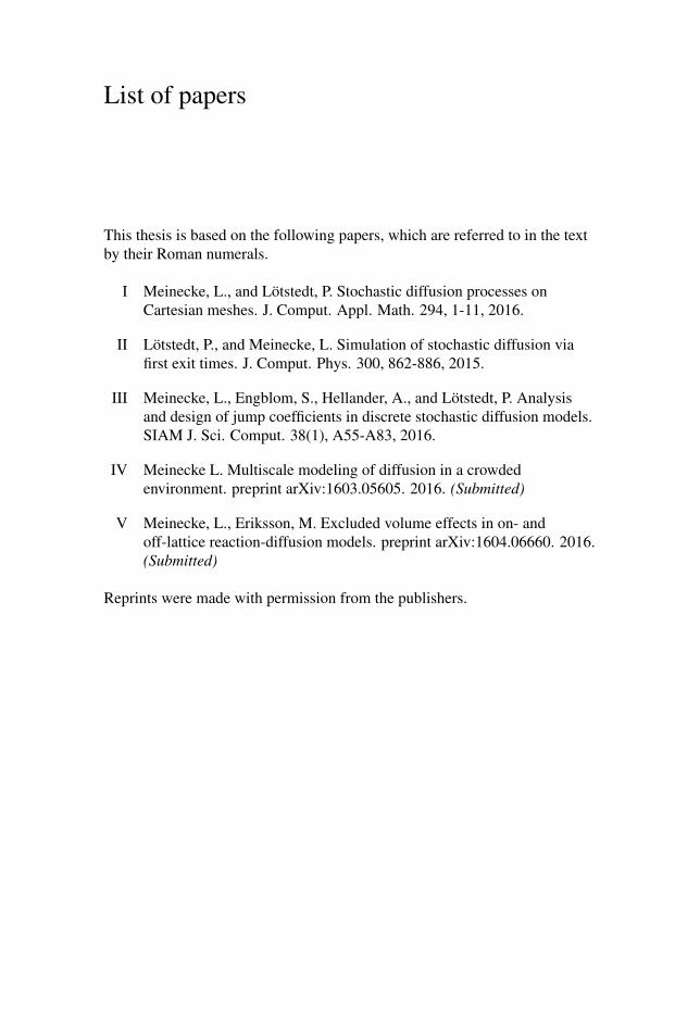
List of papers

This thesis is based on the following papers, which are referred to in the text

by their Roman numerals.

I Meinecke, L., and Lötstedt, P. Stochastic diffusion processes on

Cartesian meshes. J. Comput. Appl. Math. 294, 1-11, 2016.

II Lötstedt, P., and Meinecke, L. Simulation of stochastic diffusion via

first exit times. J. Comput. Phys. 300, 862-886, 2015.

III Meinecke, L., Engblom, S., Hellander, A., and Lötstedt, P. Analysis

and design of jump coefficients in discrete stochastic diffusion models.

SIAM J. Sci. Comput. 38(1), A55-A83, 2016.

IV Meinecke L. Multiscale modeling of diffusion in a crowded

environment. preprint arXiv:1603.05605. 2016. (Submitted)

V Meinecke, L., Eriksson, M. Excluded volume effects in on- and

off-lattice reaction-diffusion models. preprint arXiv:1604.06660. 2016.

(Submitted)

Reprints were made with permission from the publishers.

Contents

1 Introduction . . . . . . . . . . . . . . . . . . . . . . . . . . . . . . . . . . . . . . . . . . . . . . . . . . . . . . . . . . . . . . . . . . . . . . . . . . . . . . . . . . . . . . . . . . . . . . . . . . 7

2 Reaction-diffusion modeling . . . . . . . . . . . . . . . . . . . . . . . . . . . . . . . . . . . . . . . . . . . . . . . . . . . . . . . . . . . . . . . . . . . . 10

2.1 Macroscopic model . . . . . . . . . . . . . . . . . . . . . . . . . . . . . . . . . . . . . . . . . . . . . . . . . . . . . . . . . . . . . . . . . . . . . . . . 10

2.2 Mesoscopic model . . . . . . . . . . . . . . . . . . . . . . . . . . . . . . . . . . . . . . . . . . . . . . . . . . . . . . . . . . . . . . . . . . . . . . . . . . 11

2.2.1 Well-mixed systems: the chemical master equation . . . . . 11

2.2.2 The reaction-diffusion master equation . . . . . . . . . . . . . . . . . . . . . . . . . 13

2.2.3 The stochastic simulation algorithm . . . . . . . . . . . . . . . . . . . . . . . . . . . . . . 15

2.3 Microscopic model . . . . . . . . . . . . . . . . . . . . . . . . . . . . . . . . . . . . . . . . . . . . . . . . . . . . . . . . . . . . . . . . . . . . . . . . . 16

2.3.1 First passage kinetic Monte Carlo algorithms . . . . . . . . . . . . . . . 17

2.3.2 Cellular automata . . . . . . . . . . . . . . . . . . . . . . . . . . . . . . . . . . . . . . . . . . . . . . . . . . . . . . . . . . . . . 19

2.4 Connection between levels . . . . . . . . . . . . . . . . . . . . . . . . . . . . . . . . . . . . . . . . . . . . . . . . . . . . . . . . . . . . 20

3 Jump coefficients on unstructured meshes . . . . . . . . . . . . . . . . . . . . . . . . . . . . . . . . . . . . . . . . . . . . . . . 21

3.1 FEM discretization . . . . . . . . . . . . . . . . . . . . . . . . . . . . . . . . . . . . . . . . . . . . . . . . . . . . . . . . . . . . . . . . . . . . . . . . . 22

3.2 The FET approach for mesoscopic jump rates . . . . . . . . . . . . . . . . . . . . . . . . . . . . . 22

3.2.1 Local FET . . . . . . . . . . . . . . . . . . . . . . . . . . . . . . . . . . . . . . . . . . . . . . . . . . . . . . . . . . . . . . . . . . . . . . . . 22

3.2.2 Global FET . . . . . . . . . . . . . . . . . . . . . . . . . . . . . . . . . . . . . . . . . . . . . . . . . . . . . . . . . . . . . . . . . . . . . . 24

3.3 Error analysis . . . . . . . . . . . . . . . . . . . . . . . . . . . . . . . . . . . . . . . . . . . . . . . . . . . . . . . . . . . . . . . . . . . . . . . . . . . . . . . . . . 27

3.3.1 Backward error . . . . . . . . . . . . . . . . . . . . . . . . . . . . . . . . . . . . . . . . . . . . . . . . . . . . . . . . . . . . . . . . 27

3.3.2 Computing γ0 . . . . . . . . . . . . . . . . . . . . . . . . . . . . . . . . . . . . . . . . . . . . . . . . . . . . . . . . . . . . . . . . . . . 27

3.3.3 Minimal backward error . . . . . . . . . . . . . . . . . . . . . . . . . . . . . . . . . . . . . . . . . . . . . . . . . . 28

4 Macromolecular crowding . . . . . . . . . . . . . . . . . . . . . . . . . . . . . . . . . . . . . . . . . . . . . . . . . . . . . . . . . . . . . . . . . . . . . . . . 30

4.1 Microscopic model . . . . . . . . . . . . . . . . . . . . . . . . . . . . . . . . . . . . . . . . . . . . . . . . . . . . . . . . . . . . . . . . . . . . . . . . . 31

4.1.1 CA and crowding . . . . . . . . . . . . . . . . . . . . . . . . . . . . . . . . . . . . . . . . . . . . . . . . . . . . . . . . . . . . . 31

4.2 Mesoscopic model . . . . . . . . . . . . . . . . . . . . . . . . . . . . . . . . . . . . . . . . . . . . . . . . . . . . . . . . . . . . . . . . . . . . . . . . . . 33

4.2.1 Multiscale approach . . . . . . . . . . . . . . . . . . . . . . . . . . . . . . . . . . . . . . . . . . . . . . . . . . . . . . . . 34

4.3 Macroscopic model . . . . . . . . . . . . . . . . . . . . . . . . . . . . . . . . . . . . . . . . . . . . . . . . . . . . . . . . . . . . . . . . . . . . . . . . 36

5 Summary . . . . . . . . . . . . . . . . . . . . . . . . . . . . . . . . . . . . . . . . . . . . . . . . . . . . . . . . . . . . . . . . . . . . . . . . . . . . . . . . . . . . . . . . . . . . . . . . . . . . 37

6 Authors contribution . . . . . . . . . . . . . . . . . . . . . . . . . . . . . . . . . . . . . . . . . . . . . . . . . . . . . . . . . . . . . . . . . . . . . . . . . . . . . . . . . . 40

7 Summary in Swedish . . . . . . . . . . . . . . . . . . . . . . . . . . . . . . . . . . . . . . . . . . . . . . . . . . . . . . . . . . . . . . . . . . . . . . . . . . . . . . . . . 41

8 Acknowledgments . . . . . . . . . . . . . . . . . . . . . . . . . . . . . . . . . . . . . . . . . . . . . . . . . . . . . . . . . . . . . . . . . . . . . . . . . . . . . . . . . . . . . 43

References . . . . . . . . . . . . . . . . . . . . . . . . . . . . . . . . . . . . . . . . . . . . . . . . . . . . . . . . . . . . . . . . . . . . . . . . . . . . . . . . . . . . . . . . . . . . . . . . . . . . . . . . 44

1. Introduction

A cell is regarded as the true biological

atom. Nothing is living but cells, or what

can be directly traced back to cells.

George Henry Lewes

Cells are the building blocks of all living organisms, they contain the ge-

netic material that defines which species we are. Prokaryotes, such as bacte-

ria, are simple single cell organisms without a nucleus or membrane bound

organelles. Mammals and other higher organisms on the other hand consist

of trillions of complex eukaryotic cells, which have a nucleus containing the

DNA, complicated membranes and specialized organelles such as mitochon-

dria and the Golgi apparatus [1]. Although every cell in our body is genetically

identical they are still able to specialize and perform very different tasks. The

specialization during embryonic development or "simple" cell division and the

effect of aging are still not fully understood and remain open problems in bi-

ology and medicine [81]. Imaging techniques have enabled biologists to study

the cellular machinery and to understand how the genetic material is encoded

on the DNA, how it is copied during cell division, and how it is first transcribed

into mRNA and then translated into proteins. Gene transcription is regulated

by the binding of transcription factors to the DNA that either repress or pro-

mote the binding of RNA polymerase to start producing the mRNA template

for translation.

The aim of systems biology is now to understand how gene regulation en-

ables complex cell behavior such as cell division, stem cell differentiation and

embryonic development. Mathematical modeling is a crucial tool to under-

stand these complex mechanisms. The first requirement on the mathematical

model is agreement with existing experimental data. But more importantly,

the model is only useful if it allows us to obtain novel insight into cell be-

havior. These findings can then be validated by new biological experiments,

which further refine the model. Accurate mathematical models are often too

complex to analyze analytically and numerical simulations, so called in silicoexperiments, are needed. Due to the complexity of the reaction networks, we

can in general only simulate a small subset of the molecules present inside

cells [43], although a first attempt to simulate a complete cell - a bacterium

with 525 genes - has been made [75].

The mathematical models in use today do not follow a unified mathemati-

cal framework. Instead, they span a wide range of accuracy and computational

7

cost. Many models assume the molecules to be well-mixed and equally dis-

tributed inside the cell and hence allow for the simplification that only reaction

events have to be considered. Yet, cells are spatially organized objects with a

cell membrane where extracellular particles bind, so that a signal is released

into the cytosol and moves to the nucleus, or cells change their geometry dur-

ing cell division. Hence space-dependent models are essential to capture many

interesting cellular phenomena [39, 120]. Molecules can move e.g. by active

transport or by Brownian motion. The latter is the random movement of parti-

cles due to their thermal energy and their multiple collisions with the smaller

solvent molecules. As a result of this random walk molecules diffuse inside

the cell from higher to lower concentrations. Reaction-diffusion processes are

very prominent in modeling cellular systems, with the most famous example

being the equations for pattern formation presented by Turing [125] in 1952.

Another important detail of cellular processes are random fluctuations. As

mentioned, the molecules’ diffusive movement is due to their random walk and

both intrinsic and extrinsic noise render every reaction event random [119].

Since important molecules inside the cell are often present only at very low

copy numbers (there is e.g. only one copy of DNA), the law of large numbers

that holds for chemical systems with large molecule counts is not applicable

inside cells and stochastic models are more accurate than simpler determinis-

tic models [79, 90, 93]. The molecular fluctuations do not only lead to hetero-

geneity in the cell behavior, but cells also exploit the noise to stabilize their

reaction networks by stochastic focusing [95, 103].

In this thesis we will present three levels of reaction-diffusion modeling:

macroscopic models (deterministic), mesoscopic models (stochastic and dis-

crete in space) and microscopic models (stochastic and continuous in space).

The research presented in Papers I-V contributes to developing accurate and

computationally efficient algorithms for the stochastic simulation of the molec-

ular diffusion on the mesoscopic level. Diffusion is here modeled by a discrete

jump process, and in order to accurately represent the complicated geometries

inside cells an unstructured discretization of the domain is favorable. On these

unstructured meshes, however, the traditional method of computing the jump

coefficients might lead to negative and unphysical jump rates. Another short-

coming is that molecules are modeled as point particles, which changes the

reaction-diffusion dynamics as compared to more physical models where the

molecules occupy volume and interact through hard sphere repulsion. To ad-

dress these two issues we:

• Derive the coefficients for the discrete stochastic jump process on an

unstructured mesh such that they preserve the speed of diffusion (Papers

I and II).

• Estimate and minimize the error introduced by different numerical tech-

niques to obtain non-negative jump propensities (Paper III).

• Establish a multiscale model to efficiently simulate reaction-diffusion

processes including the excluded volume effects inside cells (Paper IV).

8

• Compare on- and off-lattice particle based methods for reaction-diffu-

sion simulations in the crowded cell environment (Paper V).

The rest of this thesis is organized as follows. In Chapter 2 we review the dif-

ferent reaction-diffusion models existing on the three levels of accuracy, how

they resolve space, how they relate to each other, and what software is avail-

able for their computation. The mesoscopic level with an unstructured space

discretization is presented in more detail in Chapter 3, where we derive a first

exit time approach to compute the jump rates such that the speed of diffusion

is modeled accurately. We then perform backward analysis to estimate the

error in unstructured jump processes and minimize it with a new set of jump

coefficients. Chapter 4 is a further step towards more accurate models of cells,

where we take molecular crowding effects in the cytosol or on the membrane

into account, and present a multiscale model for stochastic reaction-diffusion

simulations in such an environment. We summarize this thesis and the contri-

butions of the papers in Chapter 5.

The mathematical notation in this thesis is as follows: the time derivative

of a quantity c(t) is denoted by ct(t), x ∈ Rn is a n-dimensional vector with

components xi, and capital bold face letters M denote matrices. For vectors

‖x‖p denotes the vector norm in �p and ‖M‖p its subordinate matrix norm.

9

2. Reaction-diffusion modeling

In this chapter we present three levels of reaction-diffusion modeling: the de-

terministic macroscopic level and the more detailed stochastic mesoscopic and

microscopic levels, along with how they relate to each other and when which

model is applicable.

2.1 Macroscopic model

The law of mass action [57] states that the rate of a chemical reaction is pro-

portional to the masses of the reacting species. Assuming mass action we can

derive the reaction rate equations (RREs), a system of deterministic ordinary

differential equations (ODEs) describing the time evolution of the concentra-

tions of well-mixed reacting species. Take e.g. the reversible binding with

association rate ka and dissociation rate kd

A+Bka�kd

C. (2.1)

Let a(t) be the concentration of the A molecules at time t and equivalently for

B and C, then by mass-action the change of concentration in time is governed

by these RREs

at(t) = −kaa(t)b(t)+ kdc(t),bt(t) = −kaa(t)b(t)+ kdc(t), (2.2)

ct(t) = kaa(t)b(t)− kdc(t).

A large set of analytic and computational tools exists to solve and analyze

these types of ODE systems.

If we assume that the cell is not a well-mixed system and we want to resolve

the diffusive motion of the molecules inside the volume Ω, then the concen-

tration of particles becomes a space-dependent quantity c(x, t) and its time

evolution is governed by the diffusion equation

ct(x, t) = γ0Δc(x, t), x ∈ Ω, (2.3)

with initial distribution c0 and reflecting or partially absorbing boundary con-

ditions on ∂Ω. Here, γ0 denotes the diffusion coefficient in a dilute medium.

10

These diffusive terms are then added to the system (2.2) for a reaction diffu-

sion model.

To solve (2.3) numerically we semi-discretize the equation in space with a

discretization matrix Dct(t) = Dc (2.4)

and then use an appropriate time stepping scheme. Possible space discretiza-

tion methods are the finite difference method (FDM) for a Cartesian discretiza-

tion or the finite volume method (FVM) and the finite element method (FEM)

for discretizations with unstructured meshes.

Describing the biological system by the RREs and diffusion equation is a

valid model when the molecules are abundant. In that case the concentra-

tions of molecules become continuous quantities and the system follows its

deterministic mean behavior. But, inside living cells individual species are

often only present at very low copy numbers, so that the discrete number of

molecules becomes the quantity of interest, which is a stochastic variable. As

a result, a stochastic model is often needed to capture cell biological processes

accurately [90, 103, 130], where the diffusion of single particles is modeled

as a random walk and reactions as random processes. In the limit of large

molecule numbers these models should in return converge to the deterministic

description in this section [83, 84].

We identify two levels of stochastic models, the mesoscopic (discrete in

space, continuous in time) and the microscopic (continuous in both space and

time).

2.2 Mesoscopic modelIn the mesoscopic model we describe the reaction-diffusion process by a con-

tinuous-time discrete-space Markov process. The state of the system is the

random vector containing the discrete number of molecules of each species

at time t. We first present the mesoscopic model for the well-mixed case and

then proceed to the spatially resolved case.

2.2.1 Well-mixed systems: the chemical master equation

Assume we have M different species that are well-mixed inside the domain

Ω, meaning that a randomly chosen molecule has the same probability to be

found in any equally sized subvolume [50]. The state vector of the system is

then Y(t) ∈ NM0 , where Yi(t) represents the number of molecules of species i

at time t. Let y(t) be one realization of the stochastic process. The species

can undergo R different reactions with stoichiometry vectors nr, each firing of

reaction r changes the state space by

ywr(y)−−−→ y−nr. (2.5)

11

For the reversible bimolecular reaction (2.1) and y(t) = (A(t),B(t),C(t)), the

two stoichiometry vectors are

n1 = (1,1,−1) and n2 = (−1,−1,1) (2.6)

for the forward and backward reactions respectively, and wr(y) are the propen-

sity functions, describing the rate at which the association and dissociation

reactions fire

w1(y(t)) = kaA(t)B(t) and w2(y(t)) = kdC(t). (2.7)

The state of the system at time t is then

y(t) = y(0)− r1(t)n1 − r2(t)n2, (2.8)

where r1(t) and r2(t) are counting processes, counting the number of forward

and backward reactions that have happened until t. Let P be a unit rate Pois-

son process. The counting process is then given by the random time change

representation [85]

r1(t) = P(∫ t

0kaA(t)B(t)dt

), (2.9)

and equivalently for r2(t). We can then show that the number of reactions

fulfills the Markov property [5]

p(r1(t +Δt)− r1(t) = 1|r1(s),s < t) = kaA(t)B(t)Δt +o(Δt), (2.10)

meaning that the probability for a reaction to happen only depends on the cur-

rent state and not on the past of the system. The reaction probability is further-

more proportional to the propensity function and the length of the infinitesimal

time interval. Consequently, the waiting time until the next reaction r occurs

is exponentially distributed with propensity wr(y). Let p(y, t) = p(y, t|y0, t0)be the probability density function (PDF) that the system is in state y at time

t given that it started in y0 at t0. Using Dynkin’s formula we can then show

that its time evolution is governed by the forward Kolmogorov equation or

chemical master equation (CME)

∂ p(y, t)∂ t

= Rp(y, t) =R

∑r=1

wr(y+nr)p(y+nr, t)−wr(y)p(y, t). (2.11)

This system of ODEs describes the probability distribution of the stochastic

process. It can be solved analytically for monomolecular reactions [72] or

simulated stochastically as presented in Section 2.2.3.

By choosing a fixed time step τ small enough, so that A(t) and B(t) can be

considered constant in τ we can approximate the integral in (2.9), and (2.8)

becomes

y(t + τ) = y(t)−P(kaA(t)B(t)τ)n1 −P(kdC(t)τ)n2. (2.12)

12

This approximate method is called τ-leaping and we will discuss in Sec-

tion 2.2.3 how it can be used to speed up stochastic simulations. Assuming that

the propensity wr � 1 we can further approximate the Poisson random num-

bers for the reaction count by a normal distribution N (wr,wr). This leads to

a stochastic differential equation (SDE) describing the reaction system, the so

called chemical Langevin equation (CLE). Using van Kampen’s system size

expansion [126] we can linearize the noise term to obtain the linear noise ap-

proximation (LNA), which describes the fluctuations around the mean value

with the variance scaling as the system size [56, 62]. Taking the full thermody-

namic limit, meaning that the concentrations remain constant, while both vol-

ume and number of molecules tend towards infinity, the stochastic terms be-

come negligible and the equations converge to the RREs describing the mean

value and equations for the higher order moments exist [30]. A comprehensive

summary of these models and the underlying physical assumptions is given in

the review [50].

2.2.2 The reaction-diffusion master equation

In this section we extend the well-mixed mesoscopic model to resolve space.

To this end, we first discretize space into N nodes xi with a space discretization

parameter h, and introduce dual grid cells (so called voxels) Vi with volume

Vi and centers xi, see Fig. 2.1. The state space is then extended to Y(t) ∈N

N×M0 , where Yi j denotes the number of molecules of species i located inside

voxel V j. Diffusion is modeled as a discrete jump process from a voxel Vi to

one of the neighboring voxels V j, which can be formulated analogously to a

monomolecular reaction

Aiλi j−→ A j, (2.13)

where Ai denotes an A molecule inside voxel Vi and λi j denotes the jump

coefficient for a jump from voxel Vi to V j. In Chapter 3 we will present how

to compute these jump coefficients, especially for unstructured meshes. The

propensity function for jumps by molecules of species k is

vi j(yki(t)) = λi jyki(t). (2.14)

Similar to the CME, we can state the diffusion master equation (DME)

∂ p(y, t)∂ t

=D p(y, t) =N

∑i=1

N

∑j=1

v ji(y+m ji)p(y+m ji, t)−vi j(y)p(y, t), (2.15)

where the transition vector m ji is zero except for m ji,i =−1 and m ji, j = 1.

We assume that the voxels are small enough, so that the molecules are well-

mixed inside and their positions are not resolved any further. Reactions are

13

Figure 2.1. The mesoscopic model for reaction-diffusion simulations on an unstruc-

tured mesh. The primal mesh (black) gives rise to the dual mesh, which creates the

voxels (blue). The state of the system is the discrete number of molecules (red and

grey) per voxel. The voxels are assumed to be small enough, so that the molecules

are well-mixed inside and can react (green arrow) according to the CME. Diffusion is

modeled by a discrete jump process from a voxel to a neighboring voxel (red arrows).

then described by local CMEs (2.11) inside each voxel:

Rp(y, t) =R

∑r=1

wr(y+nr)p(y+nr, t)−wr(y)p(y, t), (2.16)

with propensity functions wr(y·i) depending on the state y·i of voxel Vi. These

local propensity functions are similiar to those in (2.7), but need to be rescaled

according to the volume of the voxel and the type of the reaction:

Birth process: /0 → A wr(y·i) =Vikb,

Monomolecular reactions: C → A+B wr(y·i) = kd ·C(t),

Bimolecular reaction: A+B →C wr(y·i) =ka

Vi·A(t)B(t).

Note that more complicated reactions can be decomposed into subsequent

steps of these elementary reactions. Combining the CME for the space-depen-

dent case (2.16) and the diffusion master equation (2.15) leads to the reaction-

diffusion master equation (RDME):

∂ p(y, t)∂ t

= Rp(y, t)+D p(y, t). (2.17)

The solution of the DME converges towards that of the diffusion equation

(2.3) for a decreasing space discretization h → 0. A higher number of voxels,

however, also means that two molecules are less likely to be located within

the same voxel, where they can react. This leads to a decrease in the overall

bimolecular reaction rate for finer discretizations, until they are completely ne-

glected [69]. The CME furthermore assumes that that the molecules are dilute

14

in each voxel, which no longer holds for infinitesimally small voxels, invali-

dating the local CMEs. Different methods have been proposed to circumvent

this model problem of the RDME. In [70] the convergent RDME (cRDME)

is presented, where the molecules are allowed to react within a h-independent

reaction radius and do not need to be located in the same voxel. Other ap-

proaches include rescaling the reaction propensity to either accurately model

the mean binding time for two molecules [66, 67], the robustness of the steady

state [34] or matching the equilibration time of reversible reactions [38].

If there are only monomolecular reactions happening in the cell the CME

(and RDME) can be solved analytically [72], but for bimolecular reactions

the propensity functions wr are non-linear and there exists no analytic solu-

tion. A numerical solution is very costly and often unfeasible due to the high

dimension (N×M) of the state space. To overcome this curse of dimensional-

ity, attempts to reduce the dimensions have been made by projecting the state

space onto a smaller domain of interest [26, 31, 65, 71, 73, 99].

Instead of solving the master equation, a common method is to compute

sample paths from the CME or RDME and then compute statistics by a Monte

Carlo approach, as presented in the next section.

2.2.3 The stochastic simulation algorithm

In this section we present how to sample realizations of the stochastic process

Y(t). Using Monte Carlo methods we can then compute different moments,

such as the mean behavior and variance, and Bayesian approaches allow us

to regenerate the PDF. The algorithm to sample individual trajectories is gen-

erally known as the stochastic simulation algorithm (SSA), first proposed by

Gillespie in the 1970s [47, 48] and therefore also called the Gillespie algo-

rithm. A general guide to stochastic simulations and how to sample random

numbers from any distribution by inverse transform sampling is presented in

[33]. As mentioned above, the system is Markovian and therefore, the time

until reaction r happens is exponentially distributed with parameter wr. In the

direct method [48] we first compute the total propensity for any reaction to

happen w0 = ∑r wr and then sample a time for the next reaction. The proba-

bility for a reaction of type r is wr/w0, and the algorithm proceeds as follows.

Algorithm 1 Stochastic Simulation Algorithm (SSA)

1: Initialize y at t = 0.

2: Evaluate wr(y) and compute w0(y) = ∑r wr(y).3: Sample the time step τ for the next reaction to occur from the probability

density function w0e−w0(y)τ .

4: Sample which reaction r happens with probability wrw0

.

5: Update t := t + τ , y = y−nr.

6: Go to 2.

15

This is an exact method and it is straightforward to extend it to sample

the RDME by including the jumps as monomolecular reactions. But it be-

comes computationally expensive when computing many sample paths, since

we have to generate two random numbers in every time step. The next reaction

method (NRM) by Gibson and Bruck [45] initially generates the times when

each reaction is supposed to fire and then updates the times for those reac-

tions whose propensities were affected by previous reactions. Here, the reac-

tions are ordered in a priority queue, often implemented as a binary heap, and

one needs one new random number per reaction event. The next subvolume

method (NSM) [27] is the extension to the space-dependent RDME, where

reaction and diffusion events in a single subvolume are grouped together and

the NRM is then applied to the subvolumes, so that only the random times of

the affected subvolumes are resampled and reentered into the event queue.

To further gain efficiency there also exist approximate methods. One of

them is the τ-leaping method, first introduced in [49]. As mentioned in Sec-

tion 2.2.1 the idea is to keep the propensity functions constant for a sufficiently

small fixed time step τ and use a constant rate Poisson process to determine

how many reactions occurred. The risk is that τ is chosen too large and the

method becomes inaccurate or that too many reactions fire, such that the re-

sulting molecule number is negative, which is unphysical. On the other hand

choosing τ too small makes the method inefficient (even more expensive than

the SSA), since for a small τ many of the sampled Poisson random numbers

will be zero. This issue has been resolved in [16] by changing τ adaptively

and switching to the SSA for too small τ . Further improvements can be found

e.g. in [2, 17, 123].

The other advantage of the τ-leaping method is that it allows us to intro-

duce a nested grid of different time steps to perform a multilevel Monte Carlo

(MLMC) simulation, first introduced by Giles [46] for SDEs in finance and

adapted to the SSA in [3, 4]. The idea is to compute the mean value on dif-

ferent time discretization levels which are coupled in such a way that the total

variance is reduced and one hence needs fewer sample paths for a given accu-

racy. This approach has been extended to adaptive time steps and nested levels

of error, to efficiently simulate stiff reaction systems [18, 88].

2.3 Microscopic model

On the microscopic level we perform particle-based reaction-diffusion (PBRD)

simulations, where we follow individual molecules along their Brownian tra-

jectories and reactions happen with a certain probability when molecules come

close to each other. This is the finest modeling level considered in this thesis

and is inherently space-dependent.

There are two different methods for advancing the molecules in time. First,

Brownian dynamics (BD) simulations, where the Brownian trajectory of the

16

particles is discretized with a fixed time step Δt and random numbers are drawn

at each time step to sample how far the molecules move in each of the Carte-

sian directions

Δx =√

2γ0Δtξ , (2.18)

where ξ is a normally distributed random number N (0,1) and analogously

for Δy and Δz, since the Brownian motion is independent along coordinate

axes. Molecules that are within a predefined reaction radius σ of each other

react with a given probability during the time step Δt. This operator splitting

for the reaction and diffusion events introduces an error in the model. Exam-

ples of implementations of Brownian dynamics with a fixed time step Δt can

be found in the software packages Smoldyn [6, 7] and MCell [77, 118].

In the second method, called Green’s function reaction dynamics (GFRD)

[128, 127], the many body problem is decomposed into one- and two-body

problems. The probability distribution of the particles’ positions in these

smaller subsystems are analytically computable with Green’s functions. One

can either choose a time step Δt small enough, so that each pair or single

molecule has a very low probability to exit its surrounding protective domain

and to interact with other pairs/singles before Δt. Alterantively one can sample

the time until one of the protective domains is exited in a first passage kinetic

Monte Carlo simulation (FPKMC) [24, 102, 120], an exact method imple-

mented in the software ECell [124]. We will present the FPKMC approach

in more detail in Section 2.3.1. At each time step the positions and eventual

reactions are updated, the molecules are regrouped, and after defining new

protective domains a new next event time is sampled. This is an event-driven

approach with an adaptive time step Δt, and is computationally advantageous

for dilute systems with large protective domains, but when the system becomes

dense BD simulations start to outperform the GFRD approach.

Moreover, there are two models for how reaction events are handled. In

the volume reactivity model by Doi [22, 23] molecules are modeled as points

and react with each other with a prescribed probability, when they are in a re-

action radius of each other. In the contact reactivity or Smoluchowski model

[112] the particles are modeled as hard spheres and they react with a certain

probability when two spheres collide, represented by a reactive boundary con-

dition at the reaction radius σ for pair propagators in the GFRD approach.

The different software packages available for particle based simulations on

the microscopic scale are summarized and compared in [114].

2.3.1 First passage kinetic Monte Carlo algorithms

In this section we present how to compute the exit time distribution of a diffus-

ing molecule from a given domain ω . This domain can either be the protective

sphere or cube in the FPKMC algorithm (Fig. 2.2), or it can be used to com-

pute the mesoscopic jump rates as we will present in Chapter 3.

17

Δt

(a)

t

0 0.1 0.2 0.3 0.4

S(t)

0

0.2

0.4

0.6

0.8

1

(b)

Figure 2.2. (a) Illustration of the FPKMC algorithm with spherical and rectangular

protective domains. The FPKMC is an asynchronous event-driven algorithm where a

new time step Δt is chosen in each iteration. The blue shaded region illustrates the

solution to (2.19) for a given time t. (b) The survival probability S(t) of a diffusing

particle inside a protective domain, which is used to sample the next jump time Δt.

Let c(x, t) be the probability distribution for a diffusing molecule starting

in x0 at time t = 0 to be in x without leaving ω until time t, then

ct(x, t) = γ0Δc(x, t), x ∈ ω, (2.19)

c(x, t) = 0, x ∈ ∂ω,

c(x,0) = δx0,

where the homogeneous Dirichlet boundary condition models the particle’s

removal from the domain once it reaches the boundary, and δx0denotes the

Dirac delta function centered at x0. The survival probability of the particle

inside ω until time t is

S(t) =∫

ωc(x, t)dx. (2.20)

By Gauss’ formula the probability density pω(t) that the particle leaves ω at

t is given by

pω(t) =−∂S(t)∂ t

=−γ0

∫∂ω

n ·∇c(x(s), t)ds, (2.21)

with the outward normal n. The flux out of the volume ω is −γ0∇c ·n and the

conditional probability that the molecule leaves ω at point x given that the exit

occurs at time t is

j(x,x0, t) =−γ0n ·∇c(x,x0, t)

pω(t|x0)=

n ·∇c(x,x0, t)∫∂ω n ·∇c(x(s),x0, t)ds

, (2.22)

and consequently, the probability for the molecule to exit along the partial

boundary ∂ωi is

ji(x0, t) =∫

∂ωi

j(x(s),x0, t)ds =

∫∂ωi

n ·∇c(x(s),x0, t)ds∫∂ω n ·∇c(x(s),x0, t)ds

. (2.23)

18

In the FPKMC algorithm the protective domains ω are spheres or rectangles

(Fig. 2.2) for which (2.19) has an analytic solution and after sampling the

next jump time and new positions one redraws the protective domains. In this

way the algorithm leaps over all the uninteresting jumps until the time when

particles are potentially close together, which is efficient for dilute systems

with large protective domains.

2.3.2 Cellular automata

We will now present an approximate particle-based approach that reduces the

computational cost compared to BD and GFRD simulations. In the cellular au-

tomata (CA) model we still follow individual particles [12], but the trajectories

are now restricted to a discrete lattice or grid. Each grid cell can accommodate

at most one particle, that means all particles have the same size and shape. At

each time step the molecules are randomly moved to a neighboring lattice site.

If this site is already occupied and the occupant is a potential reaction partner,

a reaction happens with probability pr, otherwise the move is rejected and the

molecule stays at its original position. That leads to the following algorithm

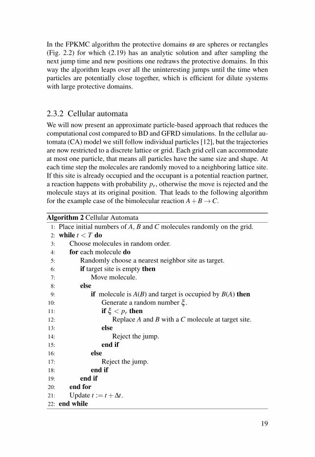
for the example case of the bimolecular reaction A+B →C.

Algorithm 2 Cellular Automata

1: Place initial numbers of A, B and C molecules randomly on the grid.

2: while t < T do3: Choose molecules in random order.

4: for each molecule do5: Randomly choose a nearest neighbor site as target.

6: if target site is empty then7: Move molecule.

8: else9: if molecule is A(B) and target is occupied by B(A) then

10: Generate a random number ξ .

11: if ξ < pr then12: Replace A and B with a C molecule at target site.

13: else14: Reject the jump.

15: end if16: else17: Reject the jump.

18: end if19: end if20: end for21: Update t := t +Δt.22: end while

19

Since molecules can only move in discrete space, this model is computa-

tionally less expensive than the off-lattice simulations in the previous section.

It can be regarded as a coarse version of the so called cellular potts model

[51], where the grid cells, or "pixels", are combined to form cellular com-

ponents (e.g. the membrane, cytosol, nucleus or molecules). The pixels can

then change their state with a probability proportional to the energy cost of the

transformation allowing to model more complex elements and the morpho-

genesis of whole cells.

2.4 Connection between levels

In this section we present how the three models presented above connect to

each other. The microscopic model is the most accurate model we consider

in this thesis for simulations in computational systems biology. Refining the

microscopic level further leads to molecular dynamics simulations which re-

solve space on a much finer scale, so that simulations are restricted to either

few atoms or to short time scales. Attempts to include detailed molecular dy-

namics information such as interaction potentials into the microscopic model

are outlined in [114].

The spatial RDME is a coarse space model where the positions of indi-

vidual particles are no longer resolved and we only keep track of how many

molecules are located inside subdomains of size h at each time step. For a

fine space discretization h, the RDME with particularly derived bimolecular

reaction rates [34, 38, 67, 70] agrees with certain properties of microscopic

Brownian dynamics. In a different limit, it is expected that the RDME con-

verges to the well-mixed CME for infinitely fast diffusion γ0. It has recently

been shown [117] that this holds for the elementary reactions in Section 2.2.2,

but not for more complex reactions such Michaelis-Menten dynamics.

The discretized diffusion equation (2.4) and the RREs (2.2) are the deter-

ministic approximations in the limit of large molecule numbers of the DME

(2.15) and the CME (2.11) respectively [83, 84].

From the macroscopic to the microscopic level the models increase con-

siderably in computational cost and the user needs some prior knowledge of

the system to decide which level of accuracy is necessary for its simulation.

To use the computational power only in the domains or for the species, where

it is needed, hybrid methods have been developed, coupling the macroscopic

and mesoscopic levels [14, 15, 40, 63], the mesoscopic and microscopic levels

[41, 64, 80] and the macroscopic and microscopic levels [42].

20

3. Jump coefficients on unstructured meshes

In this chapter we present how to compute the jump rates in (2.13) for the

RDME (2.17). The jump rates λi j from Vi to a neighboring V j have to be

non-negative

λi j ≥ 0 (3.1)

and we denote by

λi = ∑j

λi j (3.2)

the total propensity to leave voxel Vi.

We first compute the expected number of molecules in each voxel from the

DME (2.15) for one species and then divide by the volume Vi of each voxel

and arrive at

ddt

ci = ∑j=1

Vj

Viλ jic j −λici, i = 1, . . . ,N (3.3)

where ci is the concentration of particles in voxel Vi. If we interpret (3.3) as a

semi-discretized version (2.4) of the diffusion equation (2.3), the discretization

coeffcients Di j of the Laplacian Δ are related to the jump coefficients by

λi j =Vj

ViD ji and λi =−Dii. (3.4)

On a Cartesian grid in d dimensions with grid size h, as used in the software

MesoRD [60], a second-order finite difference (FDM) stencil leads to the jump

rates

λi j =γ0

h2and λi =

2dγ0

h2. (3.5)

Living cells have highly curved membranes. In order to represent these

boundaries without using a very fine Cartesian mesh we will use an unstruc-

tured mesh (meaning triangular or tetrahedral). In [68] a finite volume (FVM)

discretization is used to compute the jump coefficients between the trian-

gles/tetrahedra and we will now present the method introduced in [32] and

implemented in the software URDME [25], where the finite element method

(FEM) is used to compute the jump rates between the dual voxels, see Fig. 2.1.

21

3.1 FEM discretization

The FEM discretization of the diffusion equation (2.3) with linear test and

basis functions is

Mct = Sc, (3.6)

where M is the mass matrix and S the stiffness matrix. After masslumping

in M, the mass matrix is a diagonal matrix with Mii = Vi and we multiply by

the inverse of the lumped matrix to obtain the discretization matrix D = M−1Swith

Di j =γ0

Vi

sin(α +β )2sin(α)sin(β )

(3.7)

in 2D with α and β being the angles opposing the edge between xi and x j, see

Fig. 3.1. A similar formula exists in 3D [131]. If

α +β > π, (3.8)

meaning we have a bad quality mesh with elongated triangles, the off-diagonal

entry Di j is negative, violating (3.1) and the sufficient condition for the discrete

maximum principle. The maximum principle bounds the solution of parabolic

and elliptic PDEs by its boundary values and in particular guarantees the non-

negativity of solutions to the diffusion equation (2.3). To guarantee physical

approximations of (2.3), the discrete solution is supposed to fulfill a discrete

version of the maximum principle. It has been shown in [76] that it is impos-

sible to construct a linear discretization of the Laplacian that is consistent and

fulfills the maximum principle for any quadrilateral mesh.

In the non-negative FEM (nnFEM) approach we therefore relax the consis-

tency condition in order to obtain jump coefficients fulfilling (3.1) by setting

the negative jump rates to zero, as suggested in [32]. Denote the negative

rates by λi j with the corresponding corrected rate λi j, and recompute the total

propensity to leave voxel Vi by ∑ j λi j = λi. This will lead to λi < λi, hence

particles have a higher propensity to leave voxel Vi and we simulate too fast

diffusion [78].

In Papers I and II we address the problem of negative jump coefficients

on unstructured meshes by proposing a method to compute them based on the

first exit time (FET) introduced for particle based simulations in Section 2.3.1.

3.2 The FET approach for mesoscopic jump rates

3.2.1 Local FET

We will first use the FETs locally: the jump rate out of a domain ω is the

inverse of the first exit time. In Paper II we show that in order to obtain the

correct jump rate to leave Vi on a Cartesian mesh, ω has to be chosen as

the circle with radius h around xi, denoted ωi, see Fig. 3.1. The fact that

22

hVj

xixj

∂ωij

Vi

ωi

(a)

α

β xi

xj

Vk

ωk

xk

(b)

Figure 3.1. The voxels Vi around node xi and the exit time domain ωi on a Cartesian

mesh (a) and an unstructured mesh (b). The red edge beween xi and x j in (b) leads to

negative jump coefficients with a FEM discretization, since α +β > π .

Vi ⊂ ωi accounts for the extra time the molecules need to become well-mixed

inside the neighboring V j. One possibility is to solve (2.19) and compute the

expected value of (2.21) to obtain λi, but the expected local exit time e(x) of a

diffusing molecule starting in x also fulfills the Poisson equation [101, 107]

γ0Δe(x) =−1, x ∈ ωi (3.9)

e(x) = 0, x ∈ ∂ωi,

which we can solve and compute

λi =1

e(xi). (3.10)

The jump propensity to a certain neighbor λi j fulfills

λi j = θi jλi, (3.11)

where θi j is the expected splitting probability, which can be computed by

taking the expected value in (2.23), or by computing the harmonic measure

[101, 107]

Δθi j(x) = 0, x ∈ ωi (3.12)

θi j(x) = 1, x ∈ ∂ωi j

θi j(x) = 0, x ∈ Ω\ωi j,

with ωi j being the quarter segment closest to the neighbor x j, see Fig 3.1.

In Paper I we extend this approach to a Cartesian mesh with a rectangular

discretization where

hx = κhy (3.13)

and allow for the particles to jump along the diagonals as a first step towards

an unstructured mesh. We compare the jump coefficients resulting from dis-

cretizations with FDM, FVM, FEM and FET in 2D. The FDM is here the

23

convex combination of two five-point stencils with the combination param-

eter α , which we can choose such that the FDM is equivalent to any of the

other methods. Choosing α such that the FDM agrees with the FET coeffi-

cients leads to a high jump propensity and fewer random numbers need to be

generated. We then determine the boundary segments ωi j such that the FET

approach agrees with FDM.

In Paper II we examine the local first exit time approach on a truly unstruc-

tured mesh. There is no general definition of the exit domain ωi as for the

Cartesian case and as an approximation we choose ωi to be the combination

of the neigboring nodes x j. This domain is too small to produce the correct

exit time (it corresponds to the smaller orange diamond for a Cartesian mesh

(Fig. 3.1)) and hence too fast jump times are sampled which over-represents

short jumps, such that the particles accumulate in the smallest voxel. To cir-

cumvent this shortcoming we instead use the FET times globally, as presented

in the next section.

3.2.2 Global FET

In the global approach (GFET) we instead try to correctly model the time it

takes for a diffusing particle to reach the cell membrane, meaning the domain

boundary ∂Ω. By conditioning on the first step we can show that the expected

time it takes for a molecule to travel from a node xi to the domain boundary

is composed of the time it takes to leave a local environment plus the time it

takes to reach the outer domain from the new position

E(xi) = e(xi)+∑j

θi jE(x j). (3.14)

Here, E(xi) is the global expected time to leave Ω from xi and e(xi) the local

expected time to leave node xi to a neighboring node x j. Reorder (3.14) into

∑j

θi j

e(xi)E(x j)− E(xi)

e(xi)=−1. (3.15)

With (3.10) and (3.11) this becomes

∑j

λi jE(x j)−λiE(xi) =−1, (3.16)

which is a discretization of (3.9) on Ω just as the DME (2.15) is a discretiza-

tion of the diffusion equation (2.3). Thus, the discretization matrix D of the

Laplacian also fulfills the discrete exit time equation (3.16). We will exploit

this fact, by correcting the negative coefficients λi j in such a way that the new

coefficients λi j still fulfill (3.16) in order to model the time to reach the cell

membrane correctly. The algorithm proceeds as follows.

24

Algorithm 3 GFET

1: Compute preliminary rates λi j with a FEM discretization of γ0Δ.

2: Solve γ0ΔE(x) =−1 to obtain discrete global exit times E(xi).3: Find λi j such that

minλi j ∑ j(λi j − λi j)2,

∑ j λi j(E(x j)−E(xi)) =−1,λi j ≥ 0, ∀ j.

4: Recompute λi = ∑ j λi j.

If the original coefficients resulting from a FEM discretization are already

non-negative this algorithm preserves them. Otherwise if λi j < 0 we give up

consistency with the Δ-discretization in favor of non-negative coefficients. The

equality constraint in the minimization problem hereby preserves the expected

first exit time. To show this, assume that the coefficients λi j lead to different

exit times E(xi), then by conditioning on the first step

E(xi) =1

λi+∑

j

λi j

λiE(x j). (3.17)

After rearranging we see that −(1, . . . ,1)t = DE which has a unique solution

(due to the Dirichlet boundary condition), so E = E.

In numerical experiments we further confirm that the GFET approach pre-

serves the global first exit times even for an extremely skewed mesh, see

Fig. 3.2, while the nnFEM results in too fast and the FVM in too slow dif-

fusion.

hy

φ

hx hx (0,0) (1,0)

(1,1) (2,1)

(a) Skewed mesh.

0 0.2 0.4 0.6 0.8 10

0.02

0.04

0.06

0.08

0.1

0.12EnnFEMGFETFVM

(b) ϕ = 3/4π

0 0.2 0.4 0.6 0.8 10

0.01

0.02

0.03

0.04

0.05

0.06

0.07

0.08EnnFEMGFETFVM

(c) ϕ = π/2+0.1

Figure 3.2. (a) Illustration of the mesh with skewness parameter ϕ . In the simulations

we use a finer mesh with nx = ny = 21. (b) & (c) The expected global exit time

for a diffusing molecule starting along the diagonal (red line in (a)) for two ϕ . The

reference line E is computed on an unstructured grid with 105 nodes leading to no

negative edges.

We also examine a simple signaling network where molecules of species Aare created in the center (the cell nucleus) and diffuse through the domain (thecytoplasm) with γ0. Once they reach the boundary (the membrane) they aretransformed into molecules of type B which are degraded, see Table 3.1.

25

/0k1−→ A at x0 = (1,0.5)

Aμ−→ B on ∂Ω

Bk2−→ /0 in Ω

Table 3.1. A simple signaling network with parameters: k1 = 50,k2 = 1,μ = 200,γ0 =0.04.

The steady-state concentration of A depends inversely on the speed of dif-

fusion, while the steady-state concentration of B is unaffected by a change in

the diffusion rate. Simulating this system on the mesh in Fig. 3.3 shows that

the faster nnFEM results in a too low concentration of A at the final time, the

slower FVM over-represents A, and the GFET agrees well with the reference

solution. The concentration of B depends on γ0 only by the time it takes to

reach steady-state.

In 2D, mesh generators are often able to generate meshes fulfilling the re-

quirements for non-negative coefficients, whereas for very simple geometries

(spheres and cubes) in 3D in average 17% of the edges have negative jump

coefficients in our experience and the experiments in Paper II show the same

performance of the methods on realistic three-dimensional meshes.

0 5 10 150

10

20

30

40

50

60

70

80

t

Num

ber

of M

olec

ules

AB

(a) nnFEM

0 5 10 150

10

20

30

40

50

60

70

80

t

Num

ber

of M

olec

ules

AB

(b) GFET

0 5 10 150

50

100

150

t

Num

ber

of M

olec

ules

AB

(c) FVM

Figure 3.3. Average of 50 simulations of the system in Table 3.1 simulated on the

mesh in Fig. 3.2(a) with nx = ny = 21 and ϕ = 34 π until time T = 15. The dotted lines

are the reference solutions calculated on an unstructured grid with 105 nodes and no

negative edges.

26

3.3 Error analysis

3.3.1 Backward error

Above we have presented three methods for computing non-negative jump

coefficients on unstructured meshes: (i) nnFEM, which is no longer a consis-

tent discretization of the Laplacian if (3.8) is fulfilled for any edge; (ii) FVM,

which is only consistent with the Laplacian if the mesh is of Voronoi type

[35, 96]; (iii) GFET, which loses consistency with the Laplacian as nnFEM,

but preserves exit times.

In this section we summarize Paper III, where we perform backward analy-

sis to quantify the error when diffusion is simulated with these methods. The

coefficients resulting from these methods correspond to entries in a perturbed

FEM discretization matrix D with only non-negative off-diagonal elements.

From this perturbed matrix we go back to a diffusion equation and interpret

D as the exact discretization matrix of a perturbed equation, with a space-

dependent diffusion constant γ0(x).

Original equation: ct(x, t) =γ0Δc(x, t), (3.18)

Perturbed equation: ct(x, t) =∇ · (γ0(x)∇c(x, t)), (3.19)

for x ∈ Ω, with homogeneous Neumann boundary conditions ∂c∂n = ∂ c

∂n = 0 for

x ∈ ∂Ω, and initial data c0 = c0 at t = 0. We define the backward error as the

error between the two diffusion coefficients

‖γ0 − γ0‖2∗ :=

1

|Ω|∫

Ω‖γ0 − γ0(x)‖2

2 dΩ. (3.20)

The analysis in Paper III shows that it bounds the forward error, the difference

between the perturbed and unperturbed solutions

‖c(x, t)− c(x, t)‖2L2 ≤Ct‖γ0 − γ0‖∗ (3.21)

for a constant C > 0. The linear growth in t is, however, pessimistic since both

solutions start with c0 and converge towards the same steady state solution, so

there is a bounded maximum error.

Using the Poincaré-Friedrich inequality we can also prove that the error

between the first exit time equations corresponding to (3.18) and (3.19) is

bounded by the backward error

‖E(x)− E(x)‖2L2 ≤C‖γ0 − γ0‖∗, (3.22)

see Theorem 3.5 in Paper III.

3.3.2 Computing γ0

To quantify the error we need to compute the perturbed diffusion coefficient

γ0(x). The lumped mass matrix is the same for both equations, so D = M−1S.

27

The perturbed coefficient γ0(x) then fulfills the FEM discretization formula

Si j =−(∇ψi, γ0(x)∇ψ j). (3.23)

Since we use a linear finite element discretization with linear basis functions

ψi it is only the mean value of γ0(x) on each triangle that contributes to (3.23)

and we assume that γ0(x) is symmetric and constant on each triangle Tk with

mean value γk. In a geometry with ne edges and nt triangles we hence have neconstraints of type (3.23) and 3nt (6nt) degrees of freedom in 2D (3D), so γ0(x)is not uniquely defined. However, (3.21) and (3.22) hold for all γ0(x) fulfilling

(3.23), so we compute the one minimizing (3.20) to obtain the sharpest bound.

Local and global algorithms to compute γ0(x) are presented in Sections 4.2

and 4.3 in Paper III.

3.3.3 Minimal backward error

The backward analysis can be extended by relaxing the constraint (3.23) to

only require that the resulting coefficient is non-negative

0 ≤−(∇ψi, γ0(x)∇ψ j). (3.24)

This allows a larger search space to minimize the backward error (3.20) and we

call this approach the minimal backward error (MBE). The local and global al-

gorithms for minimizing (3.20) to compute the coefficients in MBE and γ0(x)

−0.5 0 0.5−0.5

0

0.5

(a) FVM

-0.5 0 0.5-0.5

0

0.5

(b) GFET

−0.5 0 0.5−0.5

0

0.5

(c) nnFEM

−0.5 0 0.5−0.5

0

0.5

(d) MBE

0.6 < e 0.5 < e ≤ 0.6 0.4 < e ≤ 0.5 0.3 < e ≤ 0.4 0.2 < e ≤ 0.3 0.1 < e ≤ 0.2 0 < e ≤ 0.1 0 = e

(f)

t10-4 10-3 10-2 10-1 100

‖ch−ch‖L2/‖ch‖ L

2

0

0.005

0.01

0.015

0.02

0.025

0.03FVMGFETnnFEMMBEk · t

(g)

‖γ0 − γ0‖∗FVM 0.2729nnFEM 0.1524GFET 0.1356MBE 0.0690

(h)

Figure 3.4. First row: (a)-(d) show the local backwards error e on each triangle for

FVM, GFET, nnFEM and MBE. (f) The bad quality mesh with the edges leading to

negative jump coefficients indicated in red. (g) The relative discrete forward error. (h)

Table with the global backward errors defined in (3.20).

28

are presented in Sections 5.1 and 5.2 in Paper III. We perform numerical ex-

periments on a bad quality mesh in 2D, see Fig. 3.4(f), where the red colored

edges give rise to negative jump coefficients. The first row in Fig. 3.4 shows

the local backward error e = ‖γk − γ0‖2 on each triangle and the table in (h)

shows the normalized sum, the global backward error (3.23). In Fig. 3.4(g)

we see that the time-dependent bound in (3.21) is too pessimistic and that the

backward error correctly ranks the performance of the different methods in the

forward error.

29

4. Macromolecular crowding

In the previous chapters we presented reaction-diffusion models for a dilute

medium, which is a good approximation for test tube experiments resulting in

the dilute diffusion coefficient γ0. Living cells, however, are highly crowded

environments, meaning that a large fraction of the volume is occupied by

macromolecules, while individual species are only present at low concentra-

tions. These molecular obstacles, e.g. proteins, ribosomes, RNA and the cy-

toskeleton occupy up to 40% [89, 113] of the cytoplasm and affect both the

diffusion and reaction rates. The effect is increased on the cell membrane [52],

where attaching actin filaments create barriers for the movement of membrane

bound proteins [74, 82, 94] and inside the mitochondria where around 60% of

the volume is occupied [129].

If the intracellular molecules are modeled as hard spheres the steric re-

pulsions between a diffusing molecule and the numerous "crowders" slow

down diffusion – a hydrodynamic effect. Novel imaging techniques such as

fluorescence-fluctuation analysis [21] have revealed that diffusion can further

become anomalous, meaning that the mean square displacement (MSD) of a

diffusing molecule no longer behaves linearly but sub-linearly in time. For

high crowder densities space decomposes into inhomogeneous subdomains

[59] and becomes a lower dimensional fractal on which diffusion behaves

fundamentally different [9, 61]. Yet, many diffusive phenomena cannot be ex-

plained with steric repulsions alone and more complicated interactions, such

as electrostatic forces or transient binding have to be considered for more ac-

curate models [108, 114], where short-range attraction between obstacles and

moving particles can even increase diffusion [106].

The thermodynamic effect of the excluded volume on the system is that re-

action rates can be both increased and decreased. The impeded diffusion slows

down diffusion-limited reactions, but transition state and rate-limited reactions

and dimerizations are accelerated [29, 58], since the reaction partners reside

in each others vicinity longer, a fact that cells use to increase their efficiency

by clustering and colocalization [44, 98].

Since single-molecule imaging to track individual particles on short time-

scales is still very difficult it is crucial to develop simulation tools that accu-

rately model the intracellular environment, taking crowding effects into ac-

count. In the following sections we present how excluded volume effects due

to steric repulsions are modeled on the three levels of accuracy.

30

4.1 Microscopic model

As mentioned in Section 2.3, particles can be modeled as hard spheres with a

radius r on the microscopic level and excluded volume effects are then inherent

to this model. But the simulations become computationally very expensive

[87], due to the many collisions that have to be modeled in a densely occupied

domain. In [53, 87, 92, 116] microscopic simulations are performed to validate

models for the reaction rates in the crowded environment. The review article

[114] summarizes if and how the different off-lattice microscopic approaches

presented in Section 2.3 account for excluded volume effects.

Another approach is to perform computationally less expensive CA sim-

ulations, to investigate effective reaction rates in the crowded environment

[10, 20, 54, 113, 121]. We will examine the performance of the CA model in

a crowded environment in detail in the next section.

4.1.1 CA and crowding

Generally, the CA model assumes that all molecules have the same size and

shape, but in [28] the effect of differently sized and shaped crowding molecules

(consisting of a combination of cubes) has been studied. The choice of the grid

furthermore influences how strongly the excluded volume effect changes the

reaction rates. In [54] it is shown that the CA model overestimates the crowd-

ing effect on fractal reaction dynamics. The discrepancy is due to the limited

degrees of freedom of motion allowed in the on-lattice models.

In Paper V we investigate this effect more closely by comparing BD sim-

ulations generated with the software Smoldyn [6, 7] to CA simulations on a

Cartesian and on a hexagonal mesh. In a pure diffusion simulation we observe

that the models behave differently than was observed in [54] for the reaction

rates: for occupied volume fractions φ relevant for intracellular simulations,

the BD diffusion is much more obstructed than the lattice-based approaches,

see Fig. 4.1(a).

A possible explanation is that the grid structure orders the molecules (just

like cars on a parking lot), which effectively excludes less space as compared

to when the particles can be placed randomly (imagine finding a parking spot

if the other cars are parked randomly), as illustrated in Fig. 4.2. This makes the

particles more mobile in the CA model than in the BD model. In other words,

it is more probable to choose the free direction out of the restricted number of

directions on a lattice, than the very small angle of possible movement ϕ out

of 2π in BD, see Fig. 4.2(c). The hexagonal mesh here agrees less with the

off-lattice simulation, since it allows for more possible jump directions and

hence even faster diffusion than the Cartesian discretization.

The excluded volume effect on the reaction rates can be modeled by: (i) a

time-dependent diffusion constant k(t), following fractal kinetics [10, 54], or

modified fractal kinetics [113]; or (ii) static corrections, such as a power-law

31

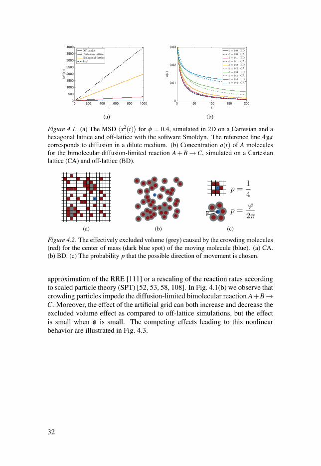
t0 200 400 600 800 1000

〈x2(t)〉

0

500

1000

1500

2000

2500

3000

3500

4000Off-latticeCartesian latticeHexagonal lattice4γ0t

(a)

t0 50 100 150 200

a(t)

0

0.01

0.02

0.03φ = 0.0 : BDφ = 0.0 : CAφ = 0.1 : BDφ = 0.1 : CAφ = 0.2 : BDφ = 0.2 : CAφ = 0.3 : BDφ = 0.3 : CAφ = 0.4 : BDφ = 0.4 : CA

(b)

Figure 4.1. (a) The MSD 〈x2(t)〉 for φ = 0.4, simulated in 2D on a Cartesian and a

hexagonal lattice and off-lattice with the software Smoldyn. The reference line 4γ0tcorresponds to diffusion in a dilute medium. (b) Concentration a(t) of A molecules

for the bimolecular diffusion-limited reaction A+B → C, simulated on a Cartesian

lattice (CA) and off-lattice (BD).

(a) (b)

ϕ

p =1

4

p =ϕ

2π

(c)

Figure 4.2. The effectively excluded volume (grey) caused by the crowding molecules

(red) for the center of mass (dark blue spot) of the moving molecule (blue). (a) CA.

(b) BD. (c) The probability p that the possible direction of movement is chosen.

approximation of the RRE [111] or a rescaling of the reaction rates according

to scaled particle theory (SPT) [52, 53, 58, 108]. In Fig. 4.1(b) we observe that

crowding particles impede the diffusion-limited bimolecular reaction A+B →C. Moreover, the effect of the artificial grid can both increase and decrease the

excluded volume effect as compared to off-lattice simulations, but the effect

is small when φ is small. The competing effects leading to this nonlinear

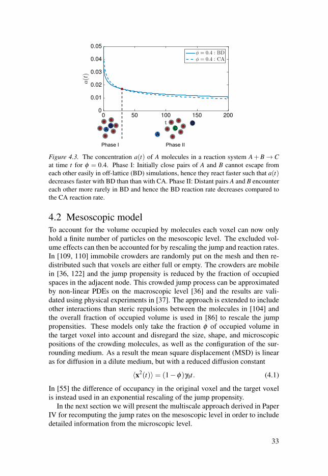
behavior are illustrated in Fig. 4.3.

32

t0 50 100 150 200

a(t)

0

0.01

0.02

0.03

0.04

0.05φ = 0.4 : BDφ = 0.4 : CA

A B C

B

A

Phase I Phase II

Figure 4.3. The concentration a(t) of A molecules in a reaction system A+B → Cat time t for φ = 0.4. Phase I: Initially close pairs of A and B cannot escape from

each other easily in off-lattice (BD) simulations, hence they react faster such that a(t)decreases faster with BD than than with CA. Phase II: Distant pairs A and B encounter

each other more rarely in BD and hence the BD reaction rate decreases compared to

the CA reaction rate.

4.2 Mesoscopic modelTo account for the volume occupied by molecules each voxel can now only

hold a finite number of particles on the mesoscopic level. The excluded vol-

ume effects can then be accounted for by rescaling the jump and reaction rates.

In [109, 110] immobile crowders are randomly put on the mesh and then re-

distributed such that voxels are either full or empty. The crowders are mobile

in [36, 122] and the jump propensity is reduced by the fraction of occupied

spaces in the adjacent node. This crowded jump process can be approximated

by non-linear PDEs on the macroscopic level [36] and the results are vali-

dated using physical experiments in [37]. The approach is extended to include

other interactions than steric repulsions between the molecules in [104] and

the overall fraction of occupied volume is used in [86] to rescale the jump

propensities. These models only take the fraction φ of occupied volume in

the target voxel into account and disregard the size, shape, and microscopic

positions of the crowding molecules, as well as the configuration of the sur-

rounding medium. As a result the mean square displacement (MSD) is linear

as for diffusion in a dilute medium, but with a reduced diffusion constant

〈x2(t)〉= (1−φ)γ0t. (4.1)

In [55] the difference of occupancy in the original voxel and the target voxel

is instead used in an exponential rescaling of the jump propensity.

In the next section we will present the multiscale approach derived in Paper

IV for recomputing the jump rates on the mesoscopic level in order to include

detailed information from the microscopic level.

33

4.2.1 Multiscale approach

In Paper II we showed that the local first exit time from a circle ωi with center

xi and radius h can be used to compute the mesoscopic jump rate λi on a Carte-

sian grid by solving (3.9) and (3.12). We extend this framework to include

macromolecular crowding effects in Paper IV, where the crowding molecules

are represented as stationary holes with reflecting boundary conditions in ωi,

see Fig. 4.4. Since Equation (3.9) models the diffusion of a point particle we

have to add the radius of the spherical diffusing particle to the excluded vol-

ume, see Fig. 4.4(b). In this way, we account for the microscopic positions

and orientations of the crowding molecules, but compute the jump rates on

an overlying Cartesian grid that does no longer resolve the numerous crow-

ders. Consequently the up-scaled stochastic simulations are computationally

cheaper than approaches that microscopically resolve the obstacles during the

jump process. However, we have to numerically solve PDEs of type (3.9) and

(3.12) on each perforated ωi in a pre-computing step, similar to multiscale

methods for solving porous media flow [13, 91]. It is important to mention

that the crowding particles can have any shape, contrary to previous models

where they have to be spherical.

(a)

Crowder Moving molecule Excluded volume

(b)

Figure 4.4. (a) Solution to (3.9) with excluded volume. (b) The excluded volume

consists of the volume occupied by the crowder enlarged by the radius r of the moving

molecule.

In Fig. 4.5 we see that the jump rate depends severely on the size and shape

of the crowding molecules as well as on the size of the diffusing molecule. The

movement of larger particles is more obstructed than that of smaller ones and

small crowding molecules with more reflective surfaces also have a stronger

effect. This agrees with the experimental and theoretical results in [100]. We

furthermore observe that the linear scaling with the occupancy φ underesti-

mates crowding for larger molecules and that the exponential scaling with the

occupancy proposed in [55] is an appropriate model when the diffusing and

crowding particles are similar in size.

Using (3.5), (3.10), and the crowded local first exit times e(xi) we compute

a space-dependent scalar diffusion map

γ(x)|x∈Vi=

h2

2de(xi), (4.2)

34

φ

0 0.1 0.2 0.3 0.4 0.5 0.6

E[λ

i]/E[λ

0,i]

0

0.2

0.4

0.6

0.8

1R = 0.05R = 0.10.02× 0.40.04× 0.81− φ

(a) r = 0.01

φ

0 0.1 0.2 0.3 0.4 0.5 0.6

E[λ

i]/E[λ

0,i]

0

0.2

0.4

0.6

0.8

1R = 0.05R = 0.10.02× 0.40.04× 0.81− φ

(b) r = 0.1

Figure 4.5. The mean value of the mesoscopic jump coefficients in the crowded en-

vironment E[λi] compared to E[λ0,i] = 4 in dilute media for h = 1. Averages are

taken over M = 100 different crowder distributions. The obstacles are either small

spheres (blue)/rectangles (orange) or larger spheres (red)/rectangles (green). The ratio

of width to length is 20 for the rectangles. The spherical moving molecule has radius

r and the spherical crowders have radius R.

to model Fickian diffusion in a crowded environment on the macroscopic level

ct(x, t) = ∇ · (γ(x)∇c(x, t)). (4.3)

We can further use the space-dependent diffusion coefficient γ(x) to compute

space-dependent reaction rates using the Collins-Kimball formula in 3D [19]

(a similar formula exists for 2D)

k(x) =1

h3

4πσγ(x)kr

4πσγ(x)+ kr. (4.4)

In 3D simulations we compute the time until a reaction happens in the sim-

ple reaction network A+B →C. The A-molecule is static in voxel Vi and B is

diffusing with starting position V j. The expected time for the reaction to occur

is

Erj = Ei(x j)+

h2 +4γi ∑m θimEi(xm)

h2ki, (4.5)

where Ei(x j) is the expected time it takes a diffusing molecule starting in V jto reach Vi. We model a local fluctuation in the excluded volume, leading to

fluctuations in the diffusivity, by two different diffusion coefficients γi and γinside Vi and the rest of the domain, respectively. The slower diffusion in Vireduces the reaction rate in this voxel, but it also means that the B molecule

resides in this environment for a longer time. Consequently, the effective re-

action time can be decreased for a certain set of parameters, as compared to a

dilute simulation with γ0 = 1, see Fig. 4.6. This simple model of reaction rates

in combination with diffusion rates in a non-uniformly crowded environment

hence captures the increased throughput, achieved in cells by co-localizing re-

action complexes in a reaction cascade, clustering and compartmentalization

[98].

35

γ

xi xj

γi

(a)

γi

0 0.2 0.4 0.6 0.8 1

Er j/E

r j,0

0

0.5

1

1.5

kr = 1e− 4kr = 1e− 3kr = 5e− 3kr = 1e− 2

(b)

γi

0 0.2 0.4 0.6 0.8 1

Er j/E

r j,0

0

0.5

1

1.5

kr = 1e− 4kr = 1e− 3kr = 5e− 3kr = 1e− 2

(c)

Figure 4.6. (a) Experimental setting where a B molecule starts diffusing in x j =(0.7,0.5,0.5) and reacts with A that is confined to voxel Vi with xi = (0.5,0.5,0.5).Due to an uneven distribution of crowders we assume that the diffusion rates are γiinside Vi and γ (vertical dashed line) in the rest of the domain. The time it takes to re-

act in this crowded environment Erj is compared to that in an uncrowded environment

Erj,0 with γ0 = 1. (b) γ = 0.7. (c) γ = 0.9.

4.3 Macroscopic model

One way of modeling crowding effects on the macroscopic level, is reducing

the diffusion constant [105]. Another model is anomalous diffusion, where the

MSD behaves nonlinear in time

〈x2(t)〉= 2dγ0tα , (4.6)

with α = 1. Often, α < 1 is used to model subdiffusion inside cells. The

anomalous behavior often only becomes apparent when multiple species or

individually-tracked molecules are observed. One can then compare the mean

behavior in time along individual trajectories to ensemble averages, to observe

ergodicity breaking [8, 115], one characteristic of anomalous diffusion. For a

system with two distinct species also non-linear diffusion equations are de-

rived in [86]. Fractional partial differential equation (FPDE) models lead to

a transient anomalous diffusion phase. This corresponds to diffusion with a

time-dependent diffusion coefficient and can model diffusion in an environ-

ment with moving crowders. The internal states model in [11, 97] represents

this time-dependent diffusion coefficient by different internal states in which

the molecules can be and which they can change randomly. As mentioned in

the previous section, we approximate diffusion in a crowded environment on

the mesoscopic level by a space-dependent diffusion coefficient corresponding

to an inhomogeneous distribution of crowding particles. This approach can be

extended to moving crowders by pre-computing statistics for the distribution

of possible diffusion coefficients and then sampling new diffusion coefficients

on the time scale of the movement of the crowding molecules.

36

5. Summary

To understand the gene regulatory networks active inside living cells, math-

ematical models are crucial tools. A large class of models assumes the cells

to be homogeneous in space and hence only includes the chemical reactions.

It has been shown, however, that certain dynamics can only be captured with

space-dependent models, since cells are spatially highly organized.

On the macroscopic level the concentrations of molecules are described by

deterministic partial differential equations, which are a good model for large

molecule numbers. Yet, important species inside cells are often only present

at very low copy numbers and a description by discrete stochastic processes

is instead needed. On the stochastic mesoscopic level space is discretized

into voxels and the state of the system is the number of molecules per voxel.

Molecules can jump in a stochastic process from one voxel to a neighbor-

ing voxel to model diffusion and the voxels are considered small enough, so

that the molecules are well-mixed inside and can react randomly with each

other. The most accurate level considered in this thesis is the microscopic

level, where we follow individual particles along their Brownian trajectories

and reactions happen randomly if molecules are located within a reaction ra-

dius.

This thesis focuses on deriving the jump coefficients on the mesoscopic

level for an unstructured space discretization in such a way, that the correct

diffusion speed is preserved. Unstructured meshes have the advantage of rep-

resenting complicated geometries efficiently, but the disadvantage is that they

might lead to negative jump coefficients when the traditional finite element

method is used. We instead use the first exit time framework, established for

the efficient simulation of Brownian motion, to correctly model the time a

signal starting in the cytosol needs to diffuse to the cell membrane. To an-

alyze different methods guaranteeing non-negative jump coefficients on un-

structured meshes we perform backward analysis and compute new jump co-

efficients, which minimize both the error in diffusion constant and particle

distribution.

The other main topic of this thesis is macromolecular crowding. Inside

living cells molecules occupy a large fraction of the available volume, while

individual species are present at only very low concentrations. This setting

is fundamentally different to that of test tubes, where most biochemical ex-

periments are performed. Since it is difficult to conduct experiments inside

living cells mathematical models are important to understand these excluded

volume effects and how they change the outcome of a reaction network. Exist-

ing reaction-diffusion models are either derived for the dilute case or become

37

computationally intractable in crowded environments. We therefore develop a

multiscale approach that takes the microscopic positions of individual obsta-

cles into account, while still allowing us to perform efficient stochastic sim-

ulations on the mesoscopic level. The model also captures the effect that the

reaction rates can be increased despite the present obstacles.

To conclude, this thesis examines how to compute the jump rates in a dis-

crete stochastic diffusion model for unstructured meshes and a crowded en-

vironment, by using first exit times. The mathematical models in systems

biology and the available algorithms are illustrated in Fig. 5.1, and the areas

to which this thesis contributes are highlighted in blue.

Figure 5.1. A summary of the mathematical models used in computational systems

biology. This thesis includes contributions to the blue areas. In Papers I and II we

compute the jump rates on unstructured meshes via FET. In Paper III we analyze the

error introduced when computing non-negative jump rates on a bad quality mesh. We

present a multiscale approach to include molecular crowding effects into the RDME

framework in Paper IV. In Paper V we compare BD and CA simulations in a crowded

environment and examine the grid artifacts in CA.

Acronyms:BD Brownian dynamics

CA cellular automata

CLE chemical Langevin equation

CME chemical master equation

DE diffusion equation

FET first exit time

FPDE fractional partial differential equation

FPKM first passage time kinetic Monte Carlo

GFRD Green’s function reaction dynamics

LNA linear noise approximation

MLMC multi-level Monte Carlo

PBRD particle based reaction-diffusion

PDE partial differential equation

RDME reaction diffusion master equation

RRE reaction rate equation

SPDE stochastic partial differential equation

SPT scaled particle theory

SSA stochastic simulation algorithm

38

•  •  • 

•  •  •  • 

Figure 5.1. Summary of mathematical models of reaction-diffusion kinetics frequently

used as tools in systems biology.

39

6. Authors contribution

Paper I

The ideas and manuscript were developed in close collaboration between the

two authors. The author of this thesis performed the numerical experiments.

Paper II

The ideas and manuscript were developed in close collaboration between the

two authors. The author of this thesis performed the numerical experiments.

Paper III

The ideas and manuscript were developed in close collaboration between the

co-authors. The author of this thesis performed the mathematical analysis and

the numerical experiments.

Paper IV

The author of this thesis is the sole author of the paper.

Paper V

The author of this thesis developed the ideas and wrote the manuscript. The

numerical experiments were performed by M.E. as part of his Master thesis

supervised by the author of this thesis.

40

7. Summary in Swedish

Celler bygger upp alla levande organismer. De är mycket komplicerade: det

finns många olika organeller som utför olika funktioner, ett cellmembran och

kärnan i djur- och växtceller som innehåller DNA. Deras beteende, om de

växer, delar sig eller specialiserar sig styrs av transkription av gener för pro-

duktion av proteiner. I systembiologi analyseras de komplicerade biokemiska

nätverk av gener med återkoppling och hur de styr t.ex. utvecklingen i ett

embryo som börjar differentiera sig. För att kunna förstå cellernas komplexa

beteende räcker det inte att bara göra biologiska experiment utan vi behöver

också matematiska modeller. Den här avhandlingen handlar om beräkningar

i systembiologi, där vi använder oss av datorer för att lösa de ekvationer

och simulera de processer som de matematiska modellerna ger upphov till.

Speciellt tar vi hänsyn till rumsberoende modeller där molekylerna rör sig

genom diffusion.

I biologiska celler finns det ofta bara ett fåtal molekyler av varje sort och

stora talens lag gäller därför inte och det behövs stokastiska simuleringar. Vi

identifierar tre olika nivåer av modellering. Den makroskopiska modellen an-

tar att molekylerna finns i stora mängder och att en deterministisk beskrivning

är tillräckligt noggrann. Diffusionen är här modellerad genom diffusionsekva-

tionen och reaktionerna genom reaktionstermer. På den mesoskopiska nivån

diskretisar vi rummet i voxlar. Tillståndet hos systemet ges av hur många

molekyler det finns av varje sort i varje voxel. Molekylerna får sedan hoppa

i en diskret hopprocess för att modellera diffusionen och vi antar att en voxel

är tillräckligt liten för att molekylerna ska vara väl blandade inuti och där rea-

gerar de med varandra. Den mest noggranna modellen är på mikroskopisknivå. Här följer vi enskilda molekyler i Brownsk rörelse och de kan reagera

med varandra med en viss sannolikhet när de kommer nära varandra.

I artiklarna I, II och III i avhandlingen undersöker vi hur man kan räkna ut

hoppkoeffcienterna i den mesoskopiska modellen när man diskretiserar rum-

met med ett ostrukturerat nät så att diffusionens hastighet blir korrekt. Ett

problem är att den konventionella metoden som diskretiserar diffusionsek-

vationen med en finit elementmetod kan leda till negativa koefficienter vilka

inte är användbara i en stokastisk process där hoppsannolikheterna måste vara

icke-negativa. Vi använder oss därför av ’first exit time’ som garanterar att

tiden att nå ut till cellmembranet är exakt för en signal som startar inne i cy-

tosolen. I artikel III analyserar vi även felet som uppstår i de olika metoder

som garanterar icke-negativa hoppkoefficienter. I artikel IV undersöker vi ett

fenomen som kallas för makromolekylär trängsel. I celler är upp till 40% av

41

volymen upptagen av molekyler, en situation som är väldigt annorlunda jäm-

fört med provrör varifrån de flesta experimentella resultat kommer. För att

förstå vilken effekt den exkluderade volymen har på såväl reaktioner som dif-

fusion utvecklar vi en multiskalmetod som tar hänsyn till lokaliseringen av de

mikroskopiska trängselmolekylerna medan den fortfarande tillåter oss att göra

simuleringar till låg kostnad på den mesoskopiska nivån. Vi återanvänder re-

sultaten från ansatsen med ’first exit time’ för att beräkna hoppkoefficienter

på ett kartesiskt nät och kan även härleda en makroskopisk ekvation med en

rumsvariabel diffusionskoefficient. Reaktionskonstanter förändras också så

att de tar hänsyn till effekten av exkluderad volym. Storleken och formen på

trängselmolekylerna spelar en viktig roll för hur kraftig diffusionen är, vilket

inte tagits hänsyn till i tidigare modeller. Dessutom visar vi hur trängselef-

fekten kan såväl minska som öka reaktionshastigheten, en effekt som celler

utnyttjar genom att samla reaktionskomplex i en klunga för att öka produk-

tiviteten.

I artikel V jämför vi en kontinuerlig och en diskret mikroskopisk mod-

ells förmåga att noggrant simulera reaktions-diffusionssystem i områden med

varierande täthet av andra molekyler.

42

8. Acknowledgments

Per, thank you very much for being a patient supervisor and for sharing your

curiosity in numerical analysis and computational systems biology with me.

Working with you has been very inspiring and I have learned a lot from you.

I would also like to thank my co-authors Stefan Engblom, Andreas Hellander

and Markus Erkisson and the rest of the computational systems biology group

at Uppsala University for the interesting scientific discussions. Comments

from Sonja Mathias, Andreas Hellander, Fredrik Hellman and Per Lötstedt

helped to improve the summary and were greatly appreciated.

A big thanks to all my colleagues at TDB and the rest of the IT Department,

this thesis would have not been possible without fika! Thank you Behrang, for

all the help, exceeding that of a normal officemate. Hanna, Daniel, Emil,

Fredrik, Kalle and Slobodan, thank you for our outside work activities and for

keeping me fit and skiing.

To my non-science friends: Camilla, Chris, Elizabeth and Zhanna, thank

you for all the hours of talking about real things. And again, thank you Camilla

for being such a great roommate and friend and for introducing me to life in

Sweden.

To my family: Liebe Mama, Papa, Carsten, Oma Maria, Opa Dieter und

Oma Giesela danke für die Unterstützung über all die Jahre, von Erklärstunden

bis zum niemals endenden Nachschub an Schokolade. Danke für alles!

This thesis has been financed by research grants from the Swedish Research

Council 621-2001-3148 and the NIBIB of the NIH under Awards No. R01-

EB014877-01. The content of this thesis is solely the responsibility of the

author and does not necessarily represent the official views of these agen-

cies. Generous travel grants from the Anna Maria Lundins stipendiefond, the

Wallenberg foundation, the Liljevalchs foundation, the Swedish Mathematics

Association, stiftelsen Åforsk and the Gertrud Thelin scholarship made my

travels to summer schools, conferences and other universities possible, which

helped me greatly to learn about systems biology.

43

References

[1] B. Alberts, A. Johnson, J. Lewis, M. Raff, K. Roberts, and P. Walter.

Molecular Biology of the Cell. Garland Science, New York, 5th edition, 2007.

[2] D. F. Anderson. Incorporating postleap checks in tau-leaping. J. Chem. Phys.,128(5), 2008.

[3] D. F. Anderson and D. J. Higham. Multilevel Monte Carlo for Continuous

Time Markov Chains, with Applications in Biochemical Kinetics. SIAMMultiscale Model Simul, 10(1):146–179, 2012.

[4] D. F. Anderson, D. J. Higham, and Y. Sun. Complexity of Multilevel Monte

Carlo Tau-Leaping. SIAM J. Numer. Anal., 52(6):3106–3127, 2014.

[5] D. F. Anderson and T. G. Kurtz. Continuous Time Markov Chain Models for

Chemical Reaction Networks. Des. Anal. Biomol. Circuits, pages 3–42, 2011.

[6] S. S. Andrews, N. J. Addy, R. Brent, and A. P. Arkin. Detailed simulations of

cell biology with Smoldyn 2.1. PLoS Comput. Biol., 6(3), 2010.

[7] S. S. Andrews and D. Bray. Stochastic simulation of chemical reactions with

spatial resolution and single molecule detail. Phys. Biol., 1(3-4):137–151,

2004.

[8] E. Barkai, Y. Garini, and R. Metzler. Strange kinetics of single molecules in

living cells. Phys. Today, 65(8):29–35, 2012.

[9] D. Ben-Avraham and S. Havlin. Diffusion and reactions in fractals anddisordered systems. Cambridge University Press, 2000.

[10] H. Berry. Monte Carlo simulations of enzyme reactions in two dimensions:

fractal kinetics and spatial segregation. Biophys. J., 83(4):1891–1901, 2002.

[11] E. Blanc, S. Engblom, A. Hellander, and P. Lötstedt. Mesoscopic modeling of

stochastic reaction-diffusion kinetics in the subdiffusive regime. Mutliscal.Model. Simul., pages 1–30, to appear 2016.

[12] J. P. Boon, D. David, R. Kapral, and A. Lawniczak. Lattice gas automata for

reactive systems. Phys. Rep., 273(2):55–147, 1996.

[13] D. L. Brown. A Multiscale Method for Porous Microstructures. preprintarXiv:1411.1944, pages 1–29, 2014.

[14] K. Burrage, T. Tian, and P. Burrage. A multi-scaled approach for simulating

chemical reaction systems. Prog. Biophys. Mol. Biol., 85(2-3):217–234, 2004.

[15] Y. Cao, D. T. Gillespie, and L. Petzold. Multiscale stochastic simulation

algorithm with stochastic partial equilibrium assumption for chemically

reacting systems. J. Comput. Phys., 206(2):395–411, 2005.

[16] Y. Cao, D. T. Gillespie, and L. R. Petzold. Efficient step size selection for the

tau-leaping simulation method. J. Chem. Phys., 124(4):044109, 2006.

[17] A. Chatterjee, D. G. Vlachos, and M. A. Katsoulakis. Binomial distribution

based τ-leap accelerated stochastic simulation. J. Chem. Phys., 122(2), 2005.

[18] N. Collier, A.-L. Haji-Ali, F. Nobile, E. von Schwerin, and R. Tempone. A

continuation multilevel Monte Carlo algorithm. BIT Numer. Math.,55(2):399–432, 2014.

44

[19] F. C. Collins and G. E. Kimball. Diffusion-controlled reaction rates. J. ColloidSci., 4(4):425–437, 1949.

[20] D. Dab, A. Lawniczak, J.-P. Boon, and R. Kapral. Cellular-automaton model

for reactive systems. Phys. Rev. Lett., 64(20):2462–2465, 1990.

[21] C. Di Rienzo, V. Piazza, E. Gratton, F. Beltram, and F. Cardarelli. Probing

short-range protein Brownian motion in the cytoplasm of living cells. Nat.Commun., 5:5891, 2014.

[22] M. Doi. Stochastic theory of diffusion-controlled reaction. Journal of PhysicsA: Mathematical and General, 9(9):1479, 1976.

[23] M. Doi. Second quantization representation for classical many-particle

system. J. Phys. A. Math. Gen., 9(9):1465–1477, 2001.

[24] A. Donev, V. V. Bulatov, T. Oppelstrup, G. H. Gilmer, B. Sadigh, and M. H.

Kalos. A First-Passage Kinetic Monte Carlo algorithm for complex

diffusion-reaction systems. J. Comput. Phys., 229(9):3214–3236, 2010.

[25] B. Drawert, S. Engblom, and A. Hellander. URDME: a modular framework

for stochastic simulation of reaction-transport processes in complex

geometries. BMC Syst. Biol., 6(1):76, 2012.

[26] B. Drawert, M. J. Lawson, L. Petzold, and M. Khammash. The diffusive finite

state projection algorithm for efficient simulation of the stochastic

reaction-diffusion master equation. J. Chem. Phys., 132(2010):074101, 2010.

[27] J. Elf and M. Ehrenberg. Spontaneous separation of bi-stable biochemical

systems into spatial domains of opposite phases. Syst. Biol. IEE Proc.,1(2):230–236, 2004.

[28] A. J. Ellery, R. E. Baker, and M. J. Simpson. Calculating the Fickian

diffusivity for a lattice-based random walk with agents and obstacles of

different shapes and sizes. Phys. Biol., 12(6):066010, 2015.

[29] R. J. Ellis. Macromolecular crowding: An important but neglected aspect of

the intracellular environment. Curr. Opin. Struct. Biol., 11(1):114–119, 2001.

[30] S. Engblom. Computing the moments of high dimensional solutions of the

master equation. Appl. Math. Comput., 180(2):498–515, 2006.

[31] S. Engblom. Spectral approximation of solutions to the chemical master

equation. J. Comput. Appl. Math., 229(1):208–221, 2009.

[32] S. Engblom, L. Ferm, A. Hellander, and P. Lötstedt. Simulation of stochastic

reaction-diffusion processes on unstructured meshes. SIAM J. Sci. Comput.,31(3):1774–1797, 2009.

[33] R. Erban, J. S. Chapman, and P. K. Maini. A practical guide to stochastic

simulations of reaction-diffusion processes. arXiv Prepr. arXiv0704.1908,

pages 24–29, 2007.

[34] R. Erban and S. J. Chapman. Stochastic modelling of reaction-diffusion

processes: algorithms for bimolecular reactions. Phys. Biol., 6(4):046001,

2009.

[35] R. Eymard, T. Gallouët, and R. Herbin. A cell-centred finite-volume

approximation for anisotropic diffusion operators on unstructured meshes in

any space dimension. IMA J. Numer. Anal., 26(2):326–353, 2006.

[36] D. Fanelli and A. J. McKane. Diffusion in a crowded environment. Phys. Rev.E - Stat. Nonlinear, Soft Matter Phys., 82(2):1–4, 2010.

45

[37] D. Fanelli, A. J. McKane, G. Pompili, B. Tiribilli, M. Vassalli, and

T. Biancalani. Diffusion of two molecular species in a crowded environment:

theory and experiments. Phys. Biol., 10(4):045008, 2013.

[38] D. Fange, O. G. Berg, P. Sjöberg, and J. Elf. Stochastic reaction-diffusion

kinetics in the microscopic limit. Proc. Natl. Acad. Sci. U. S. A.,107(46):19820–5, 2010.

[39] D. Fange and J. Elf. Noise-induced min phenotypes in E. coli. PLoS Comput.Biol., 2(6):0637–0648, 2006.

[40] L. Ferm, A. Hellander, and P. Lötstedt. An adaptive algorithm for simulation

of stochastic reaction-diffusion processes. J. Comput. Phys., 229(2):343–360,

2010.

[41] M. B. Flegg, S. Hellander, and R. Erban. Convergence of methods for

coupling of microscopic and mesoscopic reaction-diffusion simulations. J.Comput. Phys., 289:1–17, 2015.

[42] B. Franz, M. B. Flegg, S. J. Chapman, and R. Erban. Multiscale

Reaction-Diffusion Algorithms: PDE-Assisted Brownian Dynamics. SIAM J.Appl. Math., 73(3):1224–1247, 2013.

[43] P. L. Freddolino and S. Tavazoie. The dawn of virtual cell biology. Cell,150(2):248–250, 2012.

[44] G. M. Fricke and J. L. Thomas. Receptor aggregation by intermembrane

interactions: A Monte Carlo study. Biophys. Chem., 119(2):205–211, 2006.

[45] M. A Gibson and J. Bruck. Efficient Exact Stochastic Simulation of Chemical

Systems with Many Species and Many Channels. J. Phys. Chem. A,

2:1876–1889, 2000.

[46] M. Giles. Multi-level Monte Carlo path simulation. Oper. Res.,56(3):607–617, 2008.

[47] D. T. Gillespie. A general method for numerically simulating the stochastic

time evolution of coupled chemical reactions. J. Comput. Phys.,22(4):403–434, 1976.

[48] D. T. Gillespie. Exact Stochastic Simulation of couple chemical reactions. J.Phys. Chem., 81(25):2340–2361, 1977.

[49] D. T. Gillespie. Approximate accelerated stochastic simulation of chemically

reacting systems. J. Chem. Phys., 115(4):1716–1733, 2001.

[50] D. T. Gillespie, A. Hellander, and L. R. Petzold. Perspective: Stochastic

algorithms for chemical kinetics. J. Chem. Phys., 138(17), 2013.

[51] F. Graner and J. A. Glazier. Simulation of Biological Cell Sorting Using

Two-Dimensiona Extended Potts Model. Phys. Rev. Lett., 69(13):2013–2016,

1992.

[52] B. Grasberger, A. P. Minton, C. DeLisi, and H. Metzger. Interaction between

proteins localized in membranes. Proc. Natl. Acad. Sci. U. S. A.,83(17):6258–6262, 1986.

[53] R. Grima. Intrinsic biochemical noise in crowded intracellular conditions. J.Chem. Phys., 132(18), 2010.

[54] R. Grima and S. Schnell. A systematic investigation of the rate laws valid in

intracellular environments. Biophys. Chem., 124(1):1–10, 2006.

[55] R. Grima and S. Schnell. A mesoscopic simulation approach for modeling

intracellular reactions. J. Stat. Phys., 128(1-2):139–164, 2007.

46

[56] R. Grima, P. Thomas, and A. V. Straube. How accurate are the nonlinear

chemical Fokker-Planck and chemical Langevin equations? J. Chem. Phys.,135(8), 2011.

[57] C. M. Guldberg and P. Waage. Studies concerning affinity. CM Forhandlinger:Videnskabs-Selskabet i Christiana, 35, 1864.

[58] D. Hall and A. P. Minton. Macromolecular crowding: Qualitative and

semiquantitative successes, quantitative challenges. Biochim. Biophys. Acta -Proteins Proteomics, 1649(2):127–139, 2003.

[59] M. M. K. Hansen, L. H. H. Meijer, E. Spruijt, R. J. M. Maas, M. V.

Rosquelles, J. Groen, H. A. Heus, and W. T. S. Huck. Macromolecular

crowding creates heterogeneous environments of gene expression in picolitre

droplets. Nat. Nanotechnol., 11(October):1–8, 2015.

[60] J. Hattne, D. Fange, and J. Elf. Stochastic reaction-diffusion simulation with

MesoRD. Bioinformatics, 21(12):2923–2924, 2005.

[61] S. Havlin and D. Ben-Avraham. Diffusion in disordered media. Advances inPhysics, 36(6):695–798, 1987.

[62] F. Hayot and C. Jayaprakash. The linear noise approximation for molecular

fluctuations within cells. Phys. Biol., 1(3-4):205–10, 2004.

[63] M. Hegland, A. Hellander, and P. Lötstedt. Sparse grids and hybrid methods

for the chemical master equation. BIT Numer. Math., 48(2):265–283, 2008.

[64] A. Hellander, S. Hellander, and P. Lötstedt. Coupled Mesoscopic and

Microscopic Simulation of Stochastic Reaction-Diffusion Processes in Mixed

Dimensions. Multiscale Model. Simul., 10(2):585–611, 2012.

[65] A. Hellander and P. Lötstedt. Hybrid method for the chemical master equation.

J. Comput. Phys., 227(1):100–122, 2007.

[66] S. Hellander, A. Hellander, and L. Petzold. Reaction-diffusion master equation

in the microscopic limit. Phys. Rev. E - Stat. Nonlinear, Soft Matter Phys.,85(4):1–5, 2012.

[67] S. Hellander, A. Hellander, and L. Petzold. Reaction rates for mesoscopic

reaction-diffusion kinetics. Phys. Rev. E, 91(2), 2015.

[68] I. Hepburn, W. Chen, S. Wils, and E. De Schutter. STEPS: efficient simulation

of stochastic reaction-diffusion models in realistic morphologies. BMC Syst.Biol., 6(1):36, may 2012.

[69] S. A. Isaacson. The reaction-diffusion master equation as an asymptotic

approximation of diffusion to a small target. SIAM J. Appl. Math.,70(1):77–111, 2009.

[70] S. A. Isaacson. A convergent reaction-diffusion master equation. J. Chem.Phys., 139(5), 2013.

[71] T. Jahnke. On reduced models for the chemical master equation. SIAMMultiscale Model Simul, 9(4):1646–1676, 2011.

[72] T. Jahnke and W. Huisinga. Solving the chemical master equation for

monomolecular reaction systems analytically. J. Math. Biol., 54(1):1–26,

2007.

[73] T. Jahnke and W. Huisinga. A dynamical low-rank approach to the chemical

master equation. Bull. Math. Biol., 70(8):2283–2302, 2008.

47

[74] S. Jin and A. S. Verkman. Single particle tracking of complex diffusion in

membranes: Simulation and detection of barrier, raft, and interaction

phenomena. J. Phys. Chem. B, 111(14):3625–3632, 2007.

[75] J. R. Karr, J. C. Sanghvi, D. N. MacKlin, M. V. Gutschow, J. M. Jacobs,

B. Bolival, N. Assad-Garcia, J. I. Glass, and M. W. Covert. A whole-cell

computational model predicts phenotype from genotype. Cell,150(2):389–401, 2012.

[76] E. Keilegavlen, J. M. Nordbotten, and I. Aavatsmark. Sufficient criteria are

necessary for monotone control volume methods. Appl. Math. Lett.,22(8):1178–1180, aug 2009.

[77] R. A. Kerr, T. M. Bartol, B. Kaminsky, M. Dittrich, J.-C. J. Chang, T. J. Baden,

S. B .and Sejnowski, and J. R. Stiles. Fast Monte Carlo Simulation Methods

for Biological Reaction-Diffusion Systems in Solution and on Surfaces. SIAMJ Sci Comput, 30(6):3126, 2008.

[78] E. Kieri. Accurracy aspects of the reaction-diffusion master equation on

unstructured meshes. Technical Report MSc thesis, UPTEC F 11014, Uppsala

University, Uppsala, Sweden, 2011.

[79] D. J. Kiviet, P. Nghe, N. Walker, S. Boulineau, V. Sunderlikova, and S. J. Tans.

Stochasticity of metabolism and growth at the single-cell level. Nature,

514(7522):376–9, 2014.

[80] M. Klann, A. Ganguly, and H. Koeppl. Hybrid spatial Gillespie and particle

tracking simulation. Bioinformatics, 28(18):549–555, 2012.

[81] E. Klipp, W. Liebermeister, C. Wierling, A. Kowald, H. Lehrach, and

R. Herwig. Systems biology. John Wiley & Sons, Weinheim, 2013.

[82] D. Krapf. Chapter five-mechanisms underlying anomalous diffusion in the

plasma membrane. Current topics in membranes, 75:167–207, 2015.

[83] T. G. Kurtz. Solutions of Ordinary Differential Equations as Limits of Pure

Jump Markov Processes. J. Appl. Probab., 7(1):49–58, 1970.

[84] T. G. Kurtz. Strong approximation theorems for density dependent Markov

chains. Stoch. Process. their Appl., 6(3):223–240, 1978.

[85] T. G. Kurtz. Representations of Markov Processes as Multiparameter Time

Changes. Ann. Probab., 8(4):682–715, 1980.

[86] K. A. Landman and A. E. Fernando. Myopic random walkers and exclusion

processes: Single and multispecies. Phys. A Stat. Mech. its Appl.,390(21-22):3742–3753, 2011.

[87] B. Lee, P. R. LeDuc, and R. Schwartz. Stochastic off-lattice modeling of

molecular self-assembly in crowded environments by Green’s function

reaction dynamics. Phys. Rev. E, 78(3):031911, 2008.

[88] C. Lester, C. A. Yates, M. B. Giles, and R. E. Baker. An adaptive multi-level

simulation algorithm for stochastic biological systems. J. Chem. Phys., 142(2),

2015.

[89] K. Luby-Phelps. Cytoarchitecture and physical properties of cytoplasm:

volume, viscosity, diffusion, intracellular surface area. International review ofcytology, 192:189–221, 1999.

[90] A. Mahmutovic, D. Fange, O. G. Berg, and J. Elf. Lost in presumption:

stochastic reactions in spatial models. Nat. Methods, 9(12):1163–1166, 2012.

48

[91] A. Målqvist and D. Peterseim. Localization of elliptic multiscale problems.

Math. Comput., 83(290):2583–2603, 2016.

[92] T.T. Marquez-Lago, A. Leier, and K. Burrage. Anomalous diffusion and

multifractional Brownian motion: simulating molecular crowding and physical

obstacles in systems biology. IET Syst. Biol., 6(4):134, 2012.

[93] H. McAdams and A. Arkin. It’s a noisy business: Genetic regulation at the

nanomolecular scale. Trends Genet., 15(1998):65–69, 1999.

[94] O. Medalia, I. Weber, A. S. Frangakis, D. Nicastro, G. Gerisch, and

W. Baumeister. Macromolecular architecture in eukaryotic cells visualized by

cryoelectron tomography. Science, 298(5596):1209–1213, 2002.

[95] A. Milias-Argeitis, S. Engblom, P. Bauer, and M. Khammash. Stochastic

focusing coupled with negative feedback enables robust regulation in

biochemical reaction networks. J. R. Soc. Interface, 12(113), 2015.

[96] I. D. Mishev. Finite volume methods on Voronoi meshes. Numer. MethodsPartial Differ. Eq., 14(2):193–212, 1998.

[97] M. S. Mommer and D. Lebiedz. Modeling Subdiffusion Using Reaction

Diffusion Systems. SIAM J. Appl. Math., 70:112–132, 2009.

[98] A. Mugler, A. G. Bailey, K. Takahashi, and P. R. ten Wolde. Membrane

clustering and the role of rebinding in biochemical signaling. Biophys. J.,102(5):1069–1078, 2012.

[99] B. Munsky and M. Khammash. The finite state projection algorithm for the

solution of the chemical master equation. J. Chem. Phys., 124(4), 2006.

[100] N. Muramatsu and A. P. Minton. Tracer diffusion of globular proteins in

concentrated protein solutions. Proc. Natl. Acad. Sci. U. S. A.,85(9):2984–2988, 1988.

[101] B. Øksendal. Stochastic differential equations. Springer, Berlin Heidelberg,

2003.

[102] T. Oppelstrup, V. V. Bulatov, A. Donev, M. H. Kalos, G. H. Gilmer, and

B. Sadigh. First-passage kinetic Monte Carlo method. Phys. Rev. E,

80(6):1–14, dec 2009.

[103] J. Paulsson, O. G. Berg, and M. Ehrenberg. Stochastic focusing:

fluctuation-enhanced sensitivity of intracellular regulation. Proc. Natl. Acad.Sci. U. S. A., 97(13):7148–7153, 2000.

[104] C. J. Penington, B. D. Hughes, and K. A. Landman. Building macroscale

models from microscale probabilistic models: A general probabilistic

approach for nonlinear diffusion and multispecies phenomena. Phys. Rev. E,

84(4):041120, 2011.

[105] R. Phillips, J. Kondev, J. Theriot, and H. Garcia. Physical biology of the cell.Garland Science, New York, 2012.

[106] G. G. Putzel, M. Tagliazucchi, and I. Szleifer. Nonmonotonic diffusion of

particles among larger attractive crowding spheres. Phys. Rev. Lett.,113(3):1–5, 2014.

[107] S. Redner. A guide to first-passage processes. Cambridge University Press,

Cambridge, 2001.

[108] D. Ridgway, G. Broderick, A. Lopez-Campistrous, M. Ru’aini, P. Winter,

M. Hamilton, P. Boulanger, A. Kovalenko, and M. J. Ellison. Coarse-grained

49

molecular simulation of diffusion and reaction kinetics in a crowded virtual

cytoplasm. Biophys. J., 94(10):3748–3759, 2008.

[109] E. Roberts, A. Magis, J. O. Ortiz, W. Baumeister, and Z. Luthey-Schulten.

Noise contributions in an inducible genetic switch: a whole-cell simulation

study. PLoS Comput. Biol., 7(3):e1002010, mar 2011.

[110] E. Roberts, J. E. Stone, and Z. Luthey-Schulten. Lattice microbes:

High-performance stochastic simulation method for the reaction-diffusion

master equation. J. Comput. Chem., 34(3):245–255, 2013.

[111] M. A. Savageau. Biochemical systems analysis: a study of function and designin molecular biology. Addison-Wesley, 1976.

[112] M. Schmoluchowski. Versuch einer mathematischen Theorie der

Koagulationskinetik kolloider Lösungen. Zeitschriftf. physik. Chemie,

92:129–168, 1918.

[113] S. Schnell and T. E. Turner. Reaction kinetics in intracellular environments

with macromolecular crowding: Simulations and rate laws. Prog. Biophys.Mol. Biol., 85(2-3):235–260, 2004.

[114] J. Schöneberg, A. Ullrich, and F. Noé. Simulation tools for particle-based

reaction-diffusion dynamics in continuous space. BMC Biophys., 7(1):11,

2014.

[115] J. H. P. Schulz, E. Barkai, and R. Metzler. Aging Renewal Theory and

Application to Random Walks. Phys. Rev. X, 4(1):011028, 2014.

[116] G. R. Smith, L. Xie, B. Lee, and R. Schwartz. Applying Molecular Crowding

Models to Simulations of Virus Capsid Assembly In Vitro. Biophys. J.,106(1):310–320, 2014.

[117] S. Smith and R. Grima. The breakdown of the reaction-diffusion master

equation with non-elementary rates. preprint arXiv:1601.03064, 2016.

[118] J. R. Stiles, D. van Helden, T. M. Bartol, E. E. Salpeter, and M. M. Salpeter.

Miniature endplate current rise times less than 100 microseconds from

improved dual recordings can be modeled with passive acetylcholine diffusion

from a synaptic vesicle. Proc. Natl. Acad. Sci. U. S. A., 93(12):5747–5752,

1996.

[119] P. S. Swain, M. B. Elowitz, and E. D. Siggia. Intrinsic and extrinsic

contributions to stochasticity in gene expression. Proc. Natl. Acad. Sci. U. S.A., 99(20):12795–12800, 2002.

[120] K. Takahashi, S. Tanase-Nicola, and P. R. ten Wolde. Spatio-temporal

correlations can drastically change the response of a MAPK pathway. Proc.Natl. Acad. Sci. U. S. A., 107(6):2473–2478, 2010.

[121] K. Takahashi, S. N. Vel Arjunan, and M. Tomita. Space in systems biology of

signaling pathways - Towards intracellular molecular crowding in silico. FEBSLett., 579(8):1783–1788, 2005.

[122] P. R. Taylor, C. A. Yates, M. J. Simpson, and R. E. Baker. Reconciling

transport models across scales: The role of volume exclusion. Phys. Rev. E,

92(4):040701, 2015.

[123] T. Tian and K. Burrage. Binomial leap methods for simulating stochastic

chemical kinetics. J. Chem. Phys., 121(21):10356–10364, 2004.

[124] M. Tomita, K. Hashimoto, K. Takahashi, T. S. Shimizu, Y. Matsuzaki,

F. Miyoshi, K. Saito, S. Tanida, K. Yugi, J. C. Venter, and C. A. Hutchison.

50

E-CELL: Software environment for whole-cell simulation. Bioinformatics,

15(1):72–84, 1999.

[125] A. M. Turing. The chemical basis of morphogenesis. Philos. Trans. R. Soc.Lond. B. Biol. Sci., 237(641):37–72, 1952.

[126] N.G. van Kampen. Stochastic processes in physics and chemistry. North

Holland, 2007.

[127] J. S. van Zon and P. R. ten Wolde. Green’s-function reaction dynamics: a

particle-based approach for simulating biochemical networks in time and

space. J. Chem. Phys., 123(23):234910, 2005.

[128] J. S. Van Zon and P. R. ten Wolde. Simulating biochemical networks at the

particle level and in time and space: Green’s function reaction dynamics.

Phys. Rev. Lett., 94(12):1–4, 2005.

[129] A. S. Verkman. Solute and macromolecule diffusion in cellular aqueous

compartments. Trends Biochem. Sci., 27(1):27–33, 2002.

[130] J. M. G. Vilar, Hao Y. Kueh, N. Barkai, and S. Leibler. Mechanisms of

noise-resistance in genetic oscillators. Proc. Natl. Acad. Sci. U. S. A.,99(9):5988–5992, 2002.

[131] J. Xu and L. Zikatanov. A Montone Finite Element Scheme for

Convection-Diffusion Equations. Math. Comput., 68(228):1429–1446, 1999.

51

Acta Universitatis UpsaliensisDigital Comprehensive Summaries of Uppsala Dissertationsfrom the Faculty of Science and Technology 1376

Editor: The Dean of the Faculty of Science and Technology

A doctoral dissertation from the Faculty of Science andTechnology, Uppsala University, is usually a summary of anumber of papers. A few copies of the complete dissertationare kept at major Swedish research libraries, while thesummary alone is distributed internationally throughthe series Digital Comprehensive Summaries of UppsalaDissertations from the Faculty of Science and Technology.(Prior to January, 2005, the series was published under thetitle “Comprehensive Summaries of Uppsala Dissertationsfrom the Faculty of Science and Technology”.)

Distribution: publications.uu.seurn:nbn:se:uu:diva-284085

ACTAUNIVERSITATIS

UPSALIENSISUPPSALA

2016