Stochastic (partial) differential equations and Gaussian...
79
Stochastic (partial) differential equations and Gaussian processes Simo Särkkä Aalto University, Finland
Transcript of Stochastic (partial) differential equations and Gaussian...

Stochastic (partial) differential equationsand Gaussian processesSimo SärkkäAalto University, Finland

S(P)DEs and GPsSimo Särkkä
2 / 24
Contents
1 Basic ideas
2 Stochastic differential equations and Gaussian processes
3 Stochastic partial differential equations and Gaussianprocesses
4 Conclusion

S(P)DEs and GPsSimo Särkkä
2 / 24
Contents
1 Basic ideas
2 Stochastic differential equations and Gaussian processes
3 Stochastic partial differential equations and Gaussianprocesses
4 Conclusion

S(P)DEs and GPsSimo Särkkä
2 / 24
Contents
1 Basic ideas
2 Stochastic differential equations and Gaussian processes
3 Stochastic partial differential equations and Gaussianprocesses
4 Conclusion

S(P)DEs and GPsSimo Särkkä
2 / 24
Contents
1 Basic ideas
2 Stochastic differential equations and Gaussian processes
3 Stochastic partial differential equations and Gaussianprocesses
4 Conclusion

S(P)DEs and GPsSimo Särkkä
3 / 24
Contents
1 Basic ideas
2 Stochastic differential equations and Gaussian processes
3 Stochastic partial differential equations and Gaussianprocesses
4 Conclusion

S(P)DEs and GPsSimo Särkkä
4 / 24
Kernel vs. SPDE representations of GPsGP model x ∈ Rd , t ∈ R Equivalent S(P)DE modelSpatial k(x,x′) SPDE model (L is an operator)
L f (x) = w(x)
Temporal k(t , t ′) State-space/SDE model
df(t)dt
= A f(t) + L w(t)
Spatio-temporalk(x, t ; x′, t ′)
Stochastic evolution equation
∂
∂tf(x, t) = Ax f(x, t) + L w(x, t)

S(P)DEs and GPsSimo Särkkä
5 / 24
Why use S(P)DE solvers for GPs?
The O(n3) computational complexity is a challenge.What do we get:
O(n) state-space methods for SDEs/SPDEs.Sparse approximations developed for SPDEs.Reduced rank Fourier/basis function approximations.Path to non-Gaussian processes.
Downsides:We often need to approximate.Mathematics can become messy.

S(P)DEs and GPsSimo Särkkä
6 / 24
Contents
1 Basic ideas
2 Stochastic differential equations and Gaussian processes
3 Stochastic partial differential equations and Gaussianprocesses
4 Conclusion

S(P)DEs and GPsSimo Särkkä
7 / 24
Ornstein-Uhlenbeck process
The mean and covariance functions:
m(x) = 0
k(x , x ′) = σ2 exp(−λ|x − x ′|)
This has a path representation as a stochastic differentialequation (SDE):
df (t)dt
= −λ f (t) + w(t).
where w(t) is a white noise process with x relabeled as t .Ornstein–Uhlenbeck process is a Markov process.What does this actually mean =⇒ white board.

S(P)DEs and GPsSimo Särkkä
8 / 24
Ornstein-Uhlenbeck process (cont.)Consider a Gaussian process regression problem
f (x) ∼ GP(0, σ2 exp(−λ|x − x ′|))
yk = f (xk ) + εk
This is equivalent to the state-space model
df (t)dt
= −λ f (t) + w(t)
yk = f (tk ) + εk
that is, with fk = f (tk ) we have a Gauss-Markov model
fk+1 ∼ p(fk+1 | fk )
yk ∼ p(yk | fk )
Solvable in O(n) time using Kalman filter/smoother.

S(P)DEs and GPsSimo Särkkä
9 / 24
State Space Form of Linear Time-Invariant SDEsConsider a Nth order LTI SDE of the form
dN fdtN + aN−1
dN−1fdtN−1 + · · ·+ a0f = w(t).
If we define f = (f , . . . ,dN−1f/dtN−1), we get a state spacemodel:
dfdt
=
0 1
. . . . . .0 1
−a0 −a1 . . . −aN−1
︸ ︷︷ ︸
A
f +
0...01
︸ ︷︷ ︸
L
w(t)
f (t) =(1 0 · · · 0
)︸ ︷︷ ︸H
f.
The vector process f(t) is Markovian although f (t) isn’t.

S(P)DEs and GPsSimo Särkkä
10 / 24
Spectra of Linear Time-Invariant SDEsBy taking the Fourier transform of the LTI SDE, we canderive the spectral density which has the form:
S(ω) =(constant)
(polynomial in ω2)We can also do this conversion to the other direction:
With certain parameter values, the Matérn has the form:
S(ω) ∝ (λ2 + ω2)−(p+1).
Many non-rational spectral densities can be approximated:
S(ω) = σ2√π
κexp
(−ω
2
4κ
)≈ (const)
N!/0!(4κ)N + · · ·+ ω2N
For the conversion of a rational spectral density to aMarkovian (state-space) model, we can use the spectralfactorization.

S(P)DEs and GPsSimo Särkkä
11 / 24
State-space methods for Gaussian processes
Approximation:
S(ω) ≈ b0 + b1 ω2 + · · ·+ bM ω
2M
a0 + a1 ω2 + · · ·+ aN ω2NLocation
(x) Time(t)
f(x
,t)
The state at time t
Results in a linear stochastic differential equation (SDE)
df(t) = A f(t) dt + L dW
More generally stochastic evolution equations.O(n) GP regression with Kalman filters and smoothers.Parallel block-sparse precision methods −→ O(log n).

S(P)DEs and GPsSimo Särkkä
12 / 24
State-space methods – temporal example
Example (Matérn class 1d)The Matérn class of covariance functions is
k(t , t ′) = σ2 21−ν
Γ(ν)
(√2ν`|t − t ′|
)νKν
(√2ν`|t − t ′|
).
When, e.g., ν = 3/2, we have
df(t) =
(0 1−λ2 −2λ
)f(t) dt +
(0
q1/2
)dW (t),
f (t) =(1 0
)f(t).

S(P)DEs and GPsSimo Särkkä
13 / 24
State-space methods – spatio-temporal example
Example (2D Matérn covariance function)Consider a space-time Matérn covariance function
k(x , t ; x ′, t ′) = σ2 21−ν
Γ(ν)
(√2ν
ρ
l
)νKν(√
2νρ
l
).
where we have ρ =√
(t − t ′)2 + (x − x ′)2, ν = 1 andd = 2.We get the following representation:
df(x , t) =
(0 1
∂2
∂x2 − λ2 −2√λ2 − ∂2
∂x2
)f(x , t) dt+
(01
)dW (x , t).
S(P)DEs and GPsSimo Särkkä
14 / 24
Contents
1 Basic ideas
2 Stochastic differential equations and Gaussian processes
3 Stochastic partial differential equations and Gaussianprocesses
4 Conclusion

S(P)DEs and GPsSimo Särkkä
15 / 24
Basic idea of SPDE inference on GPs [1/2]Consider e.g. the stochastic partial differential equation:
∂2f (x , y)
∂x2 +∂2f (x , y)
∂y2 − λ2 f (x , y) = w(x , y)
Fourier transforming gives the spectral density:
S(ωx , ωy ) ∝(λ2 + ω2
x + ω2y
)−2.
Inverse Fourier transform gives the covariance function:
k(x , y ; x ′, y ′) =
√(x − x ′)2 + (y − y ′)2
2λK1(λ
√(x − x ′)2 + (y − y ′)2)
But this is just the Matérn covariance function.

S(P)DEs and GPsSimo Särkkä
16 / 24
Basic idea of SPDE inference on GPs [2/2]More generally, SPDE for some linear operator L:
L f (x) = w(x)
Now f is a GP with precision and covariance operators:
K−1 = L∗ LK = (L∗ L)−1
Idea: approximate L or L−1 using PDE/ODE methods:1 Finite-differences/FEM methods lead to sparse precision
approximations.2 Fourier/basis-function methods lead to reduced rank
covariance approximations.3 Spectral factorization leads to state-space (Kalman)
methods which are time-recursive (or sparse in precision).

S(P)DEs and GPsSimo Särkkä
17 / 24
Finite-differences/FEM – sparse precision
Basic idea:
∂f (x)
∂x≈ f (x + h)− f (x)
h∂2f (x)
∂x2 ≈ f (x + h)− 2f (x) + f (x − h)
h2
We get an SPDE approximation L ≈ L, where L is sparseThe precision operator approximation is then sparse:
K−1 ≈ LT L = sparse
L need to be approximated as integro-differential operator.Requires formation of a grid, but parallelizes well.

S(P)DEs and GPsSimo Särkkä
18 / 24
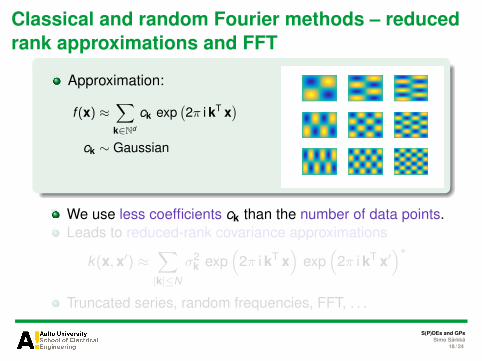
Classical and random Fourier methods – reducedrank approximations and FFT
Approximation:
f (x) ≈∑k∈Nd
ck exp(2π i kT x
)ck ∼ Gaussian
We use less coefficients ck than the number of data points.Leads to reduced-rank covariance approximations
k(x,x′) ≈∑|k|≤N
σ2k exp
(2π i kT x
)exp
(2π i kT x′
)∗Truncated series, random frequencies, FFT, . . .
S(P)DEs and GPsSimo Särkkä
18 / 24
Classical and random Fourier methods – reducedrank approximations and FFT
Approximation:
f (x) ≈∑k∈Nd
ck exp(2π i kT x
)ck ∼ Gaussian
We use less coefficients ck than the number of data points.Leads to reduced-rank covariance approximations
k(x,x′) ≈∑|k|≤N
σ2k exp
(2π i kT x
)exp
(2π i kT x′
)∗Truncated series, random frequencies, FFT, . . .

S(P)DEs and GPsSimo Särkkä
19 / 24
Hilbert-space/Galerkin methods – reduced rankapproximations
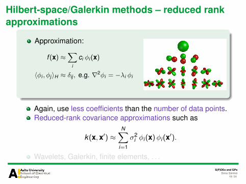
Approximation:
f (x) ≈∑
i
ci φi (x)
〈φi , φj〉H ≈ δij , e.g. ∇2φi = −λi φi
Again, use less coefficients than the number of data points.Reduced-rank covariance approximations such as
k(x,x′) ≈N∑
i=1
σ2i φi(x)φi(x′).
Wavelets, Galerkin, finite elements, . . .

S(P)DEs and GPsSimo Särkkä
19 / 24
Hilbert-space/Galerkin methods – reduced rankapproximations
Approximation:
f (x) ≈∑
i
ci φi (x)
〈φi , φj〉H ≈ δij , e.g. ∇2φi = −λi φi
Again, use less coefficients than the number of data points.Reduced-rank covariance approximations such as
k(x,x′) ≈N∑
i=1
σ2i φi(x)φi(x′).
Wavelets, Galerkin, finite elements, . . .
S(P)DEs and GPsSimo Särkkä
20 / 24
Contents
1 Basic ideas
2 Stochastic differential equations and Gaussian processes
3 Stochastic partial differential equations and Gaussianprocesses
4 Conclusion

S(P)DEs and GPsSimo Särkkä
21 / 24
Back to SPDE representations of GPsGP model x ∈ Rd , t ∈ R Equivalent S(P)DE modelSpatial k(x,x′) SPDE model (L is an operator)
L f (x) = w(x)
Temporal k(t , t ′) State-space/SDE model
df(t)dt
= A f(t) + L w(t)
Spatio-temporalk(x, t ; x′, t ′)
Stochastic evolution equation
∂
∂tf(x, t) = Ax f(x, t) + L w(x, t)

S(P)DEs and GPsSimo Särkkä
22 / 24
What then?
Exchange and map approximations between the fields:Inducing points↔ point-collocation; spectral methods↔Galerkin methods; finite-differences↔ GMRFs;
Non-Gaussian processes: Student’s-t processes,non-linear Itô processes, jump processes, hybridpoint/Gaussian processes.Hierarchical (deep) SPDE models: we stack SPDEs on topof each other – the SPDE just becomes non-linear.Combined first-principles and nonparametric models –latent force models (LFM), also non-linear andnon-Gaussian LFMs.Inverse problems – operators in the measurement model.

S(P)DEs and GPsSimo Särkkä
23 / 24
Summary
Gaussian processes (GPs) are nice, but the computationalscaling is bad.GPs have representations as solutions to SPDEs.In temporal models we can use Kalman/Bayesian filtersand smoothers.SPDE methods can be used to speed up GP inference.New paths towards non-linear GP models.Work nicely in latent force models.

S(P)DEs and GPsSimo Särkkä
24 / 24
Useful references
N. Wiener (1950). Extrapolation, Interpolation and Smoothing ofStationary Time Series with Engineering Applications. John Wiley &Sons, Inc.
R. L. Stratonovich (1963). Topics in the Theory of Random Noise.Gordon and Breach.
J. Hartikainen and S. Särkkä (2010). Kalman Filtering and SmoothingSolutions to Temporal Gaussian Process Regression Models. Proc.MLSP.
S. Särkkä, A. Solin, and J. Hartikainen (2013). Spatio-TemporalLearning via Infinite-Dimensional Bayesian Filtering and Smoothing.IEEE Sig.Proc.Mag., 30(5):51–61.
S. Särkkä (2013). Bayesian Filtering and Smoothing. CambridgeUniversity Press.
S. Särkkä and A. Solin (2017, to appear) Applied StochasticDifferential Equations. Cambridge University Press.


![Stochastic Differential Dynamic Logic for …3 Stochastic Differential Equations We consider stochastic differential equations [Øks07, KP10] to describe stochastic continuous system](https://static.fdocuments.in/doc/165x107/5f397c2e99ca7b6adc05f296/stochastic-differential-dynamic-logic-for-3-stochastic-differential-equations-we.jpg)