arX

iv:1

709.

0732

8v1

[ph

ysic

s.ao

-ph]

21

Sep

2017

Tellus 000, 000–000 (0000) Printed 22 September 2017 (Tellus LATEX style file v2.2)

Stochastic parameterization identification using

ensemble Kalman filtering combined with

expectation-maximization and Newton-Raphson

maximum likelihood methods

Manuel Pulido1, Pierre Tandeo2, Marc Bocquet3, Alberto Carrassi4, and Magdalena Lucini5

1Department of Physics, FaCENA, Universidad Nacional del Nordeste, Corrientes, and IFAECI, CNRS-CONICET, Buenos Aires, Argentina⋆

2Institut Mines-Telecom Atlantique, UMR CNRS 6285 Lab-STICC, Brest, France

3CEREA, joint laboratory Ecole des Ponts ParisTech and EDF R&D, Universite Paris-Est, Champs-sur-Marne, France

4Nansen Environmental and Remote Sensing Center, Bergen, Norway

5Department of Mathematics, FaCENA, Universidad Nacional del Nordeste and CONICET, Corrientes, Argentina

(Manuscript received xx xxxx xx; in final form xx xxxx xx)

A B S T R A C T

For modelling geophysical systems, large-scale processes are described through a set of coarse-grained

dynamical equations while small-scale processes are represented via parameterizations. This work pro-

poses a method for identifying the best possible stochastic parameterization from noisy data. State-the-art

sequential estimation methods such as Kalman and particle filters do not achieve this goal succesfully be-

cause both suffer from the collapse of the parameter posterior distribution. To overcome this intrinsic limi-

tation, we propose two statistical learning methods. They are based on the combination of two methodolo-

gies: the maximization of the likelihood via Expectation-Maximization (EM) and Newton-Raphson (NR)

algorithms which are mainly applied in the statistic and machine learning communities, and the ensemble

Kalman filter (EnKF). The methods are derived using a Bayesian approach for a hidden Markov model.

They are applied to infer deterministic and stochastic physical parameters from noisy observations in

coarse-grained dynamical models. Numerical experiments are conducted using the Lorenz-96 dynamical

system with one and two scales as a proof-of-concept. The imperfect coarse-grained model is modelled

through a one-scale Lorenz-96 system in which a stochastic parameterization is incorpored to represent

the small-scale dynamics. The algorithms are able to identify an optimal stochastic parameterization

with a good accuracy under moderate observational noise. The proposed EnKF-EM and EnKF-NR are

promising statistical learning methods for developing stochastic parameterizations in high-dimensional

geophysical models.

Keywords: parameter estimation, model error estimation, stochastic parameterization

1. Introduction

The statistical combination of observations of a dynamical

model with a priori information of physical laws allows the

estimation of the full state of the model even when it is only

⋆ Corresponding author.

e-mail: pulido@unne.edu.ar

partially observed. This is the main aim of data assimilation

(Kalnay, 2002). One common challenge of evolving multi-scale

systems in applications ranging from meteorology, oceanogra-

phy, hydrology and space physics to biochemistry and biolog-

ical systems is the presence of parameters that do not rely on

known physical constants so that their values are unknown and

unconstrained. Data assimilation techniques can also be for-

c© 0000 Tellus

2

mulated to estimate these model parameters from observations

(Jazwinski, 1970; Wikle and Berliner, 2007).

There are several multi-scale physical systems which are

modelled through coarse-grained equations. The most paradig-

matic cases being climate models (Stensrud, 2009), large-eddy

simulations of turbulent flows (Mason and Thomson, 1992),

and electron fluxes in the radiation belts (Kondrashov et al.,

2011). These imperfect models need to include subgrid-scale

effects through physical parameterizations (Nicolis, 2004). In

the last years, stochastic physical parameterizations have been

incorporated in weather forecast and climate models (Palmer,

2001; Shutts, 2015; Christensen et al., 2015). They are called

stochastic parameterizations because they represent stochasti-

cally a process that is not explicitly resolved in the model, even

when the unresolved process may not be itself stochastic. The

forecast skill of ensemble forecast systems has been shown to

improve with these stochastic parameterizations (Ibid.). Deter-

ministic integrations with models that include these parameter-

izations have also been shown to improve climate features (see

e.g. Lott et al. 2012). In general, stochastic parameterizations

are expected to improve coarse-grained models of multi-scale

physical systems (Katsoulakis et al., 2003; Majda and Gersh-

gorin, 2011). However, the functional form of the schemes and

their parameters, which represents small-scale effects, are un-

known and must be inferred from observations. The develop-

ment of automatic statistical learning techniques to identify an

optimal stochastic parameterization and estimate its parameters

is, therefore, highly desirable.

One standard methodology to estimate physical model pa-

rameters from observations in data assimilation techniques,

such as the traditional Kalman filter, is to augment the state

space with the parameters (Jazwinski, 1970). This methodol-

ogy has also been implemented in the ensemble-based Kalman

filter (see e.g. Anderson 2001). The parameters are constrained

through their correlations with the observed variables.

The collapse of the parameter posterior distribution found in

both ensemble Kalman filters (Delsole and Yang, 2010; Ruiz

et al., 2013a;b; Santitissadeekorn and Jones, 2015) and parti-

cle filters (West and Liu, 2001) is a major contention point

when one is interested in estimating stochastic parameters of

nonlinear dynamical models. Hereinafter, we refer as stochas-

tic parameters to those that define the covariance of a Gaussian

stochastic process (Delsole and Yang, 2010). In other words, the

sequential filters are, in principle, able to estimate deterministic

physical parameters, the mean of the parameter posterior distri-

bution, through the augmented state-space procedure, but they

are unable to estimate stochastic parameters of the model, be-

cause of the collapse of the corresponding posterior distribution.

Using the Kalman filter with the augmentation method, Delsole

and Yang (2010) proved analytically the collapse of the param-

eter covariance in a first-order autoregressive model. They pro-

posed a generalized maximum likelihood estimation using an

approximate sequential method to estimate stochastic param-

eters. Carrassi and Vannitsem (2011) derived the evolution of

the augmented error covariance in the extended Kalman filter

using a quadratic in time approximation that mitigates the col-

lapse of the parameter error covariance. Santitissadeekorn and

Jones (2015) proposed a particle filter blended with an ensemble

Kalman filter and use a random walk model for the parameters.

This technique was able to estimate stochastic parameters in the

first-order autoregressive model, but a tunable parameter in the

random walk model needs to be introduced.

The Expectation-Maximization (EM) algorithm (Dempster

et al., 1977; Bishop, 2006) is a widely used methodology to

maximize the likelihood function in a broad spectrum of ap-

plications. One of the advantages of the EM algorithm is that

its implementation is rather straigthforward. Wu (1983) showed

that if the likelihood is smooth and unimodal, the EM algorithm

converges to the unique maximum likelihood estimate. Accel-

erations of the EM algorithm have been proposed for its use

in machine learning (Neal and Hinton, 1999). Recently, it was

used in an application with a highly nonlinear observation op-

erator (Tandeo et al., 2015). The EM algorithm was able to es-

timate subgrid-scale parameters with good accuracy while stan-

dard ensemble Kalman filter techniques failed. It has also been

applied to the Lorenz-63 system to estimate model error covari-

ance (Dreano et al., 2017).

In this work, we combine for stochastic parameterization

identification these two independent methodologies: the ensem-

ble Kalman filter (Evensen, 1994; 2003) for the state-estimate

with maximum likelihood estimators, the EM (Dempster et al.,

1977; Bishop, 2006) and the Newton-Raphson (NR) algorithms

(Cappe et al., 2005). The derivation of the technique is ex-

plained in detail and simple terms so that readers that are

not from those communities can understand the basis of the

methodologies, how they can be combined, and hopefully fore-

see potential applications in other geophysical systems. The

learning statistical techniques are suitable to infer the functional

form and the parameter values of stochastic parameterizations

in chaotic spatio-temporal dynamical systems. They are eval-

STOCHASTIC PARAMETERIZATION IDENTIFICATION USING MAXIMUM LIKELIHOOD METHODS

3

uated here on a two-scale spatially extended chaotic dynam-

ical system (Lorenz, 1996) to estimate deterministic physical

parameters, together with additive and multiplicative stochastic

parameters. Pulido et al. (2016) evaluated methods based on the

EnKF alone to estimate subgrid-scale parameters in a two-scale

system: they showed that an offline estimation method is able to

recover the functional form of the subgrid-scale parameteriza-

tion, but none of the methods was able to estimate the stochastic

component of the subgrid-scale effects. In the present work, the

results show that the NR and EM techniques are able to uncover

the functional form of the subgrid-scale parameterization while

succesfully determining the stochastic parameters of the repre-

sentation of subgrid-scale effects.

This work is organized as follows. Section 2 briefly intro-

duces the EM algorithm and derives the marginal likelihood of

the data using a Bayesian perspective. The implementation of

the EM and NR likehood maximization algorithms in the con-

text of data assimilation using the ensemble Kalman filter is

also discussed. Section 3 describes the experiments which are

based on the one- and two-scale Lorenz-96 systems. The former

includes simple deterministic and stochastic parameterizations

to represent the effects of the smaller scale to mimic the two-

scale Lorenz-96 system. Section 4 focuses on the results: Sec-

tion 4.1 discusses the experiments for the estimation of model

noise. Section 4.2 shows the results of the estimation of deter-

ministic and stochastic parameters in a perfect-model scenario.

Section 4.3 shows the estimation experiments for an imperfect

model. The conclusions are drawn in Section 5.

2. Methodology

2.1. Hidden Markov model

A hidden Markov model is defined by a stochastic nonlinear

dynamical model M that evolves in time the hidden variables

xk−1 ∈ RN , according to

xk = MΩ(xk−1) + ηk, (1)

where k stands for the time index. The dynamical model M de-

pends on a set of deterministic and stochastic physical parame-

ters denoted by Ω. We assume an additive random model error,

ηk, with covariance matrix Qk = E(

ηkηTk

)

. The notation E ()

stands for the expectation operator, E [f(x)] ≡∫

f(x)p(x)dx

with p being the probability density function of the underlying

process X .

The observations at time k, yk ∈ RM , are related to the hid-

den variables through the observational operator H,

yk = H(xk) + ǫk, (2)

where ǫk is an additive random observation error with observa-

tion error covariance matrix Rk = E(

ǫkǫTk

)

.

Our estimation problem: Given a set of observation vectors

distributed in time, yk, k = 1, . . . ,K, a nonlinear stochastic

dynamical model, M, and a nonlinear observation operator,

H, we want to estimate the initial prior distribution p(x0), the

observation error covariance Rk , the model error covariance

Qk, and deterministic and stochastic physical parameters Ω of

M.

Since the EM literature also uses the term parameter for the

covariances, we need to distinguish them from deterministic

and stochastic model parameters in this work. We refer to the

parameters of a subgrid-scale parameterization (in the physi-

cal model) as physical parameters, including deterministic and

stochastic ones. While the parameters of the likelihood func-

tion are referred to as statistical parameters. These include the

deterministic and stochastic physical parameters, as well as the

initial prior distribution, the observation error covariance and

the model error covariance.

The estimation method we derive is based on maximum

likelihood estimation. Given a set of independent and identi-

cally distributed (iid) observations from a probability density

function represented by p(y1:K |θ), we seek to maximize the

likelihood function L(y1:K ;θ) as a function of θ. We denote

y1, · · · ,yK by y1:K and the set of statistical parameters to

be estimated by θ: the deterministic and stochastic physical pa-

rameters Ω of the dynamical model M as well as observation

error covariances Rk, model error covariances Qk and the ini-

tial prior distribution p(x0). In practical applications, the statis-

tical moments Rk, Qk and P0 are usually poorly constrained. It

may thus be convenient to estimate them jointly with the phys-

ical parameters. The dynamical model is assumed to be nonlin-

ear and to include stochastic processes represented by some of

the physical parameters in Ω.

The estimation technique used in this work is a batch method:

a set of observations taken along a time interval is used to esti-

mate the model state trajectory that is closest to them, consider-

ing measurement and model errors with a least-square criterion

to be established below. The simultaneous use of observations

distributed in time is essential to capture the interplay of the sev-

4

eral statistical parameters and physical stochastic parameters in-

cluded in the estimation problem. The required minimal length

K for the observation window is evaluated in the numerical ex-

periments. The estimation technique may be applied in suces-

sive K-windows. For stochastic parameterizations in which the

parameters are sensitive to processes of different time scales, a

batch method may also be required to capture the sensitivity to

slow processes.

2.2. Expectation-maximization algorithm

The EM algorithm maximizes the log-likelihood of observa-

tions as a function of the statistical parameters θ in the presence

of a hidden state x0:K1,

l(θ) = lnL(y1:K ;θ) = ln

∫

p(x0:K,y1:K ;θ)dx0:K. (3)

An analytic form for the log-likelihood function, (3), can be

obtained only in a few ideal cases. Furthermore, the numeri-

cal evaluation of (3) may involve high-dimensional integration

of the complete likelihood (integrand of (3)). Given an initial

guess of the statistical parameters θ, the EM algorithm max-

imizes the log-likelihood of observations as a function of the

statistical parameters in successive iterations without the need

to evaluate the complete likelihood.

2.2..1. The principles

Let us introduce in the integral (3) an arbitrary probability

density function of the hidden state, q(x0:K),

l(θ) = ln

∫

q(x0:K)p(x0:K ,y1:K ;θ)

q(x0:K)dx0:K . (4)

We assume that the support of q(x0:K) contains that of

p(x0:K,y1:K ;θ). In particular, q(x0:K) may be thought as a

function of a set of fixed statistical parameters θ′, q(x0:K ;θ′).

Using Jensen inequality a lower bound for the log-likelihood is

obtained,

l(θ) >

∫

q(x0:K) ln

(

p(x0:K ,y1:K ;θ)

q(x0:K)

)

dx0:K ≡ Q(q, θ)

(5)

If we choose q(x0:K) = p(x0:K|y1:K ;θ′), the equality is

satisfied in (5), therefore p(x0:K |y1:K ;θ′) is an upper bound to

Q and so it is the q function that maximises Q(q,θ).

1 We use the notation “;”, p(y1:K ;θ) instead of conditioning “|” to

emphasize that θ is not a random variable but a parameter. NR maxi-

mization and EM are point estimation methods so that θ is indeed as-

sumed to be a parameter (Cappe et al., 2005).

From (5) we see that if we maximize Q(q,θ) over θ, we find

a lower bound for l(θ). The idea of the EM algorithm is to first

find the probability density function q that maximizes Q, the

conditional probability of the hidden state given the observa-

tions, and then to determine the parameter θ that maximizes Q.

Hence, the EM algorithm encompasses the following steps:

Expectation: Determine the distribution q that maximizes Q.

This function is easily shown to be q∗ = p(x0:K |y1:K ;θ′) (see

(5); Neal and Hinton 1999). The function q∗ is the conditional

probability of the hidden state given the observations. In prac-

tice, this is obtained by evaluating the conditional probability at

θ′.

Maximization: Determine the statistical parameters θ∗ that

maximize Q(q∗,θ) over θ. The new estimation of the statisti-

cal parameters is denoted by θ∗ while the (fixed) previous es-

timation by θ′. The expectation step is a function of these old

statistical parameters θ′. The part of function Q to maximize is

given by

∫

p(x0:K|y1:K ;θ′) ln (p(x0:K ,y1:K ;θ)) dx0:K ≡

E [ln (p(x0:K ,y1:K ;θ)) |y1:K ] . (6)

where we use the notation E (f(x)|y) ≡∫

f(x)p(x|y)dx

(Jazwinski, 1970). While the function that we want to maximize

is the log-likelihood, the intermediate function (6) of the EM al-

gorithm to maximize is the expectation of the joint distribution

conditioned to the observations.

2.2..2. Expectation-maximization for a hidden Markov model

The joint distribution of a hidden Markov model using the

definition of the conditional probability distribution reads

p(x0:K ,y1:K) = p(x0:K)p(y1:K |x0:K). (7)

The model state probability density function can be expressed as

a product of the transition density from tk to tk+1 using the defi-

nition of the conditional probability distribution and the Markov

property,

p(x0:K) = p(x0)K∏

k=1

p(xk|xk−1). (8)

The observations are mutually independent and are conditioned

on the current state (see (2)) so that

p(y1:K |x0:K) =

K∏

k=1

p(yk|xk). (9)

STOCHASTIC PARAMETERIZATION IDENTIFICATION USING MAXIMUM LIKELIHOOD METHODS

5

Then, replacing (8) and (9) in (7) yields

p(x0:K ,y1:K) = p(x0)

K∏

k=1

p(xk|xk−1)p(yk|xk). (10)

If we now assume a Gaussian hidden Markov model, and that

the covariances Rk and Qk are constant in time, the logarithm

of the joint distribution (10) is then given by

ln(p(x0:K ,y1:K)) = −(M +N)

2ln(2π)−

1

2ln |P0| −

1

2(x0 − x0)

TP

−10 (x0 − x0)−

K

2ln |Q|

−1

2

K∑

k=1

(xk −M (xk−1))TQ

−1(xk −M (xk−1))−K

2ln |R| −

1

2

K∑

k=1

(yk −H (xk))TR

−1(yk −H (xk)).

(11)

The Markov hypothesis implies that model error is not cor-

related in time. Otherwise, we would have cross terms in the

model error summation of (11). The assumption of a Gaussian

hidden Markov model is central to derive a closed form for the

statistical parameters that maximize the intermediate function.

However, the dynamical model and observation operator may

have nonlinear dependencies so that the Gaussian assumption

is not strictly held. We therefore consider an iterative method in

which each step is an approximation. In general, the method will

converge through sucessive approximations. For severe nonlin-

ear dependencies in the dynamical model, the existence of a

single maximum in the log-likelihood is not guaranteed. In that

case, the EM algorithm may converge to a local maximum.

We consider (11) as a function of the statistical parameters in

this Gaussian state-space model. As mentioned, the statistical

parameters, which are in general denoted by θ, are x0, P0, Q,

R, and the physical parameters from M. In this way, the log-

likelihood function is written as

l(θ) = lnL(θ) = ln(p(x0:K ,y1:K ;θ)) (12)

In this Gaussian state-space model, the maximum of the inter-

mediate function in the EM algorithm, (6), may be determined

analytically from

0 = ∇θE [ln (p(x0:K,y1:K ;θ)) |y1:K ]

=

∫

p(x0:K|y1:K ;θ′)∇θ ln(p(x0:K,y1:K ;θ)) dx0:K

= E[

∇θ ln (p(x0:K ,y1:K ; θ)) |y1:K

]

(13)

Note that θ′ is fixed in (13). We only need to find the critical

values of the statistical parameters Q and R. The physical pa-

rameters are appended to the state, so that their model error is

included in Q. The x0, P0 are at the initial time so that they

are obtained as an output of the smoother which gives a Gaus-

sian approximation of p(xk|y1:K) with k = 0, · · · ,K. The

smoother equations are shown in the Appendix.

Differentiating (11) with respect to Q and R and applying the

expectation conditioned to the observations, we can determine

the root of the condition, (13), which gives the maximum of the

intermediate function. The value of the model error covariance,

solution of (13), is

Q =1

K

K∑

k=1

E(

[xk −M (xk−1)] [xk −M (xk−1)]T∣

∣

∣y1:K

)

.

(14)

In the case of the observation error covariance, the solution is

R =1

K

K∑

k=1

E(

[yk −H (xk)] [yk −H (xk)]T∣

∣

∣y1:K

)

.

(15)

Therefore we can summarize the EM algorithm for a hidden

Markov model as:

Expectation: The required set of expectations given the

observations must be evaluated at θi, i being the itera-

tion number, specifically, E (xk|y1:K), E(

xkxTk

∣

∣y1:K

)

, etc.

The outputs of a classical smoother are indeed E (xk|y1:K),

E(

(xk − E (xk|y1:K))(xk − E (xk|y1:K))T∣

∣y1:K

)

which

fully characterize p(xk|y1:K) in the Gaussian case. Hence, this

expectation step involves the application of a foward filter and

a backward smoother.

Maximization: Since we assume Gaussian distributions, the

optimal value of θi+1 can be determined analytically, which

in our model are Q and R, as derived in (14) and (15). These

equations are evaluated using the expectations determined in the

Expectation step.

The basic steps of this EM algorithm are depicted in Fig.

1a. In this work, we use an ensemble-based Gaussian filter,

6

the ensemble transform Kalman filter (Hunt et al., 2007) and

the Rauch-Tung-Striebel smoother (Cosme et al., 2012; Raanes,

2016)2. A short description of these methods is given in the

Appendix. The empirical expectations are determined using the

smoothed ensemble member states at tk, xsm(tk). For instance,

E(

xkxTk

∣

∣

∣y1:K

)

=1

Ne

Ne∑

m=1

xsm(tk)x

sm(tk)

T, (16)

where Ne is the number of ensemble members. Then, using

these empiral expectations R and/or Q are computed from (14)

and/or (15).

The EM algorithm applied to a linear Gaussian state space

model using the Kalman filter was first proposed by Shumway

and Stoffer (1982). Its approximation using an ensemble of

draws (Monte Carlo EM) was proposed in Wei and Tanner

(1990). It was later generalized with the extended Kalman filter

and Gaussian kernels by Ghahramani and Roweis (1999). The

use of the EnKF and the ensemble Kalman smoother permits the

extension of the EM algorithm to nonlinear high-dimensional

dynamical models and nonlinear observation operators.

2.3. Maximum likelihood estimation via

Newton-Raphson

The EM algorithm is highly versatile and can be readily im-

plemented. However, it requires the optimal value in the max-

imization step to be computed analytically which limits the

range of its applications. If physical parameters of a nonlinear

model need to be estimated, an analytical expression for the op-

timal statistical parameter values may not be available. Another

approach to find an estimate of the statistical parameters con-

sists in maximizing an approximation of the likelihood func-

tion l(θ) with respect to the parameters, (3). This maximization

may be conducted using standard optimization methods (Cappe

et al., 2005).

Following Carrassi et al. (2017), the observation probability

density function can be decomposed into the product

p(y1:K ;θ) =K∏

k=1

p(yk|y1:k−1;θ), (17)

2 In principle what is required in (6) is p(x0:K |y1:K) so that a fixed-

interval smoother needs to be applied. However, it has been shown

by Raanes that the Rauch-Tung-Striebel smoother and the ensemble

Kalman smoother, a fixed-interval smoother, are equivalent even in the

nonlinear, non-Gaussian case.

with the convention y1:0 = ∅. In the case of sequential ap-

plication of NR maximization in successive K-windows, the a

priori probability distribution p(x0) can be taken from the pre-

vious estimation. For such a case, we leave implicit the con-

ditioning in (17) on all the past observations, p(y1:K ;θ) =

p(y1:K |y:0;θ), y:0 = y0,y−1,y−2, · · · which is called

contextual evidence in Carrassi et al. (2017). The times of the

evidencing window, 1 : K, required for the estimation are the

only ones that are kept explicit in (17).

Replacing (17) in (3) yields

l(θ) =K∑

k=1

ln p(yk|y1:k−1;θ)

=

K∑

k=1

ln

(∫

p(yk|xk)p(xk|y1:k−1;θ)dxk

)

. (18)

If we assume Gaussian distributions and linear dynamical and

observational models, the integrand in (18) is exactly the analy-

sis distribution given by a Kalman filter (Carrassi et al., 2017).

The likelihood of the observations conditioned on the state at

each time is then given by

p(yk|xk) = [(2π)M/2|R|1/2]−1

exp

[

−1

2(yk −H(xk))

TR

−1(yk −H(xk))

]

,

(19)

and the prior forecast distribution,

p(xk|y1:k−1;θ) = [(2π)N/2|Pfk |

1/2]−1

exp

[

−1

2(xk − x

fk)

T(Pfk)

−1(xk − xfk)

]

,

(20)

where xfk = M(xa

k−1) + ηk is the forecast with Qk =

E(

ηkηTk

)

, xak−1 is the analysis state —filter mean state

estimate— at time k − 1, and Pfk is the forecast covariance

matrix of the filter.

The resulting approximation of the observation likelihood

function which is obtained replacing (19) and (20) in (18), is

l(θ) ≈ −1

2

K∑

k=1

[

(yk −Hxfk)

T(HPfkH

T +R)−1

(yk −Hxfk) + ln(|HP

fkH

T +R|)]

+ C (21)

where C stands for the constants independent of θ and the ob-

servational operator is assumed linear, H = H. Equation (21) is

exact for linear models M = M, but just an approximation for

nonlinear ones. As in EM, the point we made is that we expect

that the likelihood in the iterative method can converge through

sucessive approximations.

STOCHASTIC PARAMETERIZATION IDENTIFICATION USING MAXIMUM LIKELIHOOD METHODS

7

The evaluation of the model evidence (21) does not require

the smoother. The forecasts xfk in (21) are started from the anal-

ysis —filter state estimates. In this case, the initial statistical

parameters x0 and P0 need to be good approximations (e.g. an

estimation from the previous evidencing window) or they need

to be estimated jointly to the other potentially unknown param-

eters Ω, R, and Q. Note that (21) does not depend explicitly

on Q because the forecasts xfk already include the model error.

The steps of the NR method are sketched in Fig. 1b.

For all the cases in which we can find an analytical expres-

sion for the maximization step of the EM algorithm, we can

also derive a gradient of the likelihood function (Cappe et al.,

2005). However, we apply the NR maximization in both cases;

when the EM maximization step can be derived analytically but

also when it cannot. Thus, we implement a NR maximization

based on a so-called derivative-free optimization method, i.e. a

method that does not require the likelihood gradient, to be de-

scribed in the next section.

3. Design of the numerical experiments

A first set of numerical experiments consists of twin exper-

iments with a perfect model in which we first generate a set

of noisy observations using the model with known parameters.

Then, the maximum likelihood estimators are computed using

the same model with the synthetic observations. Since we know

the true parameters, we can evaluate the error in the estimation

and the performance of the proposed algorithms. A second set

of experiments applies the method for model identification. The

(imperfect) model represents the multi-scale system through

a set of coarse-grained dynamical equations and an unknown

stochastic physical parameterization. The model-identification

experiments are imperfect model experiments in which we seek

to determine the stochastic physical parameterization of the

small-scale variables from observations. In particular, the “na-

ture” or true model is the two-scale Lorenz-96 model and it is

used to generate the synthetic observations, while the imperfect

model is the one-scale Lorenz-96 model forced by a physical

parameterization which has to be indentified. This parameteri-

zation should represent the effects of small-scale variables on

the large-scale variables. In this way, the coarse-grained one-

scale model with a physical parameterization with tunable de-

terministic and stochastic parameters is adjusted to account for

the (noisy) observed data. We evaluate whether the EM algo-

rithm and the NR method are able to determine the set of opti-

mal parameters, assuming they exist.

The synthetic observations are taken from the known nature

integration by, see (2),

yk = Hxk + ǫk (22)

with H = I, i.e. all the state is observed. Futhermore, we as-

sume non-correlated observations Rk = E(

ǫkǫTk

)

= αRI.

3.1. Perfect-model experiments

In the perfect-model experiments, we use the one-scale

Lorenz-96 system and a physical parameterization that repre-

sents subgrid-scale effects. The nature integration is conducted

with this model and a set of “true” physical parameter values.

These parameters characterize both deterministic and stochas-

tic processes. By virtue of the perfect model assumption, the

model used in the estimation experiments is exactly the same

as the one used in the nature integration except that the physical

parameter values are assumed to be unknown. Although for sim-

plicity we call this “perfect model experiment”, this experiment

could be thought as a model selection experiment with para-

metric model error in which we know the “perfect functional

form of the dynamical equations” but the model parameters are

completely unknown and they need to be selected from noisy

observations.

The equations of the one-scale Lorenz-96 model are

dXn

dt+Xn−1(Xn−2−Xn+1)+Xn = Gn(Xn, a0, · · · , aJ ) ,

(23)

where n = 1, . . . , N . The domain is assumed periodic, X−1 ≡

XN−1, X0 ≡ XN , and XN+1 ≡ X1.

We have included in the one-scale Lorenz-96 model a physi-

cal parameterization which is taken to be,

Gn(Xn, a0, · · · , a2) =2

∑

j=0

(aj + ηj(t)) · (Xn)j, (24)

where a noise term, ηj(t), of the form,

ηj(t) = ηj (t−∆t) + σj νj(t), (25)

has been added to each deterministic parameter. Equation (25)

represents a random walk with standard deviation of the pro-

cess σj , the stochastic parameters, and νj(t) is a realization of

a Gaussian distribution with zero mean and unit variance. The

parameterization (24) is assumed to represent subgrid-scale ef-

fects, i.e. effects produced by the small-scale variables to the

large-scale variables (Wilks, 2005).

8

(a)

Input

X(0)0 , y1:K , R(0), Q(0)

Iteration index: i=-1

l(−1) =NaN

i=i+1

Expectation Step

Filter

Xa1:K , X

f1:K = EnKF(X

(i)0 , y1:K , Q(i), R(i))

Smoother

Xs0:K=RTS( Xa

1:K , Xf1:K)

Evaluation of expectations

E(

xkxTk |y1:K

)

= 1Ne

∑Ne

m=1 xsm(tk)x

sm(tk)

T

E(

M (xk−1)M (xk−1)T |y1:K

)

=

1Ne

∑Ne

m=1 M (xsm(tk−1))M (xs

m(tk−1))T

l(i) = llik(Xf1:K ,y1:K ,R(i))

Maximization Step

Update of θ(i)

Q(i+1) from Eq. (14)

R(i+1) from Eq. (15)

X(i+1)0 = Xs(t0)

i 6 imax and

l(i)−l(i−1) < ǫ

Output

X(i+1)0 , R(i+1), Q(i+1)

yes

no

(b)

Input

X0, y1:K , R(0), Q(0)

Iteration index: i=-1

l(−1) =NaN

i=i+1

Filter

Xa1:K , X

f1:K = EnKF(X0, y1:K , Q(i), R(i))

l(i) = llik(Xf1:K ,y1:K ,R(i))

Optimization

Q(i+1), R(i+1) = newuoa(l(0:i),Q(0:i),R(0:i))

i 6 imax and

l(i)−l(i−1) < ǫ

Output

R(i+1), Q(i+1)

yes

no

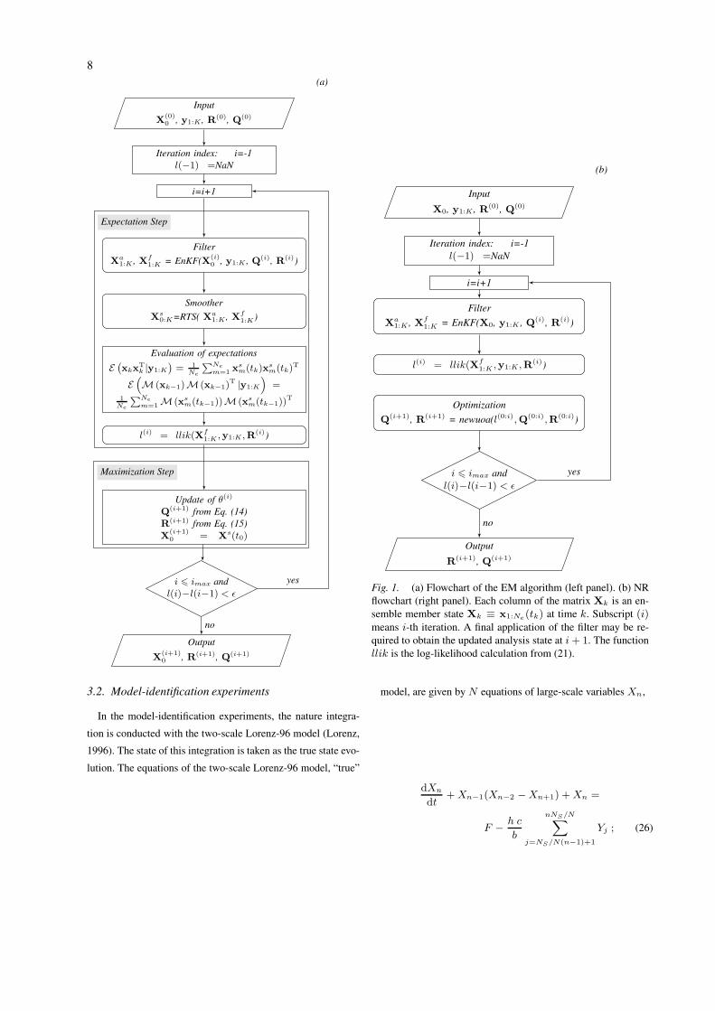
Fig. 1. (a) Flowchart of the EM algorithm (left panel). (b) NR

flowchart (right panel). Each column of the matrix Xk is an en-

semble member state Xk ≡ x1:Ne(tk) at time k. Subscript (i)

means i-th iteration. A final application of the filter may be re-

quired to obtain the updated analysis state at i+ 1. The function

llik is the log-likelihood calculation from (21).

3.2. Model-identification experiments

In the model-identification experiments, the nature integra-

tion is conducted with the two-scale Lorenz-96 model (Lorenz,

1996). The state of this integration is taken as the true state evo-

lution. The equations of the two-scale Lorenz-96 model, “true”

model, are given by N equations of large-scale variables Xn,

dXn

dt+Xn−1(Xn−2 −Xn+1) +Xn =

F −h c

b

nNS/N∑

j=NS/N(n−1)+1

Yj ; (26)

STOCHASTIC PARAMETERIZATION IDENTIFICATION USING MAXIMUM LIKELIHOOD METHODS

9

with n = 1, . . . , N ; and NS equations of small-scale variables

Ym, given by

dYm

dt+ c b Ym+1(Ym+2 − Ym−1) + c Ym =

h c

bXint[(m−1)/NS/N]+1 , (27)

where m = 1, . . . , NS . The two set of equations, (26) and (27),

are assumed to be defined on a periodic domain, X−1 ≡ XN−1,

X0 ≡ XN , XN+1 ≡ X1, and Y0 ≡ YNS, YNS+1 ≡ Y1,

YNS+2 ≡ Y2.

The imperfect model used in the model-identification experi-

ments is the one-scale Lorenz-96 model (23) with a parameter-

ization (24) meant to represent small-scale effects (right-hand

side of (26)).

3.3. Numerical experiment details

As used in previous works (see e.g., Wilks 2005; Pulido et al.

2016), we set N = 8 and M = 256 for the large- and small-

scale variables respectively. The constants are set to the standard

values b = 10, c = 10 and h = 1. The ordinary differential

equations (26)-(27) are solved by a fourth-order Runge-Kutta

algorithm. The time step is set to dt = 0.001 for integrating

(26) and (27).

For the model-identification experiments, we aim to mimic

the dynamics of the large-scale equations of the two-scale

Lorenz-96 system with the one-scale Lorenz-96 system (23)

forced by a physical parameterization (24). In other words,

our nature is the two-scale model, while our imperfect coarse-

grained model is the forced one-scale model. For this reason,

we take 8 variables for the one-scale Lorenz-96 model for the

perfect-model experiments (as the number of large-scale vari-

ables in the model-identification experiments). Equations (23)

are also solved by a fourth-order Runge-Kutta algorithm. The

time step is also set to dt = 0.001.

The EnKF implementation we use is the ensemble transform

Kalman filter (Hunt et al., 2007) without localization. A short

description of the ensemble transform Kalman filter is given in

the Appendix. The time interval between observations (cycle) is

0.05 (an elapsed time of 0.2 represents about 1 day in the real

atmosphere considering the error growth rates; Lorenz, 1996).

The number of ensemble members is set to Ne = 50. The num-

ber of assimilation cycles (observation times) is K = 500. This

is the “evidencing window” (Carrassi et al., 2017) in which we

seek for the optimal statistical parameters. The measurement

variance error is set to αR = 0.5 except otherwise stated. We

do not use any inflation factor, since the model error covariance

matrix is estimated.

The optimization method used in the NR maximization is

“newuoa” (Powell, 2006). This is an unconstrained minimiza-

tion algorithm which does not require derivatives. It is suitable

for control spaces of about a few hundred dimensions. This

derivative-free method could eventually permit to extend the

NR maximization method to cases in which the state evolution

(1) incorporates a non-additive model error.

4. Results

4.1. Perfect-model experiment: Estimation of model

noise parameters

The nature integration is obtained from the one-scale Lorenz-

96 model (23) with a constant forcing of a0 = 17 without

higher orders in the parameterization; in other words a one-scale

Lorenz-96 model with an external forcing of F = 17. Informa-

tion quantifiers show that for an external forcing of F = 17, the

Lorenz-96 model is in a chaotic regime with maximal statisti-

cal complexity (Pulido and Rosso, 2017). The true model noise

covariance is defined by Qt = αtQI with αt

Q = 1.0 (true pa-

rameter values are denoted by a t superscript). The observations

are taken from the nature integration and perturbed using (22).

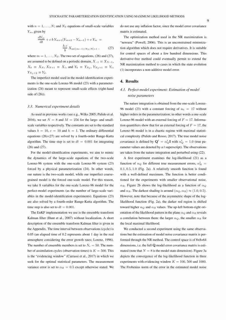
A first experiment examines the log-likelihood (21) as a

function of αQ for different true measurement errors, αtR =

0.1, 0.5, 1.0 (Fig. 2a). A relatively smooth function is found

with a well-defined maximum. The function is better condi-

tioned for the experiments with smaller observational noise,

αR. Figure 2b shows the log-likelihood as a function of αQ

and αR. The darkest shading is around (αQ, αR) ≈ (1.0, 0.5).

However, note that because of the asymmetric shape of the log-

likelihood function (Fig. 2a), the darker red region is shifted

toward higher αQ and αR values. The up-left bottom-right ori-

entation of the likelihood pattern in the plane αQ and αR reveals

a correlation between them: the larger αQ, the smaller αR for

the local maximal likelihood.

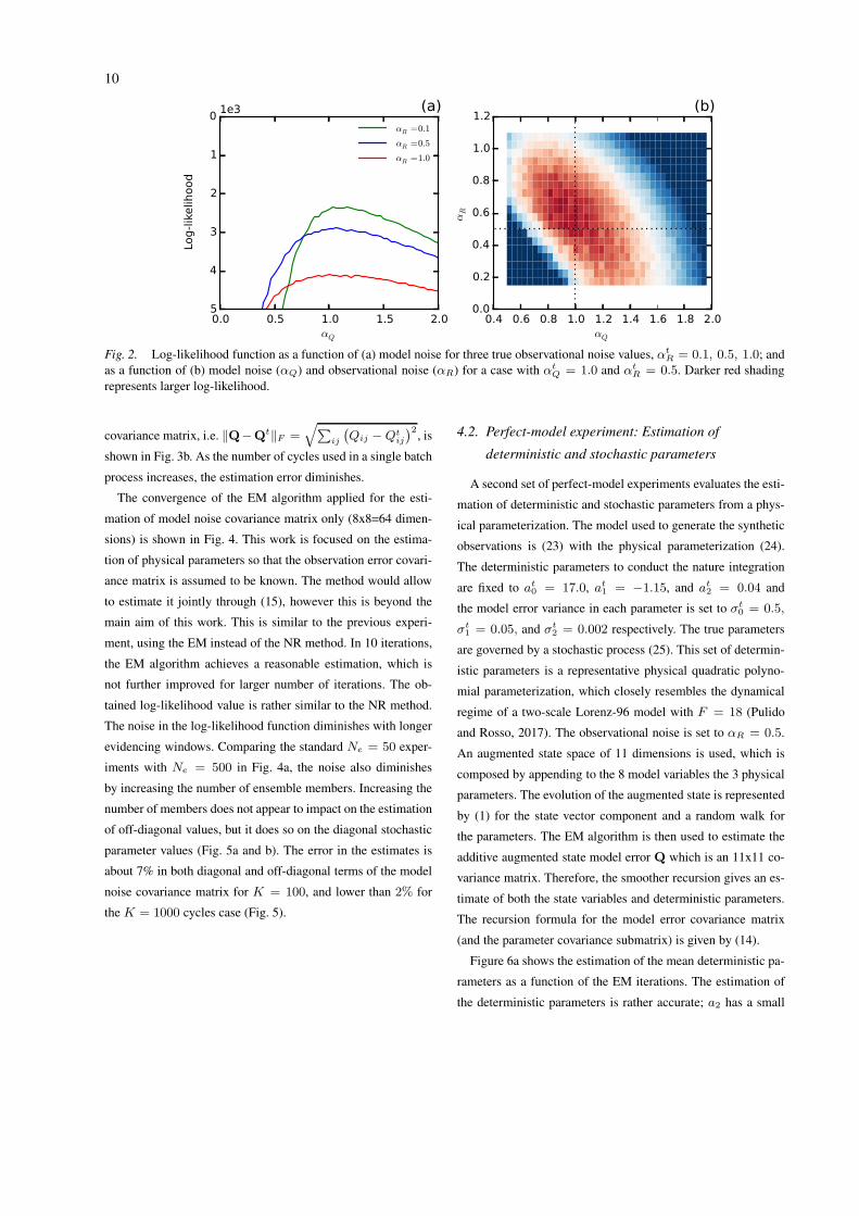
We conducted a second experiment using the same observa-

tions but the estimation of model noise covariance matrix is per-

formed through the NR method. The control space is of 8x8=64

dimensions, i.e. the full Q model error covariance matrix is esti-

mated (note that N = 8 is the model state dimension). Figure 3a

depicts the convergence of the log-likelihood function in three

experiments with evidencing window K = 100, 500 and 1000.

The Frobenius norm of the error in the estimated model noise

10

0.0 0.5 1.0 1.5 2.0αQ

−5

−4

−3

−2

−1

0

Log-likelih

ood

1e3 (a)αR =0.1

αR =0.5

αR =1.0

0.4 0.6 0.8 1.0 1.2 1.4 1.6 1.8 2.0αQ

0.0

0.2

0.4

0.6

0.8

1.0

1.2

αR

(b)

Fig. 2. Log-likelihood function as a function of (a) model noise for three true observational noise values, αtR = 0.1, 0.5, 1.0; and

as a function of (b) model noise (αQ) and observational noise (αR) for a case with αtQ = 1.0 and αt

R = 0.5. Darker red shading

represents larger log-likelihood.

covariance matrix, i.e. ‖Q−Qt‖F =√

∑

ij

(

Qij −Qtij

)2, is

shown in Fig. 3b. As the number of cycles used in a single batch

process increases, the estimation error diminishes.

The convergence of the EM algorithm applied for the esti-

mation of model noise covariance matrix only (8x8=64 dimen-

sions) is shown in Fig. 4. This work is focused on the estima-

tion of physical parameters so that the observation error covari-

ance matrix is assumed to be known. The method would allow

to estimate it jointly through (15), however this is beyond the

main aim of this work. This is similar to the previous experi-

ment, using the EM instead of the NR method. In 10 iterations,

the EM algorithm achieves a reasonable estimation, which is

not further improved for larger number of iterations. The ob-

tained log-likelihood value is rather similar to the NR method.

The noise in the log-likelihood function diminishes with longer

evidencing windows. Comparing the standard Ne = 50 exper-

iments with Ne = 500 in Fig. 4a, the noise also diminishes

by increasing the number of ensemble members. Increasing the

number of members does not appear to impact on the estimation

of off-diagonal values, but it does so on the diagonal stochastic

parameter values (Fig. 5a and b). The error in the estimates is

about 7% in both diagonal and off-diagonal terms of the model

noise covariance matrix for K = 100, and lower than 2% for

the K = 1000 cycles case (Fig. 5).

4.2. Perfect-model experiment: Estimation of

deterministic and stochastic parameters

A second set of perfect-model experiments evaluates the esti-

mation of deterministic and stochastic parameters from a phys-

ical parameterization. The model used to generate the synthetic

observations is (23) with the physical parameterization (24).

The deterministic parameters to conduct the nature integration

are fixed to at0 = 17.0, at

1 = −1.15, and at2 = 0.04 and

the model error variance in each parameter is set to σt0 = 0.5,

σt1 = 0.05, and σt

2 = 0.002 respectively. The true parameters

are governed by a stochastic process (25). This set of determin-

istic parameters is a representative physical quadratic polyno-

mial parameterization, which closely resembles the dynamical

regime of a two-scale Lorenz-96 model with F = 18 (Pulido

and Rosso, 2017). The observational noise is set to αR = 0.5.

An augmented state space of 11 dimensions is used, which is

composed by appending to the 8 model variables the 3 physical

parameters. The evolution of the augmented state is represented

by (1) for the state vector component and a random walk for

the parameters. The EM algorithm is then used to estimate the

additive augmented state model error Q which is an 11x11 co-

variance matrix. Therefore, the smoother recursion gives an es-

timate of both the state variables and deterministic parameters.

The recursion formula for the model error covariance matrix

(and the parameter covariance submatrix) is given by (14).

Figure 6a shows the estimation of the mean deterministic pa-

rameters as a function of the EM iterations. The estimation of

the deterministic parameters is rather accurate; a2 has a small

STOCHASTIC PARAMETERIZATION IDENTIFICATION USING MAXIMUM LIKELIHOOD METHODS

11

0 5 10 15 20 25 30 35 40

NR i era ion

−9.5

−9.0

−8.5

−8.0

−7.5

−7.0

−6.5

−6.0

−5.5

Log-lik

elih

ood

(a)

0 5 10 15 20 25 30 35 40

NR iteration

0.0

0.1

0.2

0.3

0.4

0.5

0.6

||Q−Q

t|| F

(b)K=100K=500K=1000

Fig. 3. Convergence of the NR maximization as a function of the iteration of the outer loop for different evidencing window

lengths. (a) Log-likelihood function. (b) Frobenius norm of the model noise estimation error.

0 20 40 60 80 100

EM i era ion

−6.8

−6.6

−6.4

−6.2

−6.0

−5.8

−5.6

Log-lik

elih

ood

(a)

0 20 40 60 80 100

EM iteration

10-4

10-3

10-2

10-1

||Q−Q

t|| F

(b)K=100K=500K=1000K=500, Ne=500

Fig. 4. Convergence of the EM algorithm as a function of the iteration for different observation time lengths (evidencing window).

An experiment with Ne = 500 ensemble members and K = 500 is also shown. (a) Log-likelihood function. (b) The Frobenius

norm of the model noise estimation error.

0 20 40 60 80 100

EM Iteration

0.9

1.0

1.1

1.2

1.3

1.4

1.5

1.6

1.7

1.8

Est

ima

ted

Q.

Dia

go

na

l v

alu

es

(a)K=100K=500K=1000K=500, Ne=500

0 20 40 60 80 100

EM Iteration

0.00

0.01

0.02

0.03

0.04

0.05

0.06

0.07

0.08

Est

ima

ted

Q.

Off

-dia

go

na

l v

alu

es

(b)

Fig. 5. Estimated model noise as a function of the iteration in the EM algorithm. (a) Mean diagonal model noise (true value is 1.0).

(b) Mean off-diagonal absolute model noise value (true value is 0.0).

12

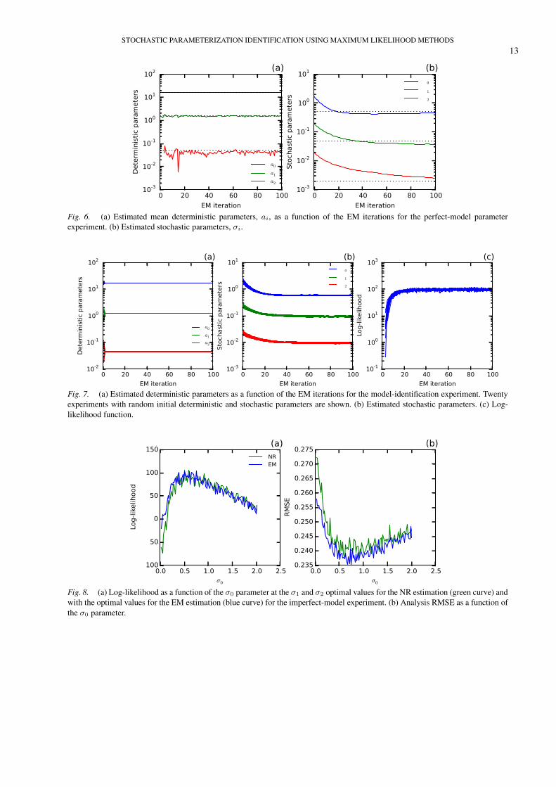
true value and it presents the lowest sensitivity. The estimation

of the stochastic parameters by the EM algorithm converges

rather precisely to the true stochastic parameters (Fig. 6b).

The convergence requires of about 80 iterations. The estimated

model error for the state variables is in the order of 5 × 10−2.

This represents the additive inflation needed by the filter for an

optimal convergence. It establishes a lower threshold for the es-

timation of additive stochastic parameters.

A similar experiment was conducted with NR maximiza-

tion for the same synthetic observations. A scaling of Sσ =

(1, 10, 100) was included in the optimization to increase the

condition number. A good convergence was obtained with the

optimization algorithm. The estimated optimal parameter val-

ues are σ0 = 0.38 σ1 = 0.060 σ2 = 0.0025 for which the

log-likelihood is l = −491. The estimation is reasonable with

a relative error of about 25%.

4.3. Model-identification experiment: Estimation of the

deterministic and stochastic parameters

As a proof-of-concept model-identification experiment, we

now use synthetic observations with an additive observational

noise of αR = 0.5 taken from the nature integration of the two-

scale Lorenz-96 model with F = 18. On the other hand, the

one-scale Lorenz-96 model is used in the ensemble Kalman fil-

ter with a physical parameterization that includes the quadratic

polynomial function, (24), and the stochastic process (25). The

deterministic parameters are estimated through an augmented

state space while the stochastic parameters are optimized via the

algorithm for the maximization of the log-likelihood function.

The model error covariance estimation is constrained for these

experiments to the three stochastic parameters alone. Figure 7a

shows the estimated deterministic parameters as a function of

the EM iterations. Twenty experiments with different initial de-

terministic parameters and initial stochastic parameter values

were conducted. The deterministic parameter estimation does

not manifest a significant sensitivity to the stochastic parame-

ter values. The mean estimated values are a0 = 17.3, a1 =

−1.25 and a3 = 0.0046. Note that the deterministic parame-

ter values estimated with information quantifiers in Pulido and

Rosso (2017) for the two-scale Lorenz-96 with F = 18 are

(a0, a1, a2) = (17.27,−1.15, 0.037). Figure 7b depicts the

convergence of the stochastic parameters. The mean of the op-

timal stochastic parameter values are σ0 = 0.60, σ1 = 0.094

and σ2 = 0.0096 with the log-likelihood value being 98.8 (sin-

gle realization). The convergence of the log-likelihood is shown

in Fig. 7c.

NR maximization is applied to the same set of synthetic

observations. The mean estimated deterministic and stochas-

tic parameters are (a0, a1, a2) = (17.2,−1.24, 0.0047) and

(σ0, σ1, σ2) = (0.59, 0.053, 0.0064) from 20 optimizations.

As in the EM experiment, only the three stochastic parame-

ters were estimated as statistical parameters. Preliminary ex-

periments with the full augmented model error covariance gave

smaller estimated σ0 values and nonnegligible model error vari-

ance (not shown). The log-likelihood function (Fig. 8a) and the

analysis root-mean-square error (RMSE, Fig. 8b) are shown as

a function of σ0 at the σ1 and σ2 optimal values given by the

Newton-Rapshon method (green curve) and at the σ1 and σ2 op-

timal values given by the EM algorithm (blue curve). The log-

likelihood values are indistinguishable. A slightly smaller anal-

ysis RMSE is obtained for the EM algorithm (Fig. 8b), which

is likely related to the improvement with the iterations of the

initial prior distribution in the EM algorithm, while this distri-

bution is fixed in the NR method.

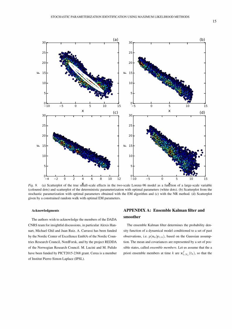
Long integrations (106 time cycles) of the nature model and

the identified coarse-grained models were conducted to evaluate

the parameterizations. The true effects of the small-scale vari-

ables on a large-scale variable from the two-scale Lorenz-96

model are shown in Fig. 9 as a function of the large-scale vari-

able. This true scatterplot is obtained by evaluating the right-

hand side of (26). The deterministic quadratic parameterization

with the optimal parameters from the EnKF is also represented

in Fig. 9(a). A poor representation of the functional form and

variability is obtained. Figure 9(b) shows the scatterplot with

a stochastic parameterization which stochastic parameters are

the ones estimated with EM algorithm, while Fig. 9(c) shows

it for the stochastic parameters estimated with the NR method.

The two methods, NR and EM, give scatterplots of the param-

eterization which are almost indistinguishable and improve the

small-scale representation with respect to the deterministic pa-

rameterization. Figure 9(d) shows the scatterplot resulting from

the quadratic parameterization using a random walk for the pa-

rameters set to the estimated values with the EM algorithm. The

values of the parameters are limited to the ai ± 4σi range. The

parameter values need to be constrained, because for these long

free simulations, some parameter values given by the random

walk produce numerical instabilities in the Lorenz-96 model

(Pulido et al., 2016). The stochastic parameterization which was

identified by the statistical learning technique improves substan-

STOCHASTIC PARAMETERIZATION IDENTIFICATION USING MAXIMUM LIKELIHOOD METHODS

13

0 20 40 60 80 100

EM iteration

10-3

10-2

10-1

100

101

102

Determ

inistic parameters

(a)

a0

a1a2

0 20 40 60 80 100

EM iteration

10-3

10-2

10-1

100

101

Stoch

astic parameters

(b)σ0

σ1σ2

Fig. 6. (a) Estimated mean deterministic parameters, ai, as a function of the EM iterations for the perfect-model parameter

experiment. (b) Estimated stochastic parameters, σi.

0 20 40 60 80 100

EM iteration

10-2

10-1

100

101

102

Dete

rmin

istic

para

mete

rs

(a)

a0

a1a2

0 20 40 60 80 100

EM iteration

10-3

10-2

10-1

100

101

Sto

chast

ic p

ara

mete

rs

(b)σ0

σ1σ2

0 20 40 60 80 100

EM iteration

10-1

100

101

102

103

Log-lik

elih

ood

(c)

Fig. 7. (a) Estimated deterministic parameters as a function of the EM iterations for the model-identification experiment. Twenty

experiments with random initial deterministic and stochastic parameters are shown. (b) Estimated stochastic parameters. (c) Log-

likelihood function.

0.0 0.5 1.0 1.5 2.0 2.5σ0

−100

−50

0

50

100

150

Log-likelih

ood

(a)NREM

0.0 0.5 1.0 1.5 2.0 2.5σ0

0.235

0.240

0.245

0.250

0.255

0.260

0.265

0.270

0.275

RMSE

(b)

Fig. 8. (a) Log-likelihood as a function of the σ0 parameter at the σ1 and σ2 optimal values for the NR estimation (green curve) and

with the optimal values for the EM estimation (blue curve) for the imperfect-model experiment. (b) Analysis RMSE as a function of

the σ0 parameter.

14

tially the functional form of the effects of the small-scale vari-

ables. Using a constrained random walk appears to give the best

simulation.

5. Conclusions

Two methods, the EnKF-EM and EnKF-NR, have been intro-

duced to characterize physical parameterizations in stochastic

nonlinear multi-scale dynamical systems from noisy observa-

tions, which include the estimation of deterministic and stochas-

tic parameters. Both methods determine the maximum of the

observation likelihood –maximum of the model evidence– in a

time interval in which a set of spatio-temporally distributed ob-

servations are available. They use the ensemble Kalman filter to

combine observations with model predictions. The methods are

first evaluated in a controlled model experiment in which the

true parameters are known and then, in the two-scale Lorenz-96

dynamics which is represented with a stochastic coarse-grained

model. The methods do not require neither inflation factors nor

any other tunable parameters. The performance of the meth-

ods is excellent, even in the presence of moderate observational

noise.

The estimation based on the expectation-maximization algo-

rithm gives very promising results in these medium-sized ex-

periments (≈100 parameters). About 50 iterations are needed

to achieve an estimation error lower than 10% using 100 ob-

servation times. Using a longer observation time inverval, the

accuracy is improved. The estimation of stochastic parameters

included the case of additive, i.e. a0, and multiplicative param-

eters, i.e. a1Xn and a2X2n. The number of ensemble members

has a strong impact on the stochastic parameter variance, while

the length of the observation time interval appears to have a

stronger impact on the stochastic parameter correlations.

The estimation based on the NR method also presents good

convergence for the perfect-model experiment with an additive

stochastic parameter. For the more realistic model-identification

experiments, the model evidence presents some noise which

may affect the convergence. For higher dimensional problems,

optimization algorithms that use the gradient of the likelihood

to the statistical parameters need to be implemented. Moreover,

the use of simulated annealing or other stochastic gradient opti-

mization techniques suitable for noisy cost functions would be

required.

Both estimation methods can be applied to a set of different

dynamical models to address which one is more reliable given a

set of noisy observations; the so called “model selection” prob-

lem. A comparison of the likelihood from the different models

with the optimal parameters gives a measure of the model fi-

delity to the observations. Majda and Gershgorin (2011) seeked

to improve imperfect models by adding stochastic forcing and

used a measure from information theory that gives the clos-

est model distribution to the observed probability distribution.

The model-identification experiments in the current work can

be viewed as pursuing a similar objective, stochastic processes

are added to the physical parameterization to improve the model

representation of the unresolved processes. A sequential Monte

Carlo filter is used between observations so that their error is

accounted in the estimation. In both cases, the methodologies

are based on Gaussian assumptions.

Hannart et al. (2016) proposed to apply the observation like-

lihood function, model evidence, that results from assimilating

a set of observations, for the detection and attribution of climate

change. They suggest to evaluate the likelihood in two possi-

ble model configurations, one with the current anthropogenic

forcing scenario (factual world) and one with the preindustrial

forcing scenario (contrafactual world). If the evidencing win-

dow where the observations are located includes, for instance,

an extreme event then one could determine the fraction of at-

tributable risk as the fraction of the change in the observation

likelihood of the extreme event which is attributable to the an-

thropogenic forcing.

The increase of data availability in many areas has fostered

the number of applications of the ensemble Kalman filter. In

particular, it has been used for influenza forecasting (Shaman

et al., 2013) and for determining a neural network structure

(Hamilton et al., 2013). The increase in spatial and temporal

resolution of data offers great opportunities for understanding

multi-scale strongly-coupled systems such as atmospheric and

oceanic dynamics. This has lead to the proposal of purely data-

driven modeling which uses past observations to reconstruct the

dynamics through the ensemble Kalman filter without a dy-

namical model (Hamilton et al., 2016; Lguensat et al., 2017).

The use of automatic statistical learning techniques that can use

measurements for improvement of multi-scale models is also a

promising venue. Following this recent stream of research, in

this work we propose the coupling of the EM algorithm and NR

method with the ensemble Kalman filter which may be applica-

ble to a wide range of multi-scale systems to improve the repre-

sentation of the complex interactions between different scales.

STOCHASTIC PARAMETERIZATION IDENTIFICATION USING MAXIMUM LIKELIHOOD METHODS

15

−10 −5 0 5 10 15

x

0

5

10

15

20

25

30F

(a)

−5 0 5 10 15

x

0

5

10

15

20

25

30

F

(b)

−4 −2 0 2 4 6 8 10 12

x

0

5

10

15

20

25

30

F

(c)

−10 −5 0 5 10 15

x

0

5

10

15

20

25

30

F

(d)

Fig. 9. (a) Scatterplot of the true small-scale effects in the two-scale Lorenz-96 model as a function of a large-scale variable

(coloured dots) and scatterplot of the deterministic parameterization with optimal parameters (white dots). (b) Scatterplot from the

stochastic paramerization with optimal parameters obtained with the EM algorithm and (c) with the NR method. (d) Scatterplot

given by a constrained random walk with optimal EM parameters.

Acknowledgments

The authors wish to acknowledge the members of the DADA

CNRS team for insightful discussions, in particular Alexis Han-

nart, Michael Ghil and Juan Ruiz. A. Carrassi has been funded

by the Nordic Center of Excellence EmblA of the Nordic Coun-

tries Research Council, NordForsk, and by the project REDDA

of the Norwegian Research Council. M. Lucini and M. Pulido

have been funded by PICT2015-2368 grant. Cerea is a member

of Institut Pierre-Simon Laplace (IPSL).

APPENDIX A: Ensemble Kalman filter and

smoother

The ensemble Kalman filter determines the probability den-

sity function of a dynamical model conditioned to a set of past

observations, i.e. p(xk|y1:k), based on the Gaussian assump-

tion. The mean and covariances are represented by a set of pos-

sible states, called ensemble members. Let us assume that the a

priori ensemble members at time k are xf1:Ne

(tk), so that the

16

empirical mean and covariance of the a priori hidden state are

xf (tk) =

1

Ne

Ne∑

m=1

xfm(tk),

Pf (tk) =

1

Ne − 1X

f (tk)[Xf (tk)]

T, (A1)

where Xf (tk) is a matrix with the ensemble member perturba-

tions, xfm(tk)− xf (tk), as the m-ith column.

To obtain the estimated hidden state, called analysis state, the

observations are combined statistically with the a priori model

state using the Kalman filter equations. In the case of the ensem-

ble transformed Kalman filter (Hunt et al., 2007), the analysis

state is a linear combination of the Ne ensemble member per-

turbations,

xa = x

f +Xfw

a, P

a = XfP

a(Xf )T. (A2)

The optimal ensemble member weights wa are obtained con-

sidering the distance between the projection of member states

to the observational space, yfm ≡ H(xf

m), and observations y.

These weights and the analysis covariance matrix in the pertur-

bation space are

wa = P

a(Yf )TR−1[y − yf ],

Pa = [(Ne − 1)I+ (Yf )TR−1

Yf ]−1

. (A3)

All the quantities in (A2) and (A3) are at time tk so that the

time dependence is omitted for clarity. A detailed derivation of

(A2) and (A3) and a thorough description of the ensemble trans-

formed Kalman filter and its numerical implementation can be

found in Hunt et al. (2007).

To determine each ensemble member of the analysis state,

the ensemble transformed Kalman filter uses the square root of

the analysis covariance matrix, thus it belongs to the so-called

square-root filters,

xam = x

f +Xfw

am (A4)

where the perturbations of wam are the columns of Wa =

[(Ne − 1)Pa]1/2.

The analysis state is evolved to the time of the next available

observation tk+1 through the dynamical model equations which

give the a priori or forecasted state,

xfm(tk+1) = M(xa

m(tk)). (A5)

The smoother determines the probability density function of

a dynamical model conditioned to a set of past and future ob-

servations, i.e. p(xk|y1:K), based on the Gaussian assumption.

Applying the Rauch-Tung-Striebel smoother retrospective for-

mula to each ensemble member (Cosme et al., 2012),

xsm(tk) = x

am(tk) +K

s(tk)[xsm(tk+1)− x

fm(tk+1)], (A6)

where Ks(tk) = Pa(tk)MTk→k+1[P

f (tk+1)]−1, and

Mk→k+1 being the linear tangent model. For the application

of the smoother in conjunction with the ensemble transformed

Kalman filter, the smoother gain is reexpressed as

Ks(tk) = X

f (tk)Wa[Xf (tk+1)]

†. (A7)

In practice, the peusdo-inversion of the forecast state perturba-

tion matrix Xf required in (A7) is conducted through singular

value decomposition.

References

Anderson, J. (2001). An ensemble adjustment Kalman filter for data

assimilation. Mon. Wea. Rev., 142:2884–2903.

Bishop, C. (2006). Pattern recognition and machine learning. Springer.

Cappe, O., Moulines, E., and Ryden, T. (2005). Inference in Hidden

Markov Models. Springer. New York.

Carrassi, A., Bocquet, M., Hannart, A., and Ghil, M. (2017). Estimat-

ing model evidence using data assimilation. Q. J. R. Meteorol. Soc.,

143:866–880.

Carrassi, A. and Vannitsem, S. (2011). State and parameter estima-

tion with the extended Kalman filter: an alternative formulation of

the model error dynamics. Q. J. R. Meteorol. Soc., 137:435–451.

Christensen, H., Moroz, I. M., and Palmer, T. N. (2015). Stochastic and

perturbed parameter representations of model uncertainty in convec-

tion parameterization. J. Atmos. Sci., 72:2525–2544.

Cosme, E., Verron, J., Brasseur, P., Blum, J., and Auroux, D. (2012).

Smoothing problems in a Bayesian framework and their linear gaus-

sian solutions. Monthly Weather Review, 140:683–695.

Delsole, T. and Yang, X. (2010). State and parameter estimation in

stochastic dynamical models. Physica D, 239:1781–1788.

Dempster, A., Laird, N., and Rubin, D. (1977). Maximum likelihood

from incomplete data via the EM algorithm. J. of the Royal Stat. Soc.

Series B, pages 1–38.

Dreano, D., Tandeo, P., Pulido, M., Ait-El-Fquih, B., Chonavel, T., and

Hoteit, I. (2017). Estimation of error covariances in nonlinear state-

space models using the expectation maximization algorithm. Q. J.

Roy. Meteorol. Soc., 142:1877–1885.

Evensen, G. (1994). Sequential data assimilation with a nonlinear quasi-

geostrophic model using monte carlo methods to forecast error statis-

tics. J. Geophys. Res., 99:10143–10162.

Evensen, G. (2003). The ensemble Kalman filter: Theoretical formula-

tion and practical implementation. Ocean dynamics, 53:343–367.

Ghahramani, Z. and Roweis, S. (1999). Learning nonlinear dynamical

STOCHASTIC PARAMETERIZATION IDENTIFICATION USING MAXIMUM LIKELIHOOD METHODS

17

systems using an EM algorithm, volume 11, pages 431–437. MIT

press.

Hamilton, F., Berry, T., Peixoto, N., and Sauer, T., . (2013). Real-time

tracking of neuronal network structure using data assimilation. Phys.

Rev. E, 88:052715.

Hamilton, F., Berry, T., and Sauer, T. (2016). Ensemble Kalman filtering

without a model. Physical Review X, 6:011021.

Hannart, A., Carrassi, A., Bocquet, M., Ghil, M., Naveau, P., Pulido,

M., Ruiz, J., and Tandeo, P. (2016). Dada: Data Assimilation for

the Detection and Attribution of weather and climate-related events.

Climatic Change, 136:155–174.

Hunt, B., Kostelich, E. J., and Szunyogh, I. (2007). Efficient data

assimilation for spatio-temporal chaos: A local ensemble transform

Kalman filter. Physica D, 77:437–471.

Jazwinski, A. H. (1970). Stochastic and Filtering Theory. Mathematics

in Sciences and Engineering Series. 64. Academic Press, 376 pp.

Kalnay, E. (2002). Atmospheric Modeling, Data Assimilation, and Pre-

dictability. Cambridge University Press, Cambridge, UK.

Katsoulakis, M., Majda, A., and Vlachos, D. (2003). Coarse-grained

stochastic processes for microscopic lattice systems. Proc Natl Acad

Sci, 100:782–787.

Kondrashov, D., Ghil, M., and Shprits, Y. (2011). Lognormal Kalman

filter for assimilating phase space density data in the radiation belts.

Space Weather, 9:11.

Lguensat, R., Tandeo, P., Fablet, R., Pulido, M., and Ailliot, P. (2017).

The analog ensemble-based data assimilation. Mon. Wea. Rev.

Lorenz, E. (1996). Predictability—A problem partly solved, pages 1–18.

ECMWF, Reading, UK.

Lott, F., Guez, L., and Maury, P. (2012). A stochastic parameteriza-

tion of nonorographic gravity waves: Formalism and impact on the

equatorial stratosphere. Geophys. Res. Lett., 39:6.

Majda, A. and Gershgorin, B. (2011). Improving model fidelity and

sensitivity for complex systems through empirical information the-

ory. Proc Natl Acad Sci, 100:10044–10049.

Mason, P. and Thomson, D. (1992). Stochastic backscatter in large-eddy

simulations of boundary layers. J. Fluid Mech., 242:51–78.

Neal, R. and Hinton, G. (1999). A view of the EM algorithm that justifies

incremental, sparse and other variants. Springer.

Nicolis, N. (2004). Dynamics of model error: The role of unresolved

scales revisited. J. Atmos. Sci., 61:1740–1753.

Palmer, T. (2001). A nonlinear dynamical perspective on model er-

ror: A proposal for non-local stochastic-dynamic parameterization

in weather and climate prediction models. Q.J.R. Meteorol. Soc.,

127:279–304.

Powell, M. (2006). The NEWUOA software for unconstrained optimiza-

tion without derivatives, pages 255–297. Springer.

Pulido, M. and Rosso, O. (2017). Model selection: Using information

measures from ordinal symbolic analysis to select model sub-grid

scale parameterizations. In press in J. Atmos. Sci.

Pulido, M., Scheffler, G., Ruiz, J., Lucini, M., and Tandeo, P. (2016).

Estimation of the functional form of subgrid-scale schemes using

ensemble-based data assimilation: a simple model experiment. Q.

J. Roy. Meteorol. Soc., 142:2974–2984.

Raanes, P. (2016). On the ensemble Rauch-Tung-Striebel smoother and

its equivalence to the ensemble Kalman smoother. Q. J. R. Meteorol.

Soc., 142:1259–1264.

Ruiz, J., Pulido, M., and Miyoshi, T. (2013a). Estimating parameters

with ensemble-based data assimilation. A review. J. Meteorol. Soc.

Japan, 91:79–99.

Ruiz, J., Pulido, M., and Miyoshi, T. (2013b). Estimating parameters

with ensemble-based data assimilation. Parameter covariance treat-

ment. J. Meteorol. Soc. Japan, 91:453–469.

Santitissadeekorn, N. and Jones, C. (2015). Two-stage filtering for joint

state-parameter estimation. Mon. Wea. Rev., 143:2028–2042.

Shaman, J., Karspeck, A., Yang, W., Tamerius, J., and Lipsitch, M.

(2013). Real-time influenza forecasts during the 20122013 season.

Nature Comm., 4:2837.

Shumway, R. and Stoffer, D. (1982). An approach to time series

smoothing and forecasting using the EM algorithm. J. Time Series

Anal., 3:253–264.

Shutts, G. (2015). A stochastic convective backscatter scheme

for use in ensemble prediction systems. Q.J.R. Meteorol. Soc.,

10.1002/qj.2547.

Stensrud, D. (2009). Parameterization Schemes: Keys to Understanding

Numerical Weather Prediction Models. Cambridge University Press,

Cambridge, UK.

Tandeo, P., Pulido, M., and Lott, F. (2015). Offline estimation of

subgrid-scale orographic parameters using EnKF and maximum

likelihood error covariance estimates. Q. J. Roy. Meteorol. Soc.,

141:383–395.

Wei, G. and Tanner, M. A. (1990). A Monte Carlo implementation of

the EM algorithm and the poor man’s data augmentation algorithms.

J. Amer. Stat. Assoc., 85:699–704.

West, M. and Liu, J. (2001). Combined parameter and state estimation

in simulation-based filtering, pages 197–223. Springer.

Wikle, C. and Berliner (2007). A Bayesian tutorial for data assimilation.

Physica D, 230:1–16.

Wilks, D. S. (2005). Effects of stochastic parametrizations in the Lorenz

96 system. Q. J. R. Meteorol. Soc., 131:389–407.