Stochastic Optimization Techniques for Big Data Machine...
129
Stochastic Optimization Techniques for Big Data Machine Learning Tong Zhang Rutgers University & Baidu Inc. T. Zhang Big Data Optimization 1 / 73
Transcript of Stochastic Optimization Techniques for Big Data Machine...
Stochastic Optimization Techniques for Big DataMachine Learning
Tong Zhang
Rutgers University & Baidu Inc.
T. Zhang Big Data Optimization 1 / 73

Outline
Background:big data optimization in machine learning: special structure
Single machine optimizationstochastic gradient (1st order) versus batch gradient: pros and consalgorithm 1: SVRG (Stochastic variance reduced gradient)algorithm 2: SAGA (Stochastic Average Gradient ameliore)algorithm 3: SDCA (Stochastic Dual Coordinate Ascent)algorithm 4: accelerated SDCA (with Nesterov acceleration)
Distributed optimizationalgorithm 5: accelerated minibatch SDCAalgorithm 6: DANE (Distributed Approximate NEwton-type method)behaves like 2nd order stochastic sampling
T. Zhang Big Data Optimization 2 / 73
Mathematical Problem
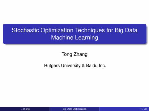
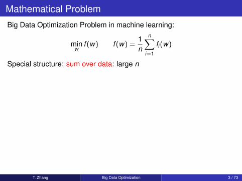
Big Data Optimization Problem in machine learning:
minw
f (w) f (w) =1n
n∑i=1
fi(w)
Special structure: sum over data: large n
Assumptions on loss functionλ-strong convexity:
f (w ′) ≥ f (w) +∇f (w)>(w ′ − w) +λ
2‖w ′ − w‖22︸ ︷︷ ︸
quadratic lower bound
L-smoothness:
fi(w ′) ≤ fi(w) +∇fi(w)>(w ′ − w) +L2‖w ′ − w‖22︸ ︷︷ ︸
quadratic upper bound
T. Zhang Big Data Optimization 3 / 73

Mathematical Problem
Big Data Optimization Problem in machine learning:
minw
f (w) f (w) =1n
n∑i=1
fi(w)
Special structure: sum over data: large n
Assumptions on loss functionλ-strong convexity:
f (w ′) ≥ f (w) +∇f (w)>(w ′ − w) +λ
2‖w ′ − w‖22︸ ︷︷ ︸
quadratic lower bound
L-smoothness:
fi(w ′) ≤ fi(w) +∇fi(w)>(w ′ − w) +L2‖w ′ − w‖22︸ ︷︷ ︸
quadratic upper bound
T. Zhang Big Data Optimization 3 / 73
Example: Computational Advertising
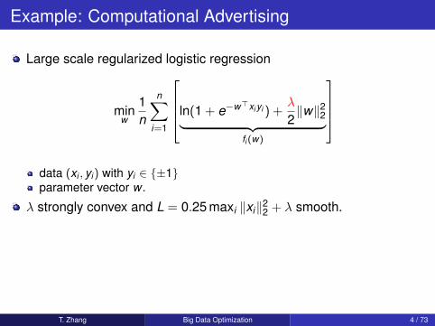
Large scale regularized logistic regression
minw
1n
n∑i=1
ln(1 + e−w>xi yi ) +λ
2‖w‖22︸ ︷︷ ︸
fi (w)
data (xi , yi ) with yi ∈ ±1parameter vector w .
λ strongly convex and L = 0.25 maxi ‖xi‖22 + λ smooth.
big data: n ∼ 10− 100 billionhigh dimension: dim(xi) ∼ 10− 100 billion
How to solve big optimization problems efficiently?
T. Zhang Big Data Optimization 4 / 73

Example: Computational Advertising
Large scale regularized logistic regression
minw
1n
n∑i=1
ln(1 + e−w>xi yi ) +λ
2‖w‖22︸ ︷︷ ︸
fi (w)
data (xi , yi ) with yi ∈ ±1parameter vector w .
λ strongly convex and L = 0.25 maxi ‖xi‖22 + λ smooth.
big data: n ∼ 10− 100 billionhigh dimension: dim(xi) ∼ 10− 100 billion
How to solve big optimization problems efficiently?
T. Zhang Big Data Optimization 4 / 73

Optimization Problem: Communication Complexity
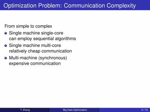
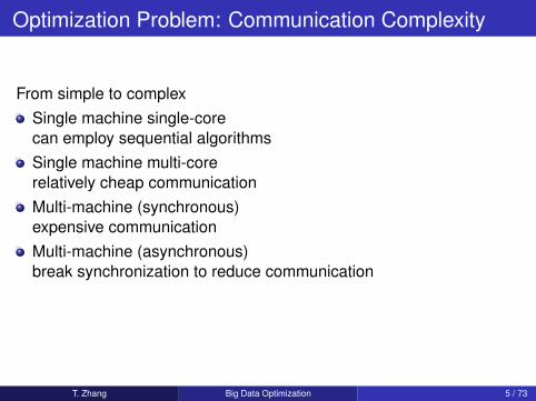
From simple to complexSingle machine single-corecan employ sequential algorithms
Single machine multi-corerelatively cheap communicationMulti-machine (synchronous)expensive communicationMulti-machine (asynchronous)break synchronization to reduce communication
We want to solve simple problem well first, then more complex ones.
T. Zhang Big Data Optimization 5 / 73

Optimization Problem: Communication Complexity
From simple to complexSingle machine single-corecan employ sequential algorithmsSingle machine multi-corerelatively cheap communication
Multi-machine (synchronous)expensive communicationMulti-machine (asynchronous)break synchronization to reduce communication
We want to solve simple problem well first, then more complex ones.
T. Zhang Big Data Optimization 5 / 73
Optimization Problem: Communication Complexity
From simple to complexSingle machine single-corecan employ sequential algorithmsSingle machine multi-corerelatively cheap communicationMulti-machine (synchronous)expensive communication
Multi-machine (asynchronous)break synchronization to reduce communication
We want to solve simple problem well first, then more complex ones.
T. Zhang Big Data Optimization 5 / 73
Optimization Problem: Communication Complexity
From simple to complexSingle machine single-corecan employ sequential algorithmsSingle machine multi-corerelatively cheap communicationMulti-machine (synchronous)expensive communicationMulti-machine (asynchronous)break synchronization to reduce communication
We want to solve simple problem well first, then more complex ones.
T. Zhang Big Data Optimization 5 / 73

Outline
Background:big data optimization in machine learning: special structure
Single machine optimizationstochastic gradient (1st order) versus batch gradient: pros and consalgorithm 1: SVRG (Stochastic variance reduced gradient)algorithm 2: SAGA (Stochastic Average Gradient ameliore)algorithm 3: SDCA (Stochastic Dual Coordinate Ascent)algorithm 4: accelerated SDCA (with Nesterov acceleration)
Distributed optimizationalgorithm 5: accelerated minibatch SDCAalgorithm 6: DANE (Distributed Approximate NEwton-type method)behaves like 2nd order stochastic sampling
T. Zhang Big Data Optimization 6 / 73

Batch Optimization Method: Gradient Descent
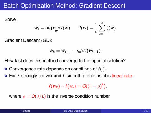
Solve
w∗ = arg minw
f (w) f (w) =1n
n∑i=1
fi(w).
Gradient Descent (GD):
wk = wk−1 − ηk∇f (wk−1).
How fast does this method converge to the optimal solution?
Convergence rate depends on conditions of f (·).For λ-strongly convex and L-smooth problems, it is linear rate:
f (wk )− f (w∗) = O((1− ρ)k ),
where ρ = O(λ/L) is the inverse condition number
T. Zhang Big Data Optimization 7 / 73
Batch Optimization Method: Gradient Descent
Solve
w∗ = arg minw
f (w) f (w) =1n
n∑i=1
fi(w).
Gradient Descent (GD):
wk = wk−1 − ηk∇f (wk−1).
How fast does this method converge to the optimal solution?
Convergence rate depends on conditions of f (·).For λ-strongly convex and L-smooth problems, it is linear rate:
f (wk )− f (w∗) = O((1− ρ)k ),
where ρ = O(λ/L) is the inverse condition number
T. Zhang Big Data Optimization 7 / 73

Stochastic Approximate Gradient Computation
If
f (w) =1n
n∑i=1
fi(w),
GD requires the computation of full gradient, which is extremely costly
∇f (w) =1n
n∑i=1
∇fi(w)
Idea: stochastic optimization employs random sample (mini-batch) B
to approximate
∇f (w) ≈ 1|B|∑i∈B
∇fi(w)
It is an unbiased estimatormore efficient computation but introduces variance
T. Zhang Big Data Optimization 8 / 73

SGD versus GD
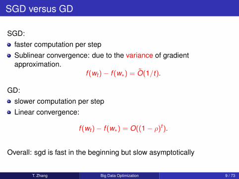
SGD:faster computation per stepSublinear convergence: due to the variance of gradientapproximation.
f (wt )− f (w∗) = O(1/t).
GD:slower computation per stepLinear convergence:
f (wt )− f (w∗) = O((1− ρ)t ).
Overall: sgd is fast in the beginning but slow asymptotically
T. Zhang Big Data Optimization 9 / 73
SGD versus GD
SGD:faster computation per stepSublinear convergence: due to the variance of gradientapproximation.
f (wt )− f (w∗) = O(1/t).
GD:slower computation per stepLinear convergence:
f (wt )− f (w∗) = O((1− ρ)t ).
Overall: sgd is fast in the beginning but slow asymptotically
T. Zhang Big Data Optimization 9 / 73

SGD versus GD
stochastic gradient descent
computational cost
training error
gradient descent
One strategy:use sgd first to trainafter a while switch to batch methods such as LBFGS.
However, one can do better
T. Zhang Big Data Optimization 10 / 73

SGD versus GD
stochastic gradient descent
computational cost
training error
gradient descent
One strategy:use sgd first to trainafter a while switch to batch methods such as LBFGS.
However, one can do betterT. Zhang Big Data Optimization 10 / 73

Improving SGD via Variance Reduction
GD converges fast but computation is slowSGD computation is fast but converges slowly
slow convergence due to inherent variance
SGD as a statistical estimator of gradient:let gi = ∇fi .unbaisedness: E gi = 1
n
∑ni=1 gi = ∇f .
error of using gi to approx ∇f : variance E‖gi − Egi‖22.
Statistical thinking:relating variance to optimizationdesign other unbiased gradient estimators with smaller variance
T. Zhang Big Data Optimization 11 / 73
Improving SGD using Variance Reduction
The idea leads to modern stochastic algorithms for big data machinelearning with fast convergence rate
Collins et al (2008): For special problems, with a relativelycomplicated algorithm (Exponentiated Gradient on dual)Le Roux, Schmidt, Bach (NIPS 2012): A variant of SGD called SAG(stochastic average gradient) and later SAGA (Defazio, Bach,Lacoste-Julien, NIPS 2014)Johnson and Z (NIPS 2013): SVRG (Stochastic variance reducedgradient)Shalev-Schwartz and Z (JMLR 2013): SDCA (Stochastic DualCoordinate Ascent) , and later a variant with Zheng Qu and PeterRichtarik
T. Zhang Big Data Optimization 12 / 73

Outline
Background:big data optimization in machine learning: special structure
Single machine optimizationstochastic gradient (1st order) versus batch gradient: pros and consalgorithm 1: SVRG (Stochastic variance reduced gradient)algorithm 2: SAGA (Stochastic Average Gradient ameliore)algorithm 3: SDCA (Stochastic Dual Coordinate Ascent)algorithm 4: accelerated SDCA (with Nesterov acceleration)
Distributed optimizationalgorithm 5: accelerated minibatch SDCAalgorithm 6: DANE (Distributed Approximate NEwton-type method)behaves like 2nd order stochastic sampling
T. Zhang Big Data Optimization 13 / 73
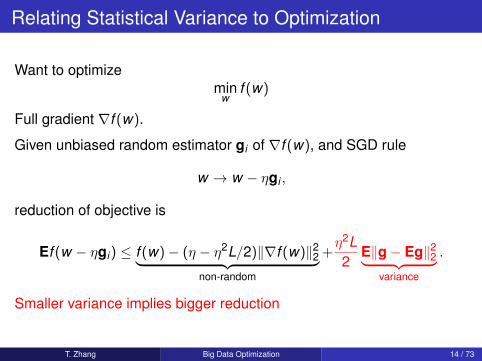
Relating Statistical Variance to Optimization
Want to optimizemin
wf (w)
Full gradient ∇f (w).
Given unbiased random estimator gi of ∇f (w), and SGD rule
w → w − ηgi ,
reduction of objective is
Ef (w − ηgi) ≤ f (w)− (η − η2L/2)‖∇f (w)‖22︸ ︷︷ ︸non-random
+η2L2
E‖g− Eg‖22︸ ︷︷ ︸variance
.
Smaller variance implies bigger reduction
T. Zhang Big Data Optimization 14 / 73

Statistical Thinking: variance reduction techniques
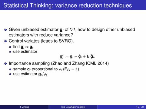
Given unbiased estimator gi of ∇f ; how to design other unbiasedestimators with reduce variance?
Control variates (leads to SVRG).find gi ≈ giuse estimator
g′i := gi − gi + E gi .
Importance sampling (Zhao and Zhang ICML 2014)sample gi proportional to ρi (Eρi = 1)use estimator gi/ρi
Stratified sampling (Zhao and Zhang)
T. Zhang Big Data Optimization 15 / 73

Statistical Thinking: variance reduction techniques
Given unbiased estimator gi of ∇f ; how to design other unbiasedestimators with reduce variance?Control variates (leads to SVRG).
find gi ≈ giuse estimator
g′i := gi − gi + E gi .
Importance sampling (Zhao and Zhang ICML 2014)sample gi proportional to ρi (Eρi = 1)use estimator gi/ρi
Stratified sampling (Zhao and Zhang)
T. Zhang Big Data Optimization 15 / 73

Stochastic Variance Reduced Gradient (SVRG) I
Objective function
f (w) =1n
n∑i=1
fi(w) =1n
n∑i=1
fi(w),
wherefi(w) = fi(w)− (∇fi(w)−∇f (w))>w︸ ︷︷ ︸
sum to zero
.
Pick w to be an approximate solution (close to w∗).The SVRG rule (control variates) is
wt = wt−1 − ηt∇fi(wt−1) = wt−1 − ηt [∇fi(wt−1)−∇fi(w) +∇f (w)]︸ ︷︷ ︸small variance
.
T. Zhang Big Data Optimization 16 / 73

Stochastic Variance Reduced Gradient (SVRG) II
Assume that w ≈ w∗ and wt−1 ≈ w∗. Then
∇f (w) ≈ ∇f (w∗) = 0 ∇fi(wt−1) ≈ ∇fi(w).
This means∇fi(wt−1)−∇fi(w) +∇f (w)→ 0.
It is possible to choose a constant step size ηt = η instead of requiringηt → 0.One can achieve comparable linear convergence with SVRG:
Ef (wt )− f (w∗) = O((1− ρ)t ),
where ρ = O(λn/(L + λn); convergence is faster than GD.
T. Zhang Big Data Optimization 17 / 73

SVRG Algorithm
Procedure SVRG
Parameters update frequency m and learning rate ηInitialize w0Iterate: for s = 1,2, . . .
w = ws−1µ = 1
n∑n
i=1∇ψi(w)w0 = wIterate: for t = 1,2, . . . ,m
Randomly pick it ∈ 1, . . . ,n and update weightwt = wt−1 − η(∇ψit (wt−1)−∇ψit (w) + µ)
endSet ws = wm
end
T. Zhang Big Data Optimization 18 / 73
SVRG v.s. Batch Gradient Descent: fast convergence
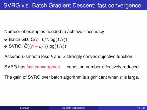
Number of examples needed to achieve ε accuracy:
Batch GD: O(n · L/λ log(1/ε))
SVRG: O((n + L/λ) log(1/ε))
Assume L-smooth loss fi and λ strongly convex objective function.
SVRG has fast convergence — condition number effectively reduced
The gain of SVRG over batch algorithm is significant when n is large.
T. Zhang Big Data Optimization 19 / 73

SVRG: variance
1
10
100
SGD: 0.0001
variance
0.00001
0.0001
0.001
0.01
0.1
1
0 50 100 150 200
variance
# epochs | #grad_comp / n
SGD: 0.0001
SGD: 0.005
SVRG: 0.005
variance 10
100
variance
0.01
0.1
1
10
0 100 200 300 400 500
variance
#epochs | #grad_comp / n
SGD:0.001
SGD:0.025
SVRG:0.025
Convex case (left): least squares on MNIST;Nonconvex case (right): neural nets on CIFAR-10.The numbers in the legends are learning rate
T. Zhang Big Data Optimization 20 / 73

SVRG: convergence
1.25
1.26
1.27
1.28
1.29
Training loss
SGD: 0.0001
SGD: 0.00025
SGD: 0.0005
1.21
1.22
1.23
1.24
1.25
0 50 100 150 200
Training loss
#epochs | #grad_comp / n
SGD: 0.001
SGD: 0.0025
SVRG:0.005
1.55
1.6
1.65
1.7
Training loss
SGD:0.001 SGD:0.0025
SGD:0.005 SGD:0.01
SVRG:0.025
1.4
1.45
1.5
1.55
0 100 200 300 400 500
Training loss
#epochs | #grad_comp / n
Convex case (left): least squares on MNIST;Nonconvex case (right): neural nets on CIFAR-10.The numbers in the legends are learning rate
T. Zhang Big Data Optimization 21 / 73

Variance Reduction using Importance Sampling(combined with SVRG)
f (w) =1n
n∑i=1
fi(w).
Li : smoothness param of fi(w); λ: strong convexity param of f (w)
Number of examples needed to achieve ε accuracy:With uniform sampling:
O((n + L/λ) log(1/ε)),
where L = maxi Li
With importance sampling:
O((n + L/λ) log(1/ε)),
where L = n−1∑ni=1 Li
T. Zhang Big Data Optimization 22 / 73
Outline
Background:big data optimization in machine learning: special structure
Single machine optimizationstochastic gradient (1st order) versus batch gradient: pros and consalgorithm 1: SVRG (Stochastic variance reduced gradient)algorithm 2: SAGA (Stochastic Average Gradient ameliore)algorithm 3: SDCA (Stochastic Dual Coordinate Ascent)algorithm 4: accelerated SDCA (with Nesterov acceleration)
Distributed optimizationalgorithm 5: accelerated minibatch SDCAalgorithm 6: DANE (Distributed Approximate NEwton-type method)behaves like 2nd order stochastic sampling
T. Zhang Big Data Optimization 23 / 73

Motivation
Solve
w∗ = arg minw
f (w) f (w) =1n
n∑i=1
fi(w).
SGD with variance reduction via SVRG:
wt = wt−1 − ηt [∇fi(wt−1)−∇fi(w) +∇f (w)]︸ ︷︷ ︸small variance
.
Compute full gradient ∇f (w) periodically at an intermediate w
How to avoid computing ∇f (w)?Answer: keeping previously calculated gradients.
T. Zhang Big Data Optimization 24 / 73

Stochastic Average Gradient ameliore: SAGA
Initialize: gi = ∇fi(w0) and g = 1n∑n
j=1 gj
SAGA update rule: randomly select i , and
wt =wt−1 − ηt [∇fi(wt−1)− gi + g]
g =g + (∇fi(wt−1)− gi)/ngi =∇fi(wt−1)
Equivalent to:
wt = wt−1 − ηt [∇fi(wt−1)−∇fi(wi) +1n
n∑j=1
∇fj(wj)]
︸ ︷︷ ︸small variance
wi = wt−1.
Compare to SVRG:
wt = wt−1 − ηt [∇fi(wt−1)−∇fi(w) +∇f (w)]︸ ︷︷ ︸small variance
.
T. Zhang Big Data Optimization 25 / 73

Variance Reduction
The gradient estimator of SAGA is unbiased:
E
∇fi(wt−1)−∇fi(wi) +1n
n∑j=1
∇fj(wj)
= ∇f (wt−1).
Since wi → w∗, we have∇fi(wt−1)−∇fi(wi) +1n
n∑j=1
∇fj(wj)
→ 0.
Therefore variance of the gradient estimator goes to zero.
T. Zhang Big Data Optimization 26 / 73

Theory of SAGA
Similar to SVRG, we have fast convergence for SAGA.Number of examples needed to achieve ε accuracy:
Batch GD: O(n · L/λ log(1/ε))
SVRG: O((n + L/λ) log(1/ε))
SAGA: O((n + L/λ) log(1/ε))
Assume L-smooth loss fi and λ strongly convex objective function.
T. Zhang Big Data Optimization 27 / 73

Outline
Background:big data optimization in machine learning: special structure
Single machine optimizationstochastic gradient (1st order) versus batch gradient: pros and consalgorithm 1: SVRG (Stochastic variance reduced gradient)algorithm 2: SAGA (Stochastic Average Gradient ameliore)algorithm 3: SDCA (Stochastic Dual Coordinate Ascent)algorithm 4: accelerated SDCA (with Nesterov acceleration)
Distributed optimizationalgorithm 5: accelerated minibatch SDCAalgorithm 6: DANE (Distributed Approximate NEwton-type method)behaves like 2nd order stochastic sampling
T. Zhang Big Data Optimization 28 / 73
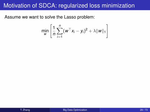
Motivation of SDCA: regularized loss minimization
Assume we want to solve the Lasso problem:
minw
[1n
n∑i=1
(w>xi − yi)2 + λ‖w‖1
]
or the ridge regression problem:
minw
1n
n∑i=1
(w>xi − yi)2
︸ ︷︷ ︸loss
+λ
2‖w‖22︸ ︷︷ ︸
regularization
Goal: solve regularized loss minimization problems as fast as we can.
solution: proximal Stochastic Dual Coordinate Ascent (Prox-SDCA).can show: fast convergence of SDCA.
T. Zhang Big Data Optimization 29 / 73
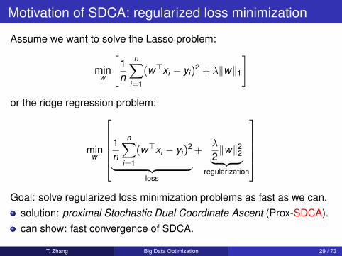

Loss Minimization with L2 Regularization
minw
P(w) :=
[1n
n∑i=1
φi(w>xi) +λ
2‖w‖2
].
Examples:φi(z) Lipschitz smooth
SVM max0,1− yiz 3 7
Logistic regression log(1 + exp(−yiz)) 3 3
Abs-loss regression |z − yi | 3 7
Square-loss regression (z − yi)2 7 3
T. Zhang Big Data Optimization 30 / 73

Loss Minimization with L2 Regularization
minw
P(w) :=
[1n
n∑i=1
φi(w>xi) +λ
2‖w‖2
].
Examples:φi(z) Lipschitz smooth
SVM max0,1− yiz 3 7
Logistic regression log(1 + exp(−yiz)) 3 3
Abs-loss regression |z − yi | 3 7
Square-loss regression (z − yi)2 7 3
T. Zhang Big Data Optimization 30 / 73

Dual Formulation
Primal problem:
w∗ = arg minw
P(w) :=
[1n
n∑i=1
φi(w>xi) +λ
2‖w‖2
]
Dual problem:
α∗ = maxα∈Rn
D(α) :=
1n
n∑i=1
−φ∗i (−αi)−λ
2
∥∥∥∥∥ 1λn
n∑i=1
αixi
∥∥∥∥∥2 ,
and the convex conjugate (dual) is defined as:
φ∗i (a) = supz
(az − φi(z)).
T. Zhang Big Data Optimization 31 / 73

Relationship of Primal and Dual Solutions
Weak duality: P(w) ≥ D(α) for all w and αStrong duality: P(w∗) = D(α∗) with the relationship
w∗ =1λn
n∑i=1
α∗,i · xi , α∗ i = −φ′i(w>∗ xi).
Duality gap: for any w and α:
P(w)− D(α)︸ ︷︷ ︸duality gap
≥ P(w)− P(w∗)︸ ︷︷ ︸primal sub-optimality
.
T. Zhang Big Data Optimization 32 / 73

Example: Linear Support Vector Machine
Primal formulation:
P(w) =1n
n∑i=1
max(0,1− w>xiyi) +λ
2‖w‖22
Dual formulation:
D(α) =1n
n∑i=1
αiyi −1
2λn2
∥∥∥∥∥n∑
i=1
αixiyi
∥∥∥∥∥2
2
, αiyi ∈ [0,1].
Relationship:
w∗ =1λn
n∑i=1
α∗,ixi
T. Zhang Big Data Optimization 33 / 73
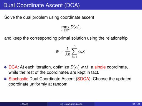
Dual Coordinate Ascent (DCA)
Solve the dual problem using coordinate ascent
maxα∈Rn
D(α),
and keep the corresponding primal solution using the relationship
w =1λn
n∑i=1
αixi .
DCA: At each iteration, optimize D(α) w.r.t. a single coordinate,while the rest of the coordinates are kept in tact.Stochastic Dual Coordinate Ascent (SDCA): Choose the updatedcoordinate uniformly at random
SMO (John Platt), Liblinear (Hsieh et al) etc implemented DCA.
T. Zhang Big Data Optimization 34 / 73
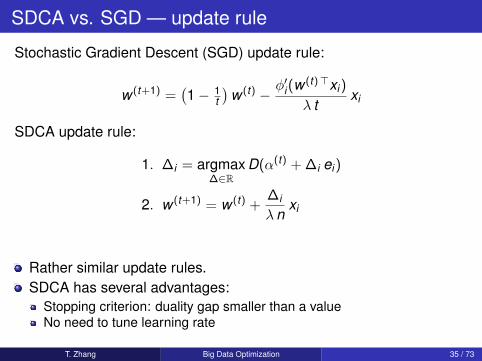
SDCA vs. SGD — update rule
Stochastic Gradient Descent (SGD) update rule:
w (t+1) =(1− 1
t
)w (t) −
φ′i(w(t)>xi)
λ txi
SDCA update rule:
1. ∆i = argmax∆∈R
D(α(t) + ∆i ei)
2. w (t+1) = w (t) +∆i
λnxi
Rather similar update rules.SDCA has several advantages:
Stopping criterion: duality gap smaller than a valueNo need to tune learning rate
T. Zhang Big Data Optimization 35 / 73

SDCA vs. SGD — update rule — Example
SVM with the hinge loss: φi(w) = max0,1− yiw>xi
SGD update rule:
w (t+1) =(1− 1
t
)w (t) −
1[yi x>i w (t) < 1]
λ txi
SDCA update rule:
1. ∆i = yi max
(0,min
(1,
1− yi x>i w (t−1)
‖xi‖22/(λn)+ yi α
(t−1)i
))− α(t−1)
i
1. α(t+1) = α(t) + ∆i ei
2. w (t+1) = w (t) +∆i
λnxi
T. Zhang Big Data Optimization 36 / 73

SDCA vs. SGD — experimental observations
On CCAT dataset, λ = 10−6, smoothed loss
5 10 15 20 2510
−6
10−5
10−4
10−3
10−2
10−1
100
SDCA
SDCA−Perm
SGD
The convergence of SDCA is shockingly fast! How to explain this?
T. Zhang Big Data Optimization 37 / 73

SDCA vs. SGD — experimental observations
On CCAT dataset, λ = 10−6, smoothed loss
5 10 15 20 2510
−6
10−5
10−4
10−3
10−2
10−1
100
SDCA
SDCA−Perm
SGD
The convergence of SDCA is shockingly fast! How to explain this?
T. Zhang Big Data Optimization 37 / 73

SDCA vs. SGD — experimental observations
On CCAT dataset, λ = 10−5, hinge-loss
5 10 15 20 25 30 3510
−6
10−5
10−4
10−3
10−2
10−1
100
SDCA
SDCA−Perm
SGD
How to understand the convergence behavior?
T. Zhang Big Data Optimization 38 / 73

Derivation of SDCA I
Consider the following optimization problem
w∗ = arg minw
f (w) f (w) = n−1n∑
i=1
φi(w) + 0.5λw>w .
The optimal condition is
n−1n∑
i=1
∇φi(w∗) + λw∗ = 0.
We have dual representation:
w∗ =n∑
i=1
α∗i α∗i = − 1λn∇φi(w∗)
T. Zhang Big Data Optimization 39 / 73

Derivation of SDCA IIIf we maintain a relationship: w =
∑ni=1 αi , then SGD rule
wt = wt−1 − η∇φi(wt−1)− ηλwt−1︸ ︷︷ ︸large variance
.
property E [wt |wt−1] = wt−1 −∇f (w)
The dual representation of SGD rule is
αt ,j = (1− ηλ)αt−1,j − η∇φi(wt−1)δi,j .
T. Zhang Big Data Optimization 40 / 73

Derivation of SDCA III
The alternative SDCA rule is to replace −ηλwt−1 by −ηλnαi :primal update is
wt = wt−1 − η(∇φi(wt−1) + λnαi)︸ ︷︷ ︸small variance
.
and the dual update is
αt ,j = αt−1,j − η(∇φi(wt−1) + λnαi)δi,j .
It is unbiased: E [wt |wt−1] = wt−1 −∇f (w)
T. Zhang Big Data Optimization 41 / 73

Benefit of SDCA
Variance reduction effect: as w → w∗ and α→ α∗,
∇φi(wt−1) + λnαi → 0,
thus the stochastic variance goes to zero.
Fast convergence rate result:
Ef (wt )− f (w∗) = O(µk ),
where µ = 1−O(λn/(1 + λn)).Convergence rate is fast even when λ = O(1/n).Better than batch method
T. Zhang Big Data Optimization 42 / 73
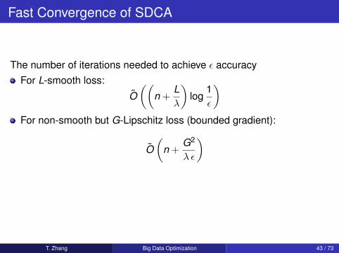
Fast Convergence of SDCA
The number of iterations needed to achieve ε accuracyFor L-smooth loss:
O((
n +Lλ
)log
1ε
)For non-smooth but G-Lipschitz loss (bounded gradient):
O(
n +G2
λ ε
)
Similar to that of SVRG; and effective when n is large
T. Zhang Big Data Optimization 43 / 73

Fast Convergence of SDCA
The number of iterations needed to achieve ε accuracyFor L-smooth loss:
O((
n +Lλ
)log
1ε
)For non-smooth but G-Lipschitz loss (bounded gradient):
O(
n +G2
λ ε
)
Similar to that of SVRG; and effective when n is large
T. Zhang Big Data Optimization 43 / 73

SDCA vs. DCA — Randomization is Crucial!
On CCAT dataset, λ = 10−4, smoothed hinge-loss
0 2 4 6 8 10 12 14 16 1810
−6
10−5
10−4
10−3
10−2
10−1
100
SDCADCA−Cyclic
SDCA−PermBound
Randomization is crucial!
T. Zhang Big Data Optimization 44 / 73

SDCA vs. DCA — Randomization is Crucial!
On CCAT dataset, λ = 10−4, smoothed hinge-loss
0 2 4 6 8 10 12 14 16 1810
−6
10−5
10−4
10−3
10−2
10−1
100
SDCADCA−Cyclic
SDCA−PermBound
Randomization is crucial!
T. Zhang Big Data Optimization 44 / 73

Proximal SDCA for General Regularizer
Want to solve:
minw
P(w) :=
[1n
n∑i=1
φi(X>i w) + λg(w)
],
where Xi are matrices; g(·) is strongly convex.Examples:
Multi-class logistic loss
φi(X>i w) = lnK∑`=1
exp(w>Xi,`)− w>Xi,yi .
L1 − L2 regularization
g(w) =12‖w‖22 +
σ
λ‖w‖1
T. Zhang Big Data Optimization 45 / 73

Dual Formulation
Primal:
minw
P(w) :=
[1n
n∑i=1
φi(X>i w) + λg(w)
],
Dual:
maxα
D(α) :=
[1n
n∑i=1
−φ∗i (−αi)− λg∗(
1λn
n∑i=1
Xiαi
)]
with the relationship
w = ∇g∗(
1λn
n∑i=1
Xiαi
).
Prox-SDCA: extension of SDCA for arbitrarily strongly convex g(w).
T. Zhang Big Data Optimization 46 / 73

Prox-SDCA
Dual:
maxα
D(α) :=
[1n
n∑i=1
−φ∗i (−αi)− λg∗(v)
], v =
1λn
n∑i=1
Xiαi .
Assume g(w) is strongly convex in norm ‖ · ‖P with dual norm ‖ · ‖D.
For each α, and the corresponding v and w , define prox-dual
Dα(∆α) =
[1n
n∑i=1
−φ∗i (−(αi + ∆αi))
−λ
g∗(v) +∇g∗(v)>1λn
n∑i=1
Xi∆αi +12
∥∥∥∥∥ 1λn
n∑i=1
Xi∆αi
∥∥∥∥∥2
D︸ ︷︷ ︸upper bound of g∗(·)
Prox-SDCA: randomly pick i and update ∆αi by maximizing Dα(·).
T. Zhang Big Data Optimization 47 / 73

Prox-SDCA
Dual:
maxα
D(α) :=
[1n
n∑i=1
−φ∗i (−αi)− λg∗(v)
], v =
1λn
n∑i=1
Xiαi .
Assume g(w) is strongly convex in norm ‖ · ‖P with dual norm ‖ · ‖D.For each α, and the corresponding v and w , define prox-dual
Dα(∆α) =
[1n
n∑i=1
−φ∗i (−(αi + ∆αi))
−λ
g∗(v) +∇g∗(v)>1λn
n∑i=1
Xi∆αi +12
∥∥∥∥∥ 1λn
n∑i=1
Xi∆αi
∥∥∥∥∥2
D︸ ︷︷ ︸upper bound of g∗(·)
Prox-SDCA: randomly pick i and update ∆αi by maximizing Dα(·).
T. Zhang Big Data Optimization 47 / 73
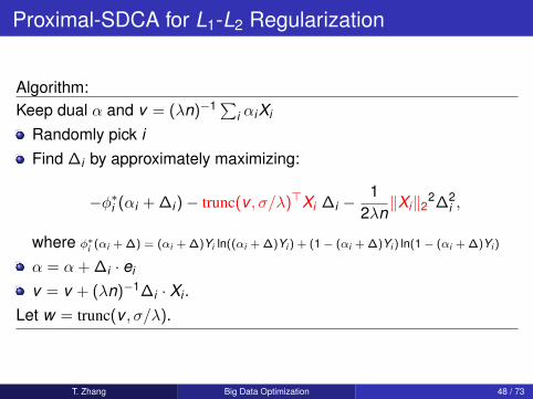
Proximal-SDCA for L1-L2 Regularization
Algorithm:Keep dual α and v = (λn)−1∑
i αiXi
Randomly pick iFind ∆i by approximately maximizing:
−φ∗i (αi + ∆i)− trunc(v , σ/λ)>Xi ∆i −1
2λn‖Xi‖22∆2
i ,
where φ∗i (αi + ∆) = (αi + ∆)Yi ln((αi + ∆)Yi ) + (1− (αi + ∆)Yi ) ln(1− (αi + ∆)Yi )
α = α + ∆i · ei
v = v + (λn)−1∆i · Xi .Let w = trunc(v , σ/λ).
T. Zhang Big Data Optimization 48 / 73

Solving L1 with Smooth Loss
Want to solve L1 regularization to accuracy ε with smooth φi :
1n
n∑i=1
φi(w) + σ‖w‖1.
Apply Prox-SDCA with extra term 0.5λ‖w‖22, where λ = O(ε):
number of iterations needed by prox-SDCA is O(n + 1/ε).
Compare to (number of examples needed to go through):Dual Averaging SGD (Xiao): O(1/ε2).FISTA (Nesterov’s batch accelerated proximal gradient): O(n/
√ε).
Prox-SDCA wins in the statistically interesting regime: ε > Ω(1/n2)
Can design accelerated prox-SDCA always superior to FISTA
T. Zhang Big Data Optimization 49 / 73

Outline
Background:big data optimization in machine learning: special structure
Single machine optimizationstochastic gradient (1st order) versus batch gradient: pros and consalgorithm 1: SVRG (Stochastic variance reduced gradient)algorithm 2: SAGA (Stochastic Average Gradient ameliore)algorithm 3: SDCA (Stochastic Dual Coordinate Ascent)algorithm 4: accelerated SDCA (with Nesterov acceleration)
Distributed optimizationalgorithm 5: accelerated minibatch SDCAalgorithm 6: DANE (Distributed Approximate NEwton-type method)behaves like 2nd order stochastic sampling
T. Zhang Big Data Optimization 50 / 73

Accelerated Prox-SDCA
Solving:
P(w) :=1n
n∑i=1
φi(X>i w) + λg(w)
Convergence rate of Prox-SDCA depends on O(1/λ)
Inferior to acceleration when λ is very small O(1/n), which hasO(1/
√λ) dependency
Inner-outer Iteration Accelerated Prox-SDCAPick a suitable κ = Θ(1/n) and βFor t = 2,3 . . . (outer iter)
Let gt (w) = λg(w) + 0.5κ‖w − y t−1‖22 (κ-strongly convex)
Let Pt (w) = P(w)− λg(w) + gt (w) (redefine P(·) – κ strongly convex)Approximately solve Pt (w) for (w (t), α(t)) with prox-SDCA (inner iter)Let y (t) = w (t) + β(w (t) − w (t−1)) (acceleration)
T. Zhang Big Data Optimization 51 / 73

Performance Comparisons
Problem Algorithm Runtime
SVMSGD 1
λε
AGD (Nesterov) n√
1λ ε
Acc-Prox-SDCA(
n + min 1λ ε ,√
nλε)
Lasso
SGD and variants dε2
Stochastic Coordinate Descent nε
FISTA n√
1ε
Acc-Prox-SDCA(
n + min 1ε ,√
nε )
Ridge Regression
SGD, SDCA(n + 1
λ
)AGD n
√1λ
Acc-Prox-SDCA(
n + min 1λ ,√
nλ)
T. Zhang Big Data Optimization 52 / 73

Experiments of L1-L2 regularization
Smoothed hinge loss +λ
2‖w‖22 + σ‖w‖1
on CCAT datasaet with σ = 10−5
0 20 40 60 80 100
0.1
0.2
0.3
0.4
0.5 AccProxSDCAProxSDCA
FISTA
0 20 40 60 80 100
0.1
0.2
0.3
0.4
0.5 AccProxSDCAProxSDCA
FISTA
λ = 10−7 λ = 10−9
T. Zhang Big Data Optimization 53 / 73
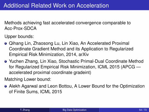
Additional Related Work on Acceleration
Methods achieving fast accelerated convergence comparable toAcc-Prox-SDCA
Upper bounds:Qihang Lin, Zhaosong Lu, Lin Xiao, An Accelerated ProximalCoordinate Gradient Method and its Application to RegularizedEmpirical Risk Minimization, 2014, arXivYuchen Zhang, Lin Xiao, Stochastic Primal-Dual Coordinate Methodfor Regularized Empirical Risk Minimization, ICML 2015 (APCG —accelerated proximal coordinate gradeint)
Matching Lower bound:Alekh Agarwal and Leon Bottou, A Lower Bound for the Optimizationof Finite Sums, ICML 2015
T. Zhang Big Data Optimization 54 / 73

Distributed Computing: Distribution Schemes
Distribute data (data parallelism)all machines have the same parameterseach machine has a different set of data
Distribute features (model parallelism)all machines have the same dataeach machine has a different set of parameters
Distribute data and features (data & model parallelism)each machine has a different set of dataeach machine has a different set of parameters
T. Zhang Big Data Optimization 55 / 73
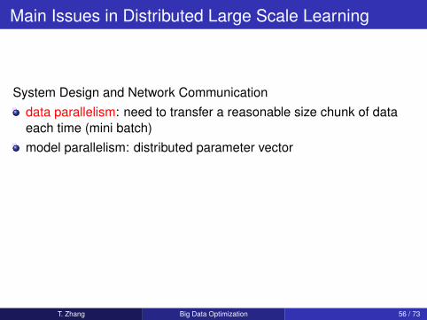
Main Issues in Distributed Large Scale Learning
System Design and Network Communicationdata parallelism: need to transfer a reasonable size chunk of dataeach time (mini batch)model parallelism: distributed parameter vector
Model Update Strategysynchronousasynchronous
T. Zhang Big Data Optimization 56 / 73

Outline
Background:big data optimization in machine learning: special structure
Single machine optimizationstochastic gradient (1st order) versus batch gradient: pros and consalgorithm 1: SVRG (Stochastic variance reduced gradient)algorithm 2: SAGA (Stochastic Average Gradient ameliore)algorithm 3: SDCA (Stochastic Dual Coordinate Ascent)algorithm 4: accelerated SDCA (with Nesterov acceleration)
Distributed optimizationalgorithm 5: accelerated minibatch SDCAalgorithm 6: DANE (Distributed Approximate NEwton-type method)behaves like 2nd order stochastic sampling
T. Zhang Big Data Optimization 57 / 73

MiniBatch
Vanilla SDCA (or SGD) is difficult to parallelizeSolution: use minibatch (thousands to hundreds of thousands)
Problem: simple minibatch implementation slows down convergencelimited gain for using parallel computing
Solution:use Nesterov accelerationuse second order information (e.g. approximate Newton steps)
T. Zhang Big Data Optimization 58 / 73

MiniBatch SDCA with Acceleration
Parameters scalars λ, γ and θ ∈ [0,1] ; mini-batch size mInitialize α(0)
1 = · · · = α(0)n = α(0) = 0, w (0) = 0
Iterate: for t = 1,2, . . .u(t−1) = (1− θ)w (t−1) + θα(t−1)
Randomly pick subset I ⊂ 1, . . . ,n of size m and updateα
(t)i = (1− θ)α
(t−1)i − θ∇fi(u(t−1))/(λn) for i ∈ I
α(t)j = α
(t−1)j for j /∈ I
α(t) = α(t−1) +∑
i∈I(α(t)i − α
(t−1)i )
w (t) = (1− θ)w (t−1) + θα(t)
end
Better than vanilla block SDCA, and allow large batch.
T. Zhang Big Data Optimization 59 / 73

Theory
Generally when minibatch size m increases, it is easier to parallelize,but convergence slows down
Theorem
If θ ≤ 14 min
1 ,√
γλnm , γλn , (γλn)2/3
m1/3
then after performing
t ≥ n/mθ
log
(m∆P(x (0)) + n∆D(α(0))
mε
)
iterations, we have that E [P(x (t))− D(α(t))] ≤ ε.
T. Zhang Big Data Optimization 60 / 73

Interesting Cases
The number of iterations required in several interesting regimes:Algorithm γλn = Θ(1) γλn = Θ(1/m) γλn = Θ(m)
SDCA n nm n
ASDCA n/√
m n n/m
AGD√
n√
nm√
n/m
The number of examples processed in several interesting regimes:Algorithm γλn = Θ(1) γλn = Θ(1/m) γλn = Θ(m)
SDCA n nm n
ASDCA n√
m nm n
AGD n√
n n√
nm n√
n/m
T. Zhang Big Data Optimization 61 / 73

Example
106
107
108
10−3
10−2
10−1
#processed examples
Prim
al suboptim
alit
y
m=52
m=523
m=5229
AGD
SDCA
MiniBatch SDCA with acceleration can employ large minibatch size.
T. Zhang Big Data Optimization 62 / 73

Outline
Background:big data optimization in machine learning: special structure
Single machine optimizationstochastic gradient (1st order) versus batch gradient: pros and consalgorithm 1: SVRG (Stochastic variance reduced gradient)algorithm 2: SAGA (Stochastic Average Gradient ameliore)algorithm 3: SDCA (Stochastic Dual Coordinate Ascent)algorithm 4: accelerated SDCA (with Nesterov acceleration)
Distributed optimizationalgorithm 5: accelerated minibatch SDCAalgorithm 6: DANE (Distributed Approximate NEwton-type method)behaves like 2nd order stochastic sampling
T. Zhang Big Data Optimization 63 / 73

Improvement
OSA Strategy’s advantage:machines run independentlysimple and computationally efficient; asymptotically good in theory
Disadvantage:practically inferior to training all examples on a single machine
Traditional solution in optimization: ADMM
New Idea: via 2nd order gradient samplingDistributed Approximate NEwton (DANE)
T. Zhang Big Data Optimization 64 / 73

Distribution Scheme
Assume: data distributed over machines with decomposed problem
f (w) =m∑`=1
f (`)(w).
m processorseach f (`)(w) has n/m randomly partitioned exampleseach machine holds a complete set of parameters
T. Zhang Big Data Optimization 65 / 73

DANE Algorithm
Starting with w using OSAIterate
Take w and define
f (`)(w) = f (`)(w)− (∇f (`)(w)−∇f (w))>w
on each machine solves
w (`) = arg minw
f (`)(w)
independently.Take partial average as the next w
Lead to fast convergence: O((1− ρ)`) with ρ ≈ 1
T. Zhang Big Data Optimization 66 / 73

DANE Algorithm
Starting with w using OSAIterate
Take w and define
f (`)(w) = f (`)(w)− (∇f (`)(w)−∇f (w))>w
on each machine solves
w (`) = arg minw
f (`)(w)
independently.Take partial average as the next w
Lead to fast convergence: O((1− ρ)`) with ρ ≈ 1
T. Zhang Big Data Optimization 66 / 73

Reason: Approximate Newton Step
On each machine, we solve:
minw
f (`)(w).
It can be regarded as approximate minimization of
minw
f (w) +∇f (w)>(w − w) +12
(w − w)>∇2f (`)(w)(w − w)︸ ︷︷ ︸2nd order gradient sampling from ∇2f (w)
.Approximate Newton Step with sampled approximation of Hessian
T. Zhang Big Data Optimization 67 / 73

Quadratc Loss
Newton:
w (t) = w (t−1) −
(1m
∑`
∇2f (`)
)−1
︸ ︷︷ ︸inverse Hessian
∇f (w (t−1))
DANE:
w (t) = w (t−1) −
1m
∑`
(∇2f (`) + µI
)−1
︸ ︷︷ ︸inverse Hessian on machine `
∇f (w (t−1)),
where a small µ is added to regularize the Hessian.
T. Zhang Big Data Optimization 68 / 73

Comparisons
0 5 10
0.229
0.23
0.231
t
COV1
0 5 100.04
0.05
0.06
0.07
t
ASTRO
0 5 10
0.03
0.04
0.05
0.06
t
MNIST−47
DANEADMMOSAOpt
T. Zhang Big Data Optimization 69 / 73
Summary
Optimization in machine learning: sum over data structureTraditional methods: gradient based batch algorithms
do not take advantage of special structureRecent progress: stochastic optimization with fast rate
take advantage of special structure: suitable for single machine
Distributed computing (data parallelism and synchronous update)minibatch SDCADANE (batch algorithm on each machine + synchronization)
T. Zhang Big Data Optimization 70 / 73

Other Developments
Distributed large scale computingalgorithmic side: ADMM, Asynchronous updates (Hogwild), etcsystem side: distributed vector computing
Nonconvex methodsnonconvex regularization and lossneural networks and complex models
Closer Integration of Optimization and Statistics
T. Zhang Big Data Optimization 71 / 73

References
SVRG:Rie Johnson and TZ. Accelerating Stochastic Gradient Descent usingPredictive Variance Reduction, NIPS 2013.Lin Xiao and TZ. A Proximal Stochastic Gradient Method withProgressive Variance Reduction, SIAM J. Optimization, 2014.
SAGA:Defazio and Bach and Lacoste-Julien, SAGA: A Fast IncrementalGradient Method With Support for Non-Strongly Convex CompositeObjectives, NIPS 2014.SDCA:
Shai Shalev-Shwartz and TZ. Stochastic Dual Coordinate AscentMethods for Regularized Loss Minimization, JMLR 2013.Shai Shalev-Shwartz and TZ. Accelerated Proximal Stochastic DualCoordinate Ascent for Regularized Loss Minimization, MathProgramming, 2015.Zheng Qu and Peter Richtarik and TZ. Randomized Dual CoordinateAscent with Arbitrary Sampling, arXiv, 2014.
T. Zhang Big Data Optimization 72 / 73

References (continued)
mini-batch SDCA with acceleration:Shai Shalev-Schwartz and TZ. Accelerated Mini-Batch StochasticDual Coordinate Ascent, NIPS 2013.DANE:Ohad Shamir and Nathan Srebro and TZ. Communication-EfficientDistributed Optimization using an Approximate Newton-type Method,ICML 2014.
T. Zhang Big Data Optimization 73 / 73