STOCHASTIC MODELLING OF FLEXIBLE...

Mathl. Cornput. Modelling Vol. 16, No. 3, pp. 15-34, 1992 0895-7177192 85.00 f 0.00 Printed in Great Britain. All rights reserved Copyright@ 1992 Pergamon Press plc

STOCHASTIC MODELLING OF FLEXIBLE MANUFACTUFtING SYSTEMS

N. VISWANADHAM, Y. NARAHARI

Department of Computer Science and Automation

Indian Institute of Science, Bangalore 560 012, India

T.L. JOHNSON

Control Systems Laboratory, General Electric CRD Center

P.O. Box 8, Schenectady, NY 12301, U.S.A.

(Received March 1990)

Abstract-Mathematical modelling plays a vital role in the design, planning and operation of flexible manufacturing systems (FMSs). In this paper, attention is focused on stochastic modelhng of FMSs using Markov chains, queueing networks, and stochastic Petri nets. We bring out the role of these modelling tools in FMS performance evaluation through several illustrative examples and provide a critical comparative evaluation. We also include a discussion on the modelling of deadlocks which

constitute an important source of performance degradation in fully automated FMSs.

1. INTRODUCTION

This paper presents a tutorial introduction to the important topic of stochastic modelling of flexible manufacturing systems (FM!%). In this area, three main modelling tools, namely Markov chains, queueing networks (QNs), and stochastic Petri nets (SPNs) have gained prominence in recent times. The paper focuses on these three modelling tools and presents illustrative examples to bring out the useful role stochastic models have come to play in logical analysis, performance evaluation and real-time control. We also include a discussion on the modelling and performance analysis of FM% with deadlocks, which represent an important source of performance degradation in FM%.

1.1. Flexible Manufacturing Systems

FMSs [l-4] have evoked considerable attention in recent times in the area of manufacturing automation, because of their high productivity. This technology is especially attractive for medium volume industries such as the automobile, aircraft, steel, and electronics industries. The philos- ophy of an FMS is ideally suited to today’s unpredictable market environment which demands low cost solutions providing for (a) quick product start-up, (b) adaptability, (c) responsiveness to changes in demand, and (d) the capacity to easily resurrect out-of-production designs.

An FMS can be defined [3] as a computer controlled configuration of numerically controlled machine tools and a material handling system(MHS) designed to simultaneously manufacture low to medium volumes of high quality products at low cost. The architecture of a typical FMS is constituted by

(a) versatile numerically controlled (NC) machines which can carry out a variety of machining operations,

(b) an automated MHS comprising one or more of carousels, conveyors, carts, robots, or automated guided vehicles (AGVs), to move parts and tools between machines,

(c) a hierarchical control system that coordinates the actions of the machines, the MHS, and the workpieces,

Typeset by A,#-lj$C

15

EluI 16:3-B

16 N. VISWANADHAM et al.

I

Central Computer

Figure 1. A typical FMS Architecture with Material and Information Integration.

Legend: PC: Programmable Controller; MHS: Material Handling System;

AGV: Automated Guided Vehicle; DBMS: Database Management System.

(d) a load/unload workstation through which the entry and exit of a part occurs; a fixturing station where the parts entering the system are fixtured onto pallets; inspection stations; coordinate measurement machines; and

(e) a buffer-storage in the form of local storage or central storage or both to store raw and semi-finished workpieces.

Often, an FMS is organized as a collection of flexible manufacturing cells (FMCs) which are interconnected by the automated MHS. A typical FMC comprises a few NC machines, tool mag- azines, and one or more material handling robots. The machines and the robots have individual programmable logic controllers (PLCs) and each FMC has a cell controller. All such controllers are interconnected via a local area network (LAN) to a host computer. Thus one can visualize two kinds of integration in an FMS: material integration provided by the automated MHS and information integration provided by the LAN and a database management system. Figure 1 depicts the architecture of a fully integrated FMS.

In Figure 2, we show a typical sequence of operations in an FMS. Initially, incoming raw workpieces are fixtured onto pallets at a load/unload station. These workpieces move to queues at

the workstations of FMCs via the MHS. The sequence of operations on a workpiece is given by the routing table (see, for example, Table 1) which also specifies the choice of machines for each operation of each part type. As a result, there are several alternative routes that a workpiece of a given type can take while being processed. In a well designed system, machines, conveyors, and control elements combine to achieve high productivity, maximum machine utilizations, and minimum in-process inventory. Some of the important decisions that the hierarchical controller takes in an FMS are: scheduling and dispatching (which part to introduce into the FMS next and which machine to be assigned to a part), scheduling of the MHS, tool management, system monitoring and diagnostics, and reacting to disruptions such as machine breakdowns, tool breakages and deadlocks. There are also several off-line decisions taken such as fixing the number of machines, number of AGVs, machine layout, machine grouping, batching and balancing; etc.

Mathematical modelling plays an important role in the on-line and off-line decision making involved in the design and operation of FMSs. Mathematical programming techniques, such as linear programming and integer programming, and heuristic techniques have been used in the prescriptive modelling of FMSs [5] to obtain optimal policies for design and operation. In this

ModeIIing manufacturing systems

Job Enters

I

Woil in IB

Fetch Tools

I

Machining

I- ,

17

Figure 2. Typical sequence of operations in an FM.9

Legend: IB: Input Buffer; OB: Output Buffer; MC: Machine Center.

Table 1. Routing Table for an FMS with 5-machines Ml, M2, M3, M4 and M5; and

three part types pl, p2, and p3.

ri

paper, we are concerned with the use of analytical evaluative models, such as Markov chains, queueing networks (QNs) and stochastic Petri nets (SPNs) in the design and operation of FMSs.

1.2. Organization of the Paper

In the next section, we present an FMS as a discrete event dynamical system and give a brief overview of FMS models considered in the literature.

Sections 3, 4, and 5 are devoted to a detailed discussion of Markov models, QN models, and SPN models respectively. In each section, we present an illustrative example to bring out the special features of each modelling tool. We also provide pointers to relevant research papers. To understand the models presented in these sections, the reader may have to refer to relevant books such as the ones by Trivedi [6] and Marasn et al. [7].


In Section 6, we consider the specific issue of the modelling of deadlocks in FMSs. We present an illustrative example using SPNs and discuss performance evaluation of FMSs with deadlocks. We conclude the paper with certain observations on future research in the important area of stochastic modelling of FMSs.

2. FMS MODELLING

An FMS can be described as a discrete event dynamical system [4,8] because changes in the system state are caused by the occurrence of events at discrete instants of time instead of completely described by partial or ordinary differential equations, as in the case of continuous variable dynamical systems. Examples of discrete events in an FMS are: entry/exit of a part, starting/finishing of a part transfer by a robot, starting/finishing of processing by a machine, a robot failure, and a machine breakdown. The number of such activities in a typical FMS is large and there are numerous interactions involving these activities. Further, these interactions exhibit concurrency, contention for resources, synchronization, and randomness. The activities are concurrent because machines and conveyors could be busy at the same time. There is a limited number of resources such as machines, tools, pallets, buffers, robots, conveyors, etc. and this causes contention for these resources and synchronization constraints. Machine failures, tool breakages, and unanticipated breakdowns occur at random points of time and this introduces randomness in activities. These interactions might also lend to a deadlocked state, in which the system is crippled and produces no output. Any effective model of an FMS should therefore capture the above characteristics.

The need for and the role of mathematical models in FMSs has been clearly brought out by Buzacott [9], Suri [5,10], and by Buzacott and Yao [ll]. FMS models can be used in a variety of ways such as in logical analysis, performance prediction, optimization, control, and for gaining insight into the system.

There are two basic types of models of discrete event dynamical systems and hence FMSs: qualitative models and quantitative models. Qualitative models such as Petri nets [12], finite state machines [13], and general algebraic discrete event models [14] are useful for investigating logical aspects of FMS behavior such as boundedness, fairness, absence/existence of deadlocks, mutual exclusion of resources, and correctness of control logic. Quantitative models are basically stochastic models that address quantitative issues of performance such as production rate of parts, manufacturing lead times, queueing characteristics, machine/robot/AGV utilizations, and reliability. According to Buzacott [9], th ere are three basic types of quantitative modelling tools: simulation models, analytical models, and hybrid models. We now give a brief review of these three types of quantitative models.

Simulation models can be used to construct a detailed representation of the system operation, generally using simulation languages such as GPSS, SIMSCRIPT, SIMULA, or SLAM. Many simulation models have been developed in industry as design aids; for example, see references [15-171. A simulation model enables a detailed representation of the characteristics of jobs, machine behaviour, flow of parts, and job routing, and complex control and sequencing rules. Thus, predictions of performance made by the model are potentially very accurate. This ability of simulation models to capture the complexity of the system makes it a very expensive tool computationally, because the simulation run can be lengthy. Also, the time to develop and adequately validate a detailed simulation model can be substantial.

Compared to simulation, analytical models of an FMS cannot capture all the details of the system. It is necessary to decide how much detail to include because too much makes the model intractable and too little makes the model unrealistic. Once a solution of an analytical model has been developed, it can be subjected to the full power of tests of mathematical correctness and precise statements can be made about the validity of the solution for the given assumptions. The process of model development and solution leads to new insight into the system and suggests ways in which assumptions might be relaxed. This in turn can lead to new ideas about how the system should be operated and controlled.

A third approach to FMS modelling uses a hybrid scheme in which simulation and analytical models are combined. Here there are two variants. In the first scheme, the modelling approach follows the framework of an analytical model but for some parts, where analysis is difficult or

Modelling manufacturing systems 19

impossible, a simulation submodel is constructed. From the results of simulation, an equivalent component for an analytical model is developed and the integrated analytical model is solved. See, for example, reference [18]. The other hybrid approach, called perturbation analysis [19,20] begins with the results of a simulation model. Using analytical techniques, the effect of a perturbation in the value of a parameter is found. Thus it is not necessary to repeat simulation runs to carry out parametric analysis. In this paper, we are concerned with analytical models only. We do not consider simulation and hybrid models.

3. MARKOV MODELS

In this section, we present Markovian modelling of FM%. Markov and semi-Markov processes are an important subclass of stochastic processes, which constitute the basis of performance evaluation using any analytical tool. The following are the advantages of Markov models. First, the data to be collected can be explained easily, since each element of a Markov transition matrix can be thought of as the relative frequency with which a transition occurs from one state to another. Second, the computations involve well-known and easily implemented matrix operations. Finally, the quantities computed from a Markov analysis can be easily interpreted. The major disadvantages of Markov analysis are:

(1) when the size of the physical system grows, the number of states in the Markov chain grows exponentially and this makes Markov analysis expensive;

(2) with increase, in the number and complexity of interactions in the physical system, it becomes difficult to visualize the Markov chain states and the transitions among the states;

(3) existence of two or more time scales lead to increased computational difficulties.

In the sequel of this section, we shall illustrate the construction of Markov models and discuss performance evaluation using these models.

3.1. Markov Model of a Central Server FMS

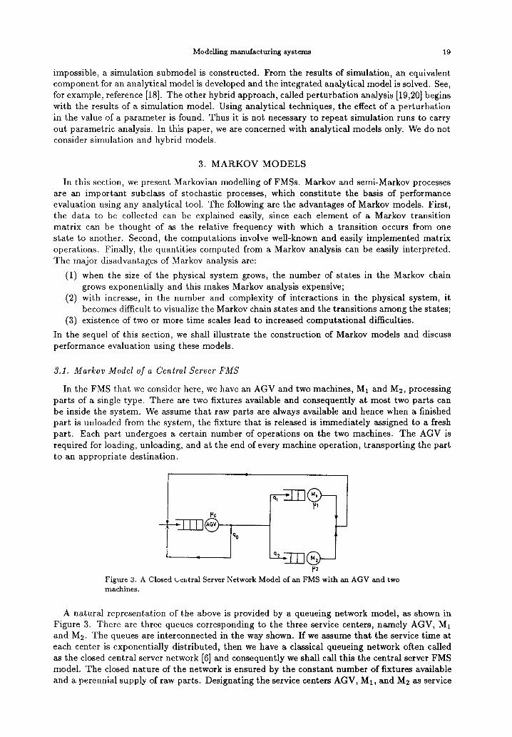
In the FMS that we consider here, we have an AGV and two machines, Mi and Mz, processing parts of a single type. There are two fixtures available and consequently at most two parts can be inside the system. We assume that raw parts are always available and hence when a finished part is unloaded from the system, the fixture that is released is immediately assigned to a fresh part. Each part undergoes a certain number of operations on the two machines. The AGV is required for loading, unloading, and at the end of every machine operation, transporting the part to an appropriate destination.

Figure 3. A Closed Leutral Server Network Model of an FMS with an AGV and two machines.

A natural representation of the above is provided by a queueing network model, as shown in Figure 3. There are three queues corresponding to the three service centers, namely AGV, Mi and Mz. The queues are interconnected in the way shown. If we assume that the service time at each center is exponentially distributed, then we have a classical queueing network often called as the closed central server network [6] and consequently we shall call this the central server FMS model. The closed nature of the network is ensured by the constant number of fixtures available and a perennial supply of raw parts. Designating the service centers AGV, Ml, and M;! as service


9, PO

Figure 4. State transition diagram of the Markov chain representing the FMS.

Table 2. Transition rate matrix of the Markov chain model of the central server FMS.

1 2 3 4 5 6

1 -h + P2)

q:;,o

P2 0 0 0

2 91 PO -(l - - P2 0 P2 QZPO 0

3 Q2 PO 0 -(l - qo)fio - Pl

4 0 q2Po 91 PO

5 0 P2 0 0 -/J2 0

6 0 0 PI 0 0 -Pl

centers 0, 1, and 2 respectively, the routing matrix would be given by

[ Qo 1 1 Ql 0 0 Q2 0 0 1 .

The choice of the routing probabilities qo, ql, and q2 will depend on the physics of processing. In this system, a fresh part is fixtured immediately after loading and is defixtured just before unloading. The released fixture is used for fixturing another fresh part. Since new parts are always available, the exit of a finished part always leads to the entry of a newly fixtured part. Thus the arc labelled by qo signals the exit of a finished part as well as the entry of a fresh part. Intuitively, it can be seen that (l/qc) is the average number of times the AGV is required to transport a typical part inside the system. Also (ql/qo) and (qz/qo) give the average numbers of times a typical part is processed by Mi and Ma, respectively, before the part leaves the system.

Since the service times at all the nodes in the queueing network model of Figure 3 are exponentially distributed, the underlying stochastic process is a continuous time Markov chain. Thus, by enumerating the set of all states, one can obtain a Markov chain representation for the above FMS. If the number of fixtures is two, there are exactly six states in this Markov chain, as shown below:

State 1: Ml and M-J processing one part each (only AGV free) State 2: M2 processing a part and AGV transporting the other part (only Mi free) State 3: Ml processing a part and AGV transporting the other part (only MS free) State 4: AGV transporting a part and the other part waiting for the AGV (Mi and M2 both

free) State 5: M7, processing a part and the other part waiting for M2 (AGV and Ml both free) State 6: Mi processing a part and the other part waiting for Mi (AGV and M2 both free).

The transitions among these states and the corresponding transition rates are shown in Figure 4. The transition rate matrix Q of the Markov chain model is shown in Table 2.


Since this Markov chain is finite and irreducible, it is ergodic. If II = (?ri, 7r2,7rz, 7r.+, 7r5, ~6) is the vector of steady state probabilities of the above Markov chain, then by the standard solution to the Kolmorgorov differential equations [6], it is known that

IIQ=O and kni=l. i=l

Ergodicity of the above Markov chain ensures that a unique solution exists for the above set of equations, and we can compute desired performance measures from these probabilities, as shown below:

Utilization of AGV = sum of the steady state probabilities of

all states in which AGV is busy

= r2 + r3 + T4

Similarly,

Utilization of Mi = ?ri + 773 + ?r6

Utilization of M2 = ~1 + ~2 + 7r5

Expected number of parts in the

-AGV subsystem = AZ + 7rs + 2~~ -Ml subsystem = ~1 + 7r3 + ?h6

-M2 subsystem = ~1 + 7r2 + 2~s.

Other performance measures can be similarly obtained.

3.2. Review of Markov Models

In the above example, let us say we increase the number of fixtures to 3. That is, there are now three jobs circulating inside the network. In this case, we can say with some difficulty that the number of states in the resulting Markov chain is 10. If we further increase the number

of fixtures, two things happen. First, the complexity of the Markov chain grows and its construction is no longer trivial. Second, the number of states in the Markov chain rises rapidly and makes computation of steady state probabilities and performance measures very expensive. Other changes in the system, such as increasing the number of AGVs or machines or both, also lead to the same complications. Note, however, that changes in routing probabilities or service rates or both will only change the transition rate matrix and leave the state space unaffected. The first of the above limitations can be effectively overcome by stochastic Petri nets which enable automatic generation of state space and transition rate matrix, using an elegant graphical representation and precise rules for dynamic evaluation. The second limitation is completely avoided by the queueing networks which do not at all generate the state space or transition rate matrix and instead use efficient polynomial time computational algorithms for computing performance measures directly. In fact, the above closed queueing network is one of the most efficiently solved queueing network models. For the above reasons, QNs and SPNs are almost always preferred to Markov chains. It should be noted that the underlying stochastic process is still a Markov or semi-Markov process, whether it be a QN model or an SPN model. To choose between SPNs and QNs, one has to weigh other considerations, some of which will be presented in subsequent sections.

Markov and semi-Markov models for manufacturing systems have been investigated by sev-

eral researchers: Gershwin and Berman [21], Gershwin and Schick [22], Buzacott and Shantiku- mar [23], Foster and Garcia-Diaz [24], Alam e2 al. [25], and Ammar [26]. Most of these researches are on traditional flow lines. Real-life phenomena such as blocking, starving, and machine failures have been modelled using Markov chains. Also in some cases efficient techniques have been presented for Markov chain analysis. For example, see [21,22]. Ammar [26] has included the effect of control and communication equipment in his Markov chain model. If we want to include failure times, processing times, and message communication times in the same Markov chain model, then we are confronted with stiff Markov chains [27] b ecause of large orders of magnitude difference among these times.


4. QUEUEING NETWORK MODELS

Queueing networks are by far the most popular and efficient analytical modelling tool for FMSs. An overview of QN models of FMSs can be obtained from the papers by Buzacott and Yao [28], Suri and Hildebrant [29], and Seidman et al. [30]. QN models capture dynamics, interactions, and uncertainties in an FMS in an aggregate way. The performance measures computed are average values which assume a steady-state operation of the system. QN-based models of FMSs can be broadly classified into the following three types [28]:

(1) Jackson Networks: Open queueing networks with fixed arrival rate, closed queueing networks, and restricted open queueing networks.

(2) Reversible Networks: Fixed routing model, fixed loading model, and dynamic routing model.

(3) Approximate QN models for handling non-product form features such as priorities, blocking, multiple resource holding, and synchronization.

In this section, we present a closed queueing network (C&N) model of a simple FMS to illustrate QN models.

4.1. Closed Queueing Network Models

The basic CQN model of an FMS was first developed by Solberg [31]. Since then several researchers have based their models on CQNs. The main assumptions of the model are as follows [ll]:

(1) The total number of jobs in the system is a fixed constant N, which can be viewed as the total number of fixtures or pallets available in the system. This implies that when a completed job leaves the system, a fresh job is ready and enters the system.

(2) At all stations with FCFS queueing discipline, service time distributions are exponential and all job classes must have the same service rate parameter at a station.

(3) All stations have a local storage large enough to accomodate all N jobs in the system. This prevents occurrence of blocking.

(4) Machines are always available for processing jobs. That is, there are no breakdowns and any set up or tool changing time is included in the service time.

A CQN with the above assumptions has an equilibrium distribution that is “product form”. Let 12 = (nl, 722, . . . , no) denote the state of the system where nc(i = 1, 2, . . . , M) is the number of jobs at station i. The state space of the system is the set of n such that

M

c ni = N. i=l

The steady state probability that the system is in state (nl, n2, . . . , no) is given by

where G(N) is the normalizing constant and fi(ni)(i = 1, 2, . . . , M) are simple functions of given parameters. The central problem is to compute G(N), and performance measures can be directly obtained from G(N). Details about efficient computational algorithms in this context may be obtained from [6].

The above model has been widely used for preliminary design of FMSs and for studying some of the issues in production planning, such as machine grouping [32]. Consider the FMS depicted in Figure 5. The system comprises four machines Ml, MS, Ms (tool machines) and L/U

(load/unloaded machine), and a cart moving along a rail. A buffer is also available to store those workpieces that have not yet been completely processed. The workpieces are of two types. Type one parts have a two-phase operation schedule, while type two parts need only one machining operation before leaving the FMS. The first phase on type one parts can be accomplished only


Figure 5. A simple FMS.

Table 3. Details of machining times for the FMS example.

Required Mean machining times in minutes

production Process Class ItliX number Ml M2 M3 TR L/U

1 20% 1 10 15 - 1 0.1

2 10 - 30 1 0.1

2 80% 1 - 15 - 1 0.1

2 30 1 0.1

Figure 6. A multiclass CQN model of the FMS of Figure 5.

on Ml, while the second phase can be performed either by Mz or by Ms. Type two parts can undergo their single operation on M2 or on Ms. There is a requirement to be met concerning production mix: of the total finished parts, 20% must be parts of type 1. Table 3 gives the data concerning the working schedules.

Inside the system, the workpieces are mounted on pallets for proper presentation and orienta- tion during processing. Different pallet types are needed for different part types. The available number of pallets thus constrains the number of workpieces of various types flowing through the system. In fact, this means that the number of parts of each type in the system is fixed and this leads to a CQN model.

Figure 6 shows a multiclass C&N model for the above system. The three machines Ml, M2,

and MS, the cart (TR), and the L/U station are numbered from 1 to 5 in that order. The solid lines and the dotted lines have been used in the figure to distinguish between the two classes. Routing probabilities for the QN model can be computed using the following arguments. First note that each part of type 1 uses the cart three times during its processing, whereas each part of type 2 uses the cart twice during its processing. Let Vi,, denote the visit ratio of parts of type r(~ = 1,2) to station (i = 1,2,3,4,5) and P,,, represent the fraction of times process number s(s = 1,2) is chosen to perform the machining of parts of type T(T = 1,2). It can be observed

24 N. VKWANADHAM et al.

that the following relations hold.

K,l = 1; vz,l = P1,1; b,l = P1,2;

v4,1 = 3; V&l = 1;

K,2 = 0; vi!,2 = p2,1; v3,2 = p2,2;

v4,2 = 2; V-z,2 = 1.

Given the structure of the model, these visit ratios uniquely identify the routing probabilities of the parts flowing through the network:

44,1,1 = 44,5,1 = I/3,

!74,2,1 = Pl,1/3,

44,3,1 = Pl,1/3,

44,1,2 = 0,

44,2,2 = P2,1/2,

44,3,2 = P2,2/2,

!74,5,2 = l/2,

where qi,j,r represents the probability that a part of class r moves to station j upon completion of processing at station i. The probabilities P,,, can be computed using the procedure outlined in [33] and can be shown to be

Pl,l = 0; Pl,2 = 1

P2,1 = .65; P2,2 = .35

Assuming that the queueing discipline is FCFS and that the processing times are exponentially distributed (with means as shown in Table 3), the above CQN becomes product form and can be analyzed using standard computational algorithms for closed queueing networks [6].

4.2. Review of QN Models

QN modelling of FMSs has been pursued at various institutions and there is a rich body of literature available in this area and notable contributions may be found in [34-391. QN models of FMSs have been well reviewed in the literature and the reader is referred to the excellent survey papers by Buzacott and Yao [11,28]. Techniques based exclusively on C&N models have been reviewed by Seidman, Schweitzer, and Shalev-Oren [30]. For this reason, we do not attempt a fresh review of QN models here.

Under suitable assumptions, QN models of FMSs become product-form queueing networks

(PFQNs) El d an can therefore be solved using efficient computational algorithms. However, features such as priorities, synchronization, multiple resource holding, and blocking make QN models non-product form and entail approximate techniques to be used. The use of approximate analysis for non-product form QN models for FMSs has been investigated by Suri and Hildebrant [29], Cavaille and Dubois [34], Shalev-Oren et al. [35], Kamath and Sanders [39], and several others. A useful alternative model that can be used in such situations is stochastic Petri nets, discussed in the next section.

5. STOCHASTIC PETRI NET MODELS

Among analytical techniques for modelling FMSs, timed Petri nets in general and stochastic Petri nets in particular have emerged as a major tool in recent times. The major reasons for the popularity of SPN-based models are: (a) the elegant graphical nature of the model, (b) analysis techniques that can be completely automated, (c) the power of the model in representing non-product form queueing network features such as blocking, synchronization, priorities, and multiple resource holding, and (d) the excellent recognition classical Petri nets have already gained


as models of logical behaviour of FM%. Dubois and Stecke [40] first employed Petri nets with deterministic timed transitions to model typical manufacturing systems and applied the results of Cohen e2 al. [41] to compute performance measures. However, the techniques presented by Dubois and Stecke are applicable to only FMSs with deterministic decision making and deterministic processing times and consequently cannot handle random phenomena. Stochastic Petri nets and, especially, generalized stochastic Petri nets (GSPNs) [7] are now being extensively used by various research groups as a performance modelling tool of FMSs. Notable contributions are reported in [33, 42-461. In this section, we present two illustrative examples to bring out the major aspects and advantages of performance modelling of FMSs by SPN-based models. We shall use GSPNs as the modelling tool.

5.1. Central Server FMS Model

We revisit here the example in Section 3. Recall that the system comprises an AGV and two machines (Figure 3). Figure 7 shows a GSPN model for the FMS under study. The circles in the diagram are called places and represent conditions or resources in the system. There are 10 places in the model. Their interpretation is given in Table 4. The horizontal bars ti, t3, t4, t5, t,j, t7 are called immediate transitions and represent logical changes in the system. The rectangular bars ta, ts, and tg are called exponential transitions and represent timed activities such as processing by machines and transportation by AGV. These three transitions are associated with exponential random variables with rates ~0, ~1, and ,LQ respectively. The interpretations of immediate and exponential transitions are also given in Table 4. The presence of black dots called “tokens” inside the places pz, pg, and plo indicates that the AGV is free, that a part is getting processed by Mi, and that a part is getting processed by Mz. This is the initial state or initial marking of the system (the words “state” and “marking” are used interchangeably in the sequel). Note that the immediate transitions t3, t4, and t5 are conflicting in the sense that only one of them fires at any point of time, disabling the others. The probability with which each can fire is specified by the probability distribution qo, ql, q2 defined on this set of transitions. Note that these are the routing probabilities. The transitions t3, t4 and t5 together with the associated probabilities is designated as a random switch.

The dynamic evolution of the GSPN model is governed by the firing rules for GSPN transitions. The evolution of markings and the transitions that lead to these markings are depicted in Figure 8. There are two types of markings here, namely vanishing markings and tangible markings. Vanishing markings are those in which at least one immediate transition is enabled and tangible markings are those in which only exponential transitions are enabled. The marking process of the GSPN model (the stochastic process that describes the dynamic evolution of the GSPN model) stays for zero time in vanishing markings because the firing time of each immediate transition is zero. On the other hand, the sojourn time of the marking process in the tangible markings is an exponential random variable. In Figure 8, each marking is represented by the set of places having a “token”. For example, tangible marking Ti is pzpgplo meaning that there is a token each in the places pz, pg, and ~10, and no token elsewhere. The following may be noted:

(i) There are 6 tangible markings (shown by double circles in Figure 8) and 11 vanishing markings (shown by single circles in the same figure). Tangible markings are precisely the six states enumerated in the continuous time Markov chain of Section 3. Vanishing markings are intermediate markings which lead to vanishing or tangible markings because of logical changes in the system.

(ii) The set of tangible and vanishing markings constitutes a discrete time Markov chain under an appropriate interpretation [7]. The transition probabilities are in fact shown in Figure 8, as the labels on the arcs.

(iii) By systematic elimination of vanishing markings as detailed in [7], a “reduced” embedded Markov chain comprising tangible markings alone may be obtained and will be the same as the Markov chain of Figure 4. Note that this Markov chain is the same as that we had obtained in Section 3.

The reader is referred to [7] for the procedure to compute the steady state probabilities

Tl, x2, “‘, r6 of the six tangible markings. Using these, we can compute several performance


7

Figure 7. A GSPN model of an FM!3 comprising an AGV and two machines.

Table 4. Description of the GSPN model of a simple FMS with an AGV and two

Pl : Queue of parts waiting to be transported by the AGV

P2 : AGV available

ps : AGV transporting a part

P4 : A part that has just been transported by an AGV

P5 : Parts waiting to get serviced by Ml

ps : Parts waiting to get serviced by M2

P7 : Ml available

PI3 : M2 available

ps : Ml processing a part

plo : A42 processing a part

t1 : AGV starts transporting a part

t2 : Transport of a part by AGV

t3 : Fished parts gets unloaded from the system and a fresh part

is carried into the system by the AGV

t4 : Part joins the queue for Ml

t5 : Part joins the queue for M2

t6 : iI41 starts processing a part

t7 : M2 starts processing a part

tg : Processing of a part by Mr

tg : Processing of a part by M2

tl, t3, t4, ts, t6, t7: ha’mdiate transitions

t3,t4,t5: Random switch with probabilities pe, ~1 and 172 respectively

t2, ts, ts : Exponential transitions with rates ~IJ, ~1 and ~2 respectively.

Mode&g manufacturing systems 27

p, ps p, ps "I1

7’ u bl

Figure 8. Embedded Markov chain for the GSPN model of Figure 7.

measures as shown in Section 3. The computation of the performance measures can be completely automated, unlike in the case of Markov chains.

In fact, the analysis of a GSPN model, starting with the generation of tangible and vanishing markings till the computation of performance measures, can be completely automated and this is a major consideration in using GSPNs.

5.2. Central Server FMS Model with Priorities

Consider again the central server based FMS considered above. Suppose now we change the operating rule in this system as described in the following: If a part finds both Afi and M2 free, then it is assigned to h4z (probably because MZ is faster) and if it finds both busy, the earlier probabilistic routing is used. Also if the part finds exactly one of the machines available, it is assigned to that machine. To capture the effect of the above decision rule using a queueing network, we need a mechanism to represent priorities. We shall now see how the above can be represented using a GSPN model. Figure 9 depicts such a GSPN model. pii and pi2 are two additional places and transitions tll - t15 are five additional transitions, in comparison with the GSPN model of Figure 7. There are “inhibitor arcs” in this model (Figure 9) indicated by a black dot as the end marker on the transition. For example, consider transition t10, which now fires only if there is a token in plr and there is no token in either p7 or pa. This is because of the existence of a “normal” arc from pii to tlo and inhibitor arcs from p7 and ps to tlo. Inhibitor arcs provide a mechanism to represent priorities in the system. Note that in this GSPN model, there are two random switches [ta, ta] and [t 14, t15] instead of the single random switch [ts, t4, t5] in the case of Figure 7. This is required in order to model the prioritized decision rule. Also note the changes made in the associated probabilities of these random switches.

Now, let us complicate the decision rule further, by stipulating that if a part finds both machines busy, it will be assigned to the queue with the smaller number of waiting parts. Further if the two queues comprise the same number of waiting parts, we would route based on the probabilities ql and qz. This new decision rule can be modelled by the same GSPN (Figure 9), with the “static” random switch [t 14, t15] replaced by a “dynamic” random switch, as shown below. The probabilities of firing t14 and t15 will now depend on the current marking M of the GSPN model

28 N. VISWANADHAM et a/.

Figure 9. GSPN Model representing priorities in the central server FMS.

and will be defined as under:

Prob(tl4) = 0 if M(Ps) > M(Ps)

= ql/(ql + q2) if M(P5) = M(P6)

= 1 if M(&) < M(P6)

Prob(tls) = 0 if M(&?j) > M(Ps)

= 42/(41 + 42) if M(P6) = M(P5)

= 1 if M(&) < kf(P5).

The above example shows the power and elegance of GSPNs in modelling features that cannot be easily handled using QNs and Markov chains.

5.3. Review of SPN Models

GSPNs provide a compact, graphical framework as a modelling tool. It is easy to construct and understand GSPN models and their analysis can be completely automated. In comparison to Markov chains, GSPNs offer the advantages of automatic generation of the transition rate matrix. Also, aggregated GSPN models can lead to a significant reduction in the number of states of the Markov chain. Compared to product form QNs, GSPNs are more powerful because of their ability to represent non-product form features. However, product form QNs are certainly much more efficient wherever applicable, and approximate analysis of non-product form queueing networks

Model&g manufacturing systems 29

l ml * . m2 * t -_ Un’oad - Load

I I

i

I I

r \ i . . Figure 10. A simple transfer line with two machines and an AGV.

Figure 11. A GSPN Model for the transfer line of Figure 10.

is also a good alternative to GSPNs. An excellent comparison between the relative virtues of GSPNs and product form QNs may be found in [47]. The integrated technique proposed by Balbo, Bruell, and Ghanta [48], combining the best features of product form QNs and GSPNs in the same modelling framework, should prove to be quite useful in the FMS context.

6. MODELLING OF DEADLOCKS

Deadlock is one of the major issues which has received wide attention in the context of automated manufacturing. Deadlocks [49] p re resent a highly undesirable phenomenon in resource sharing concurrent systems. A deadlock is a situation where each of a set of two or more jobs keeps waiting indefinitely for the other jobs in the set to release resources. The occurrence of a deadlock can potentially stall all production in an automated factory. In this section, we present how analytical modelling of deadlocks can be done using stochastic models.

6.1. A Simple Manufacturing Deadlock

To visualize an example of a deadlock in a manufacturing system, consider a transfer line comprising two machines, ml and m2, and an automated guided vehicle (AGV), shown in Figure 10. The AGV can carry only one part at a time. Assume that a given part undergoes the operations in the following sequence: (i) A fresh part, say p, enters the system when ml is free. (ii) After the machining by ml is complete, the AGV picks up p and delivers it to m2 if ms is free, otherwise the part waits on the AGV. (iii) When m2 finishes processing p, the AGV unloads the part from the system.


Table 5. Description of the GSPN model of Figure 11.

Places:

Pl : At least one raw part waiting for processing by Ml

pz: Ml idle

P3 : Ml processing a part

p4 : Ml waiting for AGV, after finishing processing

ps : AGV transporting a part, from Ml to Mz

P6 : AGV waiting for MS, after bringing a part to M2

P7 : M2 idle

Pa : AGV idle

pg : M2 processing a part

plo : M2 waiting for AGV, after finishing processing

~11 : AGV transporting a part from M2 to unload station

Transitions:

t1 : Ml starts processing a part

t2 : Processing of a part by Ml

t3 : AGV starts transporting a part from Ml to M2

t4 : Traveling of AGV from Ml to M-J

t5 : M2 starts processing a part

t6 : Processing of a part by M2

t7 : AGV starts transporting a part from M2 to unload station

ta : Traveling of AGV from M2 to unload station

t1, t3, ts, t7 : Immediate transitions

t2, t4, tg, tg : Exponential transitions

Figure 11 shows a GSPN model for the above system and Table 5 contains a description of the places and transitions in this model. Now, imagine the following sequence of events, starting with an initial state in which ml and m2 are both free and AGV is available: (i) A fresh part, say pl, enters the system, gets processed by ml and is delivered at m2 by the AGV; m2 starts processing pi. (ii) A second part, say p2, enters the system, gets processed by ml, is put on the AGV and transported to m2, but the part waits on the AGV since m2 is busy. (iii) A third part, ps, enters the system and gets processed by ml. Meanwhile, m2 finishes processing pl. At this stage, ml is blocked because AGV is not available; AGV will not become available unless m2 is free; ms cannot be free until AGV is available. This situation is called a deadlock and the whole system comes to a standstill as shown by the event sequence diagram in Figure 12. In the GSPN model, the firing sequence of transitions that would lead to this deadlock is ~~~~~~~~~~~~~~~~~~~~~~~~~ When the transitions fire in that sequence, we reach a marking in which none of the transitions is enabled, indicating a deadlock in the underlying FMS. Such situations can potentially occur in manufacturing systems because of limited number of resources, concurrent activities, and random nature of failures.

Now, consider two transfer lines, Tl and T2, of the type discussed above, and interconnected by a buffer. Assume that the parts processed by Tl are deposited in the buffer and T2 takes its input parts from the buffer. Now, if there occurs a deadlock of the type discussed above, in the transfer line T2, it would be a partial deadlock for the overall system. Now, Tl processes more parts and deposits them in the buffer. Once the buffer becomes full, the entire system is deadlocked. The above shows how a partial deadlock eventually leads to a (full) deadlock in the entire system. The occurrence of a deadlock or a partial deadlock can cripple the entire system and can potentially render automated operation impossible. The problem of deadlocks is therefore an important one to be tackled in FMSs.

Most studies of FMS deadlocks (see for example [12,50]) have focused on proving the existence/absence of deadlocks using Petri net models. Here, we show how a stochastic model such as a GSPN model can capture deadlocks in an FMS.

Modelling manufacturing systems

Figure 12. An event sequence diagram that shows the sequence leading to the occurrence of deadlock.

31

Figure 13. Reachability graph of the GSPN model of the transfer line.

v,,..., Vs are vanishing markings.

TI , . . . , Tlr are tangible markings.

6.2. Analysis of Deadlocks

The GSPN model of Figure 11 can be used to study the performance of the transfer line, in the presence of deadlocks. The reachability graph of this GSPN model is shown in Figure 13. There are 8 vanishing markings and 14 tangible markings in the reachability set. The vanishing markings are shown by single circles and the tangible markings by double circles. While constructing the GSPN model, we have assumed that all processing times and AGV transportation times are exponential random variables. Using this reachability graph, the following issues can be studied:

(1) The marking p1p4p6p10 corresponds to a deadlock since none of the transitions of the GSPN model is enabled in this marking. As soon as the marking process reaches this state, it would get absorbed and remain there forever. So, the marking process here is a semi-Markov process with single absorbing state. In general, there will be as many

H.24 16:3-C


absorbing states as the number of deadlocks. By doing an extensive path analysis of the reachability graph, we can enumerate the set of all transition firing sequences that lead to the deadlock. An analysis of these sequences can lead to operating rules for preventing the occurrence of deadlocks. For example, in Figure 13, we should not allow the marking process to go from V3 to Ts and from VT to I&, . This can be ensured, respectively by keeping machine ml idle when AGV is transporting a part from ml to m2 and by keeping the AGV idle when machine m2 is busy. Such operating rules may often lead to underutilization of resources and may also be difficult to formulate if the number of markings is very large. However, whenever feasible, this approach guarantees complete prevention of deadlocks.

(2) By eliminating all the vanishing markings from the above reachability graph as outlined in [7], we obtain a continuous time Markov chain with absorbing states. Using the theory of such Markov chains [6], we can evaluate the performance of an FMS in the presence of deadlocks. The performance measures of interest here would be: probability of occurrence of a particular deadlock (among several possible deadlocks), expected time to deadlock, and expected number of parts produced before the occurrence of a deadlock.

(3) If deadlock recovery mechanisms have been incorporated in the FMS, then we can again use GSPN models to capture deadlock recovery. We can then compute the FMS performance in the presence of deadlocks and the overheads caused by recovery schemes.

In summary, stochastic modelling can provide useful information about the performance of an FMS in the presence of deadlocks and also can suggest deadlock prevention schemes.

7. CONCLUSIONS

We have surveyed the principal modelling tools for FMSs and also presented, through examples, their use in the evaluation of performance of FMSs. Each tool by itself currently constitutes a large area of active research.

The research surveyed here concentrates most on analysis after a configuration has been specified. Arriving at configurations which meet a set of stated specifications is more an art than science as it stands now. Efforts for developing systematic methods of configuring FMSs for given part types, throughputs, lead time, quality and cost would be worthwhile.

As we have commented often in the text of the paper, FMSs lead to large models with varying time scales. Computational methods for solving such models in a reasonable time and effort is an issue. A time honored way of conquering largeness is through decomposition and aggregation. Systematic methods are needed which use system physical structure to naturally decompose systems and use the aggregated models for total system performance evaluation. Solutions of these models on parallel machines are slowly emerging. Tool boxes, which integrate various

performance evaluation tools, would help in managing a large number of distinct models suitable for different settings. Integrated modelling techniques, combining the best features of product form QNs and GSPNs, as in [48], also hold promise.

Blocking, deadlock, and failures are all generic issues in the FMS context. Performance evaluation of FMSs in the presence of these needs attention.

REFERENCES

1. P.G. Ranky, The Design and Operation of Flexible Manufacturing Sysiems, IFS Publications and North- Holland, (1983).

2. J. Hatvany, Editor, World Survey on CAM, Butterworths, Kent, U.K., (1983). 3. Draper Laboratory, Flexible Manufaclrring Systems Handbook, Noyes Publications, Park Ridge, New Jersey,

(1984).

4. Y.C. Ho, Editor, Dynamics of discrete event systems, Special Issue of Proceedings of the IEEE 77 (1)

(January, 1989). 5. R. Suri, An overview of evaluative models for flexible manufacturing systems, Annals of Operations Research

3, 13-21 (1985).

6. K.S. Trivedi, Probability and StaMica with Reliability, Queueing and Compuler Science Applicutiona, Prentice-Hall Inc., Englewood Cliffs, N.J., (1982).

7. M.A. Marsan, G. Balbo and G. Conte, PeTjormance Models of M?&iprocessor Systems, The MIT Press, Cambridge, Massachusetts, (1986).


8. Y.C. Ho, Performance evaluation and perturbation analysis of discrete event systems, IEEE Trans. A&o-

matic Control AC-32 (7), 563-572 (July, 1987).

9. J.A. Buzacott, Modelling manufacturing systems, Robotics and Computer Zntegraied Manufacturing 2 (l),

25-32 (1985). 10. FL Suri, Quantitative techniques for robotic system analysis, In Handbook of Industrial Robotics, (Edited

by S.Y. Nof), pp. 605-638, John Wiley & Sons, New York, (1985).

11. J.A. Buzacott and D.D. Yao, Flexible manufacturing systems: A review of analytical models, Management

Science 32 (7), 890-905 (1986). 12. Y. Narahari snd N. Viswanadham, A Petri net approach to modelling and analysis of flexible manufacturing

systems, Annals of Operations Research 3, 449-472 (1985).

13. W.M. Wonham, A control theory for discrete event systems, Systems Control Group Report #8714. (De-

cember 1987). 14. K.M. Inan and P.P. Varaiya, Algebras of discrete event models, Proceedings of the IEEE 77 (l), 24-38

(January, 1989).

15. J.P. Bevans, First choose an FMS simulator, American Machinist, 143-145 (May 1982).

16. H.A. Elmaraghy, Simulation and graphical animation of advanced manufacturing systems, Journal of Man-

ufacturing Systems 1 (l), 53-64 (1982).

17. A.S. Carrie, The role of simulation in FMS, In Flezible Manufacturing Systems: Methods and Sludiea,

(Edited by A. Kusiak), pp. 191-208, Elsevier Publishers, Amsterdam, (1986).

18. J.G. Shantikumar and R.G. Sargent, A hybrid simulation/analytic model of a computerized manufacturing

system, Proc. ZFORS Conference, Hamburg, Germany, (1981).

19. Y.C. Ho, A survey of perturbation analysis of discrete event dynamical systems, Annals of Operations

Research 3, 393-405 (1985).

20. R. Sari, Perturbation analysis: The state of the art and research issues explained via G/G/l queue, Proc.

of IEEE 77 (l), 114-137 (January 1989).

21. S.B. Gershwin and 0. Berman, Analysis of transfer lines consisting of two unreliable machines with random

processing times and finite storage buffers, AZZE Transactions 13 (l), 2-11 (March 1981).

22. S.B. Gershwin and I.C. Schick, Modelling and analysis of three-stage transfer lines with unreliable machines

and finite buffers, Operations Research 31 (2), 354-380 (Mar&-April 1983).

23. J.A. Buzacott and J.G. Shantikumar, Models for understanding flexible manufacturing systems, AZZE Trans-

actions 12 (4), 339-349 (December 1980).

24. J.W. Foster and A. Garcia-D&, Markovian models for investigating failure and repair characteristics of

production systems, ZZE Tmnsactions 15, 202-210 (1983).

25. M. Alam, D. Gupta, S.I. Ahmad and A. Raouf, Performance modelIing and evaluation of flexible manu-

facturing systems using semi-Markov approach, In Flexible Manufacturing, (Edited by A. Raouf and S.I. Ahmad), pp. 87-118, Elsevier Publishers, (1985).

26. M.H. Ammar, Performance of a two stage manufacturing system with control and communication overhead, IEEE Trans. Syslems, Man, and Cybernetics SMC-17 (4), 661-665 (July-August 1987).

27. P.J. Curtois, Decomposabilily: Q aeceing and Computer Systems Applications, Academic Press, New York,

(1987).

28. J.A. Buzacott and D.D. Yao, On queueing network models of flexible manufacturing systems, Queueing

Systems 1, 5-27 (1986).

29. R. Suri and R.R. Hildebrant, Modelling flexible manufacturing systems using mean value analysis, Journal

of Manufacturing Systems 3 (l), 27-38 (1984).

30. A. Seidman, P.J. Schweitzer and S. Shalev-Oren, Computerized closed queueing network models of flexible

manufacturing systems: A comparative evaluation, LaTge Scale Systems 12, 91-107 (1987).

31. J.J. Solberg, A mathematical model of computerized manufacturing systems, Proc. Fourth International

Conference on Prodac2ion Research, Tokyo, (1977).

32. K.E. Stecke and J.J. Solberg, The optimality of unbalancing both work-loads and machine group sizes in

closed queueing networks of multi-server queues, Operations Research 33, 882-910 (1985).

33. G. Balbo, G. Chiola, G. Franceschinis and G.M. Roet, Generalized stochastic Petri nets for performance

evaluation of FMS, PTOC. of 1987 IEEE Conference on Robotics d Automa2ion, 1013-1018 (March 1987).

34. J.B. Cavaille and D. Dubois, Heuristic methods based on mean value analysis for flexible manufacturing

systems performance evaluation, Proc. Zlst IEEE Conf. Decision d Control, pp. 1061-1065, Florida, (1982).

35. S. Shalev-Oren, A. Seidman and P.J. Schweitzer, Analysis of flexible manufacturing systems with priority

scheduling: PMVA, Annals of Operations Research 3, 115-128 (1985).

36. J.A. Buzacott and J.G. Shantikumar, On approximate queueing models of dynamic job shops, Management

Science 31, 870-887 (1985).

37. J.G. Shantikumar and J.A. Buzacott, Open queueing network models of dynamic job shops, International

Journal of Produclion Research 19, 255-266 (1981).

38. E.G. Coffman, Jr., E. Gelenbe and E.N. Gilbert, Analysis of a conveyor queueing a flexible manufacturing

system, Proc. 1986 ACM SZGMETRZCS Conf. on Measurement and Modelling of Computer Systems,

204-223 (1986).

39. M. Kamath and J.L. Sanders, Analytical methods for performance evaluation of large asynchronous auto-

matic assembly systems, Large Scale Systems 12, 143-154 (1987).

34 N. VISWANADHAM el al.

40.

41.

42.

43.

44.

45.

46.

47.

48.

49.

50.

D. Dubois and K.E. St&e, Using Petri nets to represent production processes, PTOC. of the 22nd IEEE

Conference on Decision d Control, pp. 1062-1067, San Antonio, Texae, (1983). G. Cohen, D. Dubois, J.P. Quadret and M. Viot, A linear system theoretic view of discrete event processes and its use for performance evaluation in manufacturing, IEEE TTans. Automatic Control AC-30 (3), 210-220 (March 1985). G. Bruno and P. Biglia, Performance evaluation and validation of tool handling in flexible manufacturing systems using Petri nets, PTOC. of International Workshop on Timed Petri Nets, pp. 64-71, Torino, Italy, (July 1985). N. Viswanadham and Y. Narahari, Stochastic Petri net models for performance evaluation of automated manufacturing systems, Informalion and Decision Technologies 14, 125-142 (1988). M.A. Marsan, G. Balbo, G. Chiola, and G. Conte, Generalized stochastic Petri nets revisited: Random switches and priorities, Proc. Znlernational Workshop on Petri Nets and Performance Modela, pp. 4353, Madison, Wisconsin, (August 1987). F. Archetti, E. Fagiuoli and A. Sciomachen, Computation of the makespan in a transfer line with station breakdowns using stochastic Petri nets, Compulers and Operations Research (1987). H.P. Hillion and J.M. Proth, Perfo rmance evaluation of job-shop systems using timed event graphs, IEEE

Trans. Audomatic Control AC-34 (l), 3-9 (January 1989). M.K. Vernon, J. Zahorjan and E.D. Lazowska, A comparison of performance Petri nets and queueing network models, Proc. of International Workshop on Modelling Techniques and Performance Evaluation,

pp. 181-192, AFCET, Paris, France, (March 1987). G. Balbo, S.C. Bruell and S. Ghanta, Combining queueing network end generalized stochastic Petri nets for the analysis of software blocking phenomena, IEEE Trans. Software Engineering SE-12 (4), 561-576 (April 1986). E.G. Cotian, M.J. Elphick and A. Shoshani, System deadlocks, ACM Computing Surveys 3 (2), 67-78 (June 1971). H. Alla, P. Ladet, P. Martinez and M. Silva, Modelling and validation of complex systems by coloured Petri nets: Application to FMS, In Advances in Petri Nets-f 984, Lecture Notes in Computer Science, Vol. 188, pp.15-31, Springer-Verlag, Berlin, West Germany, (1985).

STOCHASTIC MODELLING OF FLEXIBLE...

Documents

Transcript of STOCHASTIC MODELLING OF FLEXIBLE...