Stochastic Modeling Workshop — Mortality

Southeastern Actuaries Conference

Noel Harewood

November 19, 2003

2

Outline

� Overview

� Techniques for generating stochastic mortality scenarios

� Case studies: Practical applications of stochastic mortality� Case Study 1: Senior settlements� Case Study 2: COLI reinsurance� Case Study 3: Economic capital

� Closing thoughts

Overview

4

Stochastic mortality techniques can provide a heightened

degree of insight to certain types of financial analyses

� Mortality assumptions have been traditionally modeled as a deterministic process, represented by a table of death rates. This approach is simple and allows for risks to be easily replicated and compared.

� The deterministic approach, while often sufficient for most analyses, ignores two important aspects of mortality:� Mortality volatility risk (mitigated due to the law of

large numbers).� Misestimation risk (controlled by underwriting).

more . . .

5

Stochastic mortality techniques can provide a heightened

degree of insight to certain types of financial analyses (cont.)

� Additional considerations for these aspects becomes more necessary when:� The analysis has a limited number of lives at risk.� The economic consequences of death have a high

severity but low probability of occurrence, such as the case of stop loss reinsurance.

� These situations can be best dealt with by employing stochastic mortality modeling techniques.

When properly applied, stochastic mortality modeling techniques can provide useful insights into the variability in financial performance of a life insurance vehicle or transaction.

When properly applied, stochastic mortality modeling techniques can provide useful insights into the variability in financial performance of a life insurance vehicle or transaction.

Techniques for Generating Stochastic

Mortality Scenarios

7

Monte Carlo simulation is a common technique used to

generate stochastic mortality scenarios

� Monte Carlo simulations associate a sequence of random numbers with a probability distribution to explain a real-life process, system or behavior.

� The key elements of a Monte Carlo simulation include:� Random number generator� Choice of a parameterized probability distribution� Real-life interpretation of the random number generation

� A graphical representation of Monte Carlo simulation follows:

Random Number GeneratorXi = ε [0,1]

Random Number GeneratorXi = ε [0,1]

PDF (Defined Process)Yi ~ Dist(parm1, parm2,…)PDF (Defined Process)

Yi ~ Dist(parm1, parm2,…)

XiXi

Solve for Yi stXi = F(Yi; parm1, parm2,…)

Solve for Yi stXi = F(Yi; parm1, parm2,…)

more . . .

8

� Example of Monte Carlo simulation of death rates on a cohort of N policies:� N random numbers Xi are generated on the unit

interval.� The parameterized probability distribution Yi ~

Bernoulli(qx+ti).

� Yi = 1 if Xi > qx+ti (real-life interpretation: = insured

survives), 0 if Xi <= qx+ti (real-life interpretation:

insured dies).

Monte Carlo simulation is a common technique used to

generate stochastic mortality scenarios (cont.)

9

Stochastic mortality rates can also be generated using

two parameterization techniques

� Assume a single paid-up whole life contract, where the present value of future benefit cash flows is a random variable:

PVFBC = bvT

� T is the random variable for time until death, expressed as P(T<t) = tqx

� A functional form is selected for T (such as Gompertz), and parameters are fitted to experience data from using techniques such as least squares

� Once fitted, PVBCF is developed from variable transformation techniques

� Portfolio then constructed from building block type of approach

� Advantages / Disadvantages:

(-) Time consuming

(-) Complex mathematics

� Define stochastic mortality rate as a function of deterministic tabular rate:

qx1 = atqx + bt, where

qx = tabular mortality

at = random deviations around qx

bt = random shocks around atqx

� at distribution defined such that E(at) = 1,

Var(at ) = σa2

� bt distribution defined such that E(bt) = 0,

Var(at ) = σb2

� Advantages / Disadvantages:

(+) Easy to model in standard actuarial software packages

Parameterization of Individual Mortality Parameterization of Aggregated Death Rates

Case Studies

Practical Applications of Stochastic Mortality

11

There are several practical applications of stochastic

mortality being conducted in the industry today

� Senior settlements � Stochastic mortality techniques are used to help

evaluate heightened degree of mortality uncertainty surrounding senior settlements.

� COLI reinsurance� Sellers of COLI sometimes purchase stop-loss

reinsurance coverage to protect against catastrophic claims. Stochastic mortality techniques better exploit the risk profile of a treaty given the low frequency / high severity nature of the stop-loss transaction.

more . . .

12

There are several practical applications of stochastic

mortality being conducted in the industry today (cont.)

� Economic capital analysis� Actuaries evaluating economic capital on product

lines whose financials are most heavily influenced by mortality experience may decide to run projections using stochastic mortality in addition to investment scenarios.

� Tillinghast developed case studies for each of the above examples. Results of these case studies are presented on the following slides.

Case Study 1: Senior Settlements

14

A senior settlement is a transaction where ownership of a life

insurance policy is sold for an amount greater than the cash

value

� Senior settlements are bundled and sold as investments� Typically, buyers do not have an insurable interest in the

insured’s life

� Characteristics of typical senior settlement portfolios are as follows:� Lives are aged 65 and older� Each life is assessed a mortality rating (e.g., 200% of

standard)− Life expectancy is computed based on the base mortality

table and the mortality rating� Policies are for a relatively high face amount� Limited number of policies involved in transaction (50 to 1,000)

� Reinsurance that pays out the death benefit two years after estimate of life expectancy is frequently utilized

� Given the limited number of lives and the reinsurance structure,senior settlement portfolios are prime candidates for stochasticmortality analysis

15

We have analyzed a hypothetical senior

settlement portfolio

� Lives ranged in age from 65 to 85

� Lives rated from standard to 600%

� 50 lives in the portfolio

9.39.1

9.4

10.310.6

8.0

8.5

9.0

9.5

10.0

10.5

11.0

Mean Median 75th Percentile 90th Percentile 95th Percentile

Note: Life expectancy based on base mortality of 100% of SOA 1990-95 experience table, age last birthday, select and ultimate. Extra mortality was kept level in durations 5 and later. No mortality improvement was utilized

Note: Life expectancy based on base mortality of 100% of SOA 1990-95 experience table, age last birthday, select and ultimate. Extra mortality was kept level in durations 5 and later. No mortality improvement was utilized

Average Life Expectancy(Based on 1,000 Monte Carlo Simulations)

Yea

rs

16

As noted previously, reinsurance is available on senior

settlement business where death benefit is paid out

after the life expectancy plus two years

16.7 1719

2122

0

5

10

15

20

25

Mean Median 75thPercentile

90thPercentile

95thPercentile

Number of Lives Where Reinsurance is Paid(Based on 1,000 Monte Carlo Simulations)

Liv

es

Analysis demonstrates mortality volatility risk of the portfolio. However, results are based on assumed level and pattern of mortality. Assumptions that underly the assumed level and pattern of mortality include: base mortality, mortality rating, implementation of mortality rating, utilization of mortality improvement. Misestimation of any of these assumptions introduces a risk that is not provided for in the above stochastic analysis.

Analysis demonstrates mortality volatility risk of the portfolio. However, results are based on assumed level and pattern of mortality. Assumptions that underly the assumed level and pattern of mortality include: base mortality, mortality rating, implementation of mortality rating, utilization of mortality improvement. Misestimation of any of these assumptions introduces a risk that is not provided for in the above stochastic analysis.

Case Study 2: COLI Reinsurance

18

Case Study 2: COLI Reinsurance

� To protect against catastrophic claim experience, issuers of COLI sometimes enter into a stop-loss reinsurance agreement.

� Reinsurers will typically offer to cover a percentage of claims in excess of a defined threshold, in exchange for a retention charge (usually a % of AV or COIs).

� Reinsurers are faced with the following decisions when structuring the treaty:� What percentage of claims in excess of the

threshold satisfies profitability requirements?� What risk profile are they willing to accept for a

given treaty structure?more . . .

19

Case Study 2: COLI Reinsurance (cont.)

� A case study was created to analyze stop-loss reinsurance transactions:� The COLI treaty was first analyzed deterministically

using best-estimate mortality assumptions.� The treaty was then analyzed using stochastic

mortality, as follows:− An MS-Excel spreadsheet was developed that

projected cohort experience stochastically based on the Monte Carlo method.

− For each scenario of cohort experience, fund values were generated and used to calculate the reinsurance net gain or loss on the transaction

� Results of the case study follow.

20

Deterministic mortality projections do not provide the

necessary depth to evaluate treaty characteristics

� The deterministic mortality assumption applied to certificateholderswas 80% of the 83 GAM table.

� COLI product and reinsurance cash flows were projected assuming a 10, 20 and 30% quota-share percentage.

� Profitability and risk were analyzed by calculating the net present value of reinsurance cash flows, and the maximum probability of a reinsurance claim in a period:

Key Metrics from Deterministic Projection

Quota Share %

80% 83 GAM 10% 20% 30%

NPV Reinsurance Cash Flows ($ millions)

Max P (Claim) in a Projection Period

$0.8

0.0%

$1.5

0.0%

$2.3

0.0%

21

� The deterministic projection results suggest that higher quota-share percentages result in a more profitable outcome

� However, the best-estimate mortality assumptions never produce a large enough amount of certificateholder claims to force the reinsurer into a claim payment

Deterministic mortality projections do not provide the

necessary depth to evaluate treaty characteristics

(cont.)

22

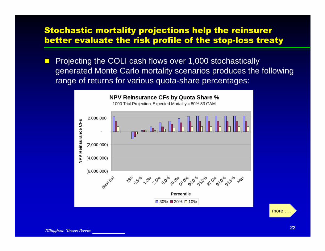
Stochastic mortality projections help the reinsurer

better evaluate the risk profile of the stop-loss treaty

� Projecting the COLI cash flows over 1,000 stochastically generated Monte Carlo mortality scenarios produces the followingrange of returns for various quota-share percentages:

NPV Reinsurance CFs by Quota Share %1000 Trial Projection, Expected Mortality = 80% 83 GAM

(6,000,000)

(4,000,000)

(2,000,000)

-

2,000,000

Best E

st

Min0.5

%1.0

%2.5

%5.0

%10

.0%50

.0%90

.0%95

.0%97

.5%99

.0%99

.5% Max

Percentile

NP

V R

ein

sura

nce

CF

s

30% 20% 10%

more . . .

23

� The best-estimate projection looks more like a best case scenario.

� The reinsurer can now not only evaluate whether the average returns are sufficient, but can also evaluate the treaty’s risk profile.

Stochastic mortality projections help the reinsurer

better evaluate the risk profile of the stop-loss treaty

(cont.)

24

Modifying the expected mortality assumption used to

develop the Monte Carlo scenarios adds further insight

(cont.)

� The reinsurer may also want to know the sensitivity of the projected reinsurance cash flows to changes in the underlying expected mortality assumption:

NPV Reinsurance CFs by Expected Mortality %1000 Trial Projection, Quota Share % = 20%

(6,000,000)

(4,000,000)

(2,000,000)

-

2,000,000

Best E

st

Min0.5

%1.0

%2.5

%5.0

%10

.0%50

.0%90

.0%95

.0%97

.5%99

.0%99

.5% Max

Percentile

NP

V R

ein

sura

nce

CF

s

70% 83GAM 80% 83GAM 90% 83GAM

25

Modifying the expected mortality assumption used to

develop the Monte Carlo scenarios adds further insight

(cont.

� The profitability and risk profile of the treaty change dramatically when introducing a 10 percentage point change in expected mortality.

� This degree of mortality sensitivity goes undiscovered when analyzing only deterministic mortality projection results, as shown by the ‘Best Est’ results.

Case Study 3: Economic Capital

27

Case Study 3: Economic Capital for SPIAs

� Single Premium Immediate Annuities (SPIAs) contain an element of mortality risk� Payments made for the lifetime of the annuitant� “True” value of $1 annuity is aT, where T is the

future lifetime of the annuitant� Profits decline if T > E(T)

� From a risk management and capital management perspective, how much capital should be set aside to cover mortality volatility risk?� Current best practice indicates that this is a useful

application of stochastic modeling

28

Under a deterministic scenario, there is no mortality

volatility risk

� Required assets (assets necessary to ensure solvency) are set equal to the gross premium reserve using best estimate assumptions� Assumes constant investment rate

Mortality based on 100% of the 2000 SOA Basic Annuity Table

Reserves based on $100,000 gross premium

Mortality based on 100% of the 2000 SOA Basic Annuity Table

Reserves based on $100,000 gross premium

Issue Age Required Assets

65

75

85

$87,083

88,276

89,213

29

Projection of stochastic mortality produces a range of

required asset values

� 1,000 mortality scenarios projected � Scenarios based on parameterization of aggregate

death rates� Model used is q1

x+t = at,i x qx+t

− Where at,I ~ Normal (1, (qx+t x px+t)/n)− qx+t is the tabular death rate

� Mortality risk capital for a particular scenario is equal to the required assets less the best estimate gross premium reserve

more . . .

30

Projection of stochastic mortality produces a range of

required asset values (cont.)

� Typically, required capital set to cover some specified level of risk− We have assumed MCTE(90)− Results expressed as bps of gross premium reserve

Issue Age 10 Lives 100 Lives 1,000 Lives

65

75

85

7.7 bps

22.0

55.7

3.8 bps

8.2

18.9

1.6 bps

2.9

6.3

� Results confirm that risk increases with age and decreases with number of lives

31

Effect of a Mortality Shock on Capital

� Stochastic modeling is also very useful in projecting mortality where there is a reasonable likelihood of a discontinuity� E.g., a single significant shock to mortality

� We modeled the effect of a single shock to mortality� A 25% permanent improvement in mortality at the

end of the second year of the projection� 10% chance of shock occurring� A practical example of this may be a sudden

significant medical advance, e.g., a cure for cancer

� A possible deterministic approaches to calculating capital is to hold an amount assuming the shock occurs

32

Effect of a Mortality Shock on Capital

� Stochastic modeling allows a more precise determination of capital

� Introducing the possibility of a permanent shock significantly increases the mortality risk of the contract

� Note that stochastic modeling produces a result lower than the sum of the “worst case” method and the initial result

Risk Capital

Shock occurs

Initial volatility

Stochastic

740 bps

8

741

33

Closing Thoughts

� Stochastic modeling of mortality can be a useful enhancement of life insurance modeling� Particularly useful in certain cases

− Low number of lives covered− Impact of mortality results on financial results is

discontinuous

� Certain organizations may be significantly exposed to mortality risk� Particularly reinsurers

� Further research in this area is needed