STOCHASTIC MIGRATION MODELSWITH APPLICATION TO CORPORATE

RISK

P. Gagliardini∗, C. Gouriéroux†

First version: June 2004.This version: January 2005.

Forthcoming in Journal of Financial Econometrics

∗University of Lugano and CREST.†CREST, CEPREMAP, and University of Toronto.

We thank P. Balestra, G. Laroque, E. Renault, T. Schuerman and S. Turnbull for helpfulcomments.

1

Stochastic Migration Models with Application to Corporate Risk

Abstract

In this paper we explain how to use the rating histories provided by theinternal scoring systems of banks and by rating agencies in order to predictthe future risk of a given borrower or of a set of borrowers. The method isdeveloped following the steps suggested by the Basle Committee. To intro-duce both migration correlation and non-Markovian serial dependence, weconsider rating histories with stochastic transition matrices. We develop thecomplete methodology to estimate both the number and dynamics of the fac-tors influencing the transitions. Further we explain how to use the stochasticmigration model for prediction. As an illustration the ordered Probit modelwith unobservable dynamic factor is estimated from French data on corporaterisk.

Keywords: Migration, Rating, Migration Correlation, Credit Risk, Stochas-tic Intensity, Autoregressive Gamma Process, Jacobi Process, Ordered Qual-itative Model, Kalman Filter, Panel Data.

JEL number: C23, C35, G11.

1 Introduction

In this paper we explain how to use the rating histories provided by theinternal scoring systems of banks and by rating agencies in order to predictthe future risk of a given borrower, or of a set of borrowers. The methodcan be applied to both retail credit or corporate loans, and is developedfollowing the steps suggested by the Basle Committee. To highlight theproblem, we first describe the usual scoring systems and the approach of theBasle Committee.

1.1 Scoring systems

Several banks, credit institutions or rating agencies have developed scoringsystems to predict the future risk of a given borrower. The technical levelsof the different scoring systems are rather heterogeneous, but a standardapproach consists in predicting the time to failure. More precisely, for agiven borrower the probability that the time to failure τ is larger than h isoften specified as:

Pi,t [τ > h] = exph−ex0i,tba(h; θ)

i, (1)

where xi,t are observed covariates, a(.; θ) is a (baseline) cumulated hazardfunction, and b, θ are parameters. This specification is the so-called propor-tional hazard model. The covariates are available in the proprietary databases hold by banks or rating agencies. For corporations, they can includedata on balance sheets, credit histories, corporate bond prices (for large firmsonly). The score for firm i at date t is: si,t = x

0i,tbb, where bb is the estimated

value of the parameter1. The number of variables introduced in a score isbetween 10 and 15 for corporations (including different measures of size, theindustrial sector, different financial ratios, ...), up to 50 − 60 for consumercredit. The precise list of variables introduced in a score and the value of bbare always confidential.

1The basic score methodology can be improved in various ways, for instance by intro-ducing different scores for different maturities h and by correcting for selectivity bias orcompeting risks [see Gourieroux, Jasiak (2005) for a complete description of the scoringmethodology and for examples of scores].

1

1.2 The confidentiality restrictions

Before introducing new rules for fixing the capital required to hedge creditrisk, the regulator has to account for the existing scoring methodologies de-scribed above and for the confidentiality restrictions. The question is cur-rently solved as follows.First, the regulatory authorities can audit the scoring systems (includ-

ing the proprietary data bases) and validate the ones, which are sufficientlydiscriminatory.Second, the regulator decides the minimal information to be used for the

computation of the required capital under observance of the confidentialityrestrictions. It has been decided to consider qualitative measures of riskcalled ratings. These ratings are compatible with a scoring system and areoften defined by discretizing the score. The number of rating alternativeshas been fixed between 8 and 10.To summarize, the different existing data bases are described in the table

below for corporations.

Balance sheet histories proprietary data basesCredit histories proprietary data basesCorporate spreads histories freely available from(large companies only) financial marketsIndividual score histories proprietary data basesIndividual rating histories can be boughtAggregate data on rating histories freely available

1.3 The use of rating histories

In this regulation approach, the rating histories become the basic knowledge.They can be used for different purposes:i) to approximate the individual scores si,t by using the sequence of previousindividual ratings. It is known from the scoring practice that such an ap-proximation can be quite accurate, if the score has been well-defined.ii) To gather the different individual ratings in order to analyze the risk ona credit portfolio including a (large) number of borrowers.For both problems correlation matters. More precisely, we have to con-sider serial correlation to understand the effect of lagged ratings, and cross-sectional correlation to account for the so-called default correlation or, moregenerally, migration correlation, that is the link between rating upgrades or

2

downgrades of different firms. The idea behind this paper is that both effectscan be appropriately captured by introducing a model explaining the ratingtransitions with unobservable time varying stochastic factors. Indeed, whenthese factors are integrated out, we get both dependence of the current ratingon all its lagged values and cross-sectional dependence. This type of modelis called stochastic migration model.We want to stress the unobservability of the common time varying fac-

tors. Indeed some migration models are currently proposed in the literaturewith observable factors such as unemployment, business cycle (see referencesbelow) or, as in the KMV approach, long term bond yields and equity re-turns. However, these models cannot be used for prediction purposes withoutanalyzing at the same time the dynamics of the macro-variables which havebeen introduced. It is not in the spirit of the current regulation approach toalso fix the relevant macro-variables and the econometric models to be usedfor their dynamics.

1.4 Related literature

The literature on credit risk has to be discussed with respect to the regulationapproach illustrated above. Thus we have to distinguish:i) the analysis introducing individual covariates to predict risk. The in-

terest is essentially in determining a score. Recent examples of this literatureare Chava, Jarrow (2002), Bharath, Shumway (2004), Duffie, Wang (2004);see also references therein. Very often in academic work the number of covari-ates is rather small and then the discriminatory power is far behind that ofscores currently implemented by some banks for credit granting decisions2.For instance Duffie and Wang (2004) construct a score based on a rathersmall number of individual covariates, that are the distance-to-default, thefirm size, the firm earnings performance, the sector earnings performance.To compensate for the lack of microeconomic covariates, they propose to in-troduce parameters specific to firms, which however creates the problem of"incidental parameters" at the estimation level [see e.g. Hsiao et alii (2002)].ii) The analysis of joint movements of individual risks based on observable

macro-variables. This literature is interested in understanding the reasonsfor joint rating movements and is often related to the business cycle litera-

2However, these papers are useful for academics, who do not have access to the imple-mented scores.

3

ture or to the discussion of credit rating philosophies (point in time versusthrough the cycle). As mentioned above, this type of model is difficult toimplement for the prediction of future risk in a credit portfolio. Examples ofthis literature are Nickel, Perraudin and Variotto (2000), Kavvathas (2001),Bangia et alii (2002), Rosch (2004).iii) The analysis of joint movements of individual risks based on unob-

servable factors. This literature focuses on default correlation more thanon risk dynamics. Generally the unobservable factors have been (implic-itly) assumed serially independent and thus currently available models arenot very appropriate for prediction purpose. Examples of this literature areSchonbucher (2000) and Gordy, Heitfield (2001), (2002), while similar ideasunderlie the approach of CreditMetrics [Gupton et alii (1997)]. Finally, Duffieand Wang (2004) also introduce in their analysis two time dependent factors:the personal income growth, which is observable, and an unobservable factor(implied by the homogeneous autocorrelation structure of the distance-to-default), assumed serially independent.

1.5 Aim and contribution of this paper

Our paper extends the approach in the latter category iii) to serially depen-dent unobservable factors, without fixing a priori either the number of factors,or their economic interpretations. The goal is to introduce models which aremore appropriate for predicting future risk in a large credit portfolio and,at the same time, are in line with the regulation suggested by the BasleCommittee. To this aim, our paper considers a set of Markovian processeswith stochastic transition matrices. Basically, this specification extends thestandard (doubly) stochastic intensity model introduced by Cox (1972) inthe two-state case and used in financial literature for analyzing credit riskand default correlation3. Such a specification is especially appropriate for thejoint analysis of rating histories of several corporations, including migrationcorrelation at different terms.In Section 2 we define the basic model for stochastic migration. In this

model the individual qualitative rating histories are independent heteroge-neous Markov processes with identical time varying stochastic transition ma-trices. The underlying process of transition matrices acts as a multivariate

3See Lando (1998), Duffie, Singleton (1999), Duffie, Lando (2001), Gouriéroux, Mon-fort, Polimenis (2003).

4

systematic factor which affects all individual histories and creates both theserial dependence between individual ratings and the correlation betweenhistories. We discuss the predictive properties of the model according to theprediction horizon and to the available information set. Different specifica-tions for the dynamics of the stochastic transition matrices are discussed inSection 3. They include the case of i.i.d. transition matrices, factor orderedprobit and Gompit model, or reduced form modelling via the Jacobi process.Section 4 focuses on the definition of migration correlation, which is a cornerstone in credit risk analysis. Indeed this notion has not been precisely definedin the previous academic or applied literature; while some estimates are reg-ularly reported by the rating agencies, they are computed "without relyingon a specific model driving transitions" [de Servigny, Renault (2002)]. Thiscan explain the following remark in the seminal paper by Lucas (1995) p82:"These historical statistics describe only observed phenomena, not the trueunderlying correlation relationship". Precise definitions of migration correla-tions can be provided in the framework of stochastic migration models only.We first discuss the case of i.i.d. transition matrices, which has been (implic-itly) assumed in the existing literature on default correlation and migrationcorrelation [see e.g. Bahar, Nagpal (2001) and de Servigny, Renault (2002)].Then we discuss models with serially dependent factors and highlight theirimportance to provide non-flat term structures for spreads on credit deriva-tives. Section 5 is concerned with statistical inference. Since the model withstochastic transition introduced in this paper is a nonlinear factor modelfor panel data, simulation based estimation methods can be used. However,some specificities of the model deserve a more careful discussion. In particu-lar, the section focuses on i) the consistency of the ML estimator when eitherthe cross-sectional or the time dimension tends to infinity, ii) the problem ofdefault absorbing barrier, iii) the implementation of an approximate linearKalman filter for large portfolios which greatly simplifies the estimation offactor ordered qualitative model. Finally Section 6 presents an applicationto the migration data regularly reported by the French central bank. Thistype of application is especially interesting since the French central bankhas a complete internal rating system, but is also strongly linked with theFrench regulatory authority, that is Commission Bancaire. We display theestimated migration correlations and compare the estimated default correla-tions with the values currently suggested by the regulator. Then we discussthe relationship between the migration probabilities and the GNP increments(business cycle) in terms of causality analysis. Finally we consider a factor

5

ordered probit transition model and perform its estimation by an approxi-mated Kalman filter. To our knowledge this is one of the first estimation ofsuch a model [see Feng et alii (2004) for a similar analysis on Standard andPoor’s data]. Section 7 concludes.

2 The basic factor model

In this section we introduce a factor model for joint analysis of a large numberof qualitative individual histories (Yi,t), i = 1, ..., n with the same knownfinite state space 1, ...,K. For credit risk applications the individual canbe a firm, the states k = 1, ..., K correspond to the admissible grades such asAAA, AA, ..., D, and a given process (Yi,t) to a sequence of individual ratingsover time. In particular, grades k = 1, ...,K are ranked in order of increasingrisk, with k = K corresponding to default. The stochastic migration model isdefined in Section 2.1 and the homogeneity assumption discussed in Section2.2. Section 2.3 is concerned by the predictive properties of the model; inparticular, the effect of the available information set is carefully discussed.

2.1 Definition

The joint dynamics of individual histories is defined as follows.

Definition 1 The individual histories satisfy a stochastic migration modelif:i) the processes (Yi,t), i = 1, ..., n, are independent Markov chains, with iden-tical transition matrices Πt, when the sequence of transitions (Πt) is given;ii) the process of transition matrices (Πt) is a stochastic Markov process.

In practice the transition matrices are generally written as functions ofa small number of factors Πt = Π (Zt), say, satisfying a Markov process.Under a stochastic migration model the whole dependence between individualhistories is driven by the common factor Zt (or Πt).The stochastic migration model is a convenient specification to get joint

histories featuring cross-individual dependence. Indeed the model might havebeen defined directly for the joint process of rating histories (Yt), whereYt = (Y1,t, ..., Yn,t)

0. However, even under the simplifying assumption that

the joint process of rating histories (Yt) is Markov, the associated joint tran-sition matrix would includeKn (Kn − 1) independent transition probabilities

6

to be estimated, and such an approach is clearly unfeasible in practice. Thestochastic migration model is introduced to constrain the transitions andto diminish the number of parameters to be estimated. The latter will in-clude the parameters characterizing the dependence between the transitionprobabilities Πt and the factors Zt, plus the parameters defining the factordynamics. In particular, the number of parameters does not increase withthe number of firms, so that the stochastic migration model is an appropriateframework for the analysis of joint rating migration in large credit portfolios.The dynamics of rating histories (Yi,t) can be analyzed in alternative ways

according to the available information.i) If the past, current and future values of the underlying factors are

observed, the processes (Yi,t), i = 1, ..., n, are independent Markov chains.They are non stationary, since the transition matrices differ in time.ii) If the underlying factors are not observed, it is necessary to integrate

out the factors (Zt) [or the transition matrices (Πt)]. Let us discuss the jointdistribution of Yt+1 given the lagged ratings Yt = (Yt, Yt−1, Yt−2, ...) only. Itstransition matrix is characterised by:

P¡Y1,t+1 = k∗1, ..., Yn,t+1 = k∗n | Yt

¢= E

£P¡Y1,t+1 = k∗1, ..., Yn,t+1 = k∗n | Yt, (Πt)

¢ | Yt¤= E

£πk1k∗1 ,t+1...πknk∗n,t+1 | Yt

¤, where Y1,t = k1, ..., Yn,t = kn.

We deduce the property below:

Proposition 1 For a Markov stochastic transition model, the distributionof the joint process (Yt) is symmetric with respect to individuals, that is in-variant by permutation of individual indexes.

In general the distribution of Yt+1 given the past ratings depends on thewhole rating history Yt. The distribution of Yt+1 given Yt can be summarizedby a Kn ×Kn transition matrix from Yt to Yt+1, whose elements depend onthe whole past history Yt−1. This transition matrix provides the nonlinearprediction of future rating of any firm i, given the lagged ratings of this firmand of the other ones (see the Introduction). After an appropriate reorderingof the states 1, ...,Kn, this transition matrix is given by:

Pn = Eh n⊗Π (Zt+1) | Yt

i,

wheren⊗ denotes n-fold Kronecker product.

7

iii) Finally both individual histories and factors could be observed upto time t. The available information set becomes (Yt, Zt). Then the jointtransition probabilities are derived by integrating out the future factor valuesonly. The transition matrix is given by:

Qn = Eh n⊗Π (Zt+1) | Zt

i.

2.2 The homogeneity assumption

The property of symmetry in Proposition 1 is a condition of homogeneityof the population of individuals. It implies identical distributions for theindividual histories, but also equidependence [see e.g. Frey, McNeil (2001),(2003), Gouriéroux, Monfort (2002)]. The empirical relevance of the homo-geneity assumption has to be discussed for the application to credit risk. Forthis purpose it is necessary to distinguish between retail credit and corporatebonds.i) Retail credits include consumer credits, such as mortgages, classical

consumption credits and revolving credits, as well as over-the-counter cred-its to small and medium size firms. For such applications the number ofborrowers is very large, between 100000 and several millions. The practicefor internal rating is to separate the population of borrowers into so-called"homogeneous" classes of risk where the individual risks can be considered asindependent, identically distributed within the classes. For consumer creditsthe number of classes can be rather large (several hundreds), with classesincluding in general several thousands of individuals. The assumption ofidentical distributions and cross individual independence can be tested andthese tests are the basis for determining the number of classes and theirboundaries [see Gouriéroux, Jasiak (2005) for a detailed presentation of thesegmentation approach used in the standard score methodology]. The ho-mogeneity assumption considered in this paper extends the usual one in tworespects. First it assumes identical dynamics for the individual ratings (notonly identical marginal distributions for each Yi,t). Second the condition ofcross-independence is replaced by a condition of equidependence.ii) The situation is different when large corporations and associated cor-

porate bonds are considered. It is possible to classify these corporationsaccording to their rating, individual sector, ... and to expect a similar distri-bution of defaults in the medium run (1 year for S & P, 3 years for Banque deFrance). Indeed the ratings reported by the rating agencies such as Moody’s,

8

S & P, Fitch are derived according to this criterion. However it is not usualto check that the standard ratings can also be used for classifying defaults atother terms, and that they ensure equidependence. As an example, even if wecould accept similar term structures of default (term structures of spreads, re-spectively) for IBM, General Motors, and Microsoft companies (resp. for theIBM, GM, Microsoft bonds) which have the same rating, the joint probabil-ity of IBM and Microsoft defaulting could be much higher than for IBM andGM, for instance. Despite this, the assumption of equidependence adoptedin this paper is a valuable paradigm in practice. Indeed, for tractability rea-son both professional and theoretical literatures often assume independencebetween defaults within a rating class or, in more recent contributions, adefault correlation which is constant in time [see e.g. Lucas (1995), Duffie,Singleton (1999), Schonbucher (2000), Gordy, Heitfield (2002), de Servigny,Renault (2002) and the discussion in Section 4]. The assumption of equide-pendence is clearly more flexible than the usual conditions of independenceor constant default correlation introduced in the previous literature.

2.3 Prediction and information

The transition matrices Pn, Qn concern migration at horizon 1, that is shortrun migration. In practice the horizon of interest (for instance the investmentor risk management horizon) can be different. In this section we discuss theterm structure of migration probabilities, which describes how the ratingpredictions depend on horizon h.

2.3.1 Prediction formulas

The stochastic migration model can be used to analyze the rating predictionsat different horizons. These predictions depend on the available informationset, which can include either i) the lagged individual histories only, or ii) thelagged individual histories and the lagged factor values.i) In the first case the predictive distribution of Yt+h given Yt is given by:

Pn(h) = Eh n⊗Π (Zt+1)

n⊗Π (Zt+2) ...n⊗Π (Zt+h) | Yt

i. (2)

This matrix can be rewritten in terms of the transition matrix of the indi-vidual chains between t and t+ h, that is Π(t, t+ h) = [πkl(t, t+ h)], where

9

πkl(t, t + h) = P [Yi,t+h = l | Yi,t = k, (Zt)]. This transition matrix at hori-zon h is the product of h transition matrices at horizon 1: Π(t, t + h) =Πt+1Πt+2...Πt+h. Then the predictive distribution of Yt+h given Yt becomes:

Pn(h) = Eh n⊗Π(t, t+ h) | Yt

i.

ii) When the factors are observable up to time t, the predictive distribu-tion of Yt+h given Yt, Zt becomes:

Qn(h) = Eh n⊗Π (Zt+1)

n⊗Π (Zt+2) ...n⊗Π (Zt+h) | Zt

i(3)

= Eh n⊗Π(t, t+ h) | Zt

i.

2.3.2 Factor observability for large population (large portfolios)

In credit risk applications, the cross-sectional dimension n is typically muchlarger than the time dimension T . In such a situation, it is interesting tostudy the limiting case n → ∞ to deduce important implications regardingthe observability of the factors driving rating transitions.Let us consider the historical rating data (Yi,t), i = 1, ..., n. These data

can be used to compute the migration countsNkl,t, k, l = 1, ..., K, t = 1, ..., T ,where Nkl,t denotes the number of individuals migrating from k to l betweent − 1 and t, and the population structure per rating Nk,t, k = 1, ..., K, t =1, ..., T , where Nk,t counts the number of individuals in state k at date t. Byapplying the Law of Large Numbers conditional on factor Zt+1, the transitionfrequency: bπkl,t+1 = Nkl,t+1

Nk,t,

tends to the theoretical transition probability πkl,t+1 at date t+1, if n tendsto infinity. Thus, for a large population, at each date t the transition matrixΠt can be regarded as known, and therefore also the factor Zt, whenever themapping Z → Π (Z) is one-to-one. In practice, such a factor observabilityfor large population has important consequences for prediction purposes.Indeed, when n is large, it is no longer necessary to distinguish between thetwo information sets considered in Section 2.3.1. More precisely, even if factorZt is ex-ante unobservable, the large cross-section of individual transitionscan be used to approach its value. Thus, the term structure of migrationprobabilities can be computed easily according to formula (3). This provides

10

a simple methodology for predicting the future risk in a large credit portfoliowhich is in line with the spirit of the current regulation approach.

3 Examples

This section describes different examples of stochastic migration models. Wefirst consider the case of independent, identically distributed transition ma-trices. This basic framework is important since it underlies the estimatesof default correlation which are usually displayed in the literature. The or-dered polytomous model for transition matrices is considered in Section 3.2.In this specification, the serial dynamics of transition matrices is introducedby means of a structural latent factor. Finally, in Section 3.3 we considerreduced form models for the dynamics of the stochastic transition matrices,such as the Jacobi process.

3.1 Independent transition matrices

In this section we assume independent, identically distributed transition ma-trices.

Assumption A.1: The transition matrices (Πt) [or factors (Zt)] are inde-pendent, identically distributed (i.i.d.).

Under Assumption A.1, the joint transition of Yt+1 given Yt is given by:

P¡Y1,t+1 = y1,t+1, ..., Yn,t+1 = yn,t+1 | Yt

¢= E

ÃKY

k,l=1

πnkl,t+1kl,t+1

!,

and depends on the individual histories by means of the state indicators fordates t and t+ 1 only4. We deduce the property below.

Proposition 2 For a stochastic migration model with i.i.d. factors (Zt) [or(Πt)], the joint process (Yt) is an homogeneous Markov process.

4In this formula the expectation is taken with respect to the stochastic transitions(πkl,t+1), and the current and lagged state indicators are summarized in the observedcounts nkl,t+1.

11

The state space of this Markov process is 1, ..., Kn and, after appropri-ate ordering of the states, its transition matrix can be written as:

Pn = Eh n⊗Π (Zt)

i.

The homogeneity of the Markov process implies that Pn(h) = (Pn)h , ∀h,

that is the term structure of migration intensity is independent of the term.In other words, Assumption A.1 implies a flat term structure of joint mi-gration intensities. This assumption of flat term structure of joint migrationintensities has important consequences in terms of credit derivative pricing.As an illustration, let us consider a credit derivative with residual maturityh written on the two firms 1 and 2. The total spread for this derivative canbe decomposed as:

spread(h) = spread1(h) + spread2(h) + spread1,2(h),

where spreadj(h) denotes the marginal spread effect corresponding to firmj = 1, 2, whereas spread1,2(h) is the component of spread associated withdefault dependence. Let us assume to simplify that the risk neutral distri-bution and the historical distribution coincide for default analysis. ThenAssumption A.1 will imply a flat term structure not only for the marginalspreads, but also for the joint spread component: spread1,2(h) independentof h. The introduction of serially dependent factors allows for non-flat termstructures for each spread component.To conclude this subsection, we remark that, by a similar argument, any

given subset of m rating histories (Yi1,t, ..., Yim,t) is Markov, with a transitionmatrix which depends on the size m, but not on the specific firms intro-duced in the set. For instance, for m = 1, the individual history (Yi,t) ofindividual i is a Markov process with state space 1, ...,K and transitionmatrix P1 = E [Π(Zt)], independent of the selected individual i. For m = 2the bivariate individual histories (Yi,t, Yj,t) of the given pair of individuals(i, j) is a Markov process with state space 1, ..., K2 and transition matrixP2 = E [Π(Zt)⊗Π(Zt)] , independent of the selected pair of individuals (i, j).

3.2 Ordered polytomous model

A specification which is often suggested by the agencies proposing measuresof credit risk and also by the Basle Committee is the ordered polytomous

12

model, see e.g. Gupton, Finger, Bhatia (1997), Crouhy, Galai, Mark (2000),Gordy, Heitfield (2001), Bangia et alii (2002), Albanese et alii (2003), Fenget alii (2004). The idea is to introduce an unobservable quantitative scorefrom which the qualitative ratings are computed. In this subsection we de-rive a stochastic migration model along these lines by allowing for dynamicunobservable factors in the scores.More specifically, let us denote by si,t the underlying quantitative score

for corporation i at date t. Let us assume that the conditional distributionof si,t given the past depends on a factor Zt (which can be multidimensional)and on the previous rating Yi,t−1, and is such that:

si,t = αk + β0kZt + σkεi,t, (4)

if Yi,t−1 = k, where (εi,t) are iid variables with cdf G, and the common factor(Zt) is independent of (εi,t) . Thus three parameters are introduced for eachinitial rating class: αk represents a level effect, the components of βk definethe sensitivities, whereas σk corresponds to a volatility effect.Let us finally assume that the qualitative rating at date t is deduced by

discretizing the underlying quantitative score:

Yi,t = l, iff cl−1 ≤ si,t < cl, (5)

where c0 = −∞ < c1 < ... < cK−1 < cK = +∞ are fixed (unknown)thresholds. This specification is a stochastic migration model, with stochastictransition probabilities given by:

πkl,t = P [Yit = l | Yi,t−1 = k, Zt]

= Phcl−1 ≤ αk + β

0kZt + σkεit < cl | Yi,t−1 = k, Zt

i= G

Ãcl − αk − β

0kZt

σk

!−G

Ãcl−1 − αk − β

0kZt

σk

!, k, l = 1, ...,K.

(6)

We get an ordered polytomous model for each row, with a common latentfactor Zt. When factor Zt is unobservable, the model has to be completedby specifying the factor dynamics. In particular, when factor Zt is seriallycorrelated, we get a model with serially dependent transition matrices andnon-flat term structures of migration intensities.

13

The econometric model (4), (5) includes several explanatory variablesthat are the indicators of the lagged rating class and the cross effects be-tween these indicators and the different factors. The specification focuses onunobservables time dependent factors. It implicitly assumes that individualeffects have already been taken into account in the construction of the score.This assumption is coherent with the general approach described in the in-troduction. Indeed si,t depends on individual covariates by means of Yi,t−1.More precisely we have:

si,t =KXk=1

³αk + β

0kZt + σkεit

´Ick−1<x0i,t−1bb≤ck ,

(with the notation of the Introduction). Thus the model implicitly accountsfor the lagged individual covariates and the cross-effects with time factors ina nonlinear way5.The parameters of the ordered polytomous model (6) and of the factor

dynamics are not identifiable. First, the factor is defined up to an invertibleaffine transformation; thus we can always assume:

Identifying constraints on the factor dynamics: E (Zt) = 0, V (Zt) = Id.

Second, other identifiability problems are due to the partial observability ofthe quantitative score. The same migration probabilities can be obtainedwith appropriately combined affine transformations of the quantitative scoreand of the thresholds. In particular, these transformations have to be thesame for each row of the transition matrix, since the thresholds are indepen-dent of the initial rating class. Therefore, it is enough to impose the standardidentification restrictions for an ordered polytomous model to one row only,the first one, say:

Identifying restrictions for partial observability: c1 = 0, σ21 = 1.

i) Factor probit model. The model reduces to a probit model if theerror terms (εi,t) follow a standard Gaussian distribution. The migrationprobabilities become:

πkl,t = Φ

Ãcl − αk − β

0kZt

σk

!− Φ

Ãcl−1 − αk − β

0kZt

σk

!,

5For instance the Duffie, Wang (2004) model does not include cross-effects.

14

where Φ denotes the cdf of the standard normal6.

ii) Factor Gompit model. When the error terms are εi,t = log ui,t, with uitfollowing an exponential distribution, the cdf G corresponds to a Gompertzdistribution: G(x) = 1 − exp (−ex). The migration probabilities are givenby:

πkl,t = exp

"− exp

Ãcl−1 − αk − β

0kZt

σk

!#− exp

"− exp

Ãcl − αk − β

0kZt

σk

!#.

This model is a multistate extension of the two-state Cox model with stochas-tic intensity, usually considered for corporate bond pricing [see e.g. Lando(1998)]. Indeed the transitions are induced by an exponential variable cross-ing a grid of thresholds depending on the starting grade.The factor probit model is often called structural model in the literature

by reference to Merton’s model [Merton (1974)], in which the score is the (log)ratio of liability by asset value7. Similarly the stochastic intensity model isgenerally called reduced form model in the literature. The examples aboveshow that this distinction is not relevant. The two approaches are specialcases of polytomous ordered qualitative models with simply different assump-tions on the distribution of the error term. This explains why we favour theterminology Probit versus Gompit usually employed in microeconometrics.

3.3 Reduced form models

It is also possible to introduce directly a dynamics for the transition matriceswithout referring to any structural latent variables. The Jacobi process isa continuous time reduced form, which can be appropriate to account formigration in the continuous time pricing models, whereas the logistic autore-gression is widely implemented for risk analysis of consumer credit portfolio.

3.3.1 Jacobi specification

Any row of the (stochastic) transition matrix defines a (stochastic) discreteprobability distribution on the state space 1, ..., K. Thus, when t varies,

6The normality assumption on the latent score is standard in the literature and un-derlies for instance the implementation of the ordered polytomous model proposed byCreditMetrics.

7In standard implemented scores this ratio is only one among several explanatory vari-ables.

15

we get a stochastic process with values on the set of discrete distributions.The multivariate Jacobi process has been introduced to specify the dynamicsof such a stochastic discrete probability distribution [see Gouriéroux, Jasiak(2004)]. A Jacobi specification for the stochastic transitions assumes:i) the rows [πkl,t, l = 1, ...,K, t = 1, ..., T ], k = 1, ..., K, are independentstochastic processes;ii) any row [πkl,t, l = 1, ...,K, t = 1, ..., T ] corresponds to the discrete timeobservations of a continuous time multivariate Jacobi process, which satisfiesthe diffusion system:

dπkl,t = bk(πkl,t−akl)dt+√gkπkl,tdWkl,t−πkl,tKX

m=1

√gkπkm,tdWkm,t, l = 1, ..., K,

where (Wkm,t), k,m = 1, ...,K, are independent Brownian motions, and theparameters satisfy the constraints bk < 0, gk > 0,

PKl=1 akl = 1,∀k,

akl > 0,∀k, l.The drifts of the diffusions suggest that processes [πkl,t, l = 1, ...,K, t = 1, ..., T ]

feature a mean-reverting dynamics, with equilibrium levels akl, l = 1, ..., K,and mean-reverting parameters bk, k = 1, ...,K. The serial dependence ofthe stochastic transition matrices (Πt) is controlled by the mean-revertingparameters bk. The parameters gk can be interpreted either as volatility pa-rameters, or as smoothing parameters. In particular, if these parameters tendto infinity, the process πkl,t tends to a pure jump process. The restrictionson the parameters ensure that each row is a stationary process, with betastationary distribution.

3.3.2 Logistic autoregression

Serial dependence can also be directly introduced by considering Gaussianvector autoregressions applied to transformed transition probabilities. Forinstance, in the two-state case K = 2, a logistic autoregression can be intro-duced for π11,t, π22,t:

logπ11,t

1− π11,t= c1 + ϕ11 log

π11,t−11− π11,t−1

+ ϕ12 logπ22,t−1

1− π22,t−1+ ε1t,

logπ22,t

1− π22,t= c2 + ϕ21 log

π11,t−11− π11,t−1

+ ϕ22 logπ22,t−1

1− π22,t−1+ ε2t,

16

where (ε1t, ε2t) is a Gaussian white noise with variance-covariance matrix

Σ =

µσ21 σ12σ12 σ22

¶. Such a logistic transformation of transition probabilities

before introducing the Gaussian autoregression is suggested for instance inthe Mc Kinsey methodology.However the approach by logistic autoregressions is difficult to extend

to a larger number of states. Indeed there is no general agreement on amultivariate one-to-one transformation which associates with probabilities(π1, ..., πK−1), say, constrained by 0 ≤ πk ≤ 1, k = 1, ...,K − 1, 0 ≤1−PK−1

k=1 πk ≤ 1, an unconstrained vector of RK−1.

4 Migration correlation

In order to analyse the default risk in a credit portfolio, it is important totake into account carefully the simultaneous rating migrations of differentfirms in the same direction, such as joint up- or downgrades. The tendencyto a common rating migration is called migration correlation [see e.g. Lu-cas (1995), Bahar, Nagpal (2001), de Servigny, Renault (2002)]. It extendsthe concept of default correlation, corresponding to the two-state case withdefault absorbing barrier.The standard specification with deterministic transition matrices does

not feature migration correlation. In our framework, migration correlation isintroduced by means of the stochastic transition matrix, which is a common(multivariate) factor across firms. More precisely the basic model (see Section2) considers the conditional distribution of firm ratings given the sequenceof transition matrices and assumes the conditional independence betweenfirms. A dependence between rating dynamics is deduced when the stochastictransition matrices are integrated out, which creates migration dependence.We first consider the case of i.i.d. transition matrices corresponding to a

flat term structure of migration intensity. In Section 4.1 we define preciselythe notions of joint bivariate transition and of migration correlation, andexplain how they can be displayed in well-chosen matrices. The definitionsare illustrated in Section 4.2, where the migration correlations are computedfor the Probit and Gompit ordered polytomous models. The definition ofmigration correlation has to be reconsidered when the transition matricesare serially dependent. This is done in Section 4.3, where the importance ofthe selected information set is emphasized.

17

4.1 Definition in the i.i.d. case

Let us consider two firms, whose rating histories are described by the chains(Yi,t) and (Yj,t), respectively, following a stochastic migration model withi.i.d. transition matrices. From Proposition 2 the bivariate process (Yi,t, Yj,t)is still a Markov process, with bivariate joint transition:

pkk∗,ll∗ = P [Yi,t+1 = k∗, Yj,t+1 = l∗ | Yi,t = k, Yj,t = l] = E [πkk∗,tπll∗,t] . (7)

It defines a K2×K2 square matrix of joint transition probabilities. Similarlywe get:

P [Yi,t+1 = k∗ | Yi,t = k, Yj,t = l] = E [πkk∗,t] . (8)

Migration correlation is defined in terms of conditional correlation of indi-vidual rating indicators8:

ρkk∗,ll∗ = corr¡IYi,t+1=k∗, IYj,t+1=l∗ | Yi,t = k, Yj,t = l

¢,

where IYi,t+1=k∗ = 1, if Yi,t+1 = k∗, = 0, otherwise. The migration correlationscan be written in terms of the underlying stochastic transition probabilities:

ρkk∗,ll∗ =cov

¡IYi,t+1=k∗, IYj,t+1=l∗ | Yi,t = k, Yj,t = l

¢V¡IYi,t+1=k∗ | Yi,t = k, Yj,t = l

¢1/2V¡IYj,t+1=l∗ | Yi,t = k, Yj,t = l

¢1/2=

cov (πkk∗,t, πll∗,t)

[Eπkk∗,t (1− Eπkk∗,t)]1/2 [Eπll∗,t (1−Eπll∗,t)]

1/2. (9)

Migration correlation between firms i and j depends on their current andfuture ratings only, not on their names i and j.There are as many different migration correlations as unordered pairs

(k, k∗) , (l, l∗), that is K2 (1 +K2) /2. However, these migration correlationsare linearly dependent, since they satisfy a set of restrictions such as:P

k∗ ρkk∗,ll∗ [Eπkk∗,t (1−Eπkk∗,t)]1/2 = 0, ∀k, l, l∗, due to the unit mass re-

strictions on transition probabilities. In particular they cannot be of thesame sign. Among all different migration correlations, some are more ap-pealing for practitioners, especially those which involve migrations of thefirms by one rating tick. For instance we can consider correlations betweendowngrades. If the initial state is (k, l) the correlation is given by:

8By a similar approach we can define migration correlations at any horizon h by con-sidering the correlation between the rating indicators IYi,t+h=k∗ and IYj,t+h=l∗ conditionalon Yi,t = k, Yj,t = l.

18

corr¡IYi,t+1=k+1, IYj,t+1=l+1 | Yi,t = k, Yj,t = l

¢, k, l = 1, ..., K − 1.

We get a (K − 1)× (K − 1) symmetric matrix of down-down migration cor-relations indexed by the current ratings.

4.2 Migration correlation in a factor i.i.d. orderedqualitative model

Closed form expressions of the migration correlations can be derived for theProbit and Gompit factor ordered qualitative models.

4.2.1 Probit model

When the common factors are i.i.d., the formulas are well-known for theprobit model [see e.g. Gordy, Heitfield (2002)] and are available in differ-ent documents of the Basle Committee, at least when migration from riskcategory k to default is considered. Indeed, in the current methodology,the regulator suggests to first consider the latent correlation, which is thecorrelation between the underlying scores:

ρk = corr (si,t, sj,t | Yi,t−1 = Yj,t−1 = k) ,

conditional on the previous rating category k. Then, the default correlationfor rating class k, that is the migration correlation ρkK,kK, is given by:

ρkK,kK =

R Φ−1(πk)−∞

R Φ−1(πk)−∞

1

2π√1−ρ2k

exp

µ− 1

2(1−ρ2k)(x2 − 2ρkxy + y2)

¶dxdy − π2k

πk (1− πk)

(10)

where πk denotes the expected default probability for category k.

4.2.2 Gompit model

Let us consider the Gompit model introduced in Section 3.2 with a single i.i.d.factor Zt. An analytic expression for default correlation can be obtained inthe special case βk/σk = 1, for any k. Indeed default probabilities are:

πkK,t = exp [−λk exp (−Zt)] ,

19

where λk = exp³cK−1−αk

σk

´. We deduce from (9) the default correlation for

two firms in rating classes k and l:

ρkK,lK =Ψ (λk + λl)−Ψ (λk)Ψ (λl)p

Ψ (λk) [1−Ψ (λk)]pΨ (λl) [1−Ψ (λl)]

,

whereΨ denotes the Laplace transform of exp (−Zt): Ψ(u) = E [exp (−u exp (−Zt))] .Equivalently we have:

ρkK,lK =Ψ [Ψ−1 (πk) +Ψ−1 (πl)]− πkπlp

πk (1− πk)pπl (1− πl)

,

where πk denotes the marginal default probability of risk class k. Thisvalue depends on the marginal migration rates and on the factor distri-bution (by means of the Laplace transform Ψ). Since function (x, y) →Ψ [Ψ−1 (x) +Ψ−1 (y)] corresponds to an Archimedean copula [see e.g. Joe(1997)], a more heterogeneous factor will imply a larger migration correla-tion.As mentioned for the probit model, it has been usual among practitioners

to compare the value of the migration correlations to the level of a latent cor-relation corresponding to the model of the underlying score. In this examplewe have:

si,t = αk + βkZt + σkεi,t,

and a possible measure of the latent correlation is:

corrkl(si,t, sj,t) =βkβlV (Zt)q

β2kV (Zt) + σ2kV (εi,t)qβ2l V (Zt) + σ2l V (εi,t)

.

However a quantitative score is defined up to an increasing transformation.In the extended Cox model it was more natural to consider the transformedscore:

s∗i,t = exp (αk + βkZt) uσki,t ,

in order to get the crossing of a grid of thresholds by an exponential variate.Therefore another latent correlation can be defined:

corrkl(s∗i,t, s

∗j,t) =

cov¡eβkZt , eβlZt

¢rV (eβkZt) +

V (uσki,t )

E(uσki,t )2E (e2βkZt)

rV (eβlZt) +

V (uσli,t)

E(uσli,t)2E (e2βlZt)

.

20

This value can be very different from the value computed directly from thescore s, which moreover is not directly observable, and is also very differentfrom the value of the default correlations ρkK,lK . To summarize, the latentquantitative score is defined up to an increasing transformation and thereexist as many latent correlations as admissible choices of the transformation.Thus the notion of latent correlation has to be used with care.

4.3 Migration correlations for serially dependent tran-sition matrices

Joint bivariate transition probabilities can also be derived for serially depen-dent transition matrices. However their expressions depend on the selectedinformation set. They correspond to the matrix P2, if the individual historiesonly are known up to time t, to the matrix Q2, if both individual historiesand factors are known up to time t 9. In particular, for serially dependenttransition matrices the joint bivariate process (Yi,t, Yj,t), where (i, j) is a givenpair of individuals, is no longer Markov. Thus the joint bivariate transitionswill not depend on the past through Yt−1 only, and in practice will vary withthe date t.Similar remarks apply to the associated migration correlations. They are

obtained by a formula similar to (9) but involving expectations conditional onthe available information. In particular, migration correlations also dependon the selected information set and vary in time.It is interesting to reconsider the definitions of migration correlation given

above in a static or a dynamic framework in the light of the existing liter-ature. Indeed estimated migration correlations have been displayed in theprofessional and academic literature [see e.g. Lucas (1995), Bahar, Nagpal(2001), de Servigny, Renault (2002)], but "without relying on a specific modeldriving transitions" [de Servigny, Renault (2002)]. Since they are consideredconstant over the whole period of estimation, they correspond intuitively toa flat term structure of migration intensity, that is i.i.d. stochastic transi-tion matrices have been implicitly assumed. At the contrary, in the generalframework the migration correlations depend on: i) the initial and final riskcategories of the two firms, ii) the horizon, and iii) the date (by means ofrating histories or factor values).

9These two matrices coincide for large portfolios (n =∞), see Section 2.3.3.

21

5 Statistical inference

The stochastic migration model is a special case of multifactor model forpanel data. The likelihood function or the observable conditional momentsinvolve multidimensional integrals of large dimension, which depend gener-ally on the number of observation dates. In such a framework the standardmaximum likelihood or GMM approaches are numerically intractable andcan be replaced by simulation approaches as simulated maximum likelihood,simulated method of moments, or indirect inference [see e.g. the surveysby Gouriéroux, Monfort (1995), Gouriéroux, Jasiak (2001)]. However thestochastic migration model presents some specificities and special aspects ofstatistical inference have to be discussed. For ease of exposition we addressthese points in a framework with i.i.d. transition matrices, although the mainarguments carry on to the general setting. In Section 5.1 we discuss the con-sistency properties of the Maximum Likelihood (ML) estimator according tothe dimension n or T , which tends to infinity. It is explained why a largecross-sectional dimension is not sufficient to get consistency. In Section 5.2we explain how the asymptotic theory has to modified when the state spaceincludes an absorbing barrier, such as default, and discuss the limiting caseof large homogeneous populations (large portfolios). To conclude, in Section5.3 we turn to models with serially correlated transition matrices and explainhow to estimate in a simple way a factor ordered qualitative model when thecross-sectional dimension is large.

5.1 Consistency of the ML estimator

As noted earlier in Section 3.1, when the transition matrices (Πt) are i.i.d., themultivariate rating process Yt = (Y1,t, ..., Yn,t)

0is a Markov process. Therefore

its distribution is defined by the transition:

p(yt+1 | yt; θ) = Eθ

"KYk=1

KYl=1

πnkl,t+1kl,t+1

#, (11)

where θ denotes the parameter characterizing the distribution of Πt. TheML estimator is a solution of the optimization problem:

bθ = argmaxθ

TXt=2

log p (yt | yt−1; θ) . (12)

22

The likelihood function depends on the observations by means of the aggre-gate migration counts nkl,t, k, l = 1, ...,K, t = 1, ..., T , which constitute asufficient statistics for θ. The likelihood involves multidimensional integralswith dimension less or equal to K(K − 1); this dimension does not dependon the number of observations nT 10.If n is fixed and T tends to infinity the general asymptotic theory for

Markov chains can be applied [Anderson, Goodman (1957)]. In particularthe ML estimator is consistent under regularity conditions including the as-sumption that the chain is recurrent, that is passes an infinite number oftimes by any admissible state (when T tends to infinity).At the opposite, when n tends to infinity and T is fixed, the ML estimator

of θ is not consistent11. This feature is easily understood if we consider thecase T = 1. The sufficient statistics Nkl,1 can be used to compute the sampletransition frequencies at date 1, that is Nkl,1/Nk,0, which tend to πkl,1, whenn tends to infinity (by the Law of Large Numbers applied conditional on thetransition matrix Π1). Therefore the transition matrix Π1 is perfectly known.However the knowledge of Π1, that is a single observation of the sequence oftransition matrices, is not sufficient to identify the dynamics of Πt, that isparameter θ.In summary the ML estimator is consistent for T tending to infinity, but

not for n tending to infinity. The cross-sectional inconsistency of the esti-mator results from the cross-sectional equidependence, which does not allowthe standard mixing conditions for the Law of Large Numbers to be satis-fied. The remark on the non-consistency of the cross-sectional ML estimatorof parameter θ is also valid when we consider other parameters of interestsuch as migration correlations (see Section 4), or other estimation methods.

5.2 The problem of absorbing barrier

The consistency of the ML estimator when T tends to infinity is satisfiedunder the recurrence condition. However, in credit risk applications, thereexists an absorbing barrier, namely the default state. Asymptotically allindividuals are in default state and the migration parameters associated with

10This remark is no longer valid when the stochastic transition matrices feature serialdependence.11See Gagliardini, Gouriéroux (2004) for a more detailed discussion.

23

a transitory phenomenon generally cannot be identified12.A solution to recover the consistency of an estimator of θ for large T

is to increase the size of the population in time in order to compensatethe defaulted firms. Such a regularly updated population is called "staticpool" by Standard & Poor’s [Brady, Bos (2002)]. In a simple frameworknew individuals can be regularly introduced to get a fixed dimension of thepopulation of alive individuals. When an individual i defaults at date t,it is replaced by a new one assigned randomly to a state k = 1, ..., K − 1according to a distribution µt = (µ1,t, ..., µK−1,t), say. The states occupiedby this sequence of individuals define a process eYt, say, with state space1, ...,K−1. Conditional on µt, Πt, the process eYt is a Markov process witha (K − 1)× (K − 1) transition matrix eΠt. The elements of this matrix are:

eπkl,t = πkl,t + πkK,tµl,t, k, l = 1, ...,K − 1.

The theory presented in Section 5.1 can be applied to this transformed pro-cess

³eYt´, whenever the matrices (Πt, µt) are assumed i.i.d., with a speci-fied parametric distribution. In particular, in this approach the migrationparameters cannot be estimated without estimating jointly the parameterscharacterizing the process of population renewal.It is interesting to discuss the limiting case of a very large population of

individuals: n =∞. Despite default, the number of individuals alive at anydate t is always infinite and some migrations between states can be observedeven when t is very large. More precisely, by applying the cross-sectionalargument, the transition matrices Πt, t = 1, ..., T are exactly known, sincethey are consistently approximated by their sample counterparts. Thereforethe ML method can be applied to the observed factor Πt, t = 1, ..., T. TheML estimators will be consistent when n =∞ and T tends to infinity, evenif there exists an absorbing barrier. In practice this means that, in the caseof an absorbing barrier, the asymptotic bias of the ML estimator computedon a finite population can be diminished by increasing the cross-sectionaldimension.12In the special case of cross-sectional independence, neither the absorbing default state

nor a finite number of time observations prevent consistency of the ML estimator. Indeed,in such a case the parameters of the transition matrices can be consistently estimated fromthe cross-section when n→∞ [see e.g. Berman, Frydman (1999) for the two-state case].

24

5.3 Estimation of the factor ordered qualitative model

Let us now explain how to estimate the factor ordered qualitative modelintroduced in Section 3.2, when the cross-sectional dimension n is large andfor instance the factors satisfy a Gaussian VAR process:

Zt = AZt−1 + ut,

where A is a matrix and (ut) is multivariate standard normal13.From (6) we deduce that:

π∗kl,t :=Xh<l

πkh,t = P [Yi,t < l | Yi,t−1 = k, Zt] = G

Ãcl−1 − αk − β

0kZt

σk

!,

or equivalently:

G−1(π∗kl,t) =cl−1 − αk

σk− 1

σkβ0kZt.

For a large cross-sectional dimension n (n→∞), the probability π∗kl,t is well-approximated by its cross-sectional sample counterpart bπ∗kl,t, say; moreoverwe have

√n¡bπ∗kl,t − π∗kl,t

¢ d−→ N(0,Ωkl,t), t = 1, ..., T , and the estimatorscorresponding to different dates are independent. By applying the δ-methodalong the lines initially proposed by Berkson (1944) for logit models withrepeated observations, we get [see also Amemiya (1976)]:(

G−1(bπ∗kl,t) ' cl−1−αkσk

− 1σkβ0kZt + eΩ1/2kl,tvkl,t, ∀k, l, t,

Zt = AZt−1 + ut,

where vt and ut are independent multidimensional Gaussian error terms. Weget an approximated linear state space model, in which the macro-componentcorresponds to the transition equation and the microcomponent to the mea-surement equation. This approximated model can be estimated by a standardlinear Kalman filter, under the identification restrictions. This approachprovides approximations of the microparameters α, c, β, σ, of the macro-parameters A and of the factor values at each date. From general resultson statistical inference for panel models with unobservable dynamic factors[Gouriéroux, Monfort (2004)], it follows that:

13For expository purpose and the link with state space representation, we imposeV (ut) = Id instead of V (Zt) = Id as identifying constraint.

25

i) the approximations of the factor values are√n-consistent;

ii) the estimators of the micro-parameters are√nT -consistent and asymp-

totically efficient;iii) the estimator of the macro-parameters are

√T -consistent.

To summarize, in dynamic factor qualitative panel data models, the like-lihood function has an intractable form and the standard asymptotic theorydoes not apply14, but the large cross-sectional dimension can be useful tointroduce simple estimation approaches, based on the possibility to approxi-mate the true transition matrices by their sample counterparts.

6 Application to migration data

6.1 The data set

Migration data are regularly reported by rating agencies as Moody’s andStandard and Poor’s, or by central banks as the Banque de France [seeFoulcher, Gouriéroux, Tiomo (2004) for a comparison of the main ratingsystems]. The data sets of the agencies concern rather large firms at theinternational level. The number of rated firms is about 10000 and reliabledata are available since 1985. The rating is generally fixed by experts on thebasis of information obtained at the moment of bond issuing, for instance.In contrast, the Banque de France collects yearly the balance sheets of

all French firms. The balance sheets are used to construct a quantitativescore explaining how default probability at 3 years depend on a set of fi-nancial ratios and individual characteristics. Then this score is discretizedinto rating classes. This data set has several advantages compared to the setof the agencies. First, it concerns about 180000 French firms, which allowsto perform some analysis by size or industrial sectors without a too smallnumber of observations. Second the formula for the econometric quantita-tive score can be followed, as well as the limiting thresholds, which definethe rating classes [see Bardos et alii (2004)]. The rating procedure has beenstable during the period of observation 1992-2003, which is not necessarilythe case for the rating by expertise performed by the agencies, due to the

14The current literature on credit risk seems to be not sufficiently aware of the nonstan-dard properties of the estimators for panel data when there is an unobservable factor, orwhen the parameter size increases with the number of observations [see e.g. Duffie, Wang(2004)].

26

change of experts or to their different rating behaviours during the phasesof the business cycle [see Pender (1992), Blume et alii (1998), Gouriéroux,Jasiak (2005), Chapter 8]. We focus on two economic sectors correspondingto wholesale and retail trade, respectively. They concern about 30000 firmsfor each economic sector [see Bardos et al (2004)], which are in general ofsmall or medium size.The Banque de France rating contains 8 risk categories, denoted 0, 1,

2, ... 7. Alternative ”0” is for default, whereas alternative ”7” representsthe lowest risk, that is the usual AAA or Aaa of the rating agencies. Theindividual rating histories are aggregated to produce the transition matricesbetween rating classes for different years, categories and time horizons. Forinstance, a 1-year transition matrix is given in Table 1, for year 2001 and thewholesale sector.

[Table 1: Transition matrix in 2001 for the wholesale sector]

It is immediately seen that this matrix contains an additional column cor-responding to the firms, which are not rated (NR) at the end of 2001. Thefirms are not rated due to missing data, which concern either the total bal-ance sheet, or simply some financial ratios or firm characteristics introducedas explanatory variables in the underlying quantitative score. These missingdata are mainly due to a lack of cooperation, which can be voluntary or not.The rate of missing data is rather large (between 10 and 30%) and largerthan the rate generally observed for large firms (between 5 and 15%), whichare obliged to report regularly some information concerning their balancesheet, especially for bond issuing. As the other rating agencies, the Banquede France does not report the row providing the transition from the NR classto the other risk categories. Therefore this type of matrix has to be trans-formed into a square transition matrix by assigning the non-rated companiesamong the other classes. They are usually assigned proportionally, which im-plicitly assumes the absence of selectivity bias (see all recent applied studiesin the list of references for a similar approach). It is seen on Table 1 thatthe frequency of NR firms has a tendency to increase when the quality ofrisk diminishes. This fact could be considered either as an additional signalof bad risk, which would create a selectivity bias, or simply it can be due tothe fact that providing information to the Banque de France is not a prioritywhen the situation of the firm deteriorates. An idea about the missing rowcan be obtained from Foulcher et al. (2004) where such a row looks like:

27

7 6 5 4 3 2 1 0 NRNR 2.5 2.5 2.0 2.0 1.4 1.1 0.2 0.5 87.8

This shows that the NR alternative is not an indicator of imminent de-fault, which is in favour of a proportional assignment. This approach isfollowed in the rest of the section. The adjusted transition matrix corre-sponding to the matrix in Table 1 is provided in Table 2.

[Table 2: Adjusted transition matrix in 2001 for the wholesale sector]

As usual the adjusted transition matrices contains a lot of very small transi-tion probabilities. The significant elements are essentially around the mainprincipal diagonals, showing that the up- or down-grades are at most of oneor two buckets during the year, for firms in a ”standard” situation. Thesematrices are rather different from the transition matrices existing for largefirms, for which the ratings are more stable. Typically in the S&P or Moody’sdata the three main diagonals only have significant elements.

6.2 I.I.D. transition matrices

Let us first consider a model with i.i.d. transition matrices, that is the basicspecification underlying the standard measures of migration correlation. Asmentioned in Section 3.1, in this framework it is natural to compute thematrix of individual migration P1 = EΠt, and the matrix of joint migrationfor a pair of firms P2 = E (Πt ⊗Πt) . The theoretical matrices are estimatedby their sample counterparts, obtained by averaging on time the associatedobserved transition frequencies. The estimated matrices bP1 and bP2 (jointdown-grades only) are given in Table 3 and 4 for the wholesale sector:

[Table 3: Individual migration probabilities for the wholesale sector]

[Table 4: Joint down-grade migration probabilities for the wholesale sector]

From these matrices and the results in Section 4.1 we deduce the down-grademigration correlations in the wholesale sector for all pairs of initial states:

[Table 5: Down-grade migration correlations]

Some features of down-grade correlations can be observed, for instance theyare generally larger when the two firms are in similar rating classes. More im-portantly, the displayed migration correlations are rather small, and typically

28

much smaller than migration correlations reported by de Servigny, Renault(2002) from S&P data with two risk categories only, corresponding to invest-ment and speculative grades. However, these results are difficult to comparesince they do not correspond to the same number of risk categories, and it canbe expected that the migration correlations will diminish, when the partitionbecomes thinner. Indeed the correlations are conditional on the available in-formation, that is the chosen segmentation, and generally diminish when theinformation increases.Finally, we can compute default correlations. They are reported in Tables

6 and 7 for the wholesale sector and the retail trade sector, respectively.

[Table 6: Default correlations in the wholesale sector]

[Table 7: Default correlations in the retail trade sector]

As for migration correlation, we observe rather small values, clearly muchsmaller than the values suggested by the Basle Committee. As above thiscan be due to the partition into rating categories, which is neglected in thebasic methodology suggested by the Basle Committee. The disaggregationby rating categories can also have some other consequences for default cor-relation. For instance it is known that in a large risk the default correlationis necessarily nonnegative [see e.g. Gouriéroux, Monfort (2002) and Frey,McNeil (2001), (2003)]. By disaggregation, we can get subpopulations ofsmaller size and observe negative default correlations. Anyway it is impor-tant to compare the default correlations across the rating classes with theestimated default correlation proposed by the Basle Committee. As men-tioned in Section 4.2.1, the regulator suggests a factor probit model, witha latent correlation which is a function of the default probability πk of theclass to which the two firms belong [see the Basle Committee on BankingSupervision (2002)]. The relationship is:

ρk = 0.24− 0.121− exp (−50πk)1− exp (−50) .

From (10) we deduce the relationship between the default correlation andthe marginal default probability proposed by the Basle Committee. Thisrelationship is displayed in Figure 1 with a zoom on the range of observeddefault probabilities:

[Insert Figure 1: Default correlation vs default probability by Basle Committee]

29

It can be directly compared with the relationships estimated on the Banquede France data for the wholesale and retail trade sectors:

[Insert Figure 2: Default correlation vs default probability for two sectors]

The estimated default correlations are systematically much smaller than thevalues suggested by the regulator, in fact ten times smaller, with direct con-sequences on the required capital. These values, which are compatible withother recent studies [Feng et alii (2004), Rosch (2004)], are not unrealistic andare not the consequence of the doubly stochastic assumption of the model,as expressed for instance by Schonbucher (2004). In fact, the concepts ofdefault correlation and of contagion are conditional on the information set.Larger the information set, generally smaller the default correlations. Inour estimated model the information set includes the rating histories of allfirms. Similarly, when the underlying score is based on a larger number ofcovariates, the default correlations are in general smaller. For instance, thefact that Duffie, Wang (2004) get larger default correlations reflects simplyan underlying score based on a single explanatory variable only. Finally weremark that, despite the difference in level, estimated default correlationsfeature the same type of monotonic dependence with respect to the marginaldefault probability as suggested by the Basle Committee. However, the slopeof the curve has to be adjusted for the economic sector.

6.3 Dynamics of migration probabilities

In Section 6.2 we have analyzed the sequence of migration probabilities un-der the assumption of i.i.d. transition matrices. This assumption, which isusually adopted in the literature for computing migration correlations (seeSection 4), has to be questioned in practice. The aim of this section is tohighlight the dynamics of migration probabilities before estimating a dynamicfactor model in Section 6.4. In the first subsection we plot the series of up-and down-grade probabilities, and discuss their serial dependence. Then inSection 6.3.2 we consider their relationship with the French business cycle.

6.3.1 The evolution of up- and downgrade probabilities

Let us focus on downgrade and upgrade probabilities involving a migrationof at most 2 buckets: dk,t = πk,k+1,t + πk,k+2,t, uk,t = πk,k−1,t + πk,k−2,t,respectively [except for the extreme categories, where the number of buckets

30

is one]. The time series of downgrade and upgrade probabilities are reportedin Figures 3 and 4, respectively.

[Insert Figure 3: Downgrade probabilities]

[Insert Figure 4: Upgrade probabilities]

Each panel corresponds to a rating class at the beginning of the year andprovides the dynamics in the wholesale (circles) and retail trade (diamonds)sectors. The first and second order autocorrelations are reported in Table 8for the different downgrade and upgrade series and for both sectors:

[Insert Table 8: Autocorrelations in the wholesale and in the retail trade sector]

Despite the rather small number of observation dates, it is immediately seenthat the serial autocorrelations are rather high. Thus the usual serial inde-pendence assumption, which underlies the computation of migration corre-lations, is not relevant empirically.

6.3.2 Business cycle

It is usual to relate the failure rate with the general state of the economy, thatis the so-called business cycle. The Banque de France data base on migrationprobabilities convey much more information and a better knowledge of thelink with business cycles can be expected. Several recent studies have alreadybeen performed on the data by Moody’s and Standard & Poor’s with proxiesof the US business cycle [see Nickell, Perraudin, Variotto (2000), Bangia etalii (2002), and Rosch (2004)]. Even if this relationship is not the topic ofour paper, it is interesting to give some preliminary elements. In a first stepthe dynamics of downgrade and upgrade probabilities (see Figures 3-4) canbe compared with the evolution of GDP in France in the period 1992-2002,which is provided in Figure 5, first Panel.

[Insert Figure 5: GDP and factor evolutions]

The dynamic linear link between the series can be studied by a causalityanalysis between the downgrade (resp. upgrade) series and the GDP. Thelead and lagged causality measures of downgrade and upgrade probabilitieswith GDP increment It are reported in Tables 9 and 10 for the wholesale andretail trade sector, respectively.

[Insert Table 9: Causality relations in the wholesale sector]

31

[Insert Table 10: Causality relations in the retail trade sector]

The distribution of causality measures is different for up- and downgrades,and for the different risk categories. The downgrades are generally morereactive to the business cycle than the upgrades. Moreover for the low riskcategories the causality from I to d is more important than the causalityfrom d to I. For instance the business cycle clearly affects the downgradesfor class 7. But the ordering between both directional measures is reversedin the very risky categories, where the downgrade probabilities provide aleading indicator of the business cycle with a lead between 2 and 3 years.

6.4 Estimation of the factor ordered probit model

Finally we estimate the factor ordered probit model introduced in Section3.2. We use the approximated linear Kalman filter for large cross-sectionaldimension presented in Section 5.3. The estimation is performed for thewholesale sector.In a first step we compute the transformed series ykl,t = G−1(bπ∗kl,t), ∀k, l,

and perform their principal component analysis, that is the spectral decom-position of matrix eY eY 0

, where the rows of eY are given by ykl,t − ykl, k, lvarying, with ykl =

1T

Pt ykl,t. The corresponding eigenvalues are given in

decreasing order in the following table:

5.963 2.740 2.166 0.739 0.393 0.314 0.204 0.125 0.051 0

Three eigenvalues are much larger than the other ones. The normalizedeigenvectors corresponding to the 3 largest eigenvalues are displayed in Fig-ure 5. The pattern of the factor corresponding to the largest eigenvalue isconsistent with the evolution of downgrade probabilities reported in Figure3, for all rating categories except the riskiest one (class 1). Indeed the factorpoints out an overall decreasing downgrade risk over the sample period, withpeaks of downgrade probabilities in 1994 and in 1998-1999 15. The factor cor-responding to the second eigenvalue feature a similar pattern, but the peaksoccur in 1995-1996 and 1999-2000. In particular the peak in 1995-1996 maybe associated with the large downgrade probabilities featured by class 1 (the

15The sign of the factor has been chosen so that the corresponding estimated coefficientsβk are positive for each class. Thus the larger is the factor value, the larger are thedowngrade probabilities.

32

riskiest class) in those years (see Figure 3). Finally it is important to seehow the "business cycle" is related to the three factors. For this purpose therelative change in GDP has been regressed on the constant and the threefactors. The regression coefficients are:

It = 1.970− 0.303Z1,t − 0.481Z2,t + 0.046Z3,t,with R2 = 0.19. This regression analysis and the comparison with the patternof GDP increments displayed in Figure 5 suggest that the factors correspond-ing to the two largest eigenvalues are related to the business cycle. Indeedthe overall improvement in credit quality in 1992-2001 suggested by the fac-tors is associated with the positive trend in GDP increments over the sameperiod. Moreover the peak in downgrade risk in 1995-1996 may be related tothe slow down in GDP increment in these years. However the evolutions ofcredit cycle and business cycle are not fully parallel [see Feng et alii (2004)for similar findings in US data]. For instance the peak in downgrade riskin 1998-1999 anticipates the slow growth years 2001-2002. This explains therather poor fit in the regression.The analysis is completed by applying the linear Kalman filter with 3 fac-

tors. This provides the dynamics of the factors and the estimated structuralparameters, which are reported in Table 11.

[Insert Table 11: Estimated structural parameters]

As expected the estimated thresholds c are increasing. Similarly the inter-cepts α are increasing with respect to the rating index k, which confirms thatdowngrade risk is higher for the lower rating classes. The β1 coefficients arehigher and more homogeneous, and thus the first factor appears as a generalfactor. The β2 coefficients show some opposition between the classes 1 - 4and the classes 5 - 7, that is between speculative and investment categories.Finally the volatility parameters σ are generally smaller for the riskier ratingcategories.Compared to the standard use of the ordered probit model suggested by

the Basle Committee, we have followed a more general approach since:i) 3 factors have been introduced instead of a single factor as usual;ii) the factors have been defined endogenously by a principal component anal-ysis and not chosen a priori;iii) the estimation has been performed per economic sector, likely more ho-mogenous than the whole population.

33

Nevertheless, it is seen in Figures 6 and 7, which provide some actual andfitted migration probabilities for rating class k = 1 (best class) and k = 4,respectively, that the fit is not entirely satisfactory (note that the scales arenot the same on the different figures).

[Insert Figures 6, 7: Actual and fitted cumulated migration probabilities]

It does not mean that the ordered polytomous model has to be rejected, butthere is still some specification errors. Some possible ones are the following:i) the population is not sufficiently homogenous;ii) factor Zt can have an instantaneous effect by means of Zt, but also laggedones by means of Zt−1, Zt−2, ... Such lagged effects likely exist following thecausality analysis of Section 6.3;iii) the latent distribution G can be different from the Gaussian one, andcould feature different tail or skewness behaviours as in the factor Gompitmodel (see Section 3.2);iv) the latent distribution G can depend on the starting rating class. Thisis likely the main specification error as seen in Figure 7, for rating class 4.Indeed the general patterns of the actual migration probabilities are almostsatisfactory, but some of them differ by a drift. This drift can be correctedby means of an appropriate choice of the G function.These various specification tests are left for further research.

7 Concluding remarks

The stochastic migration model introduced in this paper is a specificationwhich is flexible and appropriate for the joint analysis of rating migration ofseveral firms. We have discussed several properties of the model concerningin particular the prediction of rating transitions, the migration correlationsand some special features related to statistical inference. As an illustration,two stochastic migration models have been estimated on the French data setof the Banque de France: a model with i.i.d. stochastic transition matricesand a factor ordered probit specification. The first model underlies the stan-dard measures of migration correlations, but is clearly misspecified, due inparticular (but not only) to the effect of the business cycle, which inducesserial dependence. The factor ordered probit model is able to account forthe dynamics of the migration probabilities. We have performed one of thefirst estimations of such a model by endogenously selecting the factors, and

34

we have given some direction of future research for improving this approach.One main finding of this empirical analysis is that estimated migration cor-relations are much smaller than those suggested by the regulator.As mentioned in the introduction, the stochastic migration model allows

for the joint analysis of the individual rating histories, considered as given.However, it does not give direct information on how to construct the under-lying scores. In particular, for large corporations, it does not explain if thescore has to be based on fundamentals, such as balance sheets (as in S&P’s,Moody’s or the French central bank), or on bond and equity prices [as inKMV or in Duffie, Wang (2004)]. The very small values found for the mi-gration correlations simply reflect the quality of the cross-sectional and timeinformation used in the model. Less informative explanatory variables in theunderlying scores and more aggregate risk categories will imply a less accu-rate prediction model, detected by larger migration correlations. The latterin turn induce an increase in the required capital, which naturally compen-sates for the low accuracy of the model. Instead of imposing unrealistic largevalues for the default correlation, as currently proposed by the Basle Com-mittee, a better solution is clearly to introduce a coefficient explaining howto pass from the estimated CreditVaR to the required capital, coefficient thatcan depend on the quality of the rating and of the model. This is exactly thesolution previously retained by the Committee to fix the market capital riskas function of the VaR for a portfolio of liquid stocks. Finally, small historicalmigration correlations do not necessarily imply small risk neutral migrationcorrelations. In other words, even with small historical default correlation,it can be useful to introduce credit derivatives written on several firms.

35

REFERENCES

Albanese, C., Campolieti, J., Chen, O., and A., Zavidonov (2003): "CreditBarrier Models", University of Toronto DP.

Amemiya, T. (1976): "The Maximum Likelihood, the Minimum Chi-Square, and the Nonlinear Weighted Least Squares Estimators in the GeneralQualitative Response Model", JASA, 71, 347-351.

Anderson, T., and L., Goodman (1957): ”Statistical Inference aboutMarkov Chains”, Annals of Math. Statistics, 28, 89-110.

Bahar, R., and K., Nagpal (2001): ”Measuring Default Correlation”,Risk, March, 129-132.

Bangia, A., Diebold, F., Kronimus, A., Schlagen, C., and T., Schuer-man (2002): ”Rating Migration and the Business Cycle, with Applicationto Credit Portfolio Stress Testing”, Journal of Banking and Finance, 26,445-474.

Bardos, M., Foulcher, S., and E., Bataille (2004): "Les Scores de laBanque de France: Méthode, Résultats, Applications", Banque de France,Observatoire des Entreprises.

Basle Committee on Banking Supervision (2002), Quantitative ImpactStudy 3. Technical Guidance, Banking for International Settlements.

Berkson, J. (1944): "Application of the Logistic Function to Bio-assay",JASA, 39, 357-365.

Berman, S. M., and H., Frydman (1999): "Parametric Estimation ofHazard Functions with Stochastic Covariate Processes", Sankhya, Series A,61, 174-188.

Bharath, S., and T., Shumway (2004): "Forecasting Default with theKMV-Merton Model", Working Paper, University of Michigan.

Blume, M., Liu, F., and C., McKinlay (1998): "The Declining CreditQuality of US Corporate Debt: Myth or Reality?", Journal of Finance, 53,1389-1413.

Brady, B., and R., Bos (2002): "Record Default in 2001: the Result ofPoor Credit Quality and a Weak Economy", Standard and Poor’s, February.

Chava, S., and R., Jarrow (2002): "Bankruptcy Prediction with IndustryEffects", Working Paper, Cornell University.

36

Cox, D. R. (1972): "The Statistical Analysis of Dependences in PointProcesses", in Symposium on Point Processes, ed. by P. A. W. Lewis. NewYork, John Wiley, 55-66.

Crouhy, M., Galai, D., and R. Mark (2000): "A Comparative Analysis ofCurrent Credit Risk Models", Journal of Banking and Finance, 29, 59-117.

De Servigny, A., and O., Renault (2002): ”Default Correlation: EmpiricalEvidence”, Standard and Poor’s, September.

Duffie, D., and D., Lando (2001): ”Term Structure of Credit Spreadswith Incomplete Accounting Information”, Econometrica, 69, 633-664.

Duffie, D., and K., Singleton (1999): "Modeling the Term Structure ofDefaultable Bonds", The Review of Financial Studies, 12, 687-720.

Duffie, D., and K., Wang (2004): "Multi-Period Corporate Failure Pre-diction with Stochastic Covariates", Working Paper.

Feng, D., Gouriéroux, C., and J., Jasiak (2004): "The Ordered Qualita-tive Model for Credit Rating Transitions", CREST DP.

Foulcher, S., Gouriéroux, C., and A., Tiomo (2004): "The Term Structureof Defaults and Ratings", Insurance and Risk Management, 72, 207-276.

Frey, R., and A., McNeil (2001): "Modelling Dependent Defaults", Work-ing Paper, ETH Zurich.

Frey, A., and A., McNeil (2003): "Dependent Defaults in Models of Port-folio Credit Risk", Journal of Risk, 6, 59-92.

Gagliardini, P., and C., Gouriéroux (2004): "Migration Correlation: Def-inition and Consistent Estimation", forthcoming Journal of Banking andFinance.

Gordy, J., and E., Heitfield (2001): ”Of Moody’s and Merton: a Struc-tural Model of Bond Rating Transitions”, Working Paper, Federal Reserve.

Gordy, J., and E., Heitfield (2002): ”Estimating Default Correlation fromShort Panels of Credit Rating Performance Data”, Working Paper, FederalReserve Board.

Gouriéroux, C., and J., Jasiak (2001): Financial Econometrics, PrincetonUniversity Press.

Gouriéroux, C., and J., Jasiak (2004): ”Jacobi Process with Applicationto Switching Regimes”, forthcoming Journal of Econometrics.

Gouriéroux, C., and J., Jasiak (2005): Microeconometrics for Credit, In-surance, and Marketing, forthcoming Princeton University Press.

37

Gouriéroux, C., and A., Monfort (1995): Simulation Based EconometricMethods, Louvain, CORE Lecture Series, Oxford University Press.

Gouriéroux, C., and A., Monfort (2002): "Equidependence in Qualitativeand Duration Models with Application to Credit Risk", CREST DP.

Gouriéroux, C., and A., Monfort (2004): "Error-in-Factor Models", CRESTDP.

Gouriéroux, C., Monfort, A., and V., Polimenis (2003): ”Affine Modelsfor Credit Risk”, CREST DP.

Gupton, G., Finger, C., and M., Bahtia (1997): "Creditmetrics-technicaldocument", Technical Report, the RiskMetrics Group.

Hsiao, C., Pesaran, H., and K., Tahmiscioglu (2002): "Maximum Like-lihood Estimation of Fixed Effects Dynamic Panel Data Models CoveringShort Time Periods", Journal of Econometrics, 109, 107-150.

Joe, H. (1997): Multivariate Models and Dependence Concepts, Mono-graphs on Statistics and Applied Probability, 73, Chapman & Hall.

Kavvathas, D. (2001): "Estimating Credit Rating Transition Probabili-ties for Corporate Bonds", Working Paper.

Lando, D. (1998): ”On Cox Processes and Credit Risky Securities”, Re-view of Derivative Research, 2, 99-120.

Lucas, D. (1995): ”Default Correlation and Credit Analysis”, Journal ofFixed Income, March, 76-87.

Merton, R. (1974): "On the Pricing of Corporate Debt: The Risk Struc-ture of Interest Rates", Journal of Finance, 20, 449-470.

Nickell, P., Perraudin, W., and S. Variotto (2000): ”Stability of RatingTransitions”, Journal of Banking and Finance, 24, 203-227.

Pender, K. (1992): "Demystifying the Ratings Game", The San FranciscoChronicle, February, 17.

Rosch, D. (2004): "An Empirical Comparison of Default Risk Forecastsfrom Alternative Credit Rating Philosophies", forthcoming in InternationalJournal of Forecasting.

Schonbucher, P. (2000): "Factor Models for Portfolio Credit Risk", Uni-versity of Bonn DP.

Schonbucher, P. (2004): "Frailty Models, Contagion and Information Ef-fects", Working Paper, ETH Zurich.

38

Table 11-year transition matrix

7 6 5 4 3 2 1 0 NR7 0.7155 0.0979 0.0241 0.0113 0.0031 0.0002 0.0002 0.0002 0.14746 0.1226 0.5977 0.1031 0.0321 0.0187 0.0022 0.0008 0.0011 0.12165 0.0169 0.2544 0.4232 0.1145 0.0477 0.0079 0.0025 0.0026 0.13054 0.0085 0.0600 0.2519 0.3517 0.1223 0.0297 0.0109 0.0070 0.15793 0.0011 0.0413 0.0924 0.2450 0.2934 0.0755 0.0339 0.0200 0.19742 0.0000 0.0114 0.0509 0.1500 0.2500 0.1640 0.0842 0.0307 0.25881 0.0000 0.0076 0.0317 0.0544 0.1903 0.1224 0.1813 0.0650 0.34740 0.0000 0.0000 0.0000 0.0000 0.0000 0.0000 0.0000 1.0000 0.0000

Table 1: 1-year transition matrix for the wholesale sector inyear 2001.

Table 2Adjusted 1-year transition matrix

7 6 5 4 3 2 1 0

7 0.8392 0.1148 0.0282 0.0133 0.0036 0.0003 0.0003 0.0003

6 0.1396 0.6804 0.1174 0.0366 0.0213 0.0025 0.0009 0.0013

5 0.0194 0.2925 0.4867 0.1316 0.0549 0.0090 0.0029 0.0030

4 0.0101 0.0713 0.2991 0.4177 0.1452 0.0352 0.0130 0.0084

3 0.0014 0.0514 0.1152 0.3053 0.3656 0.0940 0.0422 0.0249

2 0.0000 0.0154 0.0686 0.2024 0.3373 0.2213 0.1136 0.0414

1 0.0000 0.0116 0.0486 0.0833 0.2917 0.1875 0.2778 0.0995

0 0.0000 0.0000 0.0000 0.0000 0.0000 0.0000 0.0000 1.0000

Table 2: Adjusted 1-year transition probabilities for the whole-sale sector in 2001.

39

Table 3Average 1-year transition matrix

7 6 5 4 3 2 1 0

7 0.7968 0.1491 0.0317 0.0165 0.0040 0.0007 0.0003 0.0009

6 0.1227 0.6476 0.1458 0.0515 0.0272 0.0030 0.0010 0.0012

5 0.0162 0.2388 0.4935 0.1627 0.0703 0.0125 0.0032 0.0028

4 0.0084 0.0597 0.2587 0.4371 0.1795 0.0373 0.0124 0.0069

3 0.0026 0.0344 0.1002 0.2777 0.4095 0.1136 0.0430 0.0190

2 0.0017 0.0129 0.0494 0.1642 0.3420 0.2524 0.1338 0.0436

1 0.0015 0.0102 0.0276 0.0937 0.2432 0.2037 0.3312 0.0889

0 0.0000 0.0000 0.0000 0.0000 0.0000 0.0000 0.0000 1.0000

Table 3: Estimated average 1-year transition matrix for thewholesale sector.

Table 4Joint downgrade probabilities

7 6 5 4 3 2 1 0

7 0.0225 0.0219 0.0244 0.0269 0.0170 0.0199 0.0132 −6 0.0219 0.0214 0.0239 0.0263 0.0167 0.0196 0.0130 −5 0.0244 0.0239 0.0267 0.0295 0.0187 0.0220 0.0145 −4 0.0269 0.0263 0.0295 0.0326 0.0207 0.0243 0.0161 −3 0.0170 0.0167 0.0187 0.0207 0.0131 0.0155 0.0102 −2 0.0199 0.0196 0.0220 0.0243 0.0155 0.0183 0.0120 −1 0.0132 0.0130 0.0145 0.0161 0.0102 0.0120 0.0081 −0 − − − − − − − −

Table 4: Joint downgrade probabilities for two firms in thewholesale sector. Row and column numbers denote the initialrating class of the two firms.

40

Table 5Downgrade correlations

7 6 5 4 3 2 1 0

7 0.0021 0.0013 0.0011 0.0008 0.0006 0.0000 −0.0004 −6 0.0013 0.0011 0.0010 0.0011 0.0009 0.0007 0.0003 −5 0.0011 0.0010 0.0016 0.0019 0.0017 0.0016 0.0003 −4 0.0008 0.0011 0.0019 0.0027 0.0024 0.0026 0.0010 −3 0.0006 0.0009 0.0017 0.0024 0.0024 0.0025 0.0011 −2 0.0000 0.0007 0.0016 0.0026 0.0025 0.0034 0.0011 −1 −0.004 0.0003 0.0003 0.0010 0.0011 0.0011 0.0031 −0 − − − − − − − −

Table 5: Downgrade correlations for two firms in the wholesalesector. The row and column numbers denote the initial ratingclasses of the two firms.

Table 6Default correlation in the wholesale sector

7 6 5 4 3 2 1 0

7 0.0004 0.0002 0.0002 0.0000 0.0000 0.0000 0.0000 −6 0.0002 0.0004 0.0002 0.0002 0.0002 0.0000 0.0000 −5 0.0002 0.0002 0.0003 0.0001 0.0002 −0.0001 0.0003 −4 0.0000 0.0002 0.0001 0.0003 0.0002 0.0002 0.0005 −3 0.0000 0.0002 0.0002 0.0002 0.0006 −0.0003 0.0009 −2 0.0000 0.0000 −0.0001 0.0002 −0.0003 0.0006 0.0000 −1 0.0000 0.0000 0.0003 0.0005 0.0009 0.0000 0.0031 −0 − − − − − − − −

Table 6: Default correlations for two firms in the wholesalesector. The row and column numbers denote the initial ratingclasses of the two firms.

41

Table 7Default correlation in the retail trade sector

7 6 5 4 3 2 1 0

7 0.0009 0.0000 0.0003 0.0003 0.0009 0.0007 0.0005 −6 0.0000 0.0001 0.0000 0.0001 0.0000 0.0000 0.0001 −5 0.0003 0.0000 0.0003 0.0000 0.0004 0.0003 0.0003 −4 0.0003 0.0001 0.0000 0.0007 0.0006 0.0004 0.0006 −3 0.0009 0.0000 0.0004 0.0006 0.0013 0.0010 0.0011 −2 0.0007 0.0000 0.0003 0.0004 0.0010 0.0014 0.0007 −1 0.0005 0.0001 0.0003 0.0006 0.0011 0.0007 0.0014 −0 − − − − − − − −

Table 7: Default correlations for two firms in the retail tradesector. The row and column numbers denote the initial ratingclasses of the two firms.

Table 8Autocorrelations

wholesale 7 6 5 4 3 2 1down order 1 0.0430 0.7902 0.6907 0.4373 0.2541 -0.2316 0.2516

order 2 0.3182 0.3571 0.6878 0.5267 0.4373 0.1686 -0.3434up order 1 - 0.0551 0.3146 0.3815 0.2800 0.0283 0.2059

order 2 - -0.2284 0.0627 0.1954 0.4626 0.5549 0.0974

retail trade 7 6 5 4 3 2 1down order 1 0.0521 0.7573 0.4433 0.2096 0.4497 0.7131 -0.2307

order 2 -0.1677 0.6729 0.3902 0.3687 0.5290 0.3226 -0.1481up order 1 - 0.4506 0.0959 0.0730 0.4863 0.1014 0.6707

order 2 - 0.3620 0.3880 0.3867 0.4573 0.2222 0.3436

Table 8: Autocorrelations of order 1 and 2 for downgradeand upgrade probabilities in the wholesale sector (upper Panel),respectively in the retail trade sector (lower Panel).

42

Table 9Causality relations in the wholesale sector

7 6 5 4 3 2 1

CI→d 10.51 5.62 5.79 5.79 7.27 4.68 0.47Cd→I(1) 1.18 0.44 0.08 0.47 1.47 3.25∗ 1.02Cd→I(2) 1.54 1.86 0.02 0.14 0.52 2.43 3.10∗

Cd→I(3) 2.39 5.12 2.74∗ 3.51∗ 3.07∗ 2.12 5.79

CI→u − 2.27 8.97 6.72 7.96 7.69 0.44Cu→I − 0.34 1.38 1.38 1.52 2.36 0.36

Table 9: Causality relations in the wholesale sector. Thecausality measures are multiplied by T . Under the null hypothesisof no linear link, these standardized statistics are asymptoticallyχ2(1)-distributed. Bold entries (resp. entries with an asterisk)correspond to significant values at the 5% (10%, respectively)level. For the causality directions d→ I we provide measures athorizon h = 1, 2, 3.

Table 10Causality relations in the retail trade sector

7 6 5 4 3 2 1

CI→d 29.28 2.74 2.70 4.08 2.11 0.24 0.01Cd→I(1) 1.75 0.11 0.20 0.81 0.01 1.50 0.98Cd→I(2) 1.82 0.23 0.17 0.26 0.00 0.80 6.54Cd→I(3) 2.58 1.06 2.49 1.97 2.51 2.44 2.06

CI→u − 8.01 4.43 3.42 1.39 0.82 0.42Cu→I − 1.58 1.18 1.23 0.00 0.62 0.23

Table 10: Causality relations in the retail trade sector. Thecausality measures are multiplied by T . Under the null hypothesisof no linear link, these standardized statistics are asymptoticallyχ2(1)-distributed. Bold entries correspond to significant valuesat the 5% level. For the causality directions d → I we providemeasures at horizon h = 1, 2, 3.

43

Table 11Estimated structural parameters

c1 = 0 c2 = 0.6611 c3 = 0.9470 c4 = 1.1776 c5 = 1.3714

c6 = 1.4680 c7 = 1.5662

α1 = −0.4410 β1,1 = 0.0210 β2,1 = 0.0389 β3,1 = 0.0097 σ1 = 1

α2 = 0.6843 β1,2 = 0.0020 β2,2 = 0.0091 β3,2 = 0.0065 σ2 = 0.4067

α3 = 1.0026 β1,3 = 0.0086 β2,3 = 0.0066 β3,3 = 0.0049 σ3 = 0.2621

α4 = 1.1589 β1,4 = 0.0066 β2,4 = 0.0073 β3,4 = 0.0048 σ4 = 0.2316

α5 = 1.2902 β1,5 = 0.0280 β2,5 = −0.0010 β3,5 = 0.0033 σ5 = 0.2039

α6 = 1.3884 β1,6 = 0.0252 β2,6 = 0.0050 β3,6 = 0.0002 σ6 = 0.1655

α7 = 1.4766 β1,7 = 0.0134 β2,7 = 0.0025 β3,7 = 0.0157 σ7 = 0.1712

A11 = 0.2538 A12 = −0.0087 A13 = −0.1887A21 = −0.7646 A22 = −0.0832 A23 = −0.2578A31 = −0.0675 A32 = −0.1186 A33 = 0.0324

Table 11: Estimated structural parameters for the factor or-dered probit model. Thresholds c, intercepts α, slope coefficientsβ for the three factors, volatilities σ and autoregressive coeffi-cients A are displayed.

44

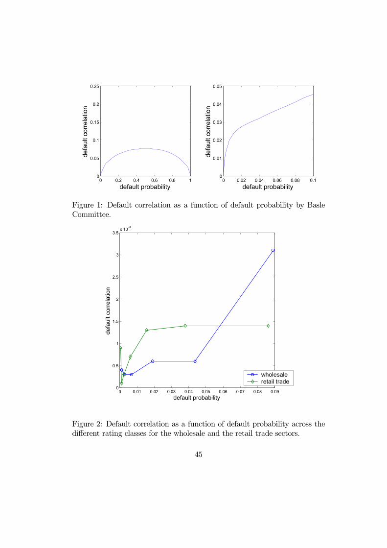
0 0.2 0.4 0.6 0.8 10

0.05

0.1

0.15

0.2

0.25

default probability

defa

ult c

orre

latio

n

0 0.02 0.04 0.06 0.08 0.10

0.01

0.02

0.03

0.04

0.05

default probability

defa

ult c

orre

latio

nFigure 1: Default correlation as a function of default probability by BasleCommittee.

0 0.01 0.02 0.03 0.04 0.05 0.06 0.07 0.08 0.090

0.5

1

1.5

2

2.5

3

3.5x 10-3

default probability

defa

ult c

orre

latio

n

wholesaleretail trade

Figure 2: Default correlation as a function of default probability across thedifferent rating classes for the wholesale and the retail trade sectors.

45

1992 1994 1996 1998 20000.1

0.15

0.2

0.25

0.3class 7

1992 1994 1996 1998 20000.1

0.15

0.2

0.25class 6

1992 1994 1996 1998 20000.1

0.15

0.2

0.25

0.3class 5

1992 1994 1996 1998 20000.1

0.12

0.14

0.16

0.18

0.2

class 3

1992 1994 1996 1998 2000

0.15

0.2

0.25

0.3class 2

1992 1994 1996 1998 20000.05

0.1

0.15class 1

Figure 3: Probabilities of a downgrade of at most 2 buckets for the differentrating classes. The circles (resp. the diamonds) correspond to the wholesale(retail trade) sector.

46

1992 1994 1996 1998 20000.05

0.1

0.15

class 6

1992 1994 1996 1998 20000.2

0.25

0.3

0.35class 5

1992 1994 1996 1998 2000

0.3

0.35

0.4

0.45

0.5

0.55class 4

1992 1994 1996 1998 20000.3

0.35

0.4

class 3

1992 1994 1996 1998 2000

0.4

0.45

0.5

0.55class 2

1992 1994 1996 1998 20000.35

0.4

0.45

0.5class 1

Figure 4: Probabilities of an upgrade of at most 2 buckets for the differentrating classes. The circles (resp. the diamonds) correspond to the wholesale(retail trade) sector.

47

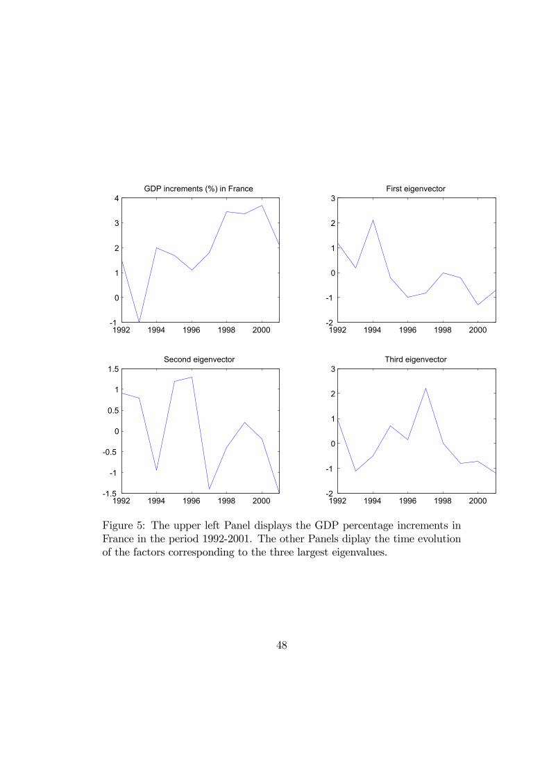
1992 1994 1996 1998 2000-1

0

1

2

3

4GDP increments (%) in France

1992 1994 1996 1998 2000-2

-1

0

1

2

3First eigenvector

1992 1994 1996 1998 2000-1.5

-1

-0.5

0

0.5

1

1.5Second eigenvector

1992 1994 1996 1998 2000-2

-1

0

1

2

3Third eigenvector

Figure 5: The upper left Panel displays the GDP percentage increments inFrance in the period 1992-2001. The other Panels diplay the time evolutionof the factors corresponding to the three largest eigenvalues.

48

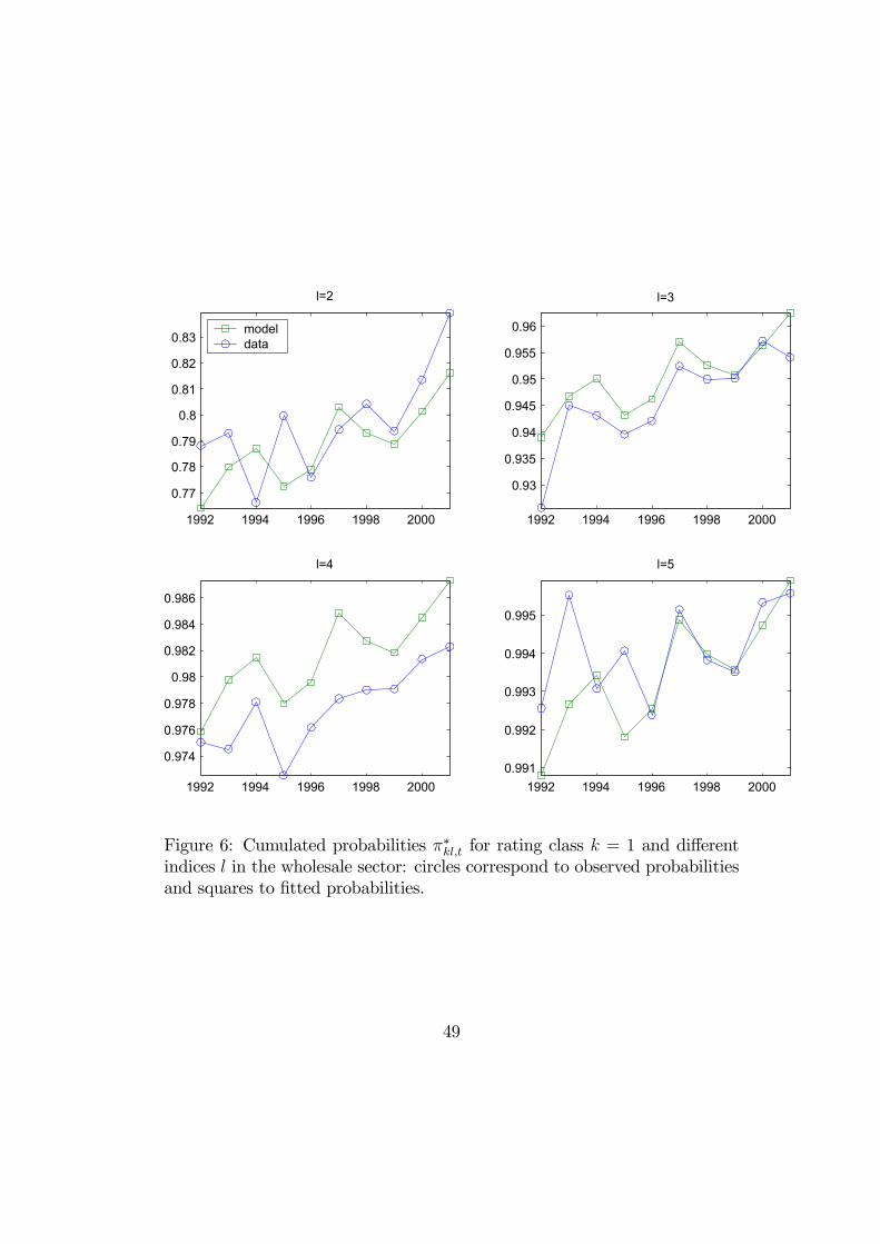
1992 1994 1996 1998 2000

0.77

0.78

0.79

0.8

0.81

0.82

0.83

l=2

1992 1994 1996 1998 2000

0.93

0.935

0.94

0.945

0.95

0.955

0.96

l=3

1992 1994 1996 1998 2000

0.974

0.976

0.978

0.98

0.982

0.984

0.986

l=4

1992 1994 1996 1998 20000.991

0.992

0.993

0.994

0.995

l=5

modeldata

Figure 6: Cumulated probabilities π∗kl,t for rating class k = 1 and differentindices l in the wholesale sector: circles correspond to observed probabilitiesand squares to fitted probabilities.

49

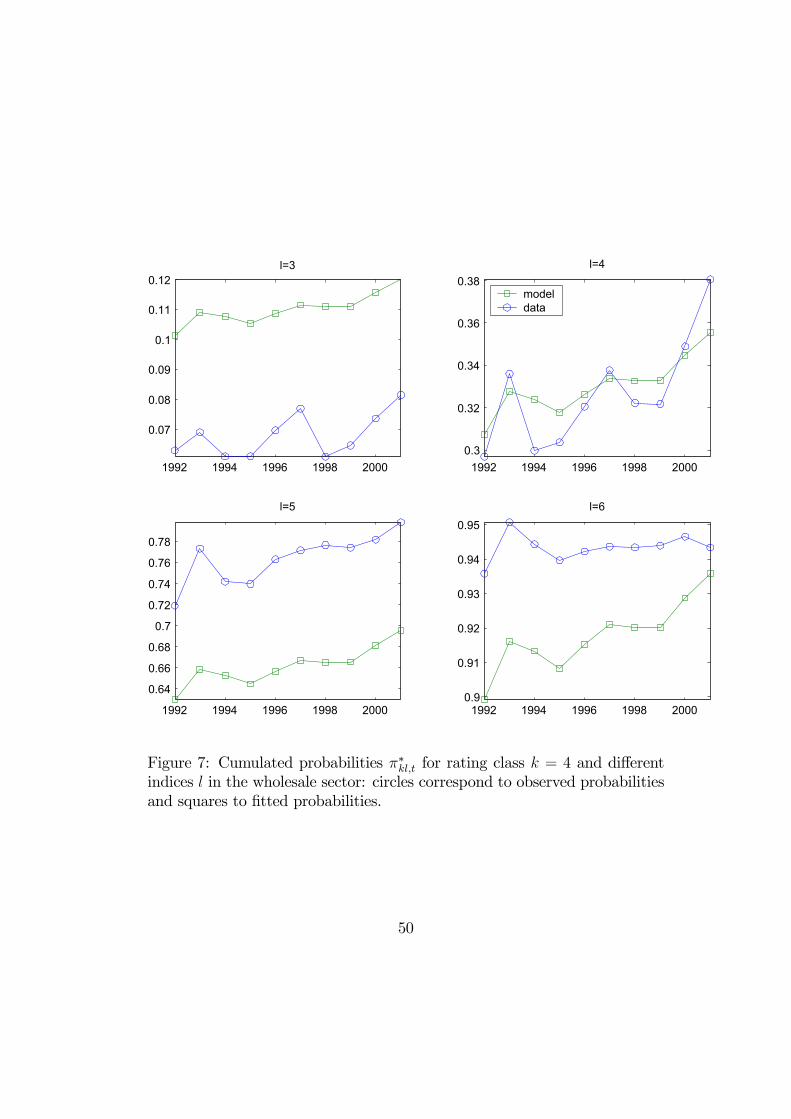
1992 1994 1996 1998 2000

0.07

0.08

0.09

0.1

0.11

0.12l=3

1992 1994 1996 1998 20000.3

0.32

0.34

0.36

0.38l=4

1992 1994 1996 1998 2000

0.64

0.66

0.68

0.7

0.72

0.74

0.76

0.78

l=5

1992 1994 1996 1998 20000.9

0.91

0.92

0.93

0.94

0.95l=6

modeldata

Figure 7: Cumulated probabilities π∗kl,t for rating class k = 4 and differentindices l in the wholesale sector: circles correspond to observed probabilitiesand squares to fitted probabilities.

50