Stochastic Evolutionary Game Dynamics - … · Stochastic Evolutionary Game Dynamics Chris Wallace...
51
Stochastic Evolutionary Game Dynamics Chris Wallace Department of Economics, University of Leicester [email protected] H. Peyton Young Department of Economics, University of Oxford [email protected] Handbook Chapter: Printed November 19, 2013. 1. Evolutionary Dynamics and Equilibrium Selection Game theory is often described as the study of interactive decision-making by rational agents. 1 However, there are numerous applications of game theory where the agents are not fully rational, yet many of the conclusions remain valid. A case in point is biological competition between species, a topic pioneered by Maynard Smith and Price (1973). In this setting the ‘agents’ are representatives of different species that interact and receive payoffs based on their strategic behaviour, whose strategies are hard-wired rather than consciously chosen. The situation is a game because a given strategy’s success depends upon the strate- gies of others. The dynamics are not driven by rational decision-making but by mutation and selection: successful strategies increase in frequency compared to relatively unsuccessful ones. An equilibrium is simply a rest point of the selection dynamics. Under a variety of plausible assumptions about the dynamics, it turns out that these rest points are closely related (though not necessarily identical) to the usual notion of Nash equilibrium in normal form games (Weibull, 1995; Nachbar, 1990; Ritzberger and Weibull, 1995; Sandholm, 2010, particularly Ch. 5). Indeed, this evolutionary approach to equilibrium was anticipated by Nash himself in a key passage of his doctoral dissertation. “We shall now take up the ‘mass-action’ interpretation of equilibrium points. . . [I]t is unnecessary to assume that the participants have full knowledge of the total structure of the game, or the ability and inclination to go through any complex reasoning processes. But the participants are supposed to accumulate empirical information on the relative advantages of the various pure strategies at their disposal. To be more detailed, we assume that there is a population (in the sense of statistics) of participants for each position of the game. Let us also assume that 1 For example, Aumann (1985) puts it thus: “game [. . . ] theory [is] concerned with the interactive behaviour of Homo rationalis —rational man”.
Transcript of Stochastic Evolutionary Game Dynamics - … · Stochastic Evolutionary Game Dynamics Chris Wallace...

Stochastic Evolutionary Game Dynamics
Chris Wallace
Department of Economics, University of Leicester
H. Peyton Young
Department of Economics, University of Oxford
Handbook Chapter: Printed November 19, 2013.
1. Evolutionary Dynamics and Equilibrium Selection
Game theory is often described as the study of interactive decision-making by rational
agents.1 However, there are numerous applications of game theory where the agents are
not fully rational, yet many of the conclusions remain valid. A case in point is biological
competition between species, a topic pioneered by Maynard Smith and Price (1973). In this
setting the ‘agents’ are representatives of different species that interact and receive payoffs
based on their strategic behaviour, whose strategies are hard-wired rather than consciously
chosen. The situation is a game because a given strategy’s success depends upon the strate-
gies of others. The dynamics are not driven by rational decision-making but by mutation
and selection: successful strategies increase in frequency compared to relatively unsuccessful
ones. An equilibrium is simply a rest point of the selection dynamics. Under a variety of
plausible assumptions about the dynamics, it turns out that these rest points are closely
related (though not necessarily identical) to the usual notion of Nash equilibrium in normal
form games (Weibull, 1995; Nachbar, 1990; Ritzberger and Weibull, 1995; Sandholm, 2010,
particularly Ch. 5).
Indeed, this evolutionary approach to equilibrium was anticipated by Nash himself in a key
passage of his doctoral dissertation.
“We shall now take up the ‘mass-action’ interpretation of equilibrium points. . .
[I]t is unnecessary to assume that the participants have full knowledge of the
total structure of the game, or the ability and inclination to go through any
complex reasoning processes. But the participants are supposed to accumulate
empirical information on the relative advantages of the various pure strategies
at their disposal.
To be more detailed, we assume that there is a population (in the sense of
statistics) of participants for each position of the game. Let us also assume that
1For example, Aumann (1985) puts it thus: “game [. . . ] theory [is] concerned with the interactive behaviourof Homo rationalis—rational man”.
2
the ‘average playing’ of the game involves n participants selected at random
from the n populations, and that there is a stable average frequency with which
each pure strategy is employed by the ‘average member’ of the appropriate
population. . . Thus the assumptions we made in this ‘mass-action’ interpreta-
tion lead to the conclusion that the mixed strategies representing the average
behaviour in each of the populations form an equilibrium point. . . .Actually,
of course, we can only expect some sort of approximate equilibrium, since the
information, its utilization, and the stability of the average frequencies will be
imperfect.” (Nash, 1950b, pp. 21–23.)
The key point is that equilibrium does not require the assumption of individual rationality;
it can arise as the average behaviour of a population of players who are less than rational
and operate with ‘imperfect’ information.
This way of understanding equilibrium is in some respects less problematic than the treat-
ment of equilibrium as the outcome of a purely rational, deductive process. One difficulty
with the latter is that it does not provide a satisfactory answer to the question of which
equilibrium will be played in games with multiple equilibria. This is true in even the sim-
plest situations, such as 2×2 coordination games. A second difficulty is that pure rationality
does not provide a coherent account of what happens when the system is out of equilibrium,
that is, when the players’ expectations and strategies are not fully consistent. The biological
approach avoids this difficulty by first specifying how adjustment occurs at the individual
level and then studying the resulting aggregate dynamics. This framework also lends itself
to the incorporation of stochastic effects that may arise from a variety of factors, including
variability in payoffs, environmental shocks, spontaneous mutations in strategies, and other
probabilistic phenomena. The inclusion of persistent stochastic perturbations leads to a dy-
namical theory that helps resolve the question of which equilibria will be selected, because
it turns out that persistent random perturbations can actually make the long-run behaviour
of the process more predictable.
1.1. Evolutionarily Stable Strategies. In an article in Nature in 1973, the biologists
John Maynard Smith and George R. Price introduced the notion of an evolutionarily stable
strategy (or ESS).2 This concept went on to have a great impact in the field of biology; but
the importance of their contribution was also quickly recognized by game theorists working
in economics and elsewhere.
Imagine a large population of agents playing a game. Roughly put, an ESS is a strategy σ
such that, if most members of the population adopt it, a small number of “mutant” players
choosing another strategy σ′ would receive a lower payoff than the vast majority playing σ.
2Maynard Smith and Price (1973). For an excellent exposition of the concept, and details of some of theapplications in biology, see the beautiful short book by Maynard Smith (1982).

3
Rather more formally, consider a 2-player symmetric strategic-form game G. Let S denote
a finite set of pure-strategies for each player (with typical member s), and form the set of
mixed strategies over S, written Σ. Let u(σ, σ′) denote the payoff a player receives from
playing σ ∈ Σ against an opponent playing σ′. Then an ESS is a strategy σ such that
u(σ, εσ′ + (1− ε)σ) > u(σ′, εσ′ + (1− ε)σ), (1)
for all σ′ 6= σ, and for ε > 0 sufficiently small. The idea is this: suppose that there is
a continuum population of individuals each playing σ. Now suppose a small proportion ε
of these individuals “mutate” and play a different strategy σ′. Evolutionary pressure acts
against these mutants if the existing population receives a higher payoff in the post-mutation
world than the mutants themselves do, and vice versa. If members of the population are
uniformly and randomly matched to play G then it is as if the opponent’s mixed strategy
in the post-mutation world is εσ′ + (1 − ε)σ ∈ Σ. Thus, a strategy might be expected to
survive the mutation if (1) holds. If it survives all possible such mutations (given a small
enough proportion of mutants) it is an ESS.
Definition 1a. σ ∈ Σ is an Evolutionarily Stable Strategy (ESS) if for all σ′ 6= σ there
exists some ε(σ′) ∈ (0, 1) such that (1) holds for all ε < ε(σ′).3
An alternative definition is available that draws out the connection between an ESS and a
Nash equilibrium strategy. Note that an ESS must be optimal against itself. If this were not
the case there necessarily would be a better response to σ than σ itself and, by continuity
of u, a better response to an ε mix of this strategy with σ than σ itself (for small enough ε).
Therefore an ESS must be a Nash equilibrium strategy.
But an ESS requires more than the Nash property. In particular, consider an alternative
best reply σ′ to a candidate ESS σ. If σ is not also a better reply to σ′ than σ′ is to itself
then σ′ must earn at least what σ earns against any mixture of the two. But then this is
true for an ε mix and hence σ cannot be an ESS. This suggests the following definition.
Definition 1b. σ is an ESS if and only if (i) it is a Nash equilibrium strategy, u(σ, σ) ≥u(σ′, σ) for all σ′; and (ii) if u(σ, σ) = u(σ′, σ) then u(σ, σ′) > u(σ′, σ′) for all σ′ 6= σ.
Definitions 1a and 1b are equivalent. The latter makes it very clear that the set of ESS is a
subset of the set of Nash equilibrium strategies. Note moreover that if a Nash equilibrium
is strict, then its strategy must be evolutionarily stable.
One important consequence of the strengthening of the Nash requirement is that there are
games for which no ESS exists. Consider, for example, a non-zero sum version of the ‘Rock-
Scissors-Paper’ game in which pure strategy 3 beats strategy 2, which in turn beats strategy
1, which in turn beats strategy 3. Suppose payoffs are 4 for a winning strategy, 1 for a losing
3This definition was first presented by Taylor and Jonker (1978). The original definition (Maynard Smithand Price, 1973; Maynard Smith, 1974) is given below.

4
strategy, and 3 otherwise. The unique (symmetric) Nash equilibrium strategy is σ = (13, 1
3, 1
3),
but this is not an ESS. For instance, a mutant playing Rock (strategy 1) will get a payoff of83
against σ, which is equal to the payoff received by an individual playing σ against σ. As
a consequence, the second condition of Definition 1b must be checked. However, playing σ
against Rock generates a payoff of 83< 3, which is less than what the mutant would receive
from playing against itself: there is no ESS.4
There is much more that could be said about this and other static evolutionary concepts,
but the focus here is on stochastic dynamics. Weibull (1995) and Sandholm (2010) provide
excellent textbook treatments of the deterministic dynamics approach to evolutionary games;
see also Sandholm’s chapter in this volume.
1.2. Stochastically Stable Sets. An ESS suffers from two important limitations. First,
it is guaranteed only that such strategies are stable against single-strategy mutations; the
possibility that multiple mutations may arise simultaneously is not taken into account (and,
indeed, an ESS is not necessarily immune to these kinds of mutations). The second limita-
tion is that ESS treats mutations as if they were isolated events, and the system has time to
return to its previous state before the next mutation occurs. In reality however there is no
reason to think this is the case: populations are continually being subjected to small per-
turbations that arise from mutation and other chance events. A series of such perturbations
in close succession can kick the process out of the immediate locus of an ESS; how soon it
returns depends on the global structure of the dynamics, not just on its behaviour in the
neighbourhood of a given ESS. These considerations lead to a selection concept known as
stochastic stability that was first introduced by Foster and Young (1990). The remainder of
this section follows the formulation in that paper. In the next section we shall discuss the
discrete-time variants introduced by Kandori, Mailath, and Rob (1993) and Young (1993a).
As a starting point, consider the replicator dynamics of Taylor and Jonker (1978). These
dynamics are not stochastic—but are meant to capture the underlying stochastic nature
of evolution. Consider a continuum of individuals playing the game G over (continuous)
time. Let ps(t) be the proportion of the population playing pure strategy s at time t. Let
p(t) = [ps(t)]s∈S be the vector of proportions playing each of the strategies in S: this is the
state of the system at t. The simplex Σ ={p(t) :
∑s∈S ps(t) = 1
}describes the state space.
The replicator dynamics capture the idea that a particular strategy will grow in popularity
(the proportion of the population playing it will increase) whenever it is more successful
than average against the current population state. Since G is symmetric, its payoffs can
be collected in a matrix A where ass′ is the payoff a player would receive when playing s
against strategy s′. If a proportion of the population ps′(t) is playing s′ at time t then, given
4The argument also works for the standard zero-sum version of the game: here, when playing against itself,the mutant playing Rock receives a payoff exactly equal to that an individual receives when playing σ againstRock—the second condition of Definition 1b fails again. The “bad” Rock-Scissors-Paper game analyzed inthe above reappears in the example of Figure 9, albeit to illustrate a different point.

5
any individual is equally likely to meet any other, the payoff from playing s at time t is∑s′∈S ass′ps′(t), or the sth element of the vector Ap(t), written [Ap(t)]s. The average payoff
in the population at t is then given by p(t)TAp(t). The replicator dynamics may be written
ps(t)/ps(t) = [Ap(t)]s − p(t)TAp(t), (2)
the proportion playing strategy s increases at a rate equal to the difference between its payoff
in the current population and the average payoff received in the current population.
Although these dynamics are deterministic they are meant to capture the underlying sto-
chastic nature of evolution. They do so only as an approximation. One key difficulty is that
typically there will be many rest-points of these dynamics. They are history dependent: the
starting point in the state space will determine the evolution of the system. Moreover, once
ps is zero, it remains zero forever: the boundaries of the simplex state space are absorbing.
Many of these difficulties can be overcome with an explicit treatment of stochastic evolution-
ary pressures. This led Foster and Young (1990) to consider a model directly incorporating
a stochastic element into evolution and to introduce the idea of stochastically stable sets
(SSS).5
Suppose there is a stochastic dynamical system governing the evolution of strategy play and
indexed by a level of noise ε (e.g. the probability of mutation). Roughly speaking, a state
p is stochastically stable if, in the long run, it is nearly certain that the system lies within
a small neighbourhood of p as ε → 0. To be more concrete, consider a model of evolution
where the noise is well approximated by the following Wiener process
dps(t) = ps(t){
[Ap(t)]s − p(t)TAp(t)}dt+ ε[Γ(p)dW (t)]s. (3)
We assume that: (i) Γ(p) is continuous in p and strictly positive for p 6= 0; (ii) pTΓ(p) = 0T ;
and (iii)W (t) is a continuous white noise process with zero mean and unit variance-covariance
matrix. In order to avoid complications arising from boundary behaviour, we shall suppose
that each pi is bounded away from zero (say owing to a steady inflow of migrants).6 Thus
we shall study the behaviour of the process in an interior envelope of the form
S∆ = {p ∈ S : pi ≥ ∆ > 0 for all i} . (4)
We remark that the noise term can capture a wide variety of stochastic perturbations in ad-
dition to mutations. For example, the payoffs in the game may vary between encounters, the
number of encounters may vary in a given time period. Aggregated over a large population,
these variations will be very nearly normally distributed.
The replicator dynamic in (3) is constantly affected by noise indexed by ε; the interior of the
state space is appropriate since mutation would keep the process away from the boundary
so avoiding absorption when a strategy dies out (ps(t) = 0). The idea is to find which
5They use dynamical systems methods which build upon those found in Freidlin and Wentzell (1998).6The boundary behaviour of the process is discussed in detail in Foster and Young (1990, 1997). See alsoFudenberg and Harris (1992).

6
state(s) the process spends most time close to when the noise is driven from the system
(ε→ 0). For any given ε, calculate the limiting distribution of p(t) as t→∞. Now, letting
ε→ 0, if a particular population state p∗ has strictly positive weight in every neighbourhood
surrounding it in the resulting limiting distribution then it is said to be stochastically stable.
The stochastically stable set is simply the collection of such states.
Definition 2. The state p∗ is stochastically stable if, for all δ > 0,
lim supε→0
∫Nδ(p∗)
fε(p)dp > 0,
where Nδ(p∗) = {p : |p− p∗| < δ}, and fε(p) is the limiting density of p(t) as t→∞, which
exists because of our assumptions on Γ(p). The stochastically stable set (SSS) is the minimal
set of p∗ for which this is true.
In words, “a stochastically stable set (SSS) is the minimal set of states S such that, in the
long run, it is nearly certain that the process lies within every open set containing S as the
noise tends slowly to zero” (Foster and Young, 1990, p. 221). As it turns out the SSS is
often a single state, say p∗. In this case the process is contained within an arbitrarily small
neighbourhood of p∗ with near certainty when the noise becomes arbitrarily small.
Consider the symmetric 2× 2 pure coordination game A:
A =
[1 0
0 2
]This game has two ESS, in which everyone is playing the same strategy (either 1 or 2). It
also has a mixed Nash equilibrium (23, 1
3) that is not an ESS. Let us examine the behaviour of
the dynamics when a small stochastic term is introduced. Let p(t) be the proportion playing
strategy 1 at time t. Assume for simplicity that the stochastic disturbance is uniform in
space and time. We then obtain a stochastic differential equation of form
dp(t) = p(t)[p(t)− p2(t)− 2(1− p(t))2]dt+ εdW (t), (5)
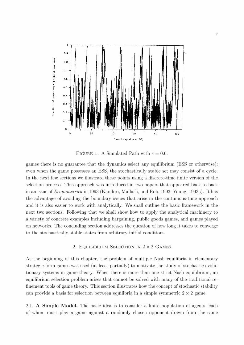
where W (t) is N(0, t). Figure 1 shows a simulated path with ε = 0.6 and initial condition
p(0) = 0.5. Notice that, on average, the process spends more time near the all-2 state than it
does near the all-1 states, but it does not converge to the all-2 state. In this simulation the
noise level, ε is actually quite large. This illustrates the general point that the noise level
does not need to be taken to zero for a significant selection bias toward the stochastically
stable state (in this case all-2) to be revealed. When ε = 0.2, for example, the process is
very close to all-2 with very high probability in the long run.
In general, there is no guarantee that the stochastically stable equilibrium of a 2× 2 coordi-
nation game is Pareto dominant. Indeed, under fairly general conditions the dynamics favour
the risk-dominant equilibrium, as we shall see in the next section. Furthermore, in larger
7
Figure 1. A Simulated Path with ε = 0.6.
games there is no guarantee that the dynamics select any equilibrium (ESS or otherwise):
even when the game possesses an ESS, the stochastically stable set may consist of a cycle.
In the next few sections we illustrate these points using a discrete-time finite version of the
selection process. This approach was introduced in two papers that appeared back-to-back
in an issue of Econometrica in 1993 (Kandori, Mailath, and Rob, 1993; Young, 1993a). It has
the advantage of avoiding the boundary issues that arise in the continuous-time approach
and it is also easier to work with analytically. We shall outline the basic framework in the
next two sections. Following that we shall show how to apply the analytical machinery to
a variety of concrete examples including bargaining, public goods games, and games played
on networks. The concluding section addresses the question of how long it takes to converge
to the stochastically stable states from arbitrary initial conditions.
2. Equilibrium Selection in 2× 2 Games
At the beginning of this chapter, the problem of multiple Nash equilibria in elementary
strategic-form games was used (at least partially) to motivate the study of stochastic evolu-
tionary systems in game theory. When there is more than one strict Nash equilibrium, an
equilibrium selection problem arises that cannot be solved with many of the traditional re-
finement tools of game theory. This section illustrates how the concept of stochastic stability
can provide a basis for selection between equilibria in a simple symmetric 2× 2 game.
2.1. A Simple Model. The basic idea is to consider a finite population of agents, each
of whom must play a game against a randomly chosen opponent drawn from the same

8
population. They do so in (discrete) time. Each period some of the players may revise their
strategy choice. Since revision takes place with some noise (it is a stochastic process), after
sufficient time any configuration of strategy choices may be reached by the process from any
other.
To illustrate these ideas, consider a simple symmetric coordination game in which two players
have two strategies each. Suppose the players must choose between X and Y and that payoffs
are as given in the following game matrix:
X Y
Xa
ac
b
Yb
cd
d
Figure 2. A 2× 2 Coordination Game.
Suppose that a > c and d > b, so that the game has two pure Nash equilibria, (X,X) and
(Y,Y). It will also have a (symmetric) mixed equilibrium, and elementary calculations show
that this equilibrium requires the players to place probability p on pure action X, where
p =(d− b)
(a− c) + (d− b)∈ (0, 1).
Now suppose there is a finite population of n agents. At each period t ∈ {0, . . . ,∞} one
of the agents is selected to update their strategy. Suppose that agent i is chosen from the
population with probability 1n
for all i.7 In a given period t, an updating agent plays a
best reply to the mixed strategy implied by the configuration of other agents’ choices in
period t − 1 with high probability. With some low probability, however, the agent plays
the strategy that is not a best reply.8 The state at time t may be characterized by a single
number, xt ∈ {0, . . . , n}: the number of agents at time t who are playing strategy X. The
number of agents playing Y is then simply yt = n− xt.
Suppose an agent i who in period t− 1 was playing Y is chosen to update in period t. Then
xt−1 other agents were playing X and n−xt−1−1 other agents were playing Y. The expected
payoff for player i from X is larger only if
xt−1
n− 1a+
n− xt−1 − 1
n− 1b >
xt−1
n− 1c+
n− xt−1 − 1
n− 1d ⇔ xt−1
n− 1> p.
In this case, player i is then assumed to play the best reply X with probability 1−ε, and the
non-best reply Y with probability ε. Similarly, a player j who played X in period t−1 plays
X with probability 1−ε and Y with probability ε if (xt−1−1)/(n−1) > p. It is then possible
7The argument would not change at all so long as each agent is chosen with some strictly positive probabilityρi > 0. For notational simplicity the uniform case is assumed here.8This process would make sense if, for example, the agent was to play the game n − 1 times against eachother agent in the population at time t, or against just one of the other agents drawn at random. The lowprobability “mutation” might then be interpreted as a mistake on the part of the revising agent.
9
to calculate the transition probabilities between the various states for this well-defined finite
Markov chain, and examine the properties of its ergodic distribution.
2.2. The Unperturbed Process. Consider first the process when ε = 0 (an “unperturbed”
process). Suppose a single agent is selected to revise in each t. In this case, if selected to
revise, the agent will play a best reply to the configuration of opponents’ choices in the
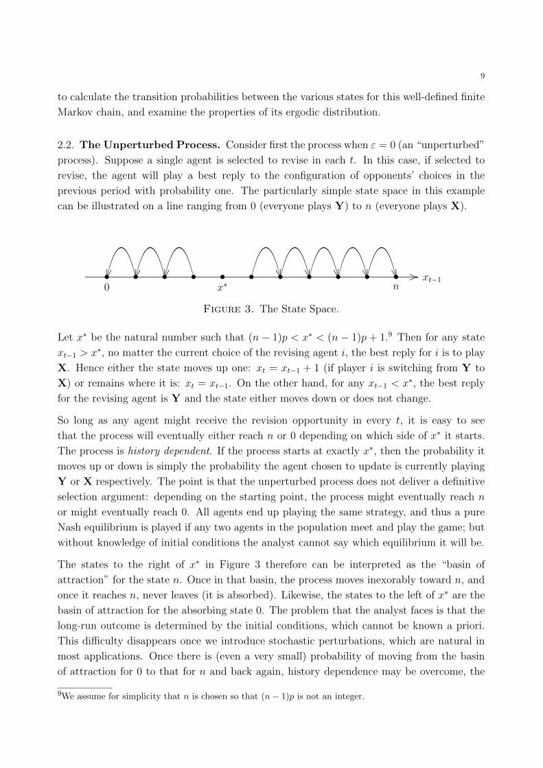
previous period with probability one. The particularly simple state space in this example
can be illustrated on a line ranging from 0 (everyone plays Y) to n (everyone plays X).
..............................................................................................................................................................................................................................................................................................................................................................................................................................................................................................................................................................................................................................................................................................................................................................................................................................................................................................................
.......
.......
.......
.
.......................
.......
.......
.......
.
.......................
.......
.......
.......
.
.......
.......
.......
.
.......................
.......
.......
.......
.
.......................
.......
.......
.......
.
.......................
.......
.......
.......
.
.......................
.......
.......
.......
.
.......................
..................................................................................................................................................................................................
..............................................................................................................................................................................................
.......................................................................................................................................................................................... ....
..............................................................................................................................................................................................
..............................................................................................................................................................................................
..............................................................................................................................................................................................
..............................................................................................................................................................................................
..............................................................................................................................................................................................................................................................................
........................• • • • • • • • • • •
0 nx∗xt−1
Figure 3. The State Space.
Let x∗ be the natural number such that (n− 1)p < x∗ < (n− 1)p + 1.9 Then for any state
xt−1 > x∗, no matter the current choice of the revising agent i, the best reply for i is to play
X. Hence either the state moves up one: xt = xt−1 + 1 (if player i is switching from Y to
X) or remains where it is: xt = xt−1. On the other hand, for any xt−1 < x∗, the best reply
for the revising agent is Y and the state either moves down or does not change.
So long as any agent might receive the revision opportunity in every t, it is easy to see
that the process will eventually either reach n or 0 depending on which side of x∗ it starts.
The process is history dependent. If the process starts at exactly x∗, then the probability it
moves up or down is simply the probability the agent chosen to update is currently playing
Y or X respectively. The point is that the unperturbed process does not deliver a definitive
selection argument: depending on the starting point, the process might eventually reach n
or might eventually reach 0. All agents end up playing the same strategy, and thus a pure
Nash equilibrium is played if any two agents in the population meet and play the game; but
without knowledge of initial conditions the analyst cannot say which equilibrium it will be.
The states to the right of x∗ in Figure 3 therefore can be interpreted as the “basin of
attraction” for the state n. Once in that basin, the process moves inexorably toward n, and
once it reaches n, never leaves (it is absorbed). Likewise, the states to the left of x∗ are the
basin of attraction for the absorbing state 0. The problem that the analyst faces is that the
long-run outcome is determined by the initial conditions, which cannot be known a priori.
This difficulty disappears once we introduce stochastic perturbations, which are natural in
most applications. Once there is (even a very small) probability of moving from the basin
of attraction for 0 to that for n and back again, history dependence may be overcome, the
9We assume for simplicity that n is chosen so that (n− 1)p is not an integer.
10
Markov process becomes irreducible, and a unique (ergodic) distribution will characterize
long-run play.
Recall the objective is to identify the stochastically stable states of such a process. This
is equivalent to asking which state(s) are played almost all of the time as the stochastic
perturbations introduced to the system are slowly reduced in size. For such vanishingly
small perturbations (in this model, ε → 0) the process will spend almost all time local to
one of the equilibrium states 0 or n: this state is stochastically stable and the equilibrium
it represents (in the sense that at 0 all players are playing Y, and at n all the players are
playing X) is said to have been “selected”.
2.3. The Perturbed Process. Consider now the Markov process described above for small
but positive ε > 0. The transition probabilities for an updating agent may be calculated
directly:10
Pr[xt = xt−1 + 1 |xt−1 > x∗] = (1− ε)n− xt−1
n,
Pr[xt = xt−1 |xt−1 > x∗] = (1− ε)xt−1
n+ ε
n− xt−1
n, (6)
Pr[xt = xt−1 − 1 |xt−1 > x∗] = εxt−1
n.
The first probability derives from the fact that the only way to move up a state is if first
a Y-playing agent is selected to revise, and second the agent chooses X (a best reply when
xt−1 > x∗) which happens with high probability (1 − ε). The second transition requires
either an X-playing revising agent to play a best reply, or a Y-playing reviser to err. The
final transition in (6) requires an X-player to err. Clearly, conditional on the state being
above x∗, all other transition probabilities are zero.
An analogous set of transition probabilities may be written down for xt−1 < x∗ using exactly
the logic presented in the previous paragraph. For xt−1 = x∗, the process moves down only
if an X-player is selected to revise and with high probability selects the best reply Y. The
process moves up only if a Y-player is selected to revise and with high probability selects
the best reply X. The process stays at x∗ with low probability, only if whichever agent is
selected fails to play a best reply (so this transition probability is simply ε).
As a result, it is easy to see that any state may be reached from any other with positive
probability, and every state may transit to itself. These two facts together guarantee that
the Markov chain is irreducible and aperiodic, and therefore that there is a unique “ergodic”
long-run distribution governing the frequency of play. The π = (π0, . . . , πn) that satisfies
π = Pπ where P = [pi→j] is the matrix of transition probabilities is the ergodic distribution.
10For the sake of exposition it is assumed that agents are selected to update uniformly, so that the probabilitythat agent i is revising at time t is 1
n . The precise distribution determining the updating agent is largelyirrelevant, so long as it places strictly positive probability on each agent i.

11
Note that P takes a particularly simple form: the probability of transiting from state i
to state j is pi→j = 0 unless i = j or i = j ± 1 (so P is tridiagonal). It is algebraically
straightforward to confirm that for such a process pi→jπi = pj→iπj for all i, j.
Combining these equalities for values of i and j such that pi→j > 0, along with the fact that∑i πi = 1, one obtains a (unique) solution for π. Indeed, consider the expression,
πnπ0
=
(p0→1
p1→0
)× . . .×
(p(n−1)→n
pn→(n−1)
), (7)
which follows from an immediate algebraic manipulation of pi→jπi = pj→iπj. The (positive)
transition probabilities in (7) are given by the expressions in (6). Consider a transition to
the left of x∗: the probabilities of moving from state i to state i+1 and of moving from state
i+ 1 to state i are
pi→i+1 = εn− in
and pi+1→i = (1− ε)i+ 1
n.
To the right of x∗, these probabilities are
pi→i+1 = (1− ε)n− in
and pi+1→i = εi+ 1
n.
Combining these probabilities and inserting into the expression in (7) yields
πnπ0
=x∗−1∏i=0
(ε
1− ε
)(n− ii+ 1
)×
n−1∏i=x∗
(1− εε
)(n− ii+ 1
)
=
(ε
1− ε
)x∗ (1− εε
)n−x∗= ε2x∗−n(1− ε)n−2x∗ . (8)
It is possible to write down explicit solutions for πi for all i ∈ {0, . . . , n} as a function
of ε. However, the main interest lies in the ergodic distribution for ε → 0. When the
perturbations die away, the process becomes stuck for longer and longer close to one of the
two equilibrium states. Which one? The relative weight in the ergodic distribution placed
on the two equilibrium states is πn/π0. Thus, we are interested in the limit:
limε→0
πnπ0
= limε→0
ε2x∗−n(1− ε)n−2x∗ = limε→0
ε2x∗−n =
{0 if x∗ > n
2,
∞ if x∗ < n2.
It is straightforward to show that the weight in the ergodic distribution placed on all other
states tends to zero as ε → 0. Thus if x∗ > n2, πn → 0 and π0 → 1: all weight congregates
at 0. Every agent in the population is playing Y almost all of the time: the equilibrium
(Y,Y) is selected. Now, recall that (n − 1)p < x∗ < (n − 1)p + 1. For n sufficiently large,
the inequality x∗ > n2
is well approximated by p > 12. (Y,Y) is selected if p > 1
2; that is if
c+ d > a+ b. If the reverse strict inequality holds then (X,X) is selected.
Looking back at the game in Figure 2, note that this is precisely the condition in a symmetric
2×2 game for the equilibrium to be risk-dominant (Harsanyi and Selten, 1988). A stochastic
evolutionary dynamic of the sort introduced here selects the risk-dominant Nash equilibrium
12
in a 2 × 2 symmetric game. This remarkable selection result appears in both Kandori,
Mailath, and Rob (1993) and Young (1993a), who nevertheless arrive at the result from
quite different adjustment processes.
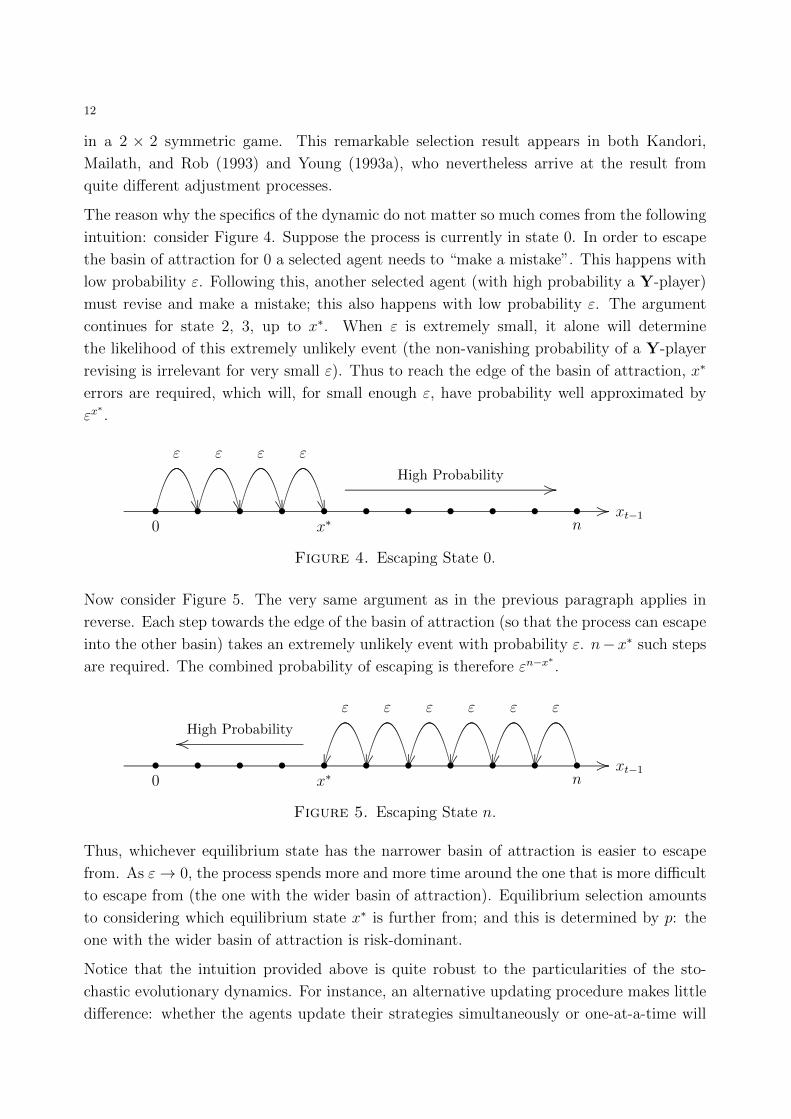
The reason why the specifics of the dynamic do not matter so much comes from the following
intuition: consider Figure 4. Suppose the process is currently in state 0. In order to escape
the basin of attraction for 0 a selected agent needs to “make a mistake”. This happens with
low probability ε. Following this, another selected agent (with high probability a Y-player)
must revise and make a mistake; this also happens with low probability ε. The argument
continues for state 2, 3, up to x∗. When ε is extremely small, it alone will determine
the likelihood of this extremely unlikely event (the non-vanishing probability of a Y-player
revising is irrelevant for very small ε). Thus to reach the edge of the basin of attraction, x∗
errors are required, which will, for small enough ε, have probability well approximated by
εx∗.
..............................................................................................................................................................................................................................................................................................................................................................................................................................................................................................................................................................................................................................................................................................................................................................................................................................................................................................................
.......
.......
.......
.
.......................
.......
.......
.......
.
.......................
.......
.......
.......
.
.......................
.......
.......
.......
.
..................................................................................................................................................................................................
..............................................................................................................................................................................................
..............................................................................................................................................................................................
.......................................................................................................................................................................................... ....................................................................................
........................
..........................................................................................................................................................................................................................................................................................................................................................................................................................................................
....High Probability
• • • • • • • • • • •
ε ε ε ε
0 nx∗xt−1
Figure 4. Escaping State 0.
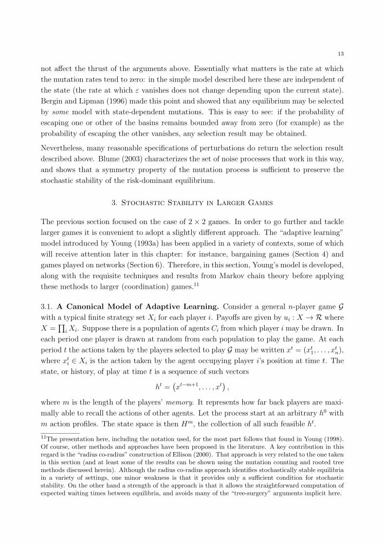
Now consider Figure 5. The very same argument as in the previous paragraph applies in
reverse. Each step towards the edge of the basin of attraction (so that the process can escape
into the other basin) takes an extremely unlikely event with probability ε. n−x∗ such steps
are required. The combined probability of escaping is therefore εn−x∗.
.............................................................................................................................................................................................................................................................................................................................................................................................................................................................................................................................................................................................................................................................................................................................................................................................................................................................................................................
.......................
.......
.......
.......
.
.......................
.......
.......
.......
.
.......................
.......
.......
.......
.
.......................
.......
.......
.......
.
.......................
.......
.......
.......
.
.......................
..................................................................................................................................................................................................
..............................................................................................................................................................................................
..............................................................................................................................................................................................
..............................................................................................................................................................................................
..............................................................................................................................................................................................
..............................................................................................................................................................................................................................................................................
........................
.......................................................................................................................................................................................................................................................................
........................
High Probability
• • • • • • • • • • •
εεεεεε
0 nx∗xt−1
Figure 5. Escaping State n.
Thus, whichever equilibrium state has the narrower basin of attraction is easier to escape
from. As ε→ 0, the process spends more and more time around the one that is more difficult
to escape from (the one with the wider basin of attraction). Equilibrium selection amounts
to considering which equilibrium state x∗ is further from; and this is determined by p: the
one with the wider basin of attraction is risk-dominant.
Notice that the intuition provided above is quite robust to the particularities of the sto-
chastic evolutionary dynamics. For instance, an alternative updating procedure makes little
difference: whether the agents update their strategies simultaneously or one-at-a-time will
13
not affect the thrust of the arguments above. Essentially what matters is the rate at which
the mutation rates tend to zero: in the simple model described here these are independent of
the state (the rate at which ε vanishes does not change depending upon the current state).
Bergin and Lipman (1996) made this point and showed that any equilibrium may be selected
by some model with state-dependent mutations. This is easy to see: if the probability of
escaping one or other of the basins remains bounded away from zero (for example) as the
probability of escaping the other vanishes, any selection result may be obtained.
Nevertheless, many reasonable specifications of perturbations do return the selection result
described above. Blume (2003) characterizes the set of noise processes that work in this way,
and shows that a symmetry property of the mutation process is sufficient to preserve the
stochastic stability of the risk-dominant equilibrium.
3. Stochastic Stability in Larger Games
The previous section focused on the case of 2 × 2 games. In order to go further and tackle
larger games it is convenient to adopt a slightly different approach. The “adaptive learning”
model introduced by Young (1993a) has been applied in a variety of contexts, some of which
will receive attention later in this chapter: for instance, bargaining games (Section 4) and
games played on networks (Section 6). Therefore, in this section, Young’s model is developed,
along with the requisite techniques and results from Markov chain theory before applying
these methods to larger (coordination) games.11
3.1. A Canonical Model of Adaptive Learning. Consider a general n-player game Gwith a typical finite strategy set Xi for each player i. Payoffs are given by ui : X → R where
X =∏
iXi. Suppose there is a population of agents Ci from which player i may be drawn. In
each period one player is drawn at random from each population to play the game. At each
period t the actions taken by the players selected to play G may be written xt = (xt1, . . . , xtn),
where xti ∈ Xi is the action taken by the agent occupying player i’s position at time t. The
state, or history, of play at time t is a sequence of such vectors
ht =(xt−m+1, . . . , xt
),
where m is the length of the players’ memory. It represents how far back players are maxi-
mally able to recall the actions of other agents. Let the process start at an arbitrary h0 with
m action profiles. The state space is then Hm, the collection of all such feasible ht.
11The presentation here, including the notation used, for the most part follows that found in Young (1998).Of course, other methods and approaches have been proposed in the literature. A key contribution in thisregard is the “radius co-radius” construction of Ellison (2000). That approach is very related to the one takenin this section (and at least some of the results can be shown using the mutation counting and rooted treemethods discussed herein). Although the radius co-radius approach identifies stochastically stable equilibriain a variety of settings, one minor weakness is that it provides only a sufficient condition for stochasticstability. On the other hand a strength of the approach is that it allows the straightforward computation ofexpected waiting times between equilibria, and avoids many of the “tree-surgery” arguments implicit here.

14
At any time t+ 1, each of the agents selected to play G observes a sample (without replace-
ment) of the history of the other players’ actions. Suppose the size of the sample observed
is s ≤ m. The sample seen by player i of the actions taken by player j 6= i is drawn inde-
pendently from i’s sample of k 6= j and so forth. Upon receipt of such a sample, each player
plays a best reply to the strategy frequencies present in the sample with high probability;
with low probability an action is chosen uniformly at random. The probability an action is
taken at random is written ε. Together, these rules define a Markov process on Hm.
Definition 3. The Markov process Pm,s,ε on the state space Hm described in the text above
is called adaptive play with memory m, sample size s, and error rate ε.
Consider a history of the form h∗ = (x∗, . . . , x∗) where x∗ is a Nash equilibrium of the game.
If the state is currently h∗ then a player at t+ 1 will certainly receive s copies of the sample
x∗−i of the other players’ actions. Since these were Nash strategies, player i’s best reply is
of course x∗i . Thus, for example, were ε = 0, then ht+1 = h∗. In other words, once the
(deterministic) process Pm,s,0 reaches h∗ it will never leave. For this reason, h∗ is called a
“convention”. Moreover it should be clear that all conventions consist of states of the form
(x∗, . . . , x∗) where x∗ is a Nash equilibrium of G. This fact is summarized in the following
proposition.
Proposition 1. The absorbing states of the process Pm,s,0 are precisely the conventions
h∗ = (x∗, . . . , x∗) ∈ Hm, where x∗ is a (strict) Nash equilibrium of G.
When ε > 0 the process will move away from a convention with some low probability. If there
are multiple Nash equilibria, and hence multiple conventions, the process can transit from
any convention to any other with positive probability. The challenge is to characterize the
stationary distribution (written µm,s,ε) for any such error rate. This distribution is unique for
all ε > 0 because the Markov process implicit in adaptive play is irreducible (it is ergodic).
Thus, in order to find the stochastically stable convention, the limit limε→0 µm,s,ε may be
found. This is the goal of the next subsection.
3.2. Markov Processes and Rooted Trees. Hm is the state space for a finite Markov
chain induced by the adaptive play process Pm,s,ε described in the previous subsection.
Suppose that P ε is the matrix of transition probabilities for this Markov chain, where the
(h, h′)th element of the matrix is the transition probability of moving from state h to state
h′ in exactly one period: ph→h′ . Assume ε > 0.
Note that although many such transition probabilities will be zero, the probability of tran-
siting from any state h to any other h in a finite number of periods is strictly positive. To see
this, consider an arbitrary pair (h, h) such that ph→h = 0. Starting at ht = h, in period t+1,
the first element of h disappears and is replaced with a new element in position m. That is,
if ht = h = (x1, x2, . . . , xm) then ht+1 = (x2, . . . , xm, y) where y is the vector of actions taken
15
at t+ 1. Any vector of actions may be taken with positive probability at t+ 1. Therefore, if
h = (x1, x2, . . . , xm), let y = x1. Furthermore, at t+ 2, any vector of actions may be taken,
and in particular x2 can be taken. In this way the elements of h can be replaced in m steps
with the elements of h. With positive probability h transits to h.
This fact means that the Markov chain is irreducible. An irreducible chain with transition
matrix P has a unique invariant (or stationary) distribution µ such that µP = µ. The vector
of stationary probabilities for the process Pm,s,ε, written µm,s,ε, can in principle be found
by solving this matrix equation. This turns out to be computationally difficult however. A
much more convenient approach is method of rooted trees, which we shall now describe.
Think of each state h as the node of a complete directed graph on Hm, and, in a standard
notation, let |Hm| be the number of states (or nodes) in the set Hm.
Definition 4. A rooted tree at h ∈ Hm is a set T of |Hm| − 1 directed edges on the set of
nodes Hm such that for every h′ 6= h there is a unique directed path in T from h′ to h. Let
Th denote the set of all such rooted trees at state (or node) h.
For example, with just two states h and h′, there is a single rooted tree at h (consisting of
the directed edge from h′ to h) and a single rooted tree at h′ (consisting of the directed edge
from h to h′). With three states, h, h′, h′′, there are three rooted trees at each state. For
example, the directed edges from h′′ to h′ and from h′ to h constitute a rooted tree at h, as
do the edges from h′′ to h and from h′ to h, as do the edges from h′ to h′′ and from h′′ to h.
Thus Th consists of these three elements.
As can be seen from these examples, a directed edge may be written as a pair (h, h′) ∈Hm × Hm to be read “the directed edge from h to h′”. Consider a subset of such pairs
S ⊆ Hm ×Hm. Then, for an irreducible process Pm,s,ε on Hm, write
p(S) =∏
(h,h′)∈S
ph→h′ and η(h) =∑T∈Th
p(T ) for all h ∈ Hm. (9)
p(S) is the product of the transition probabilities from h to h′ along the edges in S. When
S is a rooted tree, these edges correspond to paths along the tree linking every state with
the root h. p(S) is called the likelihood of such a rooted tree S. η(h) is then the sum of all
such likelihoods of the rooted trees at h. These likelihoods may be related to the stationary
distribution of any irreducible Markov process. The following proposition is an application
of a result known as the Markov Chain Tree Theorem.
Proposition 2. Each element µm,s,ε(h) in the stationary distribution µm,s,ε of the Markov
process Pm,s,ε is proportional to the sum of the likelihoods of the rooted trees at h:
µm,s,ε(h) = η(h)/ ∑
h′∈Hm
η(h′). (10)
16
Of interest is the ratio of µm,s,ε(h) to µm,s,ε(h′) for two different states h and h′ as ε → 0.
From the expression in (10), this ratio is precisely η(h)/η(h′). Consider the definitions in
(9). Note that many of the likelihoods p(T ) will be zero: transitions are impossible between
many pairs of states h and h′. In the cases where p(T ) is positive, what matters is the rate
at which the various terms vanish as ε → 0. As the noise is driven from the system, those
p(T ) that vanish quickly will play no role in the summation term on the right-hand side
of the second expression in (9). Only those that vanish slowly will remain: it is the ratio
of these terms that will determine the relative weights of µ∗(h) and µ∗(h′) therefore. This
observation is what drives the results later in this section; and indeed those used throughout
this chapter.
Of course, calculating these likelihoods may be a lengthy process: the number of rooted
trees at each state can be very large (particularly if s is big, or the game itself has many
strategies). Fortunately, there is a shortcut that allows the stationary distribution of the
limiting process (as ε → 0) to be characterized using a smaller (related) graph, where each
node corresponds to a different pure Nash equilibrium of G.12 Again, an inspection of (9)
and (10) provides the intuition behind this step: ratios of non-Nash (non-convention) to
Nash (convention) states in the stationary distribution will go to zero very quickly, hence
the ratios of Nash-to-Nash states will determine equilibrium selection for ε vanishingly small.
Suppose there are K such Nash equilibria of G indexed by k = 1, 2, . . . K. Let hk denote
the kth convention: hk = (x∗k, . . . , x∗k), where x∗k is the kth Nash equilibrium.13 With this in
place, the Markov processes under consideration can be shown to be regular perturbed Markov
processes. In particular, the stationary Markov process Pm,s,ε with transition matrix P ε and
noise ε ∈ [0, ε] is a regular perturbed process if first, it is irreducible for every ε > 0 (shown
earlier); second, limε→0 Pε = P 0; and third, if there is positive probability of some transition
from h to h′ when ε > 0 (ph→h′ > 0) then there exists a number r(h, h′) ≥ 0 such that
limε→0
ph→h′
εr(h,h′)= κ with 0 < κ <∞. (11)
The number r(h, h′) is called the resistance (or cost) of the transition from h to h′. It
measures how difficult such a transition is in the limit as the perturbations vanish. In
particular, note that if there is positive probability of a transition from h to h′ when ε = 0
then necessarily r(hk, hk) = 0. On the other hand, if ph→h′ = 0 for all ε ≥ 0 then this
transition cannot be made, and we let r(h, h′) =∞.
To measure the difficulty of transiting between any two conventions we begin by constructing
a complete graph with K nodes (one for each convention). The directed edge (hj, hk) has
weight equal to the least resistance over all the paths that begin in hj and end in hk.
12This is appropriate only when dealing with games that possess strict pure Nash equilibria, which will bethe focus of this section. For other games the same methods may be employed, but with the graph’s nodesrepresenting the recurrence classes of the noiseless process (and see footnote 13).13Each hk is a recurrence class of Pm,s,0: for every h, h′ ∈ hk, there is positive probability of moving fromh to h′ and vice versa (although here hk is singleton) and for every h ∈ hk and h′ /∈ hk, ph→h′ = 0.
17
In general the resistance between two states h and h′ is computed as follows. Let the process
be in state h at time t. In period t+ 1, the players choose some profile of actions xt+1, which
is added to the history. At the same time, the first element of h, xt−m+1 will disappear from
the history (the agents’ memories) because it is more than m periods old. This transition
involves some players selecting best replies to their s-length samples (with probability of the
order (1−ε)) and some players failing to play a best reply to any possible sample of length s
(with probability of the order ε). Therefore each such transition takes place with probability
of the order εr(h,h′)(1 − ε)n−r(h,h
′), where r(h, h′) is the number of errors (or mutations)
required for this transition. It is then easy to see that this “mutation counting” procedure
will generate precisely the resistance from state h to h′ as defined in (11).
Now sum such resistances from hj to hk to yield the total (minimum) number of errors
required to transit from the jth convention to the kth along this particular path. Across all
such paths, the smallest resistance is the weight of the transition from hj to hk, written rjk.
This is the easiest (highest probability) way to get from j to k. When ε→ 0, this is the only
way from j to k that will matter for the calculation of the stationary distribution.
Now consider a particular convention, represented as the kth node in the reduced graph with
K nodes. A rooted tree at k has resistance r(T ) equal to the sum of all the weights of the
edges it contains. For every such rooted tree T ∈ Thk , a resistance may be calculated. The
minimum resistance is then written
γk = minT∈Thk
r(T ),
and is called the stochastic potential of convention k. The idea is that for very small but
positive ε the most likely paths the Markov process will follow are those with minimum
resistance; the most likely traveled of these are the ones that lead into states with low
stochastic potential; therefore the process is likely to spend most of its time local to the
states with the lowest values of γk: the stochastically stable states are those with the lowest
stochastic potential. This is stated formally in the following proposition.
Proposition 3 (Young, 1993a). Suppose Pm,s,ε is a regular perturbed Markov process. Then
there is a unique stationary distribution µm,s,ε such that limε→0 µm,s,ε = µ∗ where µ∗ is a
stationary distribution of Pm,s,0. The stochastically stable states (those with µ∗(h) > 0) are
the recurrent classes of Pm,s,0 that have minimum stochastic potential.
The next subsection investigates the consequences of this theorem for the stochastically
stable Nash equilibria in larger games by studying a simple example.
3.3. Equilibrium Selection in Larger Games. In 2×2 games, the adaptive play process
described in this section selects the risk-dominant Nash equilibrium. This fact follows from
precisely the same intuition as that offered for the different stochastic process in Section 2.
The minimum number of errors required to move away from the risk-dominant equilibrium
18
is larger than that required to move away from the other. Because there are only two pure
equilibria in 2 × 2 coordination games, moving away from one equilibrium is the same as
moving toward the other. The associated graph for such games has two nodes, associated
with the two pure equilibria. At each node there is but one rooted tree. A comparison of
the resistances of these edges is sufficient to identify the stochastically stable state in the
adaptive play process, and this amounts to counting the number of errors required to travel
from one equilibrium to the other and back.
However, in larger games, the tight connection between risk-dominance and stochastic stabil-
ity no longer applies. First, in larger games there may not exist a risk-dominant equilibrium
(whereas there will always exist a stochastically stable set of states); and second, even if
there does exist a risk-dominant equilibrium it may not be stochastically stable. To see the
first point, consider the two-player three-strategy game represented in Figure 6.
a b c
a6
63
00
2
b0
35
54
1
c2
01
44
4
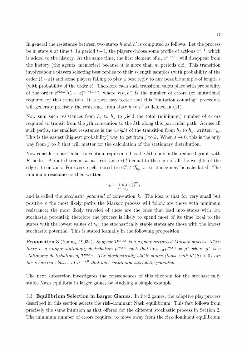
Figure 6. A Game with no Risk-Dominant Equilibrium.
In this game, the equilibrium (b, b) risk-dominates the equilibrium (a, a), whilst (c, c) risk-
dominates (b, b), but (a, a) risk-dominates (c, c). There is a cycle in the risk-dominance
relation. Clearly, since there is no “strictly” risk-dominant equilibrium, the stochastically
stable equilibrium cannot be risk-dominant.
Even when there is an equilibrium that risk-dominates all the others it need not be stochas-
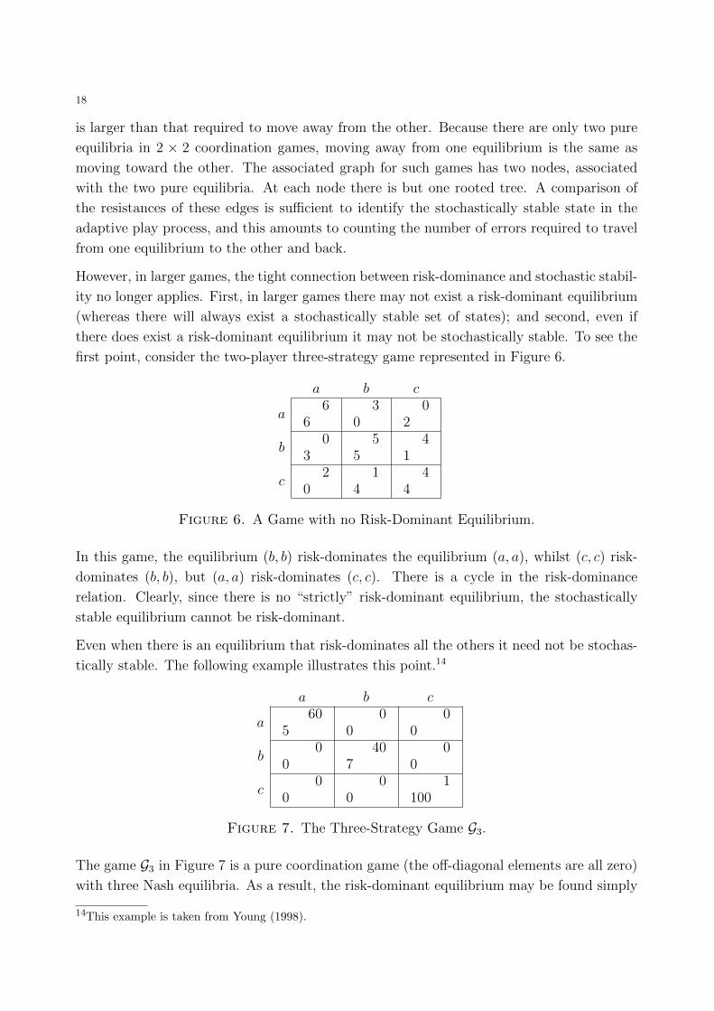
tically stable. The following example illustrates this point.14
a b c
a160
5100
0100
0
b100
0140
7100
0
c100
0100
01
100
Figure 7. The Three-Strategy Game G3.
The game G3 in Figure 7 is a pure coordination game (the off-diagonal elements are all zero)
with three Nash equilibria. As a result, the risk-dominant equilibrium may be found simply
14This example is taken from Young (1998).

19
by comparing the products of the payoffs of each of the equilibria. Therefore, (a, a) is strictly
risk-dominant (it risk-dominates both (b, b) and (c, c)).
To identify the stochastically stable equilibrium, it is necessary to compute the resistances
between the various states in the reduced graph with nodes ha, hb, and hc corresponding to
the three equilibria. Node ha represents the state ha = ((a, a), . . . , (a, a)) and so on. There
is a directed edge between each of these nodes. The graph is drawn in Figure 8.
......................................................................................................................................................................................................................................................................................................................................................................................................................................................................................................................................................................................................................................................................................................................................................
.................................................................................................................................................................................................................................................................................................................................................................................................................................
....................
......................
..........................
....................................
...................................................................................................................................................................................................................................................................................................................................................................................................................................................................................................................................................................................................................................................................................................................................................................................................................
................................................................................................................................................................................................................................................................................................................................................................•
• •
J I
I
J
I J
ha
hc hb
161
512
7107
121
25
141
Figure 8. Reduced Resistances in the Game G3.
The numbers on the directed edges in Figure 8 represent the “reduced” resistances of transit-
ing to and from the various conventions. These are calculated by considering the least costly
path between the states. Consider for example the resistance of transiting from ha to hb. In
ha players 1 and 2 will certainly receive a sample containing s copies of (a, a). Thus, to move
away from ha requires at least one of the players to err (with probability ε). Suppose this is
player 1, and that player 1 plays b instead. In the next period player 2 may receive a sample
of length s that contains 1 instance of player 1 playing b. For large s this will not be enough
for player 2 to find it a best reply to play b. Suppose player 1 again errs and plays a further
b. To optimally play b, player 2 requires at least a proportion p∗ of the s-length sample to
contain b choices, where p∗ is found from 60(1− p∗) = 40p∗. Thus p∗ = 35. Given an s-length
sample, there needs to be at least 3s/5 errors by player 1 for player 2 ever to choose b as a
best reply to some sample. Of course there are other routes out of convention ha and into
convention hb. For example, there could be a string of errors by player 2. Player 1 finds it
optimal to play b if the sample s contains at least 5s/12 errors where player 2 has played b.
Equally there could be a combination of player 1 and player 2 errors in each period. The key
is to find the least costly route: clearly these latter paths from ha to hb involve at least as
many errors as the first two “direct” paths, and so play no role as ε→ 0. Rather (ignoring

20
integer issues), the resistance from ha to hb is given by
rab = min
{5s
12,3s
5
}=
5s
12.
Ignoring the sample size s, the “reduced” resistance is 512
as illustrated in Figure 8. Similar
calculations can be made for each of the other reduced resistances. The next step is to
compute the minimum resistance rooted trees at each of the states. Consider Tha for example.
Tha = {[(hb, ha), (hc, hb)], [(hb, ha), (hc, ha)], [(hb, hc), (hc, ha)]}.
Label these rooted trees T1, T2, and T3 respectively. Then r(T1) = 141
+ 25, r(T2) = 1
61+ 2
5,
and r(T3) = 7107
+ 161
. Hence
γa = min {r(T1), r(T2), r(T3)} = 7107
+ 161.
In the same way, the stochastic potential for states hb and hc may be calculated: γb = 121
+ 141
and γc = 121
+ 7105
. Now γb = mini∈{a,b,c} γi, so (b, b) is stochastically stable. It is clear
therefore, that the stochastically stable equilibrium need not be risk-dominant, and that the
risk-dominant equilibrium need not be stochastically stable.
Nevertheless, a general result does link risk-dominance with stochastic stability in 2-player
games. Maruta (1997) shows that if there is a globally risk-dominant equilibrium, then it
is stochastically stable. Global risk-dominance requires more than strict risk-dominance: in
particular, a globally risk-dominant equilibrium consists of strategies (a1, a2) such that ai is
the unique best reply to any mixture that places at least probability 12
on aj, for i, j = 1, 2.15
Results can be proven for wider classes of games as the next proposition illustrates.
Proposition 4. Suppose G is an n-player pure coordination game. Let Pm,s,ε be the adaptive
process. Then if s/m is sufficiently small, the process Pm,s,0 converges with probability one
to a convention from any initial state h0, and the coordination equilibrium (convention) with
minimum stochastic potential is stochastically stable.
Similar results are available for other classes of game, including potential games and, more
generally, weakly acyclic games (Young, 1998).
This framework does not always imply that the dynamics select among the pure Nash equi-
libria. Indeed there are quite simple games in which they select a cycle instead of a pure
Nash equilibrium. We can illustrate this possibility with the following example.
In the game in Figure 9, (D,D) is the unique pure Nash equilibrium. It also has the following
best reply cycle:
(C,A)→ (C,B)→ (A,B)→ (A,C)→ (B,C)→ (B,A)→ (C,A).
We claim that the adaptive process Pm,s,ε selects the cycle instead of the equilibrium when
the sample size s is sufficiently large and s/m is sufficiently small. The reason is that it
15This is equivalent to the notion of p-dominance described in Morris, Rob, and Shin (1995) with p = 12 .

21
A B C D
A3
31
44
1−1
−1
B4
13
31
4−1
−1
C1
44
13
3−1
−1
D−1
−1−1
−1−1
−10
0
Figure 9. A Game with a Best-Reply Cycle.
takes more errors to move from the cycle to the basin of attraction of the equilibrium than
the other way around. Indeed suppose that the process is in the convention where (D,D)
is played m times in succession. To move into the basin of the cycle requires that someone
choose an action other than D, say C, ds/6e times in succession. Assuming that s is small
enough relative to m, the process will then move into the cycle with positive probability
and no further errors. By contrast, to move from the cycle back to the equilibrium (D,D),
someone must choose D often enough by mistake so that D becomes a best reply for someone
else. It can be verified that it is easiest to escape from the cycle when A, B, and C occur
with equal frequency in the row (or column) player’s sample, and D occurs 11 times as
often as A, B, or C. In this case it takes at least d11s/14e mistaken choices of D to transit
from the cycle to (D,D). Hence there is greater resistance to moving from the cycle to
the equilibrium than the other way around, from which one can deduce that the cycle is
stochastically stable.
More generally this example shows that selection can favour subsets of strategies rather than
single equilibria; moreover these subsets take a particular form known as minimal curb sets
(Basu and Weibull, 1991). For a further discussion of the relationship between stochastic
stability and minimal curb sets see Hurkens (1995) and Young (1998, Chapter 7).
4. Bargaining
We now show how the evolutionary framework can be used to derive Nash’s bargaining
solution. The reader will recall that in his original paper, Nash derived his solution from
a set of first principles (Nash, 1950a). Subsequently, Stahl (1972) and Rubinstein (1982)
demonstrated that the Nash solution is the unique subgame perfect equilibrium of a game in
which players alternate in making offers to one another. Although many would regard the
noncooperative model as more persuasive than Nash’s axiomatic approach, it is not entirely
satisfactory. A major drawback of the noncooperative model is the assumption that the
players’ utility functions are common knowledge, and that they fully anticipate the moves
of their opponent based on this knowledge. This seems rather far-fetched as an explanation
of how people would behave in everyday bargaining situations.
22
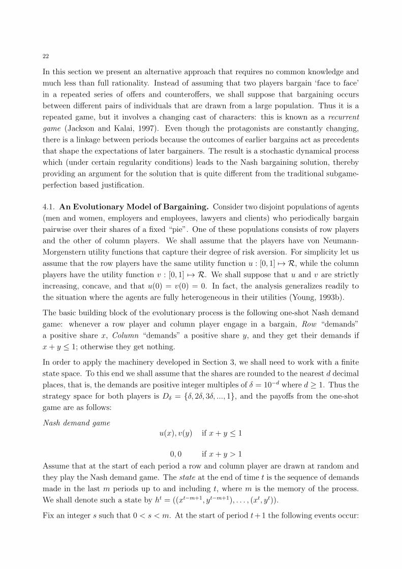
In this section we present an alternative approach that requires no common knowledge and
much less than full rationality. Instead of assuming that two players bargain ‘face to face’
in a repeated series of offers and counteroffers, we shall suppose that bargaining occurs
between different pairs of individuals that are drawn from a large population. Thus it is a
repeated game, but it involves a changing cast of characters: this is known as a recurrent
game (Jackson and Kalai, 1997). Even though the protagonists are constantly changing,
there is a linkage between periods because the outcomes of earlier bargains act as precedents
that shape the expectations of later bargainers. The result is a stochastic dynamical process
which (under certain regularity conditions) leads to the Nash bargaining solution, thereby
providing an argument for the solution that is quite different from the traditional subgame-
perfection based justification.
4.1. An Evolutionary Model of Bargaining. Consider two disjoint populations of agents
(men and women, employers and employees, lawyers and clients) who periodically bargain
pairwise over their shares of a fixed “pie”. One of these populations consists of row players
and the other of column players. We shall assume that the players have von Neumann-
Morgenstern utility functions that capture their degree of risk aversion. For simplicity let us
assume that the row players have the same utility function u : [0, 1] 7→ R, while the column
players have the utility function v : [0, 1] 7→ R. We shall suppose that u and v are strictly
increasing, concave, and that u(0) = v(0) = 0. In fact, the analysis generalizes readily to
the situation where the agents are fully heterogeneous in their utilities (Young, 1993b).
The basic building block of the evolutionary process is the following one-shot Nash demand
game: whenever a row player and column player engage in a bargain, Row “demands”
a positive share x, Column “demands” a positive share y, and they get their demands if
x+ y ≤ 1; otherwise they get nothing.
In order to apply the machinery developed in Section 3, we shall need to work with a finite
state space. To this end we shall assume that the shares are rounded to the nearest d decimal
places, that is, the demands are positive integer multiples of δ = 10−d where d ≥ 1. Thus the
strategy space for both players is Dδ = {δ, 2δ, 3δ, ..., 1}, and the payoffs from the one-shot
game are as follows:
Nash demand game
u(x), v(y) if x+ y ≤ 1
0, 0 if x+ y > 1
Assume that at the start of each period a row and column player are drawn at random and
they play the Nash demand game. The state at the end of time t is the sequence of demands
made in the last m periods up to and including t, where m is the memory of the process.
We shall denote such a state by ht = ((xt−m+1, yt−m+1), . . . , (xt, yt)).
Fix an integer s such that 0 < s < m. At the start of period t+1 the following events occur:

23
(1) A pair is drawn uniformly at random,
(2) Row draws a random sample of s demands made by column players in the history ht,
(3) Column draws a random sample of s demands made by row players in the history ht.
Let gt(y) denote the relative frequency of demands y made by previous column players in
Row ’s sample, and let Gt(y) =∫ 1
0gt(z)dz be its cumulative distribution function. Simi-
larly let f t(x) denote the relative frequency of demands x made by previous row players in
Column’s sample, and let F t(x) =∫ 1
0f t(z)dz be its cumulative distribution function.
• With probability 1− ε Row chooses a best reply, namely, xt+1 = arg max u(x)Gt(1−x). With probability ε he chooses xt+1 uniformly at random from Dδ.
• With probability 1−ε Column chooses a best reply, namely, yt+1 = arg max v(y)F t(1−y). With probability ε he chooses yt+1 uniformly at random from Dδ.
This sequence of events defines a Markov chain P ε,δ,s,m on the finite state space (Dδ)m.
A bargaining norm is a state of form hx = ((x, 1− x), . . . , (x, 1− x)) where x ∈ Dδ. In such
a state, all row players have demanded x, and all column players have demanded 1− x, for
as long as anyone can remember. The Nash bargaining norm is the state hx∗ where
x∗ = arg maxx∈[0,1]
u(x)v(1− x).
Proposition 5 (Young, 1993b). When δ is sufficiently small, s and m are sufficiently large
and s ≤ m/2, the stochastically stable bargaining norms are arbitrarily close to the Nash
bargaining norm.
Proof sketch. Fix an error rate ε, precision δ, sample size s, and memory length m satisfying
s ≤ m/2. For expositional simplicity we shall suppose that all errors are local, that is,
whenever a player makes an error it is always within δ of the true best reply. Proposition 5
continues to hold without this simplifying assumption, as shown in Young (1993b).
The first step is to calculate the number of errors it takes to exit from one norm and to
enter the basin of attraction of another. We shall illustrate this calculation with a specific
example, then pass to the more general case. Suppose that δ = 0.1 and the current norm is .3
for the row players and .7 for the column players. We shall refer to this as the norm (.3, .7).
We wish to calculate the minimum number of errors required to transit to the norm (.4, .6).
One way for such a transition to occur is that a sequence of row players demands .4 for k
periods in succession. If in the next period the current column player happens to sample all
k of these deviant demands, and if k is large enough relative to s, then she will choose .6 as
a best reply to her sample information. Indeed .6 is a best reply if v(.6) ≥ (1 − k/s)v(.7),
that is,
k ≥ [1− v(.6)/v(.7)]s (12)
Once .6 is a best reply by the column players for some sample, the process can evolve with
no further errors to the new norm (.4, .6). (This is where the assumption s ≤ m/2 is used.)
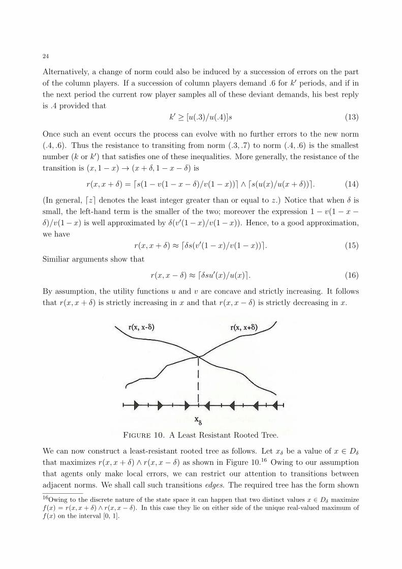
24
Alternatively, a change of norm could also be induced by a succession of errors on the part
of the column players. If a succession of column players demand .6 for k′ periods, and if in
the next period the current row player samples all of these deviant demands, his best reply
is .4 provided that
k′ ≥ [u(.3)/u(.4)]s (13)
Once such an event occurs the process can evolve with no further errors to the new norm
(.4, .6). Thus the resistance to transiting from norm (.3, .7) to norm (.4, .6) is the smallest
number (k or k′) that satisfies one of these inequalities. More generally, the resistance of the
transition is (x, 1− x)→ (x+ δ, 1− x− δ) is
r(x, x+ δ) = ds(1− v(1− x− δ)/v(1− x))e ∧ ds(u(x)/u(x+ δ))e. (14)
(In general, dze denotes the least integer greater than or equal to z.) Notice that when δ is
small, the left-hand term is the smaller of the two; moreover the expression 1 − v(1 − x −δ)/v(1− x) is well approximated by δ(v′(1− x)/v(1− x)). Hence, to a good approximation,
we have
r(x, x+ δ) ≈ dδs(v′(1− x)/v(1− x))e. (15)
Similiar arguments show that
r(x, x− δ) ≈ dδsu′(x)/u(x)e. (16)
By assumption, the utility functions u and v are concave and strictly increasing. It follows
that r(x, x+ δ) is strictly increasing in x and that r(x, x− δ) is strictly decreasing in x.
Figure 10. A Least Resistant Rooted Tree.
We can now construct a least-resistant rooted tree as follows. Let xδ be a value of x ∈ Dδ
that maximizes r(x, x + δ) ∧ r(x, x− δ) as shown in Figure 10.16 Owing to our assumption
that agents only make local errors, we can restrict our attention to transitions between
adjacent norms. We shall call such transitions edges. The required tree has the form shown
16Owing to the discrete nature of the state space it can happen that two distinct values x ∈ Dδ maximizef(x) = r(x, x + δ) ∧ r(x, x − δ). In this case they lie on either side of the unique real-valued maximum off(x) on the interval [0, 1].

25
on the x-axis of Figure 10: edges to the left of xδ point to the right, and edges to the right
of xδ point to the left. The resistance of each such edge is the smaller of the two values
r(x, x + δ), r(x, x − δ). It is straightforward to check that, among all rooted trees, this one
has least total resistance. It follows from Proposition 3 that the norm hxδ is stochastically
stable.
When δ is very small and s is very large, the value(s) xδ are very close to the unique real-
valued maximum of f(x) = u′(x)/u(x) ∧ v′(1 − x)/v(1 − x) on the interval [0, 1]. This
maximum is precisely the point x∗ where the decreasing function u′(x)/u(x) crosses the
increasing function v′(1− x)/v(1− x), that is, x∗ is the solution to
u′(x∗)/u(x∗) = v′(1− x∗)/v(1− x∗). (17)
Notice that (17) is just the first-order condition for maximizing the function ln u(x) + ln
v(1−x) on the interval x ∈ [0, 1], which is equivalent to maximizing u(x)v(1−x) for x ∈ [0, 1].
It follows that x∗ is the Nash bargaining solution. In other words, the stochastically stable
norms can be made as close as we like to the Nash bargaining solution by taking δ to be
small and s to be large.
4.2. The Case of Heterogeneous Agents. The preceding argument can be generalized
to the situation where people have different sample sizes. Suppose that the row players all
have sample size s = αm, whereas the column players all have sample size s′ = βm, where
0 < α, β < 1/2. Then expressions (15) and (16) have the following analogues:
r(x, x+ δ) ≈ dδβm(v′(1− x)/v(1− x))e, (18)
r(x, x− δ) ≈ dδαmu′(x)/u(x)e. (19)
The stochastically stable norm is determined by the crossing point of these two functions.
When m is large and δ is small this crossing point is close to the solution of the equation
αu′(x)/u(x) = β(v′(1− x)/v(1− x)),
which is the solution of
arg maxx∈[0,1]
u(x)αv(1− x)β. (20)
This is the asymmetric Nash bargaining solution. A particular implication is that, for given
utility functions, the more information that agents have (i.e., the larger their sample sizes),
the better off they are.
4.3. Extensions: Sophisticated Agents and Cooperative Games. The preceding
framework can be extended in several directions. In the version outlined above, players
do not try to anticipate what their opponents are going to do; they implicitly assume that
the opponents’ behaviour is stationary. Suppose, instead, that some positive fraction of each
population uses level-2 reasoning (Saez-Martı and Weibull, 1999): these ‘clever’ players at-
tempt to estimate what their opponent’s best reply will be, and choose a best reply to that.
26
(Thus level-2 players act as if their opponents are level-1 players.) To make such an estimate
a clever player samples the previous demands of his own population. It turns out that, if the
sample size of the clever players is at least as large as the sample size of the opponents, then
the clever agents gain nothing in the long run, that is, the stochastically stable solutions
are the same as if there were no clever agents. If, however, the clever agents’ sample size is
smaller than that of the opponents, then they do gain: the smaller sample size of the clever
agents has the same effect as reducing the sample size of the opposite population, which
reduces the latter’s relative share.
Another extension is to learning dynamics in multi-person bargaining games (Agastya, 1997)
and in cooperative n-person games (Agastya, 1999). Consider a set N = {1, 2, . . . , n} and a
value function v defined on the subsets of N that is convex and contains no dummies, that
is, for every two coalitions S and T ,
v(S) + v(T ) ≤ v(S ∪ T ) + v(S ∩ T )
and for every i ∈ N, there is some coalition Si containing i such that
v(Si − {i}) < v(Si).
There is a population of potential players for each ‘role’ i ∈ N . In each period, one agent is
drawn at random from each of the n populations. Simultaneously they make ‘demands’ and a
maximal subcoalition forms that is consistent with the demands of its members. Players not
in this coalition receive their individual payoffs v({i}). As in the bargaining model, players
draw independent random samples from the recent history and choose best replies subject
to error. The main result is that the stochastically stable demands are in the core of the
game, and these demands maximize a real-valued function that is closely related (though not
identical) to maximizing the Nash product of the players’ utilities subject to their demands
being in the core (Agastya, 1999). As in the two-person bargaining set-up, the size of a
player’s sample determines the exponent to which his utility is raised in the Nash product,
thus favouring agents with larger samples.
5. Public Goods
Public-good games often exhibit multiple Nash equilibria. The simplest example of this can
be found in any economics textbook: two agents simultaneously deciding whether to pay
for the provision of a public good. Suppose the value of the public good once provided is
positive and greater than the costs of its provision by either agent. If it takes only one of
them to provide the good, there is a coordination problem: who will provide it? If it takes
both agents to successfully generate the value associated with the public good then there
may be a different coordination problem: will it be provided or not?
Stochastic evolutionary dynamics may be applied to examine the robustness of these various
equilibria, and this section examines several such applications in precisely this context. First,
27
in Section 5.1, a very simple worked example is constructed in order to set the scene. This
requires little in the way of mathematical complexity and yields insight into the more general
results discussed in the remainder of the section. Palfrey and Rosenthal (1984) public-good
games (Section 5.2), volunteer’s dilemmas (Section 5.3), and more general public-good games
(Section 5.4) are presented in what follows.
5.1. Teamwork. Consider an n-player symmetric game in which each player i can take
one of two actions: zi = 1, interpreted as contributing toward the production of a public
good, or zi = 0 (not contributing).17 Suppose that it takes a “team” of m ≤ n individual
contributions to successfully produce the good, and generate a value of v for each player.
Any player contributing pays a cost c > 0. Thus payoffs may be written
ui(z) = v × I[|z| ≥ m]− c× zi, (21)
where z is the vector of actions (z1, . . . , zn), |z| =∑
i zi, and I is the indicator function
taking a value 1 when its argument is true, and zero otherwise. When v > c this is a discrete
public-good provision game of the kind introduced in Palfrey and Rosenthal (1984).
There are many pure-strategy Nash equilibria. For m ≥ 2, there is a Nash equilibrium
in which zi = 0 for all i: the “no-contribution” equilibrium. No player can unilaterally
deviate and do any better: the payoff received in equilibrium is zero, but any unilateral
deviation would not result in provision, and thus the deviating player would simply incur
the cost c. Any strategy profile where exactly m players contribute (so that |z| = m) is also
a Nash equilibrium: the contributing players have no incentive to deviate (each contributor
is currently receiving v − c > 0, the payoff from deviation) and every non-contributor is
receiving v > v − c, the payoff from contributing.18
Focusing on the case where v > c and m ≥ 2, there are(nm
)+ 1 pure equilibria. Which
of these are stochastically stable? In the symmetric game considered in this section, there
is no difference between any of the m-contributor equilibria, so this amounts to asking the
question: is public-good provision stochastically stable?
To answer this question, consider the following ‘one-step-at-a-time’ dynamic strategy-revision
process over the state space Z with typical member z ∈ Z. At time t a player is chosen
at random (suppose for now with uniform probability 1n) to revise their current strategy.
Suppose player i receives a revision opportunity at t and the state is currently zt = z. Player
i plays a best-reply to the current state with high probability, but plays the other strategy
with some non-zero but small probability. Concretely, suppose that conditional on z the log
17This section follows the simple example presented in Myatt and Wallace (2005) but here with the rathermore convenient logit quantal response employed in the strategy-revision process.18There are also many mixed equilibria, for a full description see Palfrey and Rosenthal (1984).

28
odds of choosing zi = 1 versus zi = 0 is linear in the payoff difference between the two:19,20
logPr[zt+1
i = 1|zt = z]
Pr[zt+1i = 0|zt = z]
= β∆ui(z), (22)
where the payoff difference is simply ∆ui(z) = ui(zi = 1; z−i) − ui(zi = 0; z−i). Note that
for β = 0 choices are entirely random, but as β →∞ choices become simple best-replies to
the current strategy profile employed by the other players z−i. In the game considered here,
∆ui(z) = v − c if |z−i| = m− 1, and ∆ui(z) = −c otherwise.
It is useful to partition the state space into “layers”. Write Zk = {z ∈ Z : |z| = k}, the
kth layer where exactly k players are contributing. The pure-strategy Nash equilibria then
are the states contained in Z0 ∪ Zm. Interest lies in the transition probabilities between the
various layers. Write pj→k = Pr[zt+1 ∈ Zk|zt ∈ Zj]. Given that a single player may conduct
a strategy revision at any time t, this probability is zero unless k and j differ by at most 1.
Suppose the state is currently in layer m−1. The process transits to the state m only if (a) a
non-contributing player is selected to revise and (b) this player chooses to contribute. Given
that m− 1 players currently contribute, n−m + 1 players do not. Thus the probability of
(a) occurring is (n−m+ 1)/n. The probability that (b) occurs is then
Pr[zt+1i = 1|zi = 0 and zt ∈ Zm−1] =
exp[β(v − c)]1 + exp[β(v − c)]
, (23)
calculated directly from (22).21 Combining these facts, the probability that the process
transits from layer m− 1 to m is
p(m−1)→m =n−m+ 1
n× exp[β(v − c)]
1 + exp[β(v − c)]. (24)
The other transition probabilities may be calculated in a similar way. The resulting Markov
process is ergodic: there is a unique distribution governing the frequency of long-run play
when t → ∞. To see this note that first, although many transitions have probability zero,
any layer may be reached from any other in finitely many positive-probability transitions and
second each layer may transit to itself (guaranteeing aperiodicity). Transition probabilities
such as (24) may be used to calculate the ergodic distribution. Write πk = limt→∞ Pr[zt ∈ Zk]for the long-run probability of being in layer k. Balance equations apply to these kinds of
finite Markov chain processes (Ross, 1996), that is,
πkpk→j = πjpj→k for all j and k. (25)
19This is a logit quantal response (McKelvey and Palfrey, 1995), and admits a random-utility interpretation.In particular, if payoffs were drawn from an i.i.d. extreme-value distribution with scale parameter β, thenthe payoff differences would be logistically distributed, and (22) would follow from a simple best-reply.20This is a common modeling choice. Indeed, later in this chapter the very same log linear construction isused in the context of games played on a network. In particular, Section 6 contains further exploration ofthis model in the discussion leading up to (and including) Proposition 7.21Note that this is a special case of the expression given in (38).

29
The ergodic distribution over layers π = (π1, . . . , πn) can then be characterized explicitly
(and for any level of β). To understand the properties of the ergodic distribution as β →∞,
in order to characterize the stochastically stable state(s) as noise is driven from the process,
it is enough to consider the ratio πm/π0. The Nash equilibria lie in layers 0 and m, and these
are the absorbing states for the noiseless process. This ratio can be calculated from a chain
of expressions such as (25) as follows
πmπ0
=
(p(m−1)→m
pm→(m−1)
)× . . .×
(p0→1
p1→0
). (26)
Notice the similarity between this exercise and the one conducted in Section 2.3. The only
difference is with the transition probabilities themselves: here they are formed from the
log linear modeling assumption made explicit in (22), whereas in the earlier section the
probabilities arose from a simple perturbed best-reply process.
Substituting in the transition probabilities found in the step above in (24) gives
πmπ0
=n−m+ 1
n
exp[β(v − c)](1 + exp[β(v − c)])
× . . .× n
n
exp[−βc](1 + exp[−βc])
/m
n
1
(1 + exp[β(v − c)])× . . .× 1
n
1
(1 + exp[−βc]). (27)
Cancelling terms and tidying up this expression gives the following result
πmπ0
=
(n
m
)exp[β(v −mc)]. (28)
The next step is to consider what will happen when noise is driven from the system (that
is β → ∞ so that players choose best-replies with probability arbitrarily close to 1). The
parameter β appears only in the exponent, and therefore the limit of the ratio in (28) is zero
if mc > v and infinite otherwise. This result is summarized in the following proposition.22
Proposition 6. Consider a symmetric n-player binary action public-good provision game
in which m ≥ 2 costly contributions are required to successfully provide the public good. Full
provision is stochastically stable if and only if the value generated to each player from the
good is greater than m times the cost to a contributing individual. When the reverse is true
the stochastically stable state involves no contributions.
All weight in the ergodic distribution is in the layer Zm whenever v > mc. The good is
provided only when the value to each individual is sufficiently large (and in particular larger
than the social cost being paid for its provision m× c). The private value needs to be larger
than the social cost. This is a point returned to in Section 5.4.
22To complete the proof, it remains to check that πk → 0 for all k 6= 0,m. This follows immediately fromsimilar calculations to those presented above in (26), (27), and (28). When k > m find πk/πm, and show itconverges to zero as β →∞; when 0 < k < m find πk/π0 and show it again converges to zero.
30
To see why this is true, rewrite this condition as v− c > (m−1)c. In order for the process to
transit from the “bottom” layer where no-one is contributing m− 1 agents must first choose
to contribute when called upon to revise even though this is not a best reply to the current
state. The final mth contributor is of course playing a best reply to the current state. The
cost to each of these players when making their choices is c. Hence the total cost of moving
up from Z0 to Zm is (m− 1)× c.
The cost of moving down is simpler: it takes but one (contributing) player to choose zi = 0.
The payoff lost to this player is v− c (0 is received instead); but once in the (m− 1)th layer,
it is now a best-reply for revising players to choose not to contribute. Thus there is just one
cost involved in moving from Zm to Z0 and it is v − c. Comparing the cost of reaching the
0th layer from the mth and vice-versa yields the result.
In this case, the ergodic distribution is analytically available. In fact, because of the con-
nection between logit quantal-response dynamics of the kind introduced here and potential
(Monderer and Shapley, 1996) the explicit form for the ergodic distribution can be used to
say much more about rather more general games (which nest the example of this section).
This will be discussed in more detail in Section 5.4.
First, though, note that in the example presented so far, symmetry was of great use during
much of the analysis; furthermore m ≥ 2 was maintained throughout. The symmetry means
the model automatically remains silent on the very first question raised in this section—who
provides the public good? Moreover, when m = 1 the game is a volunteer’s dilemma, with a
different structure (the no-contribution state no longer constitutes a Nash equilibrium) and
it is only a question of “who volunteers?” The next section relaxes the symmetry assumption
in the general m ≥ 2 case, whilst Section 5.3 examines the special case of m = 1.
5.2. Bad Apples. Abandoning the symmetric specification of Section 5.1, let each player i
receive a potentially different benefit vi from the provision of the public good, and allow the
cost a player faces when choosing zi = 1 to vary with i also (written ci). Adapting (21),
ui(z) = vi × I[|z| ≥ m]− ci × zi. (29)
This seemingly insignificant change in the model results in a game that does not admit
a potential function, the ergodic distribution is no longer explicitly available for non-zero
noise, and a rooted-tree analysis (see Section 3) is required. However, the intuition behind the
resulting characterization for the ergodic distribution as noise is driven from the stochastic
process is analogous to that described below proposition 6 above.
Assuming that vi > ci for all i, the Nash equilibria again lie in the mth layer (where
exactly m players choose to contribute) and in the 0th layer, where the public good is
not provided. These states once again are the absorbing states of a deterministic process
where in each period a player is selected at random, and chooses to play a best-reply to
the current population state. This process will eventually enter one of these two layers and,

31
once there, never leave. Now suppose that agents only probabilistically play a best-reply:
with some (high) probability an updating player selects the strategy corresponding to a best-
reply against the current population state; with some (low) probability the other strategy
is selected. Once again the question is, as the probability that a non-best-reply is selected
tends to zero, in which state does the system spend most of its time?
Myatt and Wallace (2008b) precisely characterize the ergodic distribution for vanishing noise
in such a scenario.23 To convey an idea of the content of this characterization, consider
starting in a state where all players are not contributing (the 0th layer). In order to reach
a state in which m players contribute (and thus the good is provided), the system needs to
transit “upward” to the mth layer. In order to do so, m − 1 players need to take actions
which are non-best-replies in the underlying zero-noise game. Once the (m − 1)th layer is
reached, the final step involves an updating non-contributor playing zi = 1 which, of course,
is a best-reply in the zero-noise game, and so has high probability. The first m − 1 steps
each have low probability.
In the symmetric world, each of these high cost/low probability steps entailed a cost of c on
the part of a revising player. Here, if player i revises, the associated cost is ci. Thus, the
total cost of moving up from the 0th layer to the mth layer will depend on which players bear
the cost. In line with the intuition of earlier sections it is the cheapest route which matters
for the limiting result. What is the cheapest way to reach Zm from Z0? Clearly this will
involve the m− 1 lowest-cost contributors. Ordering the players (without loss of generality)
so that c1 < c2 < . . . < cn, the total cost of moving from Z0 to Zm is simply∑m−1
j=1 cj.24
The cheapest way to transit from Zm to Z0 is more complicated. Recall that, in the symmetric
model, the cost of such a transition is simply the utility foregone from not contributing for a
revising contributor: v− c. What is the easiest way to exit from the mth layer when players
have different vs and cs? It might be conjectured initially that it is for the player with the
lowest vi − ci who is currently contributing to stop contributing. Certainly this player finds
it easiest to play zi = 0 if currently zi = 1. Two issues arise however: first, the player with
the lowest vi − ci in the population may or may not be part of the currently functioning
team; and second, there is also the possibility of exiting “upward” (a non-contributing player
could start contributing). This could be cheaper if the cost of doing so (which is greater or
equal to cm) is smaller than the cost of exiting downward (mini:zi=1 vi − ci).
These two problems have a related solution. Whereas before, in a symmetric game, it was
clear that it could not possibly be cheaper to exit via Zm+1; here that is no longer the case.
Before, such a route would inevitably involve a further transition through Zm in order to
23Myatt and Wallace (2008b) also allow for a more general class of revision dynamic, including probit-stylenoise. In the ensuing discussion here the convenient logistic specification of Section 5.1 is maintained.24Note that this leaves the process in a subset of states in Zm. In fact, it is the set defined by z ∈ Zm suchthat zi = 1 for the m − 1 lowest cost contributors (i = 1, . . . ,m − 1). One other player j > m − 1 is alsocontributing—the identity of this player does not affect the cost of transiting out of Z0.

32
reach Z0, and therefore involve an additional (but identical) cost v − c of transiting down
to Zm−1; here there may be a cheaper route involving a current non-contributor choosing
zi = 1 before another player (costlessly) ceases contributing. The point is that, in this new
state in Zm, player i has replaced one of the other contributors: this could make it cheaper
to transit to Z0 if vi − ci is particularly low. In particular, it may be possible to (cheaply)
“shoehorn” in a player from outside the current set of contributors who has a low vi − ci
before making the necessary transition down to Zm−1.
To be concrete, suppose the process is in a state z† ∈ Zm. The cheapest “direct” route to
Z0 involves a player i with zi = 1 ceasing to contribute (moving the state to Zm−1). vi − ciindexes the difficulty of this move. Now consider the “indirect” route via Zm+1. Player j,
currently a non-contributor in state z†, chooses to contribute (at a cost of cj); another player
ceases contributing at no cost; from the new state in Zm, player j stops contributing at a
cost of vj − cj. The total cost of this route out of z† is therefore cj + (vj − cj) = vj. This
is cheaper than the direct route out of z† if vj < vi − ci. It is now clear that if ci = c and
vi = v for all i this inequality can never hold. But in the absence of such symmetry there
can be a cheaper route out of Zm than the obvious direct route.
Thus, in the asymmetric version of the game, a new and interesting feature arises. The
successful provision of a public good will depend not only on the private costs and values of
those contributing, but also on the costs and values that exist in the population as a whole.
Suppose there is a player with a particularly low valuation for the public good. Even if
that player is not directly involved in public-good production (perhaps because their cost
of doing so is relatively high) their presence in the population alone may destabilize an
otherwise successfully operating team—this player is a “bad apple”.
Whilst the stochastic stability of the production equilibria versus the no-production equilib-
rium will turn on a comparison of the exit costs from Z0 and those from Zm, there is also the
question of which team of contributors is most likely to produce the public good when it is
successfully provided. In the symmetric game, this question was moot. Here, it would seem
intuitive that the m − 1 lowest-cost contributors would be involved (these players pay the
costs involved in building the “cheapest team”);25 but this leaves open the identity of the
mth contributor. As might be guessed from the above discussion, the answer to this question
depends on the distribution of costs and valuations across the whole set of players. Whilst
the full details are described in Myatt and Wallace (2008b, Theorem 1), a similar intuition
emerges from the slightly different setting of the volunteer’s dilemma, discussed next.
5.3. The Volunteer’s Dilemma. So far the public good games discussed have involved a
coordination problem of “no provision” versus “provision”. In the payoff structure given in
(29), this requires m ≥ 2. When m = 1 the game is a volunteer’s dilemma. It takes one, and
25It is not quite this obvious however, as it may be that these m− 1 include some very low-valuation (andhence relatively likely to stop contributing) players. Nevertheless, as Myatt and Wallace (2008b) show, theseplayers are in fact always involved in any successful team.
33
only one, player to contribute toward the production of the public good in order for it to be
successfully provided. So long as the maintained assumption that vi > ci for all i continues
to hold, there are n (pure) Nash equilibria, each involving zi = 1 for precisely one player i,
and zj = 0 for all j 6= i. There is no equilibrium in Z0 any longer, as (any) single player
would wish to deviate and receive vi − ci > 0. Thus all the (pure) equilibria lie in the first
layer, Z1. The only issue is “who volunteers?” Therefore the volunteer’s dilemma provides
a simple framework in which to analyze this particular element of the coordination problem
(which is nonetheless present in the case of m ≥ 2 discussed in Section 5.2).
Myatt and Wallace (2008a) provide a full analysis: once again, here the intuition behind the
results will be discussed without introducing too much formality. Again the stochastically
stable state will depend upon the ease with which various equilibrium states are exited.
These costs of exit are relatively straightforward to calculate in the m = 1 case. In each
equilibrium there are two different exit routes available. The single player who is contributing
(say i) might choose to cease doing so (at a cost of vi− ci in foregone utility). Alternatively
another player j 6= i may choose to contribute, bearing an additional cost cj. The cost of the
cheapest exit from the equilibrium in which i contributes is therefore min[(vi−ci),minj 6=i cj].26
Identifying the stochastically stable states boils down to a comparison of these exit costs
across the n states in Z1: whichever of these is the most expensive to exit is played with
probability arbitrarily close to 1 as β →∞.
It is tempting to think that, in a volunteer’s dilemma, the player with the lowest cost of
contribution ought to be the one providing the good. After all, in every equilibrium the total
gross social value generated is the same, and equal to∑
j vj. The cost paid is simply the
cost associated with the lone contributor ci. Thus net social benefit is maximized when the
player with the smallest ci (the most enthusiastic player) contributes. Indeed, if vi = v for
all i this will be the case: recall that (without loss of generality) c1 < c2 < . . . < cn, then
maxi
[vi − ci] = maxi
[v − ci] = v − c1 and minj 6=i
cj = c1 if i 6= 1 and minj 6=1
cj = c2. (30)
Escaping from the equilibrium in which the most enthusiastic player (i.e. player 1) contributes
has a cost of C1 = min[(v − c1), c2]; escaping from any other equilibrium with player i 6= 1
contributing has cost Ci = min[(v − ci), c1]. The larger of these two numbers is always C1.
Suppose v − c1 > c2. Now c2 > c1 by definition, so c2 is certainly bigger than the minimum
of c1 and any other number. Suppose c2 > v − c1. Now v − c1 > v − c2 by (30), and hence
v − c1 > min[v − c2, c1]. Thus C1 > Ci for all i 6= 1. The stochastically stable equilibrium
involves the contribution of player 1, the most enthusiastic player.
This need not be the case however. When vi 6= vj for all i and j, the most enthusiastic
player (player 1) need not be the most “reliable”: the player with the lowest ci does not
26Again, the focus here is on the logit best-reply dynamic introduced in Section 5.1. Myatt and Wallace(2008a) allow for a general range of state-dependent (Bergin and Lipman, 1996) updating rules characterizedby a pair of probabilities (indexed by some noise parameter ε) for each player.

34
also necessarily have the highest vi − ci. Suppose that player r is the most reliable: r =
arg maxi[vi−ci]. Then the stochastically stable state certainly involves zr = 1 if vr−cr < c1.
To see this, note that in such a circumstance, all the costs of moving up a layer are larger
than all the costs (foregone utilities) of moving down a layer: the easiest way to exit any
equilibrium involves the contributor ceasing to contribute. It is therefore hardest to leave
the state where r contributes.27
More enthusiastic players will contribute in the stochastically stable equilibrium the more
strongly (negatively) associated are the terms ci and vi − ci across the player set. If it were
possible to shift value from high cost players to low cost players, then doing so would reduce
the cost paid in the stochastically stable state (by ensuring that a more enthusiastic player
is contributing in the selected equilibrium).
A similar feature arises in the case when m ≥ 2 analyzed in Section 5.2. The mth player’s
identity in a selected provision equilibrium will depend not only on the costs of provision in
the pool of players, but also on the “reliability” of the players in the population.
5.4. General Public-Good Games and Potential. Further progress can be made for
more general public-good games when restricting (a) to the logit dynamics which have been
the focus of this section so far and (b) to games that exhibit potential. Blume (1997) provided
an early discussion of the relationship between potential games and log-linear choice rules.
He observed that balance equations of the kind used in (25), for example, are satisfied if and
only if the game admits an exact potential function.
To that end consider a general n-player public-good game in which each player i picks an
action zi from a finite set. Suppose that there is a player-specific cost associated with each
zi, written ci(zi). Moreover, a payoff G(z) which depends upon the vector z of every player’s
action accrues to all players. Thus a player i’s payoff may be written
ui(z) = G(z)− ci(zi), (31)
so that G(z) represents the common payoff obtained by each player and ci(zi) represents a
private payoff to i alone. The additive separability of these two components is important,
as such a game has exact potential (Monderer and Shapley, 1996). To see this, recall that
a game has exact potential if and only if there exists a real-valued function ψ such that
ui(z) − ui(z′) = ψ(z) − ψ(z′) for all z and z′ that differ by only the action of player i. In
other words, ψ is a single function which captures all of the essential strategic properties of
the game—whenever a single player i deviates from a given strategy profile z, the change in
i’s payoff is given by the change in potential.
27The remaining more complex parameter configurations are dealt with in Myatt and Wallace (2008a), whichalso contains a formal statement of the result in the following paragraph and other comparative statics.
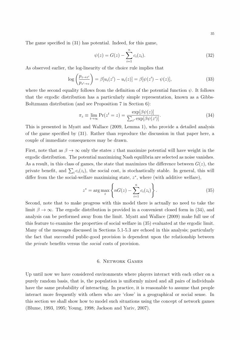
35
The game specified in (31) has potential. Indeed, for this game,
ψ(z) = G(z)−n∑i=1
ci(zi). (32)
As observed earlier, the log-linearity of the choice rule implies that
log
(pz→z′
pz′→z
)= β[ui(z
′)− ui(z)] = β[ψ(z′)− ψ(z)], (33)
where the second equality follows from the definition of the potential function ψ. It follows
that the ergodic distribution has a particularly simple representation, known as a Gibbs-
Boltzmann distribution (and see Proposition 7 in Section 6):
πz ≡ limt→∞
Pr(zt = z) =exp[βψ(z)]∑z′ exp[βψ(z′)]
. (34)
This is presented in Myatt and Wallace (2009, Lemma 1), who provide a detailed analysis
of the game specified by (31). Rather than reproduce the discussion in that paper here, a
couple of immediate consequences may be drawn.
First, note that as β →∞ only the states z that maximize potential will have weight in the
ergodic distribution. The potential maximizing Nash equilibria are selected as noise vanishes.
As a result, in this class of games, the state that maximizes the difference between G(z), the
private benefit, and∑
i ci(zi), the social cost, is stochastically stable. In general, this will
differ from the the social-welfare maximizing state, z∗, where (with additive welfare),
z∗ = arg maxz
{nG(z)−
n∑i=1
ci(zi)
}. (35)
Second, note that to make progress with this model there is actually no need to take the
limit β →∞. The ergodic distribution is provided in a convenient closed form in (34), and
analysis can be performed away from the limit. Myatt and Wallace (2009) make full use of
this feature to examine the properties of social welfare in (35) evaluated at the ergodic limit.
Many of the messages discussed in Sections 5.1-5.3 are echoed in this analysis; particularly
the fact that successful public-good provision is dependent upon the relationship between
the private benefits versus the social costs of provision.
6. Network Games
Up until now we have considered environments where players interact with each other on a
purely random basis, that is, the population is uniformly mixed and all pairs of individuals
have the same probability of interacting. In practice, it is reasonable to assume that people
interact more frequently with others who are ‘close’ in a geographical or social sense. In
this section we shall show how to model such situations using the concept of network games
(Blume, 1993, 1995; Young, 1998; Jackson and Yariv, 2007).

36
Consider a set of agents who are located at the vertices of a graph. We shall assume that the
edges are undirected, and each edge has a weight (a nonnegative real number) that measures
the importance of that particular interaction. For example, agents who are geographically
close might have higher weights than those who are far apart. Let V denote the set of n
vertices, and let i ∈ V denote a particular vertex, which we shall identify with the agent
located at i. Let wij ≥ 0 be the weight corresponding to the pair {i, j}. (If wij = 0 there is
no edge between i and j, that is, they do not interact.) We shall assume that the importance
of any interaction is weighted equally for the two individuals involved, that is, wij = wji.28
Let X be a finite set of strategies or actions, which we shall suppose is the same for each
agent. Let G be a symmetric two-person game with utility function u : X × X → R, that
is, u(x, y) is the payoff to an x-player when his opponent plays y. Let Γ be an undirected
weighted graph with n vertices. Such a network is fully described by an n-vector of weights→w ∈ Rn
+. Given G and→w, the associated network game is the n-player game defined as
follows. The joint action space is Xn. Given a profile of actions→x ∈ Xn the interactive
payoff to i is defined to be
Ii(→x) =
∑j 6=i
wiju(xi, xj). (36)
In other words, the payoff to i is the sum of the payoffs when i interacts once with every other
player, weighted by the importance of these interactions. (We remark that if the weights
at each vertex sum to one, then wij can be interpreted as the probability of the interaction
i↔ j, and Ii(→x) is the expected payoff to i.)
This framework can be extended to include idiosyncratic differences in agents’ tastes for
particular actions, a generalization that is quite useful in applications. Let vi : X 7→ Rdenote the idiosyncratic payoff that agent i would receive from taking each action in isolation,
irrespective of what the others are doing. Agent i’s total payoff from playing action xi is the
sum of the idiosyncratic payoff from xi plus the interactive payoff from playing xi given the
choices of all the other agents:
Ui(→x) =
∑j 6=i
wiju(xi, xj) + vi(xi). (37)
Consider the following example: let X be a set of communication technologies, such as
different types of cellphones. The weight wij is the frequency with which i and j communicate
per unit time period. The number u(x, y) is the payoff to someone using technology x when
communicating once with someone using technology y. The number vi(x) is the per-period
utility to agent i from owning technology x, which is determined by ease of use, cost, and
other factors that may be particular to i. Thus in state→x, the total utility to i per unit time
period is given by expression (36).
28In practice influence may be asymmetric, that is, agent i may weight j’s actions more heavily than jweights i’s actions. This situation substantially complicates the analysis and we shall not pursue it here.

37
Let us consider how such a system of n interacting agents might evolve over time. Assume
that time is discrete: t = 0, 1, 2, 3, . . . The state at time t is denoted by→xt, where
→xit∈ X
represents agent i’s choice at that point in time. At the start of each period one agent is
drawn at random and he reconsiders his choice. This is called a revision opportunity.29 As in
Section 5 we assume that whenever agent i has a revision opportunity, he chooses an action
according to a log linear response function, that is, the probability that i chooses action x
in period t+ 1 given that the current state is→xt, is given by the expression
Pr(xt+1i = x | xt) =
exp[βUi(x, xt−1−i )]∑
y∈X exp[βUi(y, xt−1−i )]
for some β ≥ 0. (38)
The number β is the response parameter. The larger β is, the more likely it is that the agent
chooses a (myopic) best response given the state→xt. This is a standard model in the discrete
choice literature (McFadden, 1976) and it can be estimated empirically from a regression
model of form30
log Pr(xti = x | xt−1)− log Pr(xti = y | xt) = β[Ui(x, xt−1−i )− Ui(y, xt−1
−i )] + εti. (39)
The stochastic adjustment process described above can be represented as a finite Markov
chain on the state space Xn. This process is irreducible—it transits from any given state
to any other state in finite time with positive probability—hence it has a unique stationary
distribution µβ. For each→x ∈ X, µβ(x) represents the long-run relative frequency with
which state x is visited starting from any initial state. In the present case this distribution
takes a very simple form. Define the function
ρ(→x) = (1/2)
∑1≤i,j≤n
wiju(xi, xj) +∑
1≤i≤n
vi(xi).
We claim that ρ(·) is a potential function for the network game. To establish this it suffices
to show that for every agent i, the change in i’s utility from a unilateral change in strategy
is identical to the induced change in potential. Fix an agent i and a set of choices by the
other agents, say→x−i. The difference in i’s utility between choosing x and choosing y is
Ui(x,→x−i)− Ui(y,
→x−i) =
∑j 6=i
wij(u(x, xj)− u(y, xj)) + vi(x)− vi(y)
= ρ(x,→x−i)− ρ(y,
→x−i).
29An analogous process can be defined in continuous time as follows. Suppose that each agent i’s revisionopportunities are governed by a Poisson random variable ωi with arrival rate λ = 1, and that the ωt’s arei.i.d. With probability one no two agents revise at exactly the same time. Hence the distinct times at whichagents revise define a discrete-time process as assumed in the text.30Note that this model appears earlier in this chapter—compare (22) with (39)—this is a very commonmodeling choice in the stochastic evolutionary game-theoretic literature following the work of Blume (1993,1995) particularly.
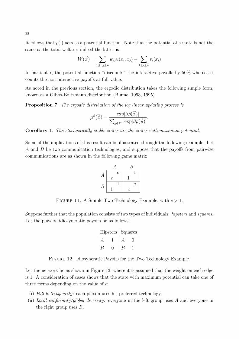
38
It follows that ρ(·) acts as a potential function. Note that the potential of a state is not the
same as the total welfare: indeed the latter is
W (→x) =
∑1≤i,j≤n
wiju(xi, xj) +∑
1≤i≤n
vi(xi)
In particular, the potential function “discounts” the interactive payoffs by 50% whereas it
counts the non-interactive payoffs at full value.
As noted in the previous section, the ergodic distribution takes the following simple form,
known as a Gibbs-Boltzmann distribution (Blume, 1993, 1995).
Proposition 7. The ergodic distribution of the log linear updating process is
µβ(→x) =
exp[βρ(→x)]∑
y∈Xn exp[βρ(→y )]
.
Corollary 1. The stochastically stable states are the states with maximum potential.
Some of the implications of this result can be illustrated through the following example. Let
A and B be two communication technologies, and suppose that the payoffs from pairwise
communications are as shown in the following game matrix
A B
Ac
c1
1
B1
1c
c
Figure 11. A Simple Two Technology Example, with c > 1.
Suppose further that the population consists of two types of individuals: hipsters and squares.
Let the players’ idiosyncratic payoffs be as follows:
Hipsters Squares
A 1 A 0
B 0 B 1
Figure 12. Idiosyncratic Payoffs for the Two Technology Example.
Let the network be as shown in Figure 13, where it is assumed that the weight on each edge
is 1. A consideration of cases shows that the state with maximum potential can take one of
three forms depending on the value of c:
(i) Full heterogeneity : each person uses his preferred technology.
(ii) Local conformity/global diversity : everyone in the left group uses A and everyone in
the right group uses B.

39
Figure 13. A Network with Two Weakly Linked Clusters.
Hipsters are represented by dots, Squares by squares. The stochastically stable
configurations depend on the coordination payoff c.
(iii) Global conformity : Everyone uses the same technology irrespective of his personal
tastes.
When the benefits from coordination are low (c < 1/2), the most likely state is full hetero-
geneity. Note that this is not optimal: more conformity would lead to higher total utility.
However, when the benefits from coordination are sufficiently large (c > 2/3) full coordina-
tion is the most likely state and it also maximizes total utility.
Perhaps the most interesting case is the intermediate one where partial coordination results.
The logic is that society consists of two groups—left and right—who interact mainly, though
not exclusively, with members of their own group. The left group (mostly hipsters) uses
technology A even though the minority of its members prefer B, while the opposite holds
for the right group. More generally, the model predicts that within-group behaviour will
be fairly uniform but between-group heterogeneity may exist when the groups interact only
weakly with each other. In particular, within-group norms may overcome heterogeneity

40
of preferences by members of the group when the conformity motive is sufficiently strong.
This is known as the local conformity/global diversity effect (Young, 1998, ch. 10). This
effect has been documented empirically in a variety of settings, including contractual norms
in agriculture (Young and Burke, 2001), and norms of medical practice (Wennberg and
Gittelsohn, 1973, 1982; Burke, Fournier, and Prasad, 2010).
7. Speed of Convergence
A common criticism of stochastic models of equilibrium selection is that it can take an
extremely long time for a population of agents to reach the stochastically stable state. Indeed,
by definition, the stochastically stable states are those whose probability is bounded away
from zero when the noise in the adjustment process is vanishingly small. When the noise
is extremely small, however, it will take an extremely long time in expectation for enough
agents to go against the flow (choose non-best replies) in order to tip the process into the
basin of a stochastically stable state.
To take a concrete case, consider a population of 101 agents in which everyone plays everyone
else once per period, and the payoffs are given by the game shown in Figure 14.
A B
A2
20
0
B0
01
1
Figure 14. A Simple Coordination Game.
Each period one player is selected at random, and he revises his choice using a log linear
response rule with parameter β. The stochastically stable state is the one in which everyone
chooses A. Now suppose that the process starts in the ‘bad’ equilibrium where everyone
chooses B. In this state, a player with a revision opportunity will switch to A with probability
e0/(e0+e100β) ≈ e−100β. Even for moderate values of β this is an extremely improbable event.
Nevertheless, we cannot conclude that evolutionary selection is impossibly slow in large
populations. A special feature of this example is the assumption that everyone plays everyone
else in every period. A more realistic hypothesis assumption would be that, in any given
period, an agent interacts only with a few people who are ‘close’ in a geographical or social
sense. It turns out that in this situation equilibrium selection can be quite rapid (Young,
1998, 2011).
To be specific, let us assume that agents are located at the nodes of a network Γ, and that
in each period every agent plays each of his neighbours exactly once using a 2 x 2 symmetric
coordination game. Let us also assume that, whenever they have a revision opportunity,
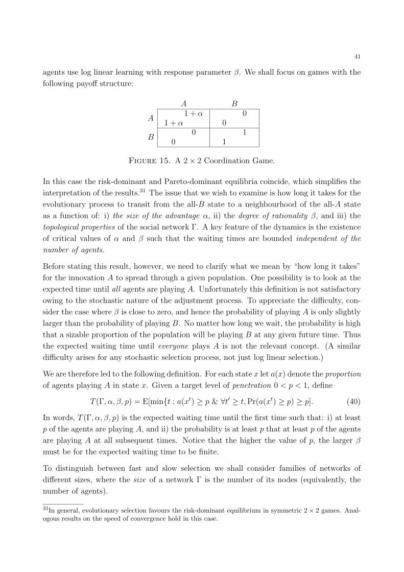
41
agents use log linear learning with response parameter β. We shall focus on games with the
following payoff structure:
A B
A1 + α
1 + α0
0
B0
01
1
Figure 15. A 2× 2 Coordination Game.
In this case the risk-dominant and Pareto-dominant equilibria coincide, which simplifies the
interpretation of the results.31 The issue that we wish to examine is how long it takes for the
evolutionary process to transit from the all-B state to a neighbourhood of the all-A state
as a function of: i) the size of the advantage α, ii) the degree of rationality β, and iii) the
topological properties of the social network Γ. A key feature of the dynamics is the existence
of critical values of α and β such that the waiting times are bounded independent of the
number of agents.
Before stating this result, however, we need to clarify what we mean by “how long it takes”
for the innovation A to spread through a given population. One possibility is to look at the
expected time until all agents are playing A. Unfortunately this definition is not satisfactory
owing to the stochastic nature of the adjustment process. To appreciate the difficulty, con-
sider the case where β is close to zero, and hence the probability of playing A is only slightly
larger than the probability of playing B. No matter how long we wait, the probability is high
that a sizable proportion of the population will be playing B at any given future time. Thus
the expected waiting time until everyone plays A is not the relevant concept. (A similar
difficulty arises for any stochastic selection process, not just log linear selection.)
We are therefore led to the following definition. For each state x let a(x) denote the proportion
of agents playing A in state x. Given a target level of penetration 0 < p < 1, define
T (Γ, α, β, p) = E[min{t : a(xt) ≥ p & ∀t′ ≥ t,Pr(a(xt) ≥ p) ≥ p]. (40)
In words, T (Γ, α, β, p) is the expected waiting time until the first time such that: i) at least
p of the agents are playing A, and ii) the probability is at least p that at least p of the agents
are playing A at all subsequent times. Notice that the higher the value of p, the larger β
must be for the expected waiting time to be finite.
To distinguish between fast and slow selection we shall consider families of networks of
different sizes, where the size of a network Γ is the number of its nodes (equivalently, the
number of agents).
31In general, evolutionary selection favours the risk-dominant equilibrium in symmetric 2× 2 games. Anal-ogous results on the speed of convergence hold in this case.

42
Fast versus slow selection. Given a family of networks G and α > 0, selection is fast for Gand α if, for every p < 1 there exists βp > 0 such that for all β ≥ βp′
T (Γ, α, β, p) is bounded above for all Γ ∈ G. (41)
Otherwise selection is slow, that is, there is an infinite sequence of graphs Γ1,Γ2, . . . ,Γn, . . . ∈G such that limn→∞ T (Γn, α, β, p) =∞.
7.1. Autonomy. We now formulate a general condition on families of networks that guar-
antees fast selection. Fix a network Γ = (V,W ), the log linear process P β, and an advantage
α > 0. Given a subset of vertices S ⊆ V, define the restricted selection process P βS as follows:
all agents i /∈ S are held fixed at B while the agents in S update according to the process
P β. Let (→AS,
→BV−S) denote the state in which every member of S plays A and every member
of V − S plays B.
Autonomy. Given a network Γ and a value α > 0, a subset S of agents is autonomous if
(→AS,
→BV−S) is stochastically stable under the restricted process P β
S . (Recall that a state is
stochastically stable if it has non-vanishing probability in the limit as β →∞.)
Proposition 8. Given a family of networks G and α > 0 suppose that there exists a positive
integer s such that for every Γ ∈ G, every member of Γ is contained in an autonomous subset
of size at most s. Then selection is fast.
In other words, given any target level of penetration p < 1, if the level of rationality β is
high enough, the expected waiting time until at least p of the agents are playing A (and
continue to do so with probability at least p in each subsequent period) is bounded above
independently of the number of the agents in the network.
Proof sketch. For each agent i let Si be an autonomous set containing i such that |Si| ≤ s. By
assumption the state (→ASi ,
→BV−Si) in which all members of Si play A is stochastically stable.
Given a target level of penetration p < 1, we can choose β so large that the probability of
being in this state after some finite time t ≥ TSi is at least 1− (1− p)2. Since this holds for
the restricted process, and the probability that i chooses A does not decrease when someone
else switches to A, it follows that in the unrestricted process Pr(xti = A) ≥ 1− (1− p)2 for
all t ≥ TSi .32 Since |Si| ≤ s for all i, we can choose β and T so that Pr(xti = A) ≥ (1− p)2
for all i and all t ≥ T . It follows that the expected proportion of agents playing A is at least
1− (1− p)2 at all times t ≥ T .
Now suppose, by way of contradiction, that the probability is less than p that at least p of
the agents are playing A at some time t ≥ T . Then the probability is greater than 1 − pthat at least 1− p of the agents are playing B. Hence the expected number playing A is less
than 1− (1− p)2, which is a contradiction.
32The last statement follows from a coupling argument, which we shall not give here. See Young (1998, Ch.6) for details.
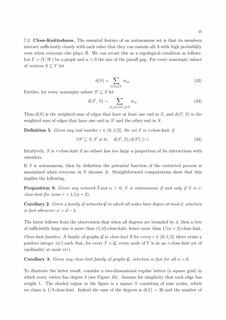
43
7.2. Close-Knittedness. The essential feature of an autonomous set is that its members
interact sufficiently closely with each other that they can sustain all-A with high probability
even when everyone else plays B. We can recast this as a topological condition as follows.
Let Γ = (V,W ) be a graph and α > 0 the size of the payoff gap. For every nonempty subset
of vertices S ⊆ V let
d(S) =∑
i∈S,j∈V
wij. (42)
Further, for every nonempty subset S ′ ⊆ S let
d(S ′, S) =∑
{i,j}:i∈S′,j∈S
wij. (43)
Thus d(S) is the weighted sum of edges that have at least one end in S, and d(S ′, S) is the
weighted sum of edges that have one end in S ′ and the other end in S.
Definition 5. Given any real number r ∈ (0, 1/2], the set S is r-close-knit if
∀S ′ ⊆ S, S ′ 6= ∅, d(S ′, S)/d(S ′) ≥ r. (44)
Intuitively, S is r-close-knit if no subset has too large a proportion of its interactions with
outsiders.
If S is autonomous, then by definition the potential function of the restricted process is
maximized when everyone in S chooses A. Straightforward computations show that this
implies the following.
Proposition 9. Given any network Γand α > 0, S is autonomous if and only if S is r-
close-knit for some r > 1/(α + 2).
Corollary 2. Given a family of networks G in which all nodes have degree at most d, selection
is fast whenever α > d− 2.
The latter follows from the observation that when all degrees are bounded by d, then a tree
of sufficiently large size is more than (1/d)-close-knit, hence more than 1/(α+ 2)-close knit.
Close-knit families. A family of graphs G is close-knit if for every r ∈ (0, 1/2) there exists a
positive integer s(r) such that, for every Γ ∈ G, every node of Γ is in an r-close-knit set of
cardinality at most s(r).
Corollary 3. Given any close-knit family of graphs G, selection is fast for all α > 0.
To illustrate the latter result, consider a two-dimensional regular lattice (a square grid) in
which every vertex has degree 4 (see Figure 16). Assume for simplicity that each edge has
weight 1. The shaded region in the figure is a square S consisting of nine nodes, which
we claim is 1/3-close-knit. Indeed the sum of the degrees is d(S) = 36 and the number of
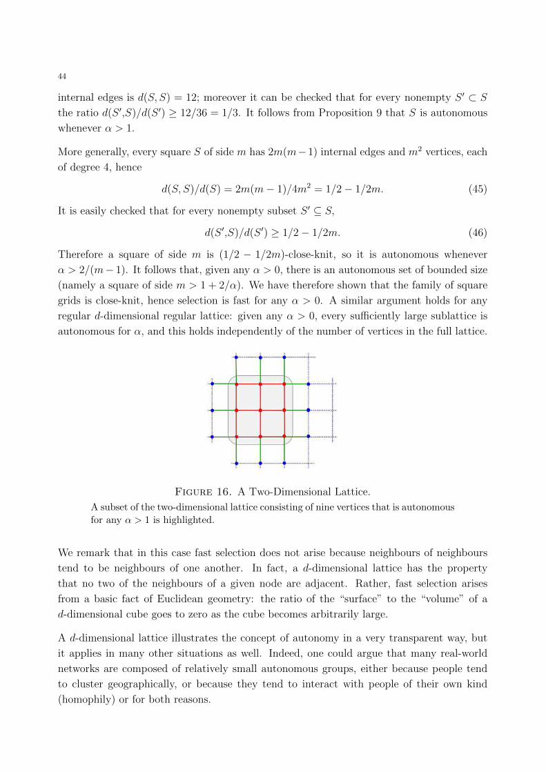
44
internal edges is d(S, S) = 12; moreover it can be checked that for every nonempty S ′ ⊂ S
the ratio d(S ′,S)/d(S ′) ≥ 12/36 = 1/3. It follows from Proposition 9 that S is autonomous
whenever α > 1.
More generally, every square S of side m has 2m(m−1) internal edges and m2 vertices, each
of degree 4, hence
d(S, S)/d(S) = 2m(m− 1)/4m2 = 1/2− 1/2m. (45)
It is easily checked that for every nonempty subset S ′ ⊆ S,
d(S ′,S)/d(S ′) ≥ 1/2− 1/2m. (46)
Therefore a square of side m is (1/2 − 1/2m)-close-knit, so it is autonomous whenever
α > 2/(m− 1). It follows that, given any α > 0, there is an autonomous set of bounded size
(namely a square of side m > 1 + 2/α). We have therefore shown that the family of square
grids is close-knit, hence selection is fast for any α > 0. A similar argument holds for any
regular d-dimensional regular lattice: given any α > 0, every sufficiently large sublattice is
autonomous for α, and this holds independently of the number of vertices in the full lattice.
Figure 16. A Two-Dimensional Lattice.
A subset of the two-dimensional lattice consisting of nine vertices that is autonomous
for any α > 1 is highlighted.
We remark that in this case fast selection does not arise because neighbours of neighbours
tend to be neighbours of one another. In fact, a d-dimensional lattice has the property
that no two of the neighbours of a given node are adjacent. Rather, fast selection arises
from a basic fact of Euclidean geometry: the ratio of the “surface” to the “volume” of a
d-dimensional cube goes to zero as the cube becomes arbitrarily large.
A d-dimensional lattice illustrates the concept of autonomy in a very transparent way, but
it applies in many other situations as well. Indeed, one could argue that many real-world
networks are composed of relatively small autonomous groups, either because people tend
to cluster geographically, or because they tend to interact with people of their own kind
(homophily) or for both reasons.

45
To understand the difference between a network with small autonomous groups and one
without, consider the pair of networks in Figure 17. The left panel shows a tree in which
every node other than the end-nodes has degree 4, and there is a “hub” (not shown) that is
connected to all the end-nodes. The right panel shows a graph with a similar overall structure
in which every node other than the hub has degree 4; however, in this case everyone (except
the hub) is contained in a clique of size 4. In both networks all edges are assumed to have
weight 1.
Figure 17. Two Networks, one with Clusters, the other without.
Every node other than the end-nodes has degree 4, and there is a hub (not shown)
that is connected to every end-node (dashed lines). All edge-weights equal 1.
Suppose that we begin in the all-B state in both networks, that agents use log linear selection
with β = 1, and that the size of the advantage is α > 2/3. Let each network have n vertices.
It can be shown that the expected waiting time to reach a state where at least 99% are playing
A is unbounded in n for the network on the left, whereas it is bounded independently of n
for the network on the right. In the latter case, simulations show that it takes fewer than
25 periods (on average) for A to penetrate to the 99% level independently of n. The key
difference between the two situations is that, in the network with cliques, the innovation can
establish a toehold in the cliques relatively quickly, which then causes the hub to switch to
the innovation also.
Note, however, that fast selection in the network with cliques does not follow from Proposi-
tion 9, because not every node is contained in a clique. In particular, the hub is connected
to all of the leaves, the number of which grows with the size of the tree, so it is not in an
r-close-knit set of bounded size for any given r < 1/2. Nevertheless selection is fast: any
given clique adopts A with high probability in bounded time, hence a sizable proportion of
the cliques linked to the hub switch to A in bounded time, and then the hub switches to
A also. In other words, fast selection occurs through the combined action of autonomy and
contagion (for further details see Young, 2011).
The preceding results show that networks with ‘natural’ topologies frequently exhibit fast
selection, but this does not mean that such topologies are necessary for fast selection. Indeed,

46
it turns out that fast selection can also occur when everyone is equally likely to interact with
everyone else, and they update based on random samples of what others are doing. To
be specific, fix a sample size d ≥ 3 and a game with advantage α > 0. Suppose that
agents revise their choices according to independent Poisson processes with expectation one.
Given a revision opportunity an agent draws a random sample of size d from the rest of the
population and chooses a log linear response with parameter β to the distribution of choices
in the sample. Let T (Γ, α, β, d) be the expected waiting time until a majority of agents
choose A, starting from the state where everyone chooses B. (Thus we are considering a
level of penetration p = 12.) We say that selection is fast for (α, β, d) if T (Γ, α, β, d) is
bounded above for all Γ ∈ G. The following result shows that selection is fast whenever α
is sufficiently large; in particular, fast selection can occur without the benefit of a particular
‘topology’.
Proposition 10 (Kreindler and Young, 2011). If agents in a large population respond to
random samples of size d ≥ 3 using log linear learning with response parameter β, selection
is fast whenever the advantage α satisfies:
α > min{(eβ−1 + 4− e)/β, d− 2} if 2 < β <∞,α > 0 if 0 < β ≤ 2.
This result shows that the dynamics exhibit a phase transition: for any given β > 2 there
is a critical level of α such that above this level the waiting time is fast, whereas below this
level the waiting time grows exponentially with the number of agents. Moreover, if β < 2
(i.e. the noise is sufficiently large), the waiting time is bounded for every positive value of α.
These waiting times are surprisingly short—on the order of 10-40 time periods—for a wide
range of parameter values. See Figure 18 which shows the waiting times for d = 4 and
various combinations of α and ε, where ε = e0/(e0 + eβ) is the probability that an agent
chooses A when everyone in his sample chooses B.
We conclude this section by pointing out some related results in the literature. Morris (2000)
studies deterministic best-response dynamics on infinite networks: in each period, each agent
myopically best responds to his neighbours’ actions. Morris identifies topological conditions
such that if the payoff gap between the equilibria is high enough, the high equilibrium spreads
by ‘contagion’ from some finite subgroup to the entire population. (This does not address
the issue of waiting times as such, but it does identify topological conditions under which the
process can escape from the low equilibrium in finite time.) A particularly interesting case
arises when the network is connected and all degrees are bounded above by some integer. In
this case α > d− 2 guarantees that a single adopter is sufficient for the innovation to spread
by contagion to the entire population. Note that this same lower bound on α guarantees
fast selection in the stochastic models discussed earlier (Proposition 9 and Corollary 2). For
related results on random networks see Lopez-Pintado (2006).

47
Figure 18. Waiting Times until 99% of the Population Plays A.
Sample size d = 4. The dashed line is the separatrix between bounded and un-
bounded waiting time.
Montanari and Saberi (2010) characterize waiting times in finite networks in terms of certain
topological properties drawn from statistical physics. As in the models of Ellison (1993) and
Young (1998, 2011) they show that local clustering tends to speed up the selection process.
They also show that small-world networks—in which most connections are ‘local’ but there
are also some links spanning long distances—tend to have much longer waiting times. It
should be noted, however, that these results are concerned with relative waiting times for
different topologies when the noise level is taken to zero (β →∞), hence the absolute waiting
times are unboundedly large. In contrast, Propositions 8-10 establish conditions under which
the absolute values of the waiting times are bounded for given values of α and β.
8. Concluding Remarks
Here we recapitulate some of the main ideas in the preceding sections. The evolutionary
framework differs conceptually from that of “classical” game theory in two major respects.
First, the focus is on large populations of individuals who interact at random, rather than on
a small number of individuals who play a repeated game. Second, individuals are assumed
to employ simple adaptive rules rather than to engage in perfectly rational behaviour. The
argument is that when many players interact randomly over long periods of time, there
is little reason to think that any one of them would have enough information to be able
to anticipate the system dynamics correctly. Moreover they have little incentive to do so,
because no one individual will have a significant influence on the future course of the process.
In this setting, an equilibrium is a rest point of the population-level dynamical process rather
than a form of consistency between beliefs and strategies, as in traditional game theory.
48
In spite of this difference in perspective, various solution concepts from traditional theory
carry over into the evolutionary setting. A case in point is ESS, which is a refinement
of Nash equilibrium. An ESS is a rest point of the dynamics that is robust to small local
deviations, that is, when given a small one-time shock, the process returns to the rest point in
question. The main contribution of stochastic evolutionary game theory is to show that this
theory must be substantially modified when the dynamical system is subjected to persistent
random perturbations. Such perturbations are quite natural and can arise from a variety of
factors, including random utility shocks, heterogeneity in payoffs, mistakes, mutations, and
so forth. These persistent perturbations typically lead to an ergodic process whose long-run
distribution can be estimated using the theory of large deviations. When these perturbations
are ‘small’ in a suitably defined sense, the ergodic distribution places high probability on
particular equilibria, which are known as stochastically stable equilibria. Thus stochasticity
injects an additional degree of realism into the models, and also leads to a sharp form of
equilibrium selection.
In this chapter we have discussed the consequences of this idea in a variety of settings,
including 2× 2 games, bargaining games, public goods games, potential games, and network
games. Another important application that we did not have the space to treat is stochastic
evolution in extensive form games (Noldeke and Samuelson, 1993; Hart, 2002). A common
theme that emerges from these cases is that stochastic stability often selects equilibria that
are well-known in traditional game theory. For example, in 2 × 2 games one obtains the
risk-dominant equilibrium, in bargaining games the Nash bargaining solution, in potential
games the potential-maximizing equilibrium, and for some classes of extensive form games
the subgame perfect equilibrium. However the justification for these solution concepts differs
between the two approaches. In traditional game theory equilibria are justified in terms of
perfect rationality, common knowledge of the game, and common knowledge of rationality,
whereas evolutionary game theory dispenses with all three of these assumptions. Nevertheless
some of the main solution concepts (or refinements of them) survive in the evolutionary
setting.
What then are the major open problems in the subject? Perhaps the single most important
challenge is to bring the predictions of theory into closer contact with empirical applications.
To date this has been attempted in relatively few cases. One example is the evolution of
contract forms in certain types of economic activity, such as agriculture. Stochastic evolu-
tionary models suggest that contract forms will tend to be more homogeneous locally than
standard theory would predict owing to positive feedback effects; moreover this prediction is
corroborated by data on contract usage in the Midwestern United States (Young and Burke,
2001). Similarly, stochastic evolutionary models can help explain the well-documented ten-
dency of medical treatments to differ substantially by geographical region (Wennberg and
Gittelsohn, 1973, 1982; Burke, Fournier, and Prasad, 2010).
49
More generally, stochastic evolutionary models provide a potentially powerful tool for an-
alyzing the dynamics of social norms. How does the structure of social interactions affect
the rate at which norms shift? Do particular interaction topologies tend to encourage lo-
cal norms or global ones? What intervention strategies are likely to be most effective for
instituting a change in norms? These questions can be studied using field data as well as
data from controlled experiments. A particularly promising direction is the field of on-line
experiments, which can be used to study the effects of interaction structure, the amount
of information available, heterogeneity in payoffs, and a variety of other factors, in a large
population setting.
References
Agastya, M. (1997): “Adaptive Play in Multiplayer Bargaining Situations,” Review of Economic
Studies, 64(3), 411–426.
(1999): “Perturbed Adaptive Dynamics in Coalition Form Games,” Journal of Economic
Theory, 89(2), 207–233.
Aumann, R. J. (1985): “What is Game Theory Trying to Accomplish?,” in Frontiers of Economics,
ed. by K. Arrow, and S. Honkapohja, pp. 28–76. Basil Blackwell, Oxford.
Basu, K., and J. W. Weibull (1991): “Strategy Subsets Closed under Rational Behavior,”
Economics Letters, 36(2), 141–146.
Bergin, J., and B. Lipman (1996): “Evolution with State-Dependent Mutations,” Econometrica,
64(4), 943–956.
Blume, L. E. (1993): “The Statistical Mechanics of Strategic Interaction,” Games and Economic
Behavior, 5(3), 387–424.
(1995): “The Statistical Mechanics of Best-Response Strategy Revision,” Games and
Economic Behavior, 11(2), 111–145.
(1997): “Population Games,” in The Economy as an Evolving Complex System II, ed. by
W. B. Arthur, S. N. Durlauf, and D. A. Lane. Westview Press, Boulder, CO.
(2003): “How Noise Matters,” Games and Economic Behavior, 44(2), 251–271.
Burke, M. A., G. M. Fournier, and K. Prasad (2010): “Geographic Variations in a Model
of Physician Treatment Choice with Social Interactions,” Journal of Economic Behavior and
Organization, 73(3), 418–432.
Ellison, G. (1993): “Learning, Local Interaction and Coordination,” Econometrica, 61(5), 1047–
1071.
(2000): “Basins of Attraction, Long Run Stochastic Stability and the Speed of Step-by-
Step Evolution,” Review of Economic Studies, 67(1), 17–45.
Foster, D., and H. P. Young (1990): “Stochastic Evolutionary Game Dynamics,” Theoretical
Population Biology, 38(2), 219–232.
(1997): “A Correction to the Paper ‘Stochastic Evolutionary Game Dynamics’,” Theoret-
ical Population Biology, 51(1), 77–78.
Freidlin, M. I., and A. D. Wentzell (1998): Random Perturbations of Dynamical Systems.
Springer-Verlag, Berlin/New York, 2nd edn.

50
Fudenberg, D., and C. Harris (1992): “Evolutionary Dynamics with Aggregate Shocks,” Jour-
nal of Economic Theory, 57(2), 420–441.
Harsanyi, John, C., and R. Selten (1988): A General Theory of Equilibrium Selection in
Games. MIT Press, Cambridge, Massachusetts.
Hart, S. (2002): “Evolutionary Dynamics and Backward Induction,” Games and Economic Be-
havior, 41(2), 227–264.
Hurkens, S. (1995): “Learning by Forgetful Players,” Games and Economic Behavior, 11(2),
304–329.
Jackson, M. O., and E. Kalai (1997): “Social Learning in Recurring Games,” Games and
Economic Behavior, 21(1–2), 102–134.
Jackson, M. O., and L. Yariv (2007): “Diffusion of Behavior and Equilibrium Properties in
Network Games,” American Economic Review, 97(2), 92–98.
Kandori, M., G. J. Mailath, and R. Rob (1993): “Learning, Mutation and Long-Run Equi-
libria in Games,” Econometrica, 61(1), 29–56.
Kreindler, G. E., and H. P. Young (2011): “Fast Convergence in Evolutionary Equilibrium
Selection,” Department of Economics Discussion Paper, 589, University of Oxford.
Lopez-Pintado, D. (2006): “Contagion and Coordination in Random Networks,” International
Journal of Game Theory, 34(3), 371–381.
Maruta, T. (1997): “On the Relationship between Risk-Dominance and Stochastic Stability,”
Games and Economic Behavior, 19(2), 221–234.
Maynard Smith, J. (1974): “The Theory of Games and the Evolution of Animal Conflicts,”
Journal of Theoretical Biology, 47(1), 209–221.
(1982): Evolution and the Theory of Games. Cambridge University Press, Cambridge.
Maynard Smith, J., and G. R. Price (1973): “The Logic of Animal Conflict,” Nature,
246(5427), 15–18.
McFadden, D. L. (1976): “Quantal Choice Analysis: A Survey,” Annals of Economic and Social
Measurement, 5(4), 363–390.
McKelvey, R. D., and T. R. Palfrey (1995): “Quantal Response Equilibria for Normal Form
Games,” Games and Economic Behavior, 10(1), 6–38.
Monderer, D., and L. S. Shapley (1996): “Potential Games,” Games and Economic Behavior,
14(1), 124–143.
Montanari, A., and A. Saberi (2010): “The Spread of Innovations in Social Networks,” Pro-
ceedings of the National Academy of Sciences, 107(47), 20196–20201.
Morris, S. (2000): “Contagion,” Review of Economic Studies, 67(1), 57–78.
Morris, S., R. Rob, and H. S. Shin (1995): “p-Dominance and Belief Potential,” Econometrica,
63(1), 145–157.
Myatt, D. P., and C. Wallace (2005): “The Evolution of Teams,” in Teamwork: An Interdis-
ciplinary Perspective, ed. by N. Gold, chap. 4, pp. 78–101. Palgrave MacMillan, New York.
(2008a): “An Evolutionary Analysis of the Volunteer’s Dilemma,” Games and Economic
Behavior, 62(1), 67–76.
(2008b): “When Does One Bad Apple Spoil the Barrel? An Evolutionary Analysis of
Collective Action,” Review of Economic Studies, 75(1), 499–527.

51
(2009): “Evolution, Teamwork and Collective Action: Production Targets in the Private
Provision of Public Goods,” Economic Journal, 119(534), 61–90.
Nachbar, J. H. (1990): “‘Evolutionary’ Selection Dynamics in Games: Convergence and Limit
Properties,” International Journal of Game Theory, 19(1), 59–89.
Nash, J. F. (1950a): “The Bargaining Problem,” Econometrica, 18(2), 155–162.
(1950b): “Non-Cooperative Games,” Ph.D. thesis, Princeton University.
Noldeke, G., and L. Samuelson (1993): “An Evolutionary Analysis of Backward and Forward
Induction,” Games and Economic Behavior, 5(3), 425–454.
Palfrey, T. R., and H. Rosenthal (1984): “Participation and the Provision of Discrete Public
Goods: A Strategic Analysis,” Journal of Public Economics, 24(2), 171–193.
Ritzberger, K., and J. W. Weibull (1995): “Evolutionary Selection in Normal-Form Games,”
Econometrica, 63(6), 1371–1399.
Ross, Sheldon, M. (1996): Stochastic Processes. Wiley, New York, 2 edn.
Rubinstein, A. (1982): “Perfect Equilibrium in a Bargaining Model,” Econometrica, 50(1), 97–
109.
Saez-Martı, M., and J. W. Weibull (1999): “Clever Agents in Young’s Evolutionary Bargain-
ing Model,” Journal of Economic Theory, 86(2), 268–279.
Sandholm, W. H. (2010): Population Games and Evolutionary Dynamics. MIT Press, Cambridge,
Massachusetts.
Stahl, I. (1972): Bargaining Theory. Stockholm School of Economics, Stockholm.
Taylor, P. D., and L. B. Jonker (1978): “Evolutionarily Stable Strategies and Game Dynam-
ics,” Mathematical Bioscience, 40(1-2), 145–156.
Weibull, J. W. (1995): Evolutionary Game Theory. MIT Press, Cambridge, Massachusetts.
Wennberg, J., and A. Gittelsohn (1973): “Small Area Variations in Health Care Delivery:
A Population-based Health Information System can Guide Planning and Regulatory Decision-
making,” Science, 182(4117), 1102–1108.
(1982): “Variations in Medical Care Among Small Areas,” Scientific American, 246(4),
120–134.
Young, H. P. (1993a): “The Evolution of Conventions,” Econometrica, 61(1), 57–84.
(1993b): “An Evolutionary Model of Bargaining,” Journal of Economic Theory, 59(1),
145–168.
(1998): Individual Strategy and Social Structure: An Evolutionary Theory of Institutions.
Princeton University Press, Princeton, New Jersey.
(2011): “The Dynamics of Social Innovation,” Proceedings of the National Academy of
Sciences, 108(4), 21285–21291.
Young, H. P., and M. A. Burke (2001): “Competition and Custom in Economic Contracts: A
Case Study of Illinois Agriculture,” American Economic Review, 91(3), 559–573.