Stochastic dominance arguments and the bounding of the generalized concave option price
42
The Journal of Futures Markets, Vol. 18, No. 6, 629–670 (1998) Q 1998 by John Wiley & Sons, Inc. CCC 0270-7314/98/060629-42 Stochastic Dominance Arguments and the Bounding of the Generalized Concave Option Price CLAUDE HENIN NATHALIE PISTRE* INTRODUCTION Nonlinear options (options whose payoff, in case of exercise, is not linear) exist under a more or less hidden form in the world of real and financial options. Classic puts on debt instruments, such as Treasury bonds and Treasury bills, can be viewed, e.g., as calls with a concave payoff—if ex- ercised—of the underlying interest rate (which is the independent state variable following a diffusion process), due to the fact that the bond price is a decreasing convex function of the interest rate. Studying calls where the payoff is a concave function of the underlying asset is thus essential to the understanding of bond call pricing. Similarly, a call (put) spread is nothing else but a call whose payoff is a concave function of the under- lying asset. Lastly, certain structures of personal taxes can transform a linear option into a concave one for the investor with an increasing mar- ginal tax rate. 1 *Correspondence author, Groupe Ceram, rue Dostolevski, BP085, 06902 Sophia Antipolis Cedex, France. 1 This remark is due to a referee. ■ Claude Henin is a Full Professor at the University of Ottawa. ■ Nathalie Pistre is a Professor in the Finance Department and Head of the Research Unit at Groupe Ceram, and associate researcher at INRIA-Sophia Antipolis.
Transcript of Stochastic dominance arguments and the bounding of the generalized concave option price

The Journal of Futures Markets, Vol. 18, No. 6, 629–670 (1998)Q 1998 by John Wiley & Sons, Inc. CCC 0270-7314/98/060629-42
Stochastic Dominance
Arguments and the
Bounding of the
Generalized Concave
Option Price
CLAUDE HENINNATHALIE PISTRE*
INTRODUCTION
Nonlinear options (options whose payoff, in case of exercise, is not linear)exist under a more or less hidden form in the world of real and financialoptions. Classic puts on debt instruments, such as Treasury bonds andTreasury bills, can be viewed, e.g., as calls with a concave payoff—if ex-ercised—of the underlying interest rate (which is the independent statevariable following a diffusion process), due to the fact that the bond priceis a decreasing convex function of the interest rate. Studying calls wherethe payoff is a concave function of the underlying asset is thus essentialto the understanding of bond call pricing. Similarly, a call (put) spread isnothing else but a call whose payoff is a concave function of the under-lying asset. Lastly, certain structures of personal taxes can transform alinear option into a concave one for the investor with an increasing mar-ginal tax rate.1
*Correspondence author, Groupe Ceram, rue Dostolevski, BP085, 06902 Sophia Antipolis Cedex,France.1This remark is due to a referee.
■ Claude Henin is a Full Professor at the University of Ottawa.
■ Nathalie Pistre is a Professor in the Finance Department and Head of the ResearchUnit at Groupe Ceram, and associate researcher at INRIA-Sophia Antipolis.

630 Henin and Pistre
Moreover, generalized options have recently appeared in “over-the-counter” financial markets, as the so-called “power options” where thereward at expiry is a power of the difference between stock price andstriking price. Hart and Ross (1994) justify the existence of nonlinearoptions by showing that the use of continuous strike options can resultin improved hedging characteristics.
In two recent articles, Henin and Pistre (1996a,b) study the case ofconvex calls and puts. A power option where the power is smaller thanone constitutes an example of a concave option, even if it is piecewiselinear. Concave calls also exist in the domain of real options. Some typesof real investments display payoffs which are concave functions of theunderlying price, because of the complex interaction of fixed and variablecharges.
The purpose of this article is to provide theoretical results aboutlower and upper bounds found on reserve buying and selling prices ofconcave European calls and puts, using second order stochastic domi-nance arguments without referring to the duplication “argument.”
Black and Scholes (1973) and Merton (1973a) have published thefundamental articles on option valuation, followed by other seminal ar-ticles on option pricing such as the ones by Harrisson and Kreps (1979),Harrisson and Pliska (1981, 1983), Karatzas (1988), and El Karoui andRochet (1989). All of these articles assume perfect and complete markets,where options can be replicated by self-financing strategies involving con-tinual revisions in a portfolio containing the underlying security. A precisevalue for the premium of the option is obtained by setting some propertiesfor the distribution of the underlying security. This allows the computa-tion of a (unique) option price through “risk-neutral” expected cash flowsdiscounted at the risk-free rate. However, the impossibility of continuoustrading due to transaction costs, or more generally the incompleteness ofthe market, is the relevant economic explanation for the opening of de-rivatives markets. Actually, when continuous trading is excluded, or withtransaction costs, Black-Scholes option prices can be generated only withvery restrictive preferences (Rubinstein, 1976; Brennan, 1979). At equi-librium derivative prices should aggregate individual demands for all theassets, especially with respect to this hedging role toward a stochasticopportunity environment, as Merton (1973b), and Cox, Ingersoll, andRoss (1985) have pointed out.
A part of the literature tries to answer these questions by consideringthat the Black-Scholes arbitrage argument is invalidated by transactioncosts (Leland, 1985; Boyle and Vorst, 1992; Jouini and Kallal, 1995).Taking a new turn, Perrakis and Ryan (1984) and Perrakis (1986) use the

Stochastic Dominance 631
equilibrium formula derived by Rubinstein (1976) to evaluate any asset;comparing three strategies involving calls, riskless assets, and stocks, theydetermine minimum necessary bounds as equilibrium values given a con-sensus on stock price distributions. Ritchken (1985) and Ritchken andKuo (1988) develop bounds for option prices based on primitive pricesin incomplete markets, where state prices are not unique, by a linearprogramming approach placing constraints on time preferences, risk aver-sion, and state probabilities.
From another literature, Hadar and Russel (1969, 1971, 1974) de-velop the notions of first- and second-degree stochastic dominance. Sec-ond-degree stochastic dominance allows the universal ranking of distri-butions among risk averse individuals. Levy and Kroll (1978) and Krolland Levy (1979) extend the use of stochastic dominance by includingriskless asset in the strategies. The notion of stochastic dominance isparticularly useful if neither the contingent claim nor the underlying assetis traded, which can be the case for real assets, for instance.
The academic community has lost interest in the concept of sto-chastic dominance, maybe because of the search for a unique price ag-gregating individual preferences (at equilibrium) or independent of thepreferences (arbitrage). However, the limits of the arbitrage arguments inincomplete markets are mentioned in the seminal article of Harrison andKreps (1979). The question of the diversity of transaction prices is a well-known issue in the microstructure literature: the existence of the spread(or of the transaction price) precludes the existence of a unique price. Inan order driven market or a price driven market, the existence of differentselling and buying prices at the same time is obvious. A traditional max-imization of the individual utility has been developed first with a hedgingpurpose (Follmer and Sondermann, 1986; Schal, 1994). Some recentworks deal with the pricing problem by determining the reserve (bid orask) price of an individual for an option he or she can trade or not. Thisapproach is employed widely in the microstructure literature, e.g., by Hoand Stoll (1981, 1983) to calculate reservation prices for a dealer. Con-stantinides and Zariphopoulou (1995) derive bounds for option pricesunder proportional transaction costs, for a (relatively) large class of utilityfunctions, by stochastic control methods using viscosity solutions. Thedisadvantage of this method is that calculations are rather tough and theyare done for special classes of utility functions.
On the contrary, the use of stochastic dominance arguments is verysimple, even with transaction costs, because there is no optimizationproblem, and the criterion is universal among risk averse individuals whensecond order stochastic dominance is used.

632 Henin and Pistre
Following Levy (1985), Henin and Pistre (1997) use this method toevaluate buying and selling reserve prices of classic European calls andfound universal bounds for risk averse buyers and sellers. For a logarith-mic Brownian motion of the underlying stock, the calculations are donefor different expectations of the mean return, and they find the spreadbetween the highest buying price and the lowest selling price, which isalways tight. The market maker is thus able to define the limits of his orher potential counterparts, which do not necessarily include the Blackand Scholes price in case of incomplete markets.
The purpose of this article is to use this methodology to derivebounds on option prices whose exercise payoff is a concave function ofthe difference between the underlying asset and striking price.
The present article develops general conditions based on second or-der stochastic arguments that such concave option prices must satisfyunder very broad assumptions, without making the hypothesis of com-plete markets, but using the hypothesis that investors are risk averse.Theoretical lower and upper bounds are derived for buying and sellingprices of concave calls and puts, and put/call “parity” relations are alsopresented.
HYPOTHESES, DEFINITIONS, ANDNOTATIONS
A generalized option on a given financial instrument (security, index, fu-ture, etc) or a real asset is an instrument that gives a reward at a givendate (expiry date), which is a function of the price of the underlyingsecurity vis-a-vis a certain price called the strike price. An option is saidto be American if this reward can be obtained before the expiry date,European if otherwise. A generalized call (put) is an option whose rewardis zero below (above) the strike price. This article focuses on the study ofa particular type of options: European, continuous concave calls and puts,i.e., options with a concave reward function.
Hypotheses
H1. The options are European options, i.e., they can only be exer-cised at expiry.
H2. The price of the underlying security is S0 at time 0. There existsfor the underlying security a probabilistic distribution of values ST at timeT, the expiration date of the options. There is no particular restriction onthe underlying distribution of the security price at time T, which is only

Stochastic Dominance 633
defined between 0 and infinity by a cumulative distribution function Fand its density function f. The expected final value of the stock and thesame expectation stopped at stock value y are defined respectively as
`
˜E (S ) 4 xf(x)dxT #0
y˜E (S ) 4 xf(x)dxy T #
0
Two other notations must be defined for values that appear in our results.The first one is the “stopped”-at-point-y expected value of the stock di-vided by the distribution function at this point. This can be viewed as themean value of the distribution until point y. The second one is the com-plementary data; it can be viewed as the mean value of the distributionafter point y:
y
xf(x)dx#0 y˜ ˜ ˜ ˜E* (S ) 4 ; E (S ) 4 E(S ) 1 E (S );y T T T y TF(y)
˜ ˜[E(S ) 1 E (S )]T y Ty* ˜E (S ) 4T [1 1 F(y)]
H3. The call is defined by a payoff function at expiry of the type: CT
4 Max(0, u(ST 1 K)), where u(0) 4 0, u8 . 0, u9 , 0; u can be apiecewise linear option. The put is defined by a payoff function of ST atexpiry of the type: Max(0, u(K 1 ST)), where u(0) 4 0, u8 , 0, u9 , 0.These reward functions also have final expected values. The same nota-tions as for the stock are defined for the call and for the put:
y`
˜ ˜E(C ) 4 u(x 1 K)f(x)dx; E (C ) 4 u(x 1 K)f(x)dx;T y T# #k K
˜ ˜E*(C ) 4 E (C )/F(y)y T y T
and
y y y˜ ˜ ˜ ˜ ˜E (C ) 4 E(C ) 1 E (C ); E * (C ) 4 E (C )/[1 1 F(y)]T T y T T T
Similarly,

634 Henin and Pistre
K K˜ ˜E(P ) 4 u(K 1 x)f(x)dx; E (P ) 4 u(K 1 x)f(x)dx;T y T# #0 y
˜ ˜E* (P ) 4 E (P )/F(y)y T y T
and
y y y˜ ˜ ˜ ˜ ˜E (P ) 4 E (P ) 1 E* (P ); E * (P ) 4 E (P )/[1 1 F(y)]T y T y T T T
H4. There exists a risk-free rate r of interest during the life of theoptions, and borrowing and lending can be made at this rate. These con-ditions are very general and do not impose a given behavior on stockprices. They just ensure the existence of finite parameters for boundingthe options. They do not preclude the existence of dividends—discrete orcontinuous—on the underlying security. Moreover, transaction costs canbe included by simply calculating the expected values of gains by takingfees into account. The hypothesis that leads all the proofs now follows.
H5. Nondominance hypothesis: If two nonlosing strategies2 have thesame cost at time 0, there cannot exist a relation of stochastic dominanceof the first or second order3 between these two strategies or a fortiori, arelation of strict dominance. This last hypothesis allows us to define min-imum conditions so that none of the two—same cost—strategies domi-nates the other, without using the hypothesis that the market is completenor the duplication of the call.
If expectations are homogeneous, bounds on the price are universal[because the SSD criterion is universal among risk averse individuals(Fishburn, 1964; Hadar and Russel, 1969; Rothschild and Stiglitz, 1970,1971)]. If expectations are heterogeneous, these bounds are subjective.
Some simple lemmas are used in the proofs of the article, the proofsof which can be found in Henin and Pistre (1997). The lemmas are re-called in Appendix A.
2It is always possible to define “losing” strategies; a losing strategy is defined as a bearish strategy ifthe expected return on the underlying security is larger than the risk-free rate, and is defined as abullish strategy otherwise.3If X and Y are two variables representing the gain of two assets, and F and G represent the cumulativedistribution functions of X and Y, respectively, F is said to stochastically dominate G at the secondorder (F SSD G) if for all t:
t t
F(x)dx # G(x)dx# #1` 1`
with a strict inequality for at least one t:
d˜ ˜⇔ Y 4 X ` g ` e
with nonpositive and E /X ` ) 4 0.g (e g

Stochastic Dominance 635
UNIVERSAL BOUNDS ON CONCAVE CALLPRICE
With no particular assumptions on the shape of the distribution and theshape of the reward function of the options, it is impossible to deriveexact formulas from hedging strategies, even if these strategies remainfeasible conceptually.
This section aims at presenting upper and lower bounds for the pre-mium at time 0 of a European concave call from comparisons betweennondominating strategies. Strategies of the same cost are now comparedto find explicit bounds which allow H5 to be verified. In order to becoherent, only strategies which are not dominated by a risk-free strategyare compared, which leads to differentiation between bullish and bearishstrategies.
In case of a bullish market, selling the asset is dominated by buyingthe asset and borrowing at the risk-free rate. Moreover, Arrow (1965)showed that all investors have a positive proportion of their wealth in-vested in the risky asset.4 To solve this problem, Levy (1985) simply sup-poses that in the Capital Asset Pricing Model framework, the asset has anonnegative beta. We prefer not to adopt this framework and to make theassumption that stock buyers make their bullish hypothesis reflected inthe present stock price and the expected return (greater than the risk-free rate), whereas sellers have the inverse expectation. The explicit hy-pothesis that buyers and sellers of the stock have different expectationsand that these expectations lead the buying prices on the one hand andthe selling prices on the other, almost “independently,” is thus made.
H5 is somewhat similar to the nonarbitrage hypothesis. Neverthe-less, to be really exploited, the latter needs the duplication of the call witha portfolio of existing instrument, which means that it needs completemarkets. Here, the markets need not to be complete. If the underlyingdistribution is not lognormal or if there are transaction costs, they are notdynamically complete. In this case, minimum conditions are defined sothat none of two strategies with the same cost dominates the other. Thereis no direct link with the notion of arbitrage, because the notion of riskis integrated in the notion of stochastic dominance. The risk is not elim-inated, as in the Black-Scholes derivation, because it is impossible. Thecalculations are never made in the so-called risk-neutral probability, butin the “real” probability. Notice that the order defined by second orderstochastic dominance is universal, if the expectations are homogeneous.If this is the case, the bounds are universal; if investors have different
4Arrow (1953) shows that if the expected return of a financial investment is larger than the risk-freerate, then every investor invests a positive proportion of his or her wealth in this asset.

636 Henin and Pistre
expectations on the distributions of the stock price, these bounds aresubjective.
Bullish Strategies
Studying bullish strategies allows us to determine bounds on buyingprices for risk averse individuals willing to buy the underlying asset and/or the call option. If the investor has the following expectation:
E(S ) . (1 ` r)S (1)T 0
then he or she adopts bullish strategies. Only bullish strategies are com-pared. Effectively, condition (1) should be satisfied for potential stock orcall buyers; if it is not satisfied, investing in the risk-free rate would sto-chastically dominate any bullish strategies on a single stock and itsoptions.
Three equal-cost strategies are defined to make some comparisonsand derive bounds on the call premium.
At time 0, strategy 1 (s1) consists in buying one unit of the under-lying security at price S0; strategy 2 (s2) consists in buying calls at priceC0 for the same amount, i.e., a quantity S0/C0; and strategy 3 (s3) consistsin buying a calls with a , S0/C0 and investing the remaining amount (S0
1 aC0) in the risk-free asset with a yield of r until expiry. The threestrategies have the same initial cost, S0.
At time T, the final value of s1 is ST, the final value of s2 is S0/C0u(ST
1 K), and the final value of s3 is au(ST 1 K) ` (S0 1 aC0)(1 ` r).
The above strategies are now compared two by two to derive condi-tions of no stochastic dominance by using H5.
Comparison 1: between s1 and s2
In order to prevent strict dominance from s1 over s2, the distributionfunctions must have at least one intersection point (see Fig. 2). As u isconcave, this implies that there exists a point at which s2 yields a largervalue than s1, which can be expressed as
S u(S 1 K)0 TMax . 131 2 4C S0 T
or

Stochastic Dominance 637
FIGURE 1Final values of s1 and s2.
u(S 1 K)TC , S Max (2)0 0 3 4SS . K TT
which gives a trivial upper bound. As u is concave and increasing, thereare one or two values of the underlying security where both strategiesgive the same final value, i.e., S0/C0u(ST 1 K) 4 ST. These points cor-respond to A and B, the intersection points of both distribution functions,of coordinates (xA, F(xA)) and (xB, F(xB)). xA and xB are the fixed pointsof the function S0/C0u(ST 1 K) as shown by Figures 1 and 2.
There is only one intersection point if
S0lim u8 (x 1 K) . 1 (3)Cx→` 0
In this case, xB is infinite. It depends, in fact, on the form of the functionu(•).

638 Henin and Pistre
FIGURE 2Distribution functions of s1 and s2.
By using the hypothesis of no dominance (H5) and lemma 1 of Ap-pendix A, it is possible to define conditions which prevent s1 from domi-nating s2. This condition, obtained at point B (B can be infinity if thereis only one intersection point), creates bounds on the call price. Noticethat despite the comparison between two distributions, there is no needto know the distribution of the underlying security, to derive theoreticalresults. Effectively, it is possible to compare state of the world by state ofthe world the respective gains of the strategies, whatever the probabilitiesof the states, because the payoffs of the option strategies depend directlyon the underlying asset value. Now s1 and s3 can be compared in thesame manner.
Comparison 2: between s1 and s3
If one compares s1 and s3, one gets the following: There can be one, two,or three intersection points, but to avoid strict dominance, the existenceof at least one intersection point is necessary. Notice that in order for s3

Stochastic Dominance 639
to lie above s1, for a final value of the underlying security equal to K, itis both necessary and sufficient to have:
(S 1 aC )(1 ` r) . K0 0
This implies that
a , (S (1 ` r) 1 K)/(C (1 ` r)) (4)0 0
This condition is impossible for options very much out of the money, i.e.,when S0 is small compared with K. For options very much in the money,it becomes feasible as the numerator increases with an increase in K andthe denominator decreases. When this condition (4) is not satisfied, thereis always one (or more) intersection points as s3 cuts s1 before value K.When this condition (4) is satisfied, there cannot be more than one in-tersection point because of the concavity of the options. In this case, asboth strategies must intersect, one must have:
au8 (`) , 1
This condition can be made as strict as possible by replacing a by itsupper bound in eq. (4) to yield:
KC . u8 (`). S 10 01 21 ` r
However, because a , S0/C0, the condition reduces to
C . u8 (`). S (5)0 0
For
(S (1 ` r) 1 K)/(C (1 ` r)) , a , S /C (6)0 0 0 0
there is at least one intersection point. There is a unique intersectionpoint if for any x . K:
(S 1 aC )(1 ` r) ` au(x 1 K) , x ⇔0 0
x 1 S (1 ` r)0a , Min (7)3 4u(x 1 K) 1 C (1 ` r)x.K 0
If this last condition is not respected, there are two intersection points if
au8 (`) . 1 (8)

640 Henin and Pistre
and three points otherwise. Setting a8, the possible values of a [verifyingeqs. (4) and (5) or eqs. (6) and (7)] such that there is a unique intersectionpoint, C(xC, F(xC)), a9 [verifying eq. (6); eq. (8) without eq. (7)] for twointersection points, C(xC, F(xC)) and D(xD, F(xD)), and finally a- [veri-fying eq. (6) without eqs. (7) or (8)] for three intersection points, C(xC,F(xC)), D(xD, F(xD)), and E(xE, F(xE)). The intersection points betweenthe final values of s1 and s3 are such that the first coordinate is a fixedpoint of the function: au(x 1 K) ` (S0 1 aC0) (1 ` r). If there is onlyone intersection point, it implies that xD is infinite and it does not in anyway affect the validity of the results obtained in the two intersectionpoints situation. Figure 3 shows the two intersection points situation inthe final payoffs and Figure 4 shows the three intersection points situa-tion. As can be seen in Figures 3 and 4, the option strategy dominates inthis case the stock strategy for small final values. Thus, the expected valueof s3 must not be too high, unless s3 dominates stochastically s1. Theconstraint is thus the inverse of the one obtained in the previous com-parison, which implies that lower price bounds are also obtained.
Theorem 1 (Proof in Appendix B)
The buying price of a concave call verifies:
˜E (C )x TBC , S (9)0 0 ˜E (S )x TB
with xB eventually infinite (if there is only one intersection point), and
˜ ˜S (1 ` r) ` a9 E* (C ) 1 E* (S )0 x T x TD DC . Max Max ;0 3 a9 (1 ` r)F(x )a9 D
˜ ˜S (1 ` r) ` a8 E(C ) 1 E(S )0 T TMax (10)4a8 (1 ` r)a8
˜ ˜S (1 ` r) ` a- E (C ) 1 E (S )0 x T x TD DC . Max Min ;0 3 a- (1 ` r)F(x )a- D
˜ ˜S (1 ` r) ` a- E(C ) 1 E(S )0 T T (11)4a- (1 ` r)
Note that the lower bound of the call premium makes the stochasticdominance of the option upon the stock impossible, while the upperbound of the call premium makes the stochastic dominance of the stock

Stochastic Dominance 641
FIGURE 3Final values of s1 and s3. Two intersection points.
upon the option impossible. To derive numerical results, it is necessaryto make some hypotheses on the underlying asset distribution. Equation(9) is then a simple computation, because the intersection point is foundeasily. Equations (10) and (11) can be calculated by iteration: Each po-tential price C0 must verify these relations and is rejected if this is notthe case. For numerical results in the “linear” case, see Henin and Pistre(1997).
Bearish Strategies
Bearish strategies involve the selling of calls or stocks. In order not to bedominated by a lend at the risk-free rate, the following inequality musthold for the seller:
E(S ) , S (1 ` r) (12)T 0
The three former strategies are dominated by an investment in the risk-

642 Henin and Pistre
FIGURE 4Final values of s1 and s3. Three intersection points.
free rate and must be replaced by the reverse (selling) strategies to obtainbounds on the selling price of the calls.
At time 0, s18 consists in selling one unit of the underlying securityat price S0, s28 in selling S0/C0 options to get initially the same amountS0, and s38 in selling a options with a , S0/C0 (for an initial amountaC0) and borrowing (S0 1 aC0) at the risk-free rate to start with thesame initial amount S0. The final values are, respectively, for s18, 1ST
with a distribution function F8, for s28, 1S0/C0•u(ST 1 K), and for s38,1au(ST 1 K) 1 (S0 1 aC0)(1 ` r).
Comparison 3: between s18 and s28
If one notices that F8(x) 4 P(1ST , x) 4 P(ST . 1x) 4 1 1 F(x),there are one or two intersection points of the same coordinates as in thebullish situation, (1xA, F(xA)) and (1xB, F(xB)) (see Figs. 5 and 6).
To understand the intuition of the results for selling prices a generalremark applies. The bearish strategies are the exact symmetry of the bull-

Stochastic Dominance 643
FIGURE 5Final values of s18 and s28. Two intersection points.
FIGURE 6Distribution functions of s18 and s28.

644 Henin and Pistre
ish strategies. However, the symmetry in the results is not trivially ob-tained. In the case of two intersection points, the strategy which tends todominate for the smallest final payoffs in the bullish case (for instance,s1 in comparison 1) is dominated (in its bearish form) for the smallestfinal payoffs in the bearish case (s18 in comparison 3). In addition, be-cause of the short positions, those smallest final payoffs are obtained forthe highest value of the underlying asset. In this case, the inequalitybetween the expected values of the two strategies is inverted, but becauseof the negative sign of the final values, the bound on the price is finallyobtained on the same side as in the bullish case. In the case of an oddnumber of intersection points, the strategy which tends to dominate forthe smallest final payoffs in the bullish case still dominates (in its bearishform) for the smallest final payoffs in the bearish case (s18 in comparison3 with only one intersection point). In this case, the inequality betweenthe expected values of the two strategies is not inverted, and because ofthe negative sign of the final values, the bound on the price is finallyobtained on the opposite side of the bullish case. In this bearish situation,an upper bound is thus obtained for the call price if there are two inter-section points in order to prevent the dominance of s28, and a lowerbound if there is one intersection price in order to prevent the dominanceof s18. Notice that the second intersection point is (1xA, F8(1xA)).
Comparison 4: between s18 and s38
Here again, to obtain at least one intersection between the strategies, toprevent strict dominance, one has the same upper bound (2) as for com-parison 2. The same three cases happen, depending on the chosen valueof a: a8, a9, a-. The previous remark applies: The bounds are obtainedon the opposite side of the bullish case except in the case of two inter-section points, where a lower bound is obtained again.
Theorem 2 (Proof in Appendix B)
The selling price of a concave call verifies:
xA ˜E (C )TC , S (13)0 0 xA ˜E (S )T
with xA infinite if there is only one intersection point. For every a8, a9,and a- defined previously:

Stochastic Dominance 645
x xC C˜ ˜S (1 ` r) ` a9 E * (C ) 1 E *(S )0 T TMax3 4a9(1 ` r)a9
˜ ˜S (1 ` r) ` a8 E(C ) 1 E(S )0 T T, C , Min (14)0 3 4a8(1 ` r)a8
x xD D˜ ˜S (1 ` r) ` a- E * (C ) 1 E * (S )0 T TC , Min Max ;0 3 a-(1 ` r)a-
˜ ˜S (1 ` r) ` a- E(C ) 1 E(S )0 T T (15)4a-(1 ` r)
In this bearish situation, the upper bound of the call premium makes thestochastic dominance of the latter upon the stock impossible (the callmust not be sold too high), while the lower bound of the call premiummakes the stochastic dominance of the stock impossible (the stock mustnot be sold too high).
BOUNDS ON CONCAVE PUT PRICE
Bounds can be obtained for concave puts as they were obtained for calls.The comparisons still use either bullish or bearish strategies dependingupon the expectation on stock returns. This implies that, in the strategies,stock buying is always associated or compared with put writing and viceversa.
In case of a bullish market, two strategies (s4 and s5) are now de-fined, which are compared successively with s1, which stays identical.The following hypothesis is made:
P , u(K)/(1 ` r) (16)0
That is, the price P0 for insurance is, of course, smaller than the certaincash flow u(K) (the best case with certitude).
Bullish Strategies
Strategy 4 (s4) consists in buying one share and buying c puts and bor-rowing cP0 with c , 1/u8(0), in order for the gains of the strategy to bestrictly monotonic. In strategy 5 (s5), one writes d puts and invests (dP0
` S0) in the risk-free asset. For
d 4 S (1 ` r)/u(K) 1 P (1 ` r) (17)0 0 0

646 Henin and Pistre
s1 and s5 have the same final value for ST 4 0, i.e., 1d0u(K) ` (d0P0
` S0)(1 ` r) 4 0. Strategy 5 is considered with d8 , d0, then with d9 .d0.
Lemma 4 (Proof in Appendix C)
The gain at point ST 4 0 decreases when d increases.The final value of s4 is cu(K 1 ST) ` cST 1 cP0(1 ` r) and the
final value of s5 is 1du(K 1 ST) ` (dP0 ` S0)(1 ` r).
Comparison 5: between s1 and s4
Because of eq. (16), the value of the gain of s4 for ST 4 0 is higher thanthe gain of s1 and there is a unique fixed point xM of the function: cu(K1 x) ` cx 1 cP0(1 ` r).
Thus, the distribution functions of s1 and s4 have a unique inter-section point, M(xM, F(xM)), and a condition in order s4 not to dominates1 can be found (see Figs. 7 and 8).
Comparison 6: between s1 and s5
For d9 . d0, there is at least one intersection point if there exists x , Ksuch as 1d9 u(K 1 x) ` (d9P0 ` S0)(1 ` r) . x, which implies thefollowing necessary condition:
x ` d9 u(K 1 x) 1 S (1 ` r)0P . Max Min (18)0 d9(1 ` r)d9.d x0
In this case, there are two and only two intersection points between thedistribution functions s1 and s5, N(xN, F(xN)) and P(xP, F(xP)), and xN
and xP are the fixed points of the function 1d9u(K 1 x) ` (d9P0 ` S0)(1` r) as shown in Figure 9.
For d8 , d0, there is at least one intersection point, but there areeither one or three intersection points, depending on the form of u(•), asshown by Figures 10 and 11.
Theorem 3 (Proof in Appendix C)
The selling price of a concave put verifies:
˜ ˜E(S ) ` d8 E(P ) 1 S (1 ` r)T r 0P , Max Min ;0 3 d8 (1 ` r)d
˜ ˜E* (S ) ` d8 E* (P ) 1 S (1 ` r)xp T xp T 0Min (19)4d8 (1 ` r)d
with xP eventually infinite if there is only one intersection point5:
5In this case, the two expressions in eq. (17) are identical.

Stochastic Dominance 647
FIGURE 7Final values of s1 and s4.
˜ ˜ ˜E* (S ) ` d9 E* (P ) 1 S (1 ` r) E(P )xp T xp T 0 TP . Max Max ; (20)0 3 4d9(1 ` r) (1 ` r)d9
Puts are sold in both s4 and s5; eq. (19) shows that they cannot be soldat too high a price to prevent the dominance of the stock buying strategyby s4 but also at a price sufficiently high (20) to prevent them from beingdominated by the stock buying strategy. In case of bearish expectations,one can make the following comparisons for selling prices.
Bearish Strategies
In this case, the following (inverse) strategies are defined. Strategy 48 (s48)can be defined but gives a trivial result. Strategy 58 (s58) consists in buyingd puts and borrowing (dP0 ` S0). This strategy with d8 , d0 and thenwith d9 . d0 is again considered. Both strategies, as well as s18, which isused for comparison, have an initial positive flow of S0. The final valueof s58 is du(K 1 ST) 1 (dP0 ` S0)(1 ` r).

648 Henin and Pistre
FIGURE 8Distribution functions of s1 and s4.
Comparison 7: between s18 and s48
This comparison is the exact symmetry of comparison 5. Thus, the dis-tribution functions of s18 and s48 have a unique intersection point,M(1xM, F8(1xM)), and a condition in order s48 not to dominate s18 canbe found. A lower bound is obtained for the buying put price.
Comparison 8: between s18 and s58
The conditions for the existence (and the number) of intersection pointsare those of comparison 6. For d9 . d, the condition (18) must be verifiedand the two intersection points of the distribution functions s18 and s58
are N(1xN, F8(1xN)) and P(1xP, F8(1xP)). For d8 , d0, there is alwaysat least one intersection point and there may be one or three intersectionpoints, depending on the form of u(•) as in the bullish strategies. Thesame general remark applies with respect to the symmetry of results (to-ward bullish results) depending on the number of intersection points.These strategies give only lower bounds on the buying price of the put.Another strategy must be defined to find an upper bound.
Strategy 68(s68) is to buy one put and sell b shares with

Stochastic Dominance 649
FIGURE 9Final values of s1 and s5 for d9 . d0.
b 4 (P ` S )/S (21)0 0 0
in order to again have an initial positive flow of S0. The final value of s68
is 1u(K 1 ST) 1 b ST.
Comparison 8: between s18 and s68
In order for s68 not to be strictly dominated by s18, there must exist x ,K such as
u(K 1 x) 1 bx . 1x
Because of the value of b defined by eq. (21), the put price must verify:
u(K 1 x)P , Min (22)0 xx
which gives a first (trivial) bound. In this case, there must be one or two

650 Henin and Pistre
FIGURE 10Final values of s1 and s5 for d8 , d0. One intersection point.
intersection points, U(1xU, F8(1xU)) and V(1xV, F8(1xV)) (see Figs.12 and 13).
Theorem 4
The buying price of a concave put verifies:
xU ˜E (P )TP , S (23)0 0 xU ˜E (S )T
with xu eventually infinite if there is only one intersection point, and
˜ ˜E(S ) ` d8 E (P ) 1 S (1 ` r)T T 0P . Max Min ;0 3 d8 (1 ` r)d8
x xP P˜ ˜E * (S ) ` d8 E * (P ) 1 S (1 ` r)T T 0Min (24)4d8 (1 ` r)d8
with xP eventually infinite, and

Stochastic Dominance 651
FIGURE 11Final values of s1 and s5 for d8 , d0. Three intersection points.
x xN N˜ ˜E * (S ) ` d9 E * (P ) 1 S (1 ` r)T T 0P . Max (25)0d9 (1 ` r)d9
All of these bearish strategies dealing with puts involve buying puts andselling stocks. The upper bound guarantees that the put does not domi-nate and the lower bound guarantees that the stock does not dominate.
A PUT/CALL RELATION
As minimum relations holding at each time between call and stock prices(or put and stock prices), minimum conditions existing necessarily be-tween call and put prices at each instant can be defined. Setting uc(x 1
K) the final gain of the call, which is null if x , K and increasing andconcave otherwise, and up(K 1 x) as the final gain of the put, which isnull if x . K and decreasing and concave otherwise. In order for the putand call to be comparable, uc(x 1 K) 4 up(K 1 x) for x 4 K ` h and

652 Henin and Pistre
FIGURE 12Final values of s18 and s68.
x8 4 K 1 h, with 0 , h , K. Two new strategies are now defined forbullish expectation.
Bullish Put/Call Bounds
Strategy 7 (s7) is to write k puts, buy k calls, and invest (kP0 1 kC0 `
S0) in the risk-free asset. This strategy has the same cost S0 as s1. Thefinal value of s7 is
for x . K; ku (x 1 K) ` (kP 1 kC ` S ) (1 ` r)c 0 0 0
for x , K: 1ku (K 1 x) ` (kP 1 kC ` S ) (1 ` r)p 0 0 0
Setting k0 such that the final gain of s7 if ST 4 0 is 0, k0 verifies:
1S (1 ` r)0k 4 (26)0 [1u (K) ` (P 1 C )(1 ` r)]p 0 0
Stochastic Dominance 653
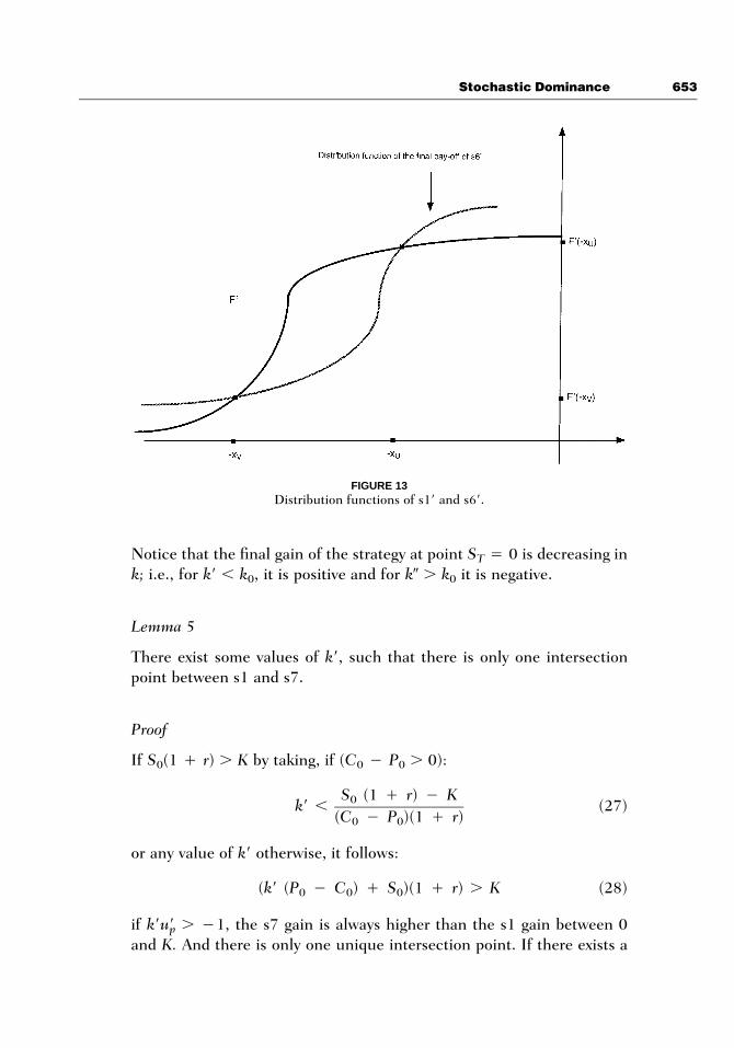
FIGURE 13Distribution functions of s18 and s68.
Notice that the final gain of the strategy at point ST 4 0 is decreasing ink; i.e., for k8 , k0, it is positive and for k9 . k0 it is negative.
Lemma 5
There exist some values of k8, such that there is only one intersectionpoint between s1 and s7.
Proof
If S0(1 ` r) . K by taking, if (C0 1 P0 . 0):
S (1 ` r) 1 K0k8 , (27)(C 1 P )(1 ` r)0 0
or any value of k8 otherwise, it follows:
(k8 (P 1 C ) ` S )(1 ` r) . K (28)0 0 0
if k8 . 11, the s7 gain is always higher than the s1 gain between 0u8pand K. And there is only one unique intersection point. If there exists a

654 Henin and Pistre
FIGURE 14Final values of s1 and s7. One intersection point.
point such that k8 is not .1, setting R the point such that 1up8(xR)u8p4 1/k, ; xR is also decreasing in k. In this case, to have one uniqueintersection point, the following inequality must hold:
S (1 ` r)0k8 , (29)u (K 1 x ) ` (C 1 P )(1 ` r)P R 0 0
If the denominator is positive or any value otherwise.If S0(1 ` r) , K, if (C0 1 P0 , 0) by taking k8 verifying:
S (1 ` r) 1 K0k8 , (30)(C 1 P )(1 ` r)0 0
or any value of k8 otherwise, it follows:
(k8 (P 1 C ) ` S )(1 ` r) , K (31)0 0 0
If k8 , 1, the s7 gain is always lower than the s1 gain for ST . K. Andu8Cthere is only one unique intersection point. If there exists a point suchas k8 is not ,1, setting R8 the point such that ( ) 4 1/k8. In thisu8 u8 x8C p R

Stochastic Dominance 655
FIGURE 15Final values of s1 and s7 for k9 . k0. Two intersection points.
case, to have one unique intersection point, the following inequality musthold:
S (1 ` r)0k8 , (32)u (K 1 x ) ` (C 1 P )(1 ` r)C R8 0 0
if the denominator is positive or any value otherwise.As illustrated in Figures 14 and 15, a constraint must hold, so that
the put/call strategy s7 does not dominate the stock strategy s1.For k9 . k0 (33), to prevent strict dominance of s1, there must exist
x such that
k9 u (x 1 K) ` (k9 (P 1 C ) ` S )(1 ` r) . x (33)c 0 0 0
x 1 S (1 ` r)0P 1 C , Min (34)0 0 u (x 1 K) ` (P 1 C )(1 ` r)x c 0 0
The following results are obtained.

656 Henin and Pistre
Theorem 5
The spread between the buying price of the call and the selling price ofthe put verifies:
˜ ˜ ˜E* (P ) 1 E*(C ) ` E*(S ) Sx T x T x T 0z z zMax 1 , P 1 C0 0(1 ` r) k9k9
˜ ˜ ˜E (P ) 1 E(C ) ` E(S ) ST T T 0, Min 1 (35)(1 ` r) k8k8
Bearish Put/Call Bounds
Defining the inverse strategy s78 [buy k puts, write k calls, and invest(1kP0 ` kC0 1 S0) in the risk-free asset] in case of bearish expectationsimplies the derivation of two lower bounds.
In order to get an upper bound, it is necessary to exhibit a strategywhich is dominated by s18 for small values of gains (very negative). Thisis possible if
1k9 . lim (36)
u8 (x 1 K)x→` c
Such a value is finite only if
lim u8 (x 1 K) ? 0 (37)cx→`
In this case, there is a unique intersection point, L(1xL; F8(1xL)), of thetwo strategies (see Figs. 16 and 17) and a constraint must be defined, sothat the stock strategy s18 does not dominate the put/call strategy s78.This comparison gives a bound on the other side.
Theorem 6
The spread between the selling price of the call and the buying price ofthe put verifies:
˜ ˜ ˜E(P ) 1 E(C ) ` E(S ) ST T T 0P 1 C . Max 1 (38)0 0 (1 ` r) k8k8
If eq. (37) is verified, by taking k9 verifying eq. (36), it follows:
˜ ˜ ˜E(P ) 1 E(C ) ` E(S ) ST T T 0P 1 C , Min 1 (39)0 0 (1 ` r) k9k9

Stochastic Dominance 657
FIGURE 16Final values of s18 and s78 for k9.
FIGURE 17Distribution functions of s18 and s78.

658 Henin and Pistre
CONCLUSIONS
The present article offers some general properties for generalized concaveoptions. All the conditions obtained depend solely on the first momentof the distributions of the options and the underlying security, withouteven including the variance. This is purely formal, as the whole distri-bution is included from the asymmetry in the reward function of theoption and from the fact that its expected value is an intrinsic part of theconstraints. When the yields are normally distributed, the Black-Scholesformula makes the variance appear explicitly. In a more general fashion,computing the expected value of the call under real probability and com-paring it with the distribution and expected value of the underlying se-curity really captures the whole distribution, any eventual asymmetry be-ing put forward by their comparison.
The bounds presented here are very general. The payment of divi-dends on the underlying security easily can be taken into account, be-cause it can be directly included in the final expected value of the stock.The payment of dividends simply affects the distribution of the stockprices at expiry, thus resulting simply in a modification of the functionu(•) to be used in the results. This is an important extension which comesfrom the fact that only final distribution of the stock price is used in thebounding conditions. Similarly, there is no difficulty in taking transactioncosts into account, since there is no duplication strategy in our method.Once again, these costs simply affect the initial cost of the strategies (inthe bullish case, S0 plus the transaction cost) and the expected payoffsof the strategies (decreased by the transaction cost).
The practical use of these results is clear even if a unique price isnot found for the option. Consider a market maker on options. This mar-ket maker is able to determine the highest price at which a bullish investorwill accept to buy the option and the lowest price at which a bearishinvestor will accept to sell the option. The bullish higher bound on theoption price can thus be calculated with respect to the actual price of theasset, i.e., the ask price of the market maker. Constraints on the spreadson options can thus be defined vis-a-vis the spreads offered on the un-derlying security by simply replacing the share price by its bid or ask price,depending on the sense of the transaction.
This represents a theoretical spread, of course, adjusted for the pur-pose of competition. In most cases, there are no analytical values of thebounds, because the various intersection points depend on the price ofthe option itself. For a given possible price of the call, one must checkthat the relations are verified. If not, one must proceed by iteration untila price is not rejected. The computations of the bounds for various con-

Stochastic Dominance 659
cave payoffs constitute a further research development. Because pricingis not the only objective of investors, one other important research de-velopment will be the derivation—analytically or numerically—of the sen-sibility of the bounds with respect to various parameters, e.g., price andvolatility of the underlying asset, and time to maturity.
APPENDIX A: LEMMAS OF SECOND ORDERSTOCHASTIC DOMINANCE
Lemma 1 (Hammond, 1974)
When there exits A(xA,F(xA)) such as
F(x) , G(x) ∀x , x , F(x) . G(x) ∀xA
. x , F(x ) 4 G(x ) (A1)A A A
(i.e., F intersects G once and only once from below at point A), F sto-chastically dominates G if and only if
E(X) $ E(Y)
Lemma 2
If
∃B(x , F(x )), and C(x , F(x ))B B c c
with 0 , xB , xC such as
F(x) , G(x) ∀x , x and x . x ; F(x) . G(x) x , x , xB c B c
F(x ) 4 G(x ) and F(x ) 4 G(x )B B C C
(i.e., F intersects G twice, first from below at point B and then from aboveat point C), F dominates G in the SSD sense if and only if
x x x xC C C C
F(x)dx # G(x)dx ⇒ xf(x)dx $ xg(x)dx (A2)# # # #1` 1` 1` 1`
i.e., if condition (A1) is satisfied at the second intersection point C.
Lemma 3
When F intersects G more than twice, the first time being from below, Fdominates G in the SSD sense if eq. (A2) is satisfied for all even-num-

660 Henin and Pistre
bered intersection points, infinity being considered such a point [i.e.,condition (A2) applies to the mean if there is an odd number of intersec-tion points].
APPENDIX B: PROOFS OF THEOREMSOBTAINED FOR CONCAVE CALLS
Proof of Theorem 1
Comparison 1
For x , xA and x . xB S0/C0u(x 1 K) , x; this implies that F(x) , G(x)and, for xA , x , xB, S0/C0u(x 1 K) . k; hence, F(x) . G(x). Thisimplies that the conditions of lemma 2 are satisfied. Thus, if (s1) $ExB
(s2), then s1 DS2 s2: hence a contradiction with H5. Therefore,ExB
E (s1) , E (s2)x xB B
which implies
S0˜ ˜E (S ) , E u(S 1 K)x t x r1 2B B C0
and thus:
˜E (C )x TBC , S0 0 ˜E (S )x TB
If there is only one intersection point, xB is infinite and this relationbecomes:
˜E (C )TC , S0 0 ˜E (S )T
From this eq. (9) is obtained.
Comparison 2
Three different cases can be obtained according to the number of inter-section points. The first two cases are similar because one intersectionpoint is equivalent to two intersection points, with the second one infi-nite. The case of two intersection points C and D with D eventually in-

Stochastic Dominance 661
finite gives the following result. When x , xC, then Final Value(s3) .Final Value(s1) and if H is the cumulative distribution function of s3,H(x) , F(x) and for x . xD, H(x) , F(x). Choosing a9 verifying eq. (7)without verifying eq. (6) to obtain two intersection points and usinglemma 2 to prevent stochastic dominance of s3 gives, for every a9:
x xD D
F(x)dx , H(x)dx# #1` 1`
x xD D
xf(x)dx . (S 1 a9 C )(1 ` r)F(x ) ` a9 u(x 1 K)f(x)dx0 0 D# #1` K
Thus:
˜ ˜(S 1 a9 C )(1 ` r)F(x ) ` a9 E (C ) , E (S )0 0 D x T x TD D
and
˜ ˜S (1 ` r)F(x ) ` a9E (C ) 1 E (S )0 D x T x TD D , C0a9 (1 ` r)F(x )D
With a8 such that there is one intersection point, xD becomes infinite,and this last equation becomes, for every a8:
˜ ˜S (1 ` r) ` a8 E(C ) 1 E(S )0 T T , C0a8 (1 ` r)
From these last two results comes eq. (10).With a- such that there are three intersection points, C, D, and E,
when x , xC, then Final Value(s3) . Final Value(s1) and H(x) , F(x),whereas for xD , x , xE, H(x) , F(x), and for xC , x , xD and x . xE,H(x) . F(x). Using lemma 3 to prevent stochastic dominance of s3, thefollowing inequalities are obtained for any a-:
x xE E
F(x)dx , H(x)dx# #1` 1`
or
` `
F(x)dx , H(x)dx# #1` 1`
Thus, the following relation holds for any a-:

662 Henin and Pistre
˜ ˜S (1 ` r)F(x ) ` a- E (C ) 1 E (S )0 D x t x TD DC . Min ;0 3 a- (1 ` r)F(x )D
˜ ˜S (1 ` r) ` a- E(C ) 1 E(S )0 T T 4a- (1 ` r)
From this comes eq. (11).
Proof of Theorem 2
Comparison 3
Depending on u(•), there are one or two intersection points. If there isonly one intersection point, a condition to prevent the dominance of s18
on s28 can be obtained. As there is only one intersection point, even byinverting the strategies, F8 lies under the distribution function of s28 forthe most negative values of the strategies at T, and then above it, startingat point A. Thus, if E(s18) $ E(s28), then s18 DS2 s28: hence a contra-diction. It follows that E(s18) , E(s28). This yields:
S0˜ ˜1E(S ) , 1E u(S 1 K)T T1 2C0
and
˜E(C )TC . S0 0 ˜E(S )T
If there are two intersection points, lemma 1 can be used again for thevalue of 1xA, which is the higher value of intersection. Thus:
x x1 1A A
(1 1 F(1x))dx , (1 1 G(1x))dx# #1` 1`
which implies:
``
(1 1 F(x))dx , (1 1 G(x))dx# #xAxA
Thus:

Stochastic Dominance 663
x` `A S0xf(x)dx 1 xf(x)dx , u(x# # 3#C1` 1` 1`0
xA
1 K)f(x)dx 1 u(x 1 K)f(x)dx# 41`
and finally:
xA ˜E (C )TC , S0 0 xA ˜E (S )T
Comparison 4
In comparison 4, there are three cases. The first case is when a is suchthat there is one intersection point, which happens exactly for the samevalues of a8 and ST as in comparison 2 (only the signs of the final valuesof the strategies are inverted). However, this time, the dominance of s38
on s18 must be prevented. This implies, for every a8:
˜ ˜1a8 E(C ) 1 (S 1 a8 C )(1 ` r) , 1E(S )T 0 0 T
Thus:
˜ ˜S (1 ` r) ` a8 E(C ) 1 E(S )0 T TC ,0 a8 (1 ` r)
The second case is when a is such that there are two intersection points,which happens exactly for the same values of a9 and ST as in comparison2. However, the signs of the possible final values of the strategies areinverted. When x . 1xC or , 1xD, then Final Value(s38) , FinalValue(s18). Moreover, 1xD , 1xC, which is important for the applicationof the lemma. When 1xD , x , 1xC, the opposite relation holds. Be-cause there are two intersection points, the stochastic dominance of s18
must be prevented again. Lemma 2 can be used for the common finalvalues 1xD and 1xC. However, the less negative gain is for 1xC. Thefollowing relation is necessarily obtained for every a9:
` `
(1 1 F(x))dx . (1 1 H(x))dx# #x xC C
Thus:

664 Henin and Pistre
E (s38) 1 E (s38) , E (s18) 1 E (s18)x xC C
x` C
xf(x)dx 1 xf(x)dx . (S 1 a9 C )(1 ` r)(1 1 F(x ))0 0 C# #1` 1`
x` C
` a9 u(x 1 K)f(x)dx 1 u(x 1 K)f(x)dx1# # 2K K
x xC C˜ ˜S (1 ` r) ` a9 E * (C ) 1 E * (S )0 T T , C0a9 (1 ` r)
The third case is obtained for the same strategies but in taking a- in orderto have three intersection points. In this case, when x , 1xE or 1xD ,x , 1xC, then Final Value(s38) . Final Value(s18) and the opposite re-lation holds for x . 1xC or 1xD . x . 1xE. This time the stochasticdominance of s38 must be prevented. For every a-, the following relationholds:
x xD D˜ ˜S (1 ` r) ` a- E * (C ) 1 E * (S )0 T TC , Max ;0 3 a- (1 ` r)
˜ ˜S (1 ` r) ` a- E(C ) 1 E(S )0 T T 4a-(1 ` r)
APPENDIX C: PROOFS OF THEOREMSOBTAINED FOR CONCAVE PUTS
Proof of Lemma 4
At point ST, s4 has the value (dP0 ` S0)(1 ` r) 1 du(K). The derivativeof this expression is P0(1 ` r) 1 u(K), which is negative.
Proof of Theorem 3
Comparison 5
If c verifies eq. (16), s1 and s4 intersect each other at point M(xM, F(xM))and for x , xM, F(x) is above the cumulative distribution function of s4.To prevent s4 from dominating stochastically, it is necessary that
˜ ˜ ˜E(S ) ` cE(P ) 1 cP (1 ` r) , E(S )T T 0 T
Then:

Stochastic Dominance 665
˜E(P )TP .0 (1 ` r)
Comparison 6
With d9 . d0, the strategies have two intersection points, N(xN, F(xN))and P(xP, F(xP)); lemma 2 can be applied. To prevent s1 from dominatings5, it is necessary that
x xP P˜xf(x)dx , [(S ` d9P )(1 ` r) 1 d9u(K 1 x)]f(x)dx ⇒ E (S )0 0 x T# # P0 0
˜, 1d9 E (P ) ` (S ` d9 P )(1 ` r)F(x )x T 0 0 PP
which gives:
˜ ˜E (S ) ` d9 E (P ) 1 S (1 ` r)F(x )x T x T 0 Pp pP .0d9(1 ` r)F(x )P
and thus:
* *˜ ˜E (S ) ` d9 E (P ) 1 S (1 ` r)x T x T 0p pP .0d9(1 ` r)
With d8 , d0, if the strategies have one intersection point, N(xN, F(xN)),lemma 1 can be applied. To prevent s5 from dominating s1, gives:
˜ ˜E(S ) ` d8 E(P ) 1 S (1 ` r)T T 0P ,0d8 (1 ` r)
With d8 , d0, if the strategies have three intersection points, N(xN, F(xN)),P(xP, F(xP)), and Q(xQ, F(xQ)), lemma 3 can be applied. To prevent s5from dominating s1, it is necessary that
˜ ˜E(S ) . 1d8 E(P ) ` (S ` d8 P )(1 ` r)T T 0 0
or
˜ ˜E (S ) . 1d8 E (P ) ` (S ` d8 P )(1 ` r)F(x )x T x T 0 0 PP P
Then:

666 Henin and Pistre
˜ ˜E(S ) ` d8 E(P ) 1 S (1 ` r)T T 0P ,0d8(1 ` r)
or
˜ ˜E (S ) ` d8 E (P ) 1 S (1 ` r)F(x )x T x T 0 PP PP ,0d8(1 ` r)F(x )P
Proof of Theorem 4
Comparison 7
With d8 , d0, if the strategies have one intersection point, N(1xN,F8(1xN)), lemma 1 can be applied. To prevent s58 from dominating s18,it is necessary that
` `
1[(S ` d8 P )(1 ` r) 1 d8 u(K 1 x)]f(x)dx , 1 xf(x)dx0 0# #0 0
which gives:
˜1d8 E(P ) ` (S ` d8 P )(1 ` r)T 0 0
˜ ˜E(S ) ` d8 E(P ) 1 S (1 ` r)T T 0˜. E(S ) ⇒ P .T 0d8 (1 ` r)
With d8 , d0, if the strategies have three intersection points, N(1xN,F8(1xN)), P(1xP, F8(1xP)), and Q(1xQ, F8(1xQ)), lemma 3 can be ap-plied. To prevent s58 from dominating s18, it is necessary that
˜ ˜1d8 E(P ) ` (S ` d8 P )(1 ` r) . E(S )T 0 0 T
which implies:
˜ ˜E (S ) ` d8 E(P ) 1 S (1 ` r)T T 0P .0d8 (1 ` r)
or with L the distribution function of s5:
1 1x xP P
(1 1 L(1x))dx . (1 1 F(1x))dx# #1` 1`
` `
⇒ (1 1 L(x))dx . (1 1 F(x))dx# #x xP P
which implies:

Stochastic Dominance 667
E(s ) 1 E (s ) . E(s ) 1 E (s )5 x 5 1 x 1P p
˜ ˜(S ` d8 P )(1 ` r)(1 1 F(x )) 1 d8 (E (P ) 1 E (P ))0 0 P T x TP
˜ ˜. E (S ) 1 E (S )T x TP
and thus:
x xP P˜ ˜E * (S ) ` d8 E * (P ) 1 S (1 ` r)T T 0P .0d8 (1 ` r)
With d9 . d0, the strategies have two intersection points, N(1xN,F8(1xN)) and P(1xP, F8(1xP)), lemma 2 can be applied. To prevent s58
from dominating s18, the same condition as in the above case is obtained,but at the point xN, instead of xP.
Comparison 8
The strategies have one or two intersection points, U(1xU, F8(1xU)) andV(1xV, F8(1xV)). If there are two, lemma 2 can be applied. To prevents18 from dominating s68, it is necessary that
1 1x xU U
(1 1 I(1x))dx , (1 1 F(1x))dx# #1` 1`
` `
⇒ (1 1 I(x))dx , (1 1 F(x))dx# #x xU U
Thus:
˜ ˜ ˜ ˜ ˜ ˜E(S ) 1 E (S ) . c(E(S ) 1 E (S )) 1 (E (P ) 1 E (P )).T x T T x T T x TU U U
and
xU ˜E (P )TP , S0 0 xU ˜E (S )T
which becomes, if there is only one intersection point:
˜E(P )TP , S0 0 ˜E(S )T
APPENDIX D: PROOFS OF PUT/CALL PARITY
Proof of Theorem 5
With k8 such that there is only one intersection point, the dominance ofs7 over s1 must be prevented. Thus:

668 Henin and Pistre
˜ ˜k8 E(C ) ` (k8 P 1 k8 C ` S )(1 ` r) 1 k8 E(P )T 0 0 0 T
˜ ˜ ˜E(P ) 1 E(C ) ` E(S ) ST T T 0˜, k8 E(S ) ⇒ P 1 C , 1T 0 0 (1 ` r) k8
With k9 such that there are two intersection points, the dominance of s7over s1 must be prevented. The condition is expressed at the second point,Z. Thus:
˜ ˜k9 E (C ) ` (k9 P 1 k9 C ` S )(1 ` r)F(x ) 1 k9 E (P )x T 0 0 0 Z x Tz z
˜ ˜ ˜E (P ) 1 E (C ) ` E (S ) Sx T x T x 0 0Z Z Z˜. k9 E (S ) ⇒ P 1 C . 1x T 0 0z (1 ` r)F(x ) k9z
Proof of Theorem 6
The proof of theorem 6 relies on the same relations for bearish strategies.
BIBLIOGRAPHYArrow, K. (1953): “Le role des valeurs boursieres pour la repartition la meilleure
des nsques,” Econometrie, Colloque international CNRS 40:41–47. Englishtranslation in Review of Economic Studies, 31 (1964), 91–96.
Black, F., and Scholes, M. (1973): “The Pricing of Options and Corporate Lia-bilities,” Journal of Political Economy, 81:637–654.
Boyle, P. P., and Vorst, T. (1992): “Option Replication in Discrete Time withTransaction Costs,” Journal of Finance, 47(1):271–293.
Brennan, M. (1979): “The Pricing of Contingent Claim in Discrete Time Mod-els,” Journal of Finance, 34:53–68.
Constantinides, G. M., and Zariphopoulou, T. (1995): “Universal Bounds on Op-tion Prices with Proportional Transaction Costs,” working paper, Universityof Wisconsin.
Cox, J. C., Ingersoll, J. E., and Ross, S. A. (1985): “An Intertemporal GeneralEquilibrium Model of Asset Prices,” Econometrica, 53:363–384.
El Karoul, N., and Rochet, J. C. (1989): “A Pricing Formula for Options onCoupon-Bonds,” Cahier de Recherche du GREMAQ-CRES, No. 8925.
Fishburn, P. C. (1964): Decision and Value Theory, New York: John Wiley & Sons.Follmer, H., and Sondermann, D. (1986): “Hedging of Non-Redundant Contin-
gent Claims,” in Contributions to Mathematical Economics in Honor of Ge-rard Debreu, Hildebrand, W., and Mas-Colell, A. (eds.) pp. 205–223, Am-sterdam: North-Holland.
Hadar, J., and Russel, W. (1969): “Rules for Ordering Uncertain Prospects,”American Economic Review, 59:25–34.
Hadar, J., and Russel, W. (1971): “Stochastic Dominance and Diversification,”Journal of Economic Theory, 3:288–305.
Hadar, J., and Russel, W. (1974): “Diversification of Interdependent Prospects,”Journal of Economic Theory, 7:231–240.
Hammond, J. S. (1974): “Simplifying the Choice between Uncertain ProspectsWhere Preference Is Non-Linear,” Management Science, 20:1047–1072.

Stochastic Dominance 669
Harrisson, M. J., and Kreps, D. M. (1979): “Martingales and Arbitrage in Mul-tiperiod Securities Markets,” Journal of Economic Theory, 29:381–408.
Harrisson, M. J., and Pliska, S. R. (1982): “Martingales and Stochastic Integralsin the Theory of Continuous Trading,” Stochastic Processes and Their Ap-plications, 11:215–260.
Harrisson, M. J., and Pliska, S. R. (1983): “A Stochastic Calculus Model of Con-tinuous Trading: Complete Markets,” Stochastic Processes and Their Appli-cations, 15:313–316.
Hart, I., and Ross, M. (1994): “Striking Continuity,” Risk Magazine, 7(6): 51–54.
Henin, C., and Pistre, N. (1996a): “Bounding the Generalized Convex CallPrice,” European Journal of Finance, 2:239–259.
Henin, C., and Pistre, N. (1996b): “Bounding the Generalized Convex PutPrice,” working paper, Groupe Ceram, Sophia Antipoles, France.
Henin, C., and Pistre, N. (1997): “The Use of Second Order Stochastic Domi-nance to Bound Call Prices: Theory and Results,” in Numerical Methods inMathematical Finance, Rogers, L. C. G. and Talay, D. (eds.), pp. 305–326.Cambridge, MA: Cambridge University Press.
Ho, T. and Stoll, H. (1981): “Optimal Dealer Pricing under Transaction andReturn Uncertainty,” Journal of Financial Economics, 9:47–73.
Ho, T. and Stoll, H. (1983): “The Dynamics of Dealer Markets under Compe-tition,” Journal of Finance, 38:1053–1074.
Jouini, E., and Kallal, H. (1995): “Martingales and Arbitrage in Securities Mar-kets with Transaction Costs,” Journal of Economic Theory, 66:178–197.
Karatzas, I. (1988): “On the Pricing of American Options,” Applied Mathematicsand Optimization, 17:37–60.
Kroll, Y., and Levy, H. (1979): “Stochastic Dominance with a Riskless Asset: AnImperfect Market,” Journal of Financial and Quantitative Analysis,14(2):179–204.
Leland, H. E. (1985): “Option Pricing and Replication with Transactions Costs,”Journal of Finance, 40, 1283–1301.
Levy, H. (1985): “Upper and Lower Bounds of Put and Call Option Value: Sto-chastic Dominance Approach,” Journal of Finance, 40(4):1197–1217.
Levy, H., and Kroll, Y. (1978): “Ordering Uncertain Options with Borrowing andLending,” Journal of Finance, 33(2):553–574.
Merton, R. (1973a): “Theory of Rational Option Pricing,” Bell Journal of Eco-nomics and Management Science, 4:141–283.
Merton, R. C. (1973b): “An Intertemporal capital asset pricing model,” Econo-metrica, 41:867–888.
Perrakis, S. (1986): “Option Pricing Bounds in Discrete Time: Extensions andthe Pricing of the American Put,” Journal of Business, 59:119–141.
Perrakis, S., and Ryan, P. (1984): “Option Pricing Bounds in Discrete Time,”Journal of Finance, 39:519–525.
Ritchken, P. H. (1985): “On Option Pricing Bounds,” Journal of Finance,40:1219–1233.
Ritchken, P. H., and Kuo, S. (1988): “Option Bounds with Finite Revision Op-portunities,” Journal of Finance, 43:301–308.
670 Henin and Pistre
Rothschild, M., and Stiglitz, J. E. (1970): “Increasing Risk. I. A Definition,” Jour-nal of Economic Theory, 2:225–243.
Rothschild, M., and Stiglitz, J. E. (1971): “Increasing Risk. II. Its EconomicConsequences,” Journal of Economic Theory, 3:66–84.
Rubinstein, M. (1976): “The Valuation of Uncertain Income Streams and thePricing of Options,” Bell Journal of Economics and Management Science,1:407–425.
Schal, M. (1994): “On Quadratic Cost Criteria for Option Hedging,” Mathe-matics of Operation Research, 19:121–131.