FEDERAL RESERVE BANK OF ST. LOUIS Research Division

P.O. Box 442 St. Louis, MO 63166

______________________________________________________________________________________

The views expressed are those of the individual authors and do not necessarily reflect official positions of the Federal Reserve Bank of St. Louis, the Federal Reserve System, or the Board of Governors.

Federal Reserve Bank of St. Louis Working Papers are preliminary materials circulated to stimulate discussion and critical comment. References in publications to Federal Reserve Bank of St. Louis Working Papers (other than an acknowledgment that the writer has had access to unpublished material) should be cleared with the author or authors.

RESEARCH DIVISIONWorking Paper Series

Sticky Wages, Monetary Policy and Fiscal Policy Multipliers

Bill DuporJingchao Li

and Rong Li

Working Paper 2017-007Bhttps://doi.org/10.20955/wp.2017.007

April 2018

Sticky Wages, Private Consumption, and Fiscal

Multipliers∗

Bill Dupor†, Jingchao Li‡, and Rong Li§

April 11, 2018

Abstract

This paper demonstrates how adding nominal wage rigidity to a standard, closedeconomy sticky price model can by itself create a mechanism by which increases in gov-ernment spending cause increases in consumption. The increase in output arising fromgovernment purchases puts upward pressure on the price level. At a fixed short-runnominal wage, this bids down the real wage, which leads producers to increase labordemand. Increased labor demand allows households to both finance the tax bill asso-ciated with the government spending as well as increase their own consumption. Ourapproach does not rely upon existing ingredients for generating large fiscal multipli-ers, such as the zero lower bound, borrowing constrained households or an interactionbetween consumption and government purchases in the utility function.

Keywords: government spending, multipliers, sticky wages.

JEL Codes: E62, H50.

∗The authors thank Rodrigo Guerrero for helpful research assistance. The authors also thank audience members at the 2018

ASSA Annual Meeting, the 2017 NTA Annual Meeting, the Federal Reserve System Macro Meeting, the Shanghai Macroeco-

nomics Workshop, Shanghai Jiao Tong University, and NYU Shanghai. The analysis set forth does not reflect the views of the

Federal Reserve Bank of St. Louis or the Federal Reserve System. First draft: January 2017.† Federal Reserve Bank of St. Louis, william.d.dupor@stls.frb.org, billdupor@gmail.com.‡ School of Business, East China University of Science and Technology, jingchaoli@ecust.edu.cn.§ School of Finance, Renmin University of China, lirong.sf@ruc.edu.cn.

1

1 Introduction

While there is a substantial body of empirical research on the size of fiscal policy multipli-

ers, there has been relatively less theoretical work on the issue.1 This paper presents the

theoretical underpinnings of a mechanism that relies only on sticky wages and prices, which

can lead to fiscal policy output multipliers that are greater than one.2

As background, we observe that two workhorse modern macroeconomic models, the neo-

classical growth model and the basic New Keynesian model, as typically formulated both

imply a negative consumption multiplier. Since government spending is treated as a dead-

weight resource loss, the taxes required to finance the spending reduce households’ after-tax

wealth. The negative wealth effect leads households to reduce their consumption. A rise in

government spending combined with a decline in consumption implies an output multiplier

that is less than one.3

From a modeler’s perspective, one way to overcome the negative wealth effect is for a gov-

ernment spending increase to induce a change in a relative price that encourages production.

In our model, that price is the real wage. Specifically, our starting point is the assumption

that the nominal wage is stuck at a high enough level such that equilibrium labor input is

labor-demand determined.4 Then, an increase in the nominal price level will drive down the

real wage. An increase in government spending will put the required upward pressure on the

price level. The simplest explanation of the mechanism is given in Figure 1.

At a lower real wage, producers hire more workers, which increases the equilibrium labor

input. If the resulting increase in labor is sufficiently large, then there will be a summed

increase in producers’ profits and workers’ wages so that households will be able to afford

greater consumption, despite the tax increase arising from government spending.5

1A few of the papers estimating aggregate fiscal policy multipliers include Auerbach, and Gorodnichenko(2012), Blanchard and Perotti (2002), Hall (2009), Ramey (2011) and Ramey and Zubairy (2016).

2In this paper, we maintain a narrow focus on government spending as the source of fiscal stimulus. Also,our use of the term “fiscal policy multiplier” or multiplier will mean the effect of a one unit increase ingovernment spending on the level of either output or private consumption.

3In our literature review section, we will discuss other authors’ channels that pre-date ours that can over-come the negative wealth effect. Another way to overcome the negative wealth effect of a rise in governmentconsumption is through a spending reversal in which future government consumptions falls, making the totalchange in the present discounted vale of taxes zero (or negative). See for example Corsetti et al. (2010) andCorsetti et al. (2012). In our paper, we focus on spending shocks that are not offset by future spendingreversals.

4This aspect of our framework puts it squarely in the line of “disequilibrium” macroeconomic models,such as Barro and Grossman (1971) and Mankiw and Weinzierl (2011).

5One might be concerned that the lower real wage would offset the higher employment to work againstthe increased income. This thinking is incorrect. Holding fixed the employment level, the lower real wage

2

Figure 1: The employment effect on inflation resulting from government spending whennominal wages are rigid

real wage

labor

W/P1

W/P2

N2

N1

laborsupply

labordemand

Notes: W and P represent the nominal wage and the nominal price level. The economy initially has

excess labor supply. An increase in government spending pushes up the price level. This decreases

the real wage and increases labor input, reducing the excess supply of labor.

Sections 2 and 3 present a stylized model in which we derived closed-form solutions for

the equilibrium and prove theorems related to the real wage channel for fiscal multipliers.

In that model, the nominal wage is a combination of two parts: one part adjusts according

to the price level, while the other part stays fixed forever. In Section 4, we analyze a more

traditional model with Calvo nominal wage adjustment. We deliver the same mechanism,

however, we lose tractability and must rely on simulation methods.

The often-used logic motivating government purchases during recessions is that public

spending puts more income into workers’ hands, allowing them to spend more. Because

output is determined by the total demand for goods, rather than supply forces, the increased

income will expand both equilibrium output and consumption.

In absence of other frictions, this thinking is fallacious when agents make rational con-

sumption decisions. Since government purchases must be paid for, the unavoidable taxes (in

either the present or the future) lead households to reduce consumption. Therefore, govern-

ment spending will crowd-out private spending, leading to an output multiplier that is less

may lower the share of income that goes to the worker but it will increase the share of income that goes tothe producer. In the New Keynesian model, workers own the firms and, thus, how the income is split is notrelevant for the issue at hand.

3

than one. In contrast, to make the output multiplier greater than one, the economy should

experience a movement in a relative price that encourages production. In the simple closed

economy New Keynesian model, there are two relative prices: the real wage and the real

interest rate. Much existing research that generates large multipliers works through the real

interest rate channel.

Under the interest rate approach, the real rate should fall in order that consumption

will rise. This requires that monetary policy be passive in the sense that the government

increases the nominal interest rate in a less than one-for-one manner in response to increases

in inflation. Under a passive rule, an increase in government spending drives up output which

increases marginal cost. An increased marginal cost, in turn, drives up expected inflation.

Under a passive monetary policy, higher inflation reduces the real interest rate.

While this mechanism is sufficient, it only works under a passive policy. Relying on

this mechanism to explain large multipliers requires one to focus on periods when policy

makers have chosen to pursue passive policies, even though these are known to have poor

stabilizing properties in response to many shocks, or when the economy is stuck at the zero

lower interest rate bound. In contrast, the mechanism we put forth relies on the real wage as

the price channel that can generate a large multiplier. It works even when monetary policy

is not passive.

Monetary policy is important in our model, because under an active policy, the real

interest rate channel operates and puts downward pressure on consumption. In the theorems

from our baseline models, a positive consumption multiplier will obtain when the real interest

rate channel is weaker than the real wage channel.

There exists a wealth of evidence of nominal wage rigidity. Empirical microeconomic

studies based on the Panel Study of Income Dynamics (PSID) or the Current Population

Survey (CPS) provide strong support for nominal wage stickiness in the United States. For

example, Altonji and Devereux (2000), Card and Hyslop (1997), Daly et al. (2012), Kahn

(1997) and Lebow et al. (1995) examine the distribution of nominal wage changes and report

a substantial spike at zero, indicating that the nominal wage stays constant over a year for

many workers. The percentage of the sample with a constant wage in these studies ranges

from 7% to 16%. Moreover, Gottschalk (2005) shows that the PSID data overstates the

degree of nominal wage flexibility because of measurement error, and that adjusting for

measurement error leads to remarkably fewer cuts in nominal wages.

Studies that use data from specific labor markets or individual firms in the United States

find that the incidence of a zero nominal wage change is much more frequent than that

4

reported in the PSID or the CPS. For instance, a telephone survey of individuals in the

Washington, D.C., area in Akerlof et al. (1996) shows that 30.8% of respondents had no

change in their base pay from the previous year and only 2.7% experienced wage cuts. Using

data from a large financial corporation, Altonji and Devereux (2000) find that over 40% of

the sample had zero nominal change; and that nominal wage cuts were received by only

about 0.5% of salaried workers and 2.5% of hourly workers.

Barattieri et al. (2014) use data from the Survey of Income and Program Participation

(SIPP) and show that the nominal wage changes with an average quarterly probability

ranging from 21.1% to 26.6%. Other research offers evidence of nominal sticky wages using

European data. Bihan et al. (2012) obtain data from French firms and report that a wage

change occurs with a quarterly frequency of around 35%. Druant et al. (2012) collect data

from a firm-level survey conducted in 17 European countries. The authors find that on

average, firms adjust wages every 15 months. Fehr and Goette (2005) examine Swiss data

and present a spike at zero nominal wage change. The authors also show that nominal wage

rigidity persist even in periods of sustained low inflation. The mean monthly frequency of

nominal wage changes is reported to be 9.9% by Avouyi-Dovi et al. (2013) using French data

and 12.9% by Sigurdsson and Sigurdardottir (2016) using Icelandic data.

Researchers have also conducted interview surveys to explore the underlying causes of

nominal wage stickiness. Bewley (1998) shows that the major reason for employers’ re-

luctance to cut wage is that they believe employee morale would be hurt. Blinder and

Choi (1990) emphasize the perception of fair relative wages as a source of wage stickiness.

Campbell and Kamlani (1997) find that downward nominal wage rigidity comes mainly from

managers’ concern that cutting wages would induce the most productive workers to quit.

2 The Sticky Wage Multiplier Mechanism

2.1 The Family Problem

An economy is made up of a continuum of families, each indexed by v. Time is indexed

by non-negative integers. Each family engages in production, supplies and demands labor

as well as consumes goods. Each family consumes all types of goods and let Ct (v) =

[∫ 1

0ct(v)

εp−1

εp dv]εp

εp−1 denote the consumption aggregator of family v at time t, with εp > 1

denoting the elasticity of substitution between types of goods. Each family can hold bonds,

Bt (v), and fiat currency, Mt (v), and derives utility from the real balances that its currency

5

provides, Mt (v) /Pt. Money pays no interest and bonds pay a gross nominal interest rate Rt

between t and t+ 1.

The family utility function is

U (v) =∞∑t=0

βtE0

[log [Ct (v)] + ζ log

[Mt (v)

Pt

]]

We will sometimes use the variable r, where r = 1− β.

In order to purchase consumption, each family supplies N st (v) by sending family members

to enter the employ of other families. The family produces by hiring labor, Ndt (v), from

other families to produce Yt (v) =[Ndt (v)

]α. Let α ∈ (0, 1). The nominal wage, Wt =

ξW + (1− ξ)Ptx, is assumed to be a weighted average of a fixed nominal wage equal to W

and a fixed real wage equal to x. That is, on the supply side, families post a nominal wage

and stand willing to supply whatever labor is demanded at the fixed proportions of those

two wages. Let ξ ∈ [0, 1]. Note that we have two special cases: (i) fixed nominal wages, i.e.

ξ = 1, and (ii) fixed real wages, i.e. ξ = 0.

Consistent with Figure 1, we assume the initial wage is sufficiently high that labor demand

is less than labor supply. As such, the labor supply relationship, i.e. the consumption leisure

Euler equation, is locally not relevant to the determination of the equilibrium allocation.

This assumption is maintained for analytic tractability. In Section 4, we dispense with

the assumption by assuming Calvo-type wage settings. In that section, we lose close form

solutions for the allocations but show by simulation that our main results carry through.

Our model of wage rigidity is deliberately a simple one. In the background, we have

in mind a more general model in which employers post vacancies and meet with searching

individuals and then engage in bargaining over match surpluses. As shocks hit the economy,

neither member of the worker-employer matched pair may have incentive to separate so long

as there is value in the existing match. A constant, i.e. rigid, wage may be a norm (as long

as that wage is in the bargaining set) as an alternative to other bargaining protocols.

Nominal price setting is subject to Calvo-type rigidities: independent of past price history,

a family producer cannot reset its good price with probability θ ∈ [0, 1]. Each family sets

the price of the good it sells subject to the following downward-sloping demand constraint:

Yt+i|t (v) =

[Pt (v)

Pt+i

]−εpY dt+i

where Pt (v) is the dollar price of the family v good, Pt ≡ [∫ 1

0Pt(v)1−εpdv]

11−εp is the nominal

6

price aggregator, and Y dt is the total demand for goods.

The family budget constraint is

Mt (v) +Bt(v)

Rt

= Bt−1(v) +Mt−1 (v) + Πt(v) + WtNst (v)− PtCt (v)−Ht(v)

where Πt(v) = Pt (v)[Ndt (v)

]α − (1− τ) WtNdt (v) is the profit from production, τ is a

subsidy to families hiring workers and Ht(v) represents the lump-sum tax collected by the

government. Taxes are collected to pay for government purchases, finance the labor subsidy

and potentially finance monetary policy actions.

2.2 Monetary-Fiscal Policy

The government budget constraint requires that

Ht +M st +

Bst

Rt

= M st−1 +Bs

t−1 + Zt

where Zt = PtGt + τW N st . Let N s

t be average economy-wide labor supply.

Government spending evolves exogenously according to

Gt = ρGt−1 + (1− ρ) G+ εt

where εt is iid, mean zero with variance σ2. On occasion, we use the variable %, which is

defined by ρ = 1/ (1 + %).

Monetary policy is conducted through an interest rate feedback rule. We assume

Rt = (λ+ 1)Et (πt+1 − 1) + β−1

where λ > 0. The government stands ready to exchange money for bonds, or vice versa, at

the desired interest rate Rt.

We study symmetric equilibria where each family behaves identically. Our definition of

an equilibrium is standard, except that labor market clearing is replaced by a condition that

profits of the families are maximized at the going market wages.

7

2.3 Solving the Family Problem

The family v problem is

max∞∑t=0

βtE0

log [Ct (v)] + ζ log

[Mt (v)

pt

]+Λt (v)

[Mt−1 (v) +Bt−1 (v) + Πt(v) + WtN

st (v)− PtCt (v)− Zt −Mt (v)−Bt (v) /Rt

]Next, we describe the first order conditions for the family problem in a symmetric equi-

librium where all families behave identically. The static consumption Euler equation is

1

Ct= ΛtPt

Optimal bond holdings imply

Λt/Rt = βEt(Λt+1)

The real marginal cost of the family firm v at time t is

mct(v) =Wt

αPt[Ndt (v)

]α−1

When family v has the choice to reset goods prices at time t, it solves

maxPt(v)

∞∑i=0

θiEt4t,t+i(v)[(Pt(v)

Pt+i)Yt+i (v)−mct+iY d

t+i]

subject to the demand function. 4t,t+i(v) = βi(Ct+i(v)Ct(v)

)−1

is the stochastic discount factor.

Since all family firms adjusting in period t face the same problem, they will set the same

optimal price, P ∗t .

The optimal pricing decision implies

∞∑i=0

θiEt4t,t+i[(1− θ)P ∗tPt+i

+ θmct+i] = 0

Log-linearizing the above condition and Pt ≡ [∫ 1

0Pt(v)1−εpdv]

11−εp = [(1 − θ)P

∗1−εpt +

θP1−εpt−1 ]

11−εp around the zero inflation steady state, we derive the New Keynesian Philips

curve.

In keeping with standard practice in “cashless” New Keynesian models, we do not track

8

the money demand Euler equation. Since money is separable in the utility function and since

the government conducts monetary policy through an interest rate rule, we can pin down all

variables besides the equilibrium money stock without using that equation.

Note that there is no labor supply Euler equation because, as explained above, families

stand ready to supply whatever labor is desired at the going wage, Wt.

Next, choose τ so that the distortion from imperfect competition is perfectly offset.

2.4 Log-Linearization

Assume P−1 = W and x = W/P−1. Let Equilibrium 1 denote an equilibrium of the economy

where Pt = P−1, Gt = G, Ct = C, and εt = 0 ∀t. Let “hat” variables denote log deviations

from Equilibrium 1. Log-linearizing the inflation Euler equation around Equilibrium 1 results

in

πt = κ [(1/α− 1) yt − ξpt] + βEt (πt+1) (1)

where κ = (1−θ)(1−βθ)θ

. Solving this equation forward gives

πt = κ∞∑j=0

βjEt [(1/α− 1) yt+j − ξpt+j]

Apart from the pt term, the equation is identical to the standard New Keynesian Philips

curve. In the standard New Keynesian case, either larger present or future output increases

marginal cost, which leads forward-looking firms to raise their prices. The pt+j appears in

our more general case because a higher price level in the future and/or the present lowers

the real wage since a fraction of the wage is nominally rigid.

The log-linearized resource constraint is

yt = sct + (1− s) gt (2)

where s represents the consumption share of output. After substituting the nominal rate

out of the consumption Euler equation using the monetary policy rule, we have:

Et (ct+1)− ct = λEt (πt+1) (3)

The law of motion for government spending is:

gt+1 = ρgt + εt+1 (4)

9

We have three endogenous variables c, pt, yt. We have three equations (1), (2), (3) as

well as the definition of inflation, i.e., πt = pt − pt−1. Substituting out πt and yt, the two

dynamic equilibrium expressions are:

∆pt = κ (1/α− 1) [sct + (1− s) gt]− κξpt + βEt (∆pt+1) (5)

and (3).

3 Analysis of Equilibria

Next, we solve the equilibrium allocation using the method of undetermined coefficients. As

a first step we provide conditions that guarantee the equilibrium is locally unique.

Theorem 1. If the interest rate feedback parameter λ satisfies

αξ

s (1− α)< λ <

α (1− β + κξ)

sκ (1− α)(6)

then the equilibrium is locally unique.

Proof. In Appendix A.

Theorem 1 provides bounds on λ required to ensure local uniqueness. The lower bound

requires that λ be greater than αξ/[s(1 − α)]. In absence of sticky nominal wages, this

inequality would become λ > 0. This is the celebrated “Taylor principle,” which requires

that the monetary authority raise the real interest rate in response to increases in expected

inflation. If the monetary authority lowers the real interest rate in response to increases in

expected inflation, then self-fulfilling inflation become possible.

To understand why there is a tighter lower bound on λ in the presence of fixed nom-

inal wages, i.e. ξ > 0, suppose that λ is only slightly greater than zero. Conjecture a

sunspot equilibrium where agents come to believe that inflation will jump up at time zero

and converge monotonically to the steady state. Because there is a slightly active rule, the

increased inflation leads agents to believe that the central bank will raise the real interest

rate, by a small amount, which puts downward pressure on consumption. As in the stan-

dard model, this tends works against the conjectured inflation expectations actually being

realized. However, with sticky nominal wages, the inflation itself has a negative effect on

marginal cost. This tends to increase output as firms sell more in the short run before prices

10

adjust. Thus, sticky nominal wages help support sunspot fluctuations and, in turn, a more

aggressive monetary policy is required to rule out these equilibria.

The upper bound on λ is required to take care of a somewhat perverse case that is present

with or without fixed nominal wages. When λ is too large, there exist indeterminate equilibria

where inflation exhibits one period oscillations around the steady state. This problem with

overly aggressive expected inflation rules was first identified in Bernanke and Woodford

(1997). For the remainder of this paper, we restrict attention to parameter configurations

that satisfy (6), thus ensuring local equilibrium uniqueness.

Theorem 2. The equilibrium inflation rate is given by πt = γgt, where

γ =κ (1/α− 1) (1− s) (1− ρ)

1 + βρ2 + [sκ (1/α− 1)λ− (1 + κξ + β)]ρ(7)

Equilibrium consumption is given by ct = χgt + ξ(1/α−1)s

pt−1 where

χ =(1 + κξ − ρβ)γ − κ (1/α− 1) (1− s)

sκ (1/α− 1)=

(1− s) (1− ρ)/s

1− ρ+ sκ(1/α−1)λρ−κξ1−βρ+κξ

− 1− ss

(8)

Proof. In Appendix A.

One implication of Theorem 2 is that, for any ξ, permanent shocks to government spend-

ing have no effect on either inflation or output.6 The intuition for these zero responses

follows. Since output is unchanged, any increase in government spending happens alongside

an offsetting crowd out of consumption. Suppose government spending increases and families

forecast no effect on the sequence of nominal price levels following the shock. If the nominal

price level path is unchanged, then the real wage will not change. Moreover, the absence

of a change in inflation implies that the real interest rate remains at its initial steady state.

With no change in the real interest rate, consumption going forward must be unchanged in

order that the intertemporal consumption Euler equation is satisfied. This will definitely

be the case if there is an immediate and permanent reduction in the level of consumption.

If consumption declines by just the amount of the increase in government spending, then

the total demand for goods will be unchanged. With no change of own-marginal cost, other

families’ prices and economy-wide demand, each family has no incentive to change its own

price.

6That is, if ρ = 1 then γ = 0 and yt = 0.

11

Next, the expressions for consumption and inflation in Theorem 2 simplify dramatically

if government spending is iid. These become

πt = κ (1/α− 1) (1− s) gt

ct =1− ss

κξgt +αξ

s (1− α)pt−1

To develop an intuition for these responses, suppose that at time t, there is an unanticipated

one percent increase in government spending. Then the effect on the sequence of inflation

and consumption values going forward are:

πt+j∞j=0 = κ (1/α− 1) (1− s) , 0, 0, 0, . . .

ct+j∞j=0 =

(1− s)κξ

s,(1− s)κξ

s, . . .

As long as ξ > 0, there is an immediate and permanent increase in consumption. Since

consumption growth is zero between t and t+ 1, as well as between future periods, the real

interest rate must remain at its steady state despite the spending shock as an implication of

equation (3). Next, the form of the monetary policy rule implies that inflation at t+ 1 and

beyond must be at its steady-state value. The increase in consumption at t+ 1 and beyond

is due to the additional income of families from employment and profits resulting from an

inflation-driven lower real wage. At time t, consumption increases in order that the families

achieve intertemporal consumption smoothing.

Having explained the dynamic responses of inflation and consumption under the cases

when ρ = 0 or ρ = 1, we are ready to tackle the intuition for the intermediate case of ρ

between zero and one. We proceed by imagining the sequence of prices (i.e., real wage rates,

real interest rates and inflation) that families expect following a government spending shock.

Then, we explain how those expectations are consistent with optimization and the necessary

market clearing conditions.

Suppose that, in response to the shock, families expect: (a) the real interest rate will jump

up on impact and then gradually return to the steady state, (b) real income will jump up and

increase as a result of higher employment (either in the form of labor income or additional

profits from sales) and (c) inflation will jump up and then converge to the steady-state.

First, if families earn more period-by-period income and also see a temporarily higher

real interest rate, then their optimal consumption plan will have consumption increase on

impact and then converge to a new steady state from below. With higher consumption

12

and additional government spending, families will have incentive to raise their prices, which

causes inflation.

This inflation has two effects. Inflation validates families’ expectations of temporarily

higher real interest rates because families recognize that the central bank follows an ac-

tive interest rate rule. Also, because some fraction of wages are nominally rigid, inflation

also drives down the real wage path. This increases employment, which validates families’

expectations of higher income.

Note that, although the government spending shock decays over time, long-run con-

sumption is permanently higher than its pre-shock steady-state value even though inflation

asymptotes to its initial steady state. This permanent increase obtains because, although

the inflation rate converges, the price level remains permanently above its initial value. This

implies a permanently lower real wage. Note that this intuition breaks down if ξ is suffi-

ciently close to or equals zero. We cover this case in Lemma 2 and the discussion that follows

its presentation.

With the following lemma (Lemma 1), we verify a part of this intuition by proving that

inflation does increase following a non-permanent government spending increase. Lemma 2

then establishes that consumption increases on impact following a non-permanent govern-

ment spending shock as long as a sufficiently large fraction of wages are nominally rigid.

Lemma 1. If ρ < 1, then government spending causes an increase in inflation, i.e. γ > 0.

Proof. In Appendix A.

Next, we provide conditions that determine the sign of the consumption response.

Lemma 2. If

ξ >r

%κ(9)

where r ≡ 1− β and % ≡ 1ρ− 1, then the consumption response on impact to a government

spending shock is positive, i.e. χ > 0.

Proof. In Appendix A.

Lemma 2 provides a condition, in the case the equilibrium is locally unique, under which

consumption on impact responds positively to a government spending shock. It states that

the consumption response is positive if a sufficiently large fraction of wages are nominally

rigid.

13

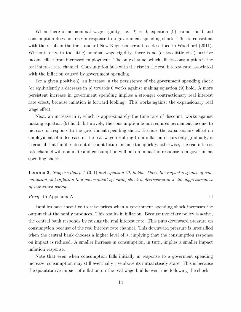
When there is no nominal wage rigidity, i.e. ξ = 0, equation (9) cannot hold and

consumption does not rise in response to a government spending shock. This is consistent

with the result in the the standard New Keynesian result, as described in Woodford (2011).

Without (or with too little) nominal wage rigidity, there is no (or too little of a) positive

income effect from increased employment. The only channel which affects consumption is the

real interest rate channel. Consumption falls with the rise in the real interest rate associated

with the inflation caused by government spending.

For a given positive ξ, an increase in the persistence of the government spending shock

(or equivalently a decrease in %) towards 0 works against making equation (9) hold. A more

persistent increase in government spending implies a stronger contractionary real interest

rate effect, because inflation is forward looking. This works against the expansionary real

wage effect.

Next, an increase in r, which is approximately the time rate of discount, works against

making equation (9) hold. Intuitively, the consumption boom requires permanent income to

increase in response to the government spending shock. Because the expansionary effect on

employment of a decrease in the real wage resulting from inflation occurs only gradually, it

is crucial that families do not discount future income too quickly; otherwise, the real interest

rate channel will dominate and consumption will fall on impact in response to a government

spending shock.

Lemma 3. Suppose that ρ ∈ (0, 1) and equation (9) holds. Then, the impact response of con-

sumption and inflation to a government spending shock is decreasing in λ, the aggressiveness

of monetary policy.

Proof. In Appendix A.

Families have incentive to raise prices when a government spending shock increases the

output that the family produces. This results in inflation. Because monetary policy is active,

the central bank responds by raising the real interest rate. This puts downward pressure on

consumption because of the real interest rate channel. This downward pressure is intensified

when the central bank chooses a higher level of λ, implying that the consumption response

on impact is reduced. A smaller increase in consumption, in turn, implies a smaller impact

inflation response.

Note that even when consumption falls initially in response to a goverment spending

increase, consumption may still eventually rise above its initial steady state. This is because

the quantitative impact of inflation on the real wage builds over time following the shock.

14

While inflation and the real interest rate channel may drive down consumption initially,

as the inflation drives up the nominal price level, this will eventually put downward pressure

on real marginal cost. Eventually, the stimulative effect of the real wage channel may more

than offset the real interest rate channel leading, to an increase in consumption.

Lemma 4. Let ρ ∈ (0, 1). Suppose β > 0.5. The impact response of inflation to a govern-

ment spending shock is increasing in ρ if ρ < 1 − (κ[s(1/α−1)λ−ξ]β

)12 , and is decreasing in ρ if

the inequality is reversed.

Proof. In Appendix A.

The response of inflation on impact exhibits a hump-shaped pattern with ρ. Two forces

affect current inflation: the negative wealth effect and the combined effects generated by

expected inflation which includes the real interest rate channel and the real wage channel.

When ρ increases, the negative wealth effect becomes larger putting downward pressure

on current inflation, while the positive combined effects generated by expected inflation

become larger putting upward pressure on current inflation. So the overall response of

inflation could be greater or smaller depending on the relative size of these two forces.

Initially, the combined effects increase faster, so the inflation response becomes greater.

Yet, when ρ increases further, the real interest rate becomes higher, which weakens the

combined effects. Moreover, the effect from the real wage channel becomes weaker because

the nominal wage increases with higher inflation. Consequently, the overall response of

current inflation would be smaller if ρ becomes large enough.

In addition, when λ decreases, the real interest rate channel is dampened. The peak

occurs at a larger ρ. When ξ increases, the real wage channel is intensified. There is also a

rightward shift of the peak. If λ approaches its lower bound (or equivalently, ξ approaches

its upper bound), i.e. λ = αξs(1−α)

, we obtain a limiting case where the hump disappears and

the size of inflation increases in ρ.

Next, we are interested in not simply the consumption multiplier on impact, but also

the accumulated change in consumption for a given accumulated change in government

spending.7 We define the cumulative discounted consumption multiplier, or simply the

cumulative multiplier, as the following

µcumc =s

1− s

[∑∞t=0 β

t (dct/dg0)∑∞t=0 β

t (dgt/dg0)

]7This cumulative approach for defining the multiplier is advocated, for example, by Drautzburg and Uhlig

(2015) and Ramey and Zubairy (2016).

15

The s/ (1− s) multiplicand appears because we want µcumc to be a derivative (unit change

given a unit change) as opposed to an elasticity (percentage change given a percentage

change). Because gt is first-order autoregressive, we have∑∞

t=0 βt (dgt/dg0) = 1/ (1− ρβ).

The final term,∑∞

t=0 βt (dct/dg0), is the accumulated consumption response. Given the

formula from Theorem 2, we have

∞∑t=0

βt (dct/dg0) =∞∑t=0

βt

(d[χgt + ξ [s (1/α− 1)]−1 pt−1

]dg0

)

=χ

1− ρβ+

αξ

s (1− α)

∞∑t=0

βt

(t−1∑s=0

dπsdg0

)=

χ

1− ρβ+

αξγβ

s (1− α) (1− β) (1− ρβ)

Combining terms, the cumulative multiplier is

µcumc =s

1− s

[χ+

αξγβ

s (1− α) (1− β)

]

Next, we plug specific parameters into the model and study the equilibrium response

coefficients. For each parameterization reported, the equilibrium is locally unique. Most of

the parameters are held fixed. The discount factor, β, is set equal to 0.99. The elasticity

of output with respect to labor, α, is set to 2/3. The share of consumption in GDP, s, is

assumed to be 0.8 so that the share of government spending is 0.2. The probability that a

family producer cannot reset its good price, θ, is set to equal 0.75 so that the average price

duration is one year. Then we have that κ = (1−θ)(1−βθ)θ

= 0.0858. We set the weight in the

nominal wage, ξ, to 0.156 so that the (quarterly) frequency of wage change, (1− ξ) (1− θ),is equal to 0.211 as in Barattieri et al. (2014). Figure 2 plots consumption and inflation

responses for particular equilibria as we, in turn, vary ρ and λ.

Panel (a) of the figure presents the elasticity of inflation on impact to a government

spending shock for alternative values of ρ. The inflation multiplier on impact is in the range

of 0.009 and 0.05 and is increasing in ρ. Intuitively, a more persistent government spending

shock implies that output will be above the steady state for a longer period of time, and

forward-looking price setters will recognize this and initiate larger initial price increases right

away.

Panel (b) plots the consumption multiplier on impact for alternative value of ρ. Over this

16

Figure 2: Response of economy to a government spending shock, varying ρ and λ

0 0.2 0.4 0.6 0.8 1

;

0

0.02

0.04

0.06(a) impact inflation elasticity

0 0.2 0.4 0.6 0.8 1

;

-0.02

0

0.02

0.04

(b) impact consumption multiplier

0 0.2 0.4 0.6 0.8 1

;

0

5

10(c) cum. consumption multiplier

0.3 0.4 0.5 0.6 0.7

6

0.04

0.06

0.08(d) impact inflation elasticity

0.3 0.4 0.5 0.6 0.7

6

-0.4

-0.2

0

0.2(e) impact consumption multiplier

0.3 0.4 0.5 0.6 0.7

6

5

10

15(f) cum. consumption multiplier

Notes: ρ = persistence of the government spending shock; λ = responsiveness of interest rate to

inflation.

17

range of ρ, the consumption multiplier is initially increasing, and then turns decreasing, as

ρ becomes larger. This is consistent with Lemma 2. As government spending becomes more

persistent, there is a larger inflation response. This implies a larger reduction in the real

wage both today and in the future which increases the families’ returns to production. Panel

(c) plots the cumulative consumption multiplier, where we discount future values of both

consumption and government spending responses by β. As with the impact consumption

multiplier, the cumulative consumption multiplier is increasing over this range of ρ.

The analogous information is plotted in panels (d) through (f), except we have λ varying

instead of ρ. These panels demonstrate the interaction between monetary and fiscal policy

in our model. As λ increases, all three responses become smaller. For panel (d), the inflation

response is decreasing because the central bank is more aggressively combating inflation.

As the central bank responds more aggressively, it is raising the real interest rate by a

larger amount. This amplifies the contractionary intertemporal substitution effect as families

reduce consumption when facing a higher real interest rate.

4 Calvo-type Sticky Wages

With the above formulation of nominal wage rigidity, any shock that has a permanent effect

on the price level will have a permanent effect on output. For example, suppose there is

a transitory, positive shock to government spending. Under the conditions of Lemma 1,

this drives up the price level. Although inflation might converge back to the steady state

following the shock, the long-run price level would be higher. In turn, the long run real wage

would be lower, which would be associated with higher long-run output.

Next, we study an alternative model to undo the permanent real effects of transitory

government spending shocks. Specifically, we assume that nominal wages are set in Calvo-

type staggered contracts analogous to the price contracts described in Section 2.1. Moving

to Calvo-style wage setting demonstrates that the mechanism can work in a more traditional

macro model; however, we will lose analytic tractability and instead rely on simulation

methods to establish the real wage channel for fiscal multipliers.

The utility function of family v is

U (v) =∞∑t=0

βtE0

[log [Ct (v)] + ζn log [1−N s

t (v)] + ζm log

[Mt (v)

Pt

]]

where N st (v) denotes hours worked and the family’s time endowment is normalized to 1.

18

The budget constraint is

Mt (v) +Bt(v)

Rt

= Bt−1(v) +Mt−1 (v) + Πt(v) + (1 + τw)Wt (v)N st (v)− PtCt (v)−Ht(v)

which is the same as the budget constraint in Section 2.1 except that labor income is now

subsidized at a rate of τw. In each period, families cannot renegotiate their wage contracts

with probability θw ∈ [0, 1]. Each family sets its wage rate, Wt(v), subject to the following

downward-sloping labor demand constraint:

Nt+i|t (v) =

[Wt (v)

Wt+i

]−εwNdt+i

where Wt ≡ [∫ 1

0Wt(v)1−εwdv]

11−εw is the nominal wage aggregator, εw is the elasticity of

substitution between types of labor, and Ndt is total labor demand. τw is chosen to eliminate

the distortion from monopolistic competition in labor markets. Let wt = Wt

Ptdenote the real

wage. The Phillips curve previously represented by equation (1) becomes

πt = κ [(1/α− 1) yt + wt] + βEt (πt+1)

Let πw,t = Wt

Wt−1denote the wage inflation rate. Then the change in the real wage is the

difference between wage inflation and price inflation

wt = wt−1 + πw,t − πt

Let variables with bars denote steady-state values. In the steady state, labor supply is

identical across families, i.e., N = N (v). Let µn ≡ N/(1− N). The wage Phillips curve is

πw,t = κw [(µn/α) yt + ct − wt] + βEt (πw,t+1)

where κw = (1−θw)(1−βθw)θw(1+µnεw)

.

We then simulate the model. This requires us to choose specific parameter values. We

set β, α, and s equal to their values from the previous section. ζn is set to 5/3 so that family

members spend 1/3 of their time working in the steady state, i.e. N = 1/3. εw is set to 21

so that the gross markup in labor markets, εw/(εw− 1), is equal to 1.05, consistent with the

findings of Christiano et al. (2005). Recall that θ measures the degree of price rigidity and

θw measures that of nominal wage rigidity. We set θ = 0.65 and θw = 0.73, which are the

19

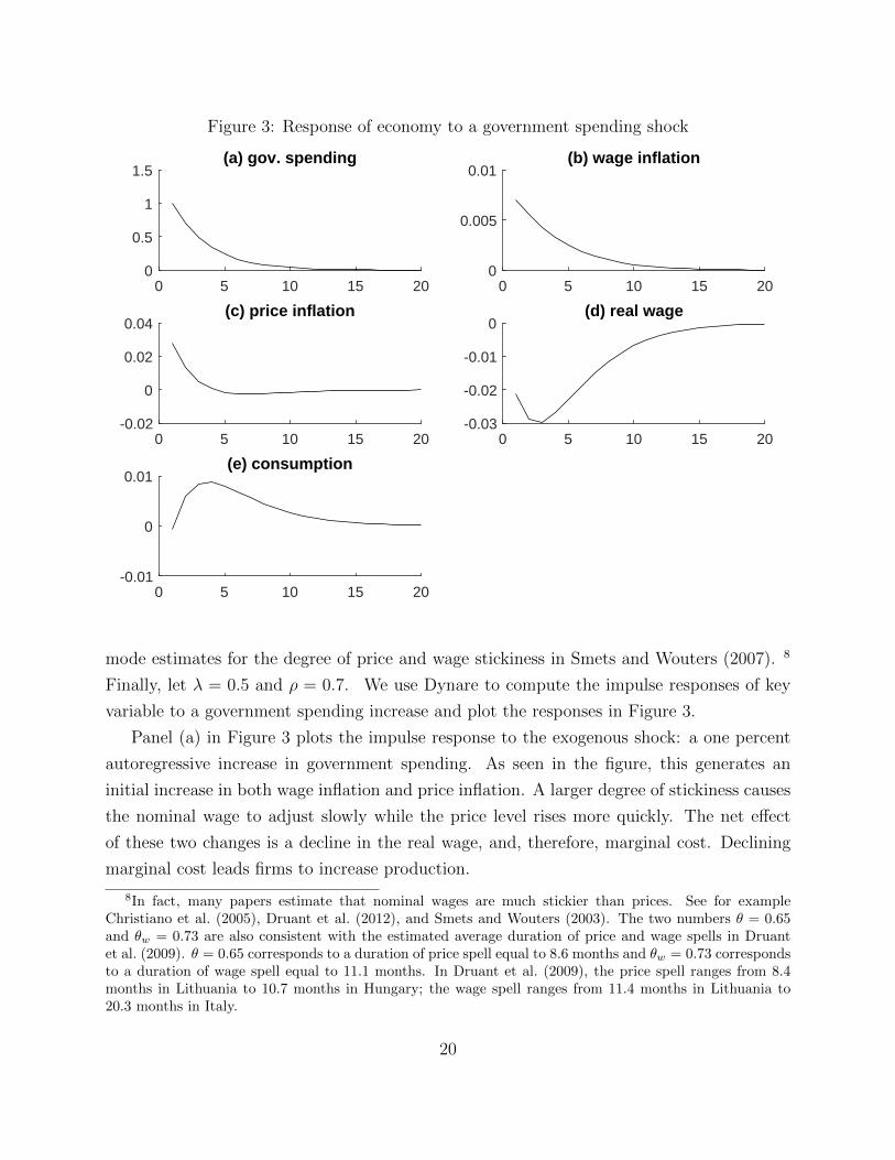
Figure 3: Response of economy to a government spending shock

0 5 10 15 200

0.5

1

1.5(a) gov. spending

0 5 10 15 200

0.005

0.01(b) wage inflation

0 5 10 15 20-0.02

0

0.02

0.04(c) price inflation

0 5 10 15 20-0.03

-0.02

-0.01

0(d) real wage

0 5 10 15 20-0.01

0

0.01(e) consumption

mode estimates for the degree of price and wage stickiness in Smets and Wouters (2007). 8

Finally, let λ = 0.5 and ρ = 0.7. We use Dynare to compute the impulse responses of key

variable to a government spending increase and plot the responses in Figure 3.

Panel (a) in Figure 3 plots the impulse response to the exogenous shock: a one percent

autoregressive increase in government spending. As seen in the figure, this generates an

initial increase in both wage inflation and price inflation. A larger degree of stickiness causes

the nominal wage to adjust slowly while the price level rises more quickly. The net effect

of these two changes is a decline in the real wage, and, therefore, marginal cost. Declining

marginal cost leads firms to increase production.

8In fact, many papers estimate that nominal wages are much stickier than prices. See for exampleChristiano et al. (2005), Druant et al. (2012), and Smets and Wouters (2003). The two numbers θ = 0.65and θw = 0.73 are also consistent with the estimated average duration of price and wage spells in Druantet al. (2009). θ = 0.65 corresponds to a duration of price spell equal to 8.6 months and θw = 0.73 correspondsto a duration of wage spell equal to 11.1 months. In Druant et al. (2009), the price spell ranges from 8.4months in Lithuania to 10.7 months in Hungary; the wage spell ranges from 11.4 months in Lithuania to20.3 months in Italy.

20

Increased production puts more income into the hands of families, which allows them

to pay the tax bill associated with the increased government spending and also buy more

consumption goods. In absence of the falling real wage, consumption would instead fall.

This is because, ceteris paribus, the active monetary policy implies that increased inflation

would drive up the real interest rate, leading families to reduce current consumption and

increase savings.

Eventually, government spending asymptotes to its steady state. This causes price infla-

tion to return to zero, which means that the price level converges to a new long run steady

state. The nominal wage converges as well although this variable moves to its new steady

state more slowly. Note that both the nominal wage and the price level converge in per-

centage deviation terms by the same amount. This implies that the long run real wage is

identical to its pre-shock level. With the real wage having converged and the real interest

rate having converged (because inflation returned to zero), consumption returns to its initial

steady state.

To explore the importance of the sticky wage assumption, we change the specification

by decreasing the degree of nominal wage rigidity. In the benchmark parameter, θw equals

0.73, whereas, we set θw = 0.65 to demonstrate the effect of less sticky nominal wages. The

other parameters are unchanged.

The solid lines in Figure 4 are the impulse responses from our benchmark case. The

dashed red lines represent an alternative case in which price and the nominal wage have the

same degree of stickiness (θ = θw = 0.65). As seen in the figure, consumption falls on impact

and remains below zero for several periods in the alternative case. Price inflation increases

with less sticky nominal wages which causes the nominal price level to increase initially.

This effect tends to push down the real wage; however, because we decrease θw relative to

the benchmark case, the nominal wage moves up towards its new steady state much more

quickly. This is implied by panel (b) where wage inflation is much larger.

This means that the real wage decrease is much more muted with less sticky nominal

wages. Its expansionary effect is insufficiently large to overcome the contractionary effect of

the real interest rate increase caused by inflation paired with an active interest rate rule.

Next, we consider the effect of changing the aggressiveness of monetary policy with respect

to inflation, λ. The solid lines in Figure 5 reflect the benchmark case. The dashed red lines

reflect the case where policy is much more active, with λ = 1.5. In this case, the increase

in inflation caused by government spending induces a very large increase in the nominal

interest rate, and therefore the real interest rate. With a large interest rate increase, the

21

Figure 4: Response of economy to a government spending shock, varying the degree of wagerigidity

0 5 10 15 200

0.5

1

1.5(a) gov. spending

0 5 10 15 200

0.005

0.01

0.015(b) wage inflation

0 5 10 15 20-0.02

0

0.02

0.04(c) price inflation

0 5 10 15 20-0.03

-0.02

-0.01

0(d) real wage

0 5 10 15 20-0.01

0

0.01(e) consumption

w = 0.73

w = 0.65

Notes: θw = 0.73 reflects the benchmark case; θw = 0.65 reflects less sticky nominal wages.

22

Figure 5: Response of economy to a government spending shock, varying the responsivenessof the interest rate rule

0 5 10 15 200

0.5

1

1.5(a) gov. spending

0 5 10 15 200

0.005

0.01(b) wage inflation

0 5 10 15 20-0.02

0

0.02

0.04(c) price inflation

0 5 10 15 20-0.04

-0.02

0(d) real wage

0 5 10 15 20-0.02

0

0.02(e) consumption

= 0.5

= 1.5

Notes: λ = 0.5 reflects the benchmark case; λ = 1.5 reflects relatively active policy.

23

standard real interest rate effect leads families to dramatically reduce consumption. The real

interest rate channel initially dominates our new real wage channel. However, eventually, as

the inflation rate begins to return to its steady state, the real interest rate also begins to

return to its steady state.

At this point, our new proposed effect dominates as the resulting higher price level

combined with a stickier nominal wage drives down the real wage. Examining panel (e), by

horizon two, consumption is above the steady state. After this, it slowly converges back to

its steady state as the nominal wage “catches up” with the increase in the price level.

5 Discussion

5.1 Existing Research: Sticky Wages as an Element for Generat-

ing Large Multipliers

We have shown that sticky wages and prices are sufficient to generate a positive consump-

tion multiplier and hence an output multiplier that is larger than one. Another paper that

succeeds in producing a positive consumption multiplier is Rendahl (2016). The author uses

an inertial labor market to achieve this goal: government spending reduces unemployment,

which is persistent into the future; a brighter future increases current consumption, under

the condition that the elasticity of intertemporal substitution is low. This mechanism works

only when unemployment exists, meaning that the efficacy of monetary policy is constrained.

In normal times (outside the liquidity trap), full employment is ensured, hence an increase in

government spending cannot increase employment further. Therefore, it cannot increase cur-

rent consumption in normal times. Our model, instead, can generate a positive consumption

multiplier without the zero lower bound.

There are also models with rule-of-thumb consumers that emphasize the role of sticky

wages in facilitating realistic responses of macroeconomic variables to a government spending

shock. Colciago (2011) shows that nominal wage rigidity influences both the response of

consumption to a government spending shock and the conditions for equilibrium determinacy.

Furlanetto (2011) finds that adding nominal wage rigidity to the Galı et al. (2007) model

improves the model’s performance in matching real wage dynamics. The main difference

between our model and theirs is that we do not rely on the use of rule-of-thumb consumers

to generate a positive consumption multiplier.

There are other papers that are more tangentially related to our work. These papers

24

also illustrate the transmission from higher prices to lower real wages and then to higher

employment, resulting from sticky nominal wages. For example, Schmitt-Grohe and Uribe

(2017) build a model in which a negative confidence shock induces a recession and a liquidity

trap. Output growth is gradually restored. However, because of downward nominal wage

rigidity, real wages fail to fall to levels required by the recovery of full employment. There-

fore, a jobless growth recovery occurs.9 Again, the zero lower bound on nominal interest

rates, in addition to downward nominal wage rigidity, is required for the model to generate

large contractions with jobless recoveries. Bordo et al. (2000) emphasize the importance of

sticky wages in propagating negative monetary shocks during the Great Depression. The

mechanism illustrated in their model is that a monetary innovation causes the price level

to increase, while nominal wages respond gradually. The persistent decline in the real wage

induces an increase in labor hours and output. While a positive money growth innovation

under sticky wages is able to generate a large output increase, fiscal policy analysis is left

untouched in Bordo et al. (2000).

5.2 Comparing the Sticky Wage Channel to Other Approaches

Various mechanisms have been offered to explain how, within an optimizing, dynamic equi-

librium model, increases in government spending might stimulate private economic activity.

We view our mechanism as an important contribution because it involves a very minor de-

parture, the empirically relevant sticky wage assumption, from the canonical New Keynesian

model.

First, as discussed in the introduction, several papers, such as Christiano (2004), Chris-

tiano et al. (2011), Eggertsson and Woodford (2006), Mertens and Ravn (2014) and Woodford

(2011), have shown that under a particular class of monetary policies, the output multiplier

can be greater than one in a New Keynesian model. This occurs when the central bank

raises the interest rate in a less than one-for-one manner with inflation, which might arise

if, for example, the policy rate were stuck at the zero lower bound. While this mechanism

works, it requires monetary policy to be passive.

Second, a number of authors, including Bouakez and Rebei (2007), demonstrate that

when private and public consumption are Edgeworth complements for households, an in-

crease in government spending can increase private consumption. Intuitively, this arises

because government purchases increase the marginal utility of private consumption. The

9In Schmitt-Grohe and Uribe (2016), the authors investigate optimal government policies needed toeliminate the negative externality caused by downward nominal wage rigidity.

25

government purchases therefore act as a preference shock, so that households will increase

consumption even if the real interest rate and real wage were unchanged.

While it is possible to posit examples of complementarity between public and private

goods, e.g. better highways may increase vacations taken and therefore vacation spending, it

seems just as easy to find examples of substitutability. For example, the provision of primary

and secondary education by the government is likely a substitute for private provision of those

services. At a more fundamental level, by coupling a preference effect with the deadweight

loss of taxation, this approach is very close to simply assuming the result.

Closely related to the private-public consumption complementarity approach to generat-

ing large multipliers is to assume that labor and private consumption are complements in the

utility function. This mechanism is discussed, for example, in Hall (2009). According to this

channel, the deadweight loss of government spending increases labor supply. An increase in

labor supply in turn increases the marginal utility of private consumption. Households will

then increase consumption, resulting in an output multiplier that is greater than one.

Whether labor and consumption are complements in production is an empirical question.

It is worth noting, however, that a government’s justification for public spending as stimulus

to its citizenry might not be compelling. It would go something like this: “By purchasing

public goods and making you poorer through taxes, you will work harder which will increase

your hunger. Greater hunger will in turn boost consumption spending.”

Finally, several existing explanations for a large multiplier can broadly fall under an um-

brella of winner/loser mechanisms. These include, for example, Eggertsson and Krugman

(2012) and Galı et al. (2007). In each case, aggregate consumption increases because the

increased consumption of one group of agents outweighs the decreased consumption experi-

enced by another group of agents. In the above examples, the winners are either borrowing

constrained or consume in a rule-of-thumb manner. In each example, the losers behave as

permanent income consumer.

In contrast to the above three channels for generating large fiscal multipliers, our ap-

proach does not depend upon: a particular stance of monetary policy, non-separability in

preferences, or one group of agents suffering at the expense of the other group.

6 Conclusion

One hallmark of the Keynesian approach to business cycle stabilization is that wages do not

clear the labor market, leading to a shortage of labor demand relative to people’s willingness

26

to work at the going wage. As discussed in the introduction, there is ample evidence in favor

of a high nominal wage rigidity. Since firms care about the real, as opposed to nominal,

wage when making labor decisions, the nominal price level provides an indirect channel by

which the government can close the gap between labor supply and demand when wages are

too high. In a model where government spending puts an upward pressure on goods prices,

this spending will also drive down the real wage when nominal wages are fixed, leading to

an employment boom capable of increasing consumption as well as financing the additional

tax bill.

Appendix A Proofs of Theorems and Lemmas

A.1 Proof of Theorem 1

Proof. The second-order difference equation in πt is given by

βEt (πt+2)− [1 + β + κξ − sκ (1/α− 1)λ]Et (πt+1) + πt = κ (1− s) (1/α− 1) (1− ρ) gt

The two roots of the characteristic equation are

e1 =Φ +

√Φ2 − 4β

2β

and

e2 =Φ−

√Φ2 − 4β

2β

where Φ = 1 + β + κξ − sκ (1/α− 1)λ. We have the following two cases to consider.

Case (i):

κξ − sκ (1/α− 1)λ < 0 ⇐⇒ λ >αξ

s(1− α)

If Φ−2β > 0 ⇐⇒ λ < α(1−β+κξ)sκ(1−α)

, then the smaller root e2 >[1+β+κξ−sκ(1/α−1)λ]−

√[1−β+κξ−sκ(1/α−1)λ]2

2β=

1. Hence both roots are outside the unit circle and the equilibrium is locally unique.

If Φ − 2β < 0 ⇐⇒ λ > α(1−β+κξ)sκ(1−α)

, then the larger root −1 < e1 < 1 and hence the

equilibrium is indeterminate.

Case (ii):

κξ − sκ (1/α− 1)λ > 0 ⇐⇒ λ <αξ

s(1− α)

27

The two roots are

e1 = 1 +Φ− 2β +

√Φ2 − 4β

2β

= 1 +Φ− 2β +

√(1− β)2 + 2(1 + β)[κξ − sκ (1/α− 1)λ] + [κξ − sκ (1/α− 1)λ]2

2β

and

e2 = 1 +Φ− 2β −

√Φ2 − 4β

2β

= 1 +Φ− 2β −

√(1− β)2 + 2(1 + β)[κξ − sκ (1/α− 1)λ] + [κξ − sκ (1/α− 1)λ]2

2β

Since

[1− β + κξ − sκ (1/α− 1)λ]2 = (1− β)2 + 2(1− β)[κξ − sκ (1/α− 1)λ] + [κξ − sκ (1/α− 1)λ]2

< (1− β)2 + 2(1 + β)[κξ − sκ (1/α− 1)λ] + [κξ − sκ (1/α− 1)λ]2

we have that e1 > 1 and −1 < e2 < 1. Hence the equilibrium is not unique in case (ii).

Overall, λ should satisfy αξs(1−α)

< λ < α(1−β+κξ)sκ(1−α)

so that the equilibrium is locally unique.

A.2 Proof of Theorem 2

Proof. First, substitute out yt from (2) into (1) and get

πt = κ(1/α− 1) [sct + (1− s)gt]− ξpt+ βEtπt+1 (10)

Update t to t+ 1 and take expectation.

Etπt+1 = κ(1/α− 1) [sEtct+1 + (1− s)Etgt+1]− ξEtpt+1+ βEtπt+2 (11)

Subtract (10) from (11) and then use (3) to return a second-order difference equation in πt.

βEt (πt+2)− [1 + β + κξ − sκ (1/α− 1)λ]Et (πt+1) + πt = κ (1− s) (1/α− 1) (1− ρ) gt

Next, guess a solution that takes the form πt = γgt and plug that guess into the above

28

equation.

ρ2βγgt − ρ (1 + β + κξ − sκ (1/α− 1)λ) γgt + γgt = κ (1− s) (1/α− 1) (1− ρ) gt

Then, the solution for the undetermined coefficient γ is

γ =κ (1/α− 1) (1− s) (1− ρ)

1 + βρ2 + [sκ (1/α− 1)λ− (1 + κξ + β)]ρ

Using the solution for inflation as a function of government purchases, we can rewrite the

inflation Euler equation as

(1− ρβ) γgt + κξγgt + κξpt−1 = sκ (1/α− 1) ct + κ (1/α− 1) (1− s) gt

Next, we rearrange this expression to have

ct =[1 + κξ − ρβ] γ − κ (1/α− 1) (1− s)

sκ (1/α− 1)gt +

αξ

(1− α)spt−1

A.3 Proof of Lemma 1

Proof. From equation (7) and our assumption that ρ < 1, γ > 0 if and only if

1 + βρ2 > ρ [1 + β + κξ − sκλ (1/α− 1)]

Rearranging this expression,

κ−1ρ−1 (1− ρ) (1− βρ) > ξ − sλ (1/α− 1) (12)

The term on the left-hand side of (12) is positive given our restrictions on ρ, κ and β. The

term on the right-hand side is negative because of our restriction that guarantees local

uniqueness.

29

A.4 Proof of Lemma 2

Proof. According to equation (8), χ > 0 if and only if

1− ρ1− ρ+ sκ(1/α−1)λρ−κξ

1−βρ+κξ

> 1

Recall that local uniqueness requires

αξ

s (1− α)< λ <

α (1− β + κξ)

sκ (1− α)

Given that λ > αξs(1−α)

, we have

1− ρ+sκ (1/α− 1)λρ− κξ

1− βρ+ κξ> 1− ρ+

κξρ− κξ1− βρ+ κξ

=(1− ρ)(1− βρ)

1− βρ+ κξ> 0.

Using % ≡ 1ρ− 1 and r ≡ 1− β, we can rewrite (9) as ρ < κξ

1−β+κξ. If ρ < κξ

1−β+κξ, then

λ <α (1− β + κξ)

sκ (1− α)<

αξ

s (1− α) ρ

Having λ < αξs(1−α)ρ

, we obtain

sκ (1/α− 1)λρ− κξ < 0

Hence1− ρ

1− ρ+ sκ(1/α−1)λρ−κξ1−βρ+κξ

> 1

A.5 Proof of Lemma 3

Proof. Recall that γ is

γ =κ (1/α− 1) (1− s) (1− ρ)

1 + βρ2 + [sκ (1/α− 1)λ− (1 + κξ + β)]ρ(13)

30

Because ρ < 1, γ is positive. An increase in λ increases the denominator on the right-hand

side of (13) and therefore decreases γ. Next, χ > 0. It is given by

χ =(1 + κξ − ρβ) γ − κ (1/α− 1) (1− s)

sκ (1/α− 1)

Thus, a decrease in γ resulting from an increase in λ reduces χ.

A.6 Proof of Lemma 4

Proof. Recall that γ is

γ =κ (1/α− 1) (1− s) (1− ρ)

1 + βρ2 + ρ [sκ (1/α− 1)λ− (1 + κξ + β)]

Then, we have

∂γ

∂ρ=−κ (1/α− 1) (1− s)[−β(1− ρ)2 − κξ + sκ (1/α− 1)λ]

42

where 4 = 1 + βρ2 + ρ [sκ (1/α− 1)λ− (1 + κξ + β)].

The root of the equation −β(1− ρ)2− κξ+ sκ (1/α− 1)λ = 0 is 1− (κ[s(1/α−1)λ−ξ]β

)12 . Given

the restriction imposed on λ that ensures a locally unique equilibrium, we can show that

as long as β > 0.5, 1 − (κ[s(1/α−1)λ−ξ]β

)12 ∈ (0, 1). Thus, if ρ < 1 − (κ[s(1/α−1)λ−ξ]

β)12 , we have

∂γ∂ρ> 0. And if ρ > 1− (κ[s(1/α−1)λ−ξ]

β)12 , ∂γ

∂ρ< 0.

Appendix B Intuition for Lemma 4

The starting point is:

Et (πt+2) + β−1 (κ [sλ (1− α)− ξ]− 1− β)Et (πt+1) + β−1πt = −κ (1− s) (1− α)Et (∆gt+1)

Using lag operator notation:

[1 + β−1 (κ [sλ (1− α)− ξ]− 1− β)L+ β−1L2

]Et (πt+2) = −κ (1− s) (1− α)Et (∆gt+1)

Note that the appearence of ξ only works to make the monetary policy less “active”. Other

than this, it does not influence the dynamics of inflation. Therefore, define λ = sλ (1− α)−ξ.

31

. [1 + β−1

(κλ− 1− β

)L+ β−1L2

]Et (πt+2) = −κ (1− s) (1− α)Et (∆gt+1)

Next, factoring the lag polynomial gives us:

(1− Λ1L) (1− Λ2L)Et (πt+2) = −κ (1− s) (1− α)Et (∆gt+1)

It is possible to prove both roots are unstable, therefore we solve them forward.

(−Λ1L) (−Λ1L)−1 (−Λ2L) (−Λ2L)−1 (1− Λ1L) (1− Λ2L)Et (πt+2) = −κ (1− s) (1− α)Et (∆gt+1)

(Λ1L) (Λ2L)[1− (Λ1L)−1] [1− (Λ2L)−1]Et (πt+2) = −κ (1− s) (1− α)Et (∆gt+1)

Rearranging,

πt =−κ (1− s) (1− α)

Λ1Λ2

[1− (Λ1L)−1]Et ∆gt+1 + (Λ2)−1 ∆gt+2 + (Λ2)−2 ∆gt+3 + ...

Taking this out even further,

πt =−κ (1− s) (1− α)

Λ1Λ2

Et

∆gt+1 + (Λ2)−1 ∆gt+2 + (Λ2)−2 ∆gt+3 + ...

(Λ1)−1 [∆gt+2 + (Λ2)−1 ∆gt+3 + (Λ2)−2 ∆gt+4 + ...]

+ ...

(Λ2)−1 [∆gt+3 + (Λ2)−1 ∆gt+4 + (Λ2)−2 ∆gt+5 + ...]

+ ...

Simplyifying further

πt =−κ (1− s) (1− α) (ρ− 1)

Λ1Λ2

1 + ρ (Λ2)−1 + ρ2 (Λ2)−2 + ...

(Λ1)−1 [ρ+ (Λ2)−1 ρ2 + (Λ2)−2 ρ3 + ...]

+ ...

(Λ2)−1 [ρ2 + (Λ2)−1 ρ3 + (Λ2)−2 ρ4 + ...]

+ ...gt

Doing it again,

πt =−κ (1− s) (1− α) (ρ− 1)

Λ1Λ2

1 + ρ (Λ2)−1 + ρ2 (Λ2)−2 + ...

(Λ1)−1 [ρ+ (Λ2)−1 ρ2 + (Λ2)−2 ρ3 + ...]

+ ...

(Λ1)−2 [ρ2 + (Λ2)−1 ρ3 + (Λ2)−2 ρ4 + ...]

+ ...gt

32

Getting there,

πt =−κ (1− s) (1− α) (ρ− 1)

Λ1Λ2

1

1− (ρ/Λ2)+

(ρ

Λ1

)(1

1− (ρ/Λ2)

)+

(ρ

Λ1

)2(1

1− (ρ/Λ2)

)+ ...

gt

πt =−κ (1− s) (1− α) (ρ− 1)

Λ1Λ2

1

[1− (ρ/Λ2)] [1− (ρ/Λ1)]

gt

πt = −κ (1− s) (1− α) (ρ− 1)

1

[Λ1 − ρ] [Λ2 − ρ]

gt

Appendix C Lemma 5

Lemma 5. Let ρ ∈ (0, 1). Let ρ denote the smaller root of the equation βsκ (1/α− 1)λρ2−2βκξρ + κξ(1 + κξ + β) − (1 + κξ)sκ (1/α− 1)λ. If the parameter set is configured such

that ρ > 0 (i.e. λ < (1+κξ+β)αξ(1+κξ)s(1−α)

), then the impact response of consumption to a government

spending shock is increasing in ρ if ρ < ρ, and it is decreasing in ρ if the inequality is

reversed.

Proof. The partial derivative of χ with respect to ρ is given by

∂χ

∂ρ=

1− ss

[βsκ (1/α− 1)λρ2 − 2βκξρ+ κξ(1 + κξ + β)− (1 + κξ)sκ (1/α− 1)λ

Ω2(1− βρ+ κξ)2(1− ρ)2]

where Ω = 1 + sκ(1/α−1)λρ−κξ(1−βρ+κξ)(1−ρ)

.

Let ρ and ρ denote the two roots of the equation βsκ (1/α− 1)λρ2 − 2βκξρ + κξ(1 + κξ +

β)− (1 +κξ)sκ (1/α− 1)λ = 0. Hence, if ρ < ρ or ρ > ρ, we have ∂χ∂ρ> 0. And if ρ < ρ < ρ,

∂χ∂ρ< 0.

We can show that ρ < 1. Moreover, ρ > 1 because of our restriction that guarantees a

unique equilibrium.

If λ < (1+κξ+β)αξ(1+κξ)s(1−α)

, then ρ > 0. Therefore, ∂χ∂ρ> 0 when ρ < ρ, and ∂χ

∂ρ< 0 when ρ > ρ.

Establishing an intuition for Lemma 5 is challenging. If λ > (1+κξ+β)αξ(1+κξ)s(1−α)

, then ρ < 0.

The real interest rate channel with an active monetary policy is strong enough so that the

size of the response of consumption on impact decreases in ρ ∈ (0, 1). Lemma 5 focuses on

the case where the impact response of consumption exhibits a hump-shaped pattern. This

pattern also results from the interactions among the negative wealth effect, the real interest

rate channel and the real wage channel, as explained in Lemma 4. One thing to add is that

33

as long as β > 0.2, the peak of the consumption response occurs at a smaller ρ than that of

the inflation response does, i.e. ρ < 1− (κ[s(1/α−1)λ−ξ]β

)12 .

Mathematically, ∂χ∂ρ

can be written as

∂χ

∂ρ=α(1 + κξ − βρ)

κs(1− α)

∂γ

∂ρ− αβγ

κs(1− α)

The first term is the influence from current inflation and it governs the effects of the

real wage channel. This term varies with ∂γ∂ρ

, the change in the response of contemporaneous

inflation with respect to the persistency of the government spending shock. The second term

is related to the size of the increase in the real interest rate because it reflects the response

of expected inflation. A higher expected inflation caused by a more persistent government

spending shock would result in a larger real interest rate provided that the monetary policy

is active. Consequently, a larger real interest rate prevents private consumption from increas-

ing. Because the negative sign of the second term, the peak of the consumption response

occurs earlier than that of the inflation response.

34

References

Akerlof, G. A., Dickens, W. T., Perry, G. L., Gordon, R. J., and Mankiw, N. G. (1996), “The

Macroeconomics of Low Inflation,” Brookings Papers on Economic Activity, 1996(1), 1-76.

Altonji, J. G. and Devereux, P. J. (2000), “The Extent and Consequences of Downward

Nominal Wage Rigidity,” in Research in Labor Economics, 383-431.

Auerbach, A. and Gorodnichenko, Y. (2012), “Measuring the Output Responses to Fiscal

Policy,” American Economic Journal: Macroeconomics, 4, 1-27.

Avouyi-Dovi, S., Fougere, D., and Gautier, E. (2013), “Wage Rigidity, Collective Bargaining,

and the Minimum Wage: Evidence from French Agreement Data,” Review of Economics

and Statistics, 95(4), 1337-1351.

Barattieri, A., Basu, S., and Gottschalk, P. (2014), “Some Evidence on the Importance of

Sticky Wages,” American Economic Journal: Macroeconomics, 6(1), 70-101.

Barro, R. and Grossman, H. (1971), “A General Disequilibrium Model of Income and Em-

ployment,” American Economic Review, 61, 82-93.

Bewley, T. F. (1998), “Why Not Cut Pay?” European Economic Review, 42(3), 459-490.

Bihan, H. L., Montornes, J., and Heckel, T. (2012), “Sticky Wages: Evidence from Quarterly

Microeconomic Data,” American Economic Journal: Macroeconomics, 4(3), 1-32.

Bernanke, B. and Woodford, M. (1997) “Inflation Forecasts and Monetary Policy,” Journal

of Money, Credit and Banking, 29, 653-84.

Blanchard, O. and Perotti, R. (2002), “An Empirical Characterization of the Dynamic Effects

of Changes in Government Spending and Taxes on Output.” The Quarterly Journal of

Economics, 117, 1329-1368.

Blinder, A. S. and Choi, D. H. (1990), “A Shred of Evidence on Theories of Wage Stickiness,”

Quarterly Journal of Economics, 105(4), 1003-1015.

Bordo, M. D., Erceg, C. J., and Evans, C. L. (2000), “Money, Sticky Wages, and the Great

Depression,” American Economic Review, 90(5), 1447-1463.

35

Bouakez, H. and Rebei, N. (2007), “Why Does Private Consumption Rise after a Govern-

ment Spending Shock?” Canadian Journal of Economics/Revue canadienne d’economique,

40(3), 954-979.

Campbell, C. M. and Kamlani, K. S. (1997), “ The Reasons for Wage Rigidity: Evidence

from a Survey of Firms,” The Quarterly Journal of Economics, 112(3), 759-789.

Card, D. and Hyslop, D. (1997), “Does Inflation Grease the Wheels of the Labor Market?”

Reducing Inflation: Motivation and Strategy, University of Chicago Press, 1997, 71-122.

Christiano, L. (2004), “The Zero-Bound, Zero-Inflation Targeting, and Output Collapse,”

manuscript, Northwestern University.

Christiano, L., Eichenbaum, M., and Evans, C. (2005), “Nominal Rigidities and the Dynamic

Effects of a Shock to Monetary Policy,” Journal of Political Economy, 113(1), 1-45.

Christiano, L., Eichenbaum, M., and Rebelo, S. (2011), “When Is the Government Spending

Multiplier Large?” Journal of Political Economy, 119(1), 78-121.

Colciago, A. (2011), “Rule-of-Thumb Consumers Meet Sticky Wages,” Journal of Money,

Credit and Banking, 43(2-3), 325-353.

Corsetti, G., Kuester, K., Meier, A., and Muller, G. (2010), “Debt Consolidation and Fiscal

Stabilization of Deep Recessions,” American Economic Review Papers and Proceedings,

100(2), 41-45.

Corsetti, G., Meier, A., and Muller, G. (2012), “Fiscal Stimulus with Spending Reversals,”

Review of Economics and Statistics, 94(4), 878-895.

Daly, M., Hobijn, B., Lucking, B., et al. (2012), “Why Has Wage Growth Stayed Strong?”

FRBSF Economic Letter, 10(2).

Drautzburg, T. and Uhlig, H. (2015), “Fiscal Stimulus and Distortionary Taxation,” Review

of Economic Dynamics, 18, 894-920.

Druant, M., Fabiani, S., Kezdi, G., Lamo, A., Martins, F., and Sabbatini, R. (2009), “How

Are Firms’ Wages and Prices Linked: Survey Evidence in Europe,” ECB-WDN Working

Paper No. 1084.

36

Druant, M., Fabiani, S., Kezdi, G., Lamo, A., Martins, F., and Sabbatini, R. (2012), “Firms’

Price and Wage Adjustment in Europe: Survey Evidence on Nominal Stickiness,” Labour

Economics, 19(5), 772-782.

Eggertsson, G. B. and Krugman, P. (2012), “Debt, Deleveraging, and the Liquidity Trap: A

Fisher-Minsky-Koo Approach,” Quarterly Journal of Economics, 127(3), 1469-1513.

Eggertsson, G. B. and Woodford, M. (2006), “Optimal Monetary and Fiscal Policy in a

Liquidity Trap,” in NBER International Seminar on Macroeconomics 2004, 75-144.

Erceg, C. J., Henderson, D. W., and Levin, A. T. (2010), “Optimal Monetary Policy with

Staggered Wage and Price Contracts” Journal of Monetary Economics, 46(2), 281-313.

Fehr, E. and Goette, L. (2005), “Robustness and Real Consequences of Nominal Wage

Rigidity,” Journal of Monetary Economics, 52(4), 779-804.

Galı, J., Lopez-Salido, J. D., and Valles, J. (2007). “Understanding the Effects of Government

Spending on Consumption,” Journal of the European Economic Association, 5(1), 227-270.

Gottschalk, P. (2005), “Downward Nominal-Wage Flexibility: Real or Measurement Error?”

Review of Economics and Statistics, 87(3), 556-568.

Furlanetto, A. (2011), “Fiscal Stimulus and the Role of Wage Rigidity,” Journal of Economic

Dynamics and Control, 35(4), 512-527.

Hall, R. (2009), “By How Much Does GDP Rise if the Government Buys More Output?”

Brookings Papers on Economic Activity, Fall, 232-249.

Kahn, S. (1997), “Evidence of Nominal Wage Stickiness from Microdata,” American Eco-

nomic Review, 87(5), 993-1008.

Lebow, D., Stockton, D., and Wascher, W. (1995), “Inflation, Nominal Wage Rigidity, and

the Efficiency of Labor Markets,” Finance and Economics Discussion Series 94-95, Wash-

ington: Board of Governors of the Federal Reserve System, Division of Monetary Affairs

(October).

Mankiw, N. G. and Weinzierl, M. (2011), “An Exploration of Optimal Stabilization Policy,”

Brookings Papers on Economic Activity, Spring, 209-254.

37

Mertens, K. and Ravn, M. (2014), “Fiscal Policy in an Expectatsion Driven Liquidity Trap,”

Review of Economic Studies, 81(4), 1637-1667.

Ramey, V. (2011), “Identifying Government Spending Shocks: It’s All in the Timing,” Quar-

terly Journal of Economics, 126(1), 51-102.

Ramey, V. and Zubiary, S. (2016), “Government Spending Multipliers in Good Times and

in Bad: Evidence from U.S. Historical Data,” Journal of Political Economy, forthcoming.

Rendahl, P. (2016), “Fiscal Policy in an Unemployment Crisis,” Review of Economic Studies,

83(3), 1189-1224.

Rotemberg, J. (1982), “Sticky Prices in the United States,” Journal of Political Economy,

90, 1187-1211.

Schmitt-Grohe, S. and Uribe, M. (2016), “Downward Nominal Wage Rigidity, Currency

Pegs, and Involuntary Unemployment,” Journal of Political Economy, 124(5), 1466-1514.

Schmitt-Grohe, S. and Uribe, M. (2017), “Liquidity Traps and Jobless Recoveries,” American

Economic Journal: Macroeconomics, 9(1), 165-204.

Smets, F. and Wouters, R. (2003), “An Estimated Dynamic Stochastic General Equilibrium

Model of the Euro Area,” Journal of the European Economic Association, 1(5), 1123-1175.

Smets, F. and Wouters, R. (2007), “Shocks and Frictions in US Business Cycles: A Bayesian

DSGE Approach,” American Economic Review, 97(3), 586-606.

Sigurdsson, J. and Sigurdardottir, R. (2016), “Time-Dependent or State-Dependent Wage-

Setting? Evidence from Periods of Macroeconomic Instability,” Journal of Monetary Eco-

nomics, 78, 50-66.

Woodford, M. (2011), “Simple Analytics of the Government Spending Multiplier,” American

Economic Journal: Macroeconomics, 3, 1-35.

38