Do Airbnb properties affect house prices?

Stephen Sheppard1 and Andrew Udell2

January 1, 2018

1Williams College Department of Economics, 24 Hopkins Hall Drive, Williamstown, MA 012672Dropbox, Inc., 333 Brannan Street, San Francisco CA

Abstract

The growth of peer-to-peer markets has provided a mechanism through which private individuals can

enter a market as small scale, often temporary, suppliers of a good or service. Companies that facilitate

this type of supply have attracted controversy in cities around the world, with concerns regarding Uber and

Airbnb in particular. Airbnb has been criticized for failing to pay taxes to local authorities, for avoiding

regulatory oversight that constrains more traditional suppliers of short-term accommodation, and for the

impact of short-term rental properties on the value of residential property. A report prepared by the Office of

the Attorney General of the State of New York lists these impacts among a number of concerns: do Airbnb

rentals provide a black market in unsafe hotels? Do short-term rentals make New York City less affordable?

Is the influx of out-of-town visitors upsetting the quiet of longstanding residential neighborhoods?

These concerns pose difficulties because they imply different impacts on the values of residential prop-

erties. If short-term rentals provided via Airbnb create a concentration of what are effectively unsafe hotels

or upsetting quiet residential neighborhoods, they would generate a local concentration of externalities that

might be expected to depress property values rather than make housing less affordable. Alternatively, if

negative externalities are modest relative to the impacts of space diverted from providing housing for res-

idents to providing short-term accommodation for visitors, then local concentration of Airbnb properties

may increase house prices. In this paper we present an evaluation of the impacts of Airbnb on residential

property values in New York City.

1 Introduction

Since its founding in 2008, Airbnb’s rapid growth has prompted the expression of concerns about its impact

on cities and urban housing markets. These concerns have focused on a variety of issues, ranging from

whether Airbnb clients are paying appropriate fees and taxes to the appropriateness of listing residential

properties in the occupied territories of Israel. Perhaps no concern has been more vehemently expressed

than the impact of Airbnb listings on housing affordability. This issue led to ballot initiative Proposition

F in 2015 in San Francisco, with a group of protesters occupying Airbnb headquarters in San Francisco in

advance of the vote. It has also led to bans or partial bans on advertising of short-term private rentals in

Barcelona, Berlin and other cities around the world.

Airbnb is an internet-based peer-to-peer marketplace that allows individuals to “list, discover, and book”

over 3,000,000 accommodations in over 65,000 cities across the world (Airbnb 2017). Airbnb acts as an

intermediary between consumers and producers to reduce the risk and cost of offering a home as a short-term

rental, which enables suppliers (homeowners) to flexibly participate in the commercial market for short-term

residential housing. While Airbnb was not the first service to act as an intermediary in this way, and even

today has competition in provision of these services, its success and rapid growth have made it the focus

of concern for policy makers.

Airbnb is part of what has come to be known as the “Sharing Economy,” a term that refers to peer-

to-peer products, services, and companies. A large part of the motivation behind the Sharing Economy,

according to the companies that self-define as part of the sector, is to make use of otherwise under-utilized

goods.1 In the case of housing, homes might not be utilized to their full extent (for example, during

vacations or due to an unused bedroom). This allows homeowners to “share” (e.g., rent) parts or the

entirety of their homes during these times and earn revenue. The potential for and ease of these types

of transactions is greatly increased by better matching technologies, a trend which has been driven by the

Internet (Horton & Zeckhauser 2016). Airbnb further reduces transaction costs for both consumers and

producers by providing a feedback and reputation mechanism, allowing for a safer and more streamlined

transaction.

Despite Airbnb’s efficiency improvements and the ability it gives homeowners to generate revenue, there

1See “The Sharing Economy: Friend or Foe?” (Avital, Carroll, Hjalmarsson, Levina, Malhotra & Sundararajan 2015) fora concise summary of the different viewpoints surrounding the future of the Sharing Economy.

1

are concerns about the economic and welfare effects of Airbnb’s presence on the residential housing market.2

The analysis belows presents an examination of some of those economic effects. The study is motivated by

the following question: in a highly constrained and regulated housing market, where residential homes are

both in high demand and located in dense neighborhoods, what is the impact of being able to transform

residential properties into revenue streams and partly commercial residences?

In New York City, the question of impact on housing affordability has been raised explicitly, and the

role of Airbnb has been at the center of a number of policy discussions at the municipal level. In 2014,

the Attorney General of New York State, Eric Schneiderman, investigated Airbnb’s presence in New York

City (Schneiderman 2014). The subsequent report indicated that 72% of Airbnb listings in New York City

violated property use and safety laws and were therefore illegal.3 The Attorney General’s Office also found

that over 4,600 units in New York City were booked for more than three months of the year, leading the

Attorney General’s Office to question the impact that Airbnb has on the supply of housing stock and the

affordability of housing in New York City.

The prospect that Airbnb encourages violation of health and safety laws as well as reduces housing

supply raises a puzzle regarding the likely effects on house prices. If short-term rentals provided via Airbnb

create a concentration of what are effectively unsafe hotels, upsetting quiet residential neighborhoods with

more traffic and persons who don’t care about the neighborhood, they may generate a local concentration of

externalities that might be expected to depress property values. Alternatively, if these externality effects are

not present or are modest relative to the impacts of space diverted from providing housing for residents to

providing short-term accommodation for visitors, then local concentration of Airbnb properties may increase

house prices.

Perhaps because of this confusion, it is possible to find divergent viewpoints expressed about the impacts

of Airbnb in the popular press and in consultant reports. Most policy makers appear to believe that Airbnb

causes housing prices to increase. In October of 2016, New York Governor Andrew Cuomo signed into law

a bill providing for a range of fines to be imposed on those who advertise entire apartments or dwellings

2There are several firms similar to Airbnb. As these types of companies become more prevalent and continue to expand,this area of research becomes increasingly important, as such firms mostly enter highly constrained and regulated markets, thedynamics of which often have welfare consequences. The analysis here is not directly applicable to, for example, understandingthe economic impact of Uber on a city, a ride-sharing service. However, the research presented in this paper suggests thatthese companies can have a significant impact, one worthy of study.

3This is largely due to New York State’s Multiple Dwelling Law, which imposes strict regulations on safety and healthconditions that must be met as well as limits on business uses of homes.

2

for time periods of less than 30 days. The issue of the impact on house prices was presented as a central

argument for passage of the law, as noted in Brustein & Berthelsen (2016):

Liz Krueger, the state senator who sponsored the bill, said in a statement that the passage was

a ”huge victory for regular New Yorkers over the interests of a $30 billion corporation.” She

has argued that Airbnb has actively encouraged illegal activity, taking apartments off the rental

market and aggravating the city’s affordable housing crisis.

The response of Airbnb was to characterize the law as a policy designed to protect the hotel industry

rather than concern over housing affordability. Brustein & Berthelsen (2016) go on to report that:

Airbnb says New York lawmakers had ignored the wishes of their constituents. ”Albany back-

room dealing rewarded a special interest – the price-gouging hotel industry – and ignored the

voices of tens of thousands of New Yorkers,” Peter Schottenfels, a spokesman for the company,

said in a statement.

At the time of the Attorney General’s investigation in 2014, Airbnb had experienced an increase of over

1000% in both listings and bookings from 2010 to 2014. To understand Airbnb’s scale of growth, or at least

the way their investors value its business, an oft cited statistic is that in its most recent funding round, Airbnb

was valued at approximately $31B. This suggests it is more valuable than Marriott International Inc., which

has a market capitalization of $17.9B and which owns over 4,000 hotels. In 2014, Marriott International

Inc. had $13.8B in revenue, over ten times Airbnb’s projected revenue in 2015 (Kokalitcheva 2015) 4.

That investors are still willing to purchase an equity stake in Airbnb at its current valuation suggests an

expectation of continued, extraordinary growth. Their expected revenue for 2020 is $10B, implying an

annual growth rate of approximately +75% (Kokalitcheva 2015).

Confronted by such rapid growth, the New York Attorney General’s investigation is typical of concerns

about the presence of Airbnb in cities across the world. Central to this consideration, according to author

Doug Henwood, is the potential of Airbnb’s, “real, if hard-to-measure, impact on housing availability and

affordability in desirable cities,” (Henwood 2015). We will argue below that almost all of the welfare

consequences (both positive and negative) of Airbnb circle around the question of its impact on housing

4Although Airbnb’s total revenue for the third quarter of 2017 was estimated at more than $1 billion, so its continuedgrowth is making it a serious rival to major hospitality firms.

3

prices. Our analysis examines the question of Airbnb’s impact in the context of New York City by presenting

both empirical evidence and theoretical arguments that help us to understand Airbnb’s impact on residential

housing prices – an issue that has been raised frequently but rarely studied carefully. This paper seeks not

to make a judgment on whether or not Airbnb is good or bad for cities (which in any event would depend

critically on which population was being considered), but rather to provide the first quasi-experimental

estimates of Airbnb’s impact on neightborhood residential housing prices by focusing on the case of New

York City.

In New York City, Airbnb activity tends to be heavily concentrated in the boroughs of Manhattan and

Brooklyn, with some concentration in portions of Queens that are close to La Guardia airport or have good

access to Manhattan. As of November 17th, 2015, there were a total of 35,743 active listings in New York

City. These listings constitute a sizable portion of the accommodations industry in New York City, as there

is a total of approximately 102,000 hotel rooms in the entire city (Cuozzo 2015).5 Airbnb has an apparently

significant presence in New York City and many other cities across the world. The question is whether

making these properties available to a population not normally resident in the city has an impact on prices

and, if so, whether the effect is to increase or decrease prices.

2 Contemporary Policy Debates and Literature

Residents of cities and local governments across the world, both in favor and against Airbnb’s presence,

are growing increasingly vocal. The arguments against Airbnb focus primarily on three areas:6 1) Airbnb’s

impact on decreasing affordability, 2) the negative externalities caused by Airbnb guests,7 and 3) the shadow

5There are 3,394,486 housing units in New York City measured in 2013 (Been, Capperis, Roca, Ellen, Gross, Koepnick &Yager 2015), meaning that over 1% of housing units were being actively listed on Airbnb on November 17th, 2015. Giventhat the distribution of Airbnb is not normally distributed throughout the city, we should expect that in some areas, the ratioof Airbnb listings to total units is significantly higher.

6An article on the impact of Airbnb in Los Angeles articulates these concerns clearly: “Airbnb forces neighborhoods andcities to bear the costs of its business model. Residents must adapt to a tighter housing market. Increased tourist trafficalters neighborhood character while introducing new safety risks. Cities lose out on revenue that could have been investedin improving the basic quality of life for its residents. Jobs are lost and wages are lowered in the hospitality industry”(Samaan 2015, p. 2).

7Horton describes this phenomenon well: “If Airbnb hosts bringing in loud or disreputable guests but, critically, stillcollect payment, then it would seem to create a classic case of un-internalized externalities: the host gets the money and herneighbors get the noise” (Horton 2014, p. 1). Recently Airbnb has even been criticized in Whyte (2017) for the problemof “overtourism” which we are assured is a “very real” problem, despite its similarity to the complaint that one’s favoriterestaurant now requires reservations. We can understand this as a problem in the sense that increasing tourists is effectivelyincreasing urban population, which in a closed-city model reduces equilibrium utility levels.

4

hotel industry that allows commercial operators to use Airbnb in order to evade important safety regulations

and taxes.8 On the other side, those who argue in favor of Airbnb’s presence tend to focus on its positive

economic impact on the city, including creating new income streams for residents as well as encouraging

tourism and its associated economic benefits for a city (Kaplan & Nadler 2015).

The contemporary policy debates surrounding Airbnb can be summarized by the following question:

should Airbnb be regulated and, if so, what is the appropriate type and level of regulation? This has been

debated in New York City Council Hearings, protests have formed in support of and against Airbnb, and this

past November (2015), Airbnb even made it onto the ballot in San Francisco through Proposition F.9 There is

strong language on both sides; some are scared of Airbnb’s impact on the affordability of neighborhoods and

others suggest that its net welfare effects are positive. Additionally, the policy debates surrounding Airbnb

and other sharing economy companies are concerned that these companies degrade important regulations.

Arun Sundararajan argues that new regulations need to be developed to protect individuals, both consumers

and workers, as a result of these companies: “As the scale of peer-to-peer expands, however, society needs

new ways of keeping consumers safe and of protecting workers as it prepares for an era of population-scale

peer-to-peer exchange” (Sundararajan 2014).

In the New York City Council hearings, as well as in protests and debates in the public sphere, there

is a lack of data and analysis upon which people can rely. Because of this void, arguments are, to put it

bluntly, mostly rhetorical and ideological rather than empirical. Thus, in addition to pursuing the analysis

of Airbnb’s impact on housing prices in New York City, the data collection work included in this paper will

also hopefully begin to fill that void so that individuals can better understand Airbnb’s impact in a way that

is mathematically rigorous and econometrically robust.

To our knowledge there is only one other careful scientific study that estimates the direct impact of

Airbnb rental availability on house prices. Barron, Kung & Proserpio (2017) examine the impacts of Airbnb

listings on the value of house price and rent indices in US cities. Their analysis, working as it does with

aggregate (zip-code level) price trends, must deal with the potential endogeneity of the number of Airbnb

listings. They deal with this by constructing an instrument based on Google Trends searches for Airbnb.

8Much of the uproar in New York City concerns non-uniform taxation and regulation; hotels and motels face taxes whichAirbnb is not currently subject to. In New York City, it is up to hosts to pay taxes on the revenue they generate from Airbnb.In some other cities, Airbnb has a “collect and remit” feature to collect taxes.

9Proposition F was ultimately rejected but would have limited the number of nights an Airbnb could be available eachyear.

5

Unfortunately, these are not accurately available at the zip code level, so to obtain an instrument that

varies at the zip code level they interact these searches with a measure based on the number of food

service and lodging establishments in the zip code area. Whatever objections might be raised concerning

the instruments, they do find that an increase in Airbnb listings is associated with an increase in house

prices and rents.

2.1 Research on Peer-to-Peer Platforms

Compared with research on housing markets and how their organization affects price outcomes, there is

even less literature on the economics and impacts of peer-to-peer Internet markets. The existing literature

provides a basis for addressing two main questions: 1) In what ways do peer-to-peer markets create economic

efficiencies? 2) How do peer-to-peer platforms impact markets in auxiliary ways (e.g. over and above

“normal” ways of doing business)? The remainder of the literature review will be devoted to understanding

some of the most important contributions in this area and its application to this paper.

Einav, Farronato & Levin (2015) review some important considerations that allow these types of markets

to exist. Among other things, they highlight the difficulties associated with designing these markets, such

as search, trust and reputation, and pricing mechanisms. We will review a few of the important findings in

the way they relate to Airbnb.

Einav et al. (2015) review some of the policy and regulatory issues that arise in the context of peer-to-

peer markets, such as the dichotomy that local businesses are often subject to certain entry and licensing

standards (such as limits on residential short-term rentals), while companies like Airbnb are often able to

evade these regulations. There is not a clear solution to these issues. On the one hand, one might argue that

these regulations are an important response to market failures (Einav et al. 2015, p. 19), while others might

argue these regulations reduce competition by favoring incumbents. As has been expressed, an important

motivation of this paper is filling the void in quantifying the impact of one peer-to-peer market. Einav et al.

(2015) makes clear that grappling with these regulatory quandaries requires empirical work: “the effect of

new platforms for ride-sharing, short-term accommodation or other services on prices and quality, and their

consequences for incumbent businesses, are really empirical questions” (Einav et al. 2015, p. 19).

Peer-to-peer markets, like Airbnb, face tremendous obstacles in having to match buyers and sellers. One

6

of the difficulties is balancing a breadth of choice with low search and transaction costs. As such, Airbnb

provides users (those looking for lodging) with a simple search mechanism with quick results, allowing these

users to then filter more selectively based on desired criteria, like exact neighborhood, number of rooms, or

price. In terms of pricing mechanisms, Airbnb allows its hosts to adjust their own prices, rather than set

prices based on market conditions as is done for companies like Uber and Lyft.

An important question that Airbnb must grapple with is how to facilitate trust between users and hosts

on the platform. The way Airbnb deals with this is through their reputation mechanism, which allows both

hosts and guests to review each other. Trust in the platform depends on the success of the reputation

mechanism.10

Levin (2011) highlights a few of the most distinctive characteristics of peer-to-peer markets and then

delves into some of the economic theory applied to these types of markets . One particularly relevant

feature that he highlights is the ability for these types of markets to facilitate customization, which has

the potential to lead to a superior matching process between buyers and sellers. The paper reviews a wide

body literature on different elements of internet markets. Varian (2010) also reviews the existing literature

in this field and discusses the implications of markets moving online such as the ease of scalability, the

unprecedented amount of data, and the ability for firms to experiment at significantly lower costs. Horton

& Zeckhauser (2016) models a two-sided peer-to-peer market by examining the decision to own and/or

rent as both short-run and long-run consumption decisions. In addition, they also conduct a survey to

empirically evaluate consumers’ decisions to own and rent different goods. Yet while each of these papers

both review existing knowledge and provide theoretical frameworks (mostly around transaction costs), none

ask the questions regarding the empirical impacts of such platforms on market values of underlying assets

being used or traded in these markets.

The most relevant research to this paper is Zervas, Proserpio & Byers (2016). It is the only paper of

which we are aware that attempts to quantify Airbnb’s impact on local neighborhoods. Focusing on Airbnb

usage in Texas, the main findings are that a 10% increase in the number of listings available on Airbnb

is associated with a 0.34% decrease in monthly hotel revenues using, in their main model, a difference-

in-differences design with fixed effects.11 Their difference-in-differences design examines the difference in

10There exists literature on Airbnb’s reputation mechanism, namely Andrey Fradkin’s research, “Bias and Reciprocity inOnline Reviews: Evidence From Field Experiments on Airbnb” (Fradkin, Grewal, Holtz & Pearson 2015).

11In cities where there is higher Airbnb penetration, they find a significantly more pronounced effect. In Austin, they find

7

revenues “before and after Airbnb enters a specific city, against a baseline of changes in hotel room revenue

in cities with no Airbnb presence over the same period time” (Zervas et al. 2016, p. 11). In order to make

a causal claim based on their estimates, they test for and assume that there is no endogeneity that drives

both Airbnb activity/entry as well as hotel revenues.12 This paper has served as a helpful resource for how

to estimate the impact of Airbnb activity on the housing market, though there are of course significant and

notable difference in our analysis and that of Zervas et al. (2016), the biggest of which being that we are

estimating the impact on residential housing prices (in New York City) rather than hotel revenue and that

we consider both a hedonic model with fixed effects as well as a difference-in-differences strategy.13

3 Theoretical Perspectives

In this section we present an overview of theoretical arguments that could justify an a priori view that Airbnb

listings might have an impact on residential property values. Where possible, we identify the direction of

such impacts.

3.1 Overview

The intuition for expecting Airbnb to have an impact on residential property values is relatively straightfor-

ward. First, under many circumstances residences can be held as an asset and rented via Airbnb to produce

an income stream. This can permit speculating for potential capital appreciation as well as generating rental

income during the period of ownership. This potential income and capital gain might both draw investors

to purchase residential property not for their own use and to hold onto properties for longer because rental

income obtained via Airbnb reduces the cost of ownership. Either of these mechanisms would increase ef-

fective demand for housing and drive up the price of sales and rentals on these units. This would potentially

affect both freehold sales price and rental price because the willingness-to-pay of both buyers and renters

would be increased due to this potential increase in income.

that Airbnb activity has decreased hotel revenues by 10%12One thing to note about their difference-in-differences strategy is that their treatment group is defined after the first

Airbnb listing enters that market. For a robustness check, they also change this treatment to be after ten and fifty Airbnblistings are available in a given location. To further test the robustness of their main specification, they also include differentmeasures of Airbnb penetration, such as limiting their analysis to only include listings which have received at least one review.

13There is also ongoing research by Chiara Farronato and Andrey Fradkin, which seeks identify the impact of Airbnb activityon hotel revenues across many cities in the United States.

8

In terms of contemporary policy debate, this relates to the criticism that Airbnb allowed “commercial

operators” on their service, a part of the findings of the New York State Attorney General’s investigation,14

which might very well impact the supply of available housing.

Figure 1: Transmission Mechanisms for the Impact of Airbnb Activity on Housing Prices

There are additional potential transmission mechanisms. For example, Airbnb units could increase

local population, especially local tourist population, and generate local economic impact on businesses

by increasing the demand for local goods and services. This may cause incomes to rise as well increase

localized provision of amenities that provide attractive goods and services to visitors. Property values may

increase both becuase of increased demand for commercial (non-residential) space, as well as localized

provision of amenities for visitors. Finally, it should be noted that there are mechanisms that may cause

property values to decrease. The increase in densities that come from accommodating more people, or the

negative externalities (such as noise, traffic and safety concerns) caused by Airbnb guests might make living

near concentrations of Airbnb units unpleasant. Finally, a difficult-to-quantify but potentially behaviorally

significant factor would be the signal that creasing Airbnb availability might provide for neighborhood quality

and subsequent gentrification. The emergence of concentrated provision of Airbnb units could itself induce

speculative purchase of residential property in anticipation of subsequent capital gains.

14In the investigation, they found that 6% of short-term rentals were run by commercial operators, as defined by havingmore than two units on the platform, accounting for approximately 37% of revenue from New York City Airbnb listings.

9

In Figure 1, we outline some of these potential transmission mechanisms for how Airbnb might impact

housing prices. As noted in the figure and mentioned above, there is the potential for the impacts to both

increase and decrease house prices. While some of the arguments advanced in policy discussions seem to

raise the possibility of impacts in both directions, impacts that increase property values and make housing

less affordable are the primary focus of most discussion. In the subsections below we consider in greater

detail two approaches that suggest the likelihood of this outcome.

3.2 Capitalization

Consider a city in equilibrium, with equilibrium welfare of residents is given by v. For a house located at

distance x the annual rent that will be paid by a resident is then given by R(v, x). Here we suppress other

parameters such as transport costs t and parameters of the utility function that will obviously affect the

equilibrium rent function at each location and for any given level of welfare.

There is a relationship between this annual rent at x and the structure price P which is given by:

P =R(v, x)

u(1)

where u is the user cost of housing :

u = rrf + ω − τ · (rm + ω) + δ − g + γ (2)

This model has been applied and discussed by Sinai & Souleles (2005) and Kuttner & Shim (2012). In

the present context, we need to account for the fact that the Airbnb income is taxable income. If α > 0

is the expected annual Airbnb rental as a percentage of house value, then we augment the expression for

user cost of housing to:

u = rrf + ω − τ · (rm + ω) + δ − g + γ − (1− τ) · α (3)

with:

10

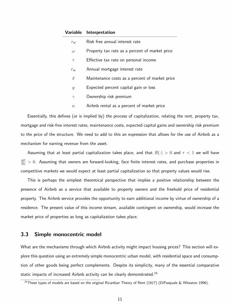
Variable Interpretation

rrf Risk free annual interest rate

ω Property tax rate as a percent of market price

τ Effective tax rate on personal income

rm Annual mortgage interest rate

δ Maintenance costs as a percent of market price

g Expected percent capital gain or loss

γ Ownership risk premium

α Airbnb rental as a percent of market price

Essentially, this defines (or is implied by) the process of capitalization, relating the rent, property tax,

mortgage and risk-free interest rates, maintenance costs, expected capital gains and ownership risk premium

to the price of the structure. We need to add to this an expression that allows for the use of Airbnb as a

mechanism for earning revenue from the asset.

Assuming that at least partial capitalization takes place, and that R(·) > 0 and τ < 1 we will have

∂P∂α

> 0. Assuming that owners are forward-looking, face finite interest rates, and purchase properties in

competitive markets we would expect at least partial capitalization so that property values would rise.

This is perhaps the simplest theoretical perspective that implies a positive relationship between the

presence of Airbnb as a service that available to property owners and the freehold price of residential

property. The Airbnb service provides the opportunity to earn additional income by virtue of ownership of a

residence. The present value of this income stream, available contingent on ownership, would increase the

market price of properties as long as capitalization takes place.

3.3 Simple monocentric model

What are the mechanisms through which Airbnb activity might impact housing prices? This section will ex-

plore this question using an extremely simple monocentric urban model, with residential space and consump-

tion of other goods being perfect complements. Despite its simplicity, many of the essential comparative

static impacts of increased Airbnb activity can be clearly demonstrated.15

15These types of models are based on the original Ricardian Theory of Rent (1817) (DiPasquale & Wheaton 1996).

11

As outlined in Figure 1, there are several ways in which Airbnb activity might impact housing prices. On

the demand side, we might reasonably expect that the Airbnb service provides homeowners with an increase

in income and as a result, more space would be demanded. Furthermore, as a result of Airbnb, there is an

increase in the population of the city demanding space or equivalently an increase in the space demanded by

each household.16 Local incomes and population may also increase if there is a localized economic impact

caused by guests spending money in areas near their Airbnb listings. Finally, there might be a negative

externality of guests, such as noise, decreased security, or simply additional demand for publicly provided

goods (such as transportation).

These comparative-static results are formally derived and well-summarized in Brueckner (1987a). Within

the context of a simple open-city model with all agents sharing a common utility function, he shows that

an increase in population is associated with an increase in rents at all locations, and an increase in income

is associated with a decline in rents for locations closer to the CBD and an increase in rents for locations

further away. Because the analysis uses an arbitrary utility function, there is no single parameter that can

represent an increase in demand.

In an effort to clarify these predictions while at the same time representing an environment that might

better approximate the limited substitutability between space and other consumption that characterizes an

thoroughly built-up area like New York City, we consider a special case of the more general model considered

in Brueckner (1987a).

Consider a “perfectly complementary” city where all households regard “space” and “other goods” as

perfect complements. The utility function will be of the form: u(α, s, o) = min(α ·s, o), where s represents

the amount of space and o represents dollars spent on other goods.17 In this model, s can be understood

as either land or interior living space; the same intuition holds. α is a preference parameter with demand

for “other goods” increasing in α and the demand for space decreasing as α increases. r is the land-rent

function, which refers to the cost of land.

Households have income, m, and all households are employed in the central business district (CBD)

16Indeed, a common anecdote among those purchasing homes is that they purchase a bigger home, one with more bedroomsfor example, because they have the ability to rent out that bedroom during peak seasons like holidays to help cover the costof a mortgage.

17The qualitative comparative statics, e.g. the sign of changes to ra, m, s, α, o, and N , do not depend on this particularutility function. Its simplicity makes it an attractive choice for a model. A more general case is presented in Brueckner(1987b).

12

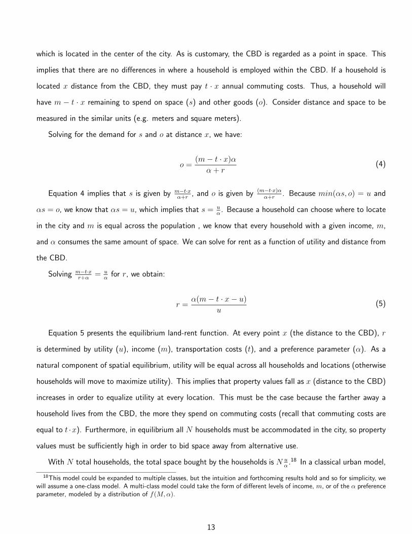
which is located in the center of the city. As is customary, the CBD is regarded as a point in space. This

implies that there are no differences in where a household is employed within the CBD. If a household is

located x distance from the CBD, they must pay t · x annual commuting costs. Thus, a household will

have m − t · x remaining to spend on space (s) and other goods (o). Consider distance and space to be

measured in the similar units (e.g. meters and square meters).

Solving for the demand for s and o at distance x, we have:

o =(m− t · x)α

α + r(4)

Equation 4 implies that s is given by m−t·xα+r

, and o is given by (m−t·x)αα+r

. Because min(αs, o) = u and

αs = o, we know that αs = u, which implies that s = uα

. Because a household can choose where to locate

in the city and m is equal across the population , we know that every household with a given income, m,

and α consumes the same amount of space. We can solve for rent as a function of utility and distance from

the CBD.

Solving m−t·xr+α

= uα

for r, we obtain:

r =α(m− t · x− u)

u(5)

Equation 5 presents the equilibrium land-rent function. At every point x (the distance to the CBD), r

is determined by utility (u), income (m), transportation costs (t), and a preference parameter (α). As a

natural component of spatial equilibrium, utility will be equal across all households and locations (otherwise

households will move to maximize utility). This implies that property values fall as x (distance to the CBD)

increases in order to equalize utility at every location. This must be the case because the farther away a

household lives from the CBD, the more they spend on commuting costs (recall that commuting costs are

equal to t ·x). Furthermore, in equilibrium all N households must be accommodated in the city, so property

values must be sufficiently high in order to bid space away from alternative use.

With N total households, the total space bought by the households is N uα

.18 In a classical urban model,

18This model could be expanded to multiple classes, but the intuition and forthcoming results hold and so for simplicity, wewill assume a one-class model. A multi-class model could take the form of different levels of income, m, or of the α preferenceparameter, modeled by a distribution of f(M,α).

13

ra represents the agricultural price of land, but we can consider ra to simply represent the opportunity

cost, or alternative use value, of land. The total land “bid away” from this use is the land area where the

price of space is greater than ra. The radius of the city, X, is determined when the value of land becomes

equal to the value of space in alternative uses, so it is therefore the maximum distance from the CBD.

The equilibrium requires that N uα

is equal to π(X)2. This is the case because the (circular) city needs to

accommodate the entire population and all space in the city will be consumed. If we set these two equal,

we can solve for the equilibrium level of utility.

X =(−Nt±

√N√Nt2 + 4mπ(ra + α))

2π(ra + α)

u =α(Nt2 + 2mπ(ra + α)−

√Nt√Nt2 + 4mπ(ra + α))

2π(ra + α)2

(6)

Because X must be positive (it is a distance), applying 6, the equilibrium land rent function is:

r = −(−m+ u+ t · x)αu

r =2mπra(ra + α) + t(−Ntα− 2πx(ra + α)2 +

√Nα√Nt2 + 4mπ(ra + α))

Nt2 + 2mπ(ra + α)−√Nt√Nt2 + 4mπ(ra + α)

(7)

We can now look at the impact of three different exogenous variables that could change as the level of

Airbnb activity increases, N,α, and m, on the land-rent function. These impacts are illustrated in Figures

2, 3, and 4. We can determine the impact of population by taking the derivative of the above land-rent

function with respect to N .

∂r

∂N=

2πt(−m+ t · x)(ra + α)2(√N√Nt2 + 4mπ(ra + α)

)(−Nt2 − 2mπ(ra + α) +

√Nt√Nt2 + 4mπ(ra + α)

) (8)

A rise in N is associated with an unambiguous increase in the value of space r at all distances x, and an

increase in the slope of the rent gradient. The land-rent function must rise to bid away additional residential

space from alternative uses in more remote parts of the city (e.g. the urban periphery). Equation 6 implies

that the increase in N results in reduced utility u, and therefore reduced consumption of space by each

household and higher population density. Spatial equilibrium requires that the value of space per unit area

decline by just enough to compensate for the extra transportation costs of households residing in that area.

14

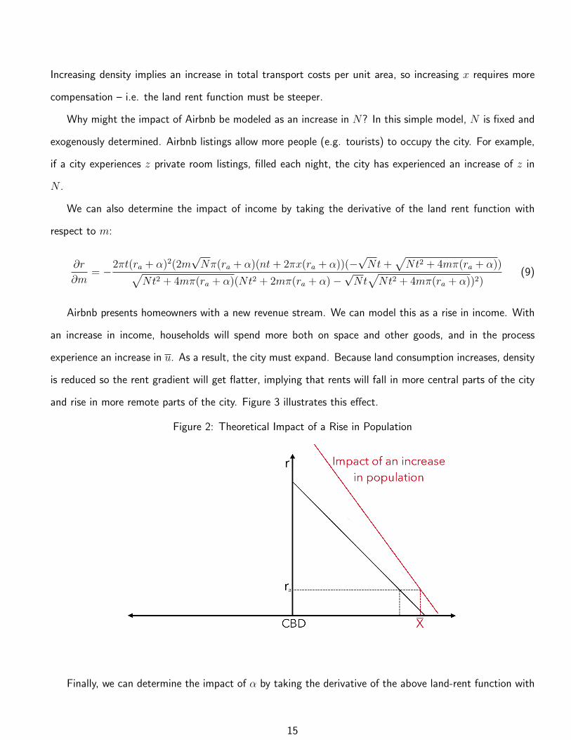
Increasing density implies an increase in total transport costs per unit area, so increasing x requires more

compensation – i.e. the land rent function must be steeper.

Why might the impact of Airbnb be modeled as an increase in N? In this simple model, N is fixed and

exogenously determined. Airbnb listings allow more people (e.g. tourists) to occupy the city. For example,

if a city experiences z private room listings, filled each night, the city has experienced an increase of z in

N .

We can also determine the impact of income by taking the derivative of the land rent function with

respect to m:

∂r

∂m= −

2πt(ra + α)2(2m√Nπ(ra + α)(nt+ 2πx(ra + α))(−

√Nt+

√Nt2 + 4mπ(ra + α))√

Nt2 + 4mπ(ra + α)(Nt2 + 2mπ(ra + α)−√Nt√Nt2 + 4mπ(ra + α))2)

(9)

Airbnb presents homeowners with a new revenue stream. We can model this as a rise in income. With

an increase in income, households will spend more both on space and other goods, and in the process

experience an increase in u. As a result, the city must expand. Because land consumption increases, density

is reduced so the rent gradient will get flatter, implying that rents will fall in more central parts of the city

and rise in more remote parts of the city. Figure 3 illustrates this effect.

Figure 2: Theoretical Impact of a Rise in Population

Finally, we can determine the impact of α by taking the derivative of the above land-rent function with

15

Figure 3: Theoretical Impact of a Rise in Income

Figure 4: Theoretical Impact of a Decrease in α

16

respect to α, which gives:

∂r

∂α= −

t(−m√N + x(

√Nt+

√Nt2 + 4mπ(ra + α))

m√Nt2 + 4mπ(ra + α)

(10)

An increase in α causes a decrease in the demand for space and vice versa. The impact we might expect as

a result of Airbnb is a decrease in α, which would cause an increase in the consumption of space as residents

purchased larger homes with seeking investment returns via short-term rentals. How does a decrease in α

impact rent? Rent in the urban periphery, e.g. in more remote parts of the city, will rise by bidding away

space from alternative uses to make available for residential housing consumption. The higher consumption

of space will reduce density which in turn will reduce the slope of the rent function r (see Figure 4). As in

the case of increasing income m, there would be a reduction in the cost of space in the city center and an

increase at the periphery. Thus, the impact of changing α does not have a uniform impact.

If an increase in Airbnb activity in a city were equivalent to a rise in N we would therefore be justified in

expecting an unambiguous rise in rent and property values, with a larger impact observed at more central

locations. On the other hand, the theoretical impacts of α and m are ambiguous so that if an increase in

Airbnb properties primarily affects the household demand for space or provides greater income there remains

an empirical question to measure the actual impacts. This provides motivation for the empirical research

presented below.

4 Data & Descriptive Statistics

Table 1 describes the different data sources used as well as their main uses. In total, there were eight main

sources of data: 1) InsideAirbnb, 2) The Department of Finance Annualized Sales Data (January 2003-

August 2015), 3) The Department of Finance “Places” or “Areas-of-Interest” Map, 4) Department of City

Planning PLUTOTM, 5) The 2010-2014 American Community Survey, 6) The New York Police Department

Crime Statistics, 7) Census Geography Maps, and 8) the Metropolitan Transportation Authority Map of

Subway Entrances.

17

Table 1: Data Sources and Use

Source Description & UseInsideAirbnb InsideAirbnb (released by Murray Cox) contains information such as

pricing, reviews, and location of each listing on Airbnb that was availableon the date the Airbnb website was crawled (12 times in 2015-2016).

Department of FinanceAnnualized Sales Data: January2003 - August 2015

The Department of Finance releases information on all sales in New YorkCity. The data are available from 2003-2015 and contain information suchas sale price, square footage,and sale date.

Department of Finance “Places”or “Areas-of-Interest” Map

The Department of Finance releases information on areas of interest, suchas parks, cemeteries, and airports, available in GIS format.

Department of City PlanningPlutoTM

The Department of City Planning releases detailed information about eachtax lot in New York City (of specific use for this analysis was squarefootage information).

American Community Survey2010-2014

The American Community Survey contains information available at theCensus Tract level such as education, racial and ethnic demographics, andemployment-related measures.

New York Police DepartmentCrime Statistics

The New York Police Department reports annual counts for differentcrimes (major felonies, non-major felonies, and misdemeanors) by precinct.

Census Geography Maps In order to merge sales with local Census demographics, Censusgeographies needed to be identified and spatially joined to the sales dataset.

Metropolitan TransportationAuthority Map of SubwayEntrances

Information provided by the Metropolitan Transportation Authority wasmade into a map of subway entrances in New York City.

Table 2 and Table 3 document descriptive statistics for the variables used in this analysis. These data

were aggregated and joined together using ArcGIS and Stata. Not all of these data are available at the same

geographic scale. For example, crime statistics were only available to us at the geographic unit of precinct,

which means that when controlling for crime for each sale, precinct is the level of granularity being used.

In all, there were 1,252,891 observations (sales) from January 2003 through August 2015. We dropped

145,594 observations because they were non-residential sales, and 319,975 observations were dropped that

had sales prices below $10,000,19 We dropped 4,533 observations with sales prices above $10,000,000,

and 2,552 observations were dropped because they were missing square footage information (or if square

footage was below 10ft or above 50,000ft), leaving a total of 780,237 observations. Approximately 16,000

observations were excluded because they could not be properly geocoded.

For each of the remaining observed sales, we have information on sale price, sale date, square footage,

and property type, along with some other variables in the Department of Finance Annualized Sales Data.

Before describing how we are calculating Airbnb activity that could influence each sale, it is important to note

the other information that was joined to the sales data. Most of the data, such as crime, Census information,

distance to subway entrances and areas-of-interest, could be spatially joined using a combination of ArcGIS

and Stata.

In the Department of Finance sales data, square footage was missing for approximately 50% of the

observations. The size of the residential property is obviously an important variable for a hedonic regression

or as a control for matching observations in a quasi-experimental approach. Rather than simply dropping

half of the observations or excluding square footage as a variable, we employed a technique using the

PLUTOTM dataset. PLUTOTM contains information on residential area (measured in square feet) and the

number of residential units by Tax Lot and Block, both of which are very small geographic units of area.

There are 857,458 Tax Lots with a mean of 1.254051 buildings per Lot. We calculated square footage

by dividing residential living area by the number of residential units in each Lot and we were then able to

join the sales data with this information to have a measure of square footage for an average unit in the

same Lot as the sale.20 While this method is not perfect, units in the same building and Lot tend to have

19Sales below $10,000 do not represent the actual sales prices of properties in New York City. Rather, they are eithermissing appropriate data or are bequests from one generation.

20For some sales, we were unable to join average square footage per Tax Lot. In these cases, we used average squarefootage per Tax Block.

19

roughly similar values and furthermore, where we had both square footage from the sales dataset and the

calculated average square footage number from PLUTOTM, the mean difference between these values for

379,673 observations was 41.68 square feet, which suggests that these measures are well within reasonable

and expected levels of accuracy.

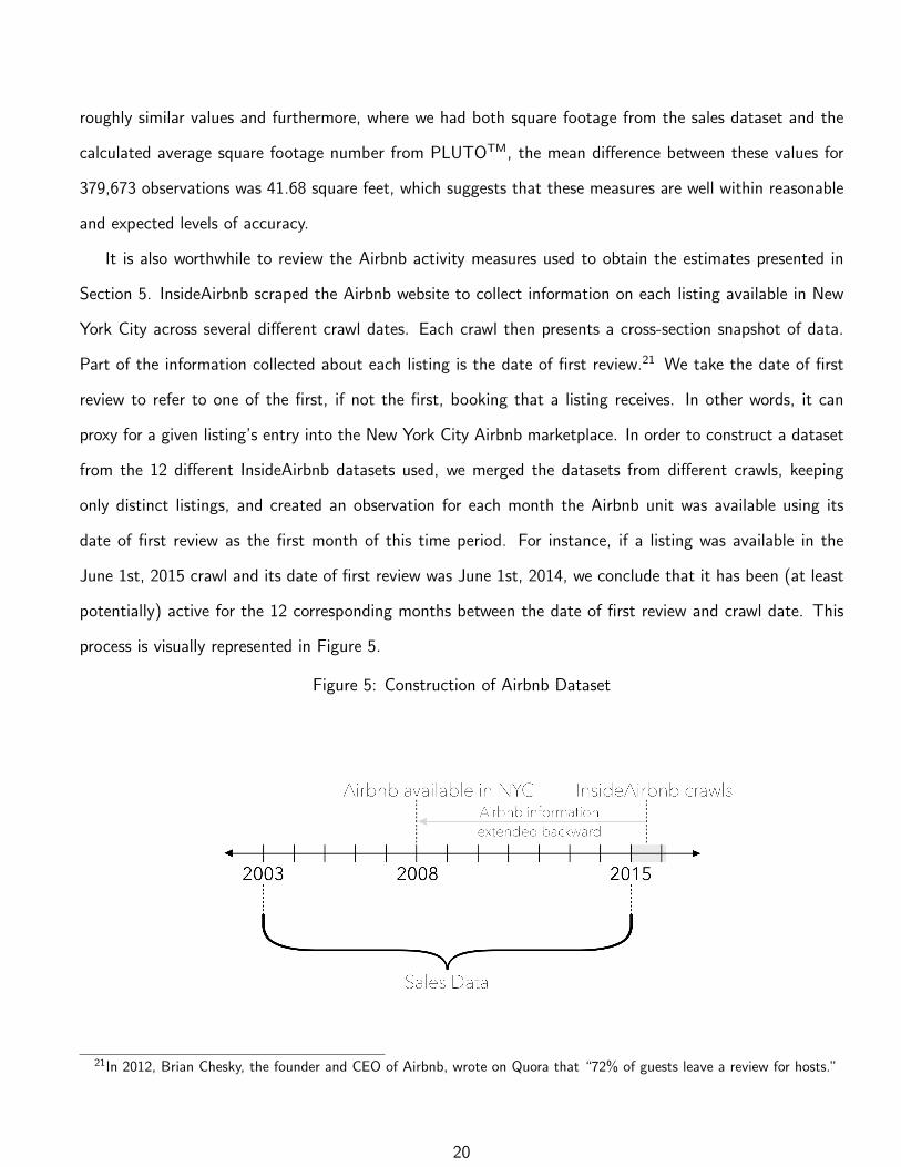
It is also worthwhile to review the Airbnb activity measures used to obtain the estimates presented in

Section 5. InsideAirbnb scraped the Airbnb website to collect information on each listing available in New

York City across several different crawl dates. Each crawl then presents a cross-section snapshot of data.

Part of the information collected about each listing is the date of first review.21 We take the date of first

review to refer to one of the first, if not the first, booking that a listing receives. In other words, it can

proxy for a given listing’s entry into the New York City Airbnb marketplace. In order to construct a dataset

from the 12 different InsideAirbnb datasets used, we merged the datasets from different crawls, keeping

only distinct listings, and created an observation for each month the Airbnb unit was available using its

date of first review as the first month of this time period. For instance, if a listing was available in the

June 1st, 2015 crawl and its date of first review was June 1st, 2014, we conclude that it has been (at least

potentially) active for the 12 corresponding months between the date of first review and crawl date. This

process is visually represented in Figure 5.

Figure 5: Construction of Airbnb Dataset

21In 2012, Brian Chesky, the founder and CEO of Airbnb, wrote on Quora that “72% of guests leave a review for hosts.”

20

This allows us to get a clear picture of Airbnb activity going back to the appearance of the first listings

when Airbnb entered the New York City market. In Figure 6, we include the number of listings over time

generated through this process.

Figure 6: Airbnb Listings Over Time

There is the possibility of measurement error with this methodology because there are hosts who enter

the Airbnb marketplace, e.g. create a listing, and then exit the market. As a result, these hosts and listings

would not be captured in our analysis unless their listing was available during one of the crawls used for

the analysis. In addition, there may be owners who make their property available on Airbnb very rarely,

and our assumption that these units are available to influence local house prices may overstate the actual

number of Airbnb properties. These sources of noise in measuring Airbnb units could result in attenuation

bias, reducing the absolute value of the estimated impact of Airbnb units on property prices.

In order to evaluate the potential impact of Airbnb activity for each sale, we created five different

buffer zones around every property sale in ArcGIS, with a radius of 150, 300, 500, 1000, and 2000 meters,

respectively. This is visually represented in Figure 7. More specifically, in Figure 7, Sale A has 1 Airbnb

listing within the first buffer zone, 4 Airbnb listings within the second buffer zone, and 11 Airbnb listings

within the third buffer zone. It is worth noting that in this calculation, we are only looking at Airbnb listings

available at the time of sale; we are able to do this because we extended Airbnb listings information back

21

until entry of Airbnb into the New York market, as discussed above. In ArcGIS, we generated Airbnb activity

measures for each sale in each of the five radii, such as number of listings, average price, and maximum

capacity. These measures are documented in Table 2. In order to do so, in ArcGIS we had to select each

sale, its corresponding Airbnb listings (available in the same month and year based on the Airbnb time series

dataset created), perform a spatial join, and export this output to Excel to later read this into Stata for an

econometric analysis. The code used for these data manipulations is available in Udell (2016).

Figure 7: Sales & Buffer Zones

Tables 2 and 3 include descriptive statistics; the first table details Airbnb activity measures and the

second details information on each sale as well as other controls used.

In total, there are 780,237 observations with corresponding Airbnb activity.22 As expected, the mean

number of listings increases with the radius of the buffer zone. There are significantly more entire home

and private room listings than there are shared room listings. There are two reasons why many entries in

the Airbnb data are recorded as zero: 1) there are sales observations from 2003 through much of 2008,

which is prior to Airbnb’s entry into the market, 2) even after Airbnb became available, there are still many

22Because the number of observations is consistent across the entire table, it is not included.

22

Table 2: Descriptive Statistics: Airbnb Activity Measures

(1) (2) (3) (4)VARIABLES mean sd min max

Listing Counts, by Total and TypeListings Count (150m) 1.221 5.217 0 133Listings Count (300m) 4.644 19.06 0 439Listings Count (500m) 11.99 47.75 0 1,034Listings Count (1000m) 40.99 157.5 0 2,899Listings Count (2000m) 133.4 490.3 0 6,170Entire Home Listings Count (150m) 0.855 3.821 0 101Entire Home Listings Count (300m) 3.249 13.91 0 309Private Room Listings Count (150m) 0.338 1.575 0 78Private Room Listings Count (300m) 1.290 5.431 0 182Shared Room Listings Count (150m) 0.0278 0.227 0 20Shared Room Listings Count (300m) 0.104 0.577 0 35

Listing CapacityAvg. Capacity (150m) 0.423 1.147 0 16Avg. Capacity (300m) 0.577 1.280 0 16Max. Capacity (150m) 3.490 15.02 0 387Max. Capacity (300m) 13.24 54.47 0 1,215Avg. Bedrooms (150m) 0.158 0.430 0 10Avg. Bedrooms (300m) 0.305 0.713 0 16Sum Bedrooms (150m) 1.302 5.616 0 136Sum Bedrooms (300m) 4.951 20.37 0 459Sum Beds (150m) 1.819 7.841 0 294Sum Beds (300m) 6.899 28.21 0 622

Listing PriceAvg. Nightly Price (150m) 23.09 65.18 0 5,000Avg. Nightly Price (300m) 29.34 69.00 0 5,000Sum Price (150m) 213.744 989.79 0 25,308Sum Price (300m) 813.8 3,617 0 74,874Median Price (150m) 19.85 57.81 0 5,000Median Price (300m) 24.69 60.49 0 5,000

ReviewsSum Reviews (150m) 31.77 140.4 0 4,396Sum Reviews (300m) 122.0 499.6 0 11,5999

23

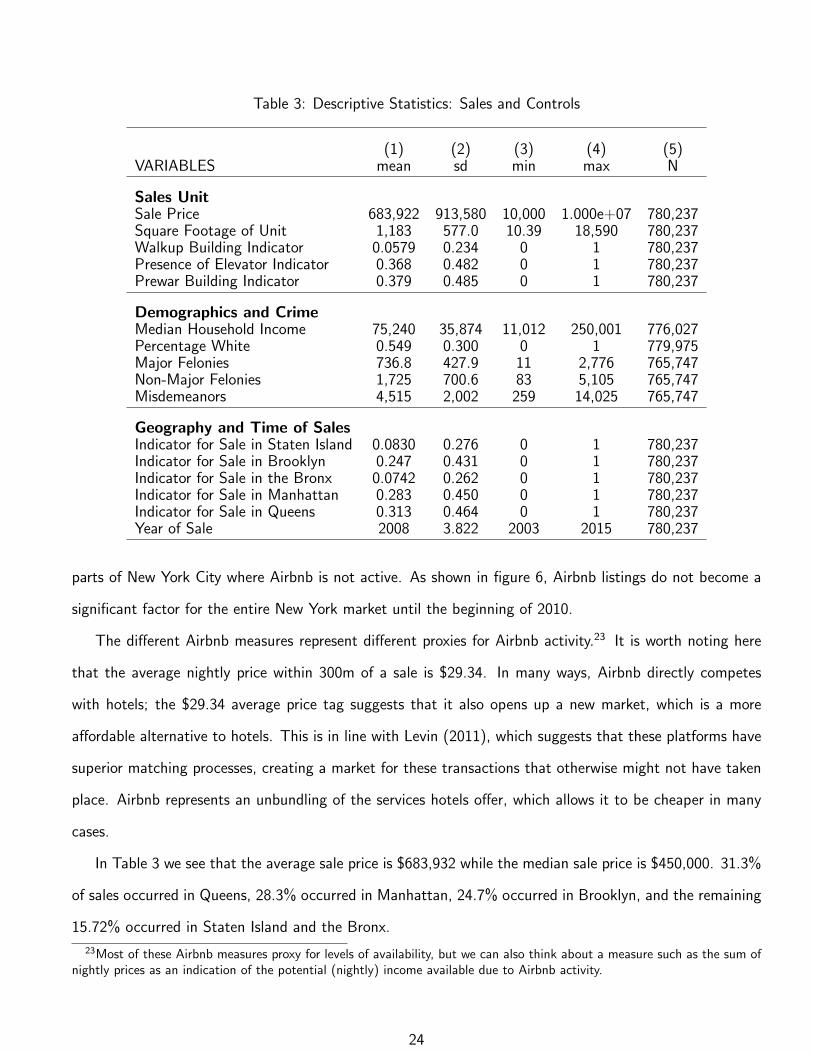
Table 3: Descriptive Statistics: Sales and Controls

(1) (2) (3) (4) (5)VARIABLES mean sd min max N

Sales UnitSale Price 683,922 913,580 10,000 1.000e+07 780,237Square Footage of Unit 1,183 577.0 10.39 18,590 780,237Walkup Building Indicator 0.0579 0.234 0 1 780,237Presence of Elevator Indicator 0.368 0.482 0 1 780,237Prewar Building Indicator 0.379 0.485 0 1 780,237

Demographics and CrimeMedian Household Income 75,240 35,874 11,012 250,001 776,027Percentage White 0.549 0.300 0 1 779,975Major Felonies 736.8 427.9 11 2,776 765,747Non-Major Felonies 1,725 700.6 83 5,105 765,747Misdemeanors 4,515 2,002 259 14,025 765,747

Geography and Time of SalesIndicator for Sale in Staten Island 0.0830 0.276 0 1 780,237Indicator for Sale in Brooklyn 0.247 0.431 0 1 780,237Indicator for Sale in the Bronx 0.0742 0.262 0 1 780,237Indicator for Sale in Manhattan 0.283 0.450 0 1 780,237Indicator for Sale in Queens 0.313 0.464 0 1 780,237Year of Sale 2008 3.822 2003 2015 780,237

parts of New York City where Airbnb is not active. As shown in figure 6, Airbnb listings do not become a

significant factor for the entire New York market until the beginning of 2010.

The different Airbnb measures represent different proxies for Airbnb activity.23 It is worth noting here

that the average nightly price within 300m of a sale is $29.34. In many ways, Airbnb directly competes

with hotels; the $29.34 average price tag suggests that it also opens up a new market, which is a more

affordable alternative to hotels. This is in line with Levin (2011), which suggests that these platforms have

superior matching processes, creating a market for these transactions that otherwise might not have taken

place. Airbnb represents an unbundling of the services hotels offer, which allows it to be cheaper in many

cases.

In Table 3 we see that the average sale price is $683,932 while the median sale price is $450,000. 31.3%

of sales occurred in Queens, 28.3% occurred in Manhattan, 24.7% occurred in Brooklyn, and the remaining

15.72% occurred in Staten Island and the Bronx.

23Most of these Airbnb measures proxy for levels of availability, but we can also think about a measure such as the sum ofnightly prices as an indication of the potential (nightly) income available due to Airbnb activity.

24

The descriptive statistics presented in tables 2 and 3 allow us to make a quick “back of the envelope”

calculation of the potential impact on property values. Consider the income capitalization approach outlined

in section 3. Airbnb imposes a host fee of 3% of the rental value, in addition to the guest fees that are

added to the nightly rental. It seems reasonable to expect that there will be many nights when the property

is not rented, but suppose an optimistic owner of an average property expects to be able to rent 330 nights

per year. Then the total annual Airbnb income expected would be $29.34×330×0.97 = $9392. Combining

this figure with the mean property value of $683,922 this implies a value of α = 0.01373 for equation 3.

For other variables in equation 3, we assume that g = γ (the expected capital gain equals the ownership

risk premium) and apply reasonable estimates to other variables as follows:

Variable Value Interpretation

rrf 0.02 Risk free annual interest rate

ω 0.025 Property tax rate as a percent of market price

τ 0.29 Effective tax rate on personal income

rm 0.04 Annual mortgage interest rate

δ 0.025 Maintenance costs as a percent of market price

α 0.01373 Airbnb rental as a percent of market price

Using these values in both equations 2 and 3, we can calculate that the availability of Airbnb rentals has

diminished the user cost of housing by about 17.7%. If utility levels in the city remain constant (as would

be expected in long-run equilibrium of an open city), and given unchanged transport costs and preferences,

we would expect rents per unit of space to remain unchanged. This reduction in the user cost of housing

would then imply, via equation 1 a 17.7% increase in the price of housing.

These calculations are at best an approximation of what we might expect to observe. Not all portions

of the city are equally exposed to Airbnb activity and market equilibrium may take years to be realized.

Nevertheless, the calculation provides some intuition about the potential magnitude of price impacts.

Not all portions of the city have the same intensity of Airbnb listings. Figure 8 shows the distribution of

Airbnb listings (from any time period) across the city, with dots color coded by daily price. It can be difficult

from the map to tell how dense the coverage is, so an inset showing midtown Manhattan is provided. This

suggests that as of late 2015, coverage in the areas of the city with greatest demand for lodging is very

complete.

25

Figure 8: Airbnb listings in New York City, with inset showing midtown Manhattan

26

5 Empirical Estimates

We employ two distinct approaches to estimating the impacts of Airbnb properties on house prices. First,

we employ a relatively traditional hedonic approach as presented and explained in Rosen (1974) or Sheppard

(1999) and widely used to measure the importance of factors affecting property values. Second, we employ

several quasi-experimental approaches to identify treatment and control groups within the observational

data, and then estimate the average treatment effect generated by the Airbnb quasi-experiment.

The first approach provides a measure of the associational impact of Airbnb – the change in values that

an observant buyer might detect as the housing market adapts and responds. It cannot, however, pretend

to provide an analog to the causal impact obtained from a controlled experiment in which the sales price of

identical (or very similar) structures are compared after one of them (the treated property) is subject to the

impact of locally available Airbnb rentals while the other (the control) is not subject to these local impacts.

Because we are fortunate to have a very large number of individual sales observations, we can apply these

techniques to identify the experimental data within the large observational data. This offers the prospect of

measuring a causal impact, and it is worth distinguishing between this approach and the use of instrumental

variables that are widely applied in response to concerns about endogenous variables. Instrumental variable

approaches can (in ideal circumstances) reduce endogeneity bias in estimating associational relations, but

cannot be relied upon to measure causal impacts.

Our unit of observation is an individual sale that took place in New York City (five boroughs) between

January 2003 and August 2015. We therefore have a large number of sales both before and after Airbnb units

become actively available.24 For each sale, we include controls for the property itself, the building in which

it is located, local amenities (such as access to public transportation), local neighborhood characteristics

(demographics and crime), a year of sale fixed effect to capture a time trend of sales prices, and a local

neighborhood fixed effect to capture time invariant neighborhood quality or desirability. For each sale, we

calculate a level of local Airbnb activity, which is the main variable of interest, and corresponds to Airbnb

activity at the time of sale. In most specifications, this Airbnb activity is proxied by the number of listings,

24It is worth noting that the sales are nominal rather than real prices. we include year of sale fixed effects to deal withthis problem. This is, in fact, preferable to using a house price index to determine “real prices” because available house priceindices generally cover a different geographic area than our data.

We compare the index, which is constructed from the estimates on the year of sale fixed effects, to the S&P/Case-ShillerNY, NY Home Price Index to demonstrate its plausibility.

27

but we present estimates that use alternative indices of Airbnb activity as well.

There are two main assumptions of the hedonic identification strategy: 1) with regards to generating the

Airbnb dataset, we are assuming that the date of first review indicates when a property became available

on Airbnb and that once it became available, it never exited the Airbnb market. This allows us to construct

a dataset of Airbnb activity over time and calculate local Airbnb activity at the time of sale and 2) local

neighborhood fixed effects capture time-invariant local neighborhood quality. If these assumptions are valid,

these estimates will reveal the impact of local Airbnb activity on sales prices. If these assumptions hold,

because we are controlling for property, building, and neighborhood characteristics, the only thing that is

changing is local Airbnb activity (as well as the overall level of the market, which is captured by year of sale

fixed effects).

The specification we are using in the baseline model follows the form:

ln(Sale Priceicmt) = α + β1ln(Airbnb Activityim) + µ1(Property Characteristicsi)+

µ2(Building Controlsi) + µ3(Demographic and Crime Controlsit)+

µ4(Year of Sale FEit) + µ5(Local Neighborhood FEic) + εicmt

(11)

where ln(Sale Priceicmt) is equal to the logarithm of property i’s sale price, in neighborhood c, in month

m, and year t, and where β represents a scalar coefficient and µ represents a vector coefficient.

The independent variable is the natural log of sale price. The main variable of interest is Airbnb activity

(proxied by different descriptive and proximate measures of Airbnb, as will be discussed in Section 5). For

each sale, square footage, distance to the nearest subway entrance and area of interest are used as well as

controls for the building, year of sale, local crime, and local demographics. In the model, a time-invariant

local neighborhood fixed effect is included to capture unobservable or uncontrolled for local neighborhood

quality and characteristics. There is significant evidence that housing prices are heavily influenced by the

characteristics of a neighborhood as well as surrounding land use (DiPasquale & Wheaton 1996, p. 349).

As with most microeconometric estimation, there are natural concerns regarding endogeneity of right-

hand side variables. We are not estimating the individual household demand for the characteristic of

proximity to Airbnb properties or for listing a property on Airbnb, so the traditional concerns regarding

endogeneity of individual household decisions discussed in Sheppard (1999) do not arise. Endogeneity may

nevertheless be a valid concern if important factors affecting house prices are correlated with the unobserved

28

errors in the hedonic equation. Thus, for example, if errors ε in the hedonic price function are correlated

with measured values of right-hand side variables in equation 11 then estimates may be biased.

For example, we might expect increasing Airbnb activity to be correlated with the error term of the

hedonic if the number of Airbnb properties within a given buffer distance were positively related to unob-

served errors ε. Note that the problem does not involve a correlation between Airbnb activity and property

values. The problem arises if we have correlation between Airbnb activity and ε, which is the component of

property value that is not explained by the hedonic.

Proving there is no such relationship is extremely difficult. There are several considerations that we

suggest as a basis for regarding our hedonic estimates as reasonable: 1) we include sales data prior to

Airbnb’s entry into the New York City market and therefore have at least five years of data (2003 through

most of 2008), where sales are not subject to any Airbnb “treatment,”25 2) local neighborhood fixed

effects, which in our preferred specification are at the level of Census Block-Group, and 3) use of robust

standard errors, which in our preferred specification are clustered at the level of Census Tract, to help deal

with correlation within clusters and heteroskedasticity. Finally, even if we expected there to be correlation

between unexplained errors ε in the hedonic model and the number of Airbnb properties very near to the

source of error, this correlation should be greatly reduced as we consider larger buffer areas. A distance

exceeding 1,000 meters in the New York housing market is generally large enough to be associated with

significant neighborhood change. As noted in section 4, these larger buffer areas also involve many more

properties, and it strains credulity that the number of Airbnb properties within a kilometer in any direction

would be significantly affected by an unusually under- or over-valued property sale.

While this approach is not immune from endogeneity concerns and makes other implicit assumptions

concerning stability of trends, the central role of the treatment variable interacted with the indicator for the

time period after which any treatment is delivered, coupled with the reduced likelihood that this interaction

variable is correlated with the unobserved ε in the model make presentation of these estimates worthwhile.

A final check is provided by comparing the estimates of the “preferred” models from each approach with

the intuitive “back of the envelope” calculations presented in section 4 will be instructive as indicators of

the reasonableness of the estimates.

25Therefore, the change we are identifying, controlling for property and local neighborhood characteristics as well as theoverall level of the market, should be attributable solely to Airbnb activity.

29

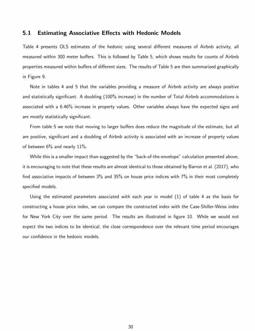
5.1 Estimating Associative Effects with Hedonic Models

Table 4 presents OLS estimates of the hedonic using several different measures of Airbnb activity, all

measured within 300 meter buffers. This is followed by Table 5, which shows results for counts of Airbnb

properties measured within buffers of different sizes. The results of Table 5 are then summarized graphically

in Figure 9.

Note in tables 4 and 5 that the variables providing a measure of Airbnb activity are always positive

and statistically significant. A doubling (100% increase) in the number of Total Airbnb accommodations is

associated with a 6.46% increase in property values. Other variables always have the expected signs and

are mostly statistically significant.

From table 5 we note that moving to larger buffers does reduce the magnitude of the estimate, but all

are positive, significant and a doubling of Airbnb activity is associated with an increase of property values

of between 6% and nearly 11%.

While this is a smaller impact than suggested by the “back-of-the-envelope” calculation presented above,

it is encouraging to note that these results are almost identical to those obtained by Barron et al. (2017), who

find associative impacts of between 3% and 35% on house price indices with 7% in their most completely

specified models.

Using the estimated parameters associated with each year in model (1) of table 4 as the basis for

constructing a house price index, we can compare the constructed index with the Case-Shiller-Weiss index

for New York City over the same period. The results are illustrated in figure 10. While we would not

expect the two indices to be identical, the close correspondence over the relevant time period encourages

our confidence in the hedonic models.

30

Table 4: OLS estimates of Airbnb impacts

(1) (2) (3) (4)

Variables ln(Sale Price) ln(Sale Price) ln(Sale Price) ln(Sale Price)

Total Accommodations 0.0646***

0.00275

Total Reviews 0.0393***

0.00173

Total Rooms 0.0814***

0.00351

Total Rents 0.0323***

0.00133

Square Feet 0.402*** 0.402*** 0.402*** 0.402***

0.0178 0.0178 0.0178 0.0178

Felonies -0.0458*** -0.0552*** -0.0455*** -0.0517***

0.0161 0.0162 0.0162 0.0161

Pre-war 0.0843*** 0.0846*** 0.0842*** 0.0847***

0.0111 0.0111 0.0111 0.0111

Distance to AOI -0.103 -0.101 -0.103 -0.102

0.0674 0.0674 0.0675 0.0674

Distance to subway -0.00875 -0.00880 -0.00897 -0.00897

0.0243 0.0241 0.0243 0.0242

Elevator 0.0858*** 0.0849*** 0.0863*** 0.0847***

0.0235 0.0235 0.0235 0.0234

Y2004 0.179*** 0.180*** 0.178*** 0.180***

0.0121 0.0119 0.0121 0.0120

Y2005 0.365*** 0.367*** 0.365*** 0.366***

0.0127 0.0126 0.0128 0.0126

Y2006 0.464*** 0.467*** 0.464*** 0.466***

0.0164 0.0159 0.0164 0.0161

*** - significant at 1%, ** - significant at 5%, * - significant at 10%

Continued on next page

31

... continued from previous page:

(1) (2) (3) (4)

Variables ln(Sale Price) ln(Sale Price) ln(Sale Price) ln(Sale Price)

Y2007 0.490*** 0.492*** 0.490*** 0.491***

0.0179 0.0175 0.0179 0.0177

Y2008 0.465*** 0.467*** 0.465*** 0.466***

0.0192 0.0188 0.0192 0.0190

Y2009 0.341*** 0.338*** 0.343*** 0.339***

0.0171 0.0178 0.0170 0.0174

Y2010 0.352*** 0.345*** 0.356*** 0.344***

0.0184 0.0182 0.0185 0.0181

Y2011 0.311*** 0.297*** 0.318*** 0.296***

0.0160 0.0165 0.0161 0.0160

Y2012 0.344*** 0.336*** 0.351*** 0.333***

0.0157 0.0150 0.0160 0.0152

Y2013 0.325*** 0.323*** 0.331*** 0.318***

0.0143 0.0132 0.0146 0.0137

Y2014 0.389*** 0.401*** 0.394*** 0.391***

0.0138 0.0125 0.0140 0.0132

Y2015 0.432*** 0.455*** 0.436*** 0.437***

0.0151 0.0137 0.0152 0.0143

Constant 10.84*** 10.88*** 10.84*** 10.87***

0.490 0.498 0.490 0.494

Observations 765,747 765,747 765,747 765,747

R-squared 0.524 0.524 0.524 0.524

Sale-Year FE YES YES YES YES

Local Neighborhood FE Census Block Group Census Block Group Census Block Group Census Block Group

Clustered Standard Errors Census Tract Census Tract Census Tract Census Tract

*** - significant at 1%, ** - significant at 5%, * - significant at 10%

32

Table 5: OLS estimates of Airbnb impacts with increasing buffer sizes

(1) (2) (3) (4) (5)

Variables ln(Sale Price) ln(Sale Price) ln(Sale Price) ln(Sale Price) ln(Sale Price)

Airbnb150 0.109***

0.00555

Airbnb300 0.0879***

0.00377

Airbnb500 0.0773***

0.00309

Airbnb1000 0.0670***

0.00261

Airbnb2000 0.0601***

0.00249

Sauare Feet 0.403*** 0.403*** 0.403*** 0.402*** 0.402***

0.0180 0.0179 0.0179 0.0179 0.0179

Felonies -0.0574*** -0.0363** -0.0268* -0.0243 -0.0307*

0.0171 0.0161 0.0159 0.0156 0.0158

Pre-war 0.0838*** 0.0838*** 0.0839*** 0.0842*** 0.0840***

0.0112 0.0112 0.0112 0.0112 0.0112

Distance to AOI -0.0993 -0.100 -0.100 -0.0997 -0.0991

0.0770 0.0770 0.0768 0.0772 0.0770

Distance to subway -0.00978 -0.00931 -0.00984 -0.0111 -0.0113

0.0251 0.0250 0.0249 0.0249 0.0248

Elevator 0.0904*** 0.0907*** 0.0907*** 0.0903*** 0.0902***

0.0239 0.0239 0.0239 0.0238 0.0238

Y2004 0.180*** 0.177*** 0.176*** 0.175*** 0.176***

0.0122 0.0121 0.0119 0.0118 0.0116

Y2005 0.366*** 0.363*** 0.362*** 0.362*** 0.363***

0.0129 0.0127 0.0125 0.0123 0.0122

*** - significant at 1%, ** - significant at 5%, * - significant at 10%

Continued on next page

33

... continued from previous page:

(1) (2) (3) (4) (5)

Variables ln(Sale Price) ln(Sale Price) ln(Sale Price) ln(Sale Price) ln(Sale Price)

Y2006 0.465*** 0.462*** 0.461*** 0.461*** 0.462***

0.0168 0.0164 0.0161 0.0159 0.0157

Y2007 0.490*** 0.488*** 0.488*** 0.488*** 0.489***

0.0181 0.0180 0.0177 0.0176 0.0175

Y2008 0.465*** 0.464*** 0.463*** 0.464*** 0.465***

0.0194 0.0193 0.0191 0.0190 0.0189

Y2009 0.345*** 0.341*** 0.338*** 0.330*** 0.316***

0.0168 0.0171 0.0171 0.0170 0.0168

Y2010 0.360*** 0.354*** 0.346*** 0.331*** 0.313***

0.0185 0.0185 0.0184 0.0180 0.0174

Y2011 0.328*** 0.307*** 0.286*** 0.255*** 0.219***

0.0156 0.0159 0.0160 0.0155 0.0148

Y2012 0.359*** 0.327*** 0.303*** 0.269*** 0.228***

0.0161 0.0159 0.0152 0.0145 0.0135

Y2013 0.364*** 0.328*** 0.302*** 0.265*** 0.220***

0.0150 0.0147 0.0142 0.0136 0.0129

Y2014 0.421*** 0.385*** 0.357*** 0.317*** 0.269***

0.0144 0.0142 0.0137 0.0132 0.0128

Y2015 0.467*** 0.428*** 0.398*** 0.355*** 0.308***

0.0156 0.0155 0.0149 0.0148 0.0147

Constant 10.88*** 10.75*** 10.70*** 10.69*** 10.73***

0.545 0.547 0.548 0.552 0.553

Observations 742,328 742,328 742,328 742,328 742,328

R-squared 0.524 0.524 0.525 0.525 0.525

Local Neighborhood FE Census Block Group Census Block Group Census Block Group Census Block Group Census Block Group

Clustered Standard Errors Census Tract Census Tract Census Tract Census Tract Census Tract

*** - significant at 1%, ** - significant at 5%, * - significant at 10%

34

Figure 9: Airbnb impacts for different buffer sizes

Figure 10: Comparison of house price index from Airbnb model with CSW index

35

5.2 Quasi-Experimental Estimation of Airbnb Treatment Effects

The results presented in the preceding subsection cannot be given a clear causal interpretation. Hedonic

models present the association observed in equilibrium between structure and neighborhood characteristics

(such as the presence of Airbnb properties within 300 meters of the property) and the recorded sale price. As

noted in Sheppard (1999) the hedonic price function arises from the interaction of supply and consumption

choices made in the housing market and describes a locus of equilibrium outcomes rather than a behavioral

or causal link.

To properly evaluate the causal impact of Airbnb properties on house prices, we would ideally have a

controlled experiment in which identical properties were identified, one of them exposed to the treatment of

having nearby Airbnb properties and one of them insulated from this treatment, and the sales prices could

then be compared over a sample of properties to estimate the impact on house prices caused by Airbnb.

The impracticality of conducting such an experiment is obvious, but our observational data permit

application of widely-used26 quasi-experimental approaches. These approaches permit us, given certain

assumptions, to identify the experimental information that are contained within our observational data and

to approximate a controlled experimental design. The large size and extensive time over which our data are

observed make this a particularly appropriate methodology for application.

We employ three methods for evaluating treatment effects: construction of treatment and control

groups based on nearest-neighbor matching, based on propensity-score matching, and the use of regression

adjustment for determination of treatment and control groups.

Table 6 provides the estimated treatment effects, based on sales prices adjusted for prevailing property

price levels using the Case-Shiller-Weiss house price index for New York City. Note that ‘treatment’ here

means that the sale of a residential property took place at a time when there were Airbnb properties available

within 300 meters of the sale property location. The first rows present estimates making use of all properties

with full data in the sample, without regard to location. Subsequent rows, as noted in the first column,

break the data into subsamples based on the distance between the sale property and the CBD, here taken

to be Wall Street in lower Manhattan.

The first column of average treatment effect estimates is obtained using nearest-neighbor matched pairs

26See discussion and references in Chapter 21 of Wooldridge (2010) or Chapters 1 and 2 of Cerulli (2015).

36

based on the Mahalanobis distance between observations, applying large-sample bias correction. Beneath

estimate of treatment effects is the estimated standard error. The second column presents estimates of

average treatment effects constructing treatment and control groups using propensity score matching. The

third column presents estimated average treatment effects using regression adjustment, followed by the

mean potential outcome for the data and the number of observations.

In every case, the estimated standard errors are very small so that estimated precision of the estimates is

high. Estimated treatment effects on the population are generally somewhat higher than the associational

estimates obtained using the hedonic models or our ‘back-of-the-envelope’ calculations, ranging from a nearly

21% impact estimated using nearest-neighbor comparisons to nearly 35% using regression adjustment.

Table 6: Estimated effect of treatment: presence of Airbnb property within 300 meters

Nearest Propensity Regression Mean PotentialNeighbor Score Adjustment Outcome Observations

All distances 0.2094*** 0.3171*** 0.3493*** 13.0494*** 710,422σ 0.007 0.006 0.003 0.001

Less than 7 km 0.3252*** 0.5142*** 0.5490*** 13.1592*** 171,815σ 0.058 0.014 0.005 0.004

7 km to 11.5 km 0.2405*** 0.3113*** 0.2854*** 13.2848*** 189,492σ 0.057 0.008 0.005 0.002

11.5 km to 17 km 0.1734*** 0.2774*** 0.1678*** 12.8657*** 166,121σ 0.020 0.011 0.007 0.002

More than 17 km 0.1051*** 0.0490*** 0.0428*** 12.9035*** 182,994σ 0.024 0.014 0.010 0.002

*** - significant at 1 percent

Our data include an extended time period during which there were no treated properties. The very first

treated sales occur in 2008 but, as noted above and illustrated in Figure 6, most treated sales take place

after the beginning of 2010. Even in 2012 the majority of property sales are not within 300 meters of a

property ever available on Airbnb and hence ‘untreated’.

For all estimation approaches, we see that the average treatment effects are higher for properties located

closer to the commercial center, and lower for those properties located further away. This is not simply an

artifact of more intense treatment (in the sense of proximity to more Airbnb properties) for more centrally

located sales. Table 7 presents a set of estimated treatment effects for the population that distinguishes

between different intensities of treatment.

37

As expected, we see that for all distances (the first column of estimates) the treatment effect rises with

intensity of treatment. Properties sold within 300 meters of 1 to 5 Airbnb properties sell for about 16%

more, while those exposed to 31 or more properties sell for a 77% premium. This general pattern holds

within distance bands as well. Average treatment effects rise with treatment intensity for properties within

7 kilometers of the center as well as for those further out. In addition, restricting attention to a particular

treatment intensity and moving along the row (to more distant properties) shows again that the treatment

effect tends to decline. Thus, for example, a property exposed to between 6 and 10 Airbnb properties sells

for a 58% premium within 7 km of the center, and the treatment effect diminishes as we consider properties

further from the center (but exposed to the same intensity of treatment).

Figure 11 illustrates these results. The diagram shows a dot for each value in Table 7, and we see that

within each color group (distance from the center) the estimated treatment effect rises with the intensity

of treatment. We also see that, in general, the red dots (closest to CBD) are higher than the blue, which in

turn are higher than the green. This indicates that the increase in house prices (and presumably the price

of space) is greater at central locations and diminishes as we move towards the periphery of the city.

Table 7: Estimated effect of different treatment levels

# Airbnb All Distances Less than 7km 7km to 11.5km 11.5km to 17km More than 17km

1 to 5 0.1596*** 0.1413*** 0.1653*** 0.0855*** 0.0354 ***σ 0.004 0.010 0.006 0.007 0.011

6 to 10 0.4553*** 0.5838*** 0.3371*** 0.2202*** -0.0522σ 0.012 0.010 0.012 0.046 0.125

11 to 15 0.5399*** 0.6486*** 0.4228*** -0.1171σ 0.030 0.012 0.019 0.194

16 to 20 0.6636*** 0.6712*** 0.4999*** 0.4179*σ 0.035 0.014 0.023 0.241

21 to 25 0.6403*** 0.6699*** 0.5361*** -0.0761σ 0.037 0.015 0.027 0.237

26 to 30 0.6436*** 0.6499*** 0.5379*** -0.3063σ 0.043 0.019 0.034 0.365

31 or more 0.7748*** 0.7934*** 0.5903*** -0.0325σ 0.018 0.007 0.016 0.173

*** - significant at 1 percent, * - significant at 10 percent

38

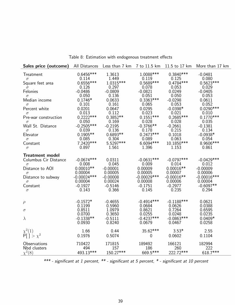
Table 8: Estimation with endogenous treatment effects

Sales price (outcome) All Distances Less than 7 km 7 to 11.5 km 11.5 to 17 km More than 17 km

Treatment 0.6456*** 1.3613 1.0088*** 0.3840*** -0.0481σ 0.114 1.449 0.119 0.125 0.080

Square feet area 0.6556*** 1.0315*** 0.5689*** 0.4784*** 0.5623***σ 0.126 0.297 0.078 0.053 0.029

Felonies -0.0486 -0.0809 -0.0821 0.0249 -0.0405σ 0.050 0.136 0.051 0.050 0.053

Median income 0.1746* 0.0633 0.3363*** -0.0298 0.0611σ 0.101 0.161 0.065 0.053 0.052

Percent white 0.0201 0.0647 0.0295 -0.0398* 0.0290***σ 0.013 0.112 0.023 0.021 0.010

Pre-war construction 0.2222*** 0.3852** 0.1551*** 0.2685*** 0.1770***σ 0.050 0.169 0.028 0.028 0.035

Wall St. Distance -0.2505*** -0.2195 -0.3766** -0.2661 -0.1381σ 0.039 0.136 0.178 0.215 0.134

Elevator 0.1905** 0.6893** 0.2473*** 0.1018 -0.0938*σ 0.085 0.304 0.089 0.063 0.054

Constant 7.2420*** 5.5297*** 6.6094*** 10.1850*** 8.9606***σ 0.897 1.561 1.396 1.153 0.861

Treatment modelColumbus Cir Distance -0.0674*** 0.0311 -0.0631*** -0.0797*** -0.0429***σ 0.008 0.045 0.009 0.014 0.012

Distance to AOI 0.00010** -0.00001 0.00009 0.00016** -0.00009σ 0.00004 0.00005 0.00005 0.00007 0.00006

Distance to subway -0.00024*** -0.00008 -0.00029*** -0.00016** -0.00016***σ 0.00004 0.00024 0.00008 0.00006 0.00004

Constant -0.1927 -0.5146 -0.1751 -0.2977 -0.6097**σ 0.143 0.366 0.145 0.235 0.294

ρ -0.1572* -0.4655 -0.4914*** -0.1188*** 0.06210.1199 0.5960 0.0684 0.0626 0.0388

σ 0.8511 1.0979 0.8621 0.7264 0.65950.0700 0.3650 0.0255 0.0248 0.0235

λ -0.1338** -0.5111 -0.4237*** -0.0863*** 0.0409*0.0930 0.8240 0.0679 0.0467 0.0258

χ2(1) 1.66 0.44 35.62*** 3.53* 2.55P[ ] > χ2 0.1976 0.5074 0 0.0602 0.1104

Observations 710422 171815 189492 166121 182994Nbd clusters 494 157 186 260 222χ2(8) 493.13*** 150.27*** 669.5*** 222.72*** 618.7***

*** - significant at 1 percent, ** - significant at 5 percent, * - significant at 10 percent

39

Figure 11: Impact on house prices of different treatment levels at various distances

There is a natural concern that these results may be an artifact of some endogeneity in the treatment

of properties. This is not a fully randomized assignment of treatment to similar properties, and it may be

that (despite the results presented in Table 7) some element of high-demand locations might be subjecting

properties closer to the CBD to more intense treatment. We consider the possibility that these impacts

may be distorted by endogeneity of treatment, and present the resulting estimates in Table 8.

As expected, the more demanding estimation approach results in somewhat less precise estimates, but

overall the results are quite comparable to those presented in the previous tables. The treatment model

considers three measures of location advantage to identify areas where treatment is more likely. Distance

from Columbus Circle, distance to other areas of interest identified by the Department of Finance, and

distance to the nearest subway station. Only distance to Columbus Circle and to the nearest subway station

are typically estimated with precision. The models cluster standard errors by neighborhood.

Overall, the results suggest average treatment effects that are larger in the central locations and diminish

(to the point of insignificance) as we move towards the periphery of the city. For all distances combined,

the average treatment effect indicates a 64% premium for treated sales taking place within 300 meters of

40

other properties that are available via Airbnb.

Interestingly, the estimated correlation ρ is negative, indicating that unobservable factors that increase

property sales prices tend to occur with unobservables that decrease the chance of nearby Airbnb properties.

This increases our confidence that the estimated average treatment effects are not merely an artifact of

endogenous treatment probabilities, even in those distance bands where the chi-square test indicates that

we must reject the hypothesis of no endogeneity in treatment selection.

6 Conclusions

In this paper we have presented a variety of estimates of the impacts that properties listed for rent on

Airbnb appear to have on the market value of residential properties in New York City. The direction and

magnitude of these impacts has prompted widespread concern and considerable debate about the impact

on urban structure and housing affordability in New York City and in other cities around the world. Many

jurisdictions have responded by attempting to regulate or impose restrictions on the ability of Airbnb to

operate or of property owners to makes use of Airbnb services.

We present intuitive and formal theoretical arguments that generally support, but do not ensure that

this impact would be for house prices to increase in response to Airbnb listings as long as the Airbnb

properties themselves are not the source of extensive or concentrated negative externalities. This impact

is not guaranteed, however, and empirical investigation is required to determine the sign and magnitude of

impact.

Our theoretical arguments suggest two possibilities: an increase in property values throughout the city

that is greater in the center than at the periphery (if Airbnb properties facilitate an increase in population

accommodated in the city), an increase in property values that is greater at the urban periphery and

diminishes (or is negative) at the urban center (if Airbnb brings increased income to residents or increases

the demand for space for each household). The first possibility is associated with a decline in equilibrium

utility levels of residents. The second with an increase in utility.

We have presented several estimates of the likely range of impacts. A quick ‘back-of-the-envelope’

calculation based on income capitalization suggests that property values should increase about 17%. Hedonic

analysis of house prices indicates that a doubling of the total number of Airbnb properties within 300 meters

41

of a house is associated with an increase in property value of 6% to 9% (depending on model specification).

Consideration of the introduction of Airbnb as an experimental treatment to the housing market, and

estimation of average treatment effects provides the most satisfactory approach to evaluation of the impacts

of Airbnb on house prices. Our analysis indicates that subjecting a property to the treatment of having

Airbnb properties available nearby when it is sold increases prices by 3.5% (for properties that are far from

the center and whose ‘treatment’ consists of only a few Airbnb properties) to more than 65% for properties

that are near the center and/or are ‘treated’ by having a larger number of local Airbnb properties.

Somewhat more speculatively, we note that our analysis is consistent with thinking of Airbnb as increasing

local urban population (by attracting tourists), since this would generate a pattern of property value changes

similar to those we estimate as having taken place. This increase in population, as desirable as it might be

for certain individuals and the temporary occupants of the properties, is associated overall with a decline

in equilibrium utility in the urban area. This observation helps to explain the concern of policy makers and

the (occasional) vehemence of local opposition to Airbnb properties.

Despite the speculative assessment of utility impacts, and the clear evidence for impact on house prices,

we advise caution in crafting policies that ban Airbnb or similar short-term private rentals altogether. Public

policies that reduce house prices in pursuit of housing affordability by diminishing the efficiency with which

an owner can make use of his or her property may fail to be welfare-improving, in the same way as a city

that creates “affordable” housing by encouraging more crime hardly seems desirable. Evaluating the welfare

consequences of Airbnb, and hence the appropriateness of any regulatory action to limit use of Airbnb

services, requires deeper analysis than we have provided here and much deeper analysis than appears to

have been undertaken to date.

42

References

Airbnb (2017), ‘About Us’, Accessed via https://www.airbnb.com/about/about-us.

URL: https://www.airbnb.com/about/about-us

Avital, M., Carroll, J. M., Hjalmarsson, A., Levina, N., Malhotra, A. & Sundararajan, A. (2015), ‘The

Sharing Economy: Friend or Foe?’.

Barron, K., Kung, E. & Proserpio, D. (2017), ‘The sharing economy and housing affordability: Evidence

from Airbnb’.

URL: https://ssrn.com/abstract=3006832

Been, V., Capperis, S., Roca, J., Ellen, I., Gross, B., Koepnick, R. & Yager, J. (2015), ‘State of New

York City’s Housing and Neighborhoods’, Furman Center for Real Estate and Urban Policy New York

University 86.

Brueckner, J. (1987a), 20: The structure of urban equilibria: a unified treatment of the Mills-Muth model,

in E. S. Mills, ed., ‘Handbook of Regional and Urban Economics’, Elsevier, Amsterdam, pp. 821–845.

Brueckner, J. K. (1987b), ‘The Structure of Urban Equilibria: A Unified Treatment of the Muth-Mills

Model’, Handbook of Regional and Urban Economics 2, 821–845.

Brustein, J. & Berthelsen, C. (2016), ‘N.Y. Governor Cuomo Signs Bill to Fine Illegal Airbnb Hosts’, Busi-

ness Week Online .

URL: https://www.bloomberg.com/news/articles/2016-10-21/n-y-governor-cuomo-signs-bill-to-fine-

illegal-airbnb-hosts

Cerulli, G. (2015), Econometric Evaluation of Socio-Economic Programs, Springer, Heidelberg.

Cuozzo, S. (2015), ‘NYC Adds Thousands of Hotel Rooms for Gotham-Wide Guest Surge’, New York Post

p. 14.

URL: http://nypost.com/2015/01/15/nyc-adds-thousands-of-hotel-rooms-for-gotham-wide-guest-

surge/

43

DiPasquale, D. & Wheaton, W. C. (1996), Urban Economics and Real Estate Markets, Prentice Hall

Englewood Cliffs, NJ.

Einav, L., Farronato, C. & Levin, J. (2015), Peer-to-Peer Markets, Technical report, National Bureau of

Economic Research.

Fradkin, A., Grewal, E., Holtz, D. & Pearson, M. (2015), Bias and Reciprocity in Online Reviews: Evidence

from Field Experiments on Airbnb, in ‘Proceedings of the Sixteenth ACM Conference on Economics

and Computation’, ACM.

Henwood, D. (2015), ‘What the “Sharing Economy” Takes’, The Nation 300(7), 12–15.

Horton, J. J. (2014), ‘The Tragedy of Your Upstairs Neighbors: Is the Airbnb Negative Externality Inter-

nalized?’, Available at SSRN 2443343 .

Horton, J. J. & Zeckhauser, R. J. (2016), Owning, Using and Renting: Some Simple Economics of the

“Sharing Economy”, Technical report, National Bureau of Economic Research.

Kaplan, R. A. & Nadler, M. L. (2015), ‘Airbnb: A Case Study in Occupancy Regulation and Taxation’,

University of Chicago Law Review Dialogue 82, 103.

Kokalitcheva, K. (2015), ‘Heres how Airbnb justifies its eye-popping $24 billion valuation’.

URL: http://fortune.com/2015/06/17/airbnb-valuation-revenue/

Kuttner, K. & Shim, I. (2012), Taming the real estate beast: The effects of monetary and macroprudential

policies on housing prices and credit, in ‘Property Markets and Financial Stability’, Reserve Bank of

Australia, pp. 231–259.

Levin, J. D. (2011), The Economics of Internet Markets, Technical report, National Bureau of Economic

Research.

Rosen, S. (1974), ‘Hedonic Prices and Implicit Markets: Product Differentiation in Pure Competition’, The

Journal of Political Economy pp. 34–55.

Samaan, R. (2015), ‘Airbnb, rising rent, and the housing crisis in los angeles’.

44

Schneiderman, E. T. (2014), ‘Airbnb in the City’, New York State Office of the Attorney General .

URL: http://www.ag.ny.gov/pdfs/Airbnb%20report.pdf

Sheppard, S. (1999), Hedonic Analysis of Housing Markets, in P. Nijkamp & P. Cheshire, eds, ‘Handbook

of Regional and Urban Economics’, Elsevier, Amsterdam, chapter 41, pp. 1595–1635.

Sinai, T. & Souleles, N. (2005), ‘Owner-occupied housing as a hedge against rent risk’, The Quarterly

Quarterly of Economics 120, 763–789.

Sundararajan, A. (2014), ‘The New ’New Deal’? Sharing Responsibility in the Sharing Economy’.

Udell, A. (2016), ‘Estimating the impact of Airbnb activity on housing prices in New York City’, Williams

College Honors Thesis.

URL: http://unbound.williams.edu/theses/islandora/object/studenttheses%3A64

Varian, H. R. (2010), ‘Computer Mediated Transactions’, The American Economic Review pp. 1–10.

Whyte, P. (2017), ‘Amsterdam, Airbnb and the very real problem of overtourism’.

URL: https://skift.com/2017/06/01/amsterdam-airbnb-and-the-very-real-problem-of-overtourism/

Wooldridge, J. M. (2010), Econometric Analysis of Cross Section and Panel Data, MIT Press, Cambridge,

MA.

Zervas, G., Proserpio, D. & Byers, J. (2016), ‘The Rise of the Sharing Economy: Estimating the Impact of

Airbnb on the Hotel Industry’, Boston U. School of Management Research Paper .

45