Stephen C. Graves

8/6/2019 Stephen C. Graves

http://slidepdf.com/reader/full/stephen-c-graves 1/26

1

Manufacturing Planning and Control

Stephen C. GravesMassachusetts Institute of Technology

November 1999

Manufacturing planning and control entails the acquisition and allocation of limitedresources to production activities so as to satisfy customer demand over a specified time

horizon. As such, planning and control problems are inherently optimization problems,where the objective is to develop a plan that meets demand at minimum cost or that fills

the demand that maximizes profit. The underlying optimization problem will vary due todifferences in the manufacturing and market context. This chapter provides a framework

for discrete-parts manufacturing planning and control and provides an overview of applicable model formulations.



2

Manufacturing Planning and Control

Stephen C. GravesMassachusetts Institute of Technology

November 1999

Manufacturing planning and control address decisions on the acquisition, utilization andallocation of production resources to satisfy customer requirements in the most efficient

and effective way. Typical decisions include work force level, production lot sizes,assignment of overtime and sequencing of production runs. Optimization models are

widely applicable for providing decision support in this context.

In this article we focus on optimization models for production planning for discrete-parts,batch manufacturing environments. We do not cover detailed scheduling or sequencing

models (e. g., Graves, 1981), nor do we address production planning for continuousprocesses (e. g., Shapiro, 1993). We consider only discrete-time models, and do not

include continuous-time models such as developed by Hackman and Leachman (1989).

Our intent is to provide an overview of applicable optimization models; we present themost generic formulations and briefly describe how these models are solved. There is an

enormous range of problem contexts and model formulations, as well as solutionmethods. We make no effort to be exhaustive in the treatment herein. Rather, we have

made choices of what to include based on personal judgment and preferences.

We have organized the article into four major sections. In the first section we present aframework for the decisions, issues and tradeoffs involved in implementing an

optimization model for discrete-part production planning. The remaining three sections

present and discuss three distinct types of models. In the second section we discuss linearprogramming models for production planning, in which we have linear costs. Thiscategory is of great practical interest, as many important problem features can be

captured with these models and powerful solution methods for linear programs arereadily available. In the third section, we present a production-planning model for a

single aggregate product with quadratic costs; this model is of historical significance as itrepresents one of the earliest applications of optimization to manufacturing planning. In

the final section we introduce the multi-item capacitated lot-size problem, which ismodeled as a mixed integer linear program. This is an important model as it introduces

economies of scale in production, due to the presence of production setups.

Framework

There are a variety of considerations that go into the development and implementation of

an optimization model for manufacturing planning and control. In this section wehighlight and comment upon a number of key issues and questions that should be

addressed. Excellent general references on production planning are Thomas and McClain(1993), Shapiro (1993) and Silver et al. (1998).



4

by the lead times to enact production and resource-related decisions, as well as the

quality of knowledge about future demand.

Planning is typically done in a rolling horizon fashion. A plan is created for the planninghorizon, but only the decisions in the first few periods are implemented before a revised

plan is issued. Indeed, as noted above, the plan must be periodically revised due to theuncertainties in the demand forecasts and production. For instance a firm might plan for

the next 26 weeks, but then revise this once a month to incorporate new information ondemand and production.

Production planning is usually done at an aggregate level, for both products andresources. Distinct but similar products are combined into aggregate product families that

can be planned together so as to reduce planning complexity. Similarly productionresources, such as distinct machines or labor pools, are aggregated into an aggregate

machine or labor resource. Care is required when specifying these aggregates to assurethat the resulting aggregate plan can be reasonably disaggregated into feasible production

schedules.

Finally for complex products, one must decide the level and extent of the product

structure to include in the planning process. For instance, in some contexts it is sufficient

to just plan the production of end items; the production plan for components andsubassemblies is subservient to the master production schedule for end items. In other

contexts, planning just the end items is sub-optimal, as there are critical resourceconstraints applicable to multiple levels of the product structure. In this instance, a multi-

stage planning model allows for the simultaneous planning of end items and componentsor subassemblies. Of course, this produces a much larger model.



5

Production Planning: Linear Programming Models

In this section we develop and state the most basic optimization model for production

planning for the following context:

• multiple items with independent demand• multiple shared resources

• big-bucket time periods

• linear costs.

We define the following notation

decision variables

pit production of item i during time period tqit inventory of item i at end of time period t

parametersT, I, K number of time periods, items, resources, respectively

aik amount of resource k required per unit of production of item ibkt amount of resource k available in period t

dit demand for item i in period t

cpit unit variable cost of production for item i in time period tcqit unit inventory holding cost for item i in time period t

We now formulate the linear program P1:

The objective function (1) minimizes the variable production costs plus the inventory

holding costs for all items over the planning horizon of T periods.

Equation (2) is a set of inventory balance constraints that equate the supply of an item ina period with its demand or usage. In any period, the supply for an item is the inventory

from the prior period qi,t-1, plus the production in the period pit . This supply can be usedto meet demand in the period d it , or held in inventory as qit . As we require the inventory

P1: Min (1)

, (2)

, (3)

,

i=1

I

t=1

T

i=1

I

cp p cq q

s t

q p q d i t

a p b k t

p q i t

it it it it

i t it it it

ik it kt

it it

∑∑

∑

+

+ − = ∀

≤ ∀

≥ ∀

−

. .

,

, 1

0



6

to be non-negative, these constraints assure that demand is satisfied for each item in each

period. We are given as input the initial inventory for each item, namely qi0.

Equation (3) is a set of resource constraints. Production in each period is limited by theavailability of a set of shared resources, where production of one unit of item i requires

aik units of resource k, for k = 1, 2, ... K. Typical resources are various types of labor,process and material handling equipment, and transportation modes.

The number of decision variables is 2IT, and the number of constraints is IT + KT. For

any realistic problem size, we can solve P1 by any good linear-programming algorithm,such as the simplex method.

We briefly describe next a number of important extensions to this basic model. We

introduce these as if they were independent; however, we note that many contexts requirea combination of these extensions.

Demand Planning: Lost Sales

For some problems we have the option of not meeting all demand in each time period.

Indeed, there might not be sufficient resources to meet all demand. In effect, the demandparameters represent the demand potential, and the optimization problem is to decide

what demand to meet and how. We assume that demand that cannot be met in a period islost, thus reducing revenue. In addition, a firm might incur a loss of customer goodwill

that would manifest itself in terms of reduced future sales. This lost sales cost is verydifficult to quantify as it represents the future unknown impact from poor service today.

We pose a new planning problem to maximize revenues net of the production, inventory

and lost sales costs. We introduce additional notation and then state the model:

decision variablesuit unmet demand of item i during time period t

parameters

rit unit revenue for item i in period tcuit unit cost of not meeting demand for item i in time period t

P2: Max

(3)

,

,

i 1

I

t=1

T

=

−

∑∑ − − − −

+ − + = ∀

≥ ∀

r d u cp p cq q cu u

s t

q p q u d i t

p q u i t

it it it it it it it it it

i t it it it it

it it it

( )

. .

, ,

, 1

0



7

The objective function has been modified to include revenue as well as the cost of lost

sales. The potential revenue, Σ Σ r it d it , is a constant and could be dropped in theobjective function. In this case, we can restate the problem as a cost minimization

problem, where the cost of lost sales includes the lost revenue.

Also, in P2, the inventory balance constraint has been modified to permit the option of not meeting demand; thus demand in a period can be met from production or inventory,

or not satisfied at all. The resource constraint (3) remains unchanged.

Demand Planning: Backorders

A related problem variation is when it is possible to reschedule or backorder demand.That is, we might defer current demand until a later period, when it can be served from

production. Of course there is a cost for doing this, which we term the backorder cost.Like the lost sales cost, the backorder cost includes hard-to-quantify costs due to loss of

customer goodwill, as well as reduced revenue and additional processing or expeditingcosts due to the deferral of the demand fulfillment. We assume that this cost is linear in

the number of backorders in each period.

We define additional notation and then state the model.

decision variables

vit backorder level for item i at end of time period t

parameterscvit unit cost of backorder for item i in time period t

In comparison with P1, we now include a backorder cost on the objective function for P3.

The inventory balance equation is modified to account for the backorders, which in effectbehave like negative inventory. We typically would add a terminal constraint on thebackorders at the end of the planning horizon; for instance, we might require viT = 0, so

that over the T-period planning horizon all demand is eventually met by the productionplan. Any initial backorders, namely vi0, can be dropped by adding them to the first-

period demand; that is, we restate the demand as d i1 : = d i1 + vi0, and then drop vi0 fromthe formulation.

P3: Min

(3)

,

,

i 1

I

t=1

T

cp p cq q cv v

s t

q v p q v d i t

p q v i t

it it it it it it

i t i t it it it it

it it it

+ +

− + − + = ∀

≥ ∀

=

− −

∑∑

. .

, ,

, ,1 1

0



8

In this formulation, when demand is backordered, the cost of this event is linear in the

size and duration of the backorder. That is, if it takes n time periods to fill the backorder,the cost is proportional to n. In contrast, in some cases, the backorder cost might not

depend on the duration but only on the occurrence and size of the backorder. We canmodify this formulation for this case by defining a variable to represent new backorders

in period t, given by max [0, vit - vi,t-1]; then we would apply the backorder cost to thisvariable in the objective function. This modification assumes that we fill backorders in a

last-in, last-out fashion, as there is no incentive to do otherwise for this cost assumption.

Piecewise Linear Production Cost Functions

In P1 the relevant production cost is linear in the production quantity. In many contexts

the actual cost function is non-linear. In this section, we consider a convex cost function,and assume that it is well modeled as a piecewise linear function. We model concave

cost functions that exhibit economies of scale in alter section.

Let Cost(pit) denote the cost function for item i in period t; we present the case where thiscost function is the same in each period, and introduce the following notation:

decision variables

pist production of item i during time period t, that falls in cost segment s

parametersS number of segments in cost function

cpist unit variable cost of production for item i in time period t in cost segment sPis upper bound on cost segment s for item i

Thus, we assume that Cost(pit) is given by:

In order for Cost(pit) to be convex, we require that the unit variable costs be strictlyincreasing from one segment to the next:

0 < cpi1t < cpi2t < ... < cpiSt

This cost function applies when there are multiple options or sources for production, and

these options can be ranked by their variable costs. A common example is when one

Cost p cp p

where

p p

p P s

it is

s

S

ist

it ist

s

S

ist is

( ) =

=

≤ ≤ ∀

=

=

∑

∑

1

1

0



9

models regular time and overtime production. We have two cost segments (S=2) where

the first segment corresponds to production during regular time, and the second isovertime production. The variable production cost is usually more during overtime, as

workers earn a rate premium. Another example is when the firm works multiple shiftsand the variable costs differ between these shifts. A third example is when there are

subcontracting or outsourcing options; there are multiple costs segments, one to representin-house production and the others to represent the outsourcing options ranked by cost.

We model the planning problem with convex, piecewise linear production cost functions

by replacing the production cost in P1 with the above formulation for Cost(p it):

In P4 we have modified the resource constraints (3) to accommodate the possibility thatthe usage of the shared resources depends on the production quantity by source or cost

segment, i. e., pist , rather than just on pit . In this case, aiks denotes the amount of resourcek required per unit of item i produced at source or cost segment s. This form permits great

flexibility in modeling production costs as well as resource constraints.

In one of the first papers on production planning, Bowman (1956) formulates thisproblem as a transportation problem, when there are multiple time periods and multiple

production options, but only one item and one resource type.

Resource Planning

Up to now we have assumed that the resource levels are fixed and given. In some cases,

an important element of the planning problem is to decide how to adjust the resourcelevels over the planning horizon. For instance, one might be able to change the work

force level, by means of hiring and firing decisions. Hansmann and Hess (1960) providean early example of this type of model.

Suppose for ease of notation that we have just one type of resource, namely the work

force. We introduce additional notation and then state the model:

decision variableswt work force level in time period t

P4: Min )

(2)

,

, ,

i=1

I

t=1

T

i=1

I

(

. .

,

,

, ,

cq q cp p

s t

a p b k t

p p i t

p P i s

p p q i s t

it it is

s

S

ist

iks ist kt

it ist

s

S

ist is

it ist it

∑∑ ∑

∑

∑

+

≤ ∀

− = ∀

≤ ≤ ∀

≥ ∀

=

=

1

1

0

0

0



10

ht change to work force level by hiring in time period t

f t change to work force level by firing in time period t

parametersai amount of work force (labor) required per unit of production of item i

cwt variable unit cost of work force in time period tcht variable hiring cost in time period t

cf t variable firing cost in time period t

We add the variable cost for the work force to the objective function, along with costs for

hiring and firing workers. The hiring cost includes costs for finding and attractingapplicants as well as training costs. The firing cost includes costs of outplacement and

retraining of displaced workers, as well as severance costs; there might also be a cost of lower productivity due to lower work-force morale, when firings or layoffs occur.

The inventory balance constraint (2) remains the same as for P1, and we restate the

resource constraint, reflecting the work force as a decision variable and as the soleresource. We then add a new set of balance constraints for planning the work force: the

work force in period t is that from the prior period plus new hires minus the number fired.

We have stated P5 for a single resource, representing the work force. The model extendsimmediately to include other resources that might be managed in a similar fashion over

the planning horizon. In addition, there might be other considerations to model such astime lags when adjusting a resource level. There might be limits on how quickly new

workers can be added due to training requirements. If there were limited trainingresources, then this imposes a constraint on ht . Alternatively, new hires might be less

productive until they have acquired some experience. In this case, we modify theformulation to model different categories of workers, depending on their tenure and

experience level.

Another common variation of this model is when there are two labor classes, say,permanent employees and temporary employees. These classes differ in terms of their

cost coefficients, and possibly their efficiency factors. Permanent employees have higherhiring and firing cost, as they receive more training and have more rights and protection

from layoffs. But their variable production cost, normalized by their productivity, shouldbe lower than that for temporary workers. The planning problem then entails the

P5: Min

(2)

0

,

t=1

T

i 1

I

t 1

T

i 1

I

cw w ch h cf f cp p cq q

s t

a p w t

w h f w t

p q w h f i t

t t t t t t it it it it

i it t

t t t t

it it t t t

+ + + +

− ≤ ∀

+ − − = ∀

≥ ∀

∑ ∑∑

∑

==

=

−

. .

, , , ,

1 0

0



11

management and planning of both work classes over the planning horizon. For

completeness, we revise P5 for two work force classes:

decision variablesw jt work force level in time period t

h jt change to work force level by hiring in time period tf jt change to work force level by firing in time period t

pijt production of item i during time period t, using labor class j

parametersaij amount of labor required per unit of production of item i, using labor class j

cw jt variable unit cost of labor class j in time period tch jt variable hiring cost for labor class j in time period t

cf jt variable firing cost for labor class j in time period t

In comparison to P5, we have decision variables for both labor classes, as well as for theirhiring and firing decisions, in order to model the cost differences. We also introduce

production decision variables, by labor class, to capture the differences in productivity.

Multiple Locations

In P1, there is a single supply location or production facility that serves demand for allitems. Often there are multiple production facilities that are geographically dispersed and

that supply multiple distribution channels. The planning problem is to determine theproduction, inventory and distribution plans for each facility to meet demand, which is

now modeled by geographic region.

There are many ways to formulate this type of problem. We provide an example, andthen comment on some variants. We define the notation and then state the model.

P6: Min

(2)

,

0

, ,

j=1

2

t=1

T

i 1

I

t 1

T

j 1

2

i 1

I

cw w ch h cf f cp p cq q

s t

p p i t

a p w j t

w h f w j t

p q w h f i j t

jt jt jt jt jt jt it it it it

it ijt

ij ijt jt

j t jt jt jt

it it jt jt jt

+ + + +

− = ∀

− ≤ ∀

+ − − = ∀

≥ ∀

∑∑ ∑∑

∑

∑

==

=

=

−

. .

,

,

, , , ,

,

0

0

0

1



12

decision variables

pijt production of item i at facility j during time period tqijt inventory of item i at facility j at end of time period t

xijmt shipment of item i from facility j to demand location m in time period t

parametersT, I, K number of time periods, items, resources, respectively

J, M number of facility locations, demand locations, respectively

aijk amount of resource k required per unit of production of item i at facility jb jkt amount of resource k available at facility j in period t

dimt demand for item i at location m in period t

cpijt unit variable cost of production for item i at facility j in time period tcqijt unit inventory holding cost for item i at facility j in time period t

cxijmt unit transportation cost to ship item i from facility j to demand location m in time

period t

The decision variables for production and inventory are now specified by location, whereinventory is held at the production locations. In addition, we have aggregated demand

into a set of demand regions or locations, and introduce a new set of decision variables todenote transportation from the production facilities to the demand locations. The

objective function captures production and inventory holding cost, which depends on thefacility, plus transportation or distribution costs for moving the product from a facility to

the demand location. The inventory balance constraints assure that the supply of an itemat each facility is either held in inventory or shipped to a demand location to meet

demand. The second set of constraints assures that the shipments satisfy the demandeach period at each location. The resource constraints are structurally the same as in P1,

but for multiple production locations.

A key variant of this model occurs when there are additional stocking locations, such as anetwork of warehouses or distribution centers. These stocking locations not only provide

P7: Min

,

,

, ,

, , ,

j=1

J

i=1

I

m 1

M

t=1

T

m 1

M

j 1

J

i=1

I

[ ]

. .

,

,

, ,

,

cp p cq q cx x

s t

q p q x i j t

x d i m t

a p b j k t

p q x i j m t

ijt ijt ijt ijt ijmt ijmt

ij t ijt ijt ijmt

ijmt imt

ijk ijt jkt

ijt ijt ijmt

∑∑ ∑∑

∑

∑

∑

+ +

+ − − = ∀

= ∀

≤ ∀

≥ ∀

=

−

=

=

1 0

0



13

additional space to store inventory close to the demand locations, but also permit

economies of scale in transportation from the production sites to these stocking locations.In this case, one defines shipments to and from each stocking location, and has inventory

balance constraints for each stocking location. The shipment costs would capture anydifferences in transportation modes that might be employed.

The size of P7 creates a challenge for implementing and maintaining such a model.

There are now IJT(2+M) decision variables and (IJT + IMT + JKT) constraints. Atypical problem might have 20 – 100 aggregate item families, 5 - 10 facilities, 50 – 100

demand locations, 12 – 20 time periods, and 1 – 5 resource types. Thus, the model mighthave on the order of 100,000 to 1 million decision variables, and on the order of 100,000

constraints. As the problem is still a linear program, such problems are readily solved bycommercial optimization packages. However, the real difficulty in such implementations

is the development and maintenance of the parameters. There can be on the order of onemillion demand forecasts, 100,000 to 1 million cost coefficients, and 10,000 resource

coefficients. The success of many applications often rests on whether this data can be

obtained and kept accurate.

Dependent Demand Items

So far we have considered production plans for end items or finished goods, which seeindependent demand. But these end items are usually comprised of many fabricated

components and subassemblies, for which there needs to be a production plan too. Theseitems differ from the end items, in that their demand depends on the end-item production

plan. Material requirements planning (MRP) systems are designed to characterize thisdependent demand and to facilitate the planning for these dependent-demand items in a

coordinated and systematic way (Vollman et al. 1992). Nevertheless, it is quite easy toincorporate dependent-demand items into the optimization models presented here.

W first need to define the “goes into” matrix A = {αij}, where αij is the number of units

of item i required per unit of production of item j. Then for the model P1 we replace theinventory balance constraints (2) with the following:

In this general form, the demand for item i has two parts: exogenous demand given by d it ,

and endogenous or induced demand given by Σαij p jt . For end items we expect there to beno induced demand, whereas for components, there will typically be no or limited

exogenous demand.

One variation to this model is when there are manufacturing lead times, wherebyproduction of item j in time period t requires that component i be available at time t – L,

where L is the lead time for producing j. The inventory balance constraints can be easilymodified to accommodate this, given that the lead times are known and deterministic.

q p q p d i t i t it it ij jt it , −

=

+ − − = ∀∑1 α

j 1

I

,



14

Billington et al. (1983) provide a comprehensive treatment of this model and problem,and present methods for reducing the size of the problem so as to facilitate its solution. In

the literature, this problem is referred to as a multiple stage problem, where end items,subassemblies, and components might represent distinct stages in a manufacturing

process.



15

Quadratic Cost Models and Linear Decision Rule

One of the earliest production-planning modeling efforts was that of Holt, Modigliani,Muth and Simon (1960), who developed a production-planning model for the Pittsburgh

Paint Company. They assume a single aggregate product, and then define three decision

variables:

pt production of the aggregate item during time period t

qt inventory of the aggregate item at end of time period twt work force level in time period t

Holt, Modigliani, Muth and Simon (HMMS) assume that the cost function in each period

has four components. The first component is the regular payroll costs that is a linearfunction of the work force level. The second component is the hiring and layoff costs,

which were assumed to be a quadratic function in the change in work force from oneperiod to the next.

The next cost component is for overtime and idle-time costs. HMMS assume there is an

ideal production target that is a linear function of the work-force level. If production isgreater than this target there is an overtime cost, while if production is less than this

target there is an idle-time cost. Again, HMMS assume that the cost is quadratic aboutthe variance between the actual production and the production target for the work-force

level.

The final component is inventory and backorder costs. Similar to the overtime and idle-time costs, there is an inventory target each period, which is a linear function of the

demand in the period. The inventory and backorder cost is a quadratic function of the

deviation between the inventory and the inventory target.

The HMMS optimization is to minimize the sum of the expected costs over a fixed

horizon, subject to an inventory balance constraint. The expectation is over the demandrandom variables, where we are given an unbiased forecast of demand over the planning

horizon. The analysis of this optimization yields two key results.

First, the optimal solution can be characterized as a linear decision rule, whereby the

aggregate production rate in each period is a linear function of the future demandforecasts, as well as the work force and inventory level in the prior period. There is a

similar linear function for specifying the work force level in each period.

Second, the optimal decision rule is derived for the case of stochastic demand, but onlydepends on the mean of the demand random variables. That is, we only need to know (or

assume) that the demand forecasts are unbiased in order to apply the linear decision rule.



16

Production Planning: Lot-Size Models

In this section we consider production-planning problems for which there are economies

of scale associated with the production activity or function. The most common exampleoccurs when there is a required setup to initiate the production of an item. For instance,

to initiate the production of an item might require a change in tooling, or dies, or rawmaterial; the setup might also require a change in the production control settings, as well

as an initial run to assure that the production output meets quality specifications. Theremight be a setup cost, corresponding to labor costs for performing the setup, plus direct

expenditures for materials and tools. There might also be resource requirements for thesetup, usually referred to as the setup time. The production resource cannot produce until

the setup is completed; thus the setup consumes production capacity, equal to itsduration, namely the setup time.

Given the presence of setups, once an item is setup to produce, we may want to produce a

large batch or lot size so as to cover demand over a number of future periods and hence

defer the next time when the item will be setup and produced. Whereas producing largebatches will reduce the setup costs, this also increases inventory as more demand is

produced earlier in time. The lot-sizing problem, as described here, is to determine therelative frequency of setups so as to minimize the setup and inventory costs, within the

resource and service constraints of the production-planning problem.

We start with the simplest model and then briefly discuss variants to it. We develop andstate this model for the following context:

• multiple items with independent demand

• a single shared resource

• big-bucket time periods• linear costs, except for setup costs.

For ease of presentation we assume a single resource; the extension to consider multiple

resources is straightforward.

We define the following notation

decision variablespit production of item i during time period t

qit inventory of item i at end of time period t

yit binary decision variable to denote setup of item i in time period t

parameters

T, I number of time periods, items, respectively

ai1 amount of resource required per unit of production of item iai2 amount of resource required for setup of production of item i



17

bt amount of resource available in period t

dit demand for item i in period tB a large constant

cpit unit variable cost of production for item i in time period t

cqit unit inventory holding cost for item i in time period tcyit setup cost for production for item i in time period t

We now formulate the mixed-integer linear program P8:

The objective function (4) minimizes the sum of variable production costs, the inventoryholding costs and the setup costs for all items over the planning horizon of T periods.

Equation (5) is the same as (2), the inventory balance constraints that equate the supply of

an item in a period with its demand or usage.

The resource constraints (6) reflect the resource consumption both due to the productionquantity for each item, and due to the setup. Production of one unit of item i consumes a i1

units of the shared resource, while the setup requires a i2 units.

The constraint set (7) is for the so-called forcing constraints. These constraints relate theproduction variables to the setup variables. For each item and time period, if there is no

setup ( yit =0), then this constraint assures that there can be no production ( pit =0).Conversely, if there is production in a period ( pit >0), then there must also be a setup

( yit =1). In (7), B is any large positive constant that exceeds the maximum possible value

for pit ; for instance, one might set B equal to the sum of all demand.

This problem is now a mixed-integer linear program, with IT binary decision variables.

For modest size problems with, say, a few hundred binary decision variable, this problemcan be reliably solved by commercial optimization packages. But specialized approaches

are warranted for increasing problem size and complexity. We discuss one of theseapproaches next.

P8: Min (4)

, (5)

(6)

, (7)

= , ,

i=1

I

t=1

T

i=1

I

cp p cq q cy y

s t

q p q d i t

a p a y b t

p By i t

p q y i t

it it it it it it

i t it it it

i it i it t

it it

it it it

∑∑

∑

+ +

+ − = ∀

+ ≤ ∀

≤ ∀

≥ ∀

−

. .

, ;

, 1

1 2

0 0 1



18

Dual-Based Solutions

In this section we develop a dual problem for P8. We identify a generalized linear

program for solving this dual problem, which is equivalent to a convexification of P8. Wecan solve this problem by column generation to obtain a lower bound on P8; we also

discuss how this solution can be used to identify near optimal solutions to P8.

The approach is based on the original work of Manne (1958) who suggested thegeneralized linear program given below. Dzielinski and Gomory (1965) extended the

model of Manne to include resource planning decisions (i. e., hiring and firing labor) andapplied the Dantzig-Wolfe decomposition method to introduce column generation.

Lasdon and Terjung (1971) reformulated the linear program so as to provide a moreefficient and effective column generation approach for solving the linear program; they

also address a variant of P8, where there are small time buckets for planning productionand multiple resources corresponding to scarce machines and dies.

To develop the dual problem, we first define a Lagrangean function L(π) by dualizing theresource constraints (6):

where π = (π1, π2, ... πT) ≥ 0 is a vector of dual variables.

We state the following observations:

• The Lagrangean separates by item, where we have a single-item dynamic lot-size

problem with no capacity constraints for each item. This is the so-called Wagner-Whitin (1958) problem and can be solved by dynamic programming.

• If qi0 = 0, the extreme points to L(π), namely the single-item dynamic lot-size

problem, have the property whereby pit qit-1=0. As a consequence the optimalproduction quantities are a sum of consecutive demands. That is, if pit > 0, then pit =

d it + ... + d is for t ≤ s ≤ T. We will refer to this as a “Wagner-Whitin schedule.”

• Without loss of generality, we will assume that qi0 = 0, and the above propertyapplies to optimal solutions. If qi0 > 0, then we use this initial inventory to reduce the

item’s demand. That is, we restate the demand as follows:d it : = 0 for t = 1, 2, … s-1

d is : = d i1 + d i2 + … + d i, s-1 - qi0

where s such that d i1 + d i2 + … + d i, s-1 ≤ qi0 < d i1 + d i2 + … + d is .

We can use the Lagrangean function to define a dual problem to P8:

L b cp a p cq q cy a y

s t

p q y i t

t t it i t it it it it i t i t

it it it

( ) = Min -

= , ,

t=1

T

i=1

I

t=1

T

π π π π∑ ∑∑+ + + + +

≥ ∀

( ) ( )

. .( ),( )

, ;

1 2

5 7

0 0 1



19

The dual solution need not and usually will not identify a primal feasible solution to P8.

In such instances, a duality gap exists and the dual solution provides a lower bound to P8.

One might consider two procedures for resolving the duality gap. First, one could use thedual problem for generating bounds in a branch and bound procedure; the effectivenessof this depends on the tightness of the bounds and the number of integer variables in P8.

The second approach incorporates the solution of the dual problem into a heuristicprocedure. For each iteration in the solution of the dual, we might generate, somehow, a

corresponding feasible solution to P8. The best such feasible solution can be comparedwith the solution of the dual to assess its near optimality; the procedure stops once the

best feasible solution is sufficiently close to the optimum or after a predeterminednumber of iterations.

We might solve the dual D8 directly by means of a method such as subgradient

optimization, or a dual-ascent procedure. Alternatively, we can follow the generalderivation provided by Magnanti et al. (1976) to reformulate the dual problem as a

generalized linear program. We denote the extreme points of the convex hull defined byconstraint sets (5) and (7), the non-negativity constraints and the binary constraints by

where for each item i, ui j is a Wagner-Whitin schedule.

We define the cost for the jth

extreme point and resource usage for the jth

extreme point intime period t as

We can rewrite D8 in terms of the extreme points as the following equivalent linear

program:

where z is unconstrained in sign. The dual of this problem is:

D Max L

s t

8: ( )

. .

0

π

π ≥

u u u u p q y p q y j j j

I

j

t

j

t

j

t

j

I t

j

I t

j

I t

j= =( , ,... ) (( , , ),...( , , )),, , ,1 2 1 1 1

cu cp p cq q cy y

a a p a y

j

it it

j

it it

j

it it

j

t

j

i it

j

i it

j

= + +

= +

∑∑

∑

= t=1

T

i 1

I

i=1

I

1 2.

Max z

s t

z b a cu j

t

t t

j

t

t

T j

t

. .

( )

,

+ − ≤ ∀

≥ ∀

=

∑ π

π

1

0



20

where J is the number of extreme points; the decision variable x j indicates the fraction of

the schedule given by the jth

extreme point. Problem P9 is a convexification of the primalproblem P8 in which we replace the feasible region defined by constraints (5), (7), the

non-negativity and binary constraints by the convex hull of this region. The solution of P9 provides a lower bound for P8. However, P9 is not all that useful due to the large

number of variables, on the order of 2IT; and the solution to P9 will typically befractional, and not suggestive of good, near-optimal feasible solutions.

We can reformulate P9 by noting that we can express the set of extreme points U = {u j}

in terms of extreme points for the individual items. That is,

U = U1 × U2 × ... × UI

where

is the set of extreme points or Wagner-Whitin schedules for item i. For the k th

extreme

point for item i, we define its cost and resource usage parameters:

We now can rewrite P9 in terms of the Wagner-Whitin schedules for the items:

P Min cu x

s t

x

a x b t

x j

j

j

j

t

j

j t

j

9

1

0

:

. .

,

j 1

J

j=1

J

j 1

J

=

=

∑

∑

∑

=

≤ ∀

≥ ∀

Ui i

k u= { }

cu cp p cq q cy y

a a p a y

i

k

it it

k

it it

k

it it

k

it

k

i it

k

i it

k

= + +

= +

∑t=1

T

1 2 .



21

where Ki denotes the number of Wagner-Whitin schedules for item i and the decisionvariable xik is the fraction of the k

thWagner-Whitin schedule for item i in the solution.

The first constraint assures that these fractions sum to one, so that the demand for eachitem is met. The second constraint enforces the resource constraint.

The optimal solution to P10 solves the dual D8, and provides a lower bound to P8. If theoptimal solution to P10 is all integer ( xik = 0 or 1 for all i, k ), then this solution is optimalto P8. When the solution to P10 is not integer, it provides the basis for finding near

optimal solutions. We describe this solution strategy in two parts: first how we solve P10and second how we use the solutions to P10 to obtain good feasible solutions to P8.

Manne (1958) first proposed solving P10 as an approximation to solving P8. However, as

with P9, there can be an enormous number of decision variables, on the order of I2T

inthis case. Rather than generate all of these decision variables and their parameters, we

solve P10 by means of column generation [Dzielinski and Gomory (1965), Lasdon andTerjung (1971)]. At each iteration, we solve a master problem, namely a reduced version

of P10 with a subset of columns. Then, using the dual values from the master problem,we solve a Wagner-Whitin problem for each item to find a new candidate schedule to

enter into the master problem. The procedure iterates between the master problem and theitem sub-problems until the solutions to the Wagner-Whitin sub-problems yield no new

item schedules. One would typically terminate this procedure when the gap between thelower bound provided by the master problem and a known feasible solution to P8 is

suitably small.

Manne (1958) noted that although solutions to P10 are usually fractional, there is aninteger solution for most items. An optimal solution to P10, as well as the master problem

in the column generation procedure, has I+T basic variables, as there are I+T constraints.

Thus, there are at most I+T fractional variables in the solution. Each item must have atleast one basic variable, in order to satisfy the convexity constraint in P10. As aconsequence, no more than T items can have two or more basic variables. Thus, at least I-

T items have a single basic variable, which must be integer due to the convexityconstraint.

For most planning problems the number of items would be much greater than the number

of time periods. For instance, we might be planning for 50 – 100 items, with 12 or 13

P Min cu x

s t

x i

a x b t

x i k

i

k

ik

ik

it

k

ik t

ik

10

1

0

:

. .

, ,

k 1

K

i=1

I

k 1

K

k 1

K

i 1

I

i

i

i

=

=

==

∑∑

∑

∑∑

= ∀

≤ ∀

≥ ∀



22

time periods. For I=100 and T=13, a solution to P10 provides a single Wagner-Whitin

schedule for at least 87 items. For the remaining items, the solution suggests a convexcombination of two or more Wagner-Whitin schedules. These schedules satisfy the

demand constraints in P8, but require more setup time and cost than assumed by P10.[P10 assumes that we only incur a fraction of the setup cost and time, for a schedule at a

fractional level of activity.] Thus, the set of schedules from P10 might violate theresource constraints in P8. Manne notes that in some contexts, the resource constraints

are soft constraints and minor violations can be ignored. In other cases, one might applya heuristic to modify the solution from P10 so as to make it satisfy the resource

constraints. One expects that it is relatively easy to find a feasible solution to P8 from thesolution to P10, as most of the items have a single schedule. Furthermore, one expects

that the feasible solutions are near optimal, again due to the fact that the solution to P10 isnear integer. Computational experience in Manne, Dzielinski and Gomory and Lasdon

and Terjung supports these claims. Also, Trigeiro et al. (1989) describe and test aheuristic smoothing procedure for constructing feasible solutions.

Variable Redefinition

Eppen and Martin (1987) report on an alternative solution approach to P8, based on

variable redefinition. They reformulate P8 so that its LP relaxation provides a very tightbound, comparable to that from the dual-based approaches of Lagrangean relaxation or

column generation. They then solve the mixed integer program using general-purposeoptimization codes to obtain optimal or near-optimal solutions for problems with up to

200 products and ten time periods.

Their approach is based on the optimal property of Wagner-Whitin schedules: when aproduction activity occurs, the production quantity covers the demand in an integer

number of consecutive periods beginning with the period of production. They thendefine decision variables for each such production opportunity for each item. With these

new variables, the schedule for each item is a shortest path problem through a network of T nodes. These shortest path problems are coupled by resource constraints that cut across

the individual items.

For completeness we present the Eppen-Martin model for multi-item capacitated lot-sizing.

decision variables

zitk binary decision variable to denote production of item i during time period t, wherethe production quantity is to satisfy demand for periods t through k

yit binary decision variable to denote setup of item i in time period t

parametersT, I number of time periods, items, respectively

aitk amount of resource required in period t, if zitk = 1



23

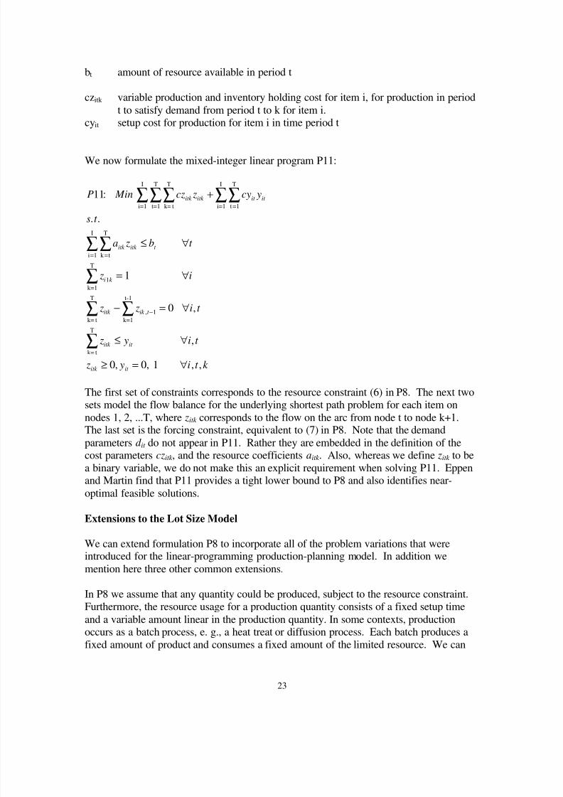
bt amount of resource available in period t

czitk variable production and inventory holding cost for item i, for production in period

t to satisfy demand from period t to k for item i.cyit setup cost for production for item i in time period t

We now formulate the mixed-integer linear program P11:

The first set of constraints corresponds to the resource constraint (6) in P8. The next twosets model the flow balance for the underlying shortest path problem for each item on

nodes 1, 2, ...T, where zitk corresponds to the flow on the arc from node t to node k+1.The last set is the forcing constraint, equivalent to (7) in P8. Note that the demand

parameters d it do not appear in P11. Rather they are embedded in the definition of thecost parameters czitk , and the resource coefficients aitk . Also, whereas we define zitk to be

a binary variable, we do not make this an explicit requirement when solving P11. Eppenand Martin find that P11 provides a tight lower bound to P8 and also identifies near-

optimal feasible solutions.

Extensions to the Lot Size Model

We can extend formulation P8 to incorporate all of the problem variations that were

introduced for the linear-programming production-planning model. In addition wemention here three other common extensions.

In P8 we assume that any quantity could be produced, subject to the resource constraint.Furthermore, the resource usage for a production quantity consists of a fixed setup time

and a variable amount linear in the production quantity. In some contexts, productionoccurs as a batch process, e. g., a heat treat or diffusion process. Each batch produces a

fixed amount of product and consumes a fixed amount of the limited resource. We can

P Min cz z cy y

s t

a z b t

z i

z z i t

z y i t

z y i t k

itk itk it it

itk itk t

i k

itk ik t

itk it

itk it

11

1

0

0 0 1

1

1

:

. .

,

,

, , , ,

,

k= t

T

t=1

T

i=1

I

t=1

T

i=1

I

k t

T

i 1

I

k=1

T

k= t

T

k=1

t-1

k= t

T

∑∑∑ ∑∑

∑∑

∑

∑ ∑

∑

+

≤ ∀

= ∀

− = ∀

≤ ∀

≥ = ∀

==

−



24

model this by introducing an integer decision variable for the number of batches

produced of an item in a time period.

A second variation is when the setups are sequence dependent; that is, the setup for anitem will depend upon what was just previously processed. There is not an easy way to

modify P8 to accommodate this feature. Indeed, in general, the standard representationof sequence-dependent setups is to map this into a traveling salesman problem, which

results in a new level of complexity.

The third variation is when setups can be carried over from one period to the next. In P8we assume that this is not possible; that is, every period that we produce an item we incur

a setup. In some contexts, though, we might be able to preserve the last setup in theperiod. Thus, we would incur only one setup if we produce item i last in one period and

first in the next period. Karmarkar et al. (1987) examine a single-product version of thisproblem. Another variation of this problem is when there are multiple products and we

assume small time buckets, so that at most one item is produced in a period. Lasdon and

Terjung formulate and address this problem by means of column generation. and Eppenand Martin show how to solve both of these problems efficiently by variableredefinition.

Word Count: 7686



25

References

Billington, P. J., J. O. McClain and L. J. Thomas, “Mathematical Approaches to

Capacity-Constrained MRP Systems: Review, Formulation and Problem Reduction,” Management Science, Vol. 29, No. 10 (October 1983), pp.1126-1141.

Bitran, G. R. and D. Tirupati, “Hierarchical Production Planning,” In Handbooks in

Operations Research and Management Science, Volume 4, Logistics of Production and

Inventory, edited by S. C. Graves, A. H. G. Rinnooy Kan and P. H. Zipkin, Amsterdam,

Elsevier Science Publishers B. V., 1993, pp. 523-568.

Bowman, Edward H., “ Production Scheduling by the Transportation Method of LinearProgramming,” Operations Research, Vol. 4, No. 1, (February 1956), pp. 100-103.

Dzielinski, B. P. and R. E. Gomory, “Optimal Programming of Lot Sizes, Inventory and

Labor Allocations,” Management Science, Vol. 11, No. 9 (July 1965), pp. 874-890.

Eppen, G. D. and R. K. Martin, “Solving Multi-Item Capacitated Lot-Sizing ProblemsUsing Variable Redefinition,” Operations Research, Vol. 35, No. 6 (November-

December 1987), pp. 832-848.

Graves, S. C., “A Review of Production Scheduling,” Operations Research, Vol.29, No. 4 (July-August 1981) pp. 646-675.

Hackman, S. T. and R. C. Leachman, “A General Framework for Modeling

Production,” Management Science, Vol. 35, No. 4 (April 1989), pp. 478-495.

Hansmann, F. and S. W. Hess, “A Linear Programming Approach to Production andEmployment Scheduling,” Management Technology, Vol. 1, No. 1, (1960), pp. 46-51.

Hax, A. C. and H. C. Meal, “”Hierarchical Integration of Production Planning and

Scheduling,” In Studies in Management Sciences, Vol. 1: Logistics, edited by M. A.Geisler, New York, Elsevier, 1975, pp. 53-69.

Holt, C. C., F. Modigliani, J. F. Muth and H. A. Simon, Planning Production, Inventories

and Work Force, Englewood Cliffs NJ, Prentice-Hall, 1960.

Karmarkar, U. S., S. Kekre and S. Kekre, “The Dynamic Lotsizing Problem with Startupand Reservation Costs,” Operations Research, Vol. 35, No. 3 (May-June 1987), pp. 389-

398.

Lasdon, L. S. and R. C. Terjung, “An Efficient Algorithm for Multi-Item Scheduling,”Operations Research, Vol. 19, No. 4 (July-August 1971), pp. 946-969.

Magnanti, T. L, J. F. Shapiro, and M. H. Wagner, “Generalized Linear Programming

Solves the Dual,” Management Science, Vol. 22, No. 11 (July 1976), pp. 1195-1203.



Manne, A. S., “Programming of Economic Lot Sizes,” Management Science, Vol. 4, No.2 (January 1958), pp. 115-135.

Shapiro, J. F., “Mathematical Programming Models and Methods for Production

Planning and Scheduling,” In Handbooks in Operations Research and Management Science, Volume 4, Logistics of Production and Inventory, edited by S. C. Graves, A. H.

G. Rinnooy Kan and P. H. Zipkin, Amsterdam, Elsevier Science Publishers B. V., 1993,pp. 371-443.

Silver, E. A., D. F. Pyke, and R. Peterson, Inventory Management and Production

Planning and Scheduling, 3rd

Edition, New York, John Wiley Inc., 1998.

Thomas. L. J. and J. O. McClain, “An Overview of Production Planning,” In Handbooks

in Operations Research and Management Science, Volume 4, Logistics of Production and

Inventory, edited by S. C. Graves, A. H. G. Rinnooy Kan and P. H. Zipkin, Amsterdam,

Elsevier Science Publishers B. V., 1993, pp. 333-370.

Trigeiro, W. W., L. J. Thomas and J. O. McClain, “Capacitated Lot Sizing with Setup

Times,” Management Science, Vol. 35, No. 3 (March 1989), pp. 353–366.

Vollman, T. E., W. L. Berry and D. C. Whybark, Manufacturing Planning and Control

Systems, 3rd

edition, Burr Ridge Ill., Richard D. Irwin Inc., 1992.

Wagner, H. M. and T. Whitin, “Dynamic Version of the Economic Lot Size Model,”

Management Science, Vol. 5, No. 1 (October 1958), pp. 89-96.

Stephen C. Graves

Documents

Transcript of Stephen C. Graves