Stephanie Otema Adu Master Thesis June 6, 2011

i

Title Page

Title: Facies and Petrophysical Analysis and Modelling of

Sandstone Layers: An Evaluation of the Komso Field

Project period: 01-02-11 to 06-06-11

Date of submission: 06-06-11

Place of study: Esbjerg Institute of Technology

Aalborg University Esbjerg

Supervisor(s): Svetlana N. Rudyk

Group member(s): Stephanie Otema Adu

Date: 06-06-11

(Stephanie Otema Adu)

ii

Abstract

The Komso Field located in the West Siberian basin was examined. The purpose of

the project included making zonation, in which reservoir rock was separated from

non-reservoir rock. From the six wells that were analysed, multi-well correlation was

done between them and next, geological analysis was performed in order to identify

the oil and gas-bearing layers. Finally, facies analysis of these layers was done and 3-

dimensional modelling carried out so as to model these characteristics obtained.

Interactive Petrophysics was first used to find these layers. In total, about 25 layers

were found, most of which cut across each of the wells.

Facies analysis1 is important in the investigation of wells and their log information. It

revealed that the predominant facies alternated between transgressive and regressive

bars between the sandstone units. There were some deviations occurring at certain

points, resulting in mouth bars, breaking currents and deltas. Petrel was then used to

obtain facies models as well as models of various petrophysical parameters.

Correlation and modelling was done for layers cutting across the six wells.

Calculations for clay volume, porosity, permeability and water saturation were

performed.

The clay volume found was less than 0.2 over all the layers.

Porosity ranged from 5.9% to 51.6%. Seeing that porosity in general cannot exceed

33.3%, those layers that had higher values are possible overestimations. Permeability

ranged between 1 and 15mD. Most of the layers, for each of the wells, had

hydrocarbon saturations greater than 55%.

The values of the above-calculated parameters suggest that this field is oil-saturated.

Keywords: Reservoir areas, Facies analysis, Clay volume, Porosity, Permeability, Water saturation

iii

Preface

This report has been put together as a final (tenth) semester project report, in partial

fulfillment of the Chemical Engineering (Oil & Gas Technology) MSc. programme

degree at the Aalborg University Esbjerg Institute of Technology. The report explores

sandstone layers of wells of a field, as well as facies analysis. This report may have

specific interest for researchers in the oil and gas industry, such as Schlumberger and

Senergy. It may also be of interest for any companies and industries interested in

facies analysis and modelling.

All references to literature and articles from journals are cited in the references

section at the end of this project report – immediately before the Appendices section.

Reference may also be made to any one of the five appendices found in the report,

especially with respect to charts used for calculations. (For example: [See App. A])

A CD-ROM (attached) contains the entire report.

iv

Acknowledgements

This report is dedicated to the Lord God Almighty who has not only guided me

through this tenth semester project but throughout my whole two-year experience at

Aalborg University. It is also dedicated to my family and friends for all their support.

Special thanks go to my supervisor Svetlana Rudyk who is constantly helpful. She

always gives great advice, not only relating to the project but towards a future career

in petrophysics and life in general.

Many thanks also go to Pawel Spirov & Ismaila Adetunji Jimoh for all their help with

Interactive Petrophysics and Petrel and for always making time for me.

Thanks to Senergy for their provision of the software Interactive Petrophysics, and

Schlumberger, for their provision of the software Petrel. These were both was key in

analysing the wells and evaluating the well log information.

v

Tables & Figures

Tables

Table 1 Dependence of intermediate layer on resistivity ratios ................................. 13

Table 2 Resistivities of various components of reservoir rock .................................. 17

Table 3 Gamma radiation from common minerals and lithologies ........................... 20

Table 4 Common open-hole tools and their uses2 ..................................................... 26

Table 5 Chronostratigraphic and geochronologic unit equivalents ........................... 28

Table 6 Sedimentary Depositional Environment data – Continental ......................... 34

Table 7 Sedimentary Depositional Environment data – Transitional ........................ 36

Table 8 Sedimentary Depositional Environment data – Marine ................................ 38

Table 9 Top and base depths of each layer for each of the six wells ......................... 48

Table 10 Facies analysis for each sandstone unit over the six wells ......................... 57

Table 11 Min, max and reference depth SP values for clay volume calculation ........ 68

Table 12 Clay and sand volumes for each layer of each well.................................... 69

Table 13 Resistivity and salinity information for Well 312R .................................... 76

Table 14 Permeability information for Well 312R ................................................... 77

Table 15 Porosity and water saturation information for Well 312R .......................... 78

Table B 1 Various facies with accompanying vertical, horizontal and SP images ..... 89

Table C 1 Resistivity & Salinity data for Well 335R ................................................ 95





Table D 1 Permeability data for wells 335R, 360R, 333R, 313R and 338R ............ 100

Table E 1 Porosity & Water Saturation data for Well 335R ................................... 102





vi

Figures

Fig. 1 The Reeves 2-arm caliper tool ......................................................................... 2

Fig. 2 An example of an SP log in a sand-shale series ................................................ 5

Fig. 3 Diffusion potential in the lab (a) and in the borehole (b) .................................. 6

Fig. 4 Membrane potential in the lab (a) and in the borehole (b) ................................ 7

Fig. 5 The normal (left) and lateral (right) configurations of the electrical log ........... 9

Fig. 6 The DLL electrode configuration in both the deep and shallow modes .......... 10

Fig. 7 The mode of operation of induction tools....................................................... 11

Fig. 8 Gamma ray values from common lithologies ................................................. 20

Fig. 9 Processes of gamma ray scattering and absorption ......................................... 20

Fig. 10 The neutron logging tool ............................................................................. 22

Fig. 11 Summary of categories and unit-terms in stratigraphic classification ........... 31

Fig. 12 Schematic diagram showing the main depositional environments ................ 33

Fig. 13 An alluvial fan in China’s XinJiang province ............................................... 35

Fig. 14 The shifting nature of the dynamic Mississippi River Delta ......................... 37

Fig. 15 Diagram showing a continental shelf ........................................................... 39

Fig. 16 Components of an oil and gas field .............................................................. 41

Fig. 17 Core sample – sandstone ............................................................................. 46

Fig. 18 Mapping of the six wells for positioning in Petrel........................................ 47

Fig. 19 Initial log plot data for Well 312R ............................................................... 49

Fig. 20 Model of various sandstone layers without and with shale layers ................. 51

Fig. 21 Multi-well correlation generated in Petrel showing various sandstone layers 52

Fig. 22 Top and base contour lines for layers B5, C1, C4, C6 & C7 ......................... 67

Fig. 23 Facies model of all sandstone units across the six wells ............................... 72

Fig. 24 Facies model representation of three layers (layers A5, B5 & C5) ............... 73

Fig. 25 Rweq and Rmfeq determination from Essp ........................................................ 74

Fig. 26 Rweq vs Rw and formation temperature ......................................................... 75

Fig. 27 Salinity determination from Rw and formation temperature .......................... 75

Fig. A 1 Graph for determination of Rmf and Rmc from formation temp. and Rdm ..... 87

Fig. A 2 Graph of microsondes for Rxo determination .............................................. 87

Fig. A 3 Graph of the shallow microlateral log for Rxo determination ...................... 88

Fig. A 4 Graph of microsondes vs shallow microlateral log for Rxo determination ... 88

vii

Contents

Title Page ......................................................................................................................................................................... i

Abstract ........................................................................................................................................................................... ii

Preface ........................................................................................................................................................................... iii

Acknowledgements ................................................................................................................................................... iv

Tables & Figures .......................................................................................................................................................... v

Contents ....................................................................................................................................................................... vii

1 INTRODUCTION ......................................................................................................................... 1

1.1 RESEARCH OBJECTIVE ......................................................................................................................... 1

1.2 PROJECT METHOD ................................................................................................................................ 1

2 WELL LOGGING METHODS ..................................................................................................... 2

2.1 MECHANICAL METHODS ...................................................................................................................... 2

2.1.1 Caliper Logging ............................................................................................................................... 2

2.2 ACOUSTIC LOGGING .............................................................................................................................. 3

2.3 ELECTRICAL METHODS ........................................................................................................................ 4

2.3.1 SP (Spontaneous Potential) Logging ..................................................................................... 4

2.3.1.1 Electrochemical Influence ........................................................................................................................... 5

2.3.1.2 Electrokinetic Influence ............................................................................................................................... 7

2.3.2 Resistivity, Induction Logging................................................................................................... 9

2.3.2.1 Conventional Electrical Logs ...................................................................................................................... 9

2.3.2.2 Dual Laterologs ............................................................................................................................................ 10

2.3.2.3 Induction Logs .............................................................................................................................................. 10

2.3.2.4 Microresistivity Devices ........................................................................................................................... 11

2.3.2.5 Proximity Logs ............................................................................................................................................. 11

2.3.2.6 Resistivity of formation water ................................................................................................................ 13

2.3.2.7 Resistivity of drilling mud ........................................................................................................................ 15

2.3.2.8 Resistivity of mud cakes ........................................................................................................................... 15

2.3.2.9 Resistivity Profile ........................................................................................................................................ 15

2.4 RADIOACTIVE METHODS .................................................................................................................. 18

2.4.1 Natural Gamma Ray Logging ................................................................................................. 19

2.4.2 Neutron Logging ........................................................................................................................... 22

2.4.3 Density Logging ............................................................................................................................. 24

3 STRATIGRAPHY & SEDIMENTOLOGY ...............................................................................27

3.1 STRATIGRAPHY .................................................................................................................................. 27

3.1.1 Absolute & Relative Dating ...................................................................................................... 27

3.1.2 Lithostratigraphy ......................................................................................................................... 28

3.1.3 Chronostratigraphy ..................................................................................................................... 28

3.1.4 Biostratigraphy ............................................................................................................................. 28

3.1.5 Magnetostratigraphy .................................................................................................................. 29

3.1.6 Seismic Stratigraphy ................................................................................................................... 29

3.1.7 Sequence Stratigraphy ............................................................................................................... 30

3.2 SEDIMENTARY DEPOSITIONAL ENVIRONMENTS ........................................................................... 33

3.2.1 Continental (Terrestrial [land])............................................................................................. 34

3.2.1.1 Alluvial fans ................................................................................................................................................... 34

3.2.2 Transitional (Marginal Marine [coastal]) ........................................................................ 36

3.2.2.1 Deltas ............................................................................................................................................................... 36

3.2.3 Marine (Marine [open ocean]) ............................................................................................... 38

3.2.3.1 Continental shelves .................................................................................................................................... 38

4 THE RESERVOIR .......................................................................................................................41

4.1 PERMEABILITY ................................................................................................................................... 41

4.2 POROSITY ............................................................................................................................................ 43

4.3 WATER SATURATION ........................................................................................................................ 44

viii

5 WELL CORRELATION ..............................................................................................................45

5.1 INTRODUCTION .................................................................................................................................. 45

5.2 GEOLOGICAL DESCRIPTION OF THE KOMSO FIELD ...................................................................... 45

5.3 DESCRIPTION OF THE CORE SAMPLE ............................................................................................. 46

5.4 INTERACTIVE PETROPHYSICS .......................................................................................................... 47

5.5 PETREL ................................................................................................................................................ 48

5.5.1 Mapping ............................................................................................................................................ 48

5.5.2 IP Log Data ...................................................................................................................................... 49

5.5.3 Sections .............................................................................................................................................. 49

5.5.4 Horizons ............................................................................................................................................ 50

5.5.5 Models ................................................................................................................................................ 50

6 FACIES ANALYSIS & MODELLING .......................................................................................53

6.1 TYPES ................................................................................................................................................... 53

6.2 MODELLING ........................................................................................................................................ 54

6.3 TRANSGRESSION & REGRESSION .................................................................................................... 55

6.4 SANDSTONE UNITS – KOMSO FIELD ............................................................................................... 57

6.4.1 Description ....................................................................................................................................... 63

6.5 CLAY VOLUME .................................................................................................................................... 68

6.5.1 Sand, Shale distribution of Facies Models ......................................................................... 70

7 CALCULATION OF PETROPHYSICAL PARAMETERS .....................................................74

7.1 FORMATION WATER RESISTIVITY & SALINITY ............................................................................ 74

7.2 PERMEABILITY ................................................................................................................................... 77

7.3 POROSITY & WATER SATURATION ................................................................................................. 77

8 DISCUSSION ...............................................................................................................................79

8.1 FORMATION WATER RESISTIVITY ................................................................................................... 79

8.2 POROSITY ............................................................................................................................................ 79

8.3 PERMEABILITY ................................................................................................................................... 79

8.4 WATER SATURATION ........................................................................................................................ 80

8.5 IP & PETREL ....................................................................................................................................... 80

9 CONCLUSION .............................................................................................................................82

10 REFERENCES ...........................................................................................................................84

11 APPENDICES ...........................................................................................................................87

11.1 APP. A ............................................................................................................................................... 87

11.1.1 Determination of mudcake (Rmc) and mud filtrate (Rmf) resistivity ................... 87

11.1.2 Determination of resistivity of flushed zone, Rxo .......................................................... 87

11.2 APP. B ............................................................................................................................................... 89

11.2.1 Facies ............................................................................................................................................... 89

11.3 APP. C ............................................................................................................................................... 95

11.3.1 Formation Water Resistivity & Salinity data ................................................................ 95

11.4 APP. D ............................................................................................................................................. 100

11.4.1 Permeability data ................................................................................................................... 100

11.5 APP. E ............................................................................................................................................. 102

11.5.1 Porosity & Water Saturation data .................................................................................. 102

1

1 Introduction

1.1 Research Objective This project report seeks to analyse various sandstone layers. A general overview of

the various well logging tools available is given as well as an overview of the

calculations required to determine various parameters. Facies modelling is done in

order to see the distribution of sand and shale throughout each well and the original

setting of the rock present, in which the hydrocarbons are found. Important properties

of an oil and gas field, such as porosity and water saturation, were also determined.

1.2 Project Method Six wells were examined and several Cretaceous sandstone units found for each,

cutting across each well, determining trends between them. Log plot information was

loaded for each using Interactive Petrophysics and modelling for several parameters

was done in Petrel. Various calculations were also performed. Facies analysis helped

to gain a deeper understanding into the original depositional formation of the rock

strata. The overall investigation and interpretation in this research also helped to gain

more knowledge of the Komso field.

2

2 Well Logging Methods

2.1 Mechanical Methods

2.1.1 Caliper Logging

Fig. 1 The Reeves 2-arm caliper tool2

The caliper tool and log is used to determine the shape and size (diameter) of a drilled

hole. It measures variations in the borehole diameter.

There are two main types of caliper log, the independent caliper and the attached

caliper. The first provides detailed information about the conditions of the drilled

hole. It usually has small tips or contact and has a large contact pressure for actual

hole diameter determination.

The second type of caliper is attached to other tools and provides information about

the size of the hole for tool correcting data. It usually has a large contact and operates

under low pressure for the diameter of the fluid column to be found.

As it is being drawn out, after being sent down the borehole, the movement of the

caliper arms is converted into electrical signals by use of a potentiometer.

The caliper tool can have from 2 arms to up to several arms. The choice of which

caliper tool to use depends on the nature of the borehole, as well as how critical the

value must be. The shape of the borehole is not always necessarily perfectly circular.

It may sometimes take on an elliptical shape. In this case, a 2-arm caliper tool would

give an inaccurate value of the borehole diameter, as it would read according to the

longer axis of the oval cross section. If a larger value than expected is obtained, this

suggests that a caliper tool with more arms is required.

3

The caliper log, in addition to providing information on the diameter of the borehole

can also give information on the lithology of the well (if used correctly). If there is a

weak formation, the washouts can provide this data.

It can also give details of fractures, given that if a pair of the caliper arms locks into a

fracture, the tool rotation ceases.1

2.2 Acoustic Logging The acoustic or sonic log measures the travel time of an elastic wave through a

formation. In addition, it can be used to derive the seismic velocity of elastic waves

through this borehole formation. Mainly, it is used in the determination of the porosity

(φ) of a formation by first obtaining seismic data.

The acoustic log has many other uses, including the determination of permeability in

porous rocks and the identification of lithologies, compaction, over-pressures, source

rocks and fractures. The tool works at a higher frequency than seismic waves,

therefore one must be careful with the direct comparison and application of sonic log

data with seismic data. It has both a transmitter and a receiver mounted on it when it

is sent down the borehole. The task is to measure the time taken for either the

compressional (P) wave – which can move through both solids and liquids – or the

shear (S) wave – which can move only through solids – to travel from transmitter to

receiver. The sound waves are generated in all directions by short pulses from the

transmitter.

In order to determine the porosity, the interval transit time must be determined, which

is the recording versus the depth of time taken for a sound wave to move 1 foot

through the formation moving parallel to the borehole wall. It can also be defined as

the slowness of the sound wave. The interval transit time is the reciprocal of the

velocity of the sound wave.2,3

φ = (t – tma)/(tf – tma) or φ = c[(t – tma)/t]

; where t is the reading on the acoustic log

tma is the transit time of the matrix material

tf is the transit time of the saturating fluid

c is a constant with value approximately 0.67.4

4

2.3 Electrical Methods The electrical log is used mainly to determine the water saturation (Sw) from a

formation. From this, the STOIIP (Stock Tank Oil Initially In Place) can be

determined. Since the Sw is derived from the resistivity of the formation water (Rw), it

is extremely important to accurately determine Rw, to get a precise value of Sw in

order to determine the amount of oil in place correctly.

It can also be used to provide information on the lithology, well correlation, and

determination of the shale porosity as well as provide information on source rocks and

recognition of hydrocarbon zones.2

2.3.1 SP (Spontaneous Potential) Logging

This is a tool used to measure naturally distributed charges. Electricity naturally exists

within rock. Two electrodes are placed in the soil, which record the current flow.

The SP can be used to find permeable layers by distinguishing between porous,

permeable reservoir rock and non-permeable shale and clay. It is also used for well

bed correlation, identification of lithologies, as well as providing information on the

shaliness of a formation. It can also be used to confirm the resistivity of drilling mud

and formation water after it has been determined in the lab. This resistivity depends

on temperature, which can eventually be used to determine the water saturation, Sw.4,5

The SP tool consists in general of two electrodes, one within the well and one at the

surface of the well, producing a potential reading without the help of any artificially

applied current flow. It is also referred to as a self-potential. The electrode within the

well is usually made of metal. Ideally it would be made of copper in a

copper(II)sulphate solution in a porous ceramic container. Seeing that these electrodes

are hard to maintain, lead, bronze or stainless steel electrodes are usually used. Some

sources of this spontaneous potential are redox chemical reactions and electrokinetic

fluid flow. The main source is the transport of charged ionic species. This generates

diffusion potentials – a diffusion of ions due to a concentration gradient. This is due

to the fact that positive and negative charges are transported at different rates.

The shale baseline refers to the line in the SP log that can be taken as a static point for

100% shale content, that is, no sand present. It is possible, however, for shale baseline

shifts to occur when there is a difference in salinity between formation waters that are

5

separated by a shale bed that is not a perfect cationic membrane.1,2

Fig. 2 An example of an SP log in a sand-shale series4

In a typical SP log, where the usual case is for the formation water to have a higher

salinity than the mud filtrate, there is a deflection from the shale baseline to the left.

This deflection indicates the presence of sand.4

In order for an SP current to exist:

- the fluid in the borehole must be conductive. This means the drilling mud used

must be water-based.

- there must be a porous and permeable bed found between the low porosity,

impermeable formation

- for the most part, there must be a difference in salinity between the formation

fluid and the borehole fluid. The SP current may however arise due to difference

in fluid pressure instead.2

There are two main sources of spontaneous potential (current):

2.3.1.1 Electrochemical Influence

Diffusion potential/liquid junction potential – This refers to the spontaneous potential

found at the junction between the invaded and uninvaded zones and is an

electromotive force. It arises due to the difference in salinity between the formation

fluid and the borehole fluid, which in this case is the mud filtrate.

6

(a) (b) Fig. 3 Diffusion potential in the lab (a) and in the borehole (b)

2

Assuming NaCl to be the only source of salinity and the salinity of the formation fluid

to be higher than that of the borehole fluid, there is a net movement of negative

charge from the uninvaded to the invaded zone – diffusion. This is because the ions

move from an area of higher salinity to a lower salinity area and also because the Cl–

ions are smaller and therefore more mobile than the Na+ ions. This sets up an SP

current, due to the charge imbalance, flowing from the invaded to the invaded zone.2

Ed = –11.81*log(R1/R2)

; where Ed is the diffusion potential

R1 is the resistivity of the less saline solution

R2 is the resistivity of the more saline solution

Also, Ec = –K*log(aw/amf)

; where Ec is the total electromotive force

K is a co-efficient that is proportional to the absolute temperature. Its value is

71 at 25oC [K = 65 + 0.24T(

oC)]

a is the chemical activity at formation temperature (of either the formation

water or mud filtrate)

Shale/membrane potential – This is the SP found at the junction of the uninvaded and

shale zones. Shale has a property of being anionically or electronegatively

permselective. They retard the movement of anions – due to the presence of an

electrical double layer. This leaves the shale preferentially positive, setting up a

potential between the shale and uninvaded zones. This results in a current flow from

the uninvaded zone of the formation to the shale zone, and eventually into the

borehole.2

7

(a) (b) Fig. 4 Membrane potential in the lab (a) and in the borehole (b)

2

2.3.1.2 Electrokinetic Influence

Mudcake potential – This is the SP produced by the movement of charged ions

through the mudcake and the invaded zones of a permeable formation. Since the

mudcake is of low permeability, this is usually as far as the SP gets, hardly ever

reaching the invaded zone.

Mudcake, like shale, also has the property of anionic permselectivity. There is

therefore a net current flow from the borehole to the mudcake.

Shale wall potential – this arises from the flow of fluid from the borehole to the shale

zone. It is usually a small value seeing that the shale is impermeable and fluid flow

into it is highly limited.

The Static spontaneous potential (SSP) refers to the total voltage obtained from the

diffusion of ions across the liquid and membrane junctions. This arises due to the fact

that there is now mud filtrate in the well formation that was not there at the time the

well was drilled. This value decreases as the contrast in resistivity between the

formation water and the mud filtrate decreases. It also switches sign if the resistivity

of formation water is found to be higher than the resistivity of the mud filtrate.2

The SSP opposite a permeable bed is found if the current is prevented from flowing,

which may be due to the presence of strong insulators, such as insulating plugs.

SP current flows through the borehole, the invaded zone, the uninvaded zone and the

surrounding shale, with the largest fraction of the current – and therefore the largest

SP deflection – travelling through the borehole. Because of this, there is a very large

potential drop, seeing that the borehole’s cross-sectional area is relatively small as

compared with the formation and its resistance would therefore be high.

8

The total potential drop in this case would therefore be the total electromotive force,

the SP deflection ideally opposite a thick, clean formation. In this case there is a lower

resistance and the SP would be very close to the actual SSP. Shaliness in the bed is

ignored in this case, as well as other sources of potential. It is also assumed that the

shale is a membrane that is perfectly cationic.4,6

Its value can be determined directly from the SP curve as the difference between the

SP maxima opposite the permeable bed and the shale baseline. This can be done as

long as the bed is porous, permeable, non-shaly, clean, thick, has saline formation

water, drilling mud that is not too resistive and moderate invasion. If the beds meet all

these requirements but are thin, corrections can be made for bed thickness using

correction charts.

A clean, non-shaly bed is required in order to accurately obtain the resistivity of the

formation water, Rw from SP.

In cases where different salts other than NaCl predominate or are found, it affects the

value of the SSP. This needs to be taken into consideration. CaCl2 and MgCl2 are the

usual salts that are found in addition to NaCl. The SSP is therefore:

SSP = –K*log [aNa + (aCa + aMg)1/2

]w / [aNa + (aCa + aMg)1/2

]mf

The ionic activities of Na, Ca and Mg, knowing their concentrations, are found from a

chart. It is important to find the respective K values where other salts predominate.

Several assumptions are made for SP including the ionic activity being inversely

proportional to the resistivity. Another assumption is that the mud filtrate and

formation water have properties of an ideal sodium chloride solution.

For conditions that do not conform to these assumptions, the equivalent resistivity and

ionic activity are introduced. This would be for cases where the concentration of the

NaCl solution is very high.

Rweq = A/aw

; where Rweq ≡ equivalent resistivity of formation water

aw ≡ activity of formation water

A ≡ constant chosen so that Rw = Rweq in dilute solutions

The static SP can then be determined using these equivalent resistivities:

SSP = –K(T)log(Rmfeq/Rweq)

9

2.3.2 Resistivity, Induction Logging

The resistivity of fluids within a well refers to the amount of electrical resistance the

fluid has to the passage of current through it. It is said to be the reciprocal of

conductivity and is measured as:

Resistivity = (Resistance * Area)/Length; R = (r*A)/L

Its unit is the ohm-m. (ohm-meter or Ω-m)

Sedimentary formations are capable of transmitting an electric current only by means

of the interstitial and adsorbed water they contain, and if entirely dry would be non-

conductive. The electrical resistivity of a fluid-saturated rock is its ability to impede

the flow of electric current through that rock. Dry rocks exhibit infinite resistivity.

The resistivity log is extremely important in the characterisation and evaluation of an

oil & gas field because it is the only reliable method for hydrocarbon detection.

The neutron log method can also be used, however, this method is based on a

hydrogen index and the values for oil and water are very close. The value for gas is

quite different though and hence the neutron method is useful for gas detection.

There are several different logs that constitute the resistivity log, each having their

specific method of determining resistivity and their own corrections.2

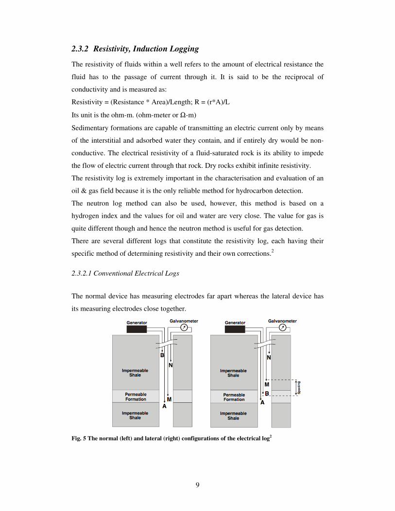
2.3.2.1 Conventional Electrical Logs

The normal device has measuring electrodes far apart whereas the lateral device has

its measuring electrodes close together.

Fig. 5 The normal (left) and lateral (right) configurations of the electrical log2

10

2.3.2.2 Dual Laterologs

This is made up of two tools, one run in deep penetration and the other in shallow

penetration.

Fig. 6 The DLL electrode configuration in both the deep (LLd) and shallow (LLs) modes

2

2.3.2.3 Induction Logs

These were initially made for oil-based drilling muds but can now be used in high

salinity water-based or fresh water-based drilling muds.

The sonde is made up of a transmitter, a receiver and two wire coils. An alternating

magnetic field around the sonde arises due to the high frequency alternating current

applied to the transmitter. This induces a secondary current and consequently an

alternating magnetic field in the formation, which in turn induces current in the

receiver of the sonde. The signal is measured and is proportional to the conductivity

of the formation. An induction log’s peaks therefore always deflect in an opposite

direction to the resistivity curves.

The induction log is usually coupled with the SP log in the same track of the log plot.

This gives an idea of hydrocarbon presence in a layer. If their deflections are in the

same direction, this is an indication of the presence of oil, whereas if their deflections

are in opposite directions, this suggests the presence of water.

11

Fig. 7 The mode of operation of induction tools

2

2.3.2.4 Microresistivity Devices

These have similar electrode setups as the modern resistivity logs, but the electrode

spacings are much smaller – only a few inches. The penetration of these tools is

therefore only to a small degree and usually does not even go through the mudcake.

The sonde of these devices is pressed against the borehole wall.

Microlog – this additionally provides extra caliper readings, known as the

microcaliper log.

Microlaterolog – this is a micro scale version of the laterolog.

Proximity log – this is focused only a short distance from the formation. It is larger

than the microlaterolog and is an improvement of it, dealing with issues of mudcakes

thicker than 3/8 of an inch. It therefore has minimal influence from the mudcake or, in

ideal cases, the undisturbed zone. It measures the resistivity of the flushed zone, Rxo.

Microspherically focused log – this is usually run together with the dual laterolog. It

also measures Rxo. The resistivity is considered to be most accurately calculated when

the current flows spherically around the current-emitting electrode.2,4

2.3.2.5 Proximity Logs

The proximity log (referred to as microsondes here) is used together with the shallow

microlateral log to determine the resistivity of the flushed zone [area completely taken

over by drilling mud or mud filtrate]. This is why only the shallow microlateral log is

considered, since the deep microlateral log has not yet been affected by the drilling

mud to affect this measurement.

This determination can be done in several combinations:

Microlateral microsonde vs. Micronormal microsonde [Figure A2, App. A]

12

From the logging plot, the apparent resistivity, Rapp, for each microsonde is found.

This is divided by the resistivity of the mudcake, Rmc.

The resistivity of the drilling mud, Rm, is typically given from a measurement done at

the well site. The resistivity of the mud filtrate, Rmf, and the resistivity of the

mudcake, Rmc, can be found from a chart [Figure A1, App. A]. In general, the

relationship Rmf = 0.8Rm can be used to determine the resistivity of the mud filtrate.

The Rapp/Rmc values for both microsondes are read off on the microlateral versus

micronormal graph.

It is ensured that this intersection matches with the height of the intermediate layer, l

(in mm) ‘l’ is measured as the distance between the borehole wall and the well

logging tool. It can sometimes be referred to as the thickness of the mudcake, hmc.

l = [dbit – dcaliper]/2

The corresponding value for Rxo/Rmc, is read off the graph and the flushed zone

resistivity, Rxo, is determined.

Microlateral [shallow] [Figure A3, App. A]

From the logging plot, the apparent resistivity, Rapp, is determined. It must be noted

that the plot is in logarithmic scale and must be measured accordingly.

The apparent resistivity is divided by the resistivity of the mudcake, Rmc

The intersection of the Rapp/Rmc value and the height of the intermediate layer, l, is

found.

From this intersection, the corresponding value for Rxo/Rmc is determined and the

flushed zone resistivity, Rxo, calculated.

Microsondes vs. Microlateral [shallow] [Figure A4, App. A]

From the logging plot, the apparent resistivity, Rapp, for each microsonde is found as

well as Rapp for the shallow microlateral log.

The values for Rapp/Rmc are found for each.

The intersection of the Rapp/Rmc value for each microsonde (separately) with the

Rapp/Rmc value for the shallow microlateral is found.

This intersection for each is matched with the height of the intermediate later, l, the

corresponding Rxo/Rmc value found and the flushed zone resistivity, Rxo, determined.

There are, however, some limitations to applying this method:

The height of the intermediate layer, l, must be less than 15mm (l<15mm) in order for

13

the resistivity (of the flushed zone) read to be accurate. If l>15mm, then the

dependence is on resistivity ratios.7

Table 1 Dependence of intermediate layer on resistivity ratios

l, mm 10 15 20 30

Rxo/Re 1 – 1500 1 – 250 1 – 100 1 – 35

; where Re is the resistivity of the intermediate layer area.

The thickness of the mudcake should be less than 15mm. If the thickness exceeds this,

the intermediate layer would not be able to be used for quantitative interpretation.

High distortions of the resistivity values occur when the resistivity of the drilling mud

is low. Distortions occur when Rm < 0.50ohm-m.

2.3.2.6 Resistivity of formation water

Formation water, also known as interstitial water, is that which occurs naturally

within the rock pores. It is found in the undisturbed zones surrounding the wellbore.

Drilling mud and other fluids injected or introduced into the borehole during

production do not constitute formation water.

Its resistivity, as well as other properties, can be used for interpretations of

measurements made within the well and on the surface.4,6

The resistivity of formation water, Rw, is most commonly calculated from the SP log:

The standard SP response equation can be expressed as:

SSP= -Kc * log[Rmfeq/Rweq] (1)

Re-arranging Equation 1 and solving for Rweq ;

Rweq=[Rmfeq/(10(SSP/-Kc))]

; where

SSP is Static SP (mV) measured from a shale baseline,

Rmfeq is equivalent resistivity of mud filtrate at formation

temperature,

Rweq is equivalent resistivity of formation water,

Kc = 61+ .123*T(oF) or,

Kc = 65+ .24*T(oC)

Analysis Procedure

The SP deflection from the shale baseline, preferably from a thick, clean water sand,

is measured. If the mud filtrate resistivity (Rmf ) at 75oF is higher than 0.1, Rmf is

14

corrected to the formation temperature using:

Rmf = [Rmf at surface temp * (Surface temp + 6.77) ]/ (Bottom hole temp + 6.77)

The Schlumberger General Chart can also be used with Rmfeq = 0.85Rmf.

If Rmf at 75oF is lower than 0.1, Rmf is corrected to formation temperature and a chart,

such as Schlumberger's Sp-2, used.

Equation (1) is used to calculate Rweq.

Formation water resistivity (Rw) is estimated using Chart SP-2.

Water salinity is estimated using a Schlumberger general chart [see Fig. 27] 10

Rw can also be obtained from resistivity ratios:9

(1)

(2)

F is Formation Factor

Rw is the resistivity of the formation water

Ro is the resistivity of a reservoir rock fully saturated with

brine,

Rmf is the resistivity of the mud filtrate

Rxo is the resistivity of the filtrate saturated reservoir

Combining and rearranging equations (1) and (2), Rw can be solved for:

Both Ro and Rxo measurements must be corrected for borehole environmental effects using

appropriate service company charts. Rmf is corrected to formation temperature using;

for Fahrenheit, or,

for Celsius.

T 1 is the mud filtrate surface temperature read from the

log header,

R1 is the measured mud filtrate resistivity from the log

header,

15

T2 is formation temperature,

R2 is mud filtrate resistivity at formation temperature.

2.3.2.7 Resistivity of drilling mud

Also referred to as drilling fluid, drilling mud refers to the fluid that is used in

hydrocarbon drilling operations. These drilling muds can be water-, oil-, gaseous-, or

synthetic-based. They typically contain large amounts of suspended solids as well as

emulsified oils and water. It is injected into a drilled borehole’s injection well with the

aim of displacing hydrocarbons found in porous space towards the production wells.

Rm, as mentioned above, is usually obtained from measurements done at the well

site.6

2.3.2.8 Resistivity of mud cakes

Once drilling fluid has been injected into the injection wells of a drilled borehole, it

forces its way, under pressure, through the permeable parts of the reservoir. This

leaves behind a residue, which is deposited on the borehole wall and is known as the

mudcake. The liquid that passes through the permeable area is known as the mud

filtrate. Mudcake properties such as its thickness, toughness, slickness

and permeability are important because the mudcake that forms on permeable zones

in the wellbore can cause a choked pipe amongst other drilling problems. Reduced oil

and gas production can result from reservoir damage when a poor filter cake allows

deep filtrate invasion. A certain degree of cake buildup is desirable to isolate

formations from drilling fluids. In open-hole completions in high-angle or horizontal

holes, the formation of an external filter cake is preferable to a cake that forms partly

inside the formation. The latter has a higher potential for formation damage.

The resistivity of the mudcake, Rmc is found from Rm and the formation temperature.6

(10,11,12,13,14) [see Figure A 1, App. A]

2.3.2.9 Resistivity Profile

This is based on drilling mud that has a fresh water base and is formed from the

flushed zone through the invaded zone to the uninvaded zone (from shallow to deep).

Flushed zone: this is the shallow part of the well. This zone has been completely

overcome by drilling mud filtrate. It is made up of this drilling mud filtrate and rock.

Invaded zone: This is a type of transition zone and is made up of a mixture of rock,

drilling mud as well as oil, gas or water.

16

Uninvaded zone: as the name suggests, this is the zone where no drilling mud has yet

infiltrated. This zone may be made up of a mixture of rock, oil, gas and water in

various combinations. This is the deep part of the well.

Measurements are usually done for just the shallow and deep parts of the well. These

would give more accurate values for resistivity than the invaded zone, since it is much

harder to determine the amount of drilling mud in this zone.

Different resistivity profiles are obtained for zones primarily containing oil and those

containing water.

For oil:

Drilling mud has a higher conductivity than oil, implying that it has a lower

resistivity. Therefore, in the flushed zone, where only drilling mud filtrate is found,

there would be a low resistivity. In the invaded zone, where there is a decrease in the

amount of mud filtrate and increased amounts of oil, the resistivity gradually

increases. In the uninvaded zone, where no drilling mud is found, there is only oil and

therefore high values for the resistivity. This is shown in the resistivity profile above.

For water:

Drilling mud has a lower conductivity than water, implying that it has a higher

resistivity. In the flushed zone, there is high resistivity. In the invaded zone, where

there is a decrease in the amount of mud filtrate and increased amounts of water, the

resistivity gradually decreases. In the uninvaded zone, with no drilling mud and only

water, there are low values for the resistivity, as seen in the resistivity profile above.

flushed invaded uninvaded

flushed invaded uninvaded

17

The Archie equations are of extreme importance for the resistivity log. They provide a

relationship between the resistivity of the formation and the resistivity of the fluids

saturating the formation.

Conductivity and resistivity are inversely proportional:

C(mS/m) = 1000/R(ohm–m)

Reservoir rocks can be made up of the following with their respective resistivity.

Table 2 Resistivities of various components of reservoir rock2

Matrix material High resistivity

Oil High resistivity

Gas High resistivity

Formation water Low resistivity

Water-based mud filtrate Low resistivity

Oil-based mud filtrate High resistivity

In the uninvaded zone of a formation, the resistivity of the formation depends on the

amounts and resistivities of the formation fluids. The rock in this formation comprises

oil, gas and formation water.

The resistivity of a formation in the uninvaded zone depends on the porosity, the

resistivity of the formation water and the water saturation. It is known as the true

resistivity and can only be calculated using deeply penetrating electrical logging tools.

The invaded zone has been (partially) overcome by drilling fluid. The resistivity of

the formation in this zone depends on the porosity, the saturation and resistivity of the

mud filtrate and the saturation and resistivity of the formation water if present.

The bulk resistivity of rock, Ro, is directly proportional to the fluid resistivity, Rw,

when the rock is fully saturated with this aqueous fluid.

The constant of proportionality here is the formation factor and arises due to the effect

of the presence of the rock matrix.

The formation factor, F, is 1 where there is no rock matrix and is greater than 1 in

porous media such as rock.

Ro = F*Rw

Relating the formation factor to the porosity, it is found that:

F = φ–m

; which is Archie’s first law.

Substituting the second equation into the first:

Ro = Rwφ–m

; where m is the cementation factor and describes the increase in resistivity due to the

presence of insulating mineral grains (rock) that force the current to take a winding

18

path through the conducting fluid. This value usually ranges between 1 and 3.

If however, there is only partial water saturation of the rock, then the bulk resistivity

of the rock, Rt, partially saturated with aqueous fluid of resistivity Rw, is directly

proportional to the resistivity of the rock fully saturated with the same fluid. This

partial water saturation gives:

Rt = I*Ro

; where I is the resistivity index and arises due to the effect of partial desaturation of

the rock. Fully saturated rock has I=1 and rock that is full of dry air has I approaching

infinity (∞).

Relating the resistivity index to the fractional water saturation of the rock:

I = Sw–n

Substituting the second equation into the first:

Rt = Ro*Sw–n

; where n is the saturation exponent and ranges usually between 1.8 and 2. This value

is determined from lab experiments on core samples.

Combining both laws and rearranging for Sw determination:

Sw = n[(Rwφ–m

/Rt)1/2

] = n[(RwF/Rt)1/2

] = n[(Ro/Rt)1/2

]

The saturation of the mud filtrate, Sxo = n[(Rxo,mf/Rxo,or)1/2

];

; where Rxo,mf is the resistivity of the flushed zone that is 100% filled with mud filtrate

Rxo,or is the resistivity of the flushed zone containing residual oil

The saturation of the mobile oil is therefore found to be Sxo – Sw.

The volume of the mobile oil per unit volume of the rock is φ(Sxo – Sw).

2.4 Radioactive Methods The radioactivity log, also known as the nuclear or radiation log records the natural or

induced radioactive properties of wellbore formations. It is typically made up of the

gamma ray and neutron logs. Below, the density log is also discussed. These logs help

in the determination of the type of rock formation and the nature of the fluid found in

these rocks.6

All atoms consist of a nucleus, containing a certain number of uncharged neutrons

and a fixed number of positively charged protons. Some atoms have varying neutron

numbers, which leads to the existence of different isotopes of atoms.

Surrounding the nucleus are negatively charged electrons. There are the same number

of electrons and protons in a neutral atom.

19

If an isotope is considered unstable, with high energy, there are several ways it can

release this energy to become stable. One such method is through the emission of

gamma rays, which have no mass and no charge, a process of spontaneous decay.

The gamma ray log measures the natural radiation from a formation whereas the

neutron and density logs measure the radiation generated by the particular tool used.2

2.4.1 Natural Gamma Ray Logging

Gamma ray logging can be divided into total and spectral gamma ray logs. The total

gamma ray log measures the total natural radiation from a formation with the use of a

gamma ray detector. Its use is mainly for the determination of the lithology of the

formation, shale content and depth matching. The spectral gamma ray log measures

the natural radiation from a formation separated into its contribution from each

gamma-emitting source. It is also used in the determination of the lithology as well as

in uncertainty detection and inter-well correlation.

The gamma ray penetrations are the highest of all radiations, with the exception of

neutrons. The most important isotopes that involve gamma ray emission can be found

in gamma ray emitting sources. These are the potassium (K) isotope, the Thorium

(Th) series isotopes and the Uranium-Radium (U-Ra) series isotopes.

Potassium gives a distinct peak at 1.46MeV and has the highest radioactivity

recording, followed by shales.

Shale is the lithology that most commonly emits gamma rays. It is made up of

igneous rock, containing feldspars and micas, which are gamma ray emitting sources.2

20

Table 3 Gamma radiation from common minerals and lithologies2

Fig. 8 Gamma ray values from common lithologies

2

The gamma rays that are emitted can undergo different processes depending upon the

amount of energy they have.

Fig. 9 Processes of gamma ray scattering and absorption

2

21

From Fig. 9 it can be seen that:

- If the amount of energy exceeds 3MeV, the gamma rays collide with the nucleus of

the atom of the material through which they are passing, resulting in pair production –

the conversion of the gamma rays to an electron and a positron.

- If the amount of energy lies between 0.5MeV and 3MeV, the gamma rays collide

with the atom of the material through which they are passing and eject an electron

from the atom. The gamma rays, in turn, lose energy. This is known as Compton

scattering.

- If the amount of energy is less than 0.5MeV, the gamma rays collide with the atom

of the material through which they are passing and are absorbed. The energy from the

gamma rays is then used to eject an electron or promote it to a higher energy level.

This is known as photoelectric absorption.

Therefore, step 2 occurs until the energy is low enough for step 3 to occur.

The density of the material through which the gamma ray is traveling – whether the

formation, the fluids, the mudcake or the drilling mud – affects the count rate. The

higher the density, the more attenuation will occur and the lower the signal will be,

and vice versa. This is sorted by the borehole correction.

The GR log is particularly useful for defining shale beds when the SP is distorted (in

very resistive formations), when the SP is featureless (in freshwater-bearing

formations or in salty mud; i.e., when Rmf Rw), or when the SP cannot be recorded

(in nonconductive mud, empty or air-drilled holes or cased holes). The bed boundary

is picked at a point midway between the maximum and minimum deflection of the

anomaly.4

22

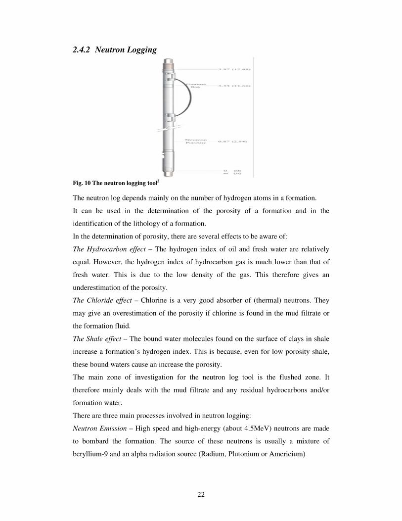
2.4.2 Neutron Logging

Fig. 10 The neutron logging tool2

The neutron log depends mainly on the number of hydrogen atoms in a formation.

It can be used in the determination of the porosity of a formation and in the

identification of the lithology of a formation.

In the determination of porosity, there are several effects to be aware of:

The Hydrocarbon effect – The hydrogen index of oil and fresh water are relatively

equal. However, the hydrogen index of hydrocarbon gas is much lower than that of

fresh water. This is due to the low density of the gas. This therefore gives an

underestimation of the porosity.

The Chloride effect – Chlorine is a very good absorber of (thermal) neutrons. They

may give an overestimation of the porosity if chlorine is found in the mud filtrate or

the formation fluid.

The Shale effect – The bound water molecules found on the surface of clays in shale

increase a formation’s hydrogen index. This is because, even for low porosity shale,

these bound waters cause an increase the porosity.

The main zone of investigation for the neutron log tool is the flushed zone. It

therefore mainly deals with the mud filtrate and any residual hydrocarbons and/or

formation water.

There are three main processes involved in neutron logging:

Neutron Emission – High speed and high-energy (about 4.5MeV) neutrons are made

to bombard the formation. The source of these neutrons is usually a mixture of

beryllium-9 and an alpha radiation source (Radium, Plutonium or Americium)

23

The equation above shows that fast neutron Carbon-12 and gamma rays are produced.

Neutron Scattering – Elastic scattering occurs due to the collision of these fast

neutrons with the nucleus of the atom in the formation. Since the size of the neutron

and the hydrogen atom are similar, the most effective scattering (resulting in a loss of

energy of the neutron) occurs between these two, and less efficiently for larger atoms.

The high-energy neutrons lose energy and become low energy neutrons or high-

energy gamma rays.

Neutron Absorption – Eventually, after several collisions, the lowest energy thermal

neutrons are absorbed by the nucleus of the atom of the formation. Hydrogen and

chlorine are two elements with relatively high neutron absorbing characteristics. The

effectiveness of neutron absorption depends on the element involved.

The partial concentration of hydrogen per unit mass can be defined as:

(mass of hydrogen atoms in the material) / (mass of all elements in the material)

Hence, the partial conc. of hydrogen per unit vol = (partial conc./unit mass) * density

The Hydrogen Index can be defined as the partial concentration of hydrogen per unit

volume relative to water.

When the Hydrogen index = 1, it implies that the porosity = 1

Types of Neutron Logging Tool

Gamma Ray/Neutron Tool

This has a neutron source and a single detector. It can be used in open or closed holes

and the tool is centered within the borehole. It is sensitive to borehole conditions such

as borehole quality, temperature, drilling mud type and mudcake thickness. It is also

sensitive to thermal neutrons and therefore also sensitive to hydrogen and chlorine.

Correction curves therefore exist to account for these effects.

Sidewall Neutron Porosity Tool

This also has a neutron source and a single detector. It can, however, only be used in

open holes and the tool is pressed against the borehole wall. It is not affected by

drilling mud. Neither is it affected by chlorine or hydrogen since it is only sensitive to

epithermal neutrons. These have higher energy and are not yet at the stage for

absorption by elements.

Compensated Neutron Log

This is made up of a neutron source and two detectors and is pressed up against the

24

borehole wall. It is sensitive to thermal neutrons and therefore also chlorine and

hydrogen. The larger detector is found close to the source to ensure an accurate count

rate. The two detectors help to compensate for the chloride effect – from chloride-rich

mudcake and mud filtrate.

The neutron log, in responding to the presence of these hydrogen atoms, deals mainly

with liquid-filled pore space of the formation, where the response is generally a

measure of the porosity, φ.

2.4.3 Density Logging

The formation density log measures the bulk density of a formation. This is done in

order to determine the total porosity. It is also used to detect gas-bearing formations

and evaporates.

The density logging tool is made up of:

- a radioactive source of either Cs-137 or Co-60 which releases gamma rays with

energy ranging from 0.2-2MeV.

- a short range detector which is found closer to the source

- a long range detector

There are two detectors to help correct for the effects of the mudcake.

The gamma rays released from the source undergo Compton scattering in which the

energy of the rays reduces in a stepwise fashion and the rays are scattered in all

directions. The collisions occurring depend on the number of electrons in the

formation.

Once the energy is low enough, ie. below 0.5MeV, photoelectric absorption occurs

upon collision with atomic electrons.

A high bulk density means a high number density of electrons, which indicates a high

attenuation of the gamma rays and a low count rate of these gamma rays recorded by

the detectors. The vice versa conditions also apply.

A high-density mud affects the readings of the detector. This is because as stated

before high density leads to high rates of absorption of the gamma rays. These effects

are accounted for by the spine and rib corrections.

There are many uses of the density log in addition to the main ones mentioned above.

It can also be used to identify the lithology and detect fractures as well as shale

compaction, age and unconformities in the formation. It is used in the identification

25

of minerals in evaporite deposits, for gas detection as well as hydrocarbon density

determination.2

The density tool, in responding to the electron density [number of electrons per cubic

centimetre of formation] of the particular material in the formation, can determine the

porosity from the bulk density:

φ = (ρma – ρb)/ (ρma – ρf)

; where ρma is the density of the formation or rock matrix

ρb is the bulk density

ρf is the density of the pore fluid1,4

26

Table 4 Common open-hole tools and their uses2

27

3 Stratigraphy & Sedimentology

3.1 Stratigraphy

Stratigraphy refers to the study of strata or layers. It deals with the analysis of rock

successions over time and through changing environments.

There are three main types of rocks – sedimentary, igneous and metamorphic rocks.

Seeing that sedimentary rocks follow a more predictable pattern, stratigraphy is

usually associated with this type of rock. Deposition of igneous and metamorphic

rock is less predictable and hence is hardly used.

This is of much use in the oil and natural gas or petroleum industry seeing that the

majority of oil and gas reserves for the most part occur in stratified sedimentary rocks.

It is therefore advantageous to know which type of rocks to focus on.15

Stratigraphic signatures and stratal patterns in sedimentary rock record are a result of

the interaction between tectonic activity, eustasy and climate.

The effect of tectonics and eustasy is that they determine the available space that will

be filled with sediment. The three together control the sediment supply and determine

actually how much of this available space will be filled.16

3.1.1 Absolute & Relative Dating

Absolute Dating is also referred to as chronometric or calendar dating. This form of

dating seeks to determine an approximate computed age of rock strata: Radiometric

Dating [Radiocarbon dating, Potassium-Argon dating], Thermoluminescence dating.

Chronostratigraphy, defined below, deals with the absolute dating of rock strata.

Relative Dating, also known as internal industry, does not find an approximate age,

but determines the relative order and sequence in which certain events took place.

Biostratigraphy, described more below, stems from this. The Law of Superposition, as

well as the Law of Faunal Succession, also explained below, was derived from, and

sums up, the theory of relative dating.

Different types of rocks repeat themselves over time. It is, therefore, usually very hard

to determine the exact age of rocks. Analysis of the fossils that make up these rocks,

however, can help with this.

28

There are many types of stratigraphy studied today. The more classical forms of

stratigraphy are:

3.1.2 Lithostratigraphy

This refers to the study and correlation of strata to determine information about the

Earth’s history. The information is based on their lithology, or the nature of the well

log response, mineral content, grain size, texture and color of rocks.6 It is the

characterisation of rock strata by the kind and/or arrangement of their mineralogical

constituents. Therefore, it is the physical characteristics of the layered rock strata that

are studied. Similar lithologies are usually diachronous and therefore have no time

significance. Some uses of lithostratigraphy, however, include placing specific

geological units in a particular geologic framework, establishing a stratigraphic

relationship with geological units above and below and aiding in the correlation

between other lithologic units.15

3.1.3 Chronostratigraphy

This can be referred to as the characterisation of rock strata based on their temporal

relations. It seeks to find the ages of rocks based on when they were formed.

Chronostratigraphic units are bodies of rock that were formed within a specific

geological period of time. It is the basis for the time scale of the Phanerozoic eon.

Chronostratigraphic units are very closely linked to geochronological units, though

the latter units represent the actual interval of time. Chronostratigraphic units measure

how much sediment was deposited in that time and cannot be defined as actual time.

The table below shows the geochronological and chronostratigraphic unit

equivalents.15,17

Table 5 Chronostratigraphic and geochronologic unit equivalents with an example15

3.1.4 Biostratigraphy

This deals with the study of the temporal and spatial distribution of fossil organisms.

The correlation and dating of rocks is usually found through this method, and may be

done on a global scale, between basins, within a basin or within an oil field.

29

Therefore, once two particular types of rock made up of the same fossils, regardless

of their location at the present time and though sedimentary rock changes over time,

they can be thought to have been deposited or formed at the same time. There are

many different types of fossil assemblages that are used in this type of stratigraphy.

Some of them include ammonites, index fossils and trilobites and some microfossils

such as chitinozoans, foraminiferans, pollen and spores.18

3.1.5 Magnetostratigraphy

Magnetostratigraphy gives relatively precise chronology in strata independent of

fossil content. This type of stratigraphy correlates magnetic reversals found in a

stratigraphic column with reversal ages derived from sea-floor magnetihc stripes.

Magnetostratigraphic geochronometry works best in fine-grained neogene,

siliciclastic strata, but it can be used effectively in rocks as old as Middle Jurassic. In

rocks that predate the oldest modern sea-floor, magnetic reversal patterns can still be

used as correlative tools.

Natural Remanent Magnetisation (NRM) is the basis of magnetostratigraphy. It

represents a rock or sediment’s permanent magnetism. It can also preserve a record of

the Earth’s field and the tectonic movement of the rock or sediment for millions of

years.19

3.1.6 Seismic Stratigraphy

This process seeks to utilise seismic data in the interpretation of stratigraphic

information. Though there may be some exceptions, it is generally accepted that

within the resolution of the seismic method, the seismic reflections follow gross

bedding, and can be considered as timelines. These timelines represent time surfaces

in three-dimensional space and can separate and distinguish older rocks from younger

ones. Seismic stratigraphy helps give chronostratigraphic as well as lithostratigraphic

information from the reflection characteristics at impedance contrasts.16

Where there is a difference in density or velocity between physical structures, seismic

reflections are generated. They follow stratal surfaces or bedding planes, and not

gross lithostratigraphic boundaries, and these stratal surfaces separate the various

processes of sedimentation. Together with unconformities, they are the two interfaces

that are generated at the time of deposition in a sedimentary section. Changes in the

deposition that may have occurred in a basin, and subsequent geological subdivision

into stratal units or depositional sequences, can be found through this method,

30

together with the law of superposition. This is done through the recognition of

unconformity surfaces. Unconformities, though they do not directly provide

chronostratigraphic information, always have younger rock or strata above and older

rock below. There are several other useful features of seismic stratigraphy. The

seismic reflections are helpful in paleogeology reconstruction, and from that, also

paleogeography and paleoenvironmental reconstruction, which seeks to reconstruct

the initial and original conditions of the environment. Once depositional units have

been determined, an estimation of the reservoir rock content can be done, as well as

facies predictions made. It is also very useful as a chronostratigraphic tool, in addition

to finding stratigraphic traps.20

A more integrated form of stratigraphy, which incorporates several aspects of the

aforementioned types of stratigraphy, is:

3.1.7 Sequence Stratigraphy

This stems mainly, however, from seismic stratigraphy. This type of stratigraphy

subdivides sedimentary basin fills into genetic packages bounded by unconformties

and correlative conformities. It can therefore provide correlation and mapping of

sedimentary facies and stratigraphic prediction from a chronostratigraphic framework.

It is the analysis of genetically related depositional units within a chronostratigraphic

framework. This process seeks to correlate strata and predict stratigraphy, based on

analysis of depositional sequences (basin-filling sedimentary deposits). It helps in the

understanding of the evolution of basins, and also in the interpretation of potential

source rocks and reservoir rocks in frontier areas and in more mature hydrocarbon

provinces. Through this method, it is possible to compare widely-separated sediment

that occur in correlatable unconformities.

It refers to the study of sediment and sedimentary rocks in terms of repetitive facies

and associated strata geometry. This type of stratigraphy is based on the fact that

physical unconformities permeate sedimentary layers. No matter the type of

unconformity formed, as with seismic stratigraphy, they are able to distinguish

between older and younger rock, thereby separating these sedimentary deposits into

geological units. They therefore offer time-stratigraphic as well as a genetic

significance.6,16,21,22

Others also include facies stratigraphy, soil stratigraphy and event stratigraphy.

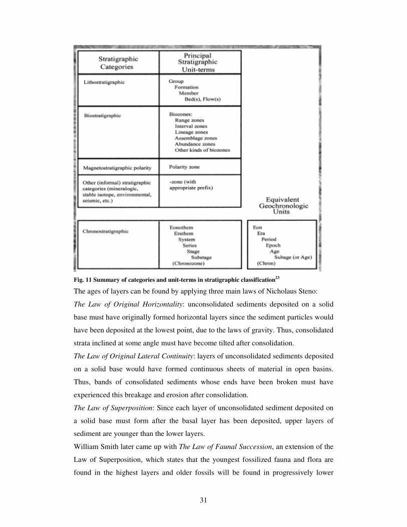
31

Fig. 11 Summary of categories and unit-terms in stratigraphic classification23

The ages of layers can be found by applying three main laws of Nicholaus Steno:

The Law of Original Horizontality: unconsolidated sediments deposited on a solid

base must have originally formed horizontal layers since the sediment particles would

have been deposited at the lowest point, due to the laws of gravity. Thus, consolidated

strata inclined at some angle must have become tilted after consolidation.

The Law of Original Lateral Continuity: layers of unconsolidated sediments deposited

on a solid base would have formed continuous sheets of material in open basins.

Thus, bands of consolidated sediments whose ends have been broken must have

experienced this breakage and erosion after consolidation.

The Law of Superposition: Since each layer of unconsolidated sediment deposited on

a solid base must form after the basal layer has been deposited, upper layers of

sediment are younger than the lower layers.

William Smith later came up with The Law of Faunal Succession, an extension of the

Law of Superposition, which states that the youngest fossilized fauna and flora are

found in the highest layers and older fossils will be found in progressively lower

32

layers.15

Stratigraphy gives information on post-depositional processes. These processes affect

soil deposition. It can completely be reversed or changed drastically by various

phenomena – hole digging or mud slides for example. To avoid misinterpretation,

long profiles or profiles form several units are required.

Cores, samples of these rock strata, must always be taken in order to effectively

analyse particular sequences of events as well as interpret how rock strata was

initially laid down.

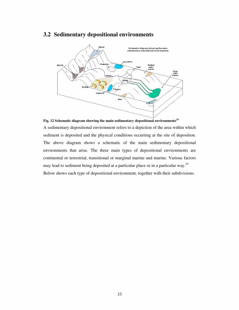
33

3.2 Sedimentary depositional environments

Fig. 12 Schematic diagram showing the main sedimentary depositional environments24

A sedimentary depositional environment refers to a depiction of the area within which

sediment is deposited and the physical conditions occurring at the site of deposition.

The above diagram shows a schematic of the main sedimentary depositional

environments that arise. The three main types of depositional environments are

continental or terrestrial, transitional or marginal marine and marine. Various factors

may lead to sediment being deposited at a particular place or in a particular way.25

Below shows each type of depositional environment, together with their subdivisions.

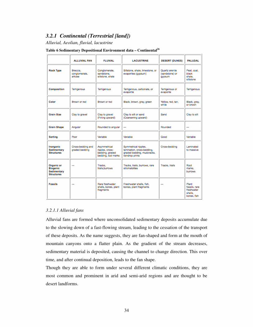
34

3.2.1 Continental (Terrestrial [land])

Alluvial, Aeolian, fluvial, lacustrine

Table 6 Sedimentary Depositional Environment data – Continental26

3.2.1.1 Alluvial fans

Alluvial fans are formed where unconsolidated sedimentary deposits accumulate due

to the slowing down of a fast-flowing stream, leading to the cessation of the transport

of these deposits. As the name suggests, they are fan-shaped and form at the mouth of

mountain canyons onto a flatter plain. As the gradient of the stream decreases,

sedimentary material is deposited, causing the channel to change direction. This over

time, and after continual deposition, leads to the fan shape.

Though they are able to form under several different climatic conditions, they are

most common and prominent in arid and semi-arid regions and are thought to be

desert landforms.

35

Several alluvial fans close to one another may converge to form a compound alluvial

fan, or bajada.27

Fig. 13 An alluvial fan in China’s XinJiang province28

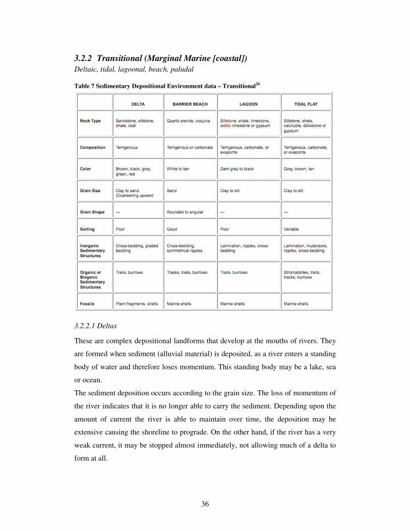
36

3.2.2 Transitional (Marginal Marine [coastal])

Deltaic, tidal, lagoonal, beach, paludal

Table 7 Sedimentary Depositional Environment data – Transitional

26

3.2.2.1 Deltas

These are complex depositional landforms that develop at the mouths of rivers. They

are formed when sediment (alluvial material) is deposited, as a river enters a standing

body of water and therefore loses momentum. This standing body may be a lake, sea

or ocean.

The sediment deposition occurs according to the grain size. The loss of momentum of

the river indicates that it is no longer able to carry the sediment. Depending upon the

amount of current the river is able to maintain over time, the deposition may be

extensive causing the shoreline to prograde. On the other hand, if the river has a very

weak current, it may be stopped almost immediately, not allowing much of a delta to

form at all.

37

In delta formation, the heaviest sediment is dropped first, for example, sand. Further

away from the mouth of the delta, finer sediment such as fine sand, silt and clay are

found. Because of this, distinct layers – topsets, foresets, bottomsets – are formed.29

Fig. 14 The shifting nature of the dynamic Mississippi River Delta over the last 4600 years

30

38

3.2.3 Marine (Marine [open ocean])

Shallow & deepwater marine: reef, shelf, floodplain

Table 8 Sedimentary Depositional Environment data – Marine26

3.2.3.1 Continental shelves

These refer to the gently sloping and extended perimeter of a continent that is

submerged under relatively shallow seas – shelf seas – as well as gulfs, and occupies

about 7% of the total ocean floor.

Sedimentary material from the continent flows down the continental slope and

accumulates at the base of the slope, resulting in the continental rise.

Continental shelves have gentle slopes and are relatively flat due to erosion and the

deposition of sediment during the periodic rise and fall over time of the sea covering

the shelf.

Continental shelves contain valuable resources, such as oil, gas and minerals. Organic

material accumulates on the continental shelf and over time is buried and transformed

by heat and pressure into oil and gas, which rises and is concentrated beneath

39

geologic traps. Oil and gas can be found on the continental shelf off the coasts of

California and Louisiana. Rocks on land, containing minerals, are carried to the ocean

by rivers. The minerals, after deposition in river channels and beaches on the exposed

continental shelf, are concentrated and sorted based on their density by waves and

river currents.31,32

Fig. 15 Diagram showing a continental shelf33

Other types also include evaporite and glacial depositional environments.

Sedimentary structures arise from these depositional environments. These physical

structures give an idea of the conditions that gave rise to them.

Bedding Planes are formed due to an interruption in bed formation – layers of

sediment. This is caused by erosion or a lack of deposition.

Channels are rivers that flow in elongated depressions.

Submerged bars and Dunes are formed from water and wind currents respectively.

The water currents carry sand or gravel along the bottom and the wind carries sand

along a beach or desert. Bar or dune migration occurs based on the direction in which

the water or wind is moving.

Ripples form from a water current or wave passing over sand or silt in shallow water.

These ripples can be considered to be mini bars or dunes.

Mudcracks are formed when water slowly evaporates from a muddy pool. This leaves

behind moist clay, which dries up and eventually cracks.

These structures give an idea about the conditions under which they were formed;

mudcracks, for example, tells that this is an area of alternating wet and dry periods.

When considering clastic and organic sediments, two processes may occur.

First, there may be deposition and accumulation of sediment in the depositional

environment. This is followed by burial of these by more sediment. Then, lithification

40

[cementation and compaction] of the accumulated sediment occurs leading to the

formation of sedimentary rock.

Also, there may be deposition, accumulation and burial of the sediment. However,

before lithification can occur, there is erosion and re-exposure of the buried sediment.

It, therefore, then goes through one or more new cycles of weathering: erosion –

transport – deposition – burial.25

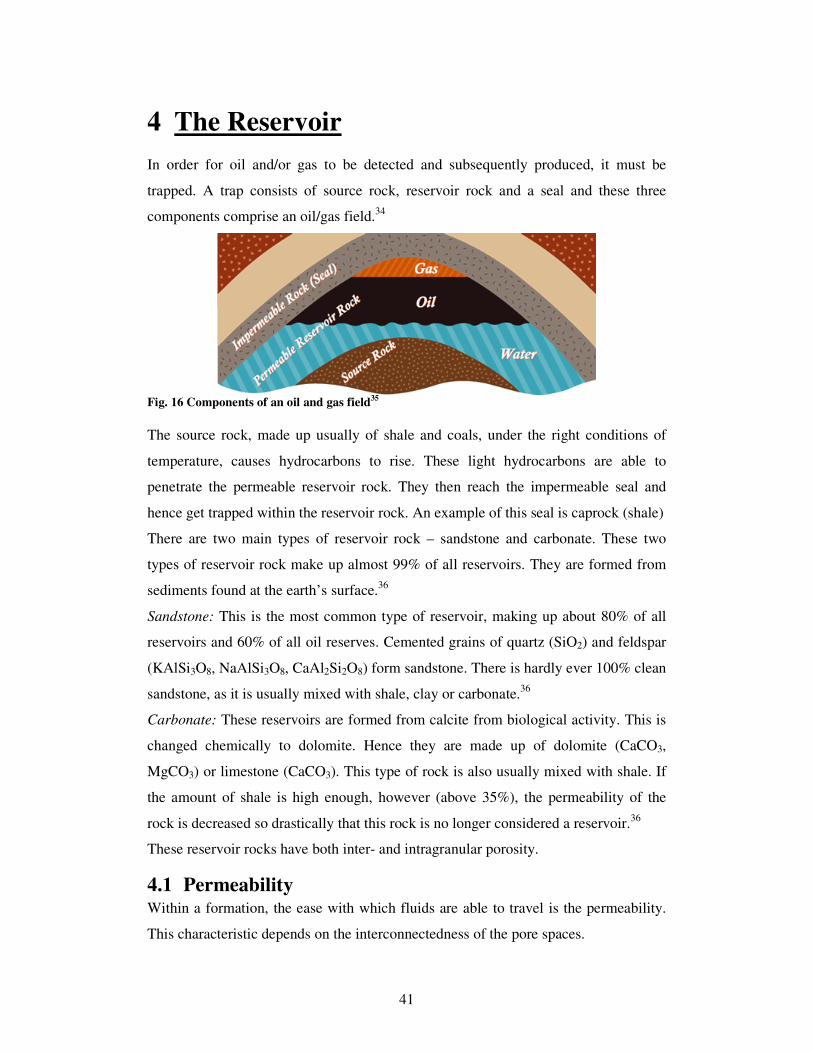
41

4 The Reservoir

In order for oil and/or gas to be detected and subsequently produced, it must be

trapped. A trap consists of source rock, reservoir rock and a seal and these three

components comprise an oil/gas field.34

Fig. 16 Components of an oil and gas field35

The source rock, made up usually of shale and coals, under the right conditions of

temperature, causes hydrocarbons to rise. These light hydrocarbons are able to

penetrate the permeable reservoir rock. They then reach the impermeable seal and

hence get trapped within the reservoir rock. An example of this seal is caprock (shale)

There are two main types of reservoir rock – sandstone and carbonate. These two

types of reservoir rock make up almost 99% of all reservoirs. They are formed from

sediments found at the earth’s surface.36

Sandstone: This is the most common type of reservoir, making up about 80% of all

reservoirs and 60% of all oil reserves. Cemented grains of quartz (SiO2) and feldspar

(KAlSi3O8, NaAlSi3O8, CaAl2Si2O8) form sandstone. There is hardly ever 100% clean

sandstone, as it is usually mixed with shale, clay or carbonate.36

Carbonate: These reservoirs are formed from calcite from biological activity. This is

changed chemically to dolomite. Hence they are made up of dolomite (CaCO3,

MgCO3) or limestone (CaCO3). This type of rock is also usually mixed with shale. If

the amount of shale is high enough, however (above 35%), the permeability of the

rock is decreased so drastically that this rock is no longer considered a reservoir.36

These reservoir rocks have both inter- and intragranular porosity.

4.1 Permeability Within a formation, the ease with which fluids are able to travel is the permeability.

This characteristic depends on the interconnectedness of the pore spaces.

42

The permeability that is parallel to a layer is usually higher than the permeability

perpendicular to the layer, with anisotropy ratios being very large. This holds for

reservoirs that had layers forming flat like blankets or pancakes. The anisotropy refers

to the difference in shape, make-up of physical characteristics of a formation. Its unit

is the mD (millidarcy) and its symbol is k. It can be calculated from Darcy’s formula:

Q = [kA(Pi – Po)]/µL

; where Q ≡ the (volumetric) flow rate measured in cm3/s or m

3/s

Po ≡ the outlet fluid pressure measured in Pa

Pi ≡ the inlet fluid pressure measured in Pa

µ ≡ the dynamic viscosity of the fluid measured in centipoise (cP)

L ≡ the length of the tube measured in cm or m

k ≡ the permeability of the sample measured in milliDarcy (mD)

A ≡ the area of the sample measured in cm2 or m

2

The conditions required for the Darcy formula to be able to be used include a laminar

flow, steady state, incompressible fluids and a homogeneous formation.5

The permeability is measured in the laboratory on core samples obtained from the reservoir.

The process is carried out by passing a fluid of known viscosity through the core sample of

known dimensions at a set rate, and measuring the pressure drop across the core. It can also

be carried out by setting the fluid to flow at a set pressure difference, and measuring the

flow rate produced.

The absolute permeability, k is derived when there is only one fluid found in the rock,

and the rock permeability is at its maximum.

Where there are two or more fluids found within the rock, their flow rates and

therefore individual permeabilities in the rock would differ. The individual

permeabilities depend on the saturation of the particular fluid in the rock. This is the

effective permeability, kw, ko, kg for water, oil and gas respectively. The value for all

effective permeabilities is always less than the absolute permeability of the rock.

The effective permeability can be written as a fraction of the absolute permeability of

the rock of any of the present fluids at 100% saturation. This is referred to as the

relative permeability, kr. Here, krw=kw/k, kro=ko/k, krg=kg/k for water, oil and gas

respectively.2

Grain size, grain sorting, fluid characteristics and porosity all affect the

permeability.5,37,38

43

4.2 Porosity This refers to the pore volume per unit volume of formation.

It is calculated as:

φ = Pore volume/Total bulk volume = (V – Vs)/V = Vp/V

; where Vs represents the volume occupied by the matrix.

The porosity within the main types of rock found in a reservoir differs greatly:

Dense carbonates – These are made up of limestones and dolomites. They usually

have very low porosity, if any.

Evaporites – These are salt, anhydrite, gypsum and sylvite. They also have very low

porosity.

For both dense carbonates and evaporites, the low porosity is due to the fact that the

pore space is very small, since the particles are well compacted.

Well-consolidated sandstones – These have porosity of between 10 and 15%.

Unconsolidated sandstones – Since these sandstones are unconsolidated, the pore

space is larger and therefore these have porosity of about 30% or more.

Shales/Clays – These have high porosity, usually of about 40%. This porosity is

usually water-filled however and due to the small size of the pores, they typically

have very low permeability.

Vugs and caves are known to be produced due to secondary porosity. This pore space

does not arise naturally in the rock but may occur due to the action of tectonic activity

or formation water movement on the rock matrix after deposition. It may also arise

due to the interaction between the drilling mud and shale.

Fractures, fissures and cracks may also increase porosity slightly. The larger the

porosity of the formation, the greater the amount of formation water found in the pore

space and consequently, the lower the resistivity.

The absolute porosity refers to the ratio of total pore space in the rock to that of the

bulk volume.

The effective porosity is the absolute or total porosity minus the clay volume.

There are several factors that affect the porosity. These include grain size, grain size

distribution, grain packing, grain shape, compaction and cementation.5

44

The sonic, neutron and density logs are the most common well-logging methods used

to determine the porosity of the rock being analysed, once the formation lithology is

known. The symbol for porosity is φ and it is measured as a percentage.

4.3 Water saturation The saturation of the formation is the fraction of the volume of pore fluid that is filled

with a specific fluid.

It is not possible to remove 100% of oil or water from a reservoir. There is always

some amount of each fluid that remains within the formation.

The irreducible water saturation, Swi, is the fraction of water in the pore space that

cannot be removed. It is known as the connate water and this arises due to capillary

forces that cause water to cling to the rock.

The residual oil saturation, Sor, is the fraction of oil in the pore space that cannot be

removed by ordinary fluid drives or recovery techniques.

There is a transition zone that occurs between the areas of 100% water saturation, Sw

and 100% oil saturation, So.

The longer the transition zone is, the lower the permeability and conversely a shorter

transition zone has a higher permeability.

The saturation of the residual hydrocarbons in the flushed zone can be calculated by:

Shr = (1 – Sxo)

; where Sxo is the saturation of the flushed zone

The saturation of hydrocarbons in the formations is calculated by:

Sh = (1 – Sw);

Sw being the saturation of the formation water

Therefore, the bulk volume of moveable oil = φ(Sxo – Sw)5

45

5 Well Correlation

5.1 Introduction

Once sandstone layers have been determined in various wells, it is important to find a

correlation between wells. The six wells analysed – 335R, 360R, 333R, 313R, 338R,

312R – were put together in a multi-well correlation to examine trends between them.

This also enabled a comparison between the layers found from the correlation and the

facies analysis, discussed in the next chapter.

Based on the multi-well correlation performed in IP, a general idea of the placement

of the wells was found. Seeing that no map was readily available, the wells were

given arbitrary coordinates in Petrel, and positioned accordingly, as seen in Fig. 18

Various modelling and imaging was then done in Petrel using the log information in

IP to generate models for the parameters being analysed.

5.2 Geological Description of the Komso Field

The Komso field is located in the Purovskoe region of the Yamalo-Nenets

Autonomous District in the Northern West Siberian Plain, on the left bank of

Pyakupur – a tributary of the river Pur – along the highway of Surgut-Urengov.

North-east of the field, at a distance of about 15 km, is the town of Gubkinsky, with a

population of 20,000 people. About 37 km away is the village of Purpe. On the

oilfield site, there are only settlements for rotating staff.

In 1966, gas deposits were found in the Cenomanian, and deposits of oil were found

further down in 1982. Test operation began in 1988, after appraisal drilling was

conducted in 1986.

Of the 195 wells of the Komso field, 9 of which are injection wells, 120 wells are

currently engaged in hydrocarbon production.

16 of the productive reservoirs in this field have production rates of exploration wells

to date ranging between 5-30%.

The climate of the area is continental, and is characterised by a negative average

annual air temperature of about -6.7°C, and a short 87-day frost-free period. There is

uneven precipitation, mainly during the warmer seasons, during periods of high

relative humidity and during winter.

46

The field is a part of the Nadym Pur oil and gas province, which, structurally and

tectonically, forms the central zone of the regional uplift. The geological section is

represented by the terrigenous-sedimentary Mesozoic-Cenozoic age, with a depth of

3600m, which are allocated complexes of Jurassic, Cretaceous, Paleogene and

Quaternary sediments.

There are 2 domes located within the Komso field – the East (15 - 20 km) and West

(10 - 15 km) domes. There are potential petroleum deposits associated with the Upper

Cretaceous (Cenomanian reservoir, containing free gas) and the Lower Cretaceous

(Valanginian-Albian oil-and gas-bearing reservoir) deposits.

The Komso field has quite a complex geological structure with a large number of oil

and gas reservoirs in a small margin. It contains 52 productive reservoirs, 10 of which

are gas-bearing, the others containing oil, gas and condensate. Geological oil reserves

of the Komso field are contained in 13 basic and 8 additional operating units.39

5.3 Description of the Core Sample

The sandstone found in this field is made up of small, dark-grey grains with feldspar,

quartz, mica and some amount of clay cement. Fissures and claystone nodules are

found along the contact line between the shaly and carbonised sandstones.

Fig. 17 Core sample – sandstone

40

47

Fig. 18 Mapping of the six wells using arbitrary coordinates for positioning in Petrel

5.4 Interactive Petrophysics

Six wells were analysed side by side in a multi-well correlation plot in the Senergy

Interactive Petrophysics (IP) program. This was to see where certain trends occurred

and where the similarities lay between them. Common sandstone layers within the

various wells were marked in IP in the correlation plot. The wells were added one at

a time, beginning with 2 wells. The addition of more wells changed and updated some

of the trends between them, taking into consideration each extra well that was added.

48

At some particular depth ranges, the matching of sandstone layers is better than at

other depth ranges. This helps to give an idea of where the wells are placed in relation

to one another in the actual field, as well as the general shape of the layer throughout

the six wells. There also seemed to be better correlation further towards the top and

towards the bottom of the wells. In the middle, there was a less clear correlation and

usually requires more careful analysis.

Below outlines the various sandstone layers found for each of the six wells and their

depth ranges.

Table 9 Top and base depths of each layer for each of the six wells

Well 335R 360R 333R 313R 338R 312R

Zone

Depth

(m)

Top

Base

Top

Base

Top

Base

Top

Base

Top

Base

Top

Base

Layer

A2 – – – – – – 1138.4 1162.2 1152.6 1167.4 – –

A3 – – – – – – 1171.0 1187.2 1167.5 1180.0 – –

A4 – – – – – – 1322.6 1347.6 1324.3 1347.0 – –

A5 1426.2 1455.6 1400.6 1427.0 1393.8 1424.0 1420.6 1442.2 1414.0 1433.7 1395.0 1408.4

A6 – – – – 1444.4 1463.0 1462.2 1486.0 1462.4 1486.2 – –

A7 – – – – 1532.2 1550.2 1559.0 1574.0 1537.0 1554.5 – –

A8 1601.6 1635.4 1598.0 1626.0 1583.4 1613.8 1613.6 1641.0 1609.3 1638.6 1603.4 1624.4

A9 1669.4 1690.6 1630.0 1660.4 1637.8 1659.8 1652.0 1674.6 1647.8 1673.7 1642.0 1660.0

B1 1720.0 1724.0 1693.8 1703.2 1689.0 1700.0 1691.0 1710.0 1685.1 1700.0 1672.4 1682.6

B2 1756.2 1781.6 1740.4 1766.8 1748.4 1774.0 1742.0 1792.2 1742.3 1782.4 1742.0 1752.0

B4 1882.0 1920.4 1872.0 1905.0 1863.6 1896.0 1855.0 1896.0 1854.0 1888.5 1835.0 1879.6

B5 1969.4 2021.2 1953.0 2012.0 1970.6 2017.4 1963.0 2021.0 1957.1 2036.4 1924.0 2007.4

B6 2069.6 2096.6 2039.8 2064.0 2032.0 2056.0 2036.2 2064.8 2037.1 2053.0 2019.4 2033.0

B7 2119.0 2124.8 2079.0 2093.0 2083.0 2093.4 2095.0 2120.0 2102.0 2124.1 2081.4 2094.8

B8 2207.8 2237.4 2184.0 2208.6 2158.8 2181.6 2164.6 2195.4 2184.8 2206.6 2173.4 2203.6

B9 2265.8 2305.8 2223.4 2277.0 2219.4 2271.0 2236.0 2290.6 – – 2229.2 2266.4

C1 2319.4 2331.2 2276.6 2304.6 2293.0 2306.0 2290.6 2305.0 2284.7 2293.1 2267.2 2289.0

C2 2342.8 2356.2 2306.0 2326.2 2325.4 2342.4 2321.4 2340.0 2320.2 2339.0 2305.0 2331.0

C4 2391.6 2443.4 2360.4 2405.0 2358.8 2397.0 2355.0 2409.0 2369.5 2416.5 2360.6 2410.0

C5 2459.0 2466.4 2427.0 2433.4 2424.0 2433.4 2431.0 2442.0 2431.0 2441.8 2414.2 2422.4

C6 2476.6 2525.8 2443.6 2487.8 2433.6 2489.6 2454.6 2489.0 2451.0 2486.4 2427.4 2447.4

C7 2530.2 2556.2 2487.8 2512.4 2494.0 2520.0 2504.0 2537.6 2508.7 2537.8 2468.6 2499.4

C8 2582.8 2596.6 2538.0 2554.4 2541.4 2555.4 2542.0 2560.6 2548.0 2559.5 2514.0 2539.0

C9 2614.6 2646.0 2571.8 2610.0 2577.4 2608.6 2577.0 2598.0 – – 2581.4 2606.2

5.5 Petrel

5.5.1 Mapping

The six chosen wells were first shown in a map window [Window–New Map

window] in Petrel. A New Well Folder [Insert–New Well Folder] was inserted and

the six wells inserted into this folder [Insert–New Well]. According to the scale of the

map in the map window, arbitrary x- and y-coordinates were given accordingly for

each well, so they each had their own position in the map. These coordinates were

49

based on the positioning of the wells in IP. It is important to also add the Bottom MD

value at this point to denote the length of the well’s pipe.

5.5.2 IP Log Data

The log data for each well from IP was then imported into Petrel [Right-click on

well–Import (on Selection)–Select relevant file with File type: Well logs (ASCII)

(*.*)]. The various wells can now be seen in a 3D window [Window–New 3D

window]. The log information can now be displayed in a Well Section window

[Window–New Well Section window]

Fig. 19 Initial log plot data for Well 312R showing depth, SP and resistivity curves

5.5.3 Sections

In the models pane, a skeleton of the top, mid and base reservoirs is inserted by

choosing the Make Simple Grid process [Processes Pane–Utilities Folder–Make

Simple Grid]. In the Input tab, the top and base limits were chosen to coincide with

the length of the pipe created. A Z-value (Bottom MD) of -3000 was chosen for the

length of the pipe so the top and base limits chosen were -500 and -2500 respectively.

In the Geometry tab, Xmin,max and Ymin,max values were chosen according to the

positioning of the wells in the map window. The minimum values are chosen to be

50

slightly lower than the lowest x- and y-values for each well and the maximum values

chosen to be slightly higher.

5.5.4 Horizons

The top and base horizons for each layer were made in the well section window by

creating a Well tops folder in the Input pane [Insert–New well tops]. By expanding

the Well tops folder, horizons were created within the Stratigraphy folder, by clicking

on the Add new well top surface in the function bar. A top and base was made for

each layer (from A2 to C9) and these were connected throughout all six wells. In

order to change the depth of a particular layer in a particular well, ensuring the

Create/edit well tops button was selected in the function bar, the top or base layer in

the well section window was right-clicked, and the depth changed.

5.5.5 Models

Surfaces

Horizons were again made for each layer – top and base – this time in the Models

pane [Processes pane–Structural Modelling–Make horizons]. The top and base

horizons previously created in the Input Pane [Input pane – Well tops – Stratigraphy]

were then placed into the Make horizons dialog box that opens, by clicking the

Append item in the table button to insert a row. The layers were entered one by one,

inserting the top and base for one layer, before moving on to the next.

Once all these horizons have been created, the horizons folder in the Models pane can

be expanded and the horizons selected. In the Models pane, the Edges button can be

selected in order to view the connection between a top and base layer. The Zone filter

button can be expanded and different zones turned on or off in order to see either all

the horizons, as well as their top and base connections, or perhaps the top and base

connection for one particular layer only.

51

(a) (b)

Fig. 20 Model of various sandstone layers without(a) and with(b) shale layers across the six wells

Below shows the multi-well correlation of each of the sandstone units through the six

wells generated in Petrel.

52

Fig. 21 Multi-well correlation generated in Petrel showing various sandstone layers

53

6 Facies Analysis & Modelling

The term facies refers to the depositional setting of the rock.1 It encompasses all of

the characteristics of a particular rock unit. For example, there may be a "tan, cross-

bedded oolitic limestone facies". The characteristics of the rock unit come from the

depositional environment. Every depositional environment puts its own distinctive

imprint on the sediment, making a particular facies. Thus, a facies is a distinct kind of

rock for that area or environment.41

Facies refers to a body of rock that has specific, distinctive characteristics and forms

under certain conditions of sedimentation, reflecting a particular process, set of

conditions, or environment. It should differ from those bodies of rock above, below

and laterally adjacent to it. Facies can be grouped into facies associations or

subdivided into subfacies. The idea of facies has been used for centuries in order to

analyse and determine areas of oil, coal and mineral ores.21

6.1 Types Facies are distinguished based on the various types of characteristics the sedimentary

rock possesses. Once a core of the rock is taken, or an outcrop is analysed, facies can

be defined based on the dominant aspect of the rock.

Biofacies – this is the term to refer to the sedimentary rock that has its biological

content as the dominant aspect

Ichnofacies – this is the facies that is defined based on the presence of trace fossils

Lithofacies – if the physical and chemical characteristics of the sedimentary rock are

its dominant attribute

Microfacies – this term is used, especially with carbonates, where the major attributes

are seen in a very small section of the rock

A = Sandstone facies (beach environment)

B = Shale facies (offshore marine environment)

C = Limestone facies (far from sources of terrigenous input)

Each depositional environment grades laterally into other environments. This is

known as facies change when analyzing rock record.41

54

6.2 Modelling Facies analysis refers to the interpretation of rocks and sediments for the purpose of

reconstructing the processes that were responsible for the original deposition.

Facies models can be created based on various classifications. They may be formed

based on direct descriptive classifications, from actual observable and measurable

features. They may be formed in an attempt to determine the original processes that

led the rock to be formed and deposited in the way that it was initially. They may also

be based on an attempt to regenerate the environment in which the rock was formed

and deposited.

Several facies models have also been formed to take into account external features

such as changes in tectonics, climate, type of sediment and sea level.

Advances in technology over time have allowed more sophisticated and intricate

facies models to be developed.21

There are several types of facies models:

Lithofacies model (Descriptive classifications): These are divided into classes, groups

and individual facies. Each classification is based upon different attributes. The

classes are distinguished based on grain size, internal organisation and composition,

the groups are based on internal structure and texture organisation and the individual

facies are based on internal structure, bed thickness, texture and composition.

Common lithofacies models were created for deep-water facies and alluvial facies.

Process facies model: This model is based on the generation of information about

how the sediment was originally formed and deposited – the formative processes that

led to how rock strata are positioned today. The names of these models have an –ite

ending, an example being the turbidite model, which helped in distinguishing between

descriptive and genetic characteristics of facies. It is based on the generation of a

turbidity current which explained the co-existence of shallow water containing

shallow water fossils and shales containing deep water pelagic fossils. Debrites are

massive sandstones formed as sandy debris flows. Other examples include tidalites,

which are the facies that arise from tidal currents due to the twice-daily rise and fall of

tides. They have a distinctive pattern of cross beds. Contourites are the facies that

arise from contour currents that parallel contours on the continental slope and rise.

These can range from fine terrigenous sand, to silt, to clay, to biogenic sediment.

55

Contourites made up primarily of biogenic sediment are extremely similar to

pelagites.

Environmental facies model: The type of environment in which facies were formed is

just as important as the way in which they were formed. Similar formative processes

may occur in completely different types of environments. It is therefore easier for

facies analysis, if facies are grouped into facies associations as opposed to being

analysed separately. These facies associations are based on some genetic or

environmental similarities.

Allocyclic sequence stratigraphic model: It is always possible that facies models may

arise due to external factors and forces. Tectonic activity has been highlighted as one

of the most common of these external forces.

6.3 Transgression & Regression Transgression means that water depths are increasing. In a transgressive sequence the

energy and sediment grain size will decrease higher up in the stratigraphic column -

also known as fining or deepening upward.

Regression of ocean waters indicates that water depths will get shallower so grain size

will increase and energy will increase - known as coarsening or shallowing upward.

Transgression - sea level rise

Regression - sea level drop

Fluctuations in sea level are caused by conditions such as:

1. Changes in the size of the polar ice caps, due to climatic changes

- Melting of ice caps leads to sea level rise (transgression) - it has been calculated that

the complete melting of the Antarctic Ice Sheet would cause a sea level rise of 60 - 70

meters.

- Growth of ice caps leads to a drop in sea level (regression) - calculations show that

sea level was as much as 100 meters lower than at present at the height of the last Ice

Age glaciation. Much of the Continental Shelf area would have been exposed and dry.

56

2. Rate of sea floor spreading - during times of rapid sea floor spreading and

submarine volcanism, the ocean ridge system is enlarged by the addition of lava,

displacing water onto the edges of the continents (transgression).

3. Localized subsidence or uplift of the land - In the 8000–10,000 years since the

melting of the last glacial ice sheet over North America, parts of Canada have risen

due to isostatic uplift by up to 300 meters.41

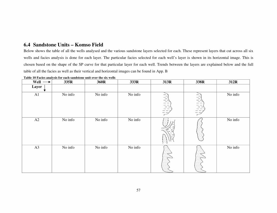
57

6.4 Sandstone Units – Komso Field Below shows the table of all the wells analysed and the various sandstone layers selected for each. These represent layers that cut across all six

wells and facies analysis is done for each layer. The particular facies selected for each well’s layer is shown in its horizontal image. This is

chosen based on the shape of the SP curve for that particular layer for each well. Trends between the layers are explained below and the full

table of all the facies as well as their vertical and horizontal images can be found in App. B

Table 10 Facies analysis for each sandstone unit over the six wells

Well 335R 360R 333R 313R 338R 312R

Layer

A1

No info No info No info

No info

A2


No info

A3


No info

58

A5

A8

A9

B1

59

B2

B4

B5

B6

60

B7

B8

B9

disappear

C1

61

C2

а)

б)

в)

а)

б)

в)

а)

б)

в)

C4

C5

C6

62

C7

C8

C9

No info

63

6.4.1 Description

This analysis takes place from the greatest depth to the shallowest, ie from layer C9,

moving upwards to layer A1.

C9: This has very clear regressive bars. As mentioned before, there is coarsening

upwards, giving the triangular shape of the SP log as shown in number 16 of App. B.

The well information for Well 338R is missing, however the same facies shape can be

seen for the remaining wells.

C8: As it is known that the sea water is always flowing, it is possible for there to be

changes in the movement of the sea. Here, the first three wells form transgressive

bars, whilst the last three retain the regressive bars from the lower layer.

C7: Bars form along the shoreline. If these bars are strong and stable, it is possible for

lagoons to form between the shore and the bar. However, if this bar is not particularly

stable, as seems to be the case in this layer, it is possible for the water currents from

the river to break through, forming the head parts of breaking currents. The last two

wells have the washouts of breaking currents as the river breaks through the bar and

begins to spread. The first three wells still remain transgressive bars as before.

C6: Since there has been transgression of the sea, water comes further onto the shore,

which may lead to waterflooding and cause some bars to be underwater. This is what

gives rise to the underwater slope of the delta. As rivers flow and come into contact

with the sea, their momentum is lost and they begin to deposit sediment. The various

river channels spread out as ‘sleeves’ and this is the case for the first three wells, as

well as well 338R. From layer C7 to this layer, it is possible that the angle of flow of

the river has changed, to the west, seeing that the head part of breaking current in well

313R becomes the washouts of breaking currents in well 312R. When water from the

river and water from the sea collides and interacts, it is possible for a change in

direction of the water to occur.

C5: Once again, as with flow and movement of the sea water, there is regression,

forming these regressive bars. The sleeves of the deltas carry a lot of sand. This is

eventually deposited and accumulated, also leading to the formation of regressive

bars.

C4: Underwater slope of deltas are formed in most of these wells. In wells 313R and

338R, it can be seen that transgressive bars are formed.

64

C2: If these stable bars do not exist, instead of lagoons, it is possible for shelves to

form, as is the case with wells 335R, 360R and 313R. The sleeves of the delta do not

only carry sand, but may also carry shale. Here, sedimentary rock of shallow shelves

is found.

C1: Mouth bars are formed at wells 333R and 313R. It is possible for beach ridges to

form on the sides of these mouth bars since as water flows to and fro it may push sand

up in a certain area, forming these ridges. The beach ridges are formed at wells 360R

and 312R as it can be seen there is a change from transgressive to regressive bars at

wells 335R and 338R.

B9: Shallow river beds of shallow rivers appear for all wells except 338R. There may

be more sandy conditions here, with a possible extension of the shoreline. There is a

loss of the sandstone layer for well 338R. This layer can be considered an

intermediate layer, or a region of stability. This explains why it is mainly shallow

beds that occur here, since there is not any major movement of water here.

B8: Transgressive bars are formed for wells 335R, 360R, 313R and 338R. This is

therefore where the sea water is flowing onto the shore. Where the shallow beds are

maintained, for wells 333R and 312R, this can be considered to be washouts of these

transgressive bars.

B7: The first three wells (335R, 360R, 333R) are very thin layers, which form

transgressive bars. This layer gets thicker in wells 313R and 338R and becomes more

of a shallow river bed in well 338R. The layer becomes slightly thinner again in well

312R and again forms the transgressive bar. From the previous layer to this one, there

is a continued change in the direction of the river water. There is again movement to

the west.

B6: Again there is movement of sea water, transgression, forming the underwater

slope of the delta in well 335R. Transgression of the river is seen in the remaining

wells.

B5: The underwater slope of the delta is formed in these wells. It seems that for well

313R, it is possible that a valley of a deltaic complex is formed.

B4: Again, there is further transgression of the river.

B2: Continuous transgression of the river.

B1: Now, there is regression as the movement of the river changes.

A9: Again, a change to transgression. Usually the periods of regression and

transgression are long. It is, however, possible that there are temporary periods of

65

regression and transgression. For regression, for example, this may arise if there are

sudden periods of hot weather where there will be loss of water close to the shore (as

opposed to the ocean pulling back the water)

A8: Shallow beds are formed as further transgression occurs.

A5: Transgressive bars are continued to be formed.

A3: There is only information for wells 313R and 338R for this layer. Transgression

bars are formed here from transgression of the river further onto the shore.

A2: Again only wells 313R and 338R have log information. As there is no

information for the other wells, it is possible to assume that there is the head part of

breaking currents forming in another well forming the washouts of these breaking

currents for well 313R. Regressive bars form for well 338R.

A1: Here also, there is only information for wells 313R and 338R for this layer. This

is a very shaly layer and represents open sea and large sea gulfs.

It can be seen that there is a cycle of regression of the sea water between layers C9 –

C5, where regressive bars are formed. This is followed by a cycle of transgression

from layer C4 to C2, with transgressive bars. Regressive bars are again formed in

layer C1. Layer B9 has a period of stability, or can be considered an intermediate

stage and then another cycle of transgression occurs, between layers B9 and B2. In

this cycle, there are some periods of waterflooding, but the major occurrence here is

transgression and the formation of transgressive bars. B1 has regression of the

seawater and regressive bar formation and from A9 to A1 has regular flow of the sea

water, onto the shore and back into the sea with transgression being the dominant

process. These trends are also evident in Fig. 23, described further below.

66

Top

(a) Base

Top (b) Base

Top (c) Base

67

Top (d) Base

Top (e) Base

Fig. 22 Top and base contour lines for layers B5 (a), C1 (b), C4 (c), C6 (d) & C7 (e)

The contour lines here show the top and base description for select layers. These are

layers where significant changes in the movement of the sea occurred, leading to the

formation of distinct facies.

For example, with layer C7, the head parts of breaking currents are formed here,

where unstable bars are present, and then the washouts of breaking currents. This is

depicted in the top and base contour layers as there is a change in the region,

seemingly a breakthrough, surrounding the first four wells.

68

6.5 Clay Volume

The SP log in IP was used to determine the clay volume. Even though it gives small deflections for thin layers, it is insensitive to other

surrounding factors. Clay volume is important to calculate seeing that it takes up some of the pore space within rocks.

Table 11 Minimum, maximum and reference depth SP values for clay volume calculation

335 360 333 313 338 312

SP SP SP SP SP SP

Min Max Log Ref.

depth

Min Max Log Ref.

depth

Min Max Log Ref.

depth

Min Max Log Ref.

depth

Min Max Log Ref.

depth

Min Max Log Ref.

depth

A2 – – – – – – – – – – – – 17 61 19 1150.6 27 71 29 1156.8 – – – –

A3 – – – – – – – – – – – – 26 66 27 1183.0 26 71 29 1178.6 – – – –

A4 – – – – – – – – – – – – 27 68 33 1333.0 19 71 24 1345.0 – – – –

A5 44 89 49 1429.0 19 79 25 1414.4 12 65 26 1404.4 14 67 18 1429.4 16 75 19 1422.2 41 65 47 1407.2

A6 – – – – – – – – 10 62 19 1456.4 17 68 18 1478.0 19 74 34 1478.6 – – – –

A7 – – – – – – – – 5 63 13 1542.0 17 68 22 1569.0 16 76 21 1546.2 – – – –

A8 29 87 30 1625.4 6 81 15 1614.8 5 66 13 1606.0 15 67 20 1630.2 14 76 21 1617.9 52 67 56 1622.6

A9 44 89 63 1672.8 12 79 28 1641.0 5 65 11 1641.8 18 66 19 1669.0 23 76 25 1654.6 43 69 51 1657.0

B1 46 84 55 1722.8 14 83 31 1695.4 2 64 7 1693.0 16 67 21 1695.4 13 75 17 1692.0 35 70 49 1679.0

B2 25 89 33 1763.2 14 79 21 1765.2 2 64 19 1764.4 5 65 12 1756.2 6 79 15 1764.0 16 67 35 1745.2

B4 8 91 19 1910.0 24 87 28 1901.0 -2 68 13 1882.0 6 68 13 1879.0 4 79 11 1882.2 20 75 45 1857.0

B5 7 90 10 1984.4 -5 88 2 1982.6 -10 68 2 1996.2 2 71 9 2000.4 -6 81 -1 1976.3 13 78 21 1958.8

B6 7 89 9 2080.8 1 87 5 2047.0 -5 72 15 2043.8 -2 69 10 2049.0 4 84 7 2046.9 17 76 33 2025.4

B7 19 93 26 2123.0 -3 85 9 2089.2 14 71 20 2085.8 1 69 8 2114.6 -3 86 3 2113.8 17 76 27 2092.6

B8 2 91 11 2215.0 -3 87 14 2193.2 -15 74 -1 2176.4 -2 68 2 2188.2 -12 83 -7 2199.0 0 74 2 2184.8

B9 2 90 6 2271.4 -16 85 -10 2238.6 -13 74 -7 2228.0 -11 63 -7 2253.4 – – – – 10 83 17 2233.6

C1 20 94 34 2319.8 -3 85 5 2287.0 -7 75 4 2296.0 -3 67 4 2295.0 -1 85 5 2291.5 19 84 14 2263.0

C2 1 93 5 2346.2 2 88 11 2312.8 -4 75 6 2328.2 -7 69 1 2333.4 -14 86 -9 2334.5 17 86 27 2314.0

C4 1 95 10 2402.0 -10 84 -1 2371.2 -12 76 1 2366.4 -5 69 1 2387.0 -14 86 -7 2400.0 9 87 16 2403.2

C5 22 93 30 2462.8 -2 59 2 2428.8 7 76 15 2429.8 2 71 17 2435.4 -11 89 2 2440.0 35 85 44 2417.6

C6 -9 80 3 2485.4 -12 84 3 2464.6 -8 76 1 2441.6 -12 56 -4 2474.6 -16 83 -1 2466.7 12 83 20 2439.8

C7 -6 84 8 2546.6 -5 82 1 2505.0 -3 76 2 2514.4 -6 71 14 2523.0 -15 88 3 2519.9 25 95 31 2491.4

C8 -7 94 24 2592.0 -8 87 2 2540.4 1 75 4 2551.4 3 72 4 2556.4 -18 57 -1 2556.8 25 94 40 2524.4

C9 -10 92 10 2622.4 -11 94 2 2580.2 -9 74 -1 2585.2 -3 70 4 2588.6 – – – – 34 94 46 2598.0

Clay volume = [SPclean – SPlog] / [SPclean – SPshale] or [Min – log] / [Min – Max]

; where

Min = SPclean (clean sandstone)

Max = SPshale

log = Splog

69

Table 12 Clay and sand volumes for each layer of each well Layer 335 360 333 313 338 312 Mean Vsh Mean Vsand

(1 – Mean

Vsh)

A2 – – – 0.045 0.045 – 0.045 0.955

A3 – – – 0.025 0.067 – 0.046 0.954

A4 – – – 0.146 0.096 – 0.121 0.879

A5 0.111 0.100 0.264 0.075 0.051 0.250 0.142 0.858

A6 – – 0.173 0.020 0.273 – 0.155 0.845

A7 – – 0.138 0.098 0.083 – 0.106 0.894

A8 0.017 0.120 0.131 0.096 0.113 0.267 0.124 0.876

A9 0.422 0.239 0.100 0.021 0.038 0.308 0.188 0.812

B1 0.237 0.246 0.081 0.098 0.065 0.400 0.188 0.812

B2 0.125 0.108 0.274 0.117 0.123 0.373 0.187 0.813

B4 0.133 0.063 0.214 0.113 0.093 0.455 0.179 0.822

B5 0.036 0.075 0.154 0.101 0.057 0.123 0.091 0.909

B6 0.024 0.047 0.260 0.169 0.038 0.271 0.135 0.865

B7 0.095 0.136 0.105 0.103 0.067 0.169 0.113 0.888

B8 0.101 0.189 0.157 0.057 0.053 0.027 0.097 0.903

B9 0.045 0.059 0.069 0.054 – 0.096 0.065 0.935

C1 0.189 0.091 0.134 0.100 0.070 0.071 0.085 0.916

C2 0.043 0.105 0.127 0.105 0.050 0.145 0.096 0.904

C4 0.096 0.096 0.148 0.081 0.070 0.090 0.097 0.903

C5 0.113 0.000 0.116 0.217 0.130 0.180 0.137 0.863

C6 0.135 0.156 0.107 0.118 0.152 0.113 0.130 0.870

C7 0.156 0.069 0.063 0.260 0.175 0.086 0.135 0.865

C8 0.307 0.105 0.041 0.014 0.227 0.217 0.152 0.848

C9 0.196 0.124 0.096 0.096 – 0.200 0.142 0.858

Clay volume can also be read from the IP program. The plot is generated from

Interpretation – Clay Volume in IP and the clay volume values found at the same

reference depth chosen for the log value of the SP for each layer of each well. There

may be slight differences between the manual and IP clay volume values. This is

because in general the manual calculation is an over estimation (assumes there is less

clay volume than there really is) since it is based on the SSP, which is an estimated

value. In addition to this, the calculation of clay volume from the equation uses one

reference point depth whilst the calculation from IP uses the entire SP curve,

consisting of several points, to obtain the clay volume. In this report, the manual

calculation is used. Though not shown here, the values of clay volume from IP

corroborated those obtained from the manual calculation.

70

6.5.1 Sand, Shale distribution of Facies Models

A2 resulting facies fractions:

------------------------------------------------

Sand: 93.96 %

Shale: 6.04 %

------------------------------------------------


------------------------------------------------

Sand: 95.19 %

Shale: 4.81 %

------------------------------------------------


------------------------------------------------

Sand: 89.89 %

Shale: 10.11 %

------------------------------------------------


------------------------------------------------

Sand: 82.58 %

Shale: 17.42 %

------------------------------------------------


------------------------------------------------

Sand: 82.43 %

Shale: 17.57 %

------------------------------------------------


------------------------------------------------

Sand: 83.92 %

Shale: 16.08 %

------------------------------------------------


------------------------------------------------

Sand: 76.98 %

Shale: 23.02 %

------------------------------------------------


------------------------------------------------

Sand: 77.41 %

Shale: 22.59 %

------------------------------------------------

B1 resulting facies fractions:

------------------------------------------------

Sand: 85.02 %

Shale: 14.98 %

------------------------------------------------


------------------------------------------------

Sand: 79.01 %

Shale: 20.99 %

------------------------------------------------


------------------------------------------------

Sand: 84.92 %

Shale: 15.08 %

------------------------------------------------


71

------------------------------------------------

Sand: 89.71 %

Shale: 10.29 %

------------------------------------------------


------------------------------------------------

Sand: 94.13 %

Shale: 5.87 %

------------------------------------------------


------------------------------------------------

Sand: 84.76 %

Shale: 15.24 %

------------------------------------------------


------------------------------------------------

Sand: 91.77 %

Shale: 8.23 %

------------------------------------------------


------------------------------------------------

Sand: 97.35 %

Shale: 2.65 %

------------------------------------------------

C1 resulting facies fractions:

------------------------------------------------

Sand: 93.16 %

Shale: 6.84 %

------------------------------------------------


------------------------------------------------

Sand: 85.65 %

Shale: 14.35 %

------------------------------------------------


------------------------------------------------

Sand: 95.05 %

Shale: 4.95 %

------------------------------------------------


------------------------------------------------

Sand: 93.76 %

Shale: 6.24 %

------------------------------------------------


------------------------------------------------

Sand: 86.36 %

Shale: 13.64 %

------------------------------------------------


------------------------------------------------

Sand: 79.71 %

Shale: 20.29 %

------------------------------------------------


------------------------------------------------

Sand: 88.21 %

Shale: 11.79 %

------------------------------------------------


------------------------------------------------

Sand: 84.29 %

Shale: 15.71 %

------------------------------------------------

72

Above shows the sand-to-shale ratios for each layer, used to determine the facies

models.

Fig. 23 Facies model of all sandstone units across the six wells

The figure above depicts each of the layers and their sand-shale distributions.

It shows the separation of sandstone bodies by shale. Shale located at depth of 2200m

is moving west until about 2000m. In the next layer there seems to be some

interruption where it disappears and reappears at about 1900m. There is again a

repetition of this westward movement of shale up to about 1500m. These depictions,

in general, match the trend of the facies analysis in Table 10.

Five representative layers are shown below to see how these facies models were

determined separately.

73

Fig. 24 Facies model representation of three layers (layers A5, B5 & C5)

74

7 Calculation of Petrophysical Parameters

7.1 Formation Water Resistivity & Salinity These parameters were found using various Schlumberger charts as well as the SP

log. Well 312R, in Table 13, will be used as an example in this chapter, with the

information on the remaining five wells found in App. C

Rxo and Rt were found from the GZ2 and GZ4 resistivity plots in IP respectively.

After finding Essp from the SP log in IP, Schlumberger chart SP-1 is used to find

Rmfeq and Rweq [see Fig. 25]

Fig. 25 Rweq and Rmfeq determination from Essp

42

Rw is then found from Rweq using Schlumberger chart SP-3 below.

75

Fig. 26 Rweq vs Rw and formation temperature

42

Using this value of Rw and Schlumberger Chart Gen-6, the salinity can be determined.

Fig. 27 Salinity determination from Rw and formation temperature

42

76

Table 13 Resistivity and salinity information for Well 312R

Layer ∆∆∆∆Usp

(mV)

Ref.

depth Rt (ΩΩΩΩ-m) Rm (ΩΩΩΩ-m) Rmf (ΩΩΩΩ-m) Vsp Essp =

∆∆∆∆Usp/Vsp

(mV)

Rmfeq/Rweq Rmfeq (ΩΩΩΩ-m) Rweq (ΩΩΩΩ-m) Rw (ΩΩΩΩ-m) Salinity

(g/L)

A2 – – – – – – – – – – – –

A3 – – – – – – – – – – – –

A4 – – – – – – – – – – – –

A5 -24 1407.2 4.78 3.0 2.4 1 -24 2.0 0.08 0.040 0.0475 65.0

A6 – – – – – – – – – – – –

A7 – – – – – – – – – – – –

A8 -15 1622.6 6.11 3.0 2.4 1 -15 1.6 0.06 0.034 0.0425 80.0

A9 -26 1657.0 6.64 3.0 2.4 1 -26 2.0 0.08 0.040 0.0475 65.0

B1 -35 1679.0 6.07 3.0 2.4 1 -35 2.6 0.15 0.058 0.0700 45.0

B2 -51 1745.2 13.3 3.0 2.4 1 -51 4.0 0.35 0.088 0.1000 30.0

B4 -55 1857.0 10.3 3.0 2.4 1 -55 4.6 0.50 0.109 0.1200 25.0

B5 -65 1958.8 3.47 3.0 2.4 1 -65 6.0 0.80 0.133 0.1400 20.0

B6 -59 2025.4 9.57 3.0 2.4 1 -59 5.2 0.60 0.115 0.1300 22.0

B7 -59 2092.6 10.1 3.0 2.4 1 -59 5.2 0.60 0.115 0.1300 22.0

B8 -74 2184.8 7.53 3.0 2.4 1 -74 8.0 1.36 0.170 0.2000 14.0

B9 -73 2233.6 4.43 3.0 2.4 1 -73 8.0 1.36 0.170 0.2000 14.0

C1 -65 2263.0 2.98 3.0 2.4 1 -65 6.0 0.80 0.133 0.1400 20.0

C2 -69 2314.0 3.76 3.0 2.4 1 -69 7.0 1.00 0.143 0.1500 18.5

C4 -78 2403.2 3.35 3.0 2.4 1 -78 9.0 1.62 0.180 0.2100 13.0

C5 -50 2417.6 4.3 3.0 2.4 1 -50 4.0 0.35 0.088 0.1000 30.0

C6 -71 2439.8 4.0 3.0 2.4 1 -71 7.0 1.00 0.143 0.1500 18.5

C7 -70 2491.4 9.02 3.0 2.4 1 -70 7.0 1.00 0.143 0.1500 18.5

C8 -69 2524.4 5.42 3.0 2.4 1 -69 7.0 1.00 0.143 0.1500 18.5

C9 -60 2598.0 11.0 3.0 2.4 1 -60 5.2 0.60 0.115 0.1300 22.0

77

7.2 Permeability

Permeability was found using porosity values, with the equation:

k1/2

= (250 * φφφφ3) / Swi

; where Swi is the irreducible water saturation, here assumed to be the minimum value

of 0.1

Table 14 Permeability information for Well 312R

312 Layer φφφφ k

A2 – –

A3 – –

A4 – –

A5 0.399 12.602

A6 – –

A7 – –

A8 0.451 15.144

A9 0.420 13.610

B1 0.311 8.672

B2 0.161 3.230

B4 0.123 2.157

B5 0.132 2.398

B6 0.239 5.842

B7 0.191 4.174

B8 0.208 4.743

B9 0.206 4.675

C1 0.203 4.573

C2 0.136 2.508

C4 0.147 2.818

C5 0.350 10.353

C6 0.170 3.505

C7 0.234 5.660

C8 0.234 5.660

C9 0.191 4.174

7.3 Porosity & Water Saturation The Archie formulae were used to find porosity and water saturation, shown below.

Porosity, φ = [(a*Rmf)/Rxo]1/m

Water Saturation, Sw = [(a/φm

)*(Rw/Rt)]1/m

; where a=0.64 and m=1.74, which are the standard Schlumberger values used for

porosity calculation.

78

Table 15 Porosity and water saturation information for Well 312R

Layer Ref.

depth Rmf (ΩΩΩΩ-m) Rxo (ΩΩΩΩ-m) Rt (ΩΩΩΩ-m) Rw (ΩΩΩΩ-m) a m φφφφ Sw Shc = 1-Sw

A2 – – – – – – – – – –

A3 – – – – – – – – – –

A4 – – – – – – – – – –

A5 1407.2 2.4 7.6 4.78 0.0475 0.64 1.74 0.399 0.137 0.863

A6 – – – – – – – – – –

A7 – – – – – – – – – –

A8 1622.6 2.4 6.15 6.11 0.0425 0.64 1.74 0.451 0.099 0.901

A9 1657.0 2.4 6.96 6.64 0.0475 0.64 1.74 0.420 0.108 0.892

B1 1679.0 2.4 11.7 6.07 0.0700 0.64 1.74 0.311 0.191 0.809

B2 1745.2 2.4 36.7 13.3 0.1000 0.64 1.74 0.161 0.288 0.712

B4 1857.0 2.4 58.6 10.3 0.1200 0.64 1.74 0.123 0.486 0.514

B5 1958.8 2.4 51.8 3.47 0.1400 0.64 1.74 0.132 0.924 0.076

B6 2025.4 2.4 18.5 9.57 0.1300 0.64 1.74 0.239 0.273 0.727

B7 2092.6 2.4 27.4 10.1 0.1300 0.64 1.74 0.191 0.332 0.668

B8 2184.8 2.4 23.7 7.53 0.2000 0.64 1.74 0.208 0.463 0.537

B9 2233.6 2.4 24.1 4.43 0.2000 0.64 1.74 0.206 0.635 0.365

C1 2263.0 2.4 24.7 2.98 0.1400 0.64 1.74 0.203 0.659 0.341

C2 2314.0 2.4 49.6 3.76 0.1500 0.64 1.74 0.136 0.895 0.105

C4 2403.2 2.4 43.4 3.35 0.2100 0.64 1.74 0.147 1.075 -0.075

C5 2417.6 2.4 9.56 4.3 0.1000 0.64 1.74 0.350 0.255 0.745

C6 2439.8 2.4 33.4 4.0 0.1500 0.64 1.74 0.170 0.688 0.312

C7 2491.4 2.4 19.2 9.02 0.1500 0.64 1.74 0.234 0.314 0.686

C8 2524.4 2.4 19.2 5.42 0.1500 0.64 1.74 0.234 0.420 0.580

C9 2598.0 2.4 27.3 11.0 0.1300 0.64 1.74 0.191 0.316 0.684

79

8 Discussion

8.1 Formation water resistivity The formation water resistivity was calculated for each sandstone unit in each of the

six wells using Schlumberger charts. [Figs. 25, 26] The values, in general, ranged

between 0.1 and 0.2ohm-m. In addition Schlumberger Chart Gen-6 [Fig. 27] was used

to find the corresponding salinities, which had quite a large range for Well 312R,

between 13-80g/L.

Rw can be hard to determine due to several factors such as imperfect cationic

membranes, Rw changes occurring below the oil-water contact, and long vertical

transitions from fresh to salt water. For example, in some special areas, notably in

Algeria and Nigeria and in mountainous areas, large variations in Rw from one bed to

another, or even across oil-water contacts, result in SP anomalies and baseline shifts

that make interpretation difficult.4 This may therefore account for the difference in Rw

values obtained between the sandstone units over the six wells.

8.2 Porosity As stated, seeing that there was no available well log data for porosity determination –

acoustic, sonic, neutronlogs – the Archie equation was used. The range of porosity

values lay between 0.059 and 0.516. The overestimation of some of the higher values

of porosity may have come from the sandstone layers chosen. The ‘a’ and ‘m’ values

must also be carefully chosen, as these may drastically alter the porosity results. The

values of 0.64 and 1.74 respectively were selected as the values that gave the best

results for the porosity values. Clay volume was found to be less than 0.2 through all

the sandstone units and this suggests that for the layers chosen, about 80% or more of

the pore space was occupied by hydrocarbons. In Table 15 it is seen that for Well

312R, the average porosity value is about 0.24.

8.3 Permeability Permeability ranged between 1 and 15mD for Well 312R. An average permeability

value of 5.7mD was found across the six wells. As permeability is a measure of the

interconnectedness of pore spaces, it is important to have a relatively good

permeability to ensure the flow of hydrocarbons from areas around the injection wells

80

towards the production wells. This value must be good regardless or whether or not a

high porosity is found. The average permeability value here is quite good and can

ensure the flow of hydrocarbons in at least some of the layers.

8.4 Water Saturation The Archie formula, which utilises the porosity, was used to find Sw and eventually

Shc. The results suggested that majority of the layers contained some amounts of

hydrocarbons, with most of the sandstone units having Sw less than 0.45, ie Shc greater

than 0.55. Some of the layers can be seen to have Sw greater than 1, thereby giving a

negative Shc value, which is not possible. Seeing that the water saturation calculation

is directly related to the porosity for the Archie formula, the same overestimation

found there can be explained here.

From Well 312R, shown in Table 15, it can be seen that only layers B5, B9, C1, C2,

C4 and C6 are water-bearing, suggesting that the remaining 13 sandstone layers have

some amounts of hydrocarbons within them.

Some of the sandstone units selected were not as clear and obvious throughout the six

wells as others were. These were mainly located in the middle areas of the length of

the well. Therefore the selection of these sandstone units may not have been as

accurate as other units, and this may have been what caused certain overestimations in

porosity and water saturation.

8.5 IP & Petrel The map of the six wells, as mentioned, was created based on arbitrary co-ordinates.

The placing of each of the wells was determined from the multi-well correlation plot

in IP. The trace of the sandstone units through each of the wells gave an idea of their

position relative to one another. Seeing that sandstone units were being analysed, the

reference depths, as seen in Table 11, for each of the zone regions were chosen very

carefully. They were selected as close as possible to the sandstone line of the SP log.

This was analysed together with the resistivity curves. As it is known that a reservoir

region most likely occurs where all the resistivity curves have a high value, as

compared with other regions of the well, these were the areas considered for reference

depth selection.

The facies models in Petrel give an idea of the amount of shale and sand there is

distributed over each layer selected.

81

From Table 10, it can be seen that there are certain points at which there is a

significant change in the movement of the sea that gives rise to the various facies that

are obtained. These are also expressed in the contour slices, which reflect these

changes. The facies give information about the type of rock present and this is

invaluable information that can tell about where the potential hydrocarbon sites may

be.

82

9 Conclusion

o The aim of this research was to analyse the six wells chosen from the Komso field

and identify sandstone units for each well over each of their whole depths.

o Zonation was first done which isolated about 25 sandstone layers across the depths of

the six fields

o Multi-well correlation between these six wells was then performed to link these layers

and determine trends between the wells

o Mapping of the wells was done in addition to determining the tops and bases of each

of the layers. These had shale bodies serving as a ‘barrier’ between them, as shown in

Fig. 20

o 3D modelling was performed in Petrel and facies analysis carried out. 3 cycles can be

identified in Fig. 23 as shale body movement, with the movement of sandstone

between them. The first cycle moved from a depth of 2600m to 2000m, the next

ranging from 1900m to 1500m and the last from 1400m to 1200m. There were mainly

transgressive and regressive bars formed over the sandstone units, with some changes

occurring at a few points – giving mouth bars, breaking currents and deltas. This

strongly denotes the ever-changing movement of the seas and rivers.

o Formation water resistivity, Rw was calculated utilising Schlumberger charts. Rmfeq

and Rweq needed to be found first, before finally determining Rw. This ranged in

general between 0.04 and 0.25ohm-m, with some outliers and a salinity range of 10-

30g/L, also with some outliers

o The Spontaneous Potential (SP) well log plots were used, together with reference

depths, to determine the clay volume, which helped both in the facies analysis, and

determination of the amount of pore space available for hydrocarbons. The resistivity

curves were used in conjunction with SP, as seen in Fig. 19, in order to determine the

reference depths used for this calculation

o Porosity was calculated using the Archie formula, with Rmf value 2.4ohm-m. This

value, knowing the formation temperature of 75oC, was found from the Fig. A1 in

App. A. Rxo and Rt were determined from well logs and a reference depth – the GZ2

and GZ4 resistivity logs respectively. a and m were carefully selected, using

Schlumberger standards. a was chosen as 0.64 and m chosen as 1.74. Porosity had an

average value over all the layers and across the six wells of about 22%

83

o Permeability was calculated using and equation based on the porosity. This required a

Swi value, which was taken to be the minimum value of 0.1. The average permeability

over all the layers and across all the wells was given to be about 5.7mD

o Water saturation was also determined using the Archie formula. This also utilised the

porosity values, as well as formation water resistivity. A large number of each of the

sandstone units for the six wells had hydrocarbon saturation larger than 55%, or a

water saturation of less than 45%, which is a good estimation for the presence of oil

and gas in the majority of the layers, suggesting that the Komso field is oil-saturated.

Together with a true map of the field, and determination of the gross reservoir

volume, the actual amount of oil in each well could be found and labelled as either an

oil and gas field suited for commercial use or not.

84

10 References

1 Hearst JR, Nelson PH, Paillett FL. Well Logging for Physical Properties: A

Handbook for Geophysicists, Geologists and Engineers. 2nd

ed. New York: John

Wiley & Sons Inc.; 2000

2 Glover P. Petrophysique et Analyse géologique des diagraphies (Petrophysical and

geological analysis of logs). Petrophysics MSc. Course Notes. Département de

Géologie et de Génie Géologique (Department of Geology and Geological

Engineering), Université Laval, Canada; 2000

3 Natural Resources Canada. Borehole Geophysics and Petrophysics – Acoustic

Logging. 2007. Geological Survey of Canada. Available from:

http://gsc.nrcan.gc.ca/borehole/acoustic_e.php

4 Schlumberger. Log Interpretation Principles/Applications. Sugarland, Texas:

Schlumberger Wireline & Testing; 1989

5 Geology Course Notes, Rudyk SN. Spring 2010

6 Schlumberger. The oilfield glossary: where the oil field meets the dictionary.

Schlumberger Limited; 2011. Available from: http://www.glossary.oilfield.slb.com/

7 Serra O. Fundamentals of Well-Log Interpretation - The Acquisition of Logging

Data. Volume 15, Part 1. Elsevier Inc.; 1984: 51-76

8 Henderson Petrophysics. Calculating formation water resistivity from the SP Log.

2009. Available from: http://www.hendersonpetrophysics.com/RW_SP.html

9 Henderson Petrophysics. Formation water resistivity (Rw) from resistivity ratio.

2009. Available from: http://www.hendersonpetrophysics.com/R_Ratio.html

10 Talash AW, Crawford PB. An improved method for calculating water resistivities

from chemical analyses. J. Pet. Technol. 1965; 17 (12): 1396–1406

11 Patnode HW. Relationship of drilling mud resistivity to mud filtrate resistivity. J.

Pet. Technol. 1949; 1 (1): 14–16

12 Archie GE. The electrical resistivity log as an aid in determining some reservoir

characteristics. Trans. AIME. 1942; 31: 350–366

13 Moore EJ, Szaez SE and Whitney BC. Determining formation water resistivity

from chemical analysis. J. Pet. Technol. 1966; 18 (3): 373–376.

14 Lyons WC, Plisga GJ. Standard Handbook of Petroleum and Natural Gas

Engineering. 2nd

Edition. UK: Elsevier Inc.; 2005: 1-225

85

15 MacLeod N. Stratigraphic principles, in Selley, R. C., Cocks, L. R. M., and Plimer,

I. R., eds., Encyclopedia of geology: London, Academic Press, p. 295–307; 2005

16 Emery D, Myers K, Bertram GT. Seismic Stratigraphy, Chapter 3. MA, USA:

Blackwell Science Ltd; 1996

17 "Chronostratigraphy." World of Earth Science. Ed. K. Lee Lerner and Brenda

Wilmoth Lerner. Gale Cengage, 2003. eNotes.com. 2006. 3 Jun, 2011

http://www.enotes.com/earth-science/chronostratigraphy

18 Simmons MD, Berggren WA, Koshkarly RO, O'Neill BJ, Scott RW, Ziegler W.

Biostratigraphy and Geochronology in the 21st Century. Paleo21. 1997

19 Reynolds JH. Magnetostratigraphy Adds a Temporal Dimension to Basin

Analysis. Search and Discovery Article #40050 (2002)

20 Ramsayer GR. Seismic Stratigraphy, A Fundamental Exploration Tool. Offshore

Technology Conference. 1979, Houston, Texas

21 Reading HG. Clastic facies models, a personal perspective. Bulletin of the

Geological Society of Denmark Vol. 48, pp. 101–115. Copenhagen; 2001

22 Blick NC and Driscoll NW. Sequence Stratigraphy. Annual Review of Earth and

Planetary Sciences, Vol. 23: 451-478; 1995

23 Everett L. Chronostratigraphy, Biochronology, Datum Events, Land Mammal

Ages, Stage of Evolution, and Appearance Event Ordination. Bulletin of the

American Museum of Natural History Number 279 :212-230; 2003

24 Norton M. Schematic diagram showing types of depositional environment. 2008.

Available from:

http://commons.wikimedia.org/wiki/File:SedimentaryEnvironment.jpg. Accessed on

04/06/2011

25 "Depositional Environments." World of Earth Science. Ed. K. Lee Lerner and

Brenda Wilmoth Lerner. Gale Cengage, 2003. eNotes.com. 2006. 3 Jun, 2011

<http://www.enotes.com/earth-science/depositional-environments>

26 Gore PJW. Sedimentary Environments Classification Charts. Georgia Perimeter

College Copyright 1982-2004

Available from:

http://facstaff.gpc.edu/~pgore/geology/historical_lab/environmentchart.htm. Accessed

on 04/06/2011

27 American Geological Institute. Dictionary of Geological Terms. New York:

Dolphin Books, 1962

28 NASA/GSFC/METI/ERSDAC/JAROS & U.S./Japan ASTER Science Team.

Available from: http://asterweb.jpl.nasa.gov/gallery-detail.asp?name=fan. Accessed

on 04/06/2011

86

29 "Delta." World of Earth Science. Ed. K. Lee Lerner and Brenda Wilmoth Lerner.

Gale Cengage, 2003. eNotes.com. 2006. 4 Jun, 2011 <http://www.enotes.com/earth-

science/delta>

30 Science Buzz, National Science Foundation. 2004-2011. Available from:

http://www.sciencebuzz.org/blog/people-and-coastlines-cant-we-all-just-get-along.

Accessed on 04/06/2011

31 "Continental Shelf." World of Earth Science. Ed. K. Lee Lerner and Brenda

Wilmoth Lerner. Gale Cengage, 2003. eNotes.com. 2006. 4 Jun, 2011

<http://www.enotes.com/earth-science/continental-shelf>

32 Gross G M. Oceanography: A View of the Earth. Englewood Cliffs: Prentice-Hall,

Inc., 1972

33 Biyokulule online. 2009. Available from:

http://www.biyokulule.com/view_content.php?articleid=1871. Accessed on

04/06/2011

34 Perrodon A. Dynamics of Oil & Gas Accumulations. Elf Aquitaine et Masson.

France; 1983

35 Pacific Gas and Electric Company. Science and Safety of Electricity & Natural

Gas. Culverco, LLC; 2002. Available from:

http://www.pgesafetyeducation.com/school/sseng/gas/index.html

36 Cosse R. Oil and gas field development techniques: Basics of reservoir

engineering. Paris: Editions Technip; 1993

37 Schön JH, Georgi DT, Fanini ON. Deriving directional permeability. E&P. 2002

38 Iverson WP, Dunn TL, Ajdari I. Relative Permeability Anisotropy Measurements

in Tensleep Sandstones. OnePetro. 1996

39 Report on Komso field

40 Gregory AP. Coal: Breaking oil’s chokehold. University of Kentucky Odyssey.

2007

41 Gore PJW. Sedimentary rocks, facies, transgressions and regressions, Walther’s

law. Georgia Perimeter College. 1995-2009

42 Schlumberger. Log Interpretation Charts. 2009 Edition. Texas

43 Album of templates & graphs for well logging data interpretation. Voronovskaya.

Moskow; 1994

87

11 Appendices

11.1 App. A

11.1.1 Determination of mudcake (Rmc) and mud filtrate (Rmf) resistivity

Fig. A 1 Graph for determination of Rmf (left) and Rmc (right) from formation temp. and Rdm

43

11.1.2 Determination of resistivity of flushed zone, Rxo

Fig. A 2 Graph of microsondes (microlateral vs micronormal) for Rxo determination

43

88

Fig. A 3 Graph of the shallow microlateral log for Rxo determination43

Fig. A 4 Graph of each microsonde vs the shallow microlateral log for Rxo determination

43

For Fig A 2 to A 4, depending upon the design that is used, these graphs may differ

slightly. This is seen from their K values, which indicate the design, and differ slightly

between graphs.

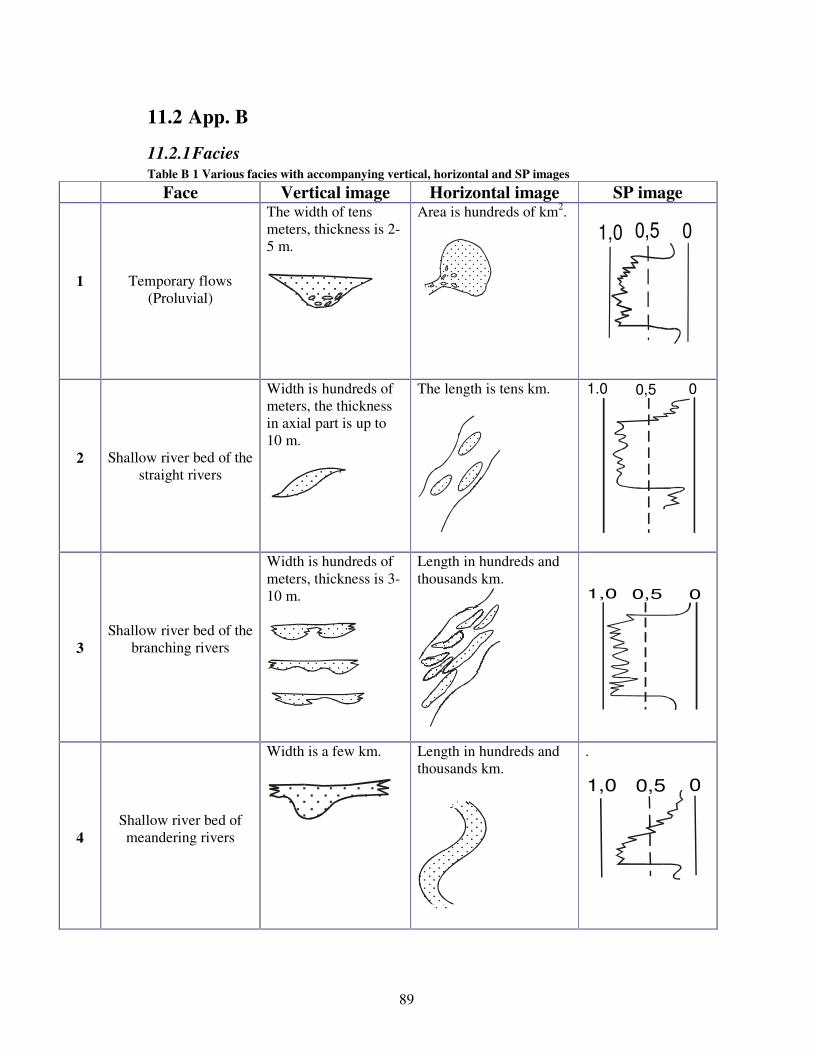
89

11.2 App. B

11.2.1 Facies Table B 1 Various facies with accompanying vertical, horizontal and SP images

Face Vertical image Horizontal image SP image

1

Temporary flows

(Proluvial)

The width of tens

meters, thickness is 2-

5 m.

Area is hundreds of km2.

1,0 0,5 0

2

Shallow river bed of the

straight rivers

Width is hundreds of

meters, the thickness

in axial part is up to

10 m.

The length is tens km.

3

Shallow river bed of the

branching rivers


meters, thickness is 3-

10 m.

Length in hundreds and

thousands km.

1,0 0,5 0

4

Shallow river bed of

meandering rivers

Width is a few km.

Length in hundreds and

thousands km.

.

1,0 0,5 0

1.0 0,5 0

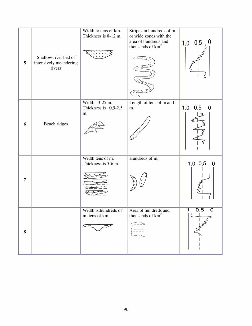
90

5

Shallow river bed of

intensively meandering

rivers

Width to tens of km.

Thickness is 8-12 m.

Stripes in hundreds of m

or wide zones with the

area of hundreds and

thousands of km2.

1,0 0,5 0

6

Beach ridges

Width 3-25 m.

Thickness is 0,5-2,5

m.

Length of tens of m and

m.

1.0 0,5 0

7

Width tens of m.

Thickness is 5-6 m.

Hundreds of m.

1,0 0,5 0

8

Width is:hundreds of

m, tens of km.

Area of hundreds and

thousands of km2

1 00,5

91

9

Floodplain rivers and

lakes

Clays with sublayers

of coal. Width is a few

km.

Tens of km.

10

Underwater slope of

delta

Width is from tens of

m to km. Thickness is

40-70 m.

1,0 0,5 0

11

River dunes (eolian)

Width is 8-15m,

height is

2-3 m.

Length is tens and

hundreds of m.

1,0 0,5 01,0 0,5 0

12

Mouth bar

Width is m and tens of

km. Thickness is up to

10 m.

Area of tens and

hundreds of km2.

1,0 0,5 0

13

Beaches

Width is from m to

km. Height is about 2

m.

Length of tens of km

1.0 0,5 0

92

14

Along beach of

transgressive bars and

near-shore bank

Width is hundreds m,

km.

Height is up to 10m.

Length is tens and

hundreds of km.

1,0 0,5 0

15

Near sea swamps, and

marshes.

Width is km and tens

of km. Thickness is 1-

2 m.

Coaly clay bodies. Area

of tens and hundreds of

km2.

1,0 0,5 0

16

Along –beach

regressive bars and

near-shore banks.

Width is hundreds m,

km.

Height is up to 10m.

Length is tens and

hundreds of km.

1,0 0,5 0

17

Barrier islands

Width m and tens of

m, height is up to 10

m.

Length is tens and

hundreds of km.

1,0 0,5 0

93

18

Lagoons behind bars

during regression of

marine basin

Width is tens of km.

Thickness is up to 4

m.

Area is tens and

hundreds of km2.

Суша

Бар

19

Lagoons behind bars

during transgression of

marine basin

Width is tens of km.

Thickness is up to 4

m.

Area is tens and

hundreds of km2.

Суша

Бар

1,0 0,5 0

20

Gully riptide

Washouts of breaking

currents


m. Thickness is 1-2 m.

Area is tens of km2.

1,0 0,5 0

21

Head parts of breaking

currents

Width is km and tens

of km. Thickness is 2-

5 m.

Area is hundreds of km2.

1,0 0,5 0

94

22

Valley of deltaic

complex

Width is tens and

hundreds of m.

Thickness is 0,5-3,0

м.

Area is tens and

hundreds of km2.

1,0 0,5 0

12

1

23

Sedimentary rocks of

shallow shelf


m and km. Height is

10-40 m. Formed on

the depth of 10-100 m.

Area is tens of km2.

а)

б)

в)

1,0 0,5 0

24

Open sea and large sea

gulfs

Grey and green

montmorillonite.

Width is hundreds and

thousands of

km.Thickness is 50-

200 m.

Hundreds and thousands

of km2

on the sea bottom.

1,0 0,5 0

95

11.3 App. C

11.3.1 Formation Water Resistivity & Salinity data

Table C 1 Resistivity & Salinity data for Well 335R


(mV)

Ref.

depth Rt (ΩΩΩΩ-m) Rm (ΩΩΩΩ-m) Rmf (ΩΩΩΩ-m) Vsp

Essp =

∆∆∆∆Usp/Vsp

(mV)

Rmfeq/Rweq Rmfeq (ΩΩΩΩ-m) Rweq (ΩΩΩΩ-m) Rw (ΩΩΩΩ-

m)

Salinity

(g/L)

A2 – – – – – – – – – – – –

A3 – – – – – – – – – – – –

A4 – – – – – – – – – – – –

A5 -45 1429.0 2.76 3.0 2.4 1 -45 3.5 0.25 0.071 0.0850 37.0

A6 – – – – – – – – – – – –

A7 – – – – – – – – – – – –

A8 -58 1625.4 14.8 3.0 2.4 1 -58 5.2 0.60 0.115 0.1300 22.0

A9 -45 1672.8 14.8 3.0 2.4 1 -45 3.5 0.25 0.071 0.0850 37.0

B1 -38 1722.8 14.0 3.0 2.4 1 -38 3.0 0.20 0.067 0.0750 40.0

B2 -64 1763.2 5.23 3.0 2.4 1 -64 6.0 0.80 0.133 0.1400 20.0

B4 -83 1910.0 4.25 3.0 2.4 1 -83 11.0 2.50 0.227 0.3000 9.0

B5 -83 1984.4 12.1 3.0 2.4 1 -83 11.0 2.50 0.227 0.3000 9.0

B6 -82 2080.8 6.34 3.0 2.4 1 -82 9.0 1.62 0.180 0.2111 13.0

B7 -74 2123.0 2.93 3.0 2.4 1 -74 8.0 1.36 0.170 0.2000 14.0

B8 -89 2215.0 5.53 3.0 2.4 1 -89 12.0 3.00 0.250 0.3500 7.5

B9 -88 2271.4 6.76 3.0 2.4 1 -88 12.0 3.00 0.250 0.3500 7.5

C1 -74 2319.8 7.23 3.0 2.4 1 -74 8.0 1.36 0.170 0.2000 14.0

C2 -92 2346.2 1.31 3.0 2.4 1 -92 12.0 3.00 0.250 0.3500 7.5

C4 -94 2402.0 5.27 3.0 2.4 1 -94 14.0 4.00 0.289 0.4000 6.5

C5 -71 2462.8 11.4 3.0 2.4 1 -71 7.0 1.00 0.143 0.1500 18.5

C6 -89 2485.4 7.44 3.0 2.4 1 -89 12.0 3.00 0.250 0.3500 7.5

C7 -90 2546.6 8.00 3.0 2.4 1 -90 12.0 3.00 0.250 0.3500 7.5

C8 -101 2592.0 3.19 3.0 2.4 1 -101 17.0 6.00 0.353 0.6000 4.0

C9 -102 2622.4 9.1 3.0 2.4 1 -102 17.0 6.00 0.353 0.6000 4.0

96



(mV)

Ref.

depth Rt (ΩΩΩΩ-m) Rm (ΩΩΩΩ-

m)

Rmf (ΩΩΩΩ-m) Vsp Essp =

∆∆∆∆Usp/Vsp

(mV)

Rmfeq/Rweq Rmfeq (ΩΩΩΩ-

m)

Rweq (ΩΩΩΩ-

m)

Rw (ΩΩΩΩ-

m)

Salinity

(g/L)

A2 – – – – – – – – – – – –

A3 – – – – – – – – – – – –

A4 – – – – – – – – – – – –

A5 -60 1414.4 6.73 3.0 2.4 1 -60 5.2 0.60 0.115 0.1300 22.0

A6 – – – – – – – – – – – –

A7 – – – – – – – – – – – –

A8 -75 1614.8 12.1 3.0 2.4 1 -75 8.0 1.36 0.170 0.2000 14.0

A9 -67 1641.0 11.4 3.0 2.4 1 -67 6.0 0.80 0.133 0.1400 20.0

B1 -69 1695.4 94.5 3.0 2.4 1 -69 7.0 1.00 0.143 0.1500 18.5

B2 -65 1765.2 15.9 3.0 2.4 1 -65 6.0 0.80 0.133 0.1400 20.0

B4 -63 1901.0 2.33 3.0 2.4 1 -63 6.0 0.80 0.133 0.1400 20.0

B5 -93 1982.6 10.7 3.0 2.4 1 -93 14.0 4.00 0.289 0.4000 6.5

B6 -86 2047.0 3.94 3.0 2.4 1 -86 11.0 2.50 0.227 0.3000 9.0

B7 -88 2089.2 2.96 3.0 2.4 1 -88 12.0 3.00 0.250 0.3500 7.5

B8 -90 2193.2 2.23 3.0 2.4 1 -90 12.0 3.00 0.250 0.3500 7.5

B9 -101 2238.6 5.11 3.0 2.4 1 -101 17.0 6.00 0.353 0.6000 4.0

C1 -88 2287.0 3.76 3.0 2.4 1 -88 12.0 3.00 0.250 0.3500 7.5

C2 -86 2312.8 1.12 3.0 2.4 1 -86 11.0 2.50 0.227 0.3000 9.0

C4 -94 2371.2 5.48 3.0 2.4 1 -94 14.0 4.00 0.289 0.4000 6.5

C5 -57 2428.8 7.26 3.0 2.4 1 -57 4.6 0.50 0.109 0.1200 25.0

C6 -96 2464.6 3.41 3.0 2.4 1 -96 14.0 4.00 0.289 0.4000 6.5

C7 -87 2505.0 9.95 3.0 2.4 1 -87 11.0 2.50 0.227 0.3000 9.0

C8 -95 2540.4 4.44 3.0 2.4 1 -95 14.0 4.00 0.289 0.4000 6.5

C9 -105 2580.2 4.69 3.0 2.4 1 -105 18.00 7.00 0.389 0.8000 3.0

97



(mV)

Ref.


m)


∆∆∆∆Usp/Vsp

(mV)

Rmfeq/Rweq Rmfeq (ΩΩΩΩ-m) Rweq (ΩΩΩΩ-

m)

Rw (ΩΩΩΩ-

m)

Salinity

(g/L)

A2 – – – – – – – – – – – –

A3 – – – – – – – – – – – –

A4 – – – – – – – – – – – –

A5 -53 1404.4 13.9 3.0 2.4 1 -53 4.6 0.50 0.109 0.1200 25.0

A6 -52 1456.4 4.00 3.0 2.4 1 -52 4.0 0.35 0.088 0.1000 30.0

A7 -58 1542.0 6.5 3.0 2.4 1 -58 5.2 0.60 0.115 0.1300 22.0

A8 -61 1606.0 5.83 3.0 2.4 1 -61 5.2 0.60 0.115 0.1300 22.0

A9 -60 1641.8 8.71 3.0 2.4 1 -60 5.2 0.60 0.115 0.1300 22.0

B1 -62 1693.0 3.41 3.0 2.4 1 -62 5.2 0.60 0.115 0.1300 22.0

B2 -62 1764.4 12.0 3.0 2.4 1 -62 5.2 0.60 0.115 0.1300 22.0

B4 -70 1882.0 9.04 3.0 2.4 1 -70 7.0 1.00 0.143 0.1500 18.5

B5 -78 1996.2 24.5 3.0 2.4 1 -78 9.0 1.62 0.180 0.2100 13.0

B6 -77 2043.8 7.92 3.0 2.4 1 -77 8.0 1.36 0.170 0.2000 14.0

B7 -57 2085.8 5.58 3.0 2.4 1 -57 4.6 0.50 0.109 0.1200 25.0

B8 -89 2176.4 3.83 3.0 2.4 1 -89 12.0 3.00 0.250 0.3500 7.5

B9 -87 2228.0 10.7 3.0 2.4 1 -87 11.0 2.50 0.227 0.3000 9.0

C1 -82 2296.0 3.21 3.0 2.4 1 -82 9.0 1.62 0.180 0.2100 13.0

C2 -79 2328.2 4.0 3.0 2.4 1 -79 9.0 1.62 0.180 0.2100 13.0

C4 -88 2366.4 7.17 3.0 2.4 1 -88 12.0 3.00 0.250 0.3500 7.5

C5 -69 2429.8 4.46 3.0 2.4 1 -69 7.0 1.00 0.143 0.1500 18.5

C6 -84 2441.6 3.21 3.0 2.4 1 -84 11.0 2.50 0.227 0.3000 9.0

C7 -79 2514.4 9.5 3.0 2.4 1 -79 9.0 1.62 0.180 0.2100 13.0

C8 -74 2551.4 8.29 3.0 2.4 1 -74 8.0 1.36 0.170 0.2000 14.0

C9 -83 2585.2 6.0 3.0 2.4 1 -83 11.0 2.50 0.227 0.3000 9.0

98



(mV)

Ref.


m)


∆∆∆∆Usp/Vsp

(mV)


m)

Rw (ΩΩΩΩ-

m)

Salinity

(g/L)

A2 -44 1150.6 2.38 3.0 2.4 1 -44 3.5 0.25 0.071 0.0850 37.0

A3 -40 1183.0 2.57 3.0 2.4 1 -40 3.0 0.20 0.067 0.0750 40.0

A4 -41 1333.0 2.22 3.0 2.4 1 -41 3.0 0.20 0.067 0.0750 40.0

A5 -53 1429.4 4.19 3.0 2.4 1 -53 4.6 0.50 0.109 0.1200 25.0

A6 -51 1478.0 2.36 3.0 2.4 1 -51 4.0 0.35 0.088 0.1000 30.0

A7 -51 1569.0 2.22 3.0 2.4 1 -51 4.0 0.35 0.088 0.1000 30.0

A8 -52 1630.2 2.92 3.0 2.4 1 -52 4.0 0.35 0.088 0.1000 30.0

A9 -48 1669.0 3.56 3.0 2.4 1 -48 4.0 0.35 0.088 0.1000 30.0

B1 -51 1695.4 2.36 3.0 2.4 1 -51 4.0 0.35 0.088 0.1000 30.0

B2 -60 1756.2 10.8 3.0 2.4 1 -60 5.2 0.60 0.115 0.1300 22.0

B4 -62 1879.0 10.7 3.0 2.4 1 -62 5.2 0.60 0.115 0.1300 22.0

B5 -69 2000.4 1.71 3.0 2.4 1 -69 7.0 1.00 0.143 0.1500 18.5

B6 -71 2049.0 4.0 3.0 2.4 1 -71 7.0 1.00 0.143 0.1500 18.5

B7 -68 2114.6 4.35 3.0 2.4 1 -68 7.0 1.00 0.143 0.1500 18.5

B8 -70 2188.2 4.67 3.0 2.4 1 -70 7.0 1.00 0.143 0.1500 18.5

B9 -74 2253.4 4.5 3.0 2.4 1 -74 8.0 1.36 0.170 0.2000 14.0

C1 -70 2295.0 1.12 3.0 2.4 1 -70 7.0 1.00 0.143 0.1500 18.5

C2 -76 2333.4 3.94 3.0 2.4 1 -76 8.0 1.36 0.170 0.2000 14.0

C4 -74 2387.0 5.19 3.0 2.4 1 -74 8.0 1.36 0.170 0.2000 14.0

C5 -69 2435.4 4.46 3.0 2.4 1 -69 7.0 1.00 0.143 0.1500 18.5

C6 -68 2474.6 7.71 3.0 2.4 1 -68 7.0 1.00 0.143 0.1500 18.5

C7 -77 2523.0 9.99 3.0 2.4 1 -77 8.0 1.36 0.170 0.2000 14.0

C8 -69 2556.4 9.71 3.0 2.4 1 -69 7.0 1.00 0.143 0.1500 18.5

C9 -73 2588.6 16.8 3.0 2.4 1 -73 8.0 1.36 0.170 0.2000 14.0

99



(mV)

Ref.


m)


∆∆∆∆Usp/Vsp

(mV)


m)

Rw (ΩΩΩΩ-

m)

Salinity

(g/L)

A2 -44 1156.8 3.82 3.0 2.4 1 -44 3.5 0.25 0.071 0.0850 37.0

A3 -45 1178.6 3.02 3.0 2.4 1 -45 3.5 0.25 0.071 0.0850 37.0

A4 -52 1345.0 3.06 3.0 2.4 1 -52 4.0 0.35 0.088 0.1000 30.0

A5 -59 1422.2 4.44 3.0 2.4 1 -59 5.2 0.60 0.115 0.1300 22.0

A6 -55 1478.6 3.56* 3.0 2.4 1 -55 4.6 0.50 0.109 0.1200 25.0

A7 -60 1546.2 2.68* 3.0 2.4 1 -60 5.2 0.60 0.115 0.1300 22.0

A8 -62 1617.9 4.78 3.0 2.4 1 -62 5.2 0.60 0.115 0.1300 22.0

A9 -53 1654.6 3.02 3.0 2.4 1 -53 4.6 0.50 0.109 0.1200 25.0

B1 -62 1692.0 3.44 3.0 2.4 1 -62 5.2 0.60 0.115 0.1300 22.0

B2 -73 1764.0 1.8 3.0 2.4 1 -73 8.0 1.36 0.170 0.2000 14.0

B4 -75 1882.2 9.27 3.0 2.4 1 -75 8.0 1.36 0.170 0.2000 14.0

B5 -87 1976.3 11.3/.8 3.0 2.4 1 -87 11.0 2.50 0.227 0.3000 9.0

B6 -80 2046.9 8.43 3.0 2.4 1 -80 9.0 1.62 0.180 0.2100 13.0

B7 -89 2113.8 2.72 3.0 2.4 1 -89 12.0 3.00 0.250 0.3500 7.5

B8 -95 2199.0 3.52 3.0 2.4 1 -95 14.0 4.00 0.289 0.4000 6.5

B9 – – – – – – – – – – – –

C1 -86 2291.5 3.35 3.0 2.4 1 -86 11.0 2.50 0.227 0.3000 9.0

C2 -100 2334.5 4.02 3.0 2.4 1 -100 17.0 6.00 0.353 0.6000 4.0

C4 -100 2400.0 0.504 3.0 2.4 1 -100 17.0 6.00 0.353 0.6000 4.0

C5 -100 2440.0 1.84 3.0 2.4 1 -100 17.0 6.00 0.353 0.6000 4.0

C6 -99 2466.7 3.23 3.0 2.4 1 -99 17.0 6.00 0.353 0.6000 4.0

C7 -103 2519.9 4.19 3.0 2.4 1 -103 18.00 7.00 0.389 0.8000 3.0

C8 -75 2556.8 8.22 3.0 2.4 1 -75 8.0 1.36 0.170 0.2000 14.0

C9 – – – – – – – – – – – –

100

11.4 App. D

11.4.1 Permeability data Table D 1 Permeability data for wells 335R, 360R, 333R, 313R and 338R

335R Layer φφφφ k

A2 – –

A3 – –

A4 – –

A5 0.448 14.993

A6 – –

A7 – –

A8 0.093 1.418

A9 0.288 7.728

B1 0.323 9.179

B2 0.168 3.443

B4 0.095 1.464

B5 0.092 1.395

B6 0.091 1.373

B7 0.238 5.805

B8 0.093 1.418

B9 0.092 1.395

C1 0.397 12.507

C2 0.134 2.453

C4 0.092 1.395

C5 0.159 3.170

C6 0.093 1.418

C7 0.140 2.619

C8 0.185 3.979

C9 0.094 1.441


A2 – –

A3 – –

A4 – –

A5 0.117 2.001

A6 – –

A7 – –

A8 0.075 1.027

A9 0.108 1.775

B1 0.070 0.926

B2 0.101 1.605

B4 0.248 6.175

B5 0.060 0.735

B6 0.205 4.641

B7 0.219 5.124

B8 0.234 5.660

B9 0.118 2.027

C1 0.218 5.089

C2 0.229 5.479

C4 0.141 2.647

C5 0.168 3.443

C6 0.219 5.124

C7 0.101 1.605

C8 0.292 7.889

C9 0.121 2.104


A2 – –

A3 – –

A4 – –

A5 0.102 1.629

A6 0.152 2.963

A7 0.062 0.772

A8 0.183 3.914

A9 0.171 3.536

B1 0.250 6.250

B2 0.121 2.104

B4 0.211 4.846

B5 0.064 0.810

B6 0.126 2.236

B7 0.227 5.408

B8 0.208 4.743

B9 0.073 0.986

C1 0.208 4.743

C2 0.246 6.101

C4 0.154 3.022

C5 0.218 5.089

C6 0.261 6.667

C7 0.111 1.849

C8 0.140 2.619

C9 0.119 2.053


A2 0.328 9.392

A3 0.318 8.966

A4 0.304 8.381

A5 0.173 3.598

A6 0.244 6.026

A7 0.217 5.054

A8 0.283 7.527

A9 0.292 7.889

B1 0.218 5.089

B2 0.168 3.443

B4 0.070 0.926

B5 0.213 4.915

B6 0.132 2.398

B7 0.264 6.782

B8 0.119 2.053

B9 0.051 0.576

C1 0.141 2.647

C2 0.116 1.975

C4 0.128 2.290

C5 0.429 14.049

C6 0.125 2.210

C7 0.076 1.048

C8 0.149 2.876

C9 0.100 1.581

101


A2 0.465 15.854

A3 0.516 18.533

A4 0.492 17.255

A5 0.193 4.239

A6 0.454 15.295

A7 0.382 11.805

A8 0.347 10.220

A9 0.330 9.479

B1 0.275 7.211

B2 0.296 8.052

B4 0.081 1.153

B5 0.059 0.717

B6 0.095 1.464

B7 0.279 7.368

B8 0.203 4.573

B9 – –

C1 0.192 4.207

C2 0.175 3.660

C4 0.284 7.567

C5 0.293 7.930

C6 0.258 6.552

C7 0.254 6.401

C8 0.136 2.508

C9 – –

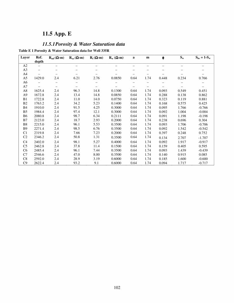
102

11.5 App. E

11.5.1 Porosity & Water Saturation data

Table E 1 Porosity & Water Saturation data for Well 335R

Layer Ref.


A2 – – – – – – – – – –

A3 – – – – – – – – – –

A4 – – – – – – – – – –

A5 1429.0 2.4 6.21 2.76 0.0850 0.64 1.74 0.448 0.234 0.766

A6 – – – – – – – – – –

A7 – – – – – – – – – –

A8 1625.4 2.4 96.3 14.8 0.1300 0.64 1.74 0.093 0.549 0.451

A9 1672.8 2.4 13.4 14.8 0.0850 0.64 1.74 0.288 0.138 0.862

B1 1722.8 2.4 11.0 14.0 0.0750 0.64 1.74 0.323 0.119 0.881

B2 1763.2 2.4 34.2 5.23 0.1400 0.64 1.74 0.168 0.575 0.425

B4 1910.0 2.4 91.5 4.25 0.3000 0.64 1.74 0.095 1.766 -0.766

B5 1984.4 2.4 97.4 12.1 0.3000 0.64 1.74 0.092 1.004 -0.004

B6 2080.8 2.4 98.7 6.34 0.2111 0.64 1.74 0.091 1.198 -0.198

B7 2123.0 2.4 18.7 2.93 0.2000 0.64 1.74 0.238 0.696 0.304

B8 2215.0 2.4 96.1 5.53 0.3500 0.64 1.74 0.093 1.706 -0.706

B9 2271.4 2.4 98.5 6.76 0.3500 0.64 1.74 0.092 1.542 -0.542

C1 2319.8 2.4 7.66 7.23 0.2000 0.64 1.74 0.397 0.248 0.752

C2 2346.2 2.4 50.8 1.31 0.3500 0.64 1.74 0.134 2.707 -1.707

C4 2402.0 2.4 98.1 5.27 0.4000 0.64 1.74 0.092 1.917 -0.917

C5 2462.8 2.4 37.8 11.4 0.1500 0.64 1.74 0.159 0.405 0.595

C6 2485.4 2.4 96.1 7.44 0.3500 0.64 1.74 0.093 1.439 -0.439

C7 2546.6 2.4 47.0 8.00 0.3500 0.64 1.74 0.140 0.915 0.085

C8 2592.0 2.4 28.9 3.19 0.6000 0.64 1.74 0.185 1.600 -0.600

C9 2622.4 2.4 93.2 9.1 0.6000 0.64 1.74 0.094 1.717 -0.717

103

Layer Ref.


A2 – – – – – – – – – –

A3 – – – – – – – – – –

A4 – – – – – – – – – –

A5 1414.4 2.4 64.2 6.73 0.1300 0.64 1.74 0.117 0.684 0.316

A6 – – – – – – – – – –

A7 – – – – – – – – – –

A8 1614.8 2.4 138 12.1 0.2000 0.64 1.74 0.075 0.971 0.029

A9 1641.0 2.4 74.1 11.4 0.1400 0.64 1.74 0.108 0.573 0.427

B1 1695.4 2.4 158 94.5 0.150 0.64 1.74 0.070 0.273 0.727

B2 1765.2 2.4 82.6 15.9 0.1400 0.64 1.74 0.101 0.504 0.496

B4 1901.0 2.4 17.4 2.33 0.1400 0.64 1.74 0.248 0.620 0.380

B5 1982.6 2.4 207 10.7 0.4000 0.64 1.74 0.060 1.960 -0.960

B6 2047.0 2.4 24.3 3.94 0.3000 0.64 1.74 0.205 0.861 0.139

B7 2089.2 2.4 21.6 2.96 0.3500 0.64 1.74 0.219 1.036 -0.036

B8 2193.2 2.4 19.3 2.23 0.3500 0.64 1.74 0.234 1.143 -0.143

B9 2238.6 2.4 63.1 5.11 0.6000 0.64 1.74 0.118 1.911 -0.911

C1 2287.0 2.4 21.8 3.76 0.3500 0.64 1.74 0.218 0.908 0.092

C2 2312.8 2.4 19.9 1.12 0.3000 0.64 1.74 0.229 1.582 -0.582

C4 2371.2 2.4 46.6 5.48 0.4000 0.64 1.74 0.141 1.222 -0.222

C5 2428.8 2.4 34.1 7.26 0.1200 0.64 1.74 0.168 0.435 0.565

C6 2464.6 2.4 21.5 3.41 0.4000 0.64 1.74 0.219 1.029 -0.029

C7 2505.0 2.4 82.3 9.95 0.3000 0.64 1.74 0.101 1.019 -0.019

C8 2540.4 2.4 13.1 4.44 0.4000 0.64 1.74 0.292 0.665 0.335

C9 2580.2 2.4 61.0 4.69 0.8000 0.64 1.74 0.121 2.323 -1.323


104


Layer Ref.

depth Rmf (ΩΩΩΩ-m) Rxo (ΩΩΩΩ-m) Rt (ΩΩΩΩ-m) Rw (ΩΩΩΩ-

m)

a m φφφφ Sw Shc = 1-Sw

A2 – – – – – – – – – –

A3 – – – – – – – – – –

A4 – – – – – – – – – –

A5 1404.4 2.4 81.8 13.9 0.1200 0.64 1.74 0.102 0.495 0.505

A6 1456.4 2.4 40.9 4.00 0.1000 0.64 1.74 0.152 0.612 0.388

A7 1542.0 2.4 196 6.5 0.1300 0.64 1.74 0.062 1.326 -0.326

A8 1606.0 2.4 29.5 5.83 0.1300 0.64 1.74 0.183 0.475 0.525

A9 1641.8 2.4 33.3 8.71 0.1300 0.64 1.74 0.171 0.405 0.595

B1 1693.0 2.4 17.1 3.41 0.1300 0.64 1.74 0.250 0.473 0.527

B2 1764.4 2.4 60.4 12.0 0.1300 0.64 1.74 0.121 0.474 0.526

B4 1882.0 2.4 23 9.04 0.1500 0.64 1.74 0.211 0.348 0.652

B5 1996.2 2.4 183 24.5 0.2100 0.64 1.74 0.064 0.783 0.217

B6 2043.8 2.4 56.2 7.92 0.2000 0.64 1.74 0.126 0.739 0.261

B7 2085.8 2.4 20.3 5.58 0.1200 0.64 1.74 0.227 0.376 0.624

B8 2176.4 2.4 23.7 3.83 0.3500 0.64 1.74 0.208 0.943 0.057

B9 2228.0 2.4 145 10.7 0.3000 0.64 1.74 0.073 1.354 -0.354

C1 2296.0 2.4 23.7 3.21 0.2100 0.64 1.74 0.208 0.778 0.222

C2 2328.2 2.4 17.6 4.0 0.2100 0.64 1.74 0.246 0.578 0.422

C4 2366.4 2.4 39.8 7.17 0.3500 0.64 1.74 0.154 0.886 0.114

C5 2429.8 2.4 21.8 4.46 0.1500 0.64 1.74 0.218 0.506 0.494

C6 2441.6 2.4 15.9 3.21 0.3000 0.64 1.74 0.261 0.759 0.241

C7 2514.4 2.4 70.3 9.5 0.2100 0.64 1.74 0.111 0.779 0.221

C8 2551.4 2.4 47.2 8.29 0.2000 0.64 1.74 0.140 0.651 0.349

C9 2585.2 2.4 62.5 6.0 0.3000 0.64 1.74 0.119 1.164 -0.164

105

Layer Ref.


A2 1150.6 2.4 10.7 2.38 0.0850 0.64 1.74 0.328 0.348 0.652

A3 1183.0 2.4 11.3 2.57 0.0750 0.64 1.74 0.318 0.320 0.680

A4 1333.0 2.4 12.2 2.22 0.0750 0.64 1.74 0.304 0.363 0.637

A5 1429.4 2.4 32.4 4.19 0.1200 0.64 1.74 0.173 0.579 0.421

A6 1478.0 2.4 17.9 2.36 0.1000 0.64 1.74 0.244 0.516 0.484

A7 1569.0 2.4 22 2.22 0.1000 0.64 1.74 0.217 0.601 0.399

A8 1630.2 2.4 13.8 2.92 0.1000 0.64 1.74 0.283 0.393 0.607

A9 1669.0 2.4 13.1 3.56 0.1000 0.64 1.74 0.292 0.340 0.660

B1 1695.4 2.4 21.8 2.36 0.1000 0.64 1.74 0.218 0.578 0.422

B2 1756.2 2.4 34.4 10.8 0.1300 0.64 1.74 0.168 0.364 0.636

B4 1879.0 2.4 157 10.7 0.1300 0.64 1.74 0.070 0.876 0.124

B5 2000.4 2.4 22.7 1.71 0.1500 0.64 1.74 0.213 0.898 0.102

B6 2049.0 2.4 52.1 4.0 0.1500 0.64 1.74 0.132 0.888 0.112

B7 2114.6 2.4 15.6 4.35 0.1500 0.64 1.74 0.264 0.423 0.577

B8 2188.2 2.4 62.2 4.67 0.1500 0.64 1.74 0.119 0.900 0.100

B9 2253.4 2.4 273 4.5 0.2000 0.64 1.74 0.051 2.538 -1.538

C1 2295.0 2.4 46.7 1.12 0.1500 0.64 1.74 0.141 1.734 -0.734

C2 2333.4 2.4 65.4 3.94 0.2000 0.64 1.74 0.116 1.205 -0.205

C4 2387.0 2.4 55 5.19 0.2000 0.64 1.74 0.128 0.931 0.069

C5 2435.4 2.4 6.71 4.46 0.1500 0.64 1.74 0.429 0.257 0.743

C6 2474.6 2.4 57.6 7.71 0.1500 0.64 1.74 0.125 0.646 0.354

C7 2523.0 2.4 135 9.99 0.2000 0.64 1.74 0.076 1.071 -0.071

C8 2556.4 2.4 42.3 9.71 0.1500 0.64 1.74 0.149 0.473 0.527

C9 2588.6 2.4 85 16.8 0.2000 0.64 1.74 0.100 0.609 0.391


106


Layer Ref.

depth Rmf (ΩΩΩΩ-m) Rxo (ΩΩΩΩ-

m)

Rt (ΩΩΩΩ-m) Rw (ΩΩΩΩ-

m)

a m φφφφ Sw Shc = 1-Sw

A2 1156.8 2.4 5.83 3.82 0.0850 0.64 1.74 0.465 0.187 0.813

A3 1178.6 2.4 4.85 3.02 0.0850 0.64 1.74 0.516 0.193 0.807

A4 1345.0 2.4 5.27 3.06 0.1000 0.64 1.74 0.492 0.220 0.780

A5 1422.2 2.4 27 4.44 0.1300 0.64 1.74 0.193 0.528 0.472

A6 1478.6 2.4 6.08 3.56* 0.1200 0.64 1.74 0.454 0.243 0.757

A7 1546.2 2.4 8.21 2.68* 0.1300 0.64 1.74 0.382 0.356 0.644

A8 1617.9 2.4 9.7 4.78 0.1300 0.64 1.74 0.347 0.281 0.719

A9 1654.6 2.4 10.6 3.02 0.1200 0.64 1.74 0.330 0.368 0.632

B1 1692.0 2.4 14.5 3.44 0.1300 0.64 1.74 0.275 0.428 0.572

B2 1764.0 2.4 12.8 1.8 0.2000 0.64 1.74 0.296 0.740 0.260

B4 1882.2 2.4 122 9.27 0.2000 0.64 1.74 0.081 1.054 -0.054

B5 1976.3 2.4 213/268 11.3/.8 0.3000 0.64 1.74 0.059 1.636 -0.636

B6 2046.9 2.4 92.5 8.43 0.2100 0.64 1.74 0.095 0.977 0.023

B7 2113.8 2.4 14.2 2.72 0.3500 0.64 1.74 0.279 0.855 0.145

B8 2199.0 2.4 24.6 3.52 0.4000 0.64 1.74 0.203 1.092 -0.092

B9 – – – – – – – – – –

C1 2291.5 2.4 27.2 3.35 0.3000 0.64 1.74 0.192 1.009 -0.009

C2 2334.5 2.4 31.9 4.02 0.6000 0.64 1.74 0.175 1.482 -0.482

C4 2400.0 2.4 13.7 0.504 0.6000 0.64 1.74 0.284 3.008 -2.008

C5 2440.0 2.4 13 1.84 0.6000 0.64 1.74 0.293 1.387 -0.387

C6 2466.7 2.4 16.2 3.23 0.6000 0.64 1.74 0.258 1.139 -0.139

C7 2519.9 2.4 16.7 4.19 0.8000 0.64 1.74 0.254 1.177 -0.177

C8 2556.8 2.4 49.7 8.22 0.2000 0.64 1.74 0.136 0.674 0.326

C9 – – – – – – – – – –

Stephanie Otema Adu Master Thesis June 6, 2011

Documents

Transcript of Stephanie Otema Adu Master Thesis June 6, 2011