Step 5: Conduct Analysis The CCA Algorithm

1

Model Parameterization:

Step 5: Conduct Analysis

P Dropped species with fewer than 5 occurrences

P Log-transformed species abundances

P Row-normalized species’ log abundances (chord distance)

P Selected smallest “best”subset of variables from eachset of independent variables

P Chose RDA (in combo withchord distance)

2

The CCA Algorithm

P Gradients are assumed tobe linear combinations ofthe environmentalvariables.

P Key assumption is that ofunimodal speciesdistributions alongenvironmental gradients.

CCA estimates species optima,regression coefficients, and sitescores using a Gaussianweighted-averaging modelcombined with regression.

Assign arbitraryweights to samples

Compute species scores asweighted averages

Rescale (standardize)sample scores

Compute sample scores asweighted averages

Subsequent axes computedfrom residuals

Regress sample scores on environmentalvariables and assign new sample scoresas the predicted values from regression

3

Step 6: Interpret Results

P Effectiveness of the Constrained Ordination

< Total inertia, eigenvalues, percent variance explained,significance tests, species-environment correlation,cumulative species/sample fit.

P Interpreting the Constrained Ordination

< Canonical coefficients, inter-set and intra-setcorrelations, biplot scores.

< The Triplot: sample vs species scaling, centroid rulevs biplot rule, general interpretation.

< Interpreting species-environment relationships.

4

Effectiveness of the Constrained Ordination

Total inertiaP Sum of the eigenvalues; total

“variance” in the speciesdata, some of which isaccounted for by theenvironmental constraints.

EigenvaluesP Variance in the community

matrix attributed to aparticular axis; measure ofimportance of the ordinationaxis.

5

P Proportion of speciesvariance (total inertia)explained by each axis.Computed aseigenvalue/total inertia(reported as cumulative %).

Percent “variance” of species dataP For ecological data the

percentage of explained varianceis usually low; often ~ 10%. Notto worry, as it is an inherentfeature of data with a strongpresence/absence aspect.


6

Significance TestsP Monte Carlo global

permutation tests ofsignificance of canonicalaxes.

P Test based on 1st canonical axis has maximum poweragainst the alternative hypothesis that there is a singledominating gradient that determines the relation betweenthe species and environment.


7

Scores for Sites and Species

P Ordination scores (coordinates on ordination axes) givenfor each site (sample) and each species. Two sets ofscores are produced for sites (samples):

< Linear combination (LC) scores – linear combinations ofthe independent variables. LC scores are inenvironmental space, each axis formed by linearcombinations of environmental variables.

< Weighted averages (WA) scores – weighted averages (sums)of the species scores that are as simimlar to LC scoresas possible. WA scores are in species space.

LC scores show were the site should be; theWA scores show where the site is.


8

LC scores (samples) WA scores (samples)


9

LC versus WA Scores

P Longstanding debate (confusion) over whether to use LCor WA scores.

P LC scores are very sensitive to noise in the environmentaldata, whereas the WA scores are much more stable, beinglargely determined by the species data rather than being adirect projection in environmental space.

“Use of LC scores will misrepresent the observedcommunity relationships unless the environmental dataare both noiseless and meaningful.... CCA (RDA) withLC scores is inappropriate where the objective is todescribe community structure.” (McCune)


10

Species-environmental correlationsP The multiple correlation coefficient of the final regression.

Correlation between site scores computed as weightedaverages of species scores (WA’s) and site scores computedas linear combinations of environmental variables (LC’s);measures how well the extracted variation in communitycomposition can be explained by environmental variables.

“This is a bad measure of goodness of ordination,because it is sensitive to extreme scores (likecorrelations are), and very sensitive to overfitting orusing too many constraints.” (Oksanen)


11

P Ordination diagnostic to find outwhich species/samples are ill-represented in the ordination.

< % variance (inertia) explainedby selected axes.

Goodness-of-Fit for Species/Samples

Plot species with >10% explained


12

Interpreting the Constrained Ordination

Canonical Coefficients

P Regression coefficients of the linear combinations ofenvironmental variables that define the ordination axes;they are eigenvector coefficients and not very useful forinterpretation.

Unstandardizedcoefficients

Standardizedcoefficients

13

IntRA-set Correlation (structure) Coefficients

P Correlations between sample scores derived as linearcombinations of environmental variables (LC scores) andenvironmental variables (i.e., loadings); they are related tothe canonical coefficients but differ in several importantaspects.


14

P Both canonical coefficients and IntRA-set correlationsrelate to the rate of change in community compositionper unit change in the corresponding environmentalvariable – but for canonical coefficients it is assumed thatother environmental variables are being held constant,while for IntRA-set correlations other environmentalvariables are assumed to covary as they do in the dataset.

P When variables are intercorrelated canonical coefficientsbecome unstable – the multicollinearity problem;however, IntRA-set correlations are not effected.



15

P Canonical coefficients and IntRA-set correlationsindicate which environmental variables are moreinfluential in structuring the ordination, but cannot beviewed as an independent measure of the strength ofrelationship between communities and environmentalvariables.

P Probably only meaningful if the site scores are derived asLC scores (which is generally not recommended).

“They have all the problems of correlations, like beingsensitive to extreme values, and they focus on therelationship between single constraints and single axesinstead of multivariate analysis.” (Oksanen)



16

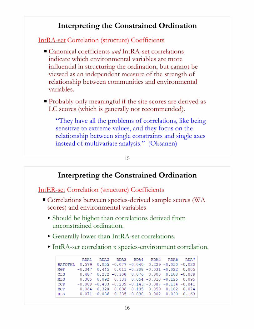
P Correlations between species-derived sample scores (WAscores) and environmental variables.

< Should be higher than correlations derived fromunconstrained ordination.

< Generally lower than IntRA-set correlations.

< IntRA-set correlation x species-environment correlation.

IntER-set Correlation (structure) Coefficients


17

P Like IntRA-set correlations, they do not become unstablewhen the environmental variables are strongly correlatedwith each other (multicollinear).

P Probably only meaningful if the site scores are derived asWA scores (which is generally recommended).

IntER-set Correlation (structure) Coefficients

“They have all the problems of correlations, like beingsensitive to extreme values, and they focus on therelationship between single constraints and single axesinstead of multivariate analysis.” (Oksanen)


18

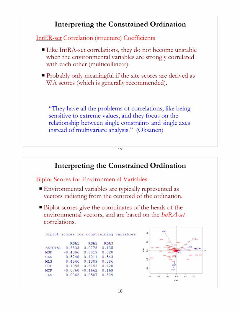
P Environmental variables are typically represented asvectors radiating from the centroid of the ordination.

P Biplot scores give the coordinates of the heads of theenvironmental vectors, and are based on the IntRA-setcorrelations.

Biplot Scores for Environmental Variables


19

The Canonical Triplot

P The triplot displays themajor patterns in the speciesdata with respect to theenvironmental variables.

Tri =(1) Samples(2) Species(3) Environment

P But there are a number ofways to scale the triplotwhich affect the exactquantitative interpretationof the relationships shown.

20

P Optimally displays inter-sample relationships.

P Variance of sample scoreson each axis reflects theimportance of the axis asmeasured by theeigenvalue, whereas thevariance of the speciesscores along the axes areequal.

Sample Scaling


21

P Optimally displays inter-species relationships.

P Variance of species scores oneach axis reflects theimportance of the axis asmeasured by the eigenvalue,whereas the variance of thesample scores along the axesare equal.

Species Scaling

Generally the preferred scaling


22

P Way of interpretingordination diagrams inunimodal methods (CCA).

P Each species' point is at thecentroid (weighted average)of the sample points where itoccurs (i.e., center of itsniche); the samples thatcontain a particular speciesare scattered around thatspecies' point in the diagram.

The Centroid Principle

Species-Hill’s Scaling


23

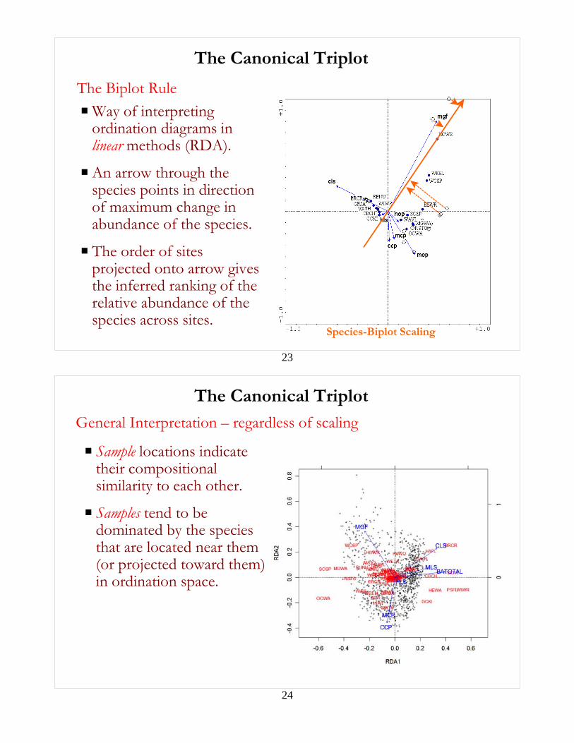
The Biplot Rule

Species-Biplot Scaling

P Way of interpretingordination diagrams inlinear methods (RDA).

P An arrow through thespecies points in directionof maximum change inabundance of the species.

P The order of sitesprojected onto arrow givesthe inferred ranking of therelative abundance of thespecies across sites.


24


P Sample locations indicatetheir compositionalsimilarity to each other.

P Samples tend to bedominated by the speciesthat are located near them(or projected toward them)in ordination space.

General Interpretation – regardless of scaling

25


P Species locations indicatetheir distributionalsimilarity to each other.

P Species tend to be mostpresent and abundant inthe sites that are locatednear them (or in thedirection of theirprojection) in ordinationspace.


26


P Length of environmentalvector indicates itsimportance to theordination.

P Direction of the vectorindicates its correlationwith each of the axes.

P Angles between vectorsindicate the correlationbetween the environmentalvariables themselves.


27


P In unimodal model (CCA),perpendiculars drawn fromspecies to environmentalarrow gives approximateranking of species responseto that variable, andwhether species has higher-than-average or lower-thanaverage optimum on thatenvironmental variable.

Higher-than-average

Lower-than-average


28


P In linear model (RDA),direction of arrow drawnfrom orgin to species andenvironmental arrow givesapproximate relationshipbetween species andenvironmental variable; i.e.,whether species haspositive or negativerelationship with thatenvironmental variable.

Positivecorrelation

Negativecorrelation


29


P Perpendiculars drawn fromsamples to environmentalarrows gives approximateranking of sample valuesfor that environmentalvariable.

P And whether a sample has ahigher-than-average orlower-than-average valueon that environmentalvariable.

Higher-than-average

Lower-than-average


30

P It is more natural torepresent nominalenvironmental variables bypoints instead of arrows.

P The points are located at thecentroid of sites that belongto that class.

P Classes containing sites withhigh values for a species willtend to lie close to thatspecies point.

Nominal Environmental Variables


31

Don’t worry; focuson relationships


Samples-scaling Species-scaling

32

P Chi-square distance amongsamples preserved(approximates unimodalspecies responses).

P Rare species are givendisproportionate weight inthe analysis.

P Unequal weighting of sites inthe regression (equal to sitetotals).

Major Differences Between RDA and CCA

P Euclidean distance amongsamples preserved(appropriate with linearspecies respones and canapproximate unimodalresponses with appropriatedata transformations).

P Rare species are not given highweight in the analysis.

P Equal weighting of sites in theregression.

CCA/dCCA RDA

33

P Species-environmentcorrelation equals thecorrelation between the sitescores that are weightedaverages of the species scores(WA’s) and the site scoresthat are a linear combinationof the environmentalvariables (LC’s).

P Ordination diagram can beinterpreted using the centroidprinciple.

Major Differences Between RDA and CCA

P Species-environmentcorrelation equals thecorrelation between the sitescores that are weighted sumsof the species scores (WA’s)and the site scores that are alinear combination of theenvironmental variables(LC’s).

P Ordination diagram can beinterpreted using the biplotrule.

CCA/dCCA RDA

34

Usefulness of Constrained Ordination

Displaying Interpretable Relationships

P Constrained ordination (aswith any ordination) isultimately about portrayingmeaningful species-environment relationships.

35




36




37

Multivariate Regression Trees (MRT)

P Nonparametric procedure useful for exploration,description, and prediction of species-environmentrelationships (De’ath 2002).

P Natural extension of Univariate Regression Trees (URT):with the univariate response of URT being replacedby a multivariate response.

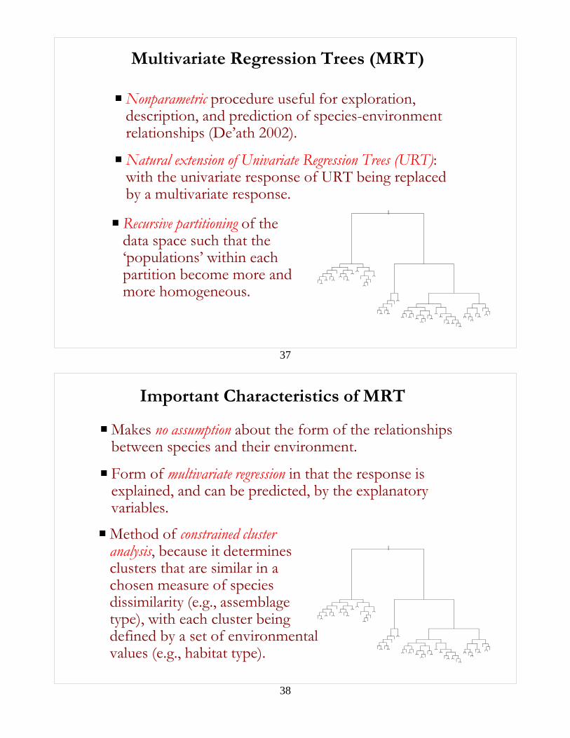
P Recursive partitioning of thedata space such that the‘populations’ within eachpartition become more andmore homogeneous.

38

P Makes no assumption about the form of the relationshipsbetween species and their environment.

P Form of multivariate regression in that the response isexplained, and can be predicted, by the explanatoryvariables.

Important Characteristics of MRT

P Method of constrained clusteranalysis, because it determinesclusters that are similar in achosen measure of speciesdissimilarity (e.g., assemblagetype), with each cluster beingdefined by a set of environmentalvalues (e.g., habitat type).

39

Univariate Regression Trees (URT)

1.At each node, the tree algorithm searches through thevariables one by one, beginning with x1 and continuing up toxM.

2.For each variable it finds the best split (minimizes the totalsums of squares or sums of absolute deviations about themedian).

3.Then it compares the M best single-variable splits and selectsthe best of the best.

4.Recursively partition each node until an over-large tree isgrown and then pruned back to the desired size (usuallybased on cross-validated predicted mean square error).

5.Describe each terminal node (mean, median,variance) andthe overall fit of the tree (% variance explained).

40


P Redefine node impurity by summing the univariateimpurity measure over the multivariate response.

< Minimize the sums of squared Euclidean distances(SSD) of sites about the node centroid.

P Additional ways to interpret the results of MRT:

< Identification of species that most stronglydetermine the splits.

< Tree biplots to represent group means and speciesand site information.

< Indentification of species that best characterize thegroups (ISA).

41


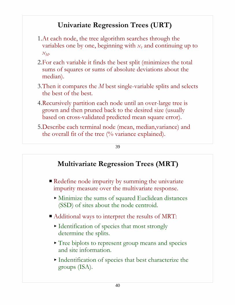
P Compare the MRT solution to unconstrainedclustering using a metric equivalent to the MRTimpurity and the same number of clusters.

P MRT can be extended to work directly from adissimilarity matrix; clusters can be formed bysplitting the data on environmental values thatminimize the intersite SSD.

|

42

MRT vs CCA vs RDA

P Unlike CCA/RDA, MRT is not a method of directgradient analysis, in the sense of locating sites alongecological gradients.

< MRT does locate sites (albeit grouped) in an ecologicalspace defined by the environmental variables.

P Unlike CCA/RDA, the MRT solution space is nonlinearand includes interactions between the environmentalvariables.

P MRT is a divisive partitioning technique; CCA/RDAmodel continuous structure.

0

0.5

1

1.5

2

2.5

3

3.5

1 10 19 28 37 46 55 64 73 82 91 100 109 118 127 136 145 154 163

43

MRT vs CCA vs RDA

P MRT emphasizes local structure and interactions betweenenvironmental effects; CCA/RDA determine globalstructure.

P MRT does not assume particular relationships betweenspecies abundances and environmental characteristics;CCA/RDA assume unimodal and linear response models.

|

44

MRT vs CCA vs RDA

P MRT has outperformed CCA/RDA in both simulated andreal ecological data sets in both explaining and predictingspecies composition.

P The advantage of MRT increases with the strength ofinteractions and the nonlinearity of relationships betweenspecies composition and the environmental variables.

|

Step 5: Conduct Analysis The CCA Algorithm

Documents

Transcript of Step 5: Conduct Analysis The CCA Algorithm