Stellar stability and asteroseismologydupret/Stab-et-astero-ang.pdfand the internal physical...
229
Stellar stability and asteroseismology SPAT0044 Marc-Antoine Dupret email: ma.dupret @ uliege.be web site : www.astro.ulg.ac.be/~dupret tel: 04 3669732 Bât. B5c, 1 er étage
Transcript of Stellar stability and asteroseismologydupret/Stab-et-astero-ang.pdfand the internal physical...

Stellar stability andasteroseismology
SPAT0044
Marc-Antoine Dupret
email: ma.dupret @ uliege.beweb site : www.astro.ulg.ac.be/~duprettel: 04 3669732Bât. B5c, 1er étage

Goals of the course
Precise mathematical problem
2) Understanding the underlying mathematical formalism
Asteroseismology
3) Understanding the link between stellar oscillations (frequencies, ...),and the internal physical structure of stars
Stellar stability
4) Understanding of the main energy processesat the origin of stellar oscillations
Pulsating stars in the HR diagram
5) Knowledge of the main families of pulsating stars, their theoretical characteristics and seismic probing potential
Stellar oscillations
1) Understanding the physics of stellar oscillations

Lecture notes and others
Powerpoint slides
Lecture notes « Stabilité Stellaire » of Richard Scuflaire
Lecture notes « Stellar Oscillations » of J.C. Dalsgaard
Methodology
Numerous analogies with other cases
- simpler (acoustic modes in an organ pipe, ...)
- well known (Schrödinger theory in quantum mecanics)

What are stellar oscillations ?

r(m) r’(m) = x r(m)
(m) ’(m) = (m)/x3
Poids(m) Weight’(m) = Weight(m)/x4
P(m) P’(m) = P(m) (’/)1 = P(m)/x3
1
First, hydrostatic equilibrium:
Homologous adiabatic contraction of the gas P’/P = (’/)1
If 1 < 4/3 Contraction (x < 1) P’(m) < W’(m) Force downwards
Force and displacement in the same direction
Collapse or explosion, dynamically unstable
If 1 > 4/3 Contraction (x < 1) P’(m) > Weight’(m) Force upwards
Expansion (x > 1) P’(m) < Weight’(m) Force downwards
Restoring force opposite to the displacement
Oscillations , dynamically stable
What are stellar oscillations ?Reminder : How a star reacts to a global contraction or expansion ?

What are stellar oscillations ?
In reality …
- The oscillation amplitude depends on the depth (not homologous)
- There are radial and non-radial oscillations
Amplitudes exagerated by a factor 106 !

- 2 possible restoring forces:
gradient of pressure Pressure modes
Archimedes force Gravity modes
What are stellar oscillations ?
In reality …
- The oscillation amplitude depends on the depth (not homologous)
- There are radial and non-radial oscillations

Characteristic times
Stellar oscillations = dynamical phenomenon
Characteristic time = dynamical time :
2
1
r
mG
dr
dP - −=
Dynamical time ~ free fall time
(pressure suppressed) GM
3
dyn
R t =22
dynt
R
R
GM=
Order of magnitude :
Other characteristic times:
(Forces imbalance)
Helmholtz – Kelvin time: Thermal imbalance
Nuclear time : Evolution due to nuclear reactions
Radial acceleration

Dynamical time : Forces imbalance
Always : tdyn << tHK << tnuc
At the time scale of oscillations :
1) The gas does not have time for significant heat exchange % heat capacity :
dq = T ds = du + P dv
|dq| << u ~ cv T In most of the star :
Oscillations are adiabatic
dq : Heat exchanged per unit mass during one oscillation cycle
Virial theorem :
Sun : 26 min 107 years 1010 years
Characteristic times
Helmholtz – Kelvin time: Thermal imbalance
Nuclear time : Evolution due to nuclear reactions

At the time scale of oscillations :
1) The gas does not have time for significant heat exchange % heat capacity :
2) The chemical composition does not have time to change :
In most of the star : oscillations are adiabatic
tdyn << tnuc
Period of oscillation (fundamental mode) ~ dynamical time
Dynamical times of some types of star :
Star
Neutron star
White dwarf
Sun
Red supergiant
1015 g/cm3
106 g/cm3
1.41 g/cm3
10-9 g/cm3
0.05 ms
2 s
26 min
2 ans
Characteristic times

Stars play music !

Solar type stars
A zoo of pulsating stars of different types
Thousands of observed modes !
Pressure modes(acoustic)
excited by turbulent motions at the top
of the convective envelope.
Periods ~ 3-8 min.
Helioseismology allows to probe:
- the sound speed, …
- the rotation speed
differential in the envelope.
Sun :

Pressure modes (acoustic).
Periods ~ 2-15 min.
Small amplitudes :
dL/L ~ 1-20 ppm, speeds ~ 1-20 cm/s
Modes difficult to detect,
Dozens of observed modes
Less information than in the
Solar interior.
Other stars (ex : ® Cen) :
A zoo of pulsating stars of different types
Solar type stars

Averaging over the disk

g Doradus
Gravity modes
Long periods ~ 0.5 - 3 days
Space revolution (Kepler, …):
Dozens of identified modes
Asteroseismology allows us to probe
their deep regions:
- Extension of the convective core,
“age”, core rotation, internal
composition, …
A zoo of pulsating stars of different types
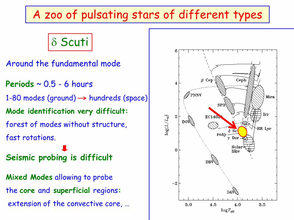
d Scuti
Around the fundamental mode
Periods ~ 0.5 - 6 hours
1-80 modes (ground) hundreds (space)
Mode identification very difficult:
forest of modes without structure,
fast rotations.
Seismic probing is difficult
Mixed Modes allowing to probe
the core and superficial regions:
extension of the convective core, …
A zoo of pulsating stars of different types

Rapidly oscillating Ap
High order pressure modes
Periods ~ 5.5 - 20 minutes
Strong magnetic field
Magneto-acoustic modes
Asteroseismology constrains
the internal magnetic field
Chemical peculiarities(diffusion process, …),Strong magnetic field
A zoo of pulsating stars of different types
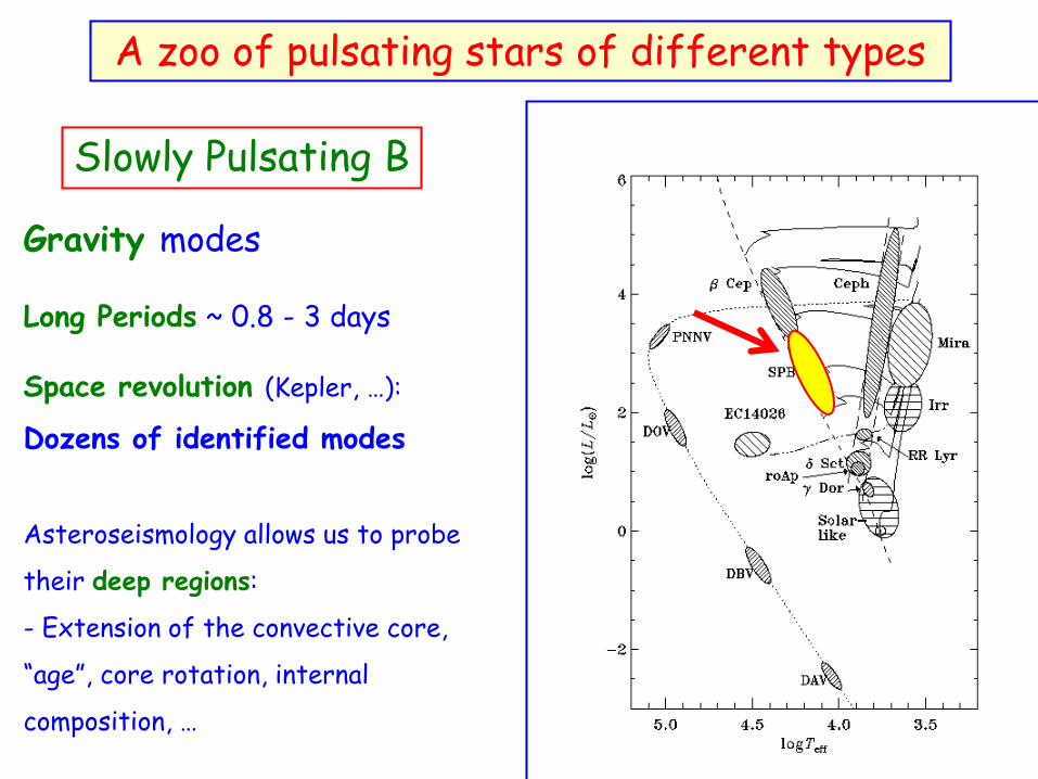
Slowly Pulsating B
Gravity modes
Long Periods ~ 0.8 - 3 days
A zoo of pulsating stars of different types
Space revolution (Kepler, …):
Dozens of identified modes
Asteroseismology allows us to probe
their deep regions:
- Extension of the convective core,
“age”, core rotation, internal
composition, …

Cephei
Around the fundamental mode
Periods ~ 2 - 8 hours
1-10 detected and identified modes
Successful asteroseismology
Mixed modes allowing us to probe:
- Deep regions :
extension of convective core,
internal rotation, …
- External regions : Opacities, chemical
composition, rotation, …
A zoo of pulsating stars of different types

Red giants
1) Radial mode(s) high amplitude :
Mira, irreg.
Periods ~ year(s)
2) Space revolution (Kepler, …):
Radial and non-radial modes (dozens) of
low amplitude excited by convection (~ sun)
Periods ~ 3-30 days
Asteroseismology : Detailed probing of the
superficial layers (p-modes) and the core
(thanks to mixed modes !)
Not enough for seismic probing
A zoo of pulsating stars of different types

High amplitude radial mode(s)
Periods :
RR Lyrae : 8 – 12 hours
Cepheids : 1 – 50 days
1 (or 2) modes
Classical instability strip :
Cepheids (d Cephei), RR Lyrae
Not enough for asteroseismology
Period – luminosity relation
Distance determination
A zoo of pulsating stars of different types

1) Near-fundamental modes
Periods : 1-10 minutes
2) Gravity modes (Betsy stars)
Periods : 0.5 - 3 hours
Stars having lost their envelope after the helium flash (binarity ?)
Asteroseismology :
Possibility of probing the interior of evolved
stars : internal chemical composition,
evolution channel of binary systems, …
Extreme horizontal branch(sub-dwarfs of type B, sdB)
A zoo of pulsating stars of different types

White dwarfs
Gravity modes
Different types :
- DOV (GW Vir) : Teff ~ 105 K,
Periods ~ 5 - 80 min.
- DBV (V777 Her) : Teff ~ 3 104 K
Periods ~ 2 – 15 min.
- DAV (ZZ Ceti) : Teff ~ 104 K
Periods ~ 0.5 – 25 min.
Asteroseismology :
Allows us to probe the interior of compact stars:
- Chemical composition of each layer,
- Equation of state (crystallization, degeneracy)
A zoo of pulsating stars of different types

Stellar hydrodynamics reminder
Lagrangian and Eulerian formalisms
2 types of spatial coordinates in fluid mechanics :
The 3 usual space coordinates (spherical coordinates r, µ, Á in stars)
1) Eulerian coordinates :
System of coordinates fixed in space, independent of motion
But not ideal to relate velocity and acceleration,
to follow changes of state and chemical composition
One notes /t the partial derivative % time in Eulerian coordinates.

2) Lagrangian coordinates :
System of coordinates (field of labels ) associated to each material
element of the fluid and following the motions.
Example, spherical symmetric star (1D) : mass of the spheres: m
The partial derivative % time in a Lagrangian coordinates system
is called the material derivative , one notes it : D/Dt
It is the variation % time following the fluid motions.
Coordinates change :
fixéTrajectories : Velocity :
General relation : Acceleration :
Stellar hydrodynamics reminder

Mass conservation :
Momentum conservation :
Poisson equation:
The Reynolds number associated with oscillations
is always very high the viscosity can be neglected
Stellar hydrodynamics reminder

Conservation of energy : (negligible viscous dissipation)
Transport of energy by radiation :
Transport of energy by convection :
Much more complicate !Rigorously, one should follow all the turbulent motions 3D simulations …
Stellar hydrodynamics reminder

Hydrodynamic simulations
Large Eddy Simulations (LES)
Main limitations :
Scales of 3D sim. >>> Dissipation scale
Age of stars >>> duration of 3D sim.
Real Reynolds nb. ~ 1010 >>> 104 in 3D sim.
Stellar convection
Analytical approaches: Mixing-length theory, …
Main difficulties in the description of convection :- Hydrodynamics involving a very large spectrum of space and time-scales :
~ 1cm (dissipation) up to the stellar size !
- Very very turbulent (Re ~ 1010 ) and non-linear
Very approximate
Introduction of free parameters …

Transport of energy by convection :
Much more complicate !Rigorously, one should follow all turbulent motions …
Analytical approach :
One separates : turbulent motions – average motion due to the oscillations
Turbulent motions lead to a new term in the energy equation,
the convective flux FC = cp Vc T (flux of enthalpy) :
Different approximate theories have been proposed relating the convective flux
to other quantities, for example the Mixing-Length Theory gives in the stationary
case without radiative loss :
But we don’t know how Fc reacts to oscillations…
Fc = cpT (P/)1/2
2(r - rad)
3/2
Stellar hydrodynamics reminder

Stellar convection and oscillations
Main difficult questions :
What are the transfers of energy between turbulent motions and oscillations ?
How the convective motions and the convective flux vary with time due to the oscillations ?
One must thus build models of time-dependent convection, which is much more complicate than getting stationary models .

Equilibrium (stationary) spherical symmetric configuration
24 rdr
dm=
Conservationof mass
2r
mG
dr
dP −=
Hydrostatic equilibrium
3216
3
Trac
L
dr
dT
−=Radiation
P
T
r
Gm
dr
dT2ad-
=Convection
Transferof energy
)(4 2
gravnrdr
dL +=
Conservationof energy
One notes the equilibrium solutions:
P0(r) , T0(r) , 0(r) , L0(r), …
One cancels all derivatives % time and the velocity in hydrodynamic simulations.
Efficient convection
adiabatic stratification

Theory of small perturbations
We start from an equilibrium model:
Study of the oscillations around this equilibrium.
One assumes that the oscillation amplitudes are small % scale heights.
Consequently, one can linearize the problem.
Eulerian and Lagrangian perturbations
1) Eulerian perturbation of X : X’
P0(r) , T0(r) , ½0(r) , L0(r)
Difference between instantaneous and equilibrium value at a fixed point in space.
2) Lagrangian perturbation of X : dX
Difference between instantaneous and equilibrium value for a fixed material element.

1) Eulerian perturbation of X : X’
2) Lagrangian perturbation of X : dX
Relation between Lagrangian and Eulerian perturbations :
Displacement vector :
Field of average positions: Lagrangian coordinates
One assumes that the oscillation amplitudes are small
1st order Taylor development :
Theory of small perturbations

Useful relations :
Lagrange – Euler :
Gradients :
Time derivatives :
O(2)
Sums :
Theory of small perturbations

Products :
Functions :
Cas particulier :
Products of powers :
Theory of small perturbations
Useful relations :

Integration % time :
Conservation of mass :
Integrated form of the
continuity equation:
Adiabatic stellar oscillations
Lag. coord. cst., t0 = time when ½=½0

Method of small perturbations :
One takes the difference between the dynamical and equilibrium equation:
Conservation of momentum :
Equilibrium configuration :
Adiabatic stellar oscillations

Poisson equation
Adiabatic expansion of the gas :
At the time-scale of oscillations, the gas has no time for significant heat
exchange % its heat capacity :
In the main part of the star, oscillations are adiabatic.
Adiabatic relation between pressure and density variation :
Adiabatic stellar oscillations
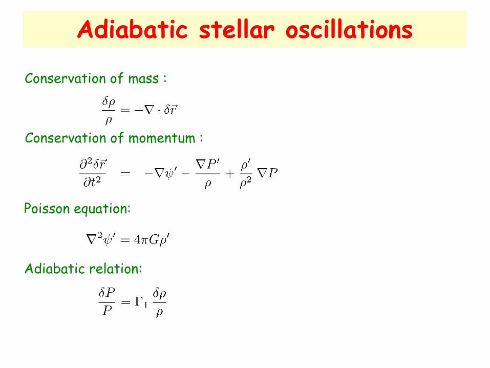
Conservation of momentum :
Conservation of mass :
Poisson equation:
Adiabatic relation:
Adiabatic stellar oscillations

Acoustic waves
Conservation of momentum :
Conservation of mass :
Adiabatic relation :
Homogeneous medium, no gravity :
Divergence of the momentum equation :
Wave equation : Sound speed c :

Wave equation : Sound speed c :
Stationary waves
Eigenvalue problem : A x = s2 x s2 : Eigenvalue
x = P’ : Eigenfunction (vector)
: Linear operator
+ boundary conditions
In a rectangular box [0, L1] x [0, L2 ] x [0, L3]
Rigid boundary conditions at the edges:
Solution :
Countable spectrumof frequencies
Eigenmode
The knowledge of the spectrum gives L1 /c, L2 /c and L3 /c
Frequency
Acoustic standing waves

1 dimension dP’/dr(0) = P’(R) = 0
R ,
T c ~ (P/)1/2 / T1/2 ,
c constant(T constant)
Rr
Large separation
Boundary conditions
n + 1 : nbre of nodes
0Frequency
P’
Acoustic standing waves in a semi-open organ pipe

R ,
T c ~ (P/)1/2 / T1/2 ,
In stars :
Radial modes Dynamical time
Rr
Large separation 0Frequency
Acoustic standing waves in a semi-open organ pipe
Rr
P’

C Non-constant
Temperature or section varying with r
What is the frequency spectrum ?
Particular case of a more general problem:
Sturm-Liouville problem
+ Homogeneous or periodic
boundary conditions:
p(x) > 0, (x) > 0 for a<x<b and continuous by part
In the organ pipe :
Acoustic standing waves in a semi-open organ pipe

Sturm-Liouville problem
Examples :
Organ pipe :
Legendre equation:
Bessel equation:
1D Schrödinger equation :
…
+ Homogeneous or periodic
boundary conditions:
p(x) > 0, (x) > 0 for a<x<b and continuous by part

Theorems :
1) Space
is a Hilbert space,
for the scalar product :
and u verifies theboundary conditions
2) Linear operator
is auto-adjoint (hermitian) :
Eigenvalue problem :
+ Homogeneous or periodic boundary conditions:
Sturm-Liouville problem

3) Orthogonality : The eigenspaces are orthogonal.
Let u and v be eigenfunctions of two different eigenspaces:
4) The eigenvalues li are real and form a countable series :
l0 < l1 < l2 < … < ln < …
5) The eigenfunctions ui form a complete orthogonal base:
1
Sturm-Liouville problem
Theorems :
+ Homogeneous or periodic boundary conditions:

5) The eigenfunction ui form a complete orthogonal base:
6) The nodes of the eigenfunctions are interlaced:
For i < j (li < lj), there is a node of uj between 2 nodes of ui.
7) Variational principle : The function (Rayleigh ratio)
is stationary
on the eigenspaces and is equal to the eigenvalues there.
Theorems :
+ Homogeneous or periodic boundary conditions:
Sturm-Liouville problem

Properties of the acoustic modes spectrum ?
This is a Sturm-Liouville problem
Corresponding properties:
Orthogonality,for 2 eigenmodes P’1 (r) and P’2 (r) :
Countable set of frequencies : 0 < s0 < s1 < … < sn < …
…Completeness : The eigenmodes form a complete base.
…Variational principle : Rayleigh ratio
is stationary on the eigenspaces.
Acoustic standing waves in a semi-open organ pipe
1

Radial adiabatic stellar oscillations
Conservation of momentum:
Conservation of mass:
Adiabatic relation:
Maintaining the spherical symmetry :
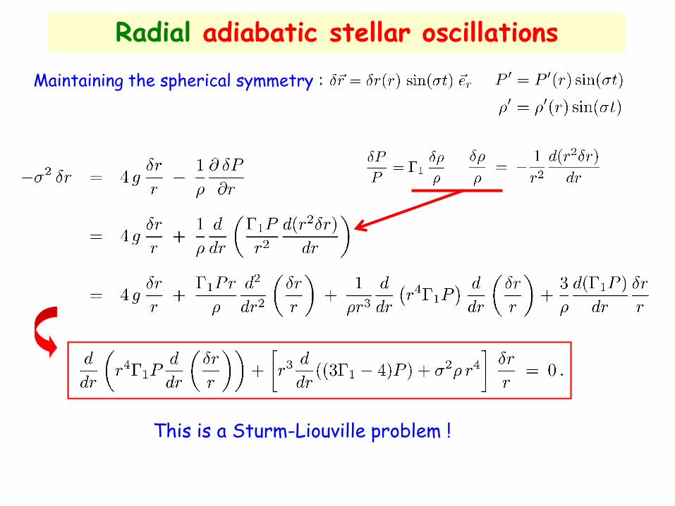
This is a Sturm-Liouville problem !
Maintaining the spherical symmetry :
Radial adiabatic stellar oscillations

Singular Sturm-Liouville problem (p(0) = p(R) = 0 )
Boundary conditions : Bounded solutions
bounded and regular at the center
0
At the center:
At the surface:
Radial adiabatic stellar oscillations

Sturm-Liouville problem
Corresponding properties:
- Orthogonality,for 2 eigenmodes x1 and x2 :
- Countable set of frequencies: s02 < s1
2 < … < sn2 < …
- Completeness: The eigenmodes form a complete base.
…- Variational principle:
is stationary on the eigenspaces and equal to si2 there.
Radial adiabatic stellar oscillations

Form of the eigenfunctions:
Fundamental mode
Polytrope n=3
1st overtone
Polytrope n=3
2nd overtone
Polytrope n=322th overtone
Sun
x = r/R
x = r/R
0.0 1.0
Not homologous !
Radial adiabatic stellar oscillations

General case :
Initial conditions :
General solution :
with
Proof :
complex
Linear combination of eigenmodes
Radial adiabatic stellar oscillations

with
Proof To show :
complex
Because is linear
Radial adiabatic stellar oscillations
General case :
Initial conditions :
General solution :

Dynamical stability of a star
The star is dynamically
stable
Sum of the oscillating solutions(standing waves) The star is dynamically
unstable
Unstable term
imaginary
2 possibilities :
sj real

r(m) r’(m) = x r(m)
(m) ’(m) = (m)/x3
Poids(m) Weight’(m) = Weight(m)/x4
P(m) P’(m) = P(m) (’/)1 = P(m)/x3
1
First, hydrostatic equilibrium:
Homologous adiabatic contraction of the gas P’/P = (’/)1
If 1 < 4/3 Contraction (x < 1) P’(m) < W’(m) Force downwards
Force and displacement in the same direction
Collapse or explosion, dynamically unstable
If 1 > 4/3 Contraction (x < 1) P’(m) > Weight’(m) Force upwards
Expansion (x > 1) P’(m) < Weight’(m) Force downwards
Restoring force opposite to the displacement
Oscillations , dynamically stable
What are stellar oscillations ?Reminder : How a star reacts to a global contraction or expansion ?

A star is dynamically unstable
Variational principle :
For a star to be dynamically unstable, we must have in a « significant » part of it:
in a significant part of the star
But one can have locally 1 < 4/3 and dynamical stability.
Question : What determines the behavior of 1?
Dynamical stability of a star
Rigorous definition :

slowly accretes matter from its red giant companion
1er scenario (most frequent): A white dwarf of C-O in a binary system
The C-O core reaches the Chandrasekhar’s limiting mass !
the C-O core grows in mass
2e scenario : During H and He shell burning,
Some case of dynamical instability …
1) C-O core reaching the Chandrasekhar’s limiting mass
The degenerated electrons reach relativistic speeds
e- capture by the nuclei : e- + p ! n + e
) e % ) P ¼ Pe (Ne) = Pe (/e) increases less ) 1 &
Dynamical stability of a star

The Nova phenomenon

Nuclear reactions in a degenerated medium thermal runaway
the entire star burns everything in a few seconds
The star explodes ! Type Ia supernova L ~ 109-10 L¯
- General relativity effects
Moreover:
The core collapses and reaches extreme densities
1) C-O core reaching the Chandrasekhar’s limiting mass
The degenerated electrons reach relativistic speeds
- e- capture by the nuclei : e- + p ! n + e
) e % ) P ¼ Pe (Ne) = Pe (/e) increases less ) 1 &
Dynamical stability of a star

Main scenario :
Core burning of Si, contraction,
Shell fusion of Si, contraction, …
) The Fe core contracts,
becomes degenerated and grows in mass.
When MFe ' Chandrasekhar’s mass
) collapse until the nuclei touch
each other ) rebound and chock wave
) Explosion, Type II Supernova
Onion-like structure
2) End of massive stars life
Dynamical stability of a star

Physical factors accelerating the collapse:
a) e- capture by the nuclei and free protons: e- + p ! n + e
) e % ) P ¼ Pe (Ne) = Pe (/e) increases less ) 1 &
b) Iron Photo-disintegration
T % ) Equilibrium towards the right : endothermic
) P, T increase less ) 1 &
c) Coulomb effects
% ) the electrons decrease the Coulomb repulsion between nuclei
) P increases less ) 1 &
2) End of massive stars life
Dynamical stability of a star

3) Hyper-massive stars ( )
The radiation pressure dominates
One shows that for ,
Very high temperature and low density
+ General relativity effects
The stars with are dynamically unstable
4) 2nd collapse of a proto-star
When Tc ~ 2000 K , dissociation : H2 H + H
Endothermic reaction 2nd collapse
Dynamical stability of a star

Asymptotic behavior of the frequencies
Question : Shape of the frequency pattern towards high overtones ?
Link with the internal structure ?
dP’/dr(0) = P’(R) = 0
c constant(T constant)
Large separation :
Boundary conditions
n + 1 : nbre of nodes
0Frequency
Acoustic waves in a semi-open organ pipe
Equidistant frequencies
Same asymptotic behavior in the general case ?

C Non-constant Temperature or section varying with r
Solution - approximation JWKB :
Proof :
0
General form :
One assumes
small
Asymptotic behavior of the frequenciesAcoustic waves in a semi-open organ pipe

JWKB approximation:
Boundary conditions
For large n, the frequencies are equidistant.
The knowledge of 0 or immediately gives :
This is the acoustic radius.
Asymptotic behavior of the frequencies
C Non-constant
Acoustic waves in a semi-open organ pipe

Non-radial adiabatic stellar oscillations
A stellar spectrum is often very rich, holding much more than radial modes only !
Some examples of non-radial oscillation modes …

Gradient :
One uses the usual spherical coordinates r, q, f
Hypothesis : The star oscillates around a spherically symmetric
equilibrium configuration
Small perturbations linear eigenmodes :
Useful reminder, differential operators in spherical coordinates:
Divergence :
Laplacian :
Non-radial adiabatic stellar oscillations

Conservation of momentum :
Conservation of mass :
Spherical symmetryand hydrostatic equilibrium
Non-radial adiabatic stellar oscillations

Legendrian :
Horizontal motion Conservation of mass
Conservation of masse+
Horizontal motion
Poisson equation :
Non-radial adiabatic stellar oscillations

System of partial derivative equations to solve :
Method of variable separation, one searches solutions of the form:
Possible here because the derivatives % q and f appear within the same operator
The spherical harmonics are eigenfunctions of
Solutions of the form:
Non-radial adiabatic stellar oscillations

System of 4th order ordinary differential equations in r to solve :
Solutions of the form:
We switched from a 3D (r, q, f) problem to a 1D (r) problem !
Non-radial adiabatic stellar oscillations

Spherical harmonics
m : Number of meridional node lines
l : Total number of node lines
l = 5
m = 2
l = 5
m = 0
Legendre associated function
Non-radial adiabatic stellar oscillations

One uses the adiabatic relation and eliminates ‘ to have 3
equations and 3 unknowns (xr, P’, ‘)
N : Brunt-Väisälä frequency Ll : Lamb Frequency
Radial motion
Horizontal motion + continuity
Poisson equation
Non-radial adiabatic stellar oscillations

One defines :
Displacement vector:
Continuity equation :
Non-radial adiabatic stellar oscillations

Without proof …
At the center : P’(r), Ã’(r), … / rl
l = 0 : »r / r l = 1 : »r(0) = »h(0) l > 1 : »r, »h / rl-1
At the surface : Perfect reflexion of the waves dP(R) = 0
Analytical solution of the Laplace equation
bounded at infinity :
Boundary conditions : bounded solutions at the edges
If ½(R) = 0 :
If ½(R) > 0 :
Non-radial adiabatic stellar oscillations

Cowling approximation:
Eigenvalue problem of 2nd order :
Justified when the number of nodes of ‘(r) is large
When the number of nodes of the eigenmodes is very large :
Oscillation cavities, pressure and gravity modesIntegral solution of the Poisson equation :
Non-radial adiabatic stellar oscillations

NB : a less approximate reasonning shows that,
Under the Cowling approximation, the equation to solve is:
with :
Non-radial adiabatic stellar oscillations
Oscillation cavities, pressure and gravity modes

If s2 > N2 and s2
> Ll2
ors2 < N2 and s
2< Ll
2
k2 > 0 wave equation
Wave propagation cavity
Local wave number : k
s2 > N2 and s2
> Ll2
Pressure mode-wave Gravity mode-wave
s2 < N2 and s2
< Ll2
Non-radial adiabatic stellar oscillations
Oscillation cavities, pressure and gravity modes

s2 > N2, Ll2
Pressure modes2 < N2, Ll
2
Gravity mode
k2 > 0 : Propagation cavity k2 < 0 : Evanescent zone
N2 < s2 < Ll2 or Ll
2 < s2 < N2s2 > N2 , Ll2 or s
2< N
2, Ll
2
Asymptotic solution (JWKB) : Asymptotic solution (JWKB) :
Non-radial adiabatic stellar oscillations
Oscillation cavities, pressure and gravity modes

Approximative JWKB solution :
Schroedinger equation :
Quantum physics : Schroedinger theory
V(r) < E Propagation zone of the particle
V(r) > E Evanescent zone
V(r) 0
de Broglie wavelength
Crossing of the barrier by quantum tunneling
Oscillation cavities, pressure and gravity modes

N / 2¼
The Sun :
p Cavity
L1 / 2¼
g Cavity
Radiative core Convective envelope
L5 / 2¼
L20 / 2¼
Oscillation cavities, pressure and gravity modes
Non-radial adiabatic stellar oscillations

Pressure modes
s12 < s2
2 < … 1
p1 p2 …
s12 > s2
2 > … 0
g1 g2 …
Limiting case : s2 >> N2, Ll2
Sturm-Liouville pb. :
Gravity modes Limiting case : s2 << N2, Ll2
Sturm-Liouville pb. : s1-2 < s2
-2 < … 1
Countable infinity of frequencies tending
towards infinity for each l
Oscillation cavities, pressure and gravity modes
Non-radial adiabatic stellar oscillations
Countable infinity of frequencies tending
towards zero for each l

Fundamental mode
For each l ¸ 2 , one find between the two countable infinities of g and p modes the fundamental mode, this is the only remaining mode in an incompressible sphere.
p1 p2 p3 …… g2 g1 f
Frequencies
0
Oscillation cavities, pressure and gravity modes
Non-radial adiabatic stellar oscillations
Pressure modes
s12 < s2
2 < … 1
p1 p2 …
s12 > s2
2 > … 0
g1 g2 …
Limiting case : s2 >> N2, Ll2
Sturm-Liouville pb. :
Gravity modes Limiting case : s2 << N2, Ll2
Sturm-Liouville pb. : s1-2 < s2
-2 < … 1
Countable infinity of frequencies tending
towards infinity for each l
Countable infinity of frequencies tending
towards zero for each l

Pressure (acoustic) modes
s2 >> N2, Ll2
Like for standing acoustic waves in an organ pipe :
The pressure modes in stars are comparable toacoustic standing waves.
An increase of the pressure resulting from the gas compression acts as a restoring force producing these waves.
The spectrum of oscillation frequencies of the pressure modes mainly depends on the sound speed profile c(r).
Asteroseismology (stars) or helioseismology (Sun) based onpressure modes enables to probe
Sound speed :

Asteroseismology (stars) or helioseismology (Sun) of pressure modesenables to probe the sound speed profile :
T Boundaries of
convective zones
Mean molecular weight
chemical composition :
helium abundance, …
Partial ionization zone,
equation of state, helium abundance
Pressure modes (acoustic)
In partial ionization zones, endothermic bound-free transitions :
During gas compression,part of the released
gravitational energy is pumped by the reaction
La pression augmente moins
¡1
Non-radial adiabatic stellar oscillations

Sun
Hundred thousands of pressure modes !!
l = 0 l ~ 200 !
Non-radial adiabatic stellar oscillations
Pressure modes (acoustic)

Non-radial adiabatic stellar oscillations
Pressure modes (acoustic)
Sun
Hundred thousands of pressure modes !!
l = 0 l ~ 200 !

s2 > N2, Ll2
N
L5L20
P Cavity
L1
Propagation cavity: s > Ll (r) Evanescent zone : s < Ll (r)
Non-radial adiabatic stellar oscillations
Pressure modes (acoustic)

Propagation cavity :
s > Ll (r)
Local representation (around ) of the mode as a plane standing wave:
Evanescent zone :
s < Ll (r)
Interpretation :
Pressure (acoustic) modes

Spherical harmonics
m : Number of meridional node lines
l : Total number of node lines
l = 5
m = 2
l = 5
m = 0
Legendre associated function
Non-radial adiabatic stellar oscillations

Propagation cavity:
s > Ll (r)
Point where s2 = Ll2 (r) :
N
L1L5
L20
Evanescent zone where:
s < Ll (r)
Sun
This is the turning point of the waves (rt)
The waves propagate with
the local sound speed
Non-radial adiabatic stellar oscillations
Pressure modes (acoustic)

Modes de pression (acoustiques)
N
L5L20L1
Different modes with different l, probe different layers of the star
Non-radial adiabatic stellar oscillations
p Cavity

s2 > N2, Ll2
DuvallRelation (1982)
JWKB approximation:
Boundary conditions :
At rt,
Pressure (acoustic) modes

s2 > N2, Ll2
Duvall relation (1982)
The resolution of the Duvall equation for different l and n
gives a good approximation of the Solar p modes frequency spectrum.
Theory ObservationsSun
n =
n =
n =
n =
Pressure (acoustic) modes

s2 > N2, Ll2
The Duvall relation shows very clearly the link between the
sound speed profile c(r) and the frequencies of p modes.
Knowing the observed frequency spectrum, one can probe the
sound speed profile through the inversion of this relation.
Pressure (acoustic) modes
The resolution of the Duvall equation for different l and n
gives a good approximation of the Solar p modes frequency spectrum.
Duvall relation (1982)

s2 > N2, Ll2
Very approximative asymptotic solution l << n :
Frequencyl = 0
l = 1
l = 2
Large separation ~ constant =
n
n
n
n+1
n+1
n+1
Pressure (acoustic) modes
Duvall relation (1982)

s2 > N2, Ll2
Small separation :
Very approximative asymptotic solution for l << n :
Large separationA better solution :
is large in the deep layers of a star,
the small separation informs us about these deep layers.
Pressure (acoustic) modes

Solar-type oscillations ( Centauri A)
Power spectrum of the star Cen A (Bouchy & Carrier 2002) :dozens of detected modes
The seismic study of these stars is much easier because :
- Regular structure of the spectrumeasy mode identification
- Slow rotationsimple modeling
l=
0
l=
2
l=
1
l=
0
l=
2
l=
1

Echelle diagram of 16 Cyg A observed by Kepler:54 detected modes
l=
0
l=
2
l=
1
l=
3
Frequency modulo large separation
Solar-type oscillations (16 Cyg)
The seismic study of these stars is much easier because :
- Regular structure of the spectrum
easy mode identification
- Slow rotationsimple modeling

As the star evolves, in the core
center surface
in the core
center surface
c2 c2
The small separation is an
indicator of the
evolution stage of a star.
dc/dr > 0
s2 > N2, Ll2
Small separation
is large in the deep layers of a star,
the small separation informs us about these deep layers.
Pressure (acoustic) modes

Seismic indicators :
Large separation :
Small separation :
Normalized small separation:
2nd order difference :
Independent of surface effects
Discontinuities of dc/dr :
Frontiers of convective
zones, …
s2 > N2, Ll2Pressure (acoustic) modes

The Sun
s2 > N2, Ll2
Thousands of modes
l = 0 l ~ 200 !
Seismic probing of the sound speed
Pressure (acoustic) modes

s2 < N2, Ll2Gravity modes
If s2 > N2 and s2
> Ll2
ors2 < N2 et s
2< Ll
2
kr2 > 0 Propagation cavity,
Local wave number : kr
s2 > N2 et s2
> Ll2
Pressure mode-wave Gravity mode-wave
s2 < N2 et s2
< Ll2
Reminder : Cowling approximation, |n|
s12 > s2
2 > … 0g1 g2 …

s2 << N2, Ll2
Physical interpretation of gravity modes
1)
2)
3)
>
~
During phase 2, the element has gone up
and is heavier than the surrounding medium :
Archimedes force downwards.
But the pressure gradient ensures equilibrium
along the radial axis :
the horizontal
pressure gradient pushes back the element
towards its initial state.
~
>
Gravity modes

s2 << N2, Ll2
1)
2)
3)
>
~
The Archimedes force
is the restoring force
The pressure gradient acts as a
force transmitter: although the
restoring force is radial,
the motions are mainly horizontal.
~
>
Gravity modes
Physical interpretation of gravity modes

N
L5L20
The Sun
p cavities
L1
g Cavity
Radiative core Convective envelope
s2 < N2, Ll2
Gravity modes have low frequencies,
they propagate in the deep layers (radiative core) of stars
Gravity modes

The spectrum of gravity mode frequencies depends on the Brunt-Vaïsälä frequency N(r)
Mean molecular weight gradient
Very precise probing of the
internal chemical composition
Super-adiabatic gradient
Probing of the temperature gradient
Derivatives Precise and localized constraints on the internal structure
s2 << N2, Ll2Gravity modes

Spectrum of ~ equidistant periods
1
The main quantity measured by asteroseismology
of g-modes is :
s2 << N2, Ll2
JWKB approximation :
Boundary conditions : : Cavity where s2 < N2, Ll2
Gravity modes

Brunt-Väisälä frequency for different types of stars
1) Main sequence (M > 1.5 M0)
N tdyn
X
N tdyn
r/R
m/M
m/M
Large values of N2 in the mean molecular-weight gradient region above the receding convective core.
N/r sg
Contracting core
g-modes frequencies enable us to measure the size of the convective core and probe the mean molecular-weight gradient region just above it.
d Scuti, 2.2 M¯
s2 << N2, Ll2
The g-modes frequencies increase as the star evolves (contrary to p-modes).
Gravity modes

2) Post-main sequence
Huge values of N
Very dense core
(N tdyn)2
Very dense frequency spectrum
of non-radial modes
Huge
B supergiant
s2 << N2, Ll2Gravity modes
Brunt-Väisälä frequency for different types of stars

Discontinuities of chemical composition :(H He, He C-O)
Peaks of N
Seismic probing of the envelope’s chemical composition
N towards the center :
g-modes probe the envelope !
Degenerated core : ~ P()
dlnP/dln ~ ln P/ln |s
3) White dwarfs
s2 << N2, Ll2Gravity modes
Brunt-Väisälä frequency for different types of stars

The internal chemical composition of a white dwarf revealed by asteroseismology !
Giammichele et al. 2018, Nature
s2 << N2, Ll2Gravity modes

p7
p6
p5
p4
p3
p2
p1
fg1
g2
g3 g4 g5 g6 g7 g8 g9 g10
As the star evolves :
R (Expansion of the envelope)
sp / (s0R dr/c)-1 / R-3/2
N/r (Contraction of the core)
sg / s N/r dr
The spectra of p- and g-modes cross : Avoided crossings
d Scuti
Mixed modes
Frequencies of p-modes:
Frequencies of g modes :
l = 2

s2 > N2, Ll2 in the envelope Pressure mode behavior
s2 < N2, Ll2 in the deep layers Gravity mode behavior
Cephei, d Scuti, evolved stars, …
N
g mode
p mode
L1
Mixed modes

p7
p6
p5
p4
p3
p2
p1
fg1
g2
g3 g4 g5 g6 g7 g8 g9 g10
Because of avoided crossings and the presence of mixed modes :
Desorganised spectrum
One observed some modes, who are they ?
Impossible to know based on the frequencies alone …
Need of mode identification
techniques based on other
observables
(line profile variations, …).
l = 2
Mixed modes

Fitting~100 peaks
Fitting~2000 peaks
X10
X10
A delta Scuti star observed by the CoRoT satellite:
More than hundreds of detected modes without regularity.
These stars have a high seismic potential but their study is very difficult :
- No structure of the spectrum(mixed modes)
difficult mode identification.
- Very fast rotationcomplex modeling.
Mixed modes

How red giants differ from the Sun ?
l = 0
l = 1
l = 2
Regular frequency pattern ~ Asymptotic
Small separation Large separation
Sun

Modes de pression (acoustiques)
N
L5L20L1
Non-radial adiabatic stellar oscillations
p Cavity

Acoustic structure of a red giantVery high density contrast between the core and the envelope
Mixed modes
Evolution core contraction N
Very high restoring force (Archimedes)
The mode behaves
here as a gravity mode
The mode behaves here
as a pressure mode
The two cavities are coupled through the evanescent zone
Mixed modes exhibiting the p- and g-like behaviors
The size of the evanescent zone increases with l

Huge number of
nodes in the core
Eigenfunctions similar
to classical p-modes in
the envelope
From Christensen-Dalsgaard (2004)
Acoustic structure of red giants and mode trapping

Mode trapping in red giants
Mode trapped in the core
Mode trapped in the envelope
Inertia of a mode
M=2 M¯, Log(L/L¯)=1.8, pre-He burning
Mixed modes

M=2 M¯, Log(L/L¯)=1.8, pre-He burning
Modes trapped
In the core
Modes trapped
in the envelope
Mode trapping in red giants
Mixed modes

Mixed modesMixed modes in a red giant

l=1 p-g avoided crossings
Observed
modes
From Bedding et al. (2011)
Mode trapping in red giants
Mixed modes

Mixed modes in red giants
- Stade évolutif
- Masse du cœur d’hélium
- Composition chimique interne
-1
He burning
H-shell burning

Variational principle
Reminder : oscillation equations :
Radial motion
Horizontal motion
Mass conservation
Adiabatic relation
Poisson equation
Non-radial adiabatic stellar oscillations

, and are linear functions of
is a linear operator
One defines the scalar product :
Variational principle
Non-radial adiabatic stellar oscillations

Scalar product :
The operator is self-adjoint :
One defines the function :
Variational principle :
The function is stationary
on the eigenspaces with S = si2
Variational principle
Non-radial adiabatic stellar oscillations

• The eigenvalues ¾i2 are real
• The eigenfunctions are orthogonal :
The variational principle will be very useful to establish the link
between the spectrum of oscillation frequencies { ¾i } and the internal
structure of stars : sound speed c(r), internal rotation (r), …
Variational principle
Non-radial adiabatic stellar oscillations
• The function is stationary
on the eigenspaces with S = si2

Question : Impact on the frequency spectrum { ¾i } ?
Consider a small modification of the internal equilibrium structure of a star :
c0(r) c0(r) + c(r)
0(r) 0(r) + (r)
0(r) 0(r) + (r) …
Let { ¾i0 , »i0 } be the frequencies and eigenfunctions of the initial model (c0(r), …)
and the operator such that
Modificaton of c(r), … The coefficients of the equations are modified
Modification of the frequencies :
Variational principle
Non-radial adiabatic stellar oscillations

Modification of the frequencies :
Demonstration :
Variational principle
Non-radial adiabatic stellar oscillations

Variational principle for te organ pipe
kernel
P0 constant, c02(r)
Inverse problem
Given measured frequencies : ¾i,obs
Given reference model with theoretical frequencies : ¾i,th
Question : Which change ¢c2(r) gives the agreement theory – observations
Answer : One has to solve the inverse problem :
Known Unknown function
Known

JWKB approximation:
Boundary conditions
For large n, the frequencies are equidistant.
The knowledge of 0 or immediately gives :
This is the acoustic radius.
Asymptotic behavior of the frequencies
C Non-constant
Acoustic waves in a semi-open organ pipe

Inverse problems
General formulation :
For given functions b(x) and K(x,y), find f(y) such that
Examples :
Kernel
Deconvolution :
Earth seismology :
ds
r0
R(µ)
One mesures the arrival times of seismic waves
at different points of the globe .
One deduces the internal P and S waves speed
profiles by solving the inverse problem :
µ
For given functions b(x) and g(x), find f(y) such that

Inverse problem: non-radial stellar oscillations
p modes sound speed profile and internal chemical composition
Given measured frequencies : ¾n,l,obs
Given reference model with theoretical frequencies : ¾n,l,th
Inverse problem :
Given Sound speed and density profiles to determine
Equation of state : c2 = c2(½, P, Y, Z)
One can probe the internal composition profile and thus constrain the macroscopic
(rotation, …) and microscopic (diffusion, …) transport processes of chemicals.
small
From the equation of hydrostatic equilibrium, ¢P/P can be determined :

Helioseismology
Examples of kernels (l=0, n=21)¢c2/c2 and ¢½/½ obtained by seismic
inversion inversion from solar p-modes
Inverse problem: non-radial stellar oscillations

Signatures of sharp variations: the organ pipe
Effect of a local change of the sound speed:
JWKB approximation:
Seismic signature of the local change : oscillating component in
~
n
Dirac

Signatures of sharp variations: g-modes (SPB, g Dor)
Sharp variation of N at r
Periodicity of P(k) :
Variational principle :
Amplitude of the discontinuity
Localisation of the transition
Indicator of Xc and thusthe evolution stage
m(r)
m(r0)

Constraints on extra-mixing due to rotation, g-modes (SPB, g Dor)
The turbulence induced by
differential rotation smoothens the
X profile above the convective core
Hence, it smoothens the Brunt-
Vaïsälä frequency profile

The turbulence induced
by differential rotation
decreases the amplitude
of the periodic signal in
P(k)
Constraints on extra-mixing due to rotation, g-modes (SPB, g Dor)
The turbulence induced
by differential rotation
smoothens the X profile
above the convective
core

Direct method in asteroseismology
For most stars, except the Sun, not enough detected and identified frequencies for using seismic inversion techniques.
Direct seismic methodObservational data :
- Observed frequencies : {ºobs,i}.- Non-seismic constraints, ex : L/L¯, Teff , log g (color indices,
spectroscopy), surface chemical composition (spectroscopy), R (interferometry), M (binarity), … with error bars !
Goal :To find a stellar model matching as well as possible the seismic and non-seismic measurements.
Method :
One reduces the solution space by assuming that the stellar structure models only depend on a finite number of free parameters {ai} such as : the stellar mass, age, initial mass fractions of hydrogen (X) and heavy elements (Z), mixing-length (®) and overshooting (®ov) parameters, …One determines the values of these parameters providing a model matching as well as possible the observations through the minimization of a merit function.

Set of free parameters
a1, a2, …, aM
Minimization of :
Theoretical frequencies Observed frequencies
Méthode :One reduces the solution space by assuming that the stellar structure
models only depend on a finite number of free parameters {ai} such as : the stellar mass, age, initial mass fractions of hydrogen (X) and heavy elements (Z),
mixing-length (®) and overshooting (®ov) parameters, …One determines the values of these parameters providing a model
matching as well as possible the observations through the minimization of a merit function.
Computation of the
corresponding structure model
Computation of the oscillation
frequencies by solving:
2 evaluation and choice of a new set of free parameters
Iteration
Direct method in asteroseismology

Rotation Reminder, oscillation equations without rotation :
- Spherical symmetry: the equilibrium quantities only depend on r .
- The only angular differential operator appearing in these equations is :
-
Partial derivative equations Variable separation (spherical harmonics)ordinary differential equations
Variable separation because :
Non-radial adiabatic stellar oscillations

Rotation
Analogy with quantum physics :
Bohr model of the hydrogen atom – Non-radial oscillations without rotation :
For a fixed l, the energy levels (resp. the oscillation frequencies) are identical for
the 2l+1 possible values of m (-l · m · l).
Without rotation, the equations and thus the solutions (frequencies, …) do
not depend on the azimutal order m. For a fixed l , they are the same for
the 2l+1 possible values of m (-l · m · l).
This degenerecy of the solutions comes from the spherical symmetry.
Non-radial adiabatic stellar oscillations
- Spherical symmetry: the equilibrium quantities only depend on r .
- The only angular differential operator appearing in these equations is :
-
Variable separation because :
Reminder, oscillation equations without rotation :

Rotation breaks the spherical symmetry
It lifts the m degeneracy
Rotation modifies the equations of the problem.
In a corotating frame, 2 additional (fictious) forces
appear in the equation of momentum conservation :
the centrifugal force and the Coriolis force.
Non-radial adiabatic stellar oscillations
Rotation

1) The « Doppler effect » due to rotation
Rigid rotation models (Oscillations around the) corotating frame.
Approximation : One neglects the centrifugal and Coriolis forces
Same equations as before from the point of view of the corotating frame.
Inertial frame: Corotating frame :
Spherical coord. (r, µ, Á) Spherical coord. (r’, µ’, Á’) = (r, µ, Á - t)
Angular rotation speed
Same equations in the corotating frame
same solutions :¾0 : frequency
without rotationIn the inertial coordinates system :
From the observer’s point of view, the measured frequency is:
Non-radial adiabatic stellar oscillations
Rotation

1) The « Doppler effect » due to rotation
From the observer’s point of view, the measured frequency is :
Rotational splitting
triplet quintupletl = 1 l = 2
…Frequencies :
m = 1 0 -1 2 1 0 -1 -2
The rotational « splittings » give a
measure of the rotation
Non-radial adiabatic stellar oscillations
Rotation

1st order perturbative treatmentRotation :
Centrifugal force neglected spherical symmetry
Corotating frame where the frequency is ¾c
Coriolis acceleration taken into account:
Equation of motion (in the corotating frame) :
Without rotation With rotation (corotating frame)
Effect of rotation treated as a small perturbation of the problem to solve :
The variational principle can be used to determine the
effect of rotation (Coriolis) on the frequencies.
Non-radial adiabatic stellar oscillations

In the corotating frame (acceptable if rotation is rigid) :
1st order perturbative treatmentRotation :
Non-radial adiabatic stellar oscillations
Without rotation With rotation (corotating frame)
Effect of rotation treated as a small perturbation of the problem to solve :
The variational principle can be used to determine the
effect of rotation (Coriolis) on the frequencies.

1st order perturbative treatmentRotation :
Non-radial adiabatic stellar oscillations

1st order perturbative treatmentRotation :
Non-radial adiabatic stellar oscillations

From the point of view of the observer, the measured frequency is :
Ledoux constant
p modes :
g modes :
Differential rotation (r)
From the point of view of the observer :
1st order perturbative treatmentRotation :
Non-radial adiabatic stellar oscillations

In the corotating frame (acceptable if rotation is rigid) :
In the inertial frame, (r) :
1st order perturbative treatmentRotation :
Non-radial adiabatic stellar oscillations

triplet quintupletl = 1 l = 2
…Frequencies :
m = 1 0 -1 2 1 0 -1 -2
Inverse problem
Rotational multiplets : ¢¾i
One searches (r) such that
1st order perturbative treatmentRotation :
Non-radial adiabatic stellar oscillations

Sun, general case (r, µ)
Internal rotation profile in the Sun obtained by helioseismic inversion
• Differential rotation
in the envelope
• Rigid rotation in the
radiative core
Due to the transport of
angular momentum by
gravity waves
(Charbonnel & Talon 2005)
Inversion of rotation

Probing internal rotation :Kernels
HD 129929
Eridani
Cephei
2 observed multiplets but they probe
rotation in different layers because
their kernels are very different.
core ~ 3 surf
However, in other stars (ex: µ Oph),
rigid rotation cannot be rejected.
Action of the magnetic field ?
The determination of (r) provides contraints on angular
momentum transport processes.
Result here :

Effects of fast rotation
1. If rot2 << GM/R3
The star is significantly flattened by the centrifugal force
2. If rot << s
Significant impact of the Coriolis force on the
oscillations dynamics Gravito-Inertial modes
- The rotational multiplets are no
longer equidistant. 1st order
2nd order
- The dependence in µ, Á of the
eigenfunctions is no longer given
by spherical harmonics.
Effect of fast rotation on a multiplet

The traditional approximation (gravito-inertial modes)
One neglects the centrifugal force spherical symmetry
We take the corotating frame as reference where the (ang.) frequency is ¾c
We take the Coriolis acceleration into account:
Equation of motion (in the corotating frame) :
We consider gravito-inertial modes for which << sc
The perturbative approach is not justified for the modeling of
the effect of rotation on frequencies.
Non-perturbative approach required
Effects of fast rotation

Eq. of motion :
One considers gravito-inertial modes for which
radial displacements << horizontal displacements
- One neglects the radial component of the Coriolis force
- One neglects the radial displacement in the horizontal
component of the Coriolis force one neglects q
- One neglects ‘ (Cowling approximation)
The traditional approximation (gravito-inertial modes)
Effects of fast rotation

One isolates xq and xf :
Substitutes them in the continuity equations:
The traditional approximation (gravito-inertial modes)
Effects of fast rotation

The traditional approximation (gravito-inertial modes)
Effects of fast rotation

Laplace tidal equation
Method of variables separation, one searches solutions of the form :
Solutions : Hough functions
The traditional approximation (gravito-inertial modes)
Effects of fast rotation

Differential equations of the problem :
This is the nearly the same problem as before, l(l+1) has been replaced by l !
Same properties of the solutions for gravito-inertial modes :
Propagation cavity :
Local wave number :
Asymptotic periods :
Butis a function of and thus of the frequency as well as m
The traditional approximation (gravito-inertial modes)
Effects of fast rotation

Why stars are pulsating ?
Why some modes are observed and others are not ?
What determines the amplitudes and phases of oscillations ?
What determines the growth or damping rates of oscillations ?
Can we get additional constraints from other observables
than the frequencies ?
Non-adiabatic asteroseismology enables to address these questions.
Energetical aspects of stellar oscillations
Questions :

Reminder, characteristic times
Helmholtz – Kelvin time-scale : Thermal desequilibrium
Nuclear time-scale : Evolution due to nuclear reactions
Dynamical time-scale : Forces desequilibrium
One has always : tdyn << tHK << tnuc
Global reasoning: At the time-scale of oscillations, the gas has no time
to exchange significant heat compared to the global heat capacity of the star.
dq = T ds = du + P dv
|dQ| << u M ~ cv T M In the main part of the star :
oscillations are adiabatic
Q : Heat exchanged during one oscillation cycle
Virial theorem:
Sun : 26 min 107 ans 1010 ans

dq = T ds = du + P dv
|Q| << u M ~ cv T M
Local reasoning: Same reasoning but for the superficial layers only.
We have seen that globally :
But in near-surface layers, the heat exchanged per unit mass is of the same order as
the internal energy:
The heat capacity of the superficial layers is of the same order (or smaller)
than the heat exchanged during one oscillation cycle.
Oscillations are thus non-adiabatic there.
Global reasoning: At the time-scale of oscillations, the gas has no time
to exchange significant heat compared to the global heat capacity of the star.
Reminder, characteristic times
Q : Heat exchanged during one oscillation cycle
Virial theorem:
In the main part of the star :
oscillations are adiabatic

log tth: Thermal relaxation time
Quasi-adiabatic region :
¿th >> Period
In the main part of the star in term of mass,
oscillations are adiabatic.
The frequencies are accurately computed in
the frame of the adiabatic approximation.
Non-adiabatic
region :
¿th < Period
ds/cp 0
We will see that the main excitation
of the oscillation modes occurs in
the transition zone where the
thermal relaxation time and the
periods are of the same order.
I define the thermal relaxation time as :
In the superficial layers, the
oscillations are non –adiabatic :
To model oscillations there, one has
to solve the coupled
- Dynamical equations :
Conservation of momentum
and mass, Poisson equation.
- Thermal equations :
Conservation and transport
of energy.
Reminder, characteristic times

Radial non-adiabatic oscillations
Equations of the problem
Oscillations around a model in thermal equilibrium :
Conservation of momentum :
Conservation of mass :
:
Conservation of energy :

Equations of the problem
:
Unknowns :
Transfer of energy (radiative zone) :
Equations of state :
Nb. of equations : 4
Radial non-adiabatic oscillations

Equations of the problem
The characteristic times associated to each intermediate reaction are very different.
Nuclear reactions :
g+→+ HeHH 3
2
2
1
1
1
HHeHeHe 1
1
4
2
3
2
3
2 2+→+
Examples : - Deuterium burning :
- He3 burning :
Very short reaction time tD ~ 1 sec << Oscillation period
Out of equilibrium, ¿He3 >> Périod of oscillation
During the oscillations, the reactions are out of equilibrium.
The variation of the abundances of nuclei depends on the oscillation period.
One cannot simply perturb the equilibrium equation :
The perturbation of ² depends on the frequency :
Radial non-adiabatic oscillations

Solutions in the complex plane
i in the energy equation :
The solutions of the problem are complex :
¾ and dX(r) are complex
For classical pulsators, one expects that the observed modes are vibrationally unstable
Mean to confront theory and observations !
h is the mode’s growth rate:
− h > O The mode is vibrationally unstable.
− h < 0 The mode is vibrationally stable.
The vibrational instability is a form of thermal instability dynamical instability.
Associated time-scale = Helmholtz-Kelvin time-scale (GM2/(RL)) >> dynamical time.
h / sR ~ tdyn / tHK << 1
Radial non-adiabatic oscillations

¾ and dX(r) are complex
f(r) is the phase of the considered quantity.
It varies as a function of depth and from a quantity to another
Phase shifts between the different quantities.
Examples :
- Phase-shift between the light curve (photometric variability) and
velocity curve (Spectroscopic Doppler effect).
- Phase-shifts between photometric variations in different passbands
(Photometric multi-color filters of Johnson, Strömgren, …)
Other means to confront theory and observations !
Radial non-adiabatic oscillations
Solutions in the complex plane :

Work and energy
Energy of a mode :
Adiabatic oscillations :
Kinetic energy (/ u. vol.) :
Adiabatic oscillations are conservative
The energy of the mode is conserved in each layer.
Potential energy (/ u. vol.) :
Total energy (/ u. vol.) :
Global mode Energy (integrated over the full volume) :
Radial non-adiabatic oscillations

Work performed during one oscillation cycle (/ u. mass) :Non-adiabatic
oscillationsphase-shifts
Global work performed during one oscillation cycle :
Mean power :
Radial non-adiabatic oscillations
Work and energy

The work integral :
Equation of motion and integration :
Imaginary part of the result :
Radial non-adiabatic oscillations
Work and energy

This result is easily understood :
With (the mean power = the increase of energy / u. time),
one recover the work integral.
Radial non-adiabatic oscillations
Work and energy
The work integral :

The work integral, thermal analysis
The vibrational stability is associated to the non-adiabatic character of oscillations.
Radial non-adiabatic oscillations
Work and energy

Thermodynamical cycle
Condition for vibrational instability: during the hot phase of pulsation :
the gas must receive heat from the surrounding : .
This is a well-known property of thermodynamical cycles :
Condition for a motor thermodynamical cycle :
Heat must be received by the system at the hot phase and
provided outside at the cold phase.
Classical example : the Carnot cycle.
Radial non-adiabatic oscillations
Work and energy

Heat out at the Cold phase
Heat in at the Hot phasePositive work
Work = s P dV= Area
Carnot cycle
Isothermal :
PV = cst.
dQ = p dV
Adiabatic :
PVg
= cst.
-cv dT = p dV

The - mechanism
We focus now on the envelope where = 0 and examine the
conditions for at the hot phase.
For the - mechanism, the opacity variations produce the
« heat trapping » at the hot phase.
Term at the origin of the - mechanism
Radial non-adiabatic oscillations
Condition for vibrational instability: during the hot phase of pulsation :
the gas must receive heat from the surrounding : .

Modes’ driving : The - mechanism
log T
κ
SurfaceCenter
Opacity peak due to a partial ionization zone :
He+ He++ (log T ~ 4.5, Cepheids, RR Lyrae, d Scuti)
Fe, level M (log T ~ 5.2, Cephei, SPB, sdB)
The opacity mainly depends on the temperature

T
κ
Hot phase
Surface
Hot phase : heat enters but cannot go out.
Modes’ driving : The - mechanism
The opacity mainly depends on the temperature
Center
Opacity peak due to a partial ionization zone :
He+ He++ (log T ~ 4.5, Cepheids, RR Lyrae, d Scuti)
Fe, level M (log T ~ 5.2, Cephei, SPB, sdB)

κ
Surface
Cold phase : heat cannot enter but goes out easily.
T
Cold phase
Modes’ driving : The - mechanism
Center
The opacity mainly depends on the temperature
Opacity bump due to a partial ionization zone :
He+ He++ (log T ~ 4.5, Cepheids, RR Lyrae, d Scuti)
Fe, level M (log T ~ 5.2, Cephei, SPB, sdB)

• Around the opacity bump:
Positive work excitation of the mode (input of mechanical energy)
Region having the largest weight (excitation or damping) :
Transition region where Thermal relaxation time ~ Pulsation period
• Out of the opacity bump :
Negative work damping of the mode (loss of mechanical energy)
Final result : Vibrational stability (damping of the mode)
or instability (excitation of the mode)
depending on the weight of the opacity bump region .
Modes’ driving : The - mechanism
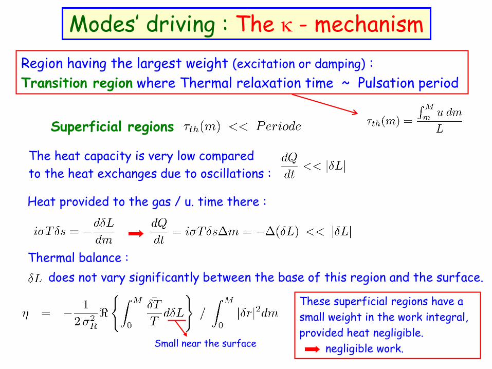
The heat capacity is very low compared
to the heat exchanges due to oscillations :
Superficial regions
Heat provided to the gas / u. time there :
does not vary significantly between the base of this region and the surface.
These superficial regions have a
small weight in the work integral,
provided heat negligible.
negligible work. Small near the surface
Thermal balance :
Modes’ driving : The - mechanism
Region having the largest weight (excitation or damping) :
Transition region where Thermal relaxation time ~ Pulsation period

Deep regions
Large in the deep regions.
The deep layers have a small weight
in the work integral because the
variations of the heat flux due to
oscillations are small there. Small in the deep layers
The amplitude of the eigenfunctions is much smaller there than near the surface.
Ex : approx. JWKB :
In particular, and are very small there small heat exchanges,
quasi-adiabatic oscillations negligible work.
Modes’ driving : The - mechanism
Region having the largest weight (excitation or damping) :
Transition region where Thermal relaxation time ~ Pulsation period

For efficient excitation (driving) of the oscillations, the
opacity bump must be located in the transition region.
Modes’ driving : The - mechanism
• Around the opacity bump:
Positive work excitation of the mode (input of mechanical energy)
• Out of the opacity bump :
Negative work damping of the mode (loss of mechanical energy)
Region having the largest weight (excitation or damping) :
Transition region where Thermal relaxation time ~ Pulsation period
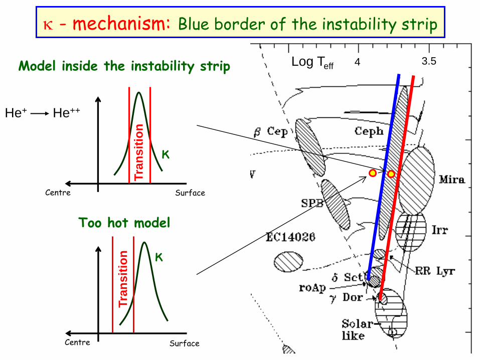
- mechanism: Blue border of the instability strip
Too hot model
κ
Centre
Tra
nsit
ion
Surface
κ
SurfaceCentre
Tra
nsit
ion
Model inside the instability strip Log Teff 4 3.5
He+ He++

Log Teff 4 3.5
In a Cephei,The Fe opacity bump is near
the surface it coincides
with the transition zone of
(low n) p-modes .
Frequency transition zone closer to the surface
g50
Log t
em
ps therm
ique
(Fe bump, layer M)
- mechanism : Pressure and gravity modes
Example : Cephei (pressure) – SPB (gravity)

Log Teff 4 3.5
g50
Log t
em
ps therm
ique
In a SPB, the Fe opacity bump
is deeper It coincides with
the transition zone of high-order
gravity modes.
Frequency transition zone closer to the surface
(Fe bump, layer M)
Example : Cephei (pressure) – SPB (gravity)
- mechanism : Pressure and gravity modes

Log Teff 4 3.5
Other similar example :
Subdwarfs of B type (sdB) :
Stars having lost their whole envelope
after the helium flash
below the main sequence.
g50
Log t
em
ps therm
ique
Fer opacity bump coincides also with thetransition zone
Pressure modes
Gravity modes
- mechanism : Pressure and gravity modes
Frequency transition zone closer to the surface

Modes’ excitation strongly depends on the height (and shape) of the opacity bump
The range of observed excited modes enables us to constrain the opacity.
How well do we know opacities ?
1. Uncertainties in opacity computations :
Huge number of transitions (bound-bound, bound-free), inaccuracies in cross-
sections computations (orbit-orbit, spin-orbit,spin-spin couplings, …).
Ex: Before 1990, impossible to explain the driving of Cephei pulsations because
the opacities due to Fe transitions were underestimated (neglected transitions).
Differences between opacity tables remain, inaccuracies are still present.
Non-adiabatic asteroseismology
Contraints on the micro-physics : matter-radiation interaction
- mechanism : non-adiabatic asteroseismology

2. Chemical composition : Abundance of absorbing ions
Ex: Cephei, SPB, sdB : Main contributors to the opacity at T~ 2£ 105 K :
Fe group elements (transitions from the M-layer): Fe, Ni, …
Constraints on chemical transport processes :
Radiative forces, gravitational settling, transport by gravity waves,
turbulence and meridional circulation due to differential rotation, …
Local accumulation of Fer, Ni, … Increases the opacity bump
The driving of the numerous observed modes in many sdB, Cep (in the LMC
& SMC, Z = 0.0025), … is not explained yet !
Modes’ excitation strongly depends on the height (and shape) of the opacity bump
The range of observed excited modes enables us to constrain the opacity.
How well do we know opacities ?
- mechanism : non-adiabatic asteroseismology

But … With a homogeneous chemical composition
= the observed surface one,
impossible to explain
the modes’ driving.Charpinet et al. 2001
– mechanism in the
Fe partial ionization zone
- mechanism, ex : Subdwarfs B (sdB)
damping
driving

Dynamical equilibrium
gravitation = radiative forces
Fe
Fe
Fe
Charpinet et al. 2001
Fe
Diffusive time¿
Evolution time
Consequence: local
accumulation of Fe
at T ~ 2 £ 105 K.
Opacity bump and thus
–mechanism reinforced
More excitation
- mechanism, ex : Subdwarfs B (sdB)

Very short wavelength oscillations
Large variations of the T gradient with heat loss at the hot phase and heat gain at the cold phase.
Strong radiative damping
Huge N2
huge
Non-radial modes are strongly damped in the core and cannot be observed
Except modes trapped in the envelope
In post-main sequence evolved stars:
Huge density constrast between the very dense
core and the very diluted envelope
Radiative damping mechanism
l = 1, f = 14.4 c/d ~ mode fondamental radial
xh
xr

2) Post-main sequence
Huge values of N
Very dense core
(N tdyn)2
Very dense frequency spectrum
of non-radial modes
Huge
B supergiant
s2 << N2, Ll2Gravity modes
Brunt-Väisälä frequency for different types of stars

dT> 0
dT<0
Very short wavelength oscillations
Large variations of the T gradient with heat loss at the hot phase and heat gain at the cold phase.
Strong radiative damping
huge
Non-radial modes are strongly damped in the core and cannot be observed
In post-main sequence evolved stars:
Huge density constrast between the very dense
core and the very diluted envelope
Except modes trapped in the envelope
Radiative damping mechanism
Huge N2

1. In g Dor stars, around the red border of the instability strip,
in solar-type stars, red giants, white dwarfs :
Transition zone inside the convective envelope.
Convection plays a key role in the modes’ excitation and damping.
In all cases (except part of g Dor stars) :
Convective time-scales < ~ pulsation periods
2.
Important coupling between convection and oscillations
No good theory…
Comparaison with observations :
Frequency interval of excited modes,
Instability strips (red border) …
Contraints on convection
and its time-dependent
interaction with oscillations
Convection : effect on the modes’ excitation and damping

A simple case: Convective blocking
g Doradus
The transition regioncoincides with the base of the convective envelope.
The heat exchanges in this region are at the origin of the g-modes’ driving.
Radiative zone Convective envelope
At the hot pase of the oscillations, rT more heat enters in the
convective envelope.
Heat
Convection does not adapt instantaneously to the oscillations.
Heat flux is blocked
The heat provided to the base of the convective envelope is converted into mechanical energy of the g-modes.
Excitation
Type F, main sequence, g-modes

Instability regionsFor efficient driving, the transition region must coincide with the base of the convective envelope.
l = 1
The size of the convective envelope is not know accurately.
It can be constrained by comparing the theoretical and observed instability regions.
Mixing length parameter = 1, 1.5, 2
Teff Convective envelope’s size
Convective envelope’s size Instability region moves
to the red (Teff )
A simple case: Convective blocking
g Doradus Type F, main sequence, g-modes

Another “simple” case: White dwarfs
Teff = 19830 K
Teff = 26790 K
Teff = 22040 K
tconv (s)
Convective time-scales (~ 1 s)
Convection adapts quasi-instantaneously to the oscillations
Models of time-dependent convection
are simpler.
However, the red borders of
instability strips are still unexplained.
Convective time-scales
Periods of pulsation
Pulsation periods (g-modes, P ~ 500 s)<<

Stochastic excitation : Solar-like oscillations
Oscillations are damped (coherent interaction with convection)
h : damping rate, 1/h : mode’s lifetime
The Sun seen as a drum
M 2
2
h
PVs =
Turbulent convective motions at the top of the convective envelope
hit the drum (stochastic forcing).
P : power injected in the acoustic modes by turbulence
Power injected by turbulence
Damping rateMode « Mass » :
M
Mean quadratic speed of the mode

The problem of mode identificationIn all pulsating stars except solar-like stare :
mode identification (l, m, n ??) is difficult …
Phase-lags
Line-profile variations Amplitude ratios
Very sensitive to the non-adiabatic
modeling of time-dependent convection
Spectroscopy Photometry
Additional observables for mode identification

Monochromatic magnitude variationsdue to non-radial oscillations
• The distorsion of the stellar surface corresponds to the material
displacement at the photosphere
• Local variations of the
mono-chromatic flux:
• Limb darkening :
• Thermal equilibrium in the atmosphere
Hypotheses :
To integrate over the entire visible disk
• Non-radial modes described by spherical harmonics
OK for slow rotation

Integration of the intensity over the entire visible disk
Monochromatic magnitude variationsdue to non-radial oscillations
Disc averaging factor
+
−
+
+
+ +−−
−=
+
+
)( cos ln
ln
ln
ln
) ( cos ln
ln
ln
ln )( cos )2)(1(
)(cos 10ln
2.5
e
e
eff
eff
eff
eff
tg
g
g
b
g
F
tT
T
T
b
T
Ft
bi Pm
T
m
sd
sd
s
d
ll
ll
ll
l
l
ll
ll
Inclination

Averaging over the visible disc

Small l only (l · 4)can be detected in photometry
Averaging over the visible disc

+
−
+
+
+ +−−
−=
+
+
)( cos ln
ln
ln
ln
) ( cos ln
ln
ln
ln )( cos )2)(1(
)(cos 10ln
2.5
e
e
eff
eff
eff
eff
tg
g
g
b
g
F
tT
T
T
b
T
Ft
bi Pm
T
m
sd
sd
s
d
ll
ll
ll
l
l
ll
ll
Monochromatic magnitude variationsdue to non-radial oscillations
Non-adiabatic local variations of Teff
Distorsion of the stellar surface
From a grid of atmosphere modelsFilters Integration over the passband
Linear computations Amplitude ratios and phase shifts
l dependence Identification of l

Observations in
multi-color
photometry
Amplitude ratios
& pase shifts
Frequency range
Mode identification
Multi-color photometry and non-adiabatic asteroseismology
Better agreement
Stellar parameters
d Scuti
g Doradus
White dwarfs
Cephei
SPB
sdB
Convection
Chemical composition (Fe, Ni)
Atmosphere models - Limb darkening
Time dependence
Mixing-length ()
Non-adiabatic
computations
Equilibrium models,
Stellar evolution code

Thank you …
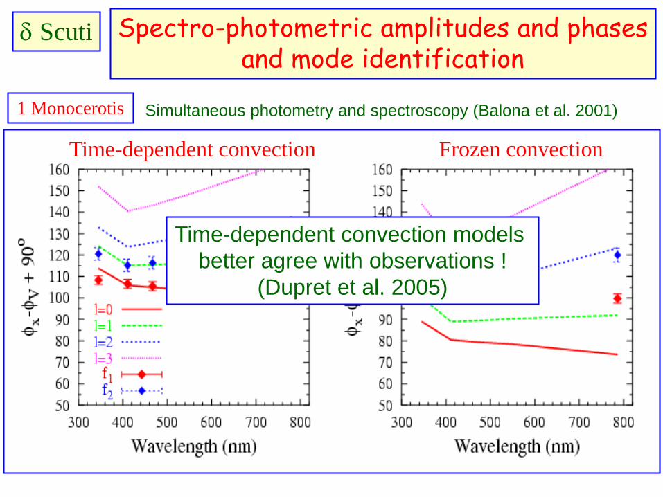
1 Monocerotis
Frozen convectionTime-dependent convection
Spectro-photometric amplitudes and phasesand mode identification
d Scuti
Simultaneous photometry and spectroscopy (Balona et al. 2001)
Time-dependent convection models
better agree with observations !
(Dupret et al. 2005)

Solar-type stars
A zoo of pulsating starswith very different physical characteristics
Pressure modes
Periods :3-8 min.
Large uncertainties
in the models of
coherent interaction
convection-oscillations

g Doradus
A zoo of pulsating starswith very different physical characteristics
Gravity modes
Periods : 0.3-3 days
Role of turbulent viscosity ?
Role of rotation ?

Classicalinstability strip
A zoo of pulsating starswith very different physical characteristics
Blue edge,
-mechanism (HeII): OK
Red edge : interaction
Convection-oscillations:
not fully understood

roAp
A zoo of pulsating starswith very different physical characteristics
High frequencies (4-20 Min.)
“-mechanism”
“H”-ionization zone
Very sensitive to the
eigenfunctions shape.
Role of magnetic field ?

CepheiSlowly Pulsating B
A zoo of pulsating starswith very different physical characteristics
-mechanism Fe M-shell
Possible constraints
on opacities,
Fe local abundances
Transport mechanisms
Subdwarf B

Red giants
A zoo of pulsating starswith very different physical characteristics
1) High amplitude Radial modes
2) Moderate amplitude radial and
non-radial modes excited by
turbulent motions.
Superb discovery
of COROT !!

White dwarfs
A zoo of pulsating starswith very different physical characteristics
DAV, DBV :Convective excitation
GW Virginis:−mechanism C-O K-shell
The blue edge location
depends on the Carbon and Oxygen abundances
The red edge depends onmass-loss-gravitational settling

Excitation mechanisms
• Instability strips
• Range of excited modes
(pressure or gravity modes ?)
Spectro-photometric
amplitude ratios
and phase-lags
Very useful for the
mode identification
Non-adiabatic oscillations

1. Excitation mechanisms
Self excitation
Stars as heat engines
Amplitude
until limit cycle reached
Cepheids, d Scuti, Cep, SPBs, g Dor, sdBs, …
• - mechanism
• Convective blocking
• mechanism
Stochastic excitation
Damped oscillation
+
Forcing term
(turbulent motions)
« Like a drum »
Solar-like oscillations
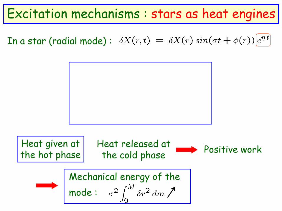
Excitation mechanisms : stars as heat engines
In a star (radial mode) :
Heat released atthe cold phase
Heat given atthe hot phase
Positive work
Mechanical energy of the
mode :

But … With homogeneous
chemical composition,
impossible to explain the
excitation of the modes.Charpinet et al. 2001
Main driving in the M-shell ionization zone of Fe
- mechanism : subdwarf B stars
damping
driving

Equilibrium between
radiative levitation and
gravitational settling
Fe
Fe
Fe
Charpinet et al. 2001
Fe
Diffusion time¿
Evolution time
Driving only possible if the
Fe is locally overabundant
at log T ~ 5.2
Thanks to radiative
levitation
Main driving in the M-shell ionization zone of Fe
- mechanism : subdwarf B stars

Huge number of
nodes in the core
Eigenfunctions similar
to classical p-modes in
the envelope
From Christensen-Dalsgaard (2004)
Acoustic structure of red giants and mode trapping

Seismic diagnostics from modes
trapped in the core
+ center
+ anticenterHe burning
CoRoT (Mosser et al. 2011)Kepler (Bedding et al. 2011)
Huge potential to probe the deepest layers :
- Determination of the evolutionary stage
- Measure of the He core mass (Montalban et al. 2012)
- Signatures of the -gradient in the core
H-shell burning
Period spacing :