STELLAR POPULATIONS FOUND IN THE CENTRAL KILOPARSEC …

STELLAR POPULATIONS FOUND IN THE CENTRAL KILOPARSEC OF FOUR LUMINOUSCOMPACT BLUE GALAXIES AT INTERMEDIATE z1

C. Hoyos,2

R. Guzman,3

A. I. DI´ıaz,

2,4D. C. Koo,

5and M. A. Bershady

6

Received 2007 February 20; accepted 2007 August 13

ABSTRACT

We investigate the star formation history of the central regions of four luminous compact blue galaxies (LCBGs) atintermediate redshift using evolutionary population synthesis techniques. LCBGs are blue (B� V � 0:6), compact(�B � 21:0mag arcsec�2) galaxies with absolute magnitudesMB brighter than�17.5. The LCBGs analyzed here arelocated at 0:436 � z � 0:525. They are among the most luminous (MB < �20:5), blue (B� V � 0:4), and high sur-face brightness (�B � 19:0 mag arcsec�2) of this population. The observational data used were obtained with theHubble Space Telescope (HST ) STIS, the WFPC2, and the first NICMOS camera. We have disentangled the stellargenerations found in the central regions of the observed targets using a very simple model. This is one of the first timesthis has been done for compact galaxies at this redshift using HST data, and it provides a comparison benchmark forfuture work on this kind of galaxy using instruments with adaptive optics in 10 m class telescopes. We find evidencefor multiple stellar populations. One of them is identified as the ionizing population, and the other corresponds to theunderlying stellar generation. The estimated masses of the inferred stellar populations are compatible with the dynam-icalmasses, which are typically (2 10) ; 109 M�. Ourmodels also indicate that the first episodes of star formation theseLCBGs underwent happened between 5 and 7 Gyr ago. We compare the stellar populations found in LCBGs with thestellar populations present in bright, local H ii galaxies, nearby spheroidal systems, and blue compact dwarf galaxies.It turns out that the underlying stellar populations of LCBGs are similar to yet bluer than those of local H ii galaxies.It is also the case that the passive color evolution of the LCBGs could convert them into local spheroidal galaxies if nofurther episode of star formation takes place. Our results help to impose constraints on evolutionary scenarios for thepopulation of LCBGs found commonly at intermediate redshifts.

Key words: galaxies: abundances — galaxies: evolution — galaxies: high-redshift — galaxies: stellar content

Online material: color figures

1. INTRODUCTION

Luminous compact blue galaxies (LCBGs) are luminous (MB

brighter than �17.5), blue (B� V � 0:6), and compact (�B �21:0 mag arcsec�2) systems experiencing an intense episode ofstar formation, with typical star formation rates (SFRs) rangingfrom 1 to 5M� yr�1. Although these SFRs are common in otherstarburst systems, the star formation episode takes place in a verysmall volume, allowing these compact objects to be seen fromcosmological distances. LCBGs are believed to contribute up to�50% of the SFR density in the universe at z � 1 (Guzman et al.1997). Their rapid evolution from those times until the presentday makes them responsible for the observed evolution of theluminosity function (Lilly et al. 1995), as well as the evolutionof the SFR in the universe.

Despite their importance, their relation to local galaxies is poorlyknown. The work presented in Guzman et al. (1997), Phillips et al.(1997), and Hoyos et al. (2004) gives a glimpse of the similarities

between LCBGs and local H ii and starburst nuclei populations.H ii galaxies are a subset of blue compact galaxies (BCGs) inwhich the spectrum is completely dominated by a component,present almost everywhere within the galaxy, resembling theemission of a H ii region (Sargent & Searle 1970). BCGs werefirst identified by Zwicky (1965) as faint starlike field galaxies onPalomar Sky Survey plates. BCGs often present an emission-linespectrum and a UV excess. Starburst nuclei were introduced inBalzano (1983); they show high extinction values, with very low[N ii] k6584/H� ratios and faint [O iii] k5007 emission. TheirH� luminosities are always greater than 108 L�. One of the mainingredients in any theory attempting to explain the final destinyof LCBGs is bound to be an accurate knowledge of the stellargenerations already existing in these distant sources. The sim-ilarities found between LCBGs and many local H ii galaxiesmake it possible that the star formation histories of both types ofobjects are very similar. Even though H ii galaxies were origi-nally thought to be truly young objects, experiencing their veryfirst star formation episodes (Searle & Sargent 1972; Sargent &Searle 1970), this hypothesis is no longer tenable after very deepCCD imaging of such objects (Telles & Terlevich 1997; Telleset al. 1997) or other very similar sources like the blue compactdwarf galaxies (BCDGs). BCDGs are similar to BCGs or H ii

galaxies but are an order of magnitude less luminous. The under-lying stellar populations of BCDGs are also older than thoseof BCGs (Papaderos et al. 1996a, 1996b; Loose & Thuan 1986),which show clear evidence of an older extended population ofstars. The properties of thismore extended component have beenfurther studied photometrically (see, e.g., Caon et al. 2005; Telleset al. 1997). The current view on local H ii galaxies is that they area mixture of three populations. The first of them is the youngest

1 Based on observations obtained with the NASA/ESA Hubble Space Tele-scope through the Space Telescope Science Institute, which is operated by theAssociation of Universities for Research inAstronomy (AURA), Inc., underNASAcontract NAS5-26555.

2 Departamento de Fısica Teorica (C-XI), Universidad Autonoma deMadrid,Carretera de Colmenar Viejo km 15.600, 28049 Madrid, Spain; [email protected], [email protected].

3 Bryant Space Science Center, University of Florida, Gainesville, FL 32611-2055, USA; [email protected].

4 On sabbatical at the Institute of Astronomy, Cambridge, UK.5 Department of Astronomy, University of California, Santa Cruz, CA 95064,

USA; [email protected] Department of Astronomy, University of Wisconsin, Madison, WI 53706,

USA; [email protected].

A

2455

The Astronomical Journal, 134:2455–2473, 2007 December

# 2007. The American Astronomical Society. All rights reserved. Printed in U.S.A.

population, responsible for the observed emission lines. The secondpopulation is an intermediate-age generation, older than 50 Myrbut younger than 1 Gyr. This population is unable to ionize theH i gas, and its luminosity is increasingly dominated by the con-tribution of giant stars and some asymptotic giant branch stars.The third population is the oldest one, older than 1Gyr. This pop-ulation generally dominates the stellar mass by a large factor, andit also occupies a larger volume.

The main target of this study is to characterize the stellar pop-ulations present in intermediate-redshift LCBGs by combiningthe spectral and color information available from these data withevolutionary population synthesis techniques. The modeled stel-lar populations are then compared to the stellar populations foundin H ii galaxies and the smaller yet similar BCDGs. It is alsointeresting to study the future evolution of the predicted stellarpopulations, to see whether they can become dwarf elliptical sys-tems (dE or Sph), as suggested by Koo et al. (1995) and Guzmanet al. (1998), or, alternatively, they can be the bulges of spiralgalaxies still in the formation process (Hammer et al. 2001;Kobulnicky & Zaritsky 1999; Guzman et al. 1998; Phillips et al.1997).

The observations and analysis techniques, together with thedifferent results they yield, are described in x 2. Section 3 pres-ents the data analysis. The models that have been constructed toexplain the observations are discussed in x 4. The LCBGs pre-sented in this work are compared to relevant samples of local gal-axies in x 5. The summary is given in x 6.

The cosmology assumed here is a flat universe with�� ¼ 0:7and �m ¼ 0:3. The resulting cosmological parameters are H0 ¼70 km s�1 Mpc�1 and q0 ¼ �0:55. Given these values, 100 corre-sponds to 1.8 kpc at z ¼ 0:1 and 5.8 kpc at z ¼ 0:45.

2. OBSERVATIONS AND DATA REDUCTION

In this paperwepresent long-slit spectra, deep opticalV (F606W)and I (F814W) images, and infrared F160Wimages of four LCBGs

with redshifts between 0.436 and 0.525. The data were obtainedusing the Space Telescope Imaging Spectrograph (STIS), theWFPC2, and the first NICMOS camera. Target names, redshifts,look-back times, B absolute magnitudes, exposure times, half-light radii, velocity dispersions, and virial masses within Re, aswell as an identifying numeral for the observed objects, aregiven in Table 1.The STIS long-slit spectra are imaged on a SITe 1024 ; 1024

CCD,with 0.0500 square pixels operating from�2000 to 110008.Several instrumental configurations were used. The instrumentalsetup used to observe objects 1, 3, and 4 used the low-resolutiongrating G750L. This instrumental setup provides a dispersionof 4.92 8 pixel�1, or about 190 km s�1 pixel�1, which in com-bination with a slit 0.500 wide gives a spectral resolution of about29 8 (FWHM). The spectral coverage provided by this setupis about 5000 8. The central wavelength is 7750 8. The higherresolution grating G750M was also used for objects 3 and 4.It provides a dispersion of 0.53 8 pixel�1, or about 35 km s�1

pixel�1. The slit width used was 0.200, thus giving a spectral reso-lution of about 2.1 8 (FWHM). The spectral coverage providedby this setup is about 500 8. These spectra are used to study thegas-phase velocity field, and the results from this work are pre-sented in Bershady et al. (2005). Object 2 was observed using thelower resolution grating G430M and the high-resolution gratingG750M. The G430M grating has a dispersion of 2.7 8 pixel�1,and the slit width used is 0.200. The central wavelength is 43008,and the spectral coverage is 28008. The data were reduced usingthe STSDAS7 package within IRAF.8 For a complete account ofthe reduction procedures and uncertainties and detailed descriptionsof the spectra, seeHoyos et al. (2004). It is worthmentioning that

TABLE 1

Log of HST STIS, WFPC2, and NIC1 Observations

Parameter SA57-7042 SA57-5482 SA57-10601 H1-13088

R.A.a................................................... 13 07 26.3 13 09 08.8 13 08 47.8 17 20 19.67

Decl.a.................................................. 29 18 25.7 29 15 57.7 29 23 41.1 50 01 04.7

STIS obs. date.................................... 2002 May 5 2002 Apr 9 2000 Jul 5 2000 Nov 6

G750L exp. time................................ 9898 . . . 4696 4932

G750M exp. time............................... 2760 18106 5571 5947

G430L exp. time................................ . . . 2790 . . . . . .

G430M exp. time............................... . . . 7709 . . . . . .WFPC2 F606W exp. time ................. 700 700 700 700

WFPC2 F814W exp. time ................. 900 900 900 1000

NICMOS F160W exp. time............... 2560 1280 5632 1792

Object ID ........................................... 1 2 3 4

z .......................................................... 0.525 0.453 0.438 0.436

tlook-back (Gyr)..................................... 5.2 4.7 4.6 4.5

MB ...................................................... �20.6 �20.8 �20.4 �21.1

Reb ...................................................... 1.4 1.5 1.9 2.4

mB ....................................................... 22.3 21.6 21.6 21.0

rec ....................................................... 0.25 0.29 0.36 0.47

Velocity disp. ( km s�1) ..................... 120 � 10 60 � 6 42 � 4 47 � 4

logM /M�d 10.7 10.1 9.7 9.8

Note.—All quantities given were calculated assuming q0 ¼ �0:55 and H0 ¼ 70 km s�1 Mpc�1.a Coordinates are given for equinox J2000.0. Units of right ascension are hours, minutes, and seconds, and units

of declination are degrees, arcminutes, and arcseconds.b Half-light radii in kiloparsecs.c Half-light radii in arcseconds.d Dynamical masses within Re calculated as in Hoyos et al. (2004). Uncertainties are 20%.

7 STSDAS is the Space Telescope Science Data Analysis System from theSpace Telescope Science Institute, operated for NASA by AURA, Inc.

8 IRAF is the Image Reduction and Analysis Facility, distributed by the Na-tional Optical Astronomy Observatory, which is operated by AURA, Inc., undercooperative agreement with the National Science Foundation.

HOYOS ET AL.2456 Vol. 134

STIS spectroscopic observations using the G750L and G750Mgratings are affected by fringing in the red end of the spectrum.This makes it necessary to use specially designed flats (called‘‘contemporaneous flats’’) in order to circumvent this issue. Theuse of this technique, which is implemented as a task withinSTSDAS, raises the signal-to-noise ratio (S/N) by around 15%.This is crucial for these observations. The proposal IDs for theseobservations are GO 8678 and GO 9126.

The images used were taken with theWFPC2, with the LCBGscentered in the Planetary Camera, a 800 ; 800 CCD, with 0.04600

square pixels. Two broadband filters were used, the F814W filterand the F606Wfilter. For each object and filter, two�400 s expo-sures were obtained, to allow for cosmic-ray rejection. The detailsof the reduction and analysis procedures can be found in Guzmanet al. (1998). The proposal ID for these data is GO 5994.

The infrared frames were obtained with the NIC1 camera ofNICMOS.9 This camera uses a low-noise, high quantum efficiency,256 ; 256 pixel HgCdTe array, with 0.043100 square pixels. The fil-ter used was the F160W, which has a bandpass of around 4000 8.For each object, several different exposures were collected andcombined to produce a final mosaic. The proposal ID is GO 7875.

The STIS data can only probe the central regions of these gal-axies because their outermost regions are too faint to be studiedspectroscopically with the Hubble Space Telescope (HST ). Spe-cifically, the STIS data can be used to study the line-emitting re-gion, where the starburst is taking place and most of the gas isionized. The line-emitting region of the observed galaxies has a ra-dius between 1.4 and 2.0 kpc. This is a little bit less than one effec-tive radius. On the other hand, theWFPC2 images and NICMOSframes are deeper, and the size of the observed galaxies in theimages is much larger than the size of the line-emitting region inthe STIS spectra. The analysis presented in this paper focuses onthis particular central region where the STIS spectra spatially over-lap with the WFPC2 images and NICMOS frames. This regionhas a radius of 1.7 kpc, on average.

3. RESULTS AND ANALYSIS

3.1. Emission-Line and Continuum Distribution

It is interesting to investigate whether the continuum distribu-tion and emission-line distribution differ in the STIS spectra. Thiswill help determinewhere the starburst has taken place. This infor-mation can be helpful in understanding the starburst triggeringmechanism and in constructing models for these objects. Herewe follow the analysis presented in Hoyos et al. (2004), although

it is given in a much simpler way. Furthermore, only objects 1and 2 are presented here, since the other two sources were dealtwith in Hoyos et al. (2004). The procedure is briefly reviewed.

Using the IRAF task fit1d, a ‘‘continuum frame’’ was made byfitting three cubic spline pieces to every line in the spectra; thena ‘‘line frame’’ was constructed by subtracting the continuumframe from the original two-dimensional spectroscopic frame.The spatial distribution of the continuum is obtained by column-averaging the whole continuum frame, and the spatial distribu-tions of the emission lines are obtained by column averaging theline frame over the columns that span 1.25 times the FWHM ofthe line. The spatial profiles for the two new objects studied aregiven in Figure 1.

Figure 1 shows the following:

1. The spatial distribution of the ionized gas and underlyingstellar population in object 1 is very similar to the distributionsobserved in objects 3 and 4 (Hoyos et al. 2004). The nebularcomponent light centroid does not coincide with the continuumcentroid, although the peaks of the different components clearlyline up. The two peaks observed at +1.5 and�2.7 kpc in the H�spatial profile are not real. This object is very similar to the com-etary BCDGs. In this particular case, the spread of the contin-uum is about twice the size of the line-emitting region. In theoptical images, this object shows a conspicuous tail and a verybright knot. It is also seen that the spatial extents of the two emis-sion lines used to trace the ionized gas are very similar.

2. For object 2, the differences in the centroid positions forthe continuum and the line-emitting region are very small whencompared to the spread of both. In this case, the ionized gas canbe said to lie in the center of the optical galaxy. This is to say thatthe line-emitting region coincides with the continuum light cen-troid. The true barycenter of these galaxies is not known. It isalso interesting to note that, in this particular case, the distribu-tions of each component are very noisy even for the continuum,and that the distributions of H� and [O iii] k5007 are very simi-lar to each other.

As in Hoyos et al. (2004), the H� and [O iii] k5007 lines werechosen to probe the ionized gas phase because [O iii] k5007 andH� are very close to each other in wavelength space, and there-fore they are affected by a similar extinction. For this reason,differences in their spreads can then reveal real differences intheir distributions, not just a reddening effect. As pointed out inHoyos et al. (2004), the observed differences in the spread of H�and H� or [O iii] k5007 and [O ii] k3727 can be accounted for bymoderate extinction, within the measurement errors, making itimpossible to detect extinction or excitation gradients unambig-uously. Finally, the inclusion of these two new objects in the

Fig. 1.—Continuum and emission-line spatial profiles. Only objects 1 and 2 are presented, since the spatial profiles for objects 3 and 4 are given in Hoyos et al.(2004). The S-axis is placed with respect to the slits depicted in Fig. 2. Increasing S corresponds to upper positions in that figure. The continuum is shown by the thicksolid line, [O iii] k5007 is shown by the thin solid line, and the dotted line represents H�.

9 Before the cryo-cooler was installed.

STELLAR POPULATIONS OF FOUR COMPACT GALAXIES 2457No. 6, 2007

sample of LCBGs with high-quality spatially resolved spectro-scopy allows us to give a first interval of the frequency of off-center10 starbursts in LCBGs. Since the result is that three out ofsix LCBGs with STIS spectroscopy happen to have their star-bursts displaced from their centers, all that can be said is that thefraction of LCBGs with shifted starbursts is 50%þ49%

�20%. More ob-servational work is needed to assess the frequency and impactof this issue in the evolution of LCBGs.

3.2. Line Ratios, Reddening, Equivalent Widths,and Metallicities

The observed flux of each emission line and the equivalentwidths have been measured via Gaussian fits using the STSDAStask ngaussfit, according to the method outlined in Hoyos et al.(2004). This task can fit to a set of x-y values the sum of a straightbaseline and one or several Gaussian profiles. This task also givesapproximate errors for the fitted parameters, calculated by resam-pling. The emission lines were fitted rather than summed becauseof residuals of bad pixels.

Two different positions are considered for each galaxy corre-sponding to the inner (a) and the outer (b) regions of each object.Despite these names, both the a and b regions defined here arewithin the line-emitting region. These two one-dimensional ex-tractions are defined so as to encompass approximately the sameline luminosity. It is in these two regions that the following stellarpopulation analysis is carried out. These apertures are near oneeffective radius for the line-emitting region, as detected through

the spectroscopic aperture. The linear sizes of both extractionsare given in the second row of Table 2, in kiloparsecs. For po-sition a, both the FWHM and central wavelength are left as freeparameters. However, for position b, the FWHM is fixed to theFWHM derived for position a to decrease the number of free pa-rameters and hence increase the goodness of the fit in poor S/Nconditions. The [O ii] k3727, H�, and both [O iii] lines can be ob-served in all cases. However, althoughH� is detected for object 4,it is affected by many bad pixels that render the line unusable.In the case of object 1, H� is detected, too.The amount of extinction is here parameterized using the

logarithmic extinction coefficient c (H�). It was derived usingstandard nebular analysis techniques (Osterbrock 1989) usingthe H� /H� Balmer line ratios. For object 1, the H� line was usedto derive the extinction coefficient, which agreed well with thatderived fromH� and H� but had a smaller uncertainty. Since theobserved galaxies are at high Galactic latitude, suffering Galacticextinctions ofAB < 0:11magwhich correspond to c(H�) < 0:05(Burstein & Heiles 1982; Sandage & Tamman 1974), it was as-sumed that all extinction occurs within the target objects. Thisapproximation is further validated by the fact that the incominglight is redshifted, and therefore the extinctionwill bemuch lower.Consequently, the spectra have been dereddened in the rest frameof the targets according to a standard reddening curve (Whitford1958), assuming case B recombination theoretical line ratios. Theuse of different extinction curves will not significantly change theresults, since they do not differ from the one used here in thewave-lengths of interest. The value of c(H� ) is determined indepen-dently for the inner and outer regions of all objects but H1-13088,10 Here the word ‘‘center’’ means the continuum light centroid.

TABLE 2

Absorption Coefficients, Dereddened Line Ratios, Rest-Frame Equivalent Widths, Oxygen Content, and Stellar Colors

Object 1 Object 2 Object 3 Object 4

Parameter Inner Outer Inner Outer Inner Outer Inner Outer

Size (kpc)................................................... 0.83 1.66 1.04 2.01 1.28 2.03 1.27 3.04

c(H�) ......................................................... 0.0 � 0.1 0.0 � 0.1 0.0 � 0.1 0.0 � 0.2 0 � 0.1 0.10 � 0.2 0.10 � 0.05 0.10 � 0.05

log (½O iii� kk4959; 5007)/H�................... 0.71 � 0.04 0.60 � 0.03 0.60 � 0.03 0.39 � 0.04 0.67 � 0.03 0.44 � 0.06 0.7 � 0.1 0.54 � 0.08

log (½O iii�/½O ii�)a ....................................... 0.48 � 0.04 0.38 � 0.02 �0.31 � 0.04 �0.38 � 0.05 0.43 � 0.06 0.33 � 0.09 0.28 � 0.09 0.26 � 0.07

log R23b....................................................... 0.83 � 0.04 0.75 � 0.02 1.08 � 0.02 0.92 � 0.06 0.80 � 0.03 0.61 � 0.05 0.89 � 0.08 0.73 � 0.06

logW½O ii� k3727c ........................................... 1.88 1.94 2.18 2.11 1.65 1.43 1.93 1.79

logWH�c ..................................................... 1.79 1.87 0.60 0.47 1.59 1.51 1.67 1.57

logW½O iii� kk4959þ5007c.................................. 2.51 2.53 1.10 0.77 2.28 2.00 2.40 2.13

logWH�c ..................................................... 2.00 1.82 . . . . . . 2.30 2.16 . . . . . .

NICMOS Fkd ............................................. 2.8 � 0.3 . . . 5.9 � 0.6 . . . 3.9 � 0.4 . . . 10 � 1 . . .

NICMOS luminosityd ................................ 2.7 . . . 3.9 . . . 2.4 . . . 7.0 . . .

12þ log (O/H)hie....................................... 8.4 8.5 7.8 8.1 8.4 8.7 8.2 8.5

12þ log (O/H)lof ....................................... 7.8 7.7 8.8 8.6 7.7 7.5 8.0 7.7

B� Vobsg .................................................... 0.41 0.49 0.28 0.27 0.08 0.25 0.26 0.35

B� Vstellarh ................................................. 0.13 0.20 0.34 0.33 �0.08 0.16 0.12 0.28

Notes.—In the first row the physical sizes of each aperture in linear kiloparsecs are given. For object 1, the logarithmic extinction coefficient was derived from theH�/H� ratio. Its value was consistent with the value derived using H�, but the error was smaller. For object 2, the [O ii] k3727 flux is first measured in the integratedG430L spectra. The intensities in each zone (a or b) are then derived by requiring that the zones emit 50% of the light each. This is true to within 5% for the other threelines seen in the other instrumental setup. The reported values of logW½O ii� k3727 also correspond to the integrated spectra. For object 4, H� is not observed and the listedvalue for the logarithmic extinction coefficient is an assumed value, typical for local H ii galaxies.

a This is defined as the reddening-corrected ratio [O iii] kk4959, 5007/[O ii] k3727. The other line ratios are also reddening-corrected.b R23 is defined as the reddening-corrected ratio (½O ii� k3727þ ½O iii� kk4959; 5007)/H�.c The rest-frame equivalent widths are in angstroms. The average error in the rest-frame equivalent width is 17%. This corresponds to an error of 0.07 in the loga-

rithm.Most errors fall in the 15%–20% interval. The G750M spectra used for object 2 bear the largest uncertainties, since the slit width used was 0.200 wide, compared tothe 0.500 slit used for the other three objects. The errors in the equivalent widths for object 2 are therefore 30%, corresponding to 0.13 in the logarithm.

d Units of Fk are 10�15 ergs s�1 cm�2. The reported luminosities are rest-frame luminosities in the rest-frame wavelength range that shifts to the F160Wwavelength

passband. The luminosity units are 1042 ergs s�1, and the errors are typically 15%. Both of these numbers refer to the total luminosity from the line-emitting region.e Oxygen abundance derived using the calibration for the upper branch (Pilyugin 2000). The solar value is 8.69 (Allende-Prieto et al. 2001).f Oxygen abundance derived using the calibration for the lower branch (Pilyugin 2000). The solar value is 8.69 (Allende-Prieto et al. 2001).g Observed colors. The uncertainty is 0.01 mag in all cases.h Rest-frame, stellar-population-only, extinction-corrected B� V colors. This is defined in the text. The uncertainty is 0.09 mag.


for which H� is unfortunately not well measured. A global valueof c(H� ) ¼ 0:1 � 0:05, typical for local H ii galaxies (Hoyos &Dıaz 2006), is adopted. No underlying stellar hydrogen absorp-tion is detected, as the continuum is very low.

Line equivalent widths were measured in the STIS spectra. Itis possible to measure the line equivalent widths, despite the factthat these spectra are emission-line-dominated, if the errors arecarefully estimated. This is explained in detail inHoyos et al. (2004),where it is also possible to see four examples of the extracted spectra(see Hoyos et al. 2004, Fig. 2).

Themeasured extinction coefficients and dereddened line ratiosare given in Table 2, together with the measured rest-frame equiv-alent widths. It is seen that the extinction values are always verysmall. It can also be seen that the ionization ratio log ½O iii�/½O ii�and both the log ½O iii�/½H ii� and log R23 numbers are alwayssmaller in the outer zones of the observed galaxies than in the innerpart of the line-emitting region. We define R23 as the reddening-corrected (½O ii� k3727þ½O iii� kk4959; 5007)/H� ratio. In somecases, the differences are larger than the derived errors, revealingthe existence of a gradient. For some other cases the differencesare more dubious. However, even though it is not possible toclaim that these gradients have been detected for all of the indi-vidual objects studied, the fact that these differences between thea and b zones hold for themajority of cases allows us to think thatthese gradients are real, at least for typical LCBGs.

3.3. The Oxygen Content and Metallicity Estimates

One of the main goals of any nebular analysis is to estimatethe metallicity of the emitting nebula. There are many reasons todetermine the metallicity of the ionized gas in a galaxy, but chiefamong them is that it yields an up-to-date determination of thechemical composition of the most recent generation of stars bornin the galaxy studied.

The emission-line spectrum from a star-forming region de-pends strongly on the electron temperature and metallicity of thenebula. The ratio of the auroral line [O iii] k4363 to the lowerexcitation lines [O iii] kk4959, 5007 gives a direct determinationof the electron temperature where O+ and O++ are the dominantspecies, but beyond certain metallicities, the increasing coolingleaves no energy to collisionally excite the upper levels.When thisis the case, one must resort to determining the oxygen abundanceempirically.

In principle, the oxygen content can be determined fromthe intensities of the optical emission lines using the R23 num-ber, defined as the reddening-corrected ratio (½O ii� k3727þ½O iii� kk4959; 5007)/H�. This method was originally devel-oped by Pagel et al. (1979; see also Pagel et al. 1980, Edmunds&Pagel 1984,McGaugh 1991, and Kewley&Dopita 2002, amongmany others). The main problem with this empirical method isthat the calibration is double-valued, and some a priori knowl-edge of the metallicity range is needed in order to solve this de-generacy. Since the S/N of the spectra used is not very large, noother lines that could help break this degeneracy are detected.Thus, the lack of this initial knowledge about the oxygen contentremains, and the metal content of the galaxies studied cannot becleanly determined. Instead, the metallicity values that resultfrom the use of the Pilyugin (2000) calibration for both the lowerand upper branches are calculated. The metallicity estimates cal-culated using the Pilyugin (2000) formulae are given in Table 2.Unfortunately, the measured values for log R23 squarely place ourobjects in the turnaround region of the 12þ log (O/H)- log R23

plot. In this regime, the only thing that can be safely said is thatthemetallicity is between 7.7 and 8.4. Therefore, the analysis canonly safely conclude that these LCBGs have an oxygen content

greater than 7.7 but lower than the solar value of 8.69 (Allende-Prieto et al. 2001). It is also worth mentioning that, with the avail-able data, it is not possible to unambiguously detect a gradient inthemetallicity of these objects, since the derived values of R23 im-ply that the oxygen content of both zones can lie in a very widerange.11 It can also be concluded that the R23 method is not best-suited to determining the gas-phase metallicity of LCBGs be-cause the R23 diagnostic is likely to fall in this regime.

However, one initial metallicity estimate can be provided bythe ratio [N ii] k6584/H�, as suggested by Denicolo et al. (2002).Since [N ii] k6584 cannot be measured in the spectra analyzedhere, as it is below the detection limit due to poor S/N, it is notpossible to use the spectra used here directly for this task. Theonly available information is the Guzman et al. (1996) W. M.Keck telescope [N ii] k6584/H� measurements for a set of verysimilar sources from the same parent sample. These measurementsconsist of very high quality spectra obtained using the HighResolution Echelle Spectrometer (HIRES). The average oxygencontent of the Guzman et al. (1996) sources, derived using theDenicolo et al. (2002) expression for 12þ log (O/H), is 12þlog (O/H) ¼ 8:6 � 0:1. This value is a little bit too high to becompletely compatible with the majority of the Pilyugin (2000)metallicity calculations presented above, although it is compat-ible with some of them. This indicates that the oxygen content ismuch more likely to lie in the upper half of the interval allowedby the oxygen line ratios. It is interesting to note that the HIRESmeasurements of [N ii] k6584/H� are all around 0.18, and thatthe 3 � detection threshold at H� is around 15% of H� for theSTIS spectra,meaning that the STIS spectra were very close to de-tecting the nitrogen line. This is true for both the low-resolutionand high-resolution configurations.

3.4. Scaling and Registering of the Data and Calculationof Stellar Colors and NIR Luminosities

In order to describe the stellar populations found in the galaxiesstudied, it is necessary to match the STIS spectroscopic frameswith theWFPC2 images and theNICMOS frames. This is done byforcing each galaxy’s centroid in the WFPC2 and NICMOS im-ages to coincide with the center of the continuum distribution ofthe STIS spectroscopic frames. Once both centroids are calculated,the slit orientation with respect to the image is used to determinewhat pixels in theWFPC2 frames correspond to the inner and outerzones defined previously for the STIS spectra.

Figure 2 shows the slit placement in the F814W and F606WWFPC2 images. The bidimensional spectra presented for objects1, 3, and 4 are low-resolution G750L frames, while the spectrumpresented for object 2 is a high-resolution G750M frame. In thisfigure, the spectra have been scaled and approximately alignedwith the images. It is seen that the STIS spectra only probe themost luminous regions of the observed objects, corresponding tothe line-emitting region. This area spans less than 100, and it hasbeen further divided into two regions. This makes it necessary touse the spatial resolution of the HST instruments. Even thoughthese objects have been observed from the ground in the UBRIKbands, it is not possible to merge those data with the observationspresented here because the spatial resolution of those observa-tions is not high enough to study the presented objects at the sub-arcsecond level. The stellar population analysis presented in thefollowing section is therefore best suited for the volume withinthe line-emitting regions of the studied galaxies. This region typ-ically has a radius of 1.7 kpc.

11 In addition, the metallicity gradients of compact systems are likely to beintrinsically small because of the mixing.


Figure 3 shows the NICMOS frames. Each panel is 2.500 on aside. Again, the images have been rotated so that the slit silhouetteis vertical, as shown in the figure. It is seen that the STIS spectrafocus on the very central regions of the objects.

The next step is to determine the B� V color of the areas inthe WFPC2 F814W and F606W images that match the inner (a)and outer (b) zones of the STIS spectra. In order to accuratelydetermine said color, several issues must be taken into account.The first of them is to correct the integrated DN (CCD counts) ineach area for the imperfections of the charge transfer mechanism.There are several options to accomplish this task. The version usedin the WFPC2 Instrument Handbook, based on the 2002 May 31version of A. Dolphin’s calculations, was used. This correctiondepends on the objects’ location in the CCD. It also depends onthe objects’ accumulated DN and CCD gain. This correction is

obviously insensitive to the filter used. Fortunately, for the ob-servations used, any given galaxy is always imaged in the sameCCD location, and the accumulated counts are very similar forthe two filters used. This correction is therefore very small. It onlychanges the observed colors by less than 0.1 mag, usually muchless. The statistical error introduced by this correction was esti-mated by varying the DN parameter of the software tool previ-ously mentioned around the observed DN number. It turned outthat the magnitude error introduced by this correction was neg-ligibly small, 0.001mag in the worst case. For a complete reviewof this problem and the different approaches to correct for it, seeDolphin (2000).The second issue is the derivation of the k-correction. This

step is needed to convert from the observed I � V colors to therest-frame B� V colors. The fits given in Fukugita et al. (1995)for the case of an irregular Magellanic spectrum are used. Thek-corrections are 0.32 for objects 3 and 4, 0.39 for object 2, and0.47 for the furthest object. The errors introduced by this correc-tion are mainly systematic, arising from deviations of the realgalaxy spectra from the assumed Irr spectrum. These are estimatedto be around 0.08 mag, as was done in Guzman et al. (1998).The third issue is to derive the emission-line-free colors. The

method presented in Telles & Terlevich (1997) is adopted. Thismethod uses the rest-frame equivalent widths, together with theB and V filter transfer functions, to estimate the contribution ofthe emission lines to the observed galaxy colors. The method isnow sketched. Given an observed color A� B, it can be writtenas

B� A ¼ CBA � 2:5 logLcB þ LlBLcA þ LlA

; ð1Þ

whereCBA is the photometric constant, LcX is the continuum lumi-nosity in the X band, and LlX is the line luminosity falling withinthe X band.If the line luminosities are considered to be small perturbations

to the spectrum, the above equation can be cast into the followingform:

B� A ¼ (B� A)0 þ 1:086 LlA=LcA � LlB=L

cB

� �; ð2Þ

Fig. 2.—Matching between the STIS two-dimensional spectra and theHST WFPC2 images. Each spectral strip spans 2.500 in the spatial direction. The linear scale isgiven for each object in the figure. Each spectral strip spans 700 8 except for object 2, in which the wavelength coverage is given in each image. The spectral stripspresented for these objects are not registered with respect to the spectral strips shown for the other objects for this reason. The H� strip for object 1 is not perfectlyregistered with respect to the H� strips for objects 3 and 4 because the H� line fell very near the CCD edge. This spectral strip still spans 700 8, however. The slitorientation is shown superimposed on HST F606Wand F814W images which are 2.500 on a side. It is interesting to note that the spatial distribution of the continuum islopsided with respect to the peak. This is most evident in objects 3 and 4.

Fig. 3.—NICMOS F160W reduced images. Each postage stamp is 2.500 on aside. The slit is placed as in Fig. 2. The number in the upper left corner of eachpanel corresponds to the identifying numeral of Table 1.


where (B� A)0 is the color that would be observed in the absenceof the emission lines.

It is also possible to write the color correction as

A� B ¼ (A� B)0 þ 1:086LlA

IAWA

� LlBIBWB

� �; ð3Þ

where WX is the bandpass of the X band and IX is the averagespecific intensity.

The color correction can therefore be written as

1:086

PAiEW(i )

WA

�P

BiEW(i )

WB

� �; ð4Þ

where EW(i) is the line equivalent width of the ith emission lineand Xi is the filter transfer function evaluated at that wavelength.

It is important to note that, even if the line equivalent widthsused in the above formulae bear large uncertainties, any error inthe measured equivalent widths is greatly diminished or canceledout. This happens because the same equivalent width appears inboth terms of the color correction with opposite signs, althoughwith possibly different multiplicative factors.

The applied corrections range from essentially zero to 0.25mag.The statistical error introduced by this correction is very small.Given the derived uncertainties in the measured equivalent widths,these errors are less than 0.02 mag.

Finally, the E(B� V ) color excess is derived from the c(H� )values for each zone. These color excesses are very small andvirtually error-free. The resulting colors are therefore rest-frame ,stellar-population-only, extinction-corrected B� Vcolors. Thetotal photometric errors, obtained by adding in quadrature all theaforementioned uncertainties, are estimated to be 0.09 for all ob-jects. These colors are gathered in Table 2 for the inner and outerparts of the line-emitting region in which the stellar populationsare studied.

The NICMOS data were used to calculate the total F160Wluminosities of the line-emitting regions. It is necessary to usethe NICMOS data in this way because of the larger angular ex-tent of the NICMOS point-spread function, which makes it im-possible to calculate the observed fluxes of the a and b zonesseparately with the same accuracy as for the optical frames. Themeasured fluxes and luminosities are gathered in Table 2. Thereported luminosities all assume c(H� ) ¼ 0:2, and they also as-sume that AX /AV ¼ 0:4, where AX is the extinction in the wave-length range that maps into the F160W passband. This value isthe average value for that ratio between the I and J bands. Thecontribution from the nebular continuum, which begins to beimportant at these wavelengths, has been estimated at less than oraround 10%using the standard techniques presented inOsterbrock(1989).

It is seen in Table 2 that the colors of the inner zones areusually bluer than those of the outer zones of the line-emittingregion, in accordance with the Guzman et al. (1998) color pro-files. This can be interpreted in light of the results presented inx 3.2. Whenever one region in a galaxy is redder than anotherregion, it can be caused by differences in reddening, metallicity,or age. The first of these factors is unlikely to play a role in thisparticular case, since the reddening has been estimated, and it isvery small. The second factor is also unlikely to be responsiblefor the observed color gradients, since the metallicity differencesare likely to be very small in these systems at such short spatialscales because of very efficient mixing by supernova-driven winds.

Moreover, we conclude that the observed color differences betweenthe a and b zones are more likely to arise from age differencesbetween these two zones. Specifically, the underlying stellar pop-ulations in the b zones are typically older than the stellar pop-ulations of the a zones of their respective galaxies. The chemicalenrichment histories of both regions have probably been very sim-ilar for the reasons outlined above. This is an important finding forthese distant and compact sources.

Alternatively, it might be possible to think that the color gra-dient is caused by mass segregation. If, for instance, most of thenewly formed ionizing stars were in the a zone, the color of theinner part would be naturally bluer than the color of the outer zone.This scenario could also explain the observed differences in theionization ratio between the two zones, which would be higher inthe inner zone because of the higher amount of ionizing photonsavailable to ionize the inner parts of the nebula. Although masssegregation is a concern for massive clusters (see, e.g., Stolteet al. 2005 and de Grijs et al. 2002), it only operates at very shortdistances (10 pc at most), and not at the much larger scales ofinterest in the present case. The possibility of a spatially varyingpresent-day mass function can then be safely ruled out.

4. THE EVOLUTIONARY MODELS

The observational data gathered for the LCBGs presented herecan be used to construct galaxymodels that represent the objects.Although the models presented are very crude and tailored, theyprovide at least an idea of the stellar inventory and possible evo-lution of these LCBGs. This will shed light on the possible evolu-tion and age of these galaxies. In this section, the star formationhistory of the four LCBGs is studied using evolutionary popula-tion synthesis techniques. The models have been built using theBruzual & Charlot (2003) and Leitherer et al. (1999) evolutionarymodels. For each galaxy and extraction, a or b, two simple stellarpopulations are combined. One population is designed to mimicthe observed properties of the ionizing stellar population, and theother is chosen tomatch the observed colors when combined withthe ionizing population. This latter population therefore representsthe underlying population. We note that the population analysisused here is carried out for both the inner and outer zones of theline-emitting region separately, taking advantage of theHST spa-tial resolution. In addition, the fact that the star-forming region issplit into two subregions can also help to model possible delaysbetween the star formation episodes in the inner zone and in theouter zone of the line-emitting region.

The metal content of the ionizing stellar population is as-sumed to be equal to the metal content of the ionized gas. Sincethe only information available on the metal content of the ioniz-ing population of these sources comes from the gas-phase oxygenabundances,12 two sets of models are constructed. Model set 1assumes that the ionizing population has a metallicity of Z ¼0:008. Model set 2 adopts Z ¼ 0:004 for the metal content of theionizing population. These two numbers can be mapped into12þ log (O/H) ¼ 8:4 and 8.0, approximately, assuming solarchemical proportions. Therefore, for each galaxy and extraction,two models of different metallicities are built. The stellar inven-tory of the observed galaxies is described according the follow-ing steps:

1. The first step is the derivation of the masses of the ionizingpopulations.

12 The value of 12þ log (O/H) lies between 7.8 and 8.4, although the pre-ferred value is 8.4 because of the Guzman et al. (1996) HIRES measurements.


2. The second step is the determination of the ages and colorsof the ionizing populations. In this step the Leitherer et al. (1999)models are used.

3. In the third step the mass of the underlying stellar pop-ulation is derived, together with its age. The Bruzual & Charlot(2003) models are used to represent the older stellar generation.

4. The last step is a double-check of the derived masses usingthe measured NICMOS luminosities.

4.1. The Mass of the Ionizing Population

The mass of the ionizing population is a very important pa-rameter that defines it. If the mass of the ionizing population ishigh enough, the initial mass function (IMF) will be well sam-pled. If the IMF is not well sampled, it might be the case that themodels cannot be used to describe the stellar population. This ef-fect is commonly known as the ‘‘richness effect,’’ or the ‘‘Poissonshot noise.’’ Depending on the slope and cutoff masses of theIMF used, this can become a problem for population masseslower than 105M�, but for the usual Salpeter IMF the mass limitis lower. This issue has been extensively studied in the series ofpapers by Cervino et al. (2000, 2001, 2002).

The mass of the ionizing population,M�, can, in principle, bederived from the luminosities of the observed recombination linesaccording to the following considerations. As the stellar popula-tion ages, the number of hydrogen-ionizing photons per unit massof the ionizing population also decreases. Assuming that the ageof the ionizing population is related to the intrinsicWH�, a relationshould exist between the number of hydrogen-ionizing photonsper unit mass of the single stellar generation andW�. Such a rela-tion is given for single-burst models in Dıaz et al. (2000b). Theexpression used is

log Q(H)=M�½ � ¼ 44:8þ 0:86 logWH�; ð5Þ

where Q(H) is the number of hydrogen-ionizing photons persecond, M� is expressed in solar masses, and WH� is the ‘‘in-trinsic’’ equivalent width, the one that would be observed if nounderlying stellar population were present. Again, this expres-sion works best in stellar populations with well-sampled IMFs.The number of ionizing photons is an integral over the massrange more affected by the richness effect, and it is therefore verysensitive to small number statistics when applied to low-masspopulations. The IMF used to derive this expression had an ex-ponent of 2.35, a lower mass limit of 0.85M�, and an uppermasslimit of 120 M�.

However, the presence of the underlying stellar populationintroduces a degeneracy in the measurements of the equivalentwidths. This prevents us from measuring directly the equivalentwidths that would be observed if only the ionizing stellar pop-ulation were present. The main goal of the stellar populationanalysis presented here is then to unravel the different stellar pop-ulations. This is carried out following the ideas presented in Dıazet al. (2000a). In order to solve this degeneracy in equivalent widthintroduced by the presence of the underlying population, the up-per envelope of the relationship between logWH� and log (½O iii�/½O ii�) presented in Hoyos & Dıaz (2006, Fig. 6) was used toestimate the equivalent width that would be observed in the ab-sence of a previous stellar generation. This ‘‘effective’’ equiva-lent width is calledW 0

� . This assumption is now briefly justified.

In theWH�-to-½O iii� kk4959þ 5007/½O ii� k3727 ratio diagramfor very luminous H ii galaxies, if the observed range of ion-ization degrees is ascribed to the age of the ionizing population,it is reasonable to assume that the vertical scatter shown by the

data is caused by different contributions of continuum light fromthe underlying population.13 The expression used is

logW 0eA; � ¼ 2:00 � 0:02þ (0:703 � 0:028) log ½O iii�=½O ii�:

ð6Þ

The upper envelope of this relation, which defines the ‘‘effec-tive’’ equivalent width, is then relevant to estimate the ‘‘intrin-sic’’ equivalent width because the objects located on top of thisupper envelope are likely to be the ones in which the underlyingpopulation contribution isminimal. This effective equivalentwidthallows us to estimate themass of the ionizing population assumingthat W 0

� is equal to the real, or intrinsic, equivalent width thatwould be measured if the starburst could be observed in isola-tion. This is done via the expression given above using the mea-sured H� luminosities to obtain the number of hydrogen-ionizingphotons per second through standard nebular analysis techniques(Osterbrock 1989). The resulting stellar masses of the ionizingpopulation are given in Table 3. Typical ionizing populationmassesrange from 8 to 30 millionM�. The systematic errors affectingthese calculations are explained in the following paragraphs.The effective equivalent widths, which are mostly in the 100–

200 8 interval, are still lower limits only to the real value of theequivalent width, because the empirical method used here to de-rive the former does not forbid the existence of objects with higherobserved equivalent widths for their observed ionization ratio[O iii]/[O ii]. This is indeed a possibility, since the work presentedin Hoyos & Dıaz (2006) used local galaxies, and the galaxiesanalyzed here are intermediate- redshift sources. Therefore, thederived value for the mass of the ionizing populations obtainedusing Q(H) (or, rather, the H� luminosity) and W 0

� can only belower limits to the real masses. It has to be said, however, that thepossible differences between the intrinsic and the derived effec-tive equivalent widths cannot be very high. The maximum attain-able equivalent width, which corresponds to the case in whichonly the nebular continuum is considered, is 1000 8. When thestellar continuum is taken into account, the maximum equivalentwidth drops to about 400 8, depending on the IMF, metallicity,and age of the population, and the largest H� equivalent widthsever measured are close to this latter quantity. This implies thatthe intrinsic equivalent widths of the observed starbursts haveto be in the 200–400 8 range. These considerations allow us toestimate the possible systematic errors introduced by this ap-proximation. Using the typical effective equivalent width and anaverage value for the maximum intrinsic equivalent width, thereal masses of the ionizing populations could be up to a factor of2 larger. However, even if the intrinsic value could be observedor somehow derived, the mass of the ionizing component ob-tained would always remain a lower limit because some photonscould actually be escaping from the nebula, and dust globuleswill always be present amid the gas clouds. Moreover, if theionizing population turned out to emit more photons harder than1 ryd than the number predicted by the models used to deriveequation (5), the mass would be underestimated, too. The newGenevamodelswith rotation at lowmetallicity (Maeder&Meynet2001) point in this direction. For these reasons, further steps

13 There is, however, a metallicity effect. In the absence of an underlyingstellar population, H ii galaxies with higher metallicity cloudswill present a lowerionization ratio due to lower effective temperatures of their ionizing stars.However, there will be no change in the equivalent width of H�, to zeroth order.Therefore, W 0

� should be a function of both the ionization ratio and metallicity.Only the ionization ratio dependence of the ‘‘effective’’ equivalent width is usedhere.

HOYOS ET AL.2462

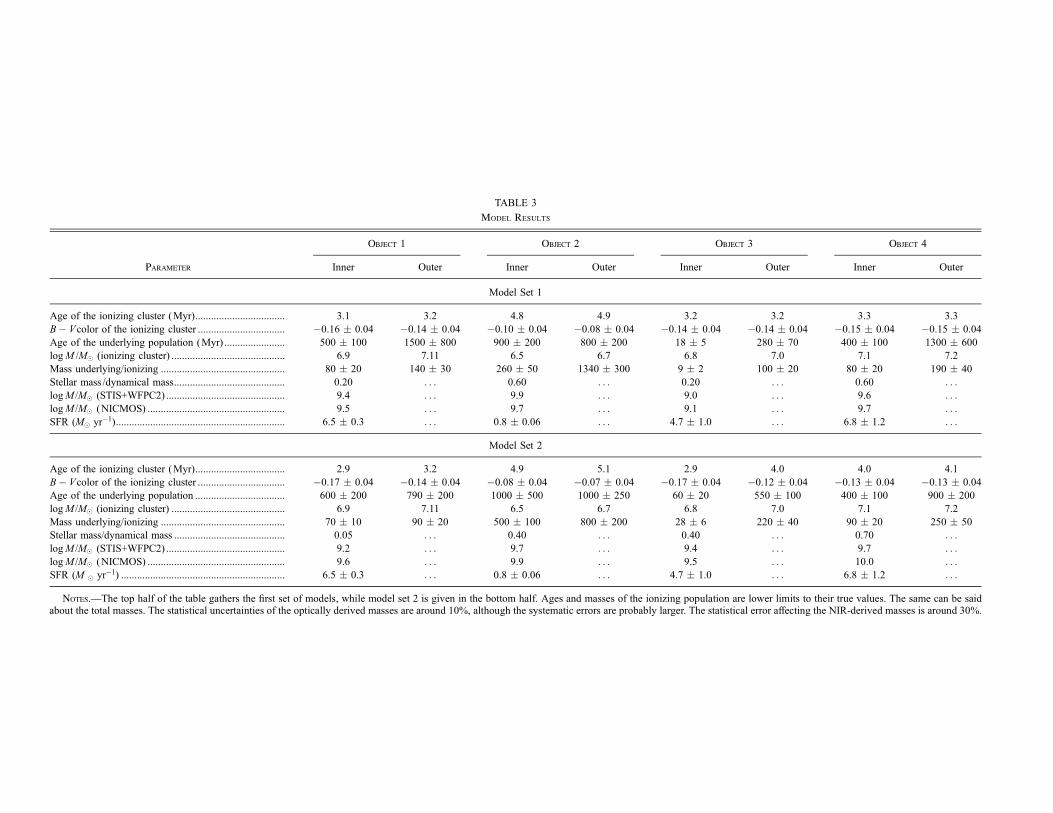
TABLE 3

Model Results

Object 1 Object 2 Object 3 Object 4

Parameter Inner Outer Inner Outer Inner Outer Inner Outer

Model Set 1

Age of the ionizing cluster (Myr).................................. 3.1 3.2 4.8 4.9 3.2 3.2 3.3 3.3

B� Vcolor of the ionizing cluster ................................. �0.16 � 0.04 �0.14 � 0.04 �0.10 � 0.04 �0.08 � 0.04 �0.14 � 0.04 �0.14 � 0.04 �0.15 � 0.04 �0.15 � 0.04

Age of the underlying population (Myr) ....................... 500 � 100 1500 � 800 900 � 200 800 � 200 18 � 5 280 � 70 400 � 100 1300 � 600

logM /M� (ionizing cluster) ........................................... 6.9 7.11 6.5 6.7 6.8 7.0 7.1 7.2

Mass underlying/ionizing ............................................... 80 � 20 140 � 30 260 � 50 1340 � 300 9 � 2 100 � 20 80 � 20 190 � 40

Stellar mass /dynamical mass.......................................... 0.20 . . . 0.60 . . . 0.20 . . . 0.60 . . .logM /M� (STIS+WFPC2) ............................................. 9.4 . . . 9.9 . . . 9.0 . . . 9.6 . . .

logM /M� (NICMOS) .................................................... 9.5 . . . 9.7 . . . 9.1 . . . 9.7 . . .

SFR (M� yr�1)................................................................ 6.5 � 0.3 . . . 0.8 � 0.06 . . . 4.7 � 1.0 . . . 6.8 � 1.2 . . .

Model Set 2

Age of the ionizing cluster (Myr).................................. 2.9 3.2 4.9 5.1 2.9 4.0 4.0 4.1

B� Vcolor of the ionizing cluster ................................. �0.17 � 0.04 �0.14 � 0.04 �0.08 � 0.04 �0.07 � 0.04 �0.17 � 0.04 �0.12 � 0.04 �0.13 � 0.04 �0.13 � 0.04

Age of the underlying population .................................. 600 � 200 790 � 200 1000 � 500 1000 � 250 60 � 20 550 � 100 400 � 100 900 � 200

logM /M� (ionizing cluster) ........................................... 6.9 7.11 6.5 6.7 6.8 7.0 7.1 7.2

Mass underlying/ionizing ............................................... 70 � 10 90 � 20 500 � 100 800 � 200 28 � 6 220 � 40 90 � 20 250 � 50

Stellar mass/dynamical mass .......................................... 0.05 . . . 0.40 . . . 0.40 . . . 0.70 . . .

logM /M� (STIS+WFPC2) ............................................. 9.2 . . . 9.7 . . . 9.4 . . . 9.7 . . .

logM /M� (NICMOS) .................................................... 9.6 . . . 9.9 . . . 9.5 . . . 10.0 . . .

SFR (M � yr�1) .............................................................. 6.5 � 0.3 . . . 0.8 � 0.06 . . . 4.7 � 1.0 . . . 6.8 � 1.2 . . .

Notes.—The top half of the table gathers the first set of models, while model set 2 is given in the bottom half. Ages and masses of the ionizing population are lower limits to their true values. The same can be saidabout the total masses. The statistical uncertainties of the optically derived masses are around 10%, although the systematic errors are probably larger. The statistical error affecting the NIR-derived masses is around 30%.

toward the determination of the intrinsic equivalent width fromthe effective equivalent width were not taken, and both quantitiesare assumed to be equal.

4.2. Determination of the Age and Intrinsic Colorof the Ionizing Population

The value of the effective equivalent width can be used to ob-tain more information about the underlying stellar populationsvia the Leitherer et al. (1999) models, making some assumptionsabout the metallicity and IMF of this stellar generation. Again,the effective equivalent width allows us to estimate, or at least toplace significant lower limits on, the age and intrinsic color ofthe ionizing population, assuming thatW 0

� is equal to the real orintrinsic equivalent width that would bemeasured if the starburstcould be observed in isolation. The Leitherer et al. (1999)modelsare used now.

Figure 4 presents nine models from the Starburst99 (Leithereret al. 1999) library that represent the evolution in the logW� ver-sus B� V plane of a single stellar population from its birth untilit is 10 Myr old. The nebular continuum emission is included inthese diagrams. This evolution is shown by the solid lines in thefigure. Ages increase from top to bottom. Three different met-allicities and IMFs are presented, as indicated in the figure. ThederivedW 0

� for both the inner and outer zones of the line-emittingregions of the observed sources is plotted against the emission-line-free, reddening-corrected color in the case of the studiedLCBGs. This is the color that would be measured if the starscould be observed in isolation.

It is interesting to note that the values of the effective equiv-alent width are close to the maximum equivalent width value ofthe plotted curves, which is the maximum value of the intrinsicequivalent width for zero-age clusters of the corresponding met-allicity and IMF,14 further highlighting the fact that, even thoughthe effective equivalent width is a lower limit to the real value,it is a reasonable approximation to it, especially if one considersthat, even if the real value could be somehow known, it wouldstill yield lower limits to the mass of the ionizing clusters becauseof photon escape and dust issues. It is clearly seen that three-fourths of the regions studied require the presence of an under-lying stellar population, since they do not lie along a solid line.Therefore, they cannot be reproduced by a single stellar popula-tion. It is also seen that the single stellar populations with a trun-cated Salpeter IMF have maximum intrinsic equivalent widthswhich are lower than the derived values ofW 0

� for many regions.This means that we can rule out these models as descriptions ofthe ionizing stellar populations found in the observed LCBGs,since the effective equivalent widths are in any case only lowerlimits to the real ones. This can be interpreted in the sense that theobserved galaxies have ionizing populations somassive that theyfully sample their respective IMFs, which is a necessary condi-tion to achieve high equivalent widths. In addition, the modelswhose IMFs have a slope of 3.33 are redder than the inner regionof object 3, which makes it impossible to accommodate an olderand redder underlying population in this model, and there are

Fig. 4.—Evolution of a single stellar population in the logWH�-(B� V ) plane from t ¼ 0 to t ¼ 10Myr. The data were taken from the Leitherer et al. (1999) library.In all cases, an instantaneous burst is assumed, and the nebular continuum emission is taken into account. Two different oxygen contents (Z ¼ 0:008, model set 1,bottom panels; Z ¼ 0:004, model set 2, top panels) and three different IMFs (Salpeter 1.0–100M�, left panels; power lawwith an exponent� ¼ 3:3with the same masslimits,middle panels; Salpeter IMF truncated at 30M�, right panels) are plotted. For the LCBG points,W 0

� is plotted against the emission-line-free, reddening-correctedcolor. The horizontal error bars represent the 0.09 mag uncertainty, and the vertical semierror bars reach to the observed equivalent width, in order to indicate the im-portance of the contribution of the underlying stellar population to the optical light. The filled circles represent the 0, 2, 4, 6, 8, and 10 ; 106 yr checkpoints. Object 1 isrepresented by half-filled squares, object 2 is represented by open circles, object 3 is represented by pentagons, and crosses denote object 4. Two symbols are shown foreach object, corresponding to the a and b extractions. In all cases, the b apertures have redder colors.

14 About 350 8 for the presented cases.


also some regions with W 0� greater than the zero-age equivalent

width of thosemodels. Themodels with Salpeter IMFs are there-fore chosen to describe the ionizing populations, simply becausethey are compatible with all these restrictions. Although the rea-sons to discard them�3:33 IMF are of course weaker, consideringmultiple IMFs is by nomeans justified given the few input data atour disposal. The use of the Salpeter IMF provides a crude yetconsistent description of the ionizing population found in the ob-served regions.

Assuming that W 0� equals the real equivalent width, as was

done before, and using the Salpeter IMF for the two metallicitiesthat correspond to the metallicities of the two model sets used, itis possible to calculate the ages and intrinsic colors of the ion-izing population. They are given in Table 3. The ionizing clustersare found to be very young ( less than 5 Myr in most cases). Asbefore, the use of the effective equivalent width instead of theunknown intrinsic value introduces a systematic error in the agedeterminations. The ionizing populations are then bound to beeven younger than the presented quantities. When dealing withvery young coeval single stellar populations, it has to be keptin mind that the observed properties of such populations do notchange to a great extent until they are about 3 Myr old, simplybecause of the fact that this is the minimum lifetime of even themost massive stars, and also because the approximation of aninstantaneous burst might fail at such short timescales. The mainconclusion is that the ionizing populations of the observed re-gions are probably extremely young. The systematic error in theintrinsic color of the ionizing population is also estimated fromthe color scatter of themodels used between zero age and themax-imum age allowed by the observedW 0

� . All errors are 0.04 mag.

4.3. The Age and Mass of the Underlying Population

The next step in describing the stellar populations found in theobserved LCBGs is calculating the age and initial mass of theunderlying stellar population. The single stellar populations usedto describe the underlying generation of stars are chosen from theBruzual & Charlot (2003) library. The evolutionary tracks usedare the 1994Padova ones, and the IMF chosen is the Salpeter IMF.The metallicity of this underlying stellar population is Z ¼ 0:004for the case of model set 1 and Z ¼ 0:0004 for the case of modelset 2. These are lower than the metallicities used to describe theionizing populations. In this step, the ionizing cluster is repre-sented by the single stellar population available in the Bruzual &Charlot (2003) library that most closely resembles the Leithereret al. (1999) model used before in terms of metallicity, IMF, andW 0

� -derived age.Assuming that the metallicities of the ionizing populations are

higher than the metallicities of the underlying populations triesto emulate the chemical evolution of the observed galaxies fromtheir inception until the onset of the observed starbursts. Althoughthe choice adopted is not justified by the use of any particularchemical evolution model, it is at least a zeroth-order solution tothe problem, since the Bruzual & Charlot (2003) models onlyoffer a limited array of metallicities for the different single stel-lar populations. In the framework of the closed-box model andthe instantaneous recycling approximation, the correspondinggas consumption fractions for the required metal enrichments are10% for model set 1 and 60% for model set 2, assuming zerometallicity in the distant past, before the starbursts that gave birthto the underlying stellar generations took place. The gas consump-tion fraction is larger in the metal-poor models, since the differ-ence in metallicity between the two simple populations mixedto construct them (Zion ¼ 0:004, Zunder ¼ 0:0004) is much largerthan the metallicity difference of the two simple populations

combined for the first models (Zion ¼ 0:008, Zunder ¼ 0:004).The yields provided byM.Molla (2006, private communication)and Maeder (1992) were used in these latter calculations. Al-though these estimates, by themselves, do not prove that thispicture is accurate to describe the star formation history of theseobjects, they show that the assumed metallicity differences be-tween the stellar populations used to build the models are at leastpossible. In addition, it has to be kept in mind that the globalremaining gas fraction is bound to be lower for the metal-richmodels in the framework of the closed-boxmodel and the instan-taneous recycling approximation than for themetal-poormodels.In particular, given the assumed metallicity for the ionizingpopulation of the second set of models, the gas consumptionfractions of pristine gas have to be higher than 60% in both cases,again in the closed-box model with the instantaneous recyclingapproximation.

The age and mass of the second stellar population are thenchosen so that the predicted equivalent width by the time thecurrent starburst is observed matches the measured equivalentwidth and the total color equals the calculated rest-frame, stellar-population-only, extinction-corrected B� V color. In essence,this procedure estimates the amount of ‘‘red light’’ that has to beadded to the ‘‘blue light’’ of the ionizing population in order tomatch the two observables available (B� V color and measuredH� equivalent width) at the time in which the observed starbursttakes place. This second stellar population is therefore designedto match the older stellar population.

The difference between the observed B� V color and the pre-viously derived intrinsic B� V color of the ionizing population(given in Table 3) can be approximately matched with ‘‘howred,’’ and the difference between the observed equivalent widthand the intrinsic equivalent width roughly translates into ‘‘howmuch’’ red light has to be added, although both quantities are ofcourse interlaced.

The errors in the observed equivalent widths (typically 17%)and stellar colors (0.09 mag, as estimated above) translate them-selves into errors in the relative mass of the underlying stellarpopulation with respect to the ionizing population and age. Al-though it is not true that 100% of the error in the relative masscomes from the uncertainties in the measured equivalent widthand that 100% of the error in the age of the underlying stellarpopulation arises from the errors in the derived stellar colors,15

these are the main dependencies. Assuming that this simplifiederror scheme holds, the typical uncertainties in the relative massof the ionizing cluster with respect to the mass of the ionizingcluster are 20%. The uncertainties in the age of the underlyingpopulation are 25% for ages below 109 yr and twice this amountfor older ages. This is because of the flattening in the B� V-agerelationship of the Bruzual & Charlot (2003) models. The resultsare also presented in Table 3.

4.4. NICMOS NIR Photometric Masses

The final step in this crude description of the stellar popula-tions found in the observed LCBGs is made possible by the useof NIR data. This information is now employed to check the like-lihood of the derived stellar populations by using the total lumi-nosities emerging from the line-emitting regions in the wavelengthrange that transforms into the F160W wavelength interval mea-sured by NICMOS to rederive the total stellar masses containedin the line-emitting region, which is the area probed by the STISspectra. This is done by calculating the relevantM /LX ratios via

15 In the sense that, for instance, isoage contours in the age–relative massplane do not map directly into iso-W� contours in the W�–stellar color plane.


the M /LB16 ratios, making use of the programs presented in

Bruzual & Charlot (2003). The statistical uncertainty that affectsthese NIR-derived photometric masses is a combination of twoeffects. The first effect is the intrinsic uncertainty in the flux mea-surement, and the second effect comes from the scatter in theLB /LX ratio. This latter error source dominates the first one, hav-ing a scatter of 30%. This number was derived by recalculatingthe LB /LX number for different Bruzual & Charlot spectra of thetwo metallicities considered for the underlying stellar popula-tions, with the typical ages predicted in the models previouslyconstructed.

Total model masses, NIR photometric masses, and the ratioof the two are given in Table 3. It is seen in the table that the firstset of models produces NIR photometric masses that are in verygood agreement (to within 25%) with the masses derived usingonly the spectroscopic and optical photometry. The agreementfor the second set of models is somewhat worse (to within a fac-tor of 2). These results lead us to think that model set 1 is a betteroverall description.

4.5. Mental Model for the Observed Objects

Table 3 lists the ages andmasses of the stellar populations thatbest represent the observed objects in the framework of the pre-sented models. This table also gathers the SFRs and the percent-age of the dynamical mass that is accounted for by the stellarpopulations used.

The SFRwas calculated from theH� luminosity as inKennicuttet al. (1994), valid for Te ¼ 104 K and case B recombination (allthe ionizing photons are processed by the nebular gas). The re-sults are given in Table 3.

SFR M� yr�1 ¼ 7:9 ; 10�42LH� ergs s�1: ð7Þ

Although the preceding SFR estimate was based on spatiallyaveraged SFRs for disk galaxies, we believe it can be applied tothe current sample of starburst galaxies. The H�-derived SFRsonly probe the most recent star formation episodes of any givengalaxy because the H� line becomes very faint soon after themore massive stars, born in the more massive starbursts, die out,and this is true for all normal galaxies. For this reason, it is pos-sible to use the Kennicutt et al. (1994) expression for the globalSFR of actively star-forming galaxies, too. In fact, the SFR H�estimate has been calibrated against many other instantaneousstar formation tracers (Rosa-Gonzalez et al. 2002). Differencesbetween the Kennicutt et al. (1994) H�-derived SFR and the realSFRs of the studied galaxies are bound to arise mostly from otherissues, such as differences in the IMFs used.

The calculated SFRs are in the range from 0.8 to 6.8M� yr�1,indicating that the star-forming episode is very strong (the 30Doradus SFR is 0.1M� yr�1). However, it has to be said that theline-emitting regions typically span around 3 kpc, and the 30Doradus line-emitting region is a only few hundred parsecs. TheSFRs per unit area are therefore of the same order of magnitude.

Table 3 shows that the ionizing populations are very young,less than 5 Myr in almost all cases, although the average age isslightly over 3 Myr. The ionizing clusters are then largely un-evolved. The resulting ages in both model sets indicate that thesegalaxies are being observed at the peak (or a little bit past thepeak) of their line luminosities. It is also the case that the ages of

the ionizing populations are very similar for the inner and outerregions of each galaxy.The inferred underlying populations are very different among

the studied galaxies. There are systems with fairly young non-ionizing populations (around 300Myr old), but there are LCBGswhose underlying populations are very old (older than 1.0 Gyr).In the case of the inner region of SA57-10601, the estimatedstellar population is compatible with a single ionizing stellarpopulation. The modeled age of the older stellar population isusually larger for the outer regions than for the inner regions ofeach object. However, given the uncertainties in the age estimatesfor the underlying populations (between 25% and 50%), it is notpossible to extract much information from these ages alone. Theaverage age of the underlying stellar populations found is 700Myrfor both model set 1 and model set 2.The derived stellar masses account for 20%–60% (the average

value being 40%) of the virial masses within Re, according to thefirst set of models. In the case of model set 2, the stellar massaccounts for 4%–70% (the average value is again 40%) of thederived virial masses, where the virial masses were determinedas in Hoyos et al. (2004), assuming that the measured gas-phasevelocity dispersion equals the star’s velocity dispersion and thatLCBGs are in dynamical equilibrium. These are the virial masseswithin Re. Since the mass estimates yielded by the models usedhere are only lower limits for the reasons outlined above,17 thereis not much room left for the presence of dark matter in the inner-most regions of these objects. The darkmatter would, in any case,be spread out in a vast halo around the objects by its very nature.The presence or not of significant amounts of dark matter in theoptical cores of these systems is important. If the conjecture intro-duced here that these systems are not dominated by dark matterin their very centers turns out to be true, it would imply that thesesystems could not possibly evolve into today’s population of lowsurface brightness objects. A very simple and crude estimatebased on the Mamon & xokas (2005) models and the Navarroet al. (2004) simulations indicates that the mass of dark matterwithin a 1.5 kpc sphere18 is �2 ; 108 � 40%, assuming that thetotal mass of the dark matter halo is 10 times the measured kine-matic mass. This contribution is much less than the kinematicmasses derived from velocity dispersions. In order to determinethe dark matter content and density profile of these sources withgreater accuracy, measurements of the line-of-sight velocity dis-tribution out to several (around 5–9) effective radii would be re-quired. Such data are, of course, not available for the distantobjects studied here.It might be tempting to think that the remaining 60% of the

dynamical mass not accounted for by the stellar component mightbe hinting at the existence of a very old stellar population, too faintand red to leave a trace in theB� V color used here but asmassiveas the already detected underlying stellar population. However,this hypothetical phantompopulation cannot be older than�5Gyr,simply because of look-back time, implying that such a very oldand massive population cannot possibly exist. Such a populationwould still be shining in the B� V color19 because the turnoffpoint of this populationwould be around solar-type stars or slightlyearlier. More strongly, the good agreement between the opticallyderivedmasses and theNIR-derivedmasses sets very strict limits

16 The LB /LX ratios are calculated for the (previously derived )model that bestdescribes each particular object. The two families of model set 1 and model set 2are used.

17 We remind the reader that the masses of the underlying populations arescaled with respect to the mass of the ionizing population. This is calculated viaW 0

� , which is in turn a lower limit to the real equivalent width. Other factors suchas photon escape, dust, and enhanced photon production have an impact, too.

18 Similar in size to Re.19Assuming that these stars occupy a volume similar to the other populations;

i.e., the surface brightness of this population is not lowered for other reasons.


on the luminosity of this possible population, virtually forbiddingit for the case of model set 1 and for some of model set 2 as well.Finally, the presence of significant amounts of neutral or molec-ular gas in the central regions of the sources studied can be safelydiscarded. It is very likely that the extreme starburst taking place atthe cores of these objects is well capable of fully ionizing the ISMin the innermost zones of these galaxies.

It is therefore concluded that the stellar inventory found usingthe simple models devised here cannot be very far from realityand that the disagreement between the stellar masses and the dy-namical masses arises from the fact that the mass calculations forthe stellar component are forcibly lower limits.

The models constructed here are similar to the two-burst mod-els presented in Guzman et al. (1998). In the models presentedhere, the ionizing cluster is less massive than the ionizing clustersused in that work. In addition, the underlying stellar populationsused in Guzman et al. (1998) are much older than the ones de-rived using themodels presented here. The relative masses of theionizing populations considered in Guzman et al. (1998) went from1% to 10%, while the results presented in this paper lead towardmuch lower relative masses for the newer stellar generation, be-tween 0.1% and 3%. Another very important difference is that theunderlying stellar population used in Guzman et al. (1998) wasset to be 3 Gyr old at the time of the ionizing generation birth,whereas in the current work this age is found to be much shorter,around 1 Gyr.

Finally, we close this section with a brief summary of how themodels are built. This procedure is carried out for each region (aand b) and the assumed metallicity of each object. See Dıaz et al.(2000a) for a complete account of how to mix several single stel-lar populations to match the observed properties of star-formingregions.

1. The first step is to derive the H� ‘‘effective’’ equivalentwidth. This is done via the ionization ratio [O iii] /[O ii] and therelationship given above.

2. This ‘‘effective’’ equivalent is assumed to be equal to the‘‘intrinsic’’ value and used to determine the age and B� V colorof the ionizing stellar population. In this step the error budget isdominated by the systematic error of assuming that both quan-tities are equal.

3. Using the measured H� luminosity, the mass of the ion-izing population is estimated. This estimate can only be a lowerlimit to the real value because some unprocessed photons mightbe escaping from the nebula, and dust globules will be present.This also translates into the derived masses for the underlyingstellar populations.

4. Using the emission-line-free B� V color and the observedH� equivalent width, the age and relative mass of the non-ionizing population are derived. The errors in these quantities aredominated by the uncertainties in the required color and requiredspecific intensity at 4860 8 of this population.

5. The NIR observations are then used to check whether themodels created to describe the optical properties of the observedgalaxies also describe their NIR properties. It is the case that theagreement is excellent for the metal-rich models, and somewhatworse for the metal-poor ones.

5. COMPARISON WITH LOCAL GALAXIES: BRIGHT,LOCAL H ii GALAXIES AS NEARBY LCBGsAND THE LCBG-SPHEROIDAL CONNECTION

It is interesting to compare the evolution of the models de-scribed here with present-day galaxy samples. In this section sev-eral predicted observables are compared to the properties found

in local systems. In particular, the issue of whether the stellarpopulations predicted by the presented models are similar to theunderlying stellar populations of local H ii galaxies or the lessluminous BCDGs is addressed. This section also deals with thepassive evolution of LCBGs and their connection with the localpopulation of dwarf elliptical systems.

The H ii galaxy sample used here was taken from the Telles &Terlevich (1997) sample. This sample comprises 15 galaxies,which were selected from the Spectrophotometric Catalogue ofH ii Galaxies (Terlevich et al. 1991). Their equivalent widths arebetween 26 and 1708, and theirMB values range between�14.5and �21.5, although with a preference for the brighter values.The measured velocity dispersions range from 16 to 50 km s�1.The galaxies also exhibit wide morphological variety. This sam-ple was chosen because H ii galaxies also show conspicuous andgalaxy-wide emission-line spectra. They are quite similar to theLCBGs presented here in this respect, as hinted by Koo et al.(1994), Guzman et al. (1997), and Hoyos et al. (2004). Theirsmall radii and velocity dispersions indicate that they ought to beas massive as distant LCBGs. In addition, they are also knownto possess violent star-forming systems, just like intermediate-zLCBGs. It is then natural to wonder whether bright, local H ii

galaxies are nearby copies of distant LCBGs or whether they aredifferent from the distant sources in some respect.

The BCDG control sample is the one found in Doublier et al.(1997, 1999). This sample consists of 44 galaxies, which wereselected from the SecondByurakan Survey (Markarian 1967) andother lists. TheCaon et al. (2005) BCDG samplewas also included.It adds seven objects. Their luminosity profiles are typically r1

=4

profiles, although there is a sizable fraction of purely exponentialprofiles and mixtures of both profiles. Their star-forming regionsare clearly detected in B� R color maps and show an age spread.The presence of very old red giant stars indicates that thesesystems began to form their stars several gigayears ago, at thetime in which the intermediate-redshift LCBGs were observed.This sample was chosen because BCDGs can be considered to bethe low-luminosity end of H ii galaxies in many respects. There-fore, they can be used to make educated guesses about the prop-erties of other populations of faint intermediate-redshift objectswhose luminosities are not high enough to be considered LCBGsand are therefore very difficult to study observationally, giventheir distances.

It is also possible to investigate the passive evolution of thesesystems in the framework of the presented models. This scenarioof a passive evolution assumes that no further episodes of starformation take place from their look-back times to the presentday. Given the high intensity of the observed starburst, it is notunlikely that the interstellar medium will be cast out of the gal-axy, preventing further starbursts from happening. However, ithas to be borne in mind that the look-back times of the LCBGsample used here are�5 ; 109 yr. This means that there is a hugeamount of time for them to undergo other star formation episodes,mergers, or other phenomena that would, of course, not be repre-sented by the simple passive-evolution scenario used. In partic-ular, the evolution of the intermediate-redshift LCBGs studiedhere into today’s dwarf elliptical systems is studied. The dE/Sphsample used for comparison purposes is that of Guzman (1994).We also use four other well-known dwarf elliptical galaxies fromthe local universe. The observed LCBGs are also compared withthe LMC.

It is important to note that the available colors and magnitudesfor the comparison samples are integrated data, while the modelsfor the LCBG sample have been constructed from the line ratiosand colors of the line-emitting region of each object. The model


results for the inner and outer regions of each galaxy have there-fore beenmixed together and scaled using the appropriate weightsto derive the properties of the whole sources. Themain assumptionis that the underlying stellar population of the central kiloparsecof these objects is qualitatively similar to the stellar populationfound in the outskirts20 of each galaxy. The absolute luminositieswere further corrected by multiplying them by a factor of 2 to ac-count for the luminosity of the stars found in the outskirts of thestudied objects.21 This way, the observed galaxies can be repre-sented by a single point each in color-color or color-magnitudediagrams.

Figure 5 presents the evolution of the stellar populations de-scribed by the models used here from their predicted creation timeto the present day in the MB-(B� R) plane for the two sets ofmodels used. The B� R color information is an output from theBruzual & Charlot (2003) programs. The Bmagnitude is the stan-dard Johnson magnitude, while the Rmagnitude is the Cousins Rmagnitude. Each intermediate-redshift LCBG is represented by aline resulting from appropriately combining and scaling the mod-els for the inner and outer zones of the line-emitting region, asstated above. This is also true for the rest of the diagrams. TheSph sample is represented by filled circles, and the local H ii gal-axies are represented by half-filled circles. The BCDGs from theDoublier et al. (1997, 1999) samples are depicted as crosses. Thesquares represent the Caon et al. (2005) galaxies.

The B� R colors plotted in Figure 5 for the H ii galaxies andBCDGs are not the B� R colors of the whole galaxies; rather,they are the B� R color of the underlying stellar component, ex-cluding the starburst. This B� R color has been estimated as theterminal color in B� R color profiles, or from the V � R colorsof the extensions, assuming B� V ¼ 0:65. The B� R colorof the dE sample is the color of the entire galaxy, since there isno ionizing population in these objects. Therefore, it is possibleto compare both B� R color estimates in the sense that, if theB� R color of the wings of an H ii galaxy or BCDG is similar tothe color of a Sph system, it would be possible to think that thestarbursting H ii galaxy or BCDG is a Sph system experiencingone further starburst. Figure 5 shows that the underlying stellar

population of H ii galaxies and most BCDGs are younger thanthe average B� R color of Sph systems, implying that there areother differences between these galaxy types. In the case of theH ii galaxies and BCDGs, the plotted values of MB are the blueabsolutemagnitudes of the stellar component only. These valueswere derived from the global MB using the appropriate availabledata in the references used and were corrected for galactic ex-tinction according to Burstein &Heiles (1982). The values ofMB

for the LCBGmodels were normalized to the starburst’s luminos-ities, which are common to both the metal-rich and metal-poormodels. The distance modulus used to derive the blue absolutemagnitudes of the Guzman (1994) sample from their reportedapparent magnitudes is 35:0 � 0:3, which is the average valueof the Terlevich et al. (2001) sample.22 These transformationsensure that, when comparing all these samples with the LCBGmodels at z ¼ 0, colors and magnitudes are free from the con-tribution of emission lines, and the subsequent comparisons arebetween purely stellar properties only.It can be seen in Figure 5 that the first set of models ends its

evolution much closer to the bulk of the Sph systems than thesecond set of models. In fact, should the metallicity of LCBGsbe on the lower end of the range allowed by their line ratios, thesimple passive path assumed here could not transform them intoSph galaxies. To illustrate this point, a third, 10 Gyr old stellarpopulation was added to model set 2. The mass of this popula-tion was arbitrarily set to 50% of the dynamical mass. Two dif-ferent metal contents were tried for this primeval population,Z ¼ 0:0004 and 0.0001, since higher metallicities are not justi-fiable in the framework of these metal-poor models. This pop-ulation turned out to be unable to change the final B� R colorto a great extent, affecting it only on a scale of 0.05 mag. Thispossibility was not explored further. It is concluded that, if theseintermediate-redshift LCBGs are to become Sph galaxies follow-ing a simple passive evolution, the first set ofmodels is likely to bea better approximation to their stellar inventory. In order to reachmore robust conclusions on the metallicity of LCBGs and theirdescendants, it would be necessary to compare the metallicityof LCBGs with that of Sph galaxies. However, the metal contentof Sph galaxies is very difficult to determine spectroscopically

Fig. 5.—Model evolution in the (B� R)-MB plane. The light-gray line represents the evolution of the SA57-7042 models, the lower black line represents SA57-5482, the dark-gray line represents the evolution of SA57-10601, and the upper black line represents H1-13088. The filled circles represent the dwarf elliptical systemsfrom Guzman (1994). Half-filled circles represent local H ii galaxies from Telles & Terlevich (1997). Crosses and squares represent the local BCDG samples fromDoublier et al. (1997, 1999) and Caon et al. (2005), respectively. The left panel depicts the metal-rich models, whereas the right panel depicts model set 2. [See the elec-tronic edition of the Journal for a color version of this figure.]

20 Here the word ‘‘outskirts’’ means ‘‘outside the line-emitting region.’’21 This factor is needed because the STIS spectra only sample within Re.

22 Both studies dealt with the Coma Cluster, which is located at 100 Mpc.


because of their low surface brightnesses, and only broad rangesare reported in the literature, mainly based in photometric mea-surements (see, e.g., Rakos et al. 2003; Jerjen et al. 2004). In theformer work, the [Fe/H]metallicity of dE galaxies is found to liein the 1/100 to 1.0 solar interval, while in the latter work the ironcontent of dE galaxies is found to range from 1/25 to 1/3 of thesolar value. These broad ranges prevent us from using these val-ues to discriminate between the presented models. If solar pro-portions are assumed, the previous iron content ranges roughlytranslate into 12þ log O/H ranging from 7.0 to 8.5. This rangeis unfortunately in agreement with the metallicities of both modelset 1 and model set 2.

It is also seen in Figure 5 that, even though BCDGs are lessluminous than Sph systems or H ii galaxies, their B� R colorsare similar, although somewhat bluer on average. BCDGs are asluminous as the brightest globular clusters, and their stellar pop-ulations are also very old, like those of Sph systems. If they arethe descendants of a hypothetical class of low-luminosity LCBG-like galaxies in the burst phase, the blue absolute magnitude ofthese objects should be around�16.0. Such objects would be veryhard to observe, and they would be very similar to dwarf irregularsystems like NGC 1569 or NGC 1705.

Figure 5 shows that the underlying stellar populations of thelocal H ii galaxies are compatible with the evolution of LCBGsin the sense that their B� R colors were the same at some pointin the past, around the time when the observed starbursts tookplace. It is then likely that the underlying stellar populations foundin the presented LCBGs are much younger than the underlyingstellar generations found in local H ii galaxies. The underlyingstellar population of local H ii galaxies is found to be older that1 Gyr by Westera et al. (2004). The older stellar generations de-rived in the simple models presented here resemble a somewhataged intermediate-age population, again in the nomenclature givenin Westera et al. (2004).

In order to compare in greater detail the stellar populationsof LCBGs and H ii galaxies, the evolution in the (V � R)-(R� I )plane of the models devised here is presented in Figure 6, to-gether with the location of the underlying stellar populations ofthe 15 bright, high equivalent width H ii galaxies from Telles &Terlevich (1997). These latter objects are again represented byhalf-filled circles. The V � R colors are in a very narrow rangearound 0.3; the R� I color has a much greater range of variabil-ity, from 0 to 1. This figure also shows that theV � R color of the

underlying population found in local H ii galaxies is indeedattainable by LCBGs at some point during their evolution.23 Theunderlying stellar populations of local H ii galaxies are then foundto emit more power in the I band than intermediate-redshiftLCBGs of similar V � R colors. This might be caused by the factthat intermediate-redshift LCBGs probably harbor lower relativenumbers of red giant stars than the redder H ii galaxies, since theyhave hadmuch less time to evolve since the onset of the red giantphase of the evolution of their dominant stellar populations.Such very luminous red giant stars, existing in the extensions andwings of the local H ii galaxies, would be responsible for a siz-able fraction of the I-band luminosity of local H ii galaxies.

These suggestions can be interpreted in light of the picture forH ii galaxies presented in Westera et al. (2004), in which H ii

galaxies are a mixture of three populations. The first of them isthe youngest population responsible for the observed emissionlines; the second population is an intermediate-age generation,older than 50 Myr but younger than a few hundred megayears;and the third population is the oldest one, older than 1 Gyr. Thesingle underlying stellar population used here can be thought torepresent a mixture of the second and third populations of theWestera et al. (2004) model. As such, it can only accurately re-produce the colors of the real mixture it represents in a limitedwavelength interval. Figure 6 shows that the model fails in theI band. It is then natural to think that the real stellar mixture in H ii

galaxies is relatively richer in very old, I-emitting stars, namely,red giants. This very old and important stellar component hasalready been shown to exist in local H ii galaxies. In addition tothis, the work presented in Raimann et al. (2000) showed a de-tailed statistical analysis of the stellar populations found in a largesample of emission-line galaxies. It was found that a signifi-cant fraction of the stellar mass built in these systems is at least500 Myr old. Present-day descendants of LCBGs will then havevery old stellar populations, similar to the oldest stellar popula-tions described in Westera et al. (2004). Should these systemsundergo another star formation episode, theywould be very similar

Fig. 6.—Both panels represent the evolution in the (V � R)-(R� I ) plane of the models used here to describe the four observed LCBGs. The left panel shows the firstset of models, while the right panel shows the metal-poor models. The local data are taken from the H ii galaxy sample from Telles & Terlevich (1997). The four-pointedstar represents the average position of this H ii galaxy sample. Other symbols are the same as in Fig. 5. [See the electronic edition of the Journal for a color version of thisfigure.]

23 In particular, according to model set 1, the underlying populations ofLCBGs presented such V � R colors 4.9 Gyr ago, when the observed starburststook place. In the case of the metal-poor models, this happened 4.5 Gyr ago, justafter the observed starbursts occurred. The first set of models reached the averageR� I of the local sample 2.3 Gyr ago, while model set 2 will attain such R� Icolor in the future.


to modern H ii galaxies. More modeling and observational workis clearly needed in order to ascertain this.

Figure 7 presents other aspects of the evolution of the con-structed models. It shows the evolution of the stellar B� V coloras a function of look-back time. The symbols at t � 0 representfour well-known spheroidal systems, as indicated in the figure.The metal-rich models end their evolution near the position oc-cupied by the dE/Sph sources. It can also be seen that the secondset of models does not reach the very red colors of the presentedSph galaxies. Moreover, these metal-poor models can only reachB� V ¼ 0:7 in the distant future. Such colors are not in agree-ment with the colors of the handful of Sph galaxies presented forcomparison.

In Figure 8 the evolution of the presented models in thelog (M /LB)-(B� V ) diagram is shown. The positions of the LMCand individual dwarf elliptical systems are shown with specificsymbols for each object. The positions of the LCBGs observedwith theWFPC2 inGuzman et al. (1998) are depicted using squareswith asymmetric error bars. The errors inmass-to-light ratio arisefrom the fact that the masses used in Guzman et al. (1998) were

not stellar masses but dynamical ones. The presented error barsallow for a factor of 2 difference in both numbers. The errors in theB� V color come from the contribution of the emission lines tothe spectrum. This contribution has been assumed to be 0.05magtoward bluer colors for all objects. The B� V color of the LMChas been corrected for the contribution of the line-emitting re-gion, starburst 30 Dor, and extinction by subtracting 0.15 fromthe color.It is again seen that model set 1 ends its evolution much closer

to the Sph galaxies, although neither model falls neatly withinthe region defined by the Sph galaxies shown. The fact that themass-to-light ratios of the first set of models are more similarto those of the Sph systems than those of model set 2 allows usto think that the other colors of dEs will be more similar to thecolors predicted by model set 1. It is also the case that the stellarpopulations of the presented models have a mass-to-light ratiolower than that of the LMC by the time their B� V color is sim-ilar. This suggests that star formation has proceeded for a longerperiod of time in the LMC than in LCBGs, which is again con-sistent with LCBGs being observed at very high look-back times.

Fig. 7.—Temporal evolution of the stellar B� V color with look-back time. The left panel shows the first set of models, while the right panel shows the metal-poormodels. The symbols represent the B� V color of several well-known local spheroidal systems. The pentagon represents NGC 205, the triangle represents IC 3393, thecross represents NGC 3605, and the circle represents NGC 147. Other symbols are the same as in Fig. 5. [See the electronic edition of the Journal for a color version ofthis figure.]

Fig. 8.—Model evolution in the (B� V )-(M /LB) plane. The left panel shows the first set of models, while the right panel shows the metal-poor models. The positionsof the galaxies with mass-to-light ratios taken fromGuzman et al. (1998) are shown as squares, and their error bars are explained in the text. The other symbols representthe positions of several well-known local spheroidal systems. The LMC is included also. The triangle represents IC 3393, the cross represents NGC 3605, the circlerepresents NGC 147, and the hexagon represents the LMC. Other symbols are the same as in Fig. 5. [See the electronic edition of the Journal for a color version of thisfigure.]


The Guzman et al. (1998) objects cluster around the model tracks.In fact, six objects lie directly on top of the models themselves.This is reassuring in the sense that the bulk of the stellar inven-tory in the Guzman et al. (1998) sources is probably well rep-resented by the simple models presented here. However, it issomewhat unfortunate that the Guzman et al. (1998) points fallboth above and below the model lines, because this makes it im-possible to further resolve the underlying stellar population. If,for instance, the Guzman et al. (1998) points were all above themodel tracks around the LMC, it would have been possible toargue that the real underlying stellar population should be olderthan the age predicted by the models. This fact, however un-fortunate, was to be expected, since the B� V color is not veryinformative in the age range studied. The use of redder colorswould be needed in order to gain this drop of information on theunderlying stellar population.

It is also interesting to compare Figure 8 with Guzman et al.(1998, Fig. 3). It is seen that the path of the models built in thiswork in the log (M /LB)-(B� V ) plane is very similar to the pathof theGuzman et al. (1998)models, implying that the differencesin the age of the underlying stellar generation and relative mass

of the ionizing population have little impact on the B� V colorand mass-to-light ratio, at least within these limits. Other observ-ables will surely be more affected.

Figure 9 is very similar to Figure 5. It shows how the presentedmodels evolve in theMB-(U � B) plane. This time, only the po-sitions of the LMC and the sample of spheroidal systems takenfromGuzman (1994) are included. The H ii galaxies and BCDGsare not included because there are no U-band data for these gal-axies, and estimating them from V-band data would be affectedby large uncertainties. The contribution to the U � B color fromthe 30 Doradus cluster and extinction is assumed to be 0.1. It isagain seen that the final stage of the first set of models is muchmore similar to the observed properties of the Sph galaxies. Fur-thermore, all the models converge toward a point around U�B ¼ 0:3, MB ¼ �17:0. This suggests that a Sph descendant ofthe distant LCBGs should be very red and luminous. This latterconclusion is weaker in Figure 5. However, since the model usedis very simple, it is also likely that the aforementioned conver-gence toward this subset of the Sph galaxies merely reflects aweakness of the models. Indeed, should a major star-formingepisode happen in these objects, the final position of the evolved

Fig. 9.—Model evolution in the (U � B)-MB plane. The LMC is included (hexagon). Both open and filled circles represent the Sph galaxies from Guzman (1994).Filled circles represent objects brighter thanMB ¼ �15:0. Open circles represent the dimmer objects. [See the electronic edition of the Journal for a color version of thisfigure.]

Fig. 10.—Evolution in the (U � B)-(B� R) plane of the stellar populations that best represent the observed LCBGs. Both open and filled circles represent the Sphgalaxies from Guzman (1994). Filled circles represent objects brighter thanMB ¼ �15:0. Open circles represent the dimmer objects. The panel layout is the same as inFig. 5. [See the electronic edition of the Journal for a color version of this figure.]


LCBGs would be different. It is also interesting to note that theLCBG models run very near the LMC at some point in the past,some time after the observed starbursts took place. A larger sam-ple of LCBGs with more data would be needed to study the real-ity of the convergence effect mentioned above.

Finally, Figure 10 shows the evolution of the stellar popula-tions predicted by our models in the (U � B)-(B� R) plane. It isagain seen that the first set of models ends its evolution muchcloser to the Sph galaxies than the metal-poor ones. Moreover,the models converge toward the bulk of the dwarf elliptical gal-axies, and this conclusion also holds when only the bright Sphsystems are considered, strengthening the idea that the Sph descen-dents of LCBGs are the more luminous ones.

6. SUMMARY AND CONCLUSIONS

We have used spatially resolved STIS long-slit spectroscopytogether with optical and NIR imaging to investigate the stellarpopulations found in the line-emitting region of four LCBGs atintermediate z. This is one of the first times this has been done fordistant, compact galaxies. The starbursting episodes are found tobe less than 3.5 Myr old in most cases, with typical masses in therange from 5 ; 106 to 12 ; 106 M�. The mass contribution of thenewly formed stars to the total mass of the stellar componentranges from 0.1% to 4%, with an average value of 1%. The agesof the older stellar generations found in these systems are in the20–1400Myr range, with an average value of 700Myr. The NIRobservations were used to check the optically derived stellar pop-ulations for consistency. It turns out that the agreement is gen-erally very good, implying that the real stellar content is bound tobe very similar to the two populationmixtures used here. The line-emitting region spans �2 kpc in size and is found to be veryconcentrated in the observed galaxies, although it is not alwaysin the center of the optical galaxies. Themetal content of the ion-ized gas phase cannot be readily determined with the data at hand,although the nitrogen measurements of very similar objects sug-gest slightly subsolar abundances. In addition, the NICMOS dataallow us to regard the metal-rich models as the favored ones.

Although the available data are very limited, we have shownevidence for a very important underlying stellar population evenin the central region of these sources, where the starburst com-pletely dominates the observed optical emission. This popula-tion is somewhat evolved and accounts for most of the mass ofthese systems, despite the high look-back times probed. It can

be said that the presented star formation histories are similar tosome extent to the star formation histories of H ii galaxies de-scribed in Westera et al. (2004). Both H ii galaxies and LCBGsare, therefore, age-composite systems. They both have an oldstellar population, together with a young stellar generation. It hasalso been found that, should LCBGs finally evolve into dwarfelliptical galaxies, their metal content must be at the higher endof the interval allowed by their observed line ratios. Unfortu-nately, given the broad range of metallicity determinations ofSph systems, this information cannot be used to help rule out anyone of the presented models. The NIR data point toward thehigher metallicity ones, however. In addition, it has been con-cluded that the Sph descendants of LCBGs can only be the moreluminous and redder of such systems. The comparison of theLCBG models with the underlying population of luminous andlocal H ii galaxies indicates that the star formation histories of theobserved LCBGs and local H ii galaxies are similar. It has to bekept in mind, however, that H ii galaxies probably have a largerrelative number of red giant stars, as hinted by their enhancedpower in the I band. This can be simply interpreted by the factthat they are, arguably, 5 Gyr older than the more distant LCBGs.The observed differences in the redder colors probably arise fromdifferences in the relative numbers of red giant stars. This sug-gests that the recent star formation histories of LCBGs and H ii

galaxies are similar up to some point. From that point backward,the star formation histories probably differ. We have also pointedout the possible existence of dwarf irregular systems in theintermediate-redshift range.

This work has been partially supported by Spanish DGCyTgrant AYA-2004-08260-CO3 and Spanish MECD FPU grantAP2000-1389. Partial support from the Comunidad de Madridunder grant S0505/ESP/000237 (ASTROCAM) is acknowledged.A. I. D. acknowledges support from the Spanish MEC throughsabbatical grant PR2006-0049 and is grateful for the hospitalityof the Institute of Astronomy of Cambridge. R. G. acknowledgesfunding from NASA/STScI grant HST GO 08678.04-A andLTSA NAG5-11635. M. A. B. also acknowledges support fromNASA/STScI grants HST GO 8678, GO 9126, GO 7675, andAR-9917 and NSFAST 06-07516.We also thank an anonymousreferee for help in improving the readability and scientific qualityof the text.

REFERENCES

Allende-Prieto, C., Lambert, D. L., & Asplund, M. 2001, ApJ, 556, L63Balzano, V. A. 1983, ApJ, 268, 602Bershady, M. A., Vils, M., Hoyos, C., Guzman, R., & Koo, D. C. 2005, inStarbursts: From 30Doradus to LymanBreakGalaxies, ed. R. deGrijs &R.M.Gonzalez Delgado (Dordrecht: Springer), 177

Bruzual, G., & Charlot, S. 2003, MNRAS, 344, 1000Burstein, D., & Heiles, C. 1982, AJ, 87, 1165Caon, N., Cairos, L. M., Aguerri, J. A. L., & Munoz-Tunon, C. 2005, ApJS,157, 218

Cervino, M., Gomez-Flechoso, M. A., Castander, F. J., Schaerer, D., Molla, M.,Knodlseder, J., & Luridiana, V. 2001, A&A, 376, 422

Cervino, M., Luridiana, V., & Castander, F. J. 2000, A&A, 360, L5Cervino, M., Valls-Gabaud, D., Luridiana, V., & Mas-Hesse, J. M. 2002, A&A,381, 51

de Grijs, R., Gilmore, G. F., Mackey, A. D., Wilkinson, M. I., Beaulieu, S. F.,Johnson, R. A., & Santiago, B. X. 2002, MNRAS, 337, 597

Denicolo, G., Terlevich, R., & Terlevich, E. 2002, MNRAS, 330, 69Dıaz, A. I., Alvarez, M. A., Terlevich, E., Terlevich, R., Portal, M. S., &Aretxaga, I. 2000a, MNRAS, 311, 120

Dıaz, A. I., Castellanos, M., Terlevich, E., & Luisa Garcıa-Vargas, M. 2000b,MNRAS, 318, 462

Dolphin, A. E. 2000, PASP, 112, 1397

Doublier, V., Caulet, A., & Comte, G. 1999, A&AS, 138, 213Doublier, V., Comte, G., Petrosian, A., Surace, C., & Turatto, M. 1997, A&AS,124, 405

Edmunds, M. G., & Pagel, B. E. J. 1984, MNRAS, 211, 507Fukugita, M., Shimasaku, K., & Ichikawa, T. 1995, PASP, 107, 945Guzman, R. 1994, Ph.D. thesis, Univ. DurhamGuzman, R., Gallego, J., Koo, D. C., Phillips, A. C., Lowenthal, J. D., Faber, S.M.,Illingworth, G. D., & Vogt, N. P. 1997, ApJ, 489, 559

Guzman, R., Jengren, A., Koo, D. C., Bershady, M. A., & Simard, L. 1998,ApJ, 495, L13

Guzman, R., Koo, D. C., Faber, S. M., Illingworth, G. D., Takamiya, M., Kron,R. G., & Bershady, M. A. 1996, ApJ, 460, L5

Hammer, F., Gruel, N., Thuan, T. X., Flores, H., & Infante, L. 2001, ApJ, 550, 570Hoyos, C., & Dıaz, A. I. 2006, MNRAS, 365, 454Hoyos, C., Guzman, R., Bershady, M. A., Koo, D. C., & Dıaz, A. I. 2004, AJ,128, 1541

Jerjen, H., Binggeli, B., & Barazza, F. D. 2004, AJ, 127, 771Kennicutt, R. C., Jr., Tamblyn, P., & Congdon, C. E. 1994, ApJ, 435, 22Kewley, L. J., & Dopita, M. A. 2002, ApJS, 142, 35Kobulnicky, H. A., & Zaritsky, D. 1999, ApJ, 511, 118Koo, D. C., Bershady, M. A., Wirth, G. D., Stanford, S. A., & Majewski, S. R.1994, ApJ, 427, L9


Koo, D. C., Guzman, R., Faber, S. M., Illingworth, G. D., Bershady, M. A.,Kron, R. G., & Takamiya, M. 1995, ApJ, 440, L49

Leitherer, C., et al. 1999, ApJS, 123, 3Lilly, S. J., Tresse, L., Hammer, F., Crampton, D., & Le Fevre, O. 1995, ApJ,455, 108

Loose, H.-H., & Thuan, T. X. 1986, ApJ, 309, 59Maeder, A. 1992, A&A, 264, 105Maeder, A., & Meynet, G. 2001, A&A, 373, 555Mamon, G. A., & xokas, E. L. 2005, MNRAS, 363, 705Markarian, B. E. 1967, Astrofizika, 3, 24McGaugh, S. 1991, ApJ, 380, 140Navarro, J. F., et al. 2004, MNRAS, 349, 1039Osterbrock, D. E. 1989, Astrophysics of Gaseous Nebulae and Active GalacticNuclei (Mill Valley: University Science Books)

Pagel, B. E. J., Edmunds, M. G., Blackwell, D. E., Chun, M. S., & Smith, G.1979, MNRAS, 189, 95

Pagel, B. E. J., Edmunds, M. G., & Smith, G. 1980, MNRAS, 193, 219Papaderos, P., Loose, H.-H., Fricke, K. J., & Thuan, T. X. 1996a, A&A, 314, 59Papaderos, P., Loose, H.-H., Thuan, T. X., & Fricke, K. J. 1996b, A&AS, 120,207

Phillips, A. C., Guzman, R., Gallego, J., Koo, D. C., Lowenthal, J. D., Vogt, N. P.,Faber, S. M., & Illingworth, G. D. 1997, ApJ, 489, 543

Pilyugin, L. S. 2000, A&A, 362, 325Raimann, D., Bica, E., Storchi-Bergmann, T., Melnick, J., & Schmitt, H. 2000,MNRAS, 314, 295

Rakos, K., Schombert, J., Odell, A., & Maitzen, M. 2003, Ap&SS, 284, 803Rosa-Gonzalez, D., Terlevich, E., & Terlevich, R. 2002, MNRAS, 332, 283Sandage, A., & Tammann, G. 1974, ApJ, 190, 525Sargent, W. L. W., & Searle, L. 1970, ApJ, 162, L155Searle, L., & Sargent, W. L. W. 1972, ApJ, 173, 25Stolte, A., Brandner, W., Grebel, E. K., Lenzen, R., & Lagrange, A.-M. 2005,ApJ, 628, L113

Telles, E., Melnick, J., & Terlevich, R. 1997, MNRAS, 288, 78Telles, E., & Terlevich, R. 1997, MNRAS, 286, 183Terlevich, A. I., Caldwell, N., & Bower, R. G. 2001, MNRAS, 326, 1547Terlevich, R., Melnick, J., Masegosa, J., Moles, M., & Copetti, M. V. F. 1991,A&AS, 91, 285

Westera, P., Cuisinier, F., Telles, E., & Kehrig, C. 2004, A&A, 423, 133Whitford, A. E. 1958, AJ, 63, 201Zwicky, F. 1965, ApJ, 142, 1293


STELLAR POPULATIONS FOUND IN THE CENTRAL KILOPARSEC …

Documents

Transcript of STELLAR POPULATIONS FOUND IN THE CENTRAL KILOPARSEC …