Steam flooding screening and EOR prediction by using ...

Scholars' Mine Scholars' Mine

Masters Theses Student Theses and Dissertations

Fall 2015

Steam flooding screening and EOR prediction by using clustering Steam flooding screening and EOR prediction by using clustering

algorithm and data visualization algorithm and data visualization

Na Zhang

Follow this and additional works at: https://scholarsmine.mst.edu/masters_theses

Part of the Electrical and Computer Engineering Commons, Petroleum Engineering Commons, and the

Statistics and Probability Commons

Department: Department:

Recommended Citation Recommended Citation Zhang, Na, "Steam flooding screening and EOR prediction by using clustering algorithm and data visualization" (2015). Masters Theses. 7488. https://scholarsmine.mst.edu/masters_theses/7488

This thesis is brought to you by Scholars' Mine, a service of the Missouri S&T Library and Learning Resources. This work is protected by U. S. Copyright Law. Unauthorized use including reproduction for redistribution requires the permission of the copyright holder. For more information, please contact [email protected].

https://library.mst.edu/

https://library.mst.edu/

https://scholarsmine.mst.edu/

https://scholarsmine.mst.edu/masters_theses

https://scholarsmine.mst.edu/student-tds

https://scholarsmine.mst.edu/masters_theses?utm_source=scholarsmine.mst.edu%2Fmasters_theses%2F7488&utm_medium=PDF&utm_campaign=PDFCoverPages

http://network.bepress.com/hgg/discipline/266?utm_source=scholarsmine.mst.edu%2Fmasters_theses%2F7488&utm_medium=PDF&utm_campaign=PDFCoverPages



https://scholarsmine.mst.edu/masters_theses/7488?utm_source=scholarsmine.mst.edu%2Fmasters_theses%2F7488&utm_medium=PDF&utm_campaign=PDFCoverPages

mailto:[email protected]

STEAM FLOODING SCREENING AND EOR PREDICTION BY

USING CLUSTERING ALGORITHM AND DATA

VISUALIZATION

by

NA ZHANG

A THESIS

Presented to the Graduate Faculty of the

MISSOURI UNIVERSITY OF SCIENCE AND TECHNOLOGY

In Partial Fulfillment of the Requirements for the Degree

MASTER OF SCIENCE IN PETROLEUM ENGINEERING

2015

Approved by

Mingzhen Wei, Advisor

Baojun Bai

Donald Wunsch II

©2015

Na Zhang

All Rights Reserved

iii

ABSTRACT

Enhanced Oil Recovery (EOR) techniques are vitally important in the oil industry

because these techniques could not only extend the life of wells, but also produce 10% to

30% additional oil from the reservoir. However, selecting the most suitable EOR

techniques for unknown reservoirs is not easy for decision making. Based on literature,

EOR screening criteria could help to find the best candidates for unknown projects, which

is classified into two categories: conventional EOR screening and advanced EOR

screening. In this research, an artificial intelligent (AI) method, hierarchical clustering

algorithm, is adapted to analyze both steam flooding projects and worldwide EOR projects

for the purpose of new steam flooding screening criteria and the prediction of EOR

methods for unknown reservoir conditions.

Data pre-processing process were firstly conducted to ensure the data quality, then

the hierarchical clustering algorithm was applied to the worldwide steam flooding projects

and the worldwide EOR projects; after that the principal component analysis (PCA) was

used to identify the major attributes in all clusters, and to visualize the projects in different

clusters in a scatter plot by retaining high variance; and then descriptive statistics of using

boxplot and scatter plot were utilized to establish the screening criteria for each cluster.

Three uniqueness were illustrated in this thesis. First, detailed screening criteria

has been established based on the hierarchical clustering results. Second, categorical

features (formation type) was considered as one of the impact factors for clustering, which

none of the existing advanced screening criteria methods included. Third, dimensionality

reduction techniques have been applied successfully which clusters are clearly laid out in

a two dimensional scatter plot.

iv

ACKNOWLEDGEMENTS

I would like to express my gratitude to my advisor, Dr. Mingzhen Wei, for her

guidance and patience throughout the completion of this work; her encouragement and

suggestions helped me to become a better researcher and a better engineer. In addition, I

would like to thank my committee members, Dr. Baojun Bai and Dr. Donald Wunsch II,

for their helpful advice and patient instruction.

I am also thankful to my wonderful research group members and friends. Thanks

to Mariwan Qadir Hama for his excellent work in collection of steam flooding projects; to

Dao Lam for his patience and time while sharing his knowledge, this work could not be

done without his help; and to Yue Qiu, Munqith Aldhaheri, Yandong Zhang, Hao Sum

and Chaohua Guo for their useful comments. Thank you all for being with me when I need

help.

Last but not least, I would like to express deepest gratitude to my beloved family

for their support and understanding.

v

TABLE OF CONTENTS

Page

ABSTRACT ...................................................................................................................... iii

ACKNOWLEDGEMENTS .............................................................................................. iv

LIST OF FIGURES ......................................................................................................... vii

LIST OF TABLES ............................................................................................................ xi

NOMENCLATURE ........................................................................................................ xii

SECTION

1. INTRODUCTION ............................................................................................................. 1

2. LITERATURE REVIEW .................................................................................................. 3

2.1. EOR METHODS ........................................................................................................ 3

2.1.1. Thermal Methods. ............................................................................................. 3

2.1.2. Non-thermal Methods ....................................................................................... 5

2.2. EOR SCREENING METHODS ................................................................................. 6

2.2.1. Conventional EOR Screening. .......................................................................... 7

2.2.2. Advanced EOR Screening. ................................................................................ 8

2.2.3. Comparison of EOR Screening Methods. ......................................................... 9

2.3. APPLICATIONS OF ARTIFICIAL INTELLIGENCE IN OIL INDUSTRY ......... 10

3. DATA PRE-PROCESSING ............................................................................................ 13

3.1. RAW DATA ............................................................................................................. 13

3.2. DATA QUALITY CONTROL METHODS ............................................................ 14

3.2.1. Duplicate Data. ................................................................................................ 15

3.2.2. Missing Data. .................................................................................................. 16

3.2.3. Senseless and Inconsistent Data. ..................................................................... 17

3.3. CLEANED DATA SETS AND STATISTICS ......................................................... 17

4. DATA ANALYSIS METHODS ..................................................................................... 20

4.1. HIERARCHICAL CLUSTERING ANALYSIS ...................................................... 21

vi

4.2. DESCRIPTIVE STATISTICS .................................................................................. 24

4.3. PRINCIPAL COMPONENT ANALYSIS ............................................................... 25

4.3.1. Principal Component Analysis. ....................................................................... 25

4.3.2. Principal Component Analysis Procedures. .................................................... 27

5. RESULTS FROM STEAM FLOODING DATA SET .................................................... 30

5.1. HIERARCHICAL CLUSTERING RESULTS ......................................................... 30


5.2.1. Correlation Coefficient. ................................................................................... 37

5.2.2. Box Plots. ........................................................................................................ 39

5.2.3. Bar Charts. ....................................................................................................... 46

5.2.4. Descriptive Statistics Summaries. ................................................................... 50


6. RESULTS FROM THE WORDWIDE EOR DATA SETS ............................................ 58

6.1. HIERARCHICAL CLUSTERING RESULTS ......................................................... 58


6.2.1. Box Plots. ........................................................................................................ 61


6.4. VALIDATION AND EOR PREDICTION .............................................................. 68

6.4.1. Validation. ....................................................................................................... 68

6.4.2. EOR Prediction. .............................................................................................. 72

7. CONCLUSIONS ............................................................................................................. 80

BIBLIOGRAPHY .............................................................................................................81

VITA .................................................................................................................................86

vii

LIST OF FIGURES

Page

Figure 1.1. Flow chart of research ..................................................................................... 2

Figure 2.1. Classification of EOR methods. [Modified, Thomas 2008] ............................ 3

Figure 2.2. Steam flooding process [Amjad Sha, 2010] .................................................... 4

Figure 2.3. CO2 flooding process [Reference 14] .............................................................. 6

Figure 3.1. Decision processes with duplicate data ......................................................... 16

Figure 3.2. Pie chart of formation type distributions for steam flooding projects

(from 1980 to 2012 Oil and Gas Journal) ........................................................ 17

Figure 3.3. Project distributions of EOR methods (from 1996 to 2012 Oil and

Gas Journal) ..................................................................................................... 18

Figure 3.4. Project distributions of formation type for worldwide EOR projects


Figure 4.1. Workflow of data analysis process ................................................................ 20

Figure 4.2. Hierarchical clustering ................................................................................... 21

Figure 4.3. Flowchart of the agglomerative hierarchical clustering algorithm.

(Rui Xu and Donald C. Wunsch II, 2010) [Reference 17] .............................. 23

Figure 4.4. Correlation coefficient (Reference 50) .......................................................... 24

Figure 4.5. Effects of different Pearson's Correlation Coefficients [modified,

Reference 57] .................................................................................................. 25

Figure 4.6. Dimensionality reduction example ................................................................ 26

Figure 4.7. Mono plot explanations ................................................................................. 29

Figure 5.1. Steam flooding clustering results (from 1980 to 2012 Oil and Gas

Journal) ............................................................................................................ 30

Figure 5.2. Hierarchical clustering results using hierarchical level of 20 ....................... 31

Figure 5.3. Expression of the Cluster 1 in cluster level 9 ................................................ 32

viii

Figure 5.4. Cluster characterization of steam flooding applications on sandstone

formations. The red colored clusters have less dominating value ranges

so that all the detailed categories are presented; the black colored

clusters have dominating categories in respective properties ......................... 35

Figure 5.5. Cluster characterization of steam flooding applications on

unconsolidated sands formations. The red colored clusters have less

dominating value ranges so that all the detailed categories are

presented; the black colored clusters have dominating categories in

respective properties. ....................................................................................... 36

Figure 5.6. Porosity ranges in boxplot for steam flooding projects (from 1980 to

2012 Oil and Gas Journal) ............................................................................... 39

Figure 5.7. Permeability ranges in boxplot steam flooding projects (from 1980 to


Figure 5.8. Depth ranges in boxplot steam flooding projects (from 1980 to 2012

Oil and Gas Journal) ........................................................................................ 41

Figure 5.9. Gravity ranges in boxplot for steam flooding projects (from 1980 to


Figure 5.10. Temperature ranges in boxplot for steam flooding projects (from

1980 to 2012 Oil and Gas Journal) .................................................................. 43

Figure 5.11. Viscosity ranges in boxplot for steam flooding projects (from 1980

to 2012 Oil and Gas Journal) ........................................................................... 44

Figure 5.12. Residual oil saturation ranges in boxplot for steam flooding projects


Figure 5.13. Viscosity project records distributions for steam flooding projects


Figure 5.14. Porosity project records distributions for steam flooding projects


Figure 5.15. Depth project records distributions for steam flooding projects (from


Figure 5.16. Permeability project distributions for steam flooding projects (from


Figure 5.17. Temperature project records distributions for steam flooding

projects (from 1980 to 2012 Oil and Gas Journal) .......................................... 49

ix

Figure 5.18. Oil saturation project records distributions for steam flooding

projects (from 1980 to 2012 Oil and Gas Journal) .......................................... 50

Figure 5.19. Properties summaries for steam flooding (from 1980 to 2012 Oil

and Gas Journal) .............................................................................................. 53

Figure 5.20. Mono plot for steam flooding projects (from 1980 to 2012 Oil and

Gas Journal) ..................................................................................................... 54

Figure 5.21. Steam flooding projects with all clustering results (from 1980 to


Figure 5.22. Detailed clustering distributions for cluster 1 ............................................. 55




Figure 6.1. Worldwide EOR projects clustering results (from 1996 to 2012 Oil

and Gas Journal) ............................................................................................ 59

Figure 6.2. Hierarchical clustering results based on EOR methods at clustering

level 20 (from 1996 to 2012 Oil and Gas Journal) ........................................ 60

Figure 6.3. Porosity ranges in boxplot for whole EOR projects (from 1996 to

2012 Oil and Gas Journal) ............................................................................. 62

Figure 6.4. Permeability ranges in boxplot for whole EOR projects (from 1996 to


Figure 6.5. Depth ranges in boxplot for whole EOR projects (from 1996 to 2012

Oil and Gas Journal) ...................................................................................... 63

Figure 6.6. Gravity ranges in boxplot for whole EOR projects (from 1996 to


Figure 6.7. Viscosity ranges in boxplot for whole EOR projects (from 1996 to


Figure 6.8. Temperature ranges in boxplot for whole EOR projects (from 1996 to


Figure 6.9. Oil saturation at start ranges in boxplot for whole EOR projects (from


x

Figure 6.10. Oil saturation at end ranges in boxplot for whole EOR projects


Figure 6.11. Mono plot for whole EOR data set (from 1996 to 2012 Oil and Gas

Journal) ............................................................................................................ 67

Figure 6.12. Whole EOR projects clustering results with 6 clusters (from 1996 to


Figure 6.13. Validation process ....................................................................................... 69

Figure 6.14. Clustering centers ........................................................................................ 73

Figure 6.15. Results with 1 new project .......................................................................... 74

Figure 6.16. Results with 10 new projects ....................................................................... 75

Figure 6.17. Results with 30 projects ............................................................................... 75

xi

LIST OF TABLES

Page

Table 2.1. Summary of screening criteria for EOR methods (Taber et al. 1997) .............. 8

Table 2.2. Artificial intelligence applications in EOR research area ............................... 11

Table 3.1. Features of steam flooding projects ................................................................ 13

Table 3.2. Features of whole EOR projects ..................................................................... 14

Table 5.1. Domain knowledge for steam flooding .......................................................... 33

Table 5.2. Pearson’s Correlation Coefficients between paired properties for cluster 1 .. 37

Table 5.3. Pearson’s Correlation Coefficients between paired properties for cluster 2 .. 38

Table 5.4. 20 clusters merged into 4 big clusters for steam flooding projects ................ 51

Table 6.1. Dendrogram abbreviations for worldwide EOR projects ............................... 59

Table 6.2. 20 clusters merged into 6 big clusters for whole EOR projects ...................... 61

Table 6.3. Cluster validation for one testing project ........................................................ 70

Table 6.4. Cluster Validation for 30 Testing Projects ..................................................... 71

Table 6.5. Cluster centers for cluster 1 ............................................................................ 73

Table 6.6. Prediction results ............................................................................................. 76

Table 6.7. Percentage of possible EOR methods in Cluster 1 ......................................... 77



Table 6.10. Percentage of possible EOR methods in Cluster 4 ....................................... 78



xii

NOMENCLATURE

Symbol Description

AI Artificial Intelligence

ANFIS Adaptive Neuro Fuzzy Inference System

C Conglomerate

CB Combustion

CH Chemical

CI CO2 Immiscible

CM CO2 Miscible

cP Centipoise

D Dolomite

EOR Enhanced Oil Recovery

ES Expert System

F Fahrenheit

FL Fuzzy Logic

ft Foot

HI Hydrocarbon Immiscible

HM Hydrocarbon Miscible

HW Hot Water

L Limestone

MB Microbial

mD Millidarcy

MMP Minimum Miscible Pressure

xiii

NI Nitrogen Immiscible

NM Nitrogen Miscible

NN Neural Networks

PC Principal Component

PCA Principal Component Analysis

PO Polymer

S Sandstone

ST Steam

SU Surfactant

U Unconsolidated Sandstone

1. INTRODUCTION

Enhanced Oil Recovery (abbreviated EOR) is the implementation of various

techniques for increasing the amount of crude oil that can be extracted from an oil field [1].

Normally, by applying different EOR techniques into different oil field, additional 10% to

30% of crude oil could be produced from the reservoir. Therefore, EOR techniques are

vitally important in the oil industry, and these techniques have been widely used around

the world.

However, which EOR method is a good candidate for a specific reservoir is a hard

question to most of the reservoir engineers and oil companies. To solve this problem,

valuable EOR screening methods have been applied with the benefit of saving time for

decision making, especially for mature reservoirs. These screening methods help reservoir

engineers and companies to figure out the most suitable EOR method in a short time.

By far, there are mainly two different kinds of EOR screening methods. One is

conventional EOR screening methods, which also been called “go/no-go” approach. In

these methods, look-up tables are provided with different reservoir parameter intervals for

each EOR method, and these look-up tables are coming from the analysis of the existing

EOR projects (Alvarado 2010). Another method is called the advanced EOR screening

methods. Artificial intelligence techniques, like neural network, fuzzy logic are

implemented as tools to study the hidden knowledge of the data set, and these techniques

are used to predict the best candidate of unknown new EOR projects.

The objectives of this research are to establish a new steam flooding screening

criteria and to establish a novel framework for EOR prediction by implementing one of the

artificial intelligence methods - clustering algorithms. Several tasks have been completed

2

to fulfil these objective. The major processes for this research are shown in Figure 1.1,

which includes data preparation, data mining, data analysis, dimensionality reduction for

data visualization, and validation and prediction. All data were collected and cleaned either

manually or using data mining techniques before using artificial intelligence techniques.

Data were analyzed before and after the application of artificial intelligence techniques.

Figure 1.1. Flow chart of research

The rest of this thesis is organized into following sections. Section 2 is for literature

review which summarizes the outcome of literature research; Section 3 presents data pre-

processing, which includes both steam flooding data set and the worldwide EOR data set;

Section 4 displays the methods used for data analysis, including the implementation of

hierarchical clustering algorithms, descriptive statistics, and principal component analysis;

Section 5 and 6 are the results get from the data analysis; the last section is the summary

and conclusions of this research.

Data Preparation

Implementation of AI Techniques

Data Analysis

Data Visualization

Validation and

Prediction

3

2. LITERATURE REVIEW

2.1. EOR METHODS

In the global context of growing energy needs and considering the depletion of oil

and gas resources, extending the life of hydrocarbon reservoirs and improve the oil

recovery will be a challenge for all petroleum engineers, especially for reservoir engineers.

To improve the oil recovery, a number of methodological strategies have been developed

over years, which called Enhanced Oil Recovery (EOR) methods. EOR methods refer to

any techniques that could increase the recovery factor by the injection of materials which

not normally presented in the reservoir, and it is generally classified into two categories:

thermal methods and non–thermal methods, as shown in Figure 2.1. In the next few

subsections, detailed introduction of EOR methods will be displayed.

Figure 2.1. Classification of EOR methods. (Modified, Thomas 2008)

2.1.1. Thermal Methods. Thermal methods are made up of all the methods that

could heat formations. The main mechanism of thermal methods is to increase the

EOR Methods

Thermal

Hot Water Steam

CSS

Steam Flood

SAGD

Conduction Heating

Combustion

Forward

Reverse

High Pressure Air Injection

Electrical Heating

Non-thermal

Gas Injection

CO2

Nitrogen

Hydrocarbon

Chemical

Alkali

Surfactant

Polymer

Others

MEOR

Microbial

Foam

4

temperature of reservoir, which leads to the reduction of oil viscosity and the mobility ratio.

Therefore, oil in the heated reservoir will be feasible to be displaced towards the production

well. According to the Department of Energy, more than 40 percent of EOR projects in

U.S. implemented the thermal techniques. Steam flooding and combustion are two primary

types of thermal methods.

Steam flooding, sometimes called steam drive, is a process which steam is

generated at the surface and being injected continuously into the reservoirs through

injection wells. This method is most commonly used to enhance oil production and has a

wide applications for light oil, heavy oil, deep reservoirs, and shallow reservoirs, etc. As

illustrated in Figure 2.2, when steam enters the reservoir, it not only heats up the oil

temperature which reduces the oil viscosity, but also provides the pressure to push heavy

move towards production wells.

Figure 2.2. Steam flooding process [Amjad Sha, 2010]

Combustion, also called fire flooding, is the oldest thermal recovery techniques,

and has been used for more than nine decades with many economically successful projects

5

(PetroWiki). The purpose of applying combustion techniques is similar to steam flooding,

which is to heat the formation and reservoirs to reduce the oil viscosity, so the mobility

ratio will drop down, and the oil will be easier to flow towards the production well.

However, combustion method injects oxygen gases to burn the formation directly while

steam flooding needs to be heated at the surface.

2.1.2. Non-thermal Methods. CO2 Flooding techniques have been widely

implemented worldwide especially in U.S. and Canada. From the Oil & Gas Biannually

EOR Survey, 345 independent EOR projects have been using CO2 flooding method, which

occupies 46% of the total EOR projects. In United States, CO2 flooding has been underway

for more than 30 years, starting initially in the Permian Basin and have been expanding to

several other regions of the country, particularly the Gulf Coast, Mid-Continent, and Rocky

Mountains. The Department of Energy (DOE) has estimated that additional 240 billion

barrels (38 km3) of oil could be recovered by the fully use of CO2 flooding method.

Moreover, DOE claims that the CO2 flooding method is the ‘next generation’ of United

States.

Figure 2.3 below depicts the process of CO2 flooding. This process is a closed loop

system, where it emerges with the oil separation at the surface, then recycled and re-

injected into the formation. Usually, CO2 is injected into developed oil field where it mixes

with and produce the oil from the formation, thereby freeing it to move to production wells.

Chemical Flooding, is the injection of chemicals into the formation, mainly

including polymer, alkaline, surfactant, polymer gels and combinations. The purpose of

using polymer is to mix with water, which could increase the viscosity of water, and

6

increase the sweep efficiency. Alkaline is mainly used to react with crude oil to generate

soap, change the wettability and increase pH.

Figure 2.3. CO2 flooding process [Reference 14]

Surfactants are used to lower the interfacial tension between the oil and water, and

also change the wettability of the rock. Polymer gels are treating as blocking agent to

diverting the flow, which usually used to block the high permeability zone, so the

displacing fluids (water) goes to the low permeability zone and displace the oil in that area.

Therefore, the overall sweep efficiency is increased.

2.2. EOR SCREENING METHODS

The idea of EOR screening methods have come to reservoir engineers’ mind for a

long time. In 1978, Poettman and Hause came up with the idea of micellar-polymer

screening criteria and design, which is the first publication about EOR screening. After that,

especially from the late 1990s’, EOR screening criteria for broader EOR processes have

been discussed by more researchers. For example, Taber et al. provided a look-up table in

1997 with 9 different EOR methods based on the field results and oil recovery mechanism;

7

Alvarado (2002) implemented the machine learning algorithms to draw the rules for

screening; Al-Adasani (2010) updated the look-up table made by Taber (1997) based on

633 EOR projects collecting from 1988 to 2008 SPE publications; and Saleh (2014)

updated the screening criteria for polymer flooding based on 481 oilfield projects.

The reason that researchers interest in studying EOR screening is because EOR

screening is an effective and useful way to figure out the most suitable EOR methods for

new EOR projects. For example, the life for a mature reservoir is really limited, EOR

screening methods is a quick way to know the best candidates of EOR methods, which

could help companies to save time for decision making, and save the operating costs.

EOR screening methods could be classified into two categories: conventional EOR

screening and advanced EOR screening, detailed introductions and comparisons are laid

out in the following subsections.

2.2.1. Conventional EOR Screening. The conventional EOR screening methods

is also called ‘go/no go’ method, which generally use the ranges or intervals of reservoir

parameters to filter out the best EOR candidates. Table 2.1 below is one of the well-known

screening table about various EOR methods proposed by Taber et al. (1997). Nine

important parameters were considered in the proposed screening process with suitable

ranges, which are gravity, viscosity, composition, oil saturation, formation type, net

thickness, average permeability, depth, and temperature.

Since the screening criteria table comes from the existing EOR projects and the

expert knowledge, the screening criteria updates along with the dramatic increasing of the

amount of existing EOR projects. In this case, the screening criteria has been modified to

better present various EOR data set; namely, one method is only updating the ranges,

8

another way is to add more important reservoir parameters to better pair with data set. For

example, Hama (2014) and Saleh (2014) updated the screening criteria table for steam

flooding and polymer flooding, respectively. They also came up with a complete

framework for data cleaning. On the other hand, Bourdarot (2011) consider the potential

ranges of MMP (Minimum Miscible Pressure) for various gas injectants (CO2,

hydrocarbon, N2, H2S), and he summarized all the methods for estimating the MMP.

Table 2.1. Summary of screening criteria for EOR methods (Taber et al. 1997)

2.2.2. Advanced EOR Screening. The advanced EOR screening includes all the

methods that applies the Artificial Intelligence (AI) techniques to assist engineers to predict

9

the most suitable EOR methods for new projects. Neural Networks (NN), Fuzzy Logic

(FL), Machine Learning (ML), and Expert System (ES) are the common AI techniques that

implemented in oil industry. For example, Alvarado (2002) proposed a methodology by

utilizing the machine learning algorithm to draw the rules for EOR screening. Porosity,

temperature, pressure, permeability, gravity, and viscosity are the six reservoir parameters

that have been used for the algorithm. The results indicate that the EOR data set could be

classified into six main clusters, and each cluster has its own rules for applications.

Moreover, he also generated a 2D map by applying the space reduction techniques for the

purpose of visualizing machine learning results.

2.2.3. Comparison of EOR Screening Methods. By comparing the conventional

and advanced EOR screening methods, both screening methods are useful for EOR

screening, and they both relies on the reservoir parameters gathered from field projects and

the understanding of the characteristics, physics, and chemistry of each EOR projects

(Manrique, 2007).

However, the conventional screening method is faster than the advanced method

because users only need to go through the screening tables. In addition, the advanced

method provides more accurate prediction results, such as the success probability of a

certain EOR method.

Since the advanced EOR screening method involves more high techniques,

screening methods involved with artificial intelligence techniques will lead the way to the

future EOR screening. Therefore, in this research, complete frameworks for advanced

steam flooding screening and EOR prediction by implementing hierarchical clustering

algorithms has been established.

10

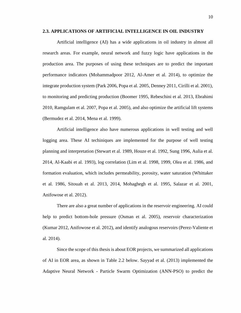
2.3. APPLICATIONS OF ARTIFICIAL INTELLIGENCE IN OIL INDUSTRY

Artificial intelligence (AI) has a wide applications in oil industry in almost all

research areas. For example, neural network and fuzzy logic have applications in the

production area. The purposes of using these techniques are to predict the important

performance indicators (Mohammadpoor 2012, Al-Amer et al. 2014), to optimize the

integrate production system (Park 2006, Popa et al. 2005, Denney 2011, Cirilli et al. 2001),

to monitoring and predicting production (Boomer 1995, Rebeschini et al. 2013, Ebrahimi

2010, Ramgulam et al. 2007, Popa et al. 2005), and also optimize the artificial lift systems

(Bermudez et al. 2014, Mena et al. 1999).

Artificial intelligence also have numerous applications in well testing and well

logging area. These AI techiniques are implemented for the purpose of well testing

planning and interpretation (Stewart et al. 1989, Houze et al. 1992, Sung 1996, Aulia et al.

2014, Al-Kaabi et al. 1993), log correlation (Lim et al. 1998, 1999, Olea et al. 1986, and

formation evaluation, which includes permeability, porosity, water saturation (Whittaker

et al. 1986, Sitouah et al. 2013, 2014, Mohaghegh et al. 1995, Salazar et al. 2001,

Anifowose et al. 2012).

There are also a great number of applications in the reservoir engineering. AI could

help to predict bottom-hole pressure (Osman et al. 2005), reservoir characterization

(Kumar 2012, Anifowose et al. 2012), and identify analogous reservoirs (Perez-Valiente et

al. 2014).

Since the scope of this thesis is about EOR projects, we summarized all applications

of AI in EOR area, as shown in Table 2.2 below. Sayyad et al. (2013) implemented the

Adaptive Neural Network - Particle Swarm Optimization (ANN-PSO) to predict the

11

Minimal Miscible Pressure (MMP) for CO2 flooding projects by using 9 reservoir

parameters, which are reservoir temperatures, mole percentage of oil components,

molecular weights of the heavy fraction (C5+), and mole percentage of the non- CO2

components (Cl, N2, H2S, and C2-C4) in the injected gas. Alikhani (2011) uses Adaptive

Neuro Fuzzy Inference System (ANFIS) to predict the ultimate oil recovery for microbial

method by using porosity, permeability, salinity, temperature, pressure, and pH. Siena

(2015), Alvarado (2002), and Babushkina (2013) all use the same physical reservoir

parameters (porosity, permeability, depth, temperature, gravity, viscosity) in the whole

EOR data set, but the purpose of using clustering algorithm are different. In Siena’s paper,

Bayesian Hierarchical Clustering Algorithm was implemented to predict EOR methods for

unknown EOR projects and the Principal Component Analysis (PCA) was used for the

purpose of data visualization. Alvarado used the machine learning for the same intention

to predict EOR methods, but he used a 2D map to present his results. Moreover,

Babushkina uses K-means and Hierarchical Agglomerative Clustering Algorithm to

predict the oil recovery.

Table 2.2. Artificial intelligence applications in EOR research area

Publications EOR

Methods Applications

Artificial

Intelligence

Algorithms

Input Parameters

Sayyad, H.,

et al. (2013)

CO2

flooding Predict MMP ANN-PSO

Reservoir Temperature,

Mole Percentage of Oil

Components, Molecular

Weights of the Heavy

Fraction (C5+), Mole

Percentage of the Non-

CO2 components (Cl, N2,

H2S, and C2-C4) in the

injected gas

12

Table 2.2. Artificial intelligence applications in EOR research area (cont.)

Alikhani, P.,

et al. (2011)

Microbi

al

Predict Oil

Recovery

Adaptive

Neuro

Fuzzy

Inference

System

(ANFIS)

Porosity, Permeability,

Salinity, Temperature,

Pressure, pH

Siena, M., et

al. (2015)

All

EOR

Forecasting

EOR potential

Bayesian

Hierarchical

Clustering

Algorithm


Depth, Temperature,

Gravity, Viscosity

Alvarado,

V., et at.

(2002)

All

EOR

Predict EOR

Methods

Machine

Learning


Depth, Temperature,

Gravity, Viscosity

Babushkina,

E. V. (2013)

All

EOR

Multi-

dimensional

interpolation

of recovery

factor

K-means

and

Hierarchical

Agglomerati

ve

Clustering

Algorithm


Depth, Temperature,

Gravity, Viscosity

13

3. DATA PRE-PROCESSING

As mentioned in literature review section, the agglomerative hierarchical clustering

algorithm has been implemented for both steam flooding projects and the whole EOR data

set collected from the biannually EOR survey from the Oil and Gas Journal. Before

implementing clustering algorithms into these data set, data preprocessing procedures need

to be taken for duplicate elimination, missing data prediction and senseless data erasing.

With refined data, analysis can be operated in order to decide how the data can be used.

3.1. RAW DATA

The steam flooding data set is collected from 1980 to 2012 Biannually EOR Survey

from the Oil and Gas Journal. Eight reservoir parameters were selected for data analysis,

including one categorical feature and seven numerical features. The categorical feature is

the formation type, and the numerical feature are porosity, permeability, depth, viscosity,

API gravity, temperature, and oil saturation before steam flooding, as shown in Table 3.1.

The reason for selecting these properties to build up our data set is because they are the

main reservoir properties that could describe reservoirs, and these properties are commonly

used for EOR projects data analysis.

Table 3.1. Features of steam flooding projects

Properties Features

Formation Type Categorical

Porosity Numerical

Permeability Numerical

Depth Numerical

API Gravity Numerical

Viscosity Numerical

Temperature Numerical

Oil Saturation, start Numerical

14

For the whole EOR projects, all the data were collected from the biannually EOR

survey from the Oil and Gas Journal from 1998 to 2012. Eighteen reservoir parameters

were utilized for data preparation, including two categorical features and sixteen numerical

features, as shown in Table 3.2. The two categorical features are the EOR methods and

formation type. Besides all the numerical features used in steam flooding projects, the

whole EOR projects add one extra feature into selection, which is the oil saturation after

the utilization of EOR techniques, and each numerical features have both minimum and

maximum values.

Table 3.2. Features of whole EOR projects

Properties Features

EOR Methods Categorical

Formation Type Categorical

Porosity (min, max) Numerical

Permeability (min, max) Numerical

Depth (min, max) Numerical

API Gravity (min, max) Numerical

Viscosity (min, max) Numerical

Temperature (min, max) Numerical

Oil Saturation, start (min, max) Numerical

Oil Saturation, end (min, max) Numerical

3.2. DATA QUALITY CONTROL METHODS

Data quality is important for data analysis. Having the most comprehensive and up

to date information could help to ensure that the analyzing result is correct and useful. For

the established data sets, three problems were concerned: duplicate data, missing data, and

15

senseless data. For both data sets, we applied the same methods to improve the quality of

the data sets.

3.2.1. Duplicate Data. Duplicate data were the first problem that been concerned

during data pre-processing process. Two types of duplicate data were observed. One is the

data that is exactly the, another is the data that has slightly different records among the

projects. Before analyze the data sets, this problem has to be solved to avoid the redundancy

of information, and the biased results. For example, for the worldwide EOR data set, the

data collected includes various EOR methods, like steam flooding, polymer flooding, CO2

miscible flooding, if the data sets have duplicate projects, the percentage of the number of

each EOR method will be incorrect. Moreover, in the EOR data prediction part, the success

percentage of each EOR method in each cluster will be inaccurate (e.g. change the success

percentage of steam flooding from 20% to 50%), which not only leads to the wrong results,

but also may change the results of decision making among the selection of EOR methods

for unknown projects.

To avoid the problems caused by the duplicate data, a series actions has been

conducted, as shown in Figure 3.1. Firstly, the duplicate projects were deleted if projects

are with the exact same records. Then for the data with little different records, two different

cases were under consideration. If the difference is caused by the missing values in the

project and the other values remain the same, project with missing values were deleted. If

projects that have just one feature different, the comparison of irrelevant information

between projects were conducted (like report year, project locations). If the irrelevant

information are the same, the projects were considered as repeating projects; if they have

different irrelevant information, the reservoir properties and fluid properties might

16

coincidentally be the same. Therefore, projects with different irrelevant information were

kept in the data sets.

Figure 3.1. Decision processes with duplicate data

3.2.2. Missing Data. Missing data is a common problem in a data set. Since the

hierarchical clustering algorithm and the principal component analysis algorithm cannot

analyze the projects with missing values, projects with missing values should either to be

imputed or delete the whole projects with missing values. Both methods have pros and

cons. For imputation, it could help to keep as many projects as possible, but may lead to

the biased results (single imputation). However, if the projects with missing data are

ignored or deleted, even though data within the data set are real and not biased, it may

shorten the size of the data set dramatically. Therefore, choosing appropriate methods

dealing with missing data is not an easy decision to make, and it needs a lot of future studies.

In this research, to dealing with this problem, single imputation (mode) were

utilized for numerical data, and projects were deleted if any selected categorical feature(s)

is not available.

Exact same Delete

Slightly different

Missing value Delete

One different value

Irrelevant information

sameDelete

Irrelevant information

differentKeep

17

3.2.3. Senseless and Inconsistent Data. Data which is abnormal or does not make

sense were considered as a sort of senseless. For example, it is impossible to have an EOR

projects under the condition of 0 °F, or with 0 °API. In this case, all zeros in the data sets

are treated as missing data, and they were processed as the methods used for missing values.

Inconsistent data is another problem that have been found in the data sets. For the

categorical features, like the formation type, the combination of dolomite and tripolitic

chert were recorded into several format; for the numerical features, especially for

saturations, some of the value were recorded decimals (0.3), and some of them are in

percentage (30%). To improve the quality of data sets, all data were changed into a certain

format to keep the consistence.

3.3. CLEANED DATA SETS AND STATISTICS

After pre-processed the steam flooding projects, 409 projects were retained, and the

formation type distributions are illustrated in Figure 3.2. Sandstone and unconsolidated

sand are the most common types for steam flooding projects, which sandstone occupies

88% among all the projects, and unconsolidated sandstone formation type takes 10%.

Figure 3.2. Pie chart of formation type distributions for steam flooding projects (from

1980 to 2012 Oil and Gas Journal)

Sandstone, 361, 88%

Unconsolidated

Sand, 40, 10%

Sandstone+Conglo…

Limestone, 2, 1%

Sandstone+Dolomite, 1, 0%

Dolomite, 1, 0%Fractured Chert-

Dolomite, 1, 0%

Conglomerate, …Other, 8, 2%

18

For worldwide EOR projects data set, after the data pre-processing process, 726

EOR projects remained in total, which includes thirteen different EOR methods (Steam

flooding, CO2 miscible flooding, CO2 immiscible flooding, hydrocarbon miscible flooding,

hydrocarbon immiscible flooding, polymer flooding, nitrogen miscible flooding, nitrogen

immiscible flooding, microbial, hot water, surfactant flooding, chemical flooding, and

combustion.) and seven formation types (sandstone, dolomite, limestone, tripolitic,

unconsolidated sandstone, shale, and conglomerate). Figure 3.3 and Figure 3.4 present the

distribution of different EOR projects and the distribution of formation types.

Figure 3.3. Project distributions of EOR methods (from 1996 to 2012 Oil and Gas

Journal)

As illustrated in Figure 3.3, CO2 miscible flooding and steam flooding are the two most

popular EOR methods, which has 325 projects and 237 projects, respectively, and occupies

75 % of the overall EOR projects in total. For the formation type which shown in Figure

3.4, in contrast with the steam flooding projects, the overall EOR projects are mainly with

CO2 Miscible,

325, 43%

Steam, 237, 32%

Hydrocarbon

Miscible, 53, 7%

Polymer, 33, 4%Combustion, 25, …

Chemical, 21, 3%

CO2 Immiscible, …Nitrogen

Immiscible, 12,

2%

Hot Water, 7, 1%

Surfactant, 6, 1%

Hydrocarbon

Immiscible, 4,

1%

Nitrogen Miscible, 3,

0%

Microbial, 3, 0%Other, 23, 3%

19

the formation type of sandstone and carbonate (dolomite and limestone), which takes 49%

and 37% of all the projects, respectively, and not many projects with shale, conglomerate,

unconsolidated sand formation type EOR projects were reported in the Oil and Gas Journal

EOR Survey.

Figure 3.4. Project distributions of formation type for worldwide EOR projects (from


Sandstone, 418,

49%

Dolomite, 221,

26%

Limestone, 91, 11%

Tripolitic, 44, 5%

Unconsolidated

Sand, 42, 5%

Shale, 18, 2%

Conglomerate,

18, 2%Other, 78, 9%

20

4. DATA ANALYSIS METHODS

After data preparation, hierarchical clustering analysis, descriptive statistics, and

principal component analysis were utilized to reveal the hidden relationships among

projects; to characterize the clusters; and to visualize the results and to figuring out the

governing features in the data sets.

Figure 4.1 is the workflow of data analysis process. Hierarchical clustering

algorithms were implemented to study the hidden knowledge in the data sets. The results

of this process are dendrograms and clusters which could show the distances and grouping

results among projects. Within a cluster, projects are similar with each other, which share

the similar characteristics.

Figure 4.1. Workflow of data analysis process

In order to reveal the characteristics of each cluster, descriptive statistics approach

comes to the stage for data analysis. Correlation coefficient are used to study the

relationships among reservoir properties; statistical graphics, like box plots and bar charts

are generated to know the property ranges; and descriptive statistical summaries are used

to show the statistical results.

Last but not least, principal component algorithms are also implemented in the

clustering results to visualize the results and filter out the dominating reservoir properties

Implementation of Hierarchical Clustering

Descriptive Statistics

Principal Component Analysis

21

in the data sets. Mono plots are generated to not only indicates the relationships of reservoir

properties, but also presents the most import factors in the data sets; scatter plots are used

to show the relationship of projects in a 2D map. The following subsections briefly describe

these computational and visualization techniques.

4.1. HIERARCHICAL CLUSTERING ANALYSIS

Hierarchical clustering is a method of cluster analysis in data mining, which groups

data with a sequence of nested partitions, either from singleton clusters to a cluster

including all individuals or vice versa (Xu, Wunsch, 2010). This method is generally

divided into two types: agglomerative hierarchical clustering and divisive hierarchical

clustering. Figure 4.2 below illustrates the difference between these two clustering.

Agglomerative hierarchical clustering is a ‘bottom up’ method where each observation

represents as an individual cluster at the beginning, two clusters are then merged in each

step until all objects are forced into the same group. Divisive hierarchical clustering is a

‘top down’ method where all observations start in one cluster, and splits are performed

recursively as one moves down the hierarchy (Reference 16). For this research, the

agglomerative hierarchical clustering was used.

Agglomerative

Hierarchical

Clustering

Divisive

Hierarchical

Clustering

Figure 4.2. Hierarchical clustering

22

Agglomerative clustering starts with N clusters, each of which includes exactly one

data point. The conduction of merge operation is determined by the computation of

distance, which represents the similarities and dissimilarities among clusters. If the distance

between two clusters is the shortest, they will merge into a bigger cluster.

In other words, data points within the same cluster are similar to one another, and

dissimilar to the data points in other clusters. The greater the similarity or homogeneity

within a group and the greater the difference between groups is, the better or more distinct

the clusters are. The general agglomerative clustering can be summarized by the following

procedure, which is also summarized in Figure 4.3.

There are three main reasons why the clustering algorithm was implemented in the

oil industry. First, data set are typically multi-dimensional, it is difficult to know their

similarities or relationships. Secondly, by utilizing the clustering algorithm, it is easy to

characterize the data after clusters are formed, which means the hidden knowledge and

characteristics could be revealed. Last but not least, cluster results provide more

information about the data set compared with the ranges, and this makes the results more

accurate and reliable.

As mentioned previously, distance is important because it determines how clusters

merged each other. In this research, the Manhattan Distance for numerical features dues to

this method is commonly used, which is defined as:

d(p, q) = |a1x1 − a1x2|+|a2x1 − a2x2|+|a3x1 − a3x2|+…+|anx1 − anx2|

and the distance for categorical feature between p and q is:

𝑑(𝑝, 𝑞) = {10

𝑖𝑓 𝐴𝑁𝐷(𝑝, 𝑞) = 0

𝑜𝑡ℎ𝑒𝑟𝑤𝑖𝑠𝑒

23

After the computation of the Manhattan Distances the distance of each numerical

feature was normalized from 0 to 1 to pair with the distance calculated in categorical

features, and to ensure that all the features are equally weighted. Moreover, the weighted

average linkage was utilized to define the distance function between two clusters.

Another important task is the determination of clustering levels. In this research,

the clustering output for both steam flooding and EOR data sets stops at clustering level 20

with dendrograms. With these dendrograms, cluster stability analysis is studied to filter out

Start

Represent each point

as a cluster

Calculate the

proximity matrix

Merge a pair of clusters with

the minimal distance

One cluster

left?

Generate the clusters by cutting the

dendrogram at an appropriate level

Yes

End

No

Figure 4.3. Flowchart of the agglomerative hierarchical clustering algorithm. (Rui

Xu and Donald C. Wunsch II, 2010) [Reference 17]

24

the outliers and the main clusters. Therefore, by analyzing the stability of clusters,

clustering level could be determined.

4.2. DESCRIPTIVE STATISTICS

When analyzing reservoir parameters, scatter plots in correlation coefficients can

quickly uncover patterns, and reduce large amount of data to a subset of interesting

relationships. Correlation describes the strength the relationship between two variables,

correlation coefficient ranges from -1 to 1. 1 indicates a perfect positive linear relationship

and -1 in the case indicates perfect negative linear relationship. 0 indicates that variables

are uncorrelated, and there is no linear relationship. Normally, the correlation coefficient

lies between these values.

Figure 4.4 below illustrates the concepts. The top two rows present the linear

relationships between two variables, and the bottom row indicates the non-linear

relationships, which are in different shapes.

Figure 4.4. Correlation coefficient [Reference 50]

25

In this research, the Pearson’s Correlation Coefficient has been used to measure the

strength of the association between the two properties. The modified effects of different

Pearson’s Correlation Coefficients (𝑟) are shown in Figure 4.5 (Reference 57). For 𝑟 falls

into the range of -0.3 to +0.3, it means the two properties are not very related to each other;

for r from ±0.3 to ±0.5, it shows that the properties are relatively related; and for r equal or

greater than ±0.5, it indicates that the two properties are strongly related.

Figure 4.5. Effects of different Pearson's Correlation Coefficients [modified, Reference

57]

4.3. PRINCIPAL COMPONENT ANALYSIS

In this research, Principal Component Analysis (PCA) were implemented for the

following purposes: 1) to figure out the dominating factors (reservoir parameters) in the

data set; and 2) to present the clustering result in a 2D map, which helps to understand the

relationships between clusters and the EOR projects.

4.3.1. Principal Component Analysis. In order to understand the theory behind

the PCA method, a simple example is given and shown in Figure 4.6a. For a two-

dimensional (2D) data set, if one dimensional is the goal to achieve, in another word, reduce

from two dimensional to one dimensional, a projection line will be needed to represent the

26

data (as the red line shown in Figure 4.6b). If the original data were projected onto a red

line, green points could be get as shown in Figure 4.6c, and the distance between each point

and the projected version is pretty small. Figure 4.6d displays the lower dimensional (1D)

results after the dimensionality reduction. The projection line could represents the locations

of the each data point with the minimized variance reduction in the original data set.

Figure 4.6. Dimensionality reduction example

Therefore, the PCA method finds a lower dimensional surface (from 2D to 1D in

this case) to project the data. In other words, PCA is a method that find the minimized sum

27

of squares of distance between original data and the projected points. The distance between

original data and the projected point is called the projection error. In a general case, for a

𝑛 dimensional data set, any dimensions (𝑘) could be achieve by implementing PCA if

n>k>2.

4.3.2. Principal Component Analysis Procedures. In this subsection, the

procedures for PCA is presented to help better understand the how to use PCA for a real

project, especially for the steam flooding and worldwide EOR projects, which includes

data pre-processing, implementation, choosing the number of principal components, and

the visualization with mono plot.

Step 1. Data Pre-processing for PCA. It is always important to perform mean

normalization, and then depending on the data, maybe perform feature scaling as well. Data

should be prepared without missing data, duplicate data, and inconsistent data as mentioned

in section 3.

Step 2. Implementation of PCA. After finishing data pre-processing, PCA were

implemented. Take Figure 4.6 as an example (from 2D to 1D), there are mainly two things

what PCA does. The first one is PCA helps to find the projection line (red line), the second

thing is it helps to compute the numbers or the locations of the projection data on the red

line. In another case, if a two dimensional data is the goal to achieve from a three

dimensional data set, what PCA does is it firstly find the 2D plane with the minimum sum

square of distance between the original data and the projection plane, then it needs to

calculate the location of projection points in the 2D plane.

Step 3. Choosing the number of principal components. For a 𝑛 dimensional data

set, a 𝑛 principal components will be got, which contains the 100% of the information of

28

the original data. However, to reduce the dimensions, not all principal components need to

be utilized. Usually, a PCA algorithm should retain about 90% of the variance for a good

result after dimensionality reduction, therefore, the number of principal components could

be determined.

In this research, the agglomerative hierarchical clustering algorithm was

implemented for both the steam flooding projects and the whole EOR data set. Seven

important reservoir parameters were selected for steam flooding projects, and sixteen

variables for the whole EOR data set. So multi-dimensional data sets (seven dimensional

and sixteen dimensional) need to be presented in a two dimensional or three dimensional

in order to visualize and better present our data. Meanwhile, 90% of the variance should

be retained.

Step 4. Visualization using mono plot. A two dimensional correlation mono plot of

the first two principal components can visualize the relationships between variables, as

shown in Figure 4.7. The correlation mono plot shows vectors pointing away from the

origin to represent the original variables. The angle between two vectors is an

approximation of the correlation between the variables. A small angle indicates the

variables are positively correlated, and angle of 90 degrees indicates the variables are not

correlated, and an angle close to 180 degrees indicates the variables are negatively

correlated. The length for the line and how it closes to the circle indicates how well the

variable is represented in the plot.

29

Figure 4.7. Mono plot explanations

30

5. RESULTS FROM STEAM FLOODING DATA SET

In this section, the results of the hierarchical clustering analysis, descriptive

statistics, and the principal component analysis are displayed for the steam flooding

projects.

5.1. HIERARCHICAL CLUSTERING RESULTS

After the implementation of hierarchical clustering algorithm, 20 clusters were

achieved. Figure 5.1 is the compact visualization of the results, and Figure 5.2 indicates

the detailed clustering results of clustering level 20.

Figure 5.1. Steam flooding clustering results (from 1980 to 2012 Oil and Gas Journal)

The horizontal axis in Figure 5.1 represents clusters, and the vertical axis indicates

the distance between clusters. With the process of clusters merge, the distance between

clusters are greater, which means clusters are more dissimilar.

269279276383387337 1253353386385 76156157361355371 7 15153255 82138 87136185 11 16 20 49360370372349 93356363362366167231232244297236180352240305357368374373382358364365359369376381377378379375380384345351354 9 10 21 22324325326 23330323341342347348 17 18 95115104106105117119118120 94238 38 39190319 81133134186184209212211280287 80 84 91 92150160169152161162163168165166235237243207218271277213288254283289286292293294295220224225226229222234298301296124126164291147284290233239299300303304149154221230208241307247 79116 88 90 89204155158159228100101108242256258257302 85 86110 99320331103107125327328332339321334335336333 25 26137 27148227135217195196201223268272281275270316273315317314 45 51 46 47 48200188191122182130 73318388389260 77112113114139142143197202203205179282193194267140145141189199146216285151210144206219274278123183187131259178 58306 2 3 4 5 6 8198 78 83111102127170 74 75 40129264 28 30 31 29 32 33 37 34 35 36 41 50 52 53 56 57 60 61 63 55 62 59 64 65 66329 69 70 67 68 72 71132262265263266322338340 97 98192215214245246 12 13 19 96173174109121176177308310311309 14 24249250367 54171172343346350344175248 42 43 441812522512613123131280

0.5

1

1.5

2

2.5

31

Figure 5.2. Hierarchical clustering results using hierarchical level of 20

32

As seen from the dendrogram in Figure 5.2, the hierarchy structure of all the steam

flooding data is clearly laid out. Each element in the dendrogram represents the hierarchical

clustering result at each clustering level. In this dendrogram, S stands for sandstone

formation, D represents dolomite formation, U indicates the unconsolidated sandstone

formation, C is the conglomerate formation, and L is the limestone formation. Figure 5.3

is the expressions of one cluster from cluster level 9. C1 (301S+1D+1C) represents the

name of this cluster is called cluster 1, and it is the biggest cluster in this level. This cluster

includes 301 records with sandstone formation type, 1 record of dolomite formation, and 1

record of conglomerate formation.

Figure 5.3. Expression of the Cluster 1 in cluster level 9

Since the agglomerative hierarchical clustering algorithm were used as indicated

before, this dendrogram is a bottom-up structure, which starts at the bottom of the

dendrogram and treat each project as an individual cluster. Clusters are merged each other

into a bigger cluster at each clustering level by compute and compare the distances until

all the projects were formed into the same cluster. In other words, clusters with similar

characteristics are tend to merge earlier in the dendrogram, vice versa.

33

As illustrated in the dendrogram, all the elements are well distributed based on the

formation type. Moreover, on the right side of the dendrogram, cluster 17 and cluster 19

formed a quite stabled cluster during the hierarchical clustering process. In this case, cluster

17 and cluster 19 represents were considered as outliers in the data set because they are

dissimilar with other clusters so that they are not able to merge with other clusters.

In order to get better understanding of each specific cluster and to study the

characteristics for each cluster, the domain knowledge of steam flooding and range for each

properties are applied as shown in Table 5.1 based on the study of steam flooding projects

data set and the common knowledge for steam flooding.

Table 5.1. Domain knowledge for steam flooding

Property Category Average value range

Oil viscosity (cp)

High ≥5000

Medium [1000, 5000]

Low <1000

Formation porosity (%) High [25,50]

Low <25

Formation permeability (md)

High ≥ 5000

Intermediate high [1000, 5000]

Intermediate low [100, 1000]

Low <100

Formation depth (ft)

Deep ≥ 3000

Intermediate deep [1000, 3000]

Intermediate shallow [500, 1000]

shallow <500

34

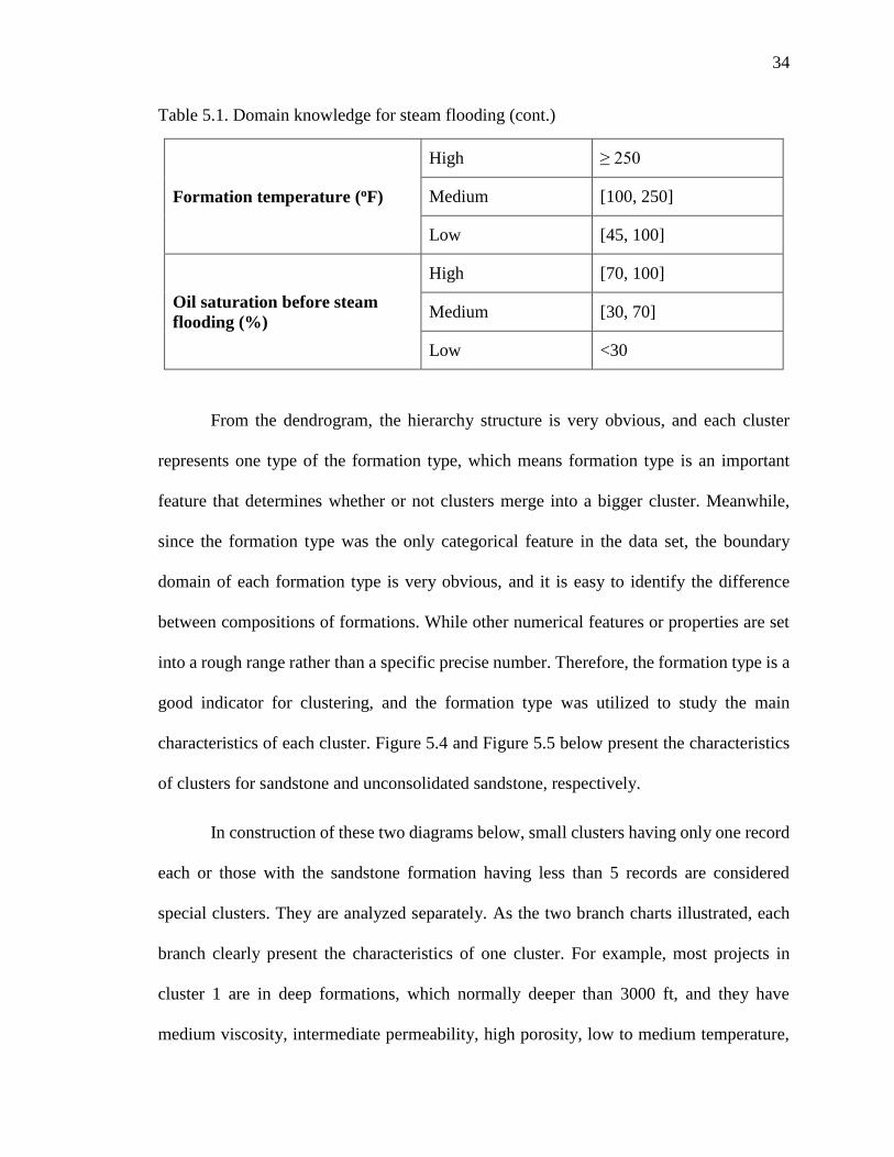
Table 5.1. Domain knowledge for steam flooding (cont.)

Formation temperature (oF)

High ≥ 250

Medium [100, 250]

Low [45, 100]

Oil saturation before steam

flooding (%)

High [70, 100]

Medium [30, 70]

Low <30

From the dendrogram, the hierarchy structure is very obvious, and each cluster

represents one type of the formation type, which means formation type is an important

feature that determines whether or not clusters merge into a bigger cluster. Meanwhile,

since the formation type was the only categorical feature in the data set, the boundary

domain of each formation type is very obvious, and it is easy to identify the difference

between compositions of formations. While other numerical features or properties are set

into a rough range rather than a specific precise number. Therefore, the formation type is a

good indicator for clustering, and the formation type was utilized to study the main

characteristics of each cluster. Figure 5.4 and Figure 5.5 below present the characteristics

of clusters for sandstone and unconsolidated sandstone, respectively.

In construction of these two diagrams below, small clusters having only one record

each or those with the sandstone formation having less than 5 records are considered

special clusters. They are analyzed separately. As the two branch charts illustrated, each

branch clearly present the characteristics of one cluster. For example, most projects in

cluster 1 are in deep formations, which normally deeper than 3000 ft, and they have

medium viscosity, intermediate permeability, high porosity, low to medium temperature,

35

and medium to high oil saturation. In other words, the branch of cluster 1 represents the

common reservoir property ranges similarly like the conventional screening methods.

However, the other branches also explains different suitable cluster ranges under different

reservoir conditions.

Figure 5.4. Cluster characterization of steam flooding applications on sandstone formations.

The red colored clusters have less dominating value ranges so that all the detailed

categories are presented; the black colored clusters have dominating categories in

respective properties

36

Figure 5.5. Cluster characterization of steam flooding applications on unconsolidated sands

formations. The red colored clusters have less dominating value ranges so that all the

detailed categories are presented; the black colored clusters have dominating categories in

respective properties.

Moreover, steam flooding has a wide application with different reservoir conditions.

For sandstone formations, the formation depth varies significantly, from 100 feet to 9000

feet; each depth category reveals different associations among selected properties. For

example, deep formation applications correspond to viscous oils, high porosity and

intermediate high permeability, initial oil saturation greater than 70%, but there are

significant number of applications fall into low temperature range of 45 ~ 100 ˚F; yet

37

shallow formation applications correspond to the same high porosity but lower

permeability formations, lower viscous oils and lower formation temperatures.

Comparing with a simple screening table presents in conventional screening

methods, by having these two branch charts, more detailed screening information are

displayed. Moreover, for a new project, if the formation type is unconsolidated sandstone,

and the depth is intermediate deep, the viscosity falls into the range of low, and has high

permeability and high porosity, the ranges of temperature and oil saturation could be

achieved.


After the clustering results, descriptive statistics methods were utilized to

understanding the relationship between reservoir parameters.

5.2.1. Correlation Coefficient. Tables of 5.2 and 5.3 indicate the Pearson’s

Correlation Coefficient between paired properties for the two biggest clusters (cluster 1

and cluster 2), respectively. From cluster 1, the biggest correlation coefficient is between

the viscosity and API, which is -0.33; and the least related features are viscosity and

permeability. In cluster 2, the strongest relationship is between API and temperature, which

is -0.47, and the least related properties are temperature and permeability.

Table 5.2. Pearson’s Correlation Coefficients between paired properties for cluster 1

Porosit

y %

Permeabilit

y, md

Dept

h, ft

AP

I

Viscosit

y, cp

Temperatur

e, F

Residual

oil

Saturatio

n. Start

Porosity % 1

Permeabilit

y, md 0.06 1

Depth, ft -0.30 0.08 1

38


(cont.)

API 0.05 0.18 -0.05 1

Viscosity, cp -0.20 0.00 0.03 -

0.33 1

Temperature

, F 0.07 0.10 0.16

-

0.19 -0.27 1

Residual oil

Saturation.

Start

-0.07 0.12 -0.08 -

0.16 0.14 0.07 1


Porosi

ty %

Permeabili

ty, md

Dept

h, ft

AP

I

Viscosit

y, cp

Temperatu

re, F

Residual

oil

Saturatio

n. Start

Porosity % 1

Permeabilit

y, md -0.29 1

Depth, ft -0.30 0.28 1

API -0.09 -0.39 -0.21 1

Viscosity,

cp 0.06 0.20 -0.22

-

0.3

2

1

Temperatu

re, F 0.31 0.01 0.27

-

0.4

7

-0.11 1

Residual oil

Saturation.

Start

-0.06 -0.16 -0.36

-

0.1

6

0.23 -0.21 1

Even though the relationship associations are different in some of the paired

properties, for example, in cluster 1, porosity is positively associated with permeability,

which is 0.06; while it is negatively associated in cluster 2, which is -0.29, the most of the

paired properties have a consistent relationships. For instance, the relationship between

API and temperature is always negatively associated, which means with the increase of

39

temperature, the API drops down. Similarly, saturation vs. porosity, depth, and API; API

vs. depth, viscosity, and temperature; and temperature vs. viscosity are all negatively

correlated. On the other hand, permeability vs. depth and temperature; temperature vs.

porosity and depth; and saturation vs. viscosity are positively associated.

5.2.2. Box Plots. To better understanding the characteristics of each clusters,

boxplot and bar charts have been used to represents the ranges of each cluster and the

distribution of properties for each cluster. These two sets of plots are generated for both

sandstone formations and unconsolidated sand formations.

Figures 5.6 to 5.12 present the boxplots of each reservoir parameter, which are

porosity, permeability, depth, API gravity, temperature, viscosity and oil saturation at start.

Figure 5.6. Porosity ranges in boxplot for steam flooding projects (from 1980 to 2012 Oil

and Gas Journal)

15 20 25 30 35 40 45

Cluster 1Cluster 2Cluster 3Cluster 5Cluster 6

Cluster 8Cluster 9

Cluster 10Cluster 4Cluster 7

Cluster 12Cluster 15Sandstone

UnconsolidatedOverall

Porosity, %

40

From this plot, the overall ranges of porosity for steam flooding projects is from 18

to 40.5. The difference between sandstone formation and unconsolidated sandstone

formation is not obvious. However, unconsolidated sandstone formation tends to have

relatively biased porosity. For example, cluster 7 mainly includes the steam flooding

projects with high porosity, while main projects in cluster 12 has low porosity. For both

formation type, most projects falls into the porosity ranges from 30 to 35.

Figure 5.7. Permeability ranges in boxplot steam flooding projects (from 1980 to 2012

Oil and Gas Journal)

Figure 5.7 above presents the ranges of permeability for steam flooding projects.

The overall ranges of permeability is from 11mD to about 20000 mD, and most of the

projects have the permeability from 1000 mD to 3000 mD. For the sandstone formation

type, the permeability of cluster 3 seems to have large distance with other clusters because

1 10 100 1000 10000 100000

Cluster 1

Cluster 2

Cluster 3

Cluster 5

Cluster 6

Cluster 8

Cluster 9

Cluster 10

Cluster 4

Cluster 7

Cluster 12

Cluster 15

Sandstone

Unconsolidated

Overall

Permeability, mD

41

this cluster involves the majority of the projects with low permeability. Cluster 10 tends to

include the projects with high permeability. For the unconsolidated formation type, the

ranges of permeability is relatively more concentrated because there are less steam flooding

projects with this formation type compared with sandstone formations. As we could see in

the plot, most projects in cluster 7 has almost the same permeability values, which is about

1500 mD.

Figure 5.8. Depth ranges in boxplot steam flooding projects (from 1980 to 2012 Oil and

Gas Journal)

Figure 5.8 shows the ranges of depth for steam flooding projects. The overall

projects have a huge ranges from extremely shallow reservoirs (about 100 ft) to very deep

reservoirs (about 9200 ft). Based on the ranges of each cluster, we could find that some of

the clusters are very unique, and some of the clusters have similar ranges. For example,

0 2000 4000 6000 8000 10000

Cluster 1

Cluster 2

Cluster 3

Cluster 5

Cluster 6

Cluster 8

Cluster 9

Cluster 10

Cluster 4

Cluster 7

Cluster 12

Cluster 15

Sandstone

Unconsolidated

Overall

Depth, ft

42

cluster 6 and cluster 7 are very special in terms of depth among all clusters, both of them

includes the projects with extremely shallow reservoirs. Cluster 1, 2, and cluster 3 have

similar ranges of depth, which means the distance of depths for these three clusters are very

small.

Figure 5.9. Gravity ranges in boxplot for steam flooding projects (from 1980 to 2012 Oil

and Gas Journal)

Figure 5.9 illustrates the ranges of API gravity for all clusters, which is from 7 ̊ API

to 25 ˚API. This ranges indicates that all the steam flooding projects in this data set are

heavy oil. What’s more, it is very surprising that the main ranges of gravity for both

sandstone formation type and unconsolidated formation type are exactly the same, which

shows that the formation type does not have large influence to the oil gravity.

0 5 10 15 20 25 30

Cluster 1

Cluster 2

Cluster 3

Cluster 5

Cluster 6

Cluster 8

Cluster 9

Cluster 10

Cluster 4

Cluster 7

Cluster 12

Cluster 15

Sandstone

Unconsolidated

Overall

Gravity, ˚API

43

By combing all the above plots together, these boxplots indicate that several

clusters have their own special and concentrated small ranges of gravity, like cluster 8,

cluster 10, cluster 12, and cluster 15. In contrast with the small ranges of permeability,

porosity, and depth, cluster 7 has a very large ranges of API gravity, which indicates that

the gravity in cluster 7 is very different, and this might be the reason why cluster 7 did not

merge with other clusters. Moreover, cluster 10 is very special with the parameter of

gravity as well, which has the highest gravity among all clusters.

Figure 5.10. Temperature ranges in boxplot for steam flooding projects (from 1980 to

2012 Oil and Gas Journal)

Figure 5.10 illustrates the ranges of temperature, which is from 55 ˚F to about 235

˚F. Surprisingly, even though there are way less steam flooding projects with

unconsolidated sandstone formation, the ranges of temperature is bigger than the

0 50 100 150 200 250 300

Cluster 1

Cluster 2

Cluster 3

Cluster 5

Cluster 6

Cluster 8

Cluster 9

Cluster 10

Cluster 4

Cluster 7

Cluster 12

Cluster 15

Sandstone

Unconsolidated

Overall

Temperature, ⁰F

44

temperature for the projects with sandstone formation, which may indicate that the

formation type might be a factor that affect reservoir temperature. In addition, the boxplot

of cluster 10 is just a line, which shows that the temperature in this cluster just have 2

different values. When check back the temperature in the cluster 10, 6 projects

coincidentally have exactly same value of temperature (66 ˚F) even though they have

totally different values for other reservoir parameters. Therefore, temperature might be a

dominating feature for cluster 10.

Figure 5.11. Viscosity ranges in boxplot for steam flooding projects (from 1980 to 2012


Figure 5.11 presents the ranges of viscosity for each cluster. The overall ranges of

viscosity is very huge, from 11cP to 1000000 cP, and most projects falls into the range

1 10 100 1000 10000 100000 1000000

Cluster 1

Cluster 2

Cluster 3

Cluster 5

Cluster 6

Cluster 8

Cluster 9

Cluster 10

Cluster 4

Cluster 7

Cluster 12

Cluster 15

Sandstone

Unconsolidated

Overall

Viscosity, cP

45

from 700 cP to 5000 cP. Cluster 15 in the plot is presented by a single line, which means

all the steam flooding projects in cluster 15 have the same value of viscosity, which is 1500

cP. From the plot, cluster 1 and cluster 2 tends to involve the projects with high viscous

fluids, while cluster 3 and cluster 8 tends to have the low viscous fluids.

Figure 5.12. Residual oil saturation ranges in boxplot for steam flooding projects (from


Figure 5.12 indicates the oil saturation ranges before the implementation of steam

flooding. The overall ranges of oil saturation is from 29 to 100. As shown in this plot, the

main ranges to each cluster is very distinctive. For example, cluster 1 has the main ranges

0 20 40 60 80 100 120

Cluster 1

Cluster 2

Cluster 3

Cluster 5

Cluster 6

Cluster 8

Cluster 9

Cluster 10

Cluster 4

Cluster 7

Cluster 12

Cluster 15

Sandstone

Unconsolidated

Overall

Residual Oil Saturation, Start

46

from 53 to 65; cluster 2 has the main ranges from 84.25 to 95. Also, the saturation of cluster

12 is from 63.75 to 65, and the saturation range for cluster 15 is from 56.25 to 58.75.

5.2.3. Bar Charts. From Figure 5.13 to Figure 5.18, the bar charts are used to

indicate the number of record and distributions for each specific ranges of reservoir

properties.

Figure 5.13. Viscosity project records distributions for steam flooding projects (from


As shown in Figure 5.13 above, the main viscosity ranges of cluster 1 and cluster 2

is from 1000 cP to 3000 cP. The main ranges of cluster 3 and cluster 5 is from 100cP to

1000 cP, and cluster 3 also includes the majority projects with the low viscosity. Moreover,

0 50 100 150 200

C1(195)

C2(75)

C3(32)

C4(23)

C5(20)

C6(13)

C7(9)

C8(8)

C9(7)

C10(7)

C12(4)

C15(2)

Number of Records

Clu

ste

rs

[0,100)

[100,1000)

[1000,3000)

[3000,5000)

[5000,10000)

[10000,infinit)

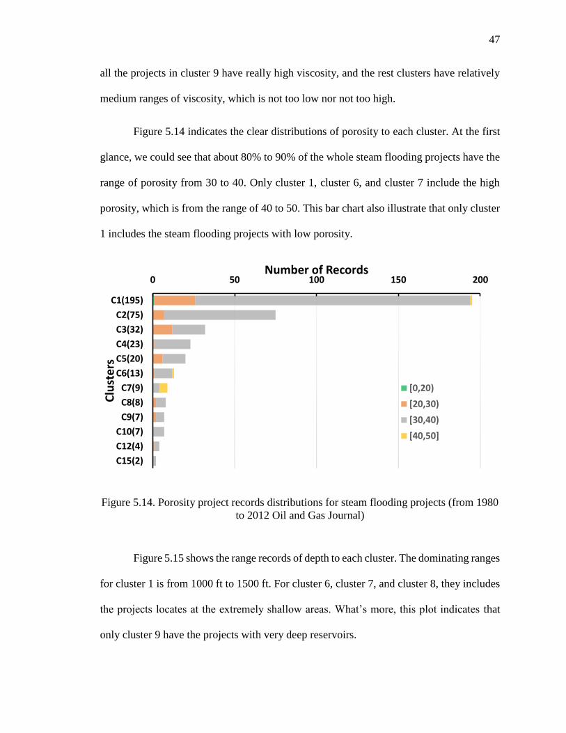
47

all the projects in cluster 9 have really high viscosity, and the rest clusters have relatively

medium ranges of viscosity, which is not too low nor not too high.

Figure 5.14 indicates the clear distributions of porosity to each cluster. At the first

glance, we could see that about 80% to 90% of the whole steam flooding projects have the

range of porosity from 30 to 40. Only cluster 1, cluster 6, and cluster 7 include the high

porosity, which is from the range of 40 to 50. This bar chart also illustrate that only cluster

1 includes the steam flooding projects with low porosity.

Figure 5.14. Porosity project records distributions for steam flooding projects (from 1980

to 2012 Oil and Gas Journal)

Figure 5.15 shows the range records of depth to each cluster. The dominating ranges

for cluster 1 is from 1000 ft to 1500 ft. For cluster 6, cluster 7, and cluster 8, they includes

the projects locates at the extremely shallow areas. What’s more, this plot indicates that

only cluster 9 have the projects with very deep reservoirs.

0 50 100 150 200

C1(195)

C2(75)

C3(32)

C4(23)

C5(20)

C6(13)

C7(9)

C8(8)

C9(7)

C10(7)

C12(4)

C15(2)

Number of Records

Clu

ste

rs

[0,20)

[20,30)

[30,40)

[40,50]

48

Figure 5.15. Depth project records distributions for steam flooding projects (from 1980 to


Figure 5.16. Permeability project distributions for steam flooding projects (from 1980 to


Figure 5.16 shows the records of permeability for different ranges. As we could see,

almost all the clusters have the permeability ranges from 1000 mD to 3000 mD, except

0 50 100 150 200

C1(195)

C2(75)

C3(32)

C4(23)

C5(20)

C6(13)

C7(9)

C8(8)

C9(7)

C10(7)

C12(4)

C15(2)

Number of Records

Clu

ste

rs

[0,500)

[500,1000)

[1000,1500)

[1500,2000)

[2000,3000)

[3000,5000)

[5000,infinit)

0 50 100 150 200

C1(195)C2(75)C3(32)C4(23)C5(20)C6(13)

C7(9)C8(8)C9(7)

C10(7)C12(4)C15(2)

Number of Records

Clu

ste

rs

[0,100)[100,500)[500,1000)[1000,3000)[3000,5000)[5000,infinit)

49

cluster 12. This range also occupies most of the records in cluster 1, and involved the

highest records in cluster 2, 5, 6, 7, 8, and cluster 9 as well. There are several clusters

includes the projects with high permeability, which are cluster 1, 2, 4, 10, and cluster 12.

Figure 5.17 presents the range records of temperature for each cluster. From the

plot, we could see that most clusters have the most records from either 80 ˚F to 100 ˚F, or

from 100 ˚F to 120 ˚F. Cluster 8 and cluster 15 seem to be a little bit different which they

only have the records of extremely high reservoir temperatures, from 180 ˚F to 240 ˚F.

Moreover, cluster 1, 2, and 4 include the all the projects with low temperature, which is

just from 45 ˚F to 60 ˚F.

Figure 5.17. Temperature project records distributions for steam flooding projects (from


Figure 5.18 illustrates the record ranges of oil saturation before the implementation

of steam flooding techniques. Before using steam flooding, we could see that most clusters

already have relatively high oil saturation. For example, the biggest number of records in

0 50 100 150 200

C1(195)

C2(75)

C3(32)

C4(23)

C5(20)

C6(13)

C7(9)

C8(8)

C9(7)

C10(7)

C12(4)

C15(2)

Number of Records

Clu

ste

rs

[45,60)[60,80)[80,100)[100,120)[120,140)[140,160)[160,180)[180,240]

50

cluster 1 has the saturation from 60 to 70 already, which is pretty high. For cluster 2, most

of the projects even have the oil saturation from 80 to 100. Only cluster 1 has the projects

with low oil saturation.

Figure 5.18. Oil saturation project records distributions for steam flooding projects (from


Therefore, each clusters of steam flooding projects could be effectively and clearly

characterized by using hierarchical clustering algorithm. However, several steps still need

to take to get better results:

1. Change the range of each properties, so a smaller range of each cluster could

be achieved.

2. Use other clustering algorithm to process this data set to study which

algorithm works best for steam flooding projects.

5.2.4. Descriptive Statistics Summaries. In order to draw the rules for each cluster,

and to better characterize the clusters for each data set, the descriptive statistics have been

0 50 100 150 200

C1(195)

C2(75)

C3(32)

C4(23)

C5(20)

C6(13)

C7(9)

C8(8)

C9(7)

C10(7)

C12(4)

C15(2)

Number of Records

Clu

ste

rs [0,30)

[30,40)

[40,50)

[50,60)

[60,70)

[70,80)

[80,100)

51

summarized. For steam flooding projects, four new clusters were formed based on the

existing 20 clusters and the dendrogram, as shown in Table 5.4.

Table 5.4. 20 clusters merged into 4 big clusters for steam flooding projects

New Cluster Merged Clusters

Cluster 1 Clusters 1, 2, 6, 9, 10, 11

Cluster 2 Clusters 3, 5, 8, 13

Cluster 3 Clusters 4, 7, 12, 15, 16, 17, 20

Cluster 4 Clusters 14, 18, 19

Figure 5.19 indicates the descriptive statistic summaries for steam flooding clusters.

As shown in the figure, the porosity does not distinct with each other between clusters,

except cluster 4 concludes the steam flooding projects with relatively low porosity (18%).

What’s more, cluster 1 and cluster 3 involve the projects with high permeability and high

viscosity; cluster 2 and cluster 4 have the projects with extremely high temperature; and

cluster 3 includes the projects with rarely deep formations (9000 ft).

15 20 25 30 35 40 45

Cluster 1

Cluster 2

Cluster 3

Cluster 4

Porosity, %

Figure 5.19. Properties summaries for steam flooding (from 1980 to 2012 Oil and Gas

Journal)

52

1 10 100 1000 10000 100000

Cluster 1

Cluster 2

Cluster 3

Cluster 4

Permeability, md

0 2000 4000 6000 8000 10000

Cluster 1

Cluster 2

Cluster 3

Cluster 4

Depth, ft

0 5 10 15 20 25 30

Cluster 1

Cluster 2

Cluster 3

Cluster 4

Gravity, ˚API

10 100 1000 10000 100000 1000000

Cluster 1

Cluster 2

Cluster 3

Cluster 4

Viscosity, cp


Journal) (cont.)

53


Journal) (cont.)


Figure 5.20 is a mono plot for steam flooding projects. the length of the viscosity

vector is the largest, and is closest to the circle, this results represents that viscosity is the

most important reservoir parameters in the steam flooding projects. Moreover, depth and

permeability are also long vectors in the mono plot, therefore, these two reservoir

parameters are also very important in the steam flooding projects compared with other

parameters (temperature, oil saturation, gravity, and porosity). On the other hand, the mono

plot also illustrates that permeability and depth are almost not correlated, and viscosity is

negatively correlated with permeability and depth, respectively.

By comparing the results from the study of correlation coefficient and the mono

plot, the mono plot is a better way to figure out the relationships among reservoir properties,

0 50 100 150 200 250 300

Cluster 1Cluster 2Cluster 3Cluster 4

Temperature, °F

0 20 40 60 80 100 120

Cluster 1

Cluster 2

Cluster 3

Cluster 4

Residual Oil Saturation, Start

54

and also a better methods to find the dominating features in the data sets. Therefore,

correlation coefficient is not used for the worldwide EOR projects.

The clustering results in a scatter plot is shown in Figure 5.21. As indicated in the

figure, the first components retained 61% of the variations, and the second component

retained 32% of variations. Therefore, visualize the clustering result in two dimensions is

good enough because this 2D plot indicates 93% variance of the steam flooding projects.

Figure 5.20. Mono plot for steam flooding projects (from 1980 to 2012 Oil and Gas

Journal)

However, the active boundaries for each cluster is not clear. Figure 5.22 to 5.25

present the detailed cluster distributions for each formed cluster. For each cluster, it is

obvious that projects belong to the same cluster are tending to group together. For example,

the yellow cluster in cluster 1 has clear boundary in the scatter plot; the green and pink

clusters are very distinctive in cluster 2; black and pink clusters in clusters are also obvious;

and in cluster 4, the pink cluster has clear boundary.

-0.8 -0.6 -0.4 -0.2 0 0.2 0.4 0.6 0.8

-0.8

-0.6

-0.4

-0.2

0

0.2

0.4

0.6

0.8

Porosity

Permeability

Depth

GravityViscosity

Temperature

Saturation, start

Principal Component 1

Pri

ncip

al

Co

mp

on

en

t 2

55

Figure 5.21. Steam flooding projects with all clustering results (from 1980 to 2012 Oil

and Gas Journal)

Figure 5.22. Detailed clustering distributions for cluster 1

-2.5 -2 -1.5 -1 -0.5 0 0.5 1 1.5 2-2.5

-2

-1.5

-1

-0.5

0

0.5

1

1.5

Principal Component 1-(61%)

Cluster Result

Pri

ncip

al C

om

po

nen

t 2-(

32%

)

Cluster 1

Cluster 2

Cluster 3

Cluster 4

-2 -1.5 -1 -0.5 0 0.5 1 1.5 2-1.5

-1

-0.5

0

0.5

1

1.5

2

Pincipal Component 1-(69%)

Cluster Result

Pri

ncip

al C

om

po

nen

t 2-(

24%

)

Cluster 1

Cluster 10

Cluster 11

Cluster 2

Cluster 6

Cluster 9

56



-2.5 -2 -1.5 -1 -0.5 0 0.5 1 1.5-1.5

-1

-0.5

0

0.5

1

1.5

2

2.5


Cluster Result

Pri

ncip

al C

om

po

nen

t 2-(

31%

)

Cluster 13

Cluster 3

Cluster 5

Cluster 8

-2 -1.5 -1 -0.5 0 0.5 1 1.5 2 2.5-2

-1.5

-1

-0.5

0

0.5

1

1.5


Cluster Result

Pri

ncip

al C

om

po

nen

t 2-(

28%

)

Cluster 12

Cluster 15

Cluster 16

Cluster 17

Cluster 20

Cluster 4

Cluster 7

57


Therefore, by having the scatter plots, the location relationships among clusters are

clearly laid out, which helps to visualize the cluster results in a 2D view.

-2 -1.5 -1 -0.5 0 0.5 1 1.5 2-1.5

-1

-0.5

0

0.5

1

1.5


Cluster Result

Pri

ncip

al C

om

po

nen

t 2-(

20%

)

Cluster 18

Cluster 19

Cluster 4

58

6. RESULTS FROM THE WORDWIDE EOR DATA SETS

6.1. HIERARCHICAL CLUSTERING RESULTS

Same with the procedures conducted for the steam flooding projects, after the

implementation of hierarchical clustering algorithm to the worldwide EOR projects, 20

clusters were received. The dendrogram from the program is shown in Figure 6.1 below,

and the detailed dendrogram based on EOR methods is illustrated in Figure 6.2.

As indicated in Figure 6.2, the hierarchy structure of all the EOR projects are quite

clear based on the EOR methods. Table 6.1 illustrates the abbreviations in this dendrogram.

Similar with the steam flooding dendrogram, each element in the dendrogram represents

the hierarchical clustering result at each clustering level. Taking cluster 2 in the cluster

level of 7 as an example, C2 (213ST+7HW+3CB+2PO) indicates that this cluster is made

up of 213 steam flooding projects, 7 projects by using hot water, 2 projects with combustion,

and 2 projects with polymer flooding.

In addition, from this dendrogram, cluster 10 with 18 steam projects and cluster 20

with 1 steam flooding project are considered as outliers or special cases because these

clusters are very stable from the beginning of the dendrogram till almost the end of the

dendrogram. Two main EOR techniques are distinguished each other on the dendrogram.

The left side represents the projects with steam flooding projects, and the CO2 miscible

flooding projects are illustrated on the right.

For the CO2 miscible flooding projects, cluster 4 which has 43 CO2 miscible

projects is considered as special cases based on the analysis of the dendrogram. Therefore,

from these two dendrograms, first, the outliers and special cases were easily detected;

second, the dendrogram is clearly laid out based on different EOR techniques, which means

59

even though the decision attribute was not clarified, the hierarchical clustering algorithm

is able to detect the importance of each input attribute based on the analysis.

Figure 6.1. Worldwide EOR projects clustering results (from 1996 to 2012 Oil and Gas

Journal)

Table 6.1. Dendrogram abbreviations for worldwide EOR projects

Abbreviations Represents

ST Steam

CB Combustion

HW Hot Water

CM CO2 Miscible

HM Hydrocarbon Miscible

HI Hydrocarbon Immiscible

NI Nitrogen Immiscible

NM Nitrogen Miscible

MB Microbial

CI CO2 Immiscible

PO Polymer

CH Chemical

SU Surfactant

188190189191192193194195196199201203202208205258263265288197198200204223234209210211212268270277225242231238213216226232239292297312313272275317318321322254293305298220221222252256260306307259281243304244273276280250255224241230286314315316240245251257283285287271274229253269227233246249214290294295299300326328327329215217218219235264228236266267237248247282284319320278279289296301302303323324325309310311206207261291308262330332338334340341342333339343344348349350331347345346335336337665668674671676678677680681675673679666670672667669537540539541542543538566567568552554564569544545546547551553555548549550556558559560561563557562565499500533536502503505507504506510508509529530531534535501527528511512513514516515517523525526518522524520521532519622646623643645644624625626642629636639627628638633634631635630632637640641722723456476478477485486492493491494474475489490468480495481482458459460462463464465467461466457470471469479496497498472487483484473488682683684688686685687689690707710711708709720721 1 2 3 12 13 14108109151117125163182164 21 67 96 48 65 66 39 51 52150152 49104 82115116118169153170 83 86122157161 94141134136133135119165121156160166174176155159167172175178179181 19 37130137139142 38 55105127132 8 10 24 27 9 50 70 78177 15 22 33 74 75129 11 63 16 17 41 58 42 47 80 20 43 59 44 60 81 79 25 40 46 56 91100 87 90 45 61 73 57 64168173 62 85 31 68 93106154 71120124162103180111113112123140143 35 36 53 54 84 95171 97101144114 69 88 89 98102 99 6 7 23 29 30184186185187 92 4 5 34128 76131138183145147149146148 77 18 28126110 32 72 261581077007027037047057067015965976056066075985996096116006016026086036106046126136146166186206156176196217127137147157163513523533543563553613623633643653663673683693914004013933573583593713723753763773803813873883904044054083783984063603703733743833894193824073924183994334344554293844024033853864094104124203943963953974224234244154164304314324364354254264274284114134214404414434444424454463794144484504544534514174384394474494374525705735745755855875905865885895915925935805845815825835715725765775955945795786916936926946956966986976997177187196476486606646616626636566586576596496516556506526536547240

1

2

3

4

5

6

7

8

60

Figure 6.2. Hierarchical clustering results based on EOR methods at clustering level 20

(from 1996 to 2012 Oil and Gas Journal)

61

Since it is useless to come up with the whole ranges of EOR projects, branch charts

are not generated for the clustering results analysis; however, we will do validation and

prediction for the worldwide EOR projects to fulfill our objectives for this research.


6.2.1. Box Plots. Even though we got 20 clusters from the hierarchical clustering

results, from Figure 6.2, we could find that the clustering result is more stable at cluster

level 7. Therefore, we formed 6 main clusters at this level to analyze the clustering results

and also to visualize our data. The merged clusters are indicated in Table 6.2 below.

Table 6.2. 20 clusters merged into 6 big clusters for whole EOR projects

New Cluster Merged Clusters



Cluster 3 Clusters 10, 20

Cluster 4 Clusters 2, 5, 6, 9, 11, 19

Cluster 5 Cluster 4

Cluster 6 Cluster 12, 15, 18

Figures 6.3 to 6.10 present the box plots of each reservoir parameter for the

worldwide EOR projects, which are porosity, permeability, depth, API gravity,

temperature, viscosity, oil saturation at start, and oil saturation at end.

Figure 6.3 indicates the ranges of porosity for the whole EOR projects. As we could

see clearly that the overall porosity ranges is very huge, from about 5 to 75. For cluster 4

and cluster 6, they include the EOR projects with low porosity, while, on the other hand,

cluster 3 have all the projects with extremely high porosity, and the major porosity range

62

for cluster 3 is from 60 to 65, which is way higher than the normal porosity values.

Therefore, cluster 3 is a special cluster in terms of porosity among all clusters.

Figure 6.3. Porosity ranges in boxplot for whole EOR projects (from 1996 to 2012 Oil

and Gas Journal)

Figure 6.4. Permeability ranges in boxplot for whole EOR projects (from 1996 to 2012


Figure 6.4 shows the ranges of permeability among all clusters. The ranges of

permeability is very large, from 0.1 mD to 50000 mD. By comparing the main part of the

boxplot, cluster 1 has the highest ranges of permeability while cluster 3 has the lowest

ranges of permeability. What’s more, cluster 3 and cluster 6 include the lowest permeability

0 10 20 30 40 50 60 70 80

Cluster 1Cluster 2Cluster 3Cluster 4Cluster 5Cluster 6

Porosity, %

0.01 0.1 1 10 100 1000 10000 100000


Permeability, mD

63

among all clusters, while cluster 4 have the projects with extremely high value of

permeability.

Figure 6.5. Depth ranges in boxplot for whole EOR projects (from 1996 to 2012 Oil and

Gas Journal)

Figure 6.5 depicts the ranges of depth of each cluster. There are mainly two

categories among these depth ranges. One is with the depth around 1000 ft, which is in the

shallow reservoir, as illustrated in cluster 1 and cluster 3. Another category is with depth

from about 4500 to 10000 ft, which belongs to deep reservoir, and shown in cluster 2, 4, 5,

and 6. Each cluster has a quite concentrate ranges for the depth, which means the depth is

a main features that distinguished between each cluster. This results is confirmed with the

results that we got from the principal component analysis.

Figure 6.6 illustrates the ranges of gravity where most of the clusters have the

gravity ranges from about 10 ̊ API to 45 ̊ API. In cluster 3, we could see that there is a huge

number of gravity (90 ˚API), we considered this point is as an outlier because in the

dendrogram, this project is cluster 20 with the implementation of steam flooding which

this cluster cannot merge with any other clusters for almost all cluster levels. Besides this

point, we could find that each cluster is actually represent one king of oil. For example,

100 1000 10000 100000

Cluster 1

Cluster 2

Cluster 3

Cluster 4

Cluster 5

Cluster 6

Depth, ft

64

cluster 1 and cluster 3 are for light oil projects; cluster 5 and cluster 6 are for heavy oil; and

cluster 2 and cluster 4 are in between the light oil and heavy oil projects.

Figure 6.6. Gravity ranges in boxplot for whole EOR projects (from 1996 to 2012 Oil and

Gas Journal)

Figure 6.7. Viscosity ranges in boxplot for whole EOR projects (from 1996 to 2012 Oil

and Gas Journal)

Figure 6.7 represents the ranges of viscosity for each cluster. The overall ranges of

viscosity is from 0.02 to about 70000 cP. In cluster 2, 4, 5, and cluster 6, they are indicating

the projects with extremely low viscosity, which is just about 1 cP. On the other hand,

cluster 1 represents all the projects with high viscosity (bigger than 10000 cP), and the

main range for cluster 1 is from 200 cP to 6000 cP. Cluster 3 shows the projects with

intermediate viscosity, which is about 20 cP to 1000 cP.

0 20 40 60 80 100

Cluster 1

Cluster 2

Cluster 3

Cluster 4

Cluster 5

Cluster 6

Gravity, API

0.01 1 100 10000 1000000


Viscosity, cP

65

Figure 6.8. Temperature ranges in boxplot for whole EOR projects (from 1996 to 2012


Figure 6.8 shows the temperature ranges. Besides cluster 5 and cluster 6, the range

of first 4 clusters are pretty close, which means the temperature distance between these

four clusters are very small. On the other hand, cluster 5 and cluster 6 have quite high

temperature, the distance between these two clusters is small but quite big with the first

four clusters.

Figure 6.9. Oil saturation at start ranges in boxplot for whole EOR projects (from 1996 to


0 50 100 150 200 250 300 350

Cluster 1

Cluster 2

Cluster 3

Cluster 4

Cluster 5

Cluster 6

Temperature, °F

0 20 40 60 80 100 120

Cluster 1

Cluster 2

Cluster 3

Cluster 4

Cluster 5

Cluster 6

Oil Saturation, start

66

Figure 6.10. Oil saturation at end ranges in boxplot for whole EOR projects (from 1996

to 2012 Oil and Gas Journal)

Figure 6.9 and Figure 6.10 illustrate the ranges of oil saturation before and after the

application of EOR techniques, respectively. The overall ranges of oil saturation at start is

from 15 to 100, while the overall ranges of oil saturation at the end is from almost 0 to 70.

This information indicates that the oil saturation decreases a lot after the implementation

of EOR techniques. One more thing we could find is that cluster 1 is the cluster which

drops the greatest amount of oil saturation after EOR methods.


Figure 6.11 is the mono plot for whole EOR projects. As the mono plot explanation

illustrated in Figure 4.7, in this figure, the three dominating reservoir parameters are still

permeability, depth and viscosity, which are the same as what we got from the steam

flooding projects. In this mono plot, the length of these three reservoir parameter vectors

are almost the same. However, the relationships indicated in this plot are different. In the

whole EOR projects, permeability is a little bit correlated with the viscosity, and depth is

negatively correlated with permeability and viscosity, respectively. The rest of the reservoir

0 10 20 30 40 50 60 70 80

Cluster 1

Cluster 2

Cluster 3

Cluster 4

Cluster 5

Cluster 6

Oil Saturation, end

67

parameters (gravity, porosity, temperature, oil saturation start, and oil saturation end) have

way less importance compared with the three parameters depicted before. The reason for

this might be the unimportant parameters are more dependent with permeability, depth,

and viscosity, while permeability, depth, and viscosity are the three attributes that are more

likely to be independent to other reservoir parameters and they are more representative.

Meanwhile, the three main attributes have less missing values in the data set, which

indicates that they have higher data quality.

Figure 6.11. Mono plot for whole EOR data set (from 1996 to 2012 Oil and Gas Journal)

In Figure 6.12, the first principal component retained 76% of the variance while the

second principal component retained 17% of the variance, which 93 % of the variance were

retained by the first two principal components in the whole EOR data set, which satisfied

the requirements mentioned in the literature review (90%). Therefore, this 2D scatter plot

is a good representation of clustering result. Moreover, each cluster is clearly distinguished

-0.8 -0.6 -0.4 -0.2 0 0.2 0.4 0.6 0.8

-0.8

-0.6

-0.4

-0.2

0

0.2

0.4

0.6

0.8

Porosity

Permeability

Depth

Gravity

Viscosity

TemperatureSaturation, startSaturation, end

Principal Component 1

Prin

cip

al

Co

mp

on

en

t 2

68

each other, in the other words, each cluster falls into a specific area (eclipse), which

confirms with the results that expected by implementing clustering algorithm.

Therefore, principal component analysis was an useful and successful approach that

were utilized to find the main attributes in the data set, also to present all the projects in a

way that people are able to compare the differences and the locations of each projects.

Figure 6.12. Whole EOR projects clustering results with 6 clusters (from 1996 to 2012


6.4. VALIDATION AND EOR PREDICTION

6.4.1. Validation. In order to test the effectiveness of the hierarchical clustering

method to the whole EOR data set, the study of validation methods is also used in this

research.

This research established the methodology for the validation purpose to study the

effectiveness of the established methodology, which mainly including four steps, as

illustrated in the Figure 6.13 below:

-2 -1 0 1 2 3 4 5-3

-2

-1

0

1

2

3

4

Principal Component 1-(76%)

Cluster Result

Pri

ncip

al C

om

po

nen

t 2-(

17%

)

Cluster 1

Cluster 2

Cluster 3

Cluster 4

Cluster 5

Cluster 6

69

Figure 6.13. Validation process

Step 1: Add testing projects into the clustered whole data set. In this step, each

project is assigned a cluster name from Cluter 1 to Cluster n based on previous clustering

result, except the new added tesing projects. For example Cluster 1, Cluster 2, Cluster 3,

etc.

Step 2: Run clustering algorithm for the updated data set, which includes both the

new testing projects and the original EOR data set. This process calculate the distance

between all the projects including both categorical data and numerical data. Each testing

projects will merged with the projects into a common cluster if they share the similar

properties. The output of this process is the new clustering results with n clusters.

Step 3: Clustering recommendation. Find the unamed testing projects from the

clustering results, and figure out the best recommended EOR methods for each testing

projects based on the clustering result.

Comparison

Compare the EOR methods from the clustering results and the real EOR methods applied

Clustering Recommendation

Find all the unnamed testing projectsAnalyze the probability of EOR methods for each testing

project

Run Clustering Algorithm

Calculate numerical distances between all projects

Calculate categorical distances between all projects

Get the new clustering result

Add Testing Projects

Name the clustered EOR projects Unname the testing projects

70

Step 4: Comparison. This process is the most important step for validation, which

is by comparing the recommended EOR methods from clustering and the EOR methods

applied for each testing projects practically.

30 new testing projects were implemented by using the established clustering

algorithm methods. Table 6.3 below presents one of the output of one testing projects out

of 30 from the program. It clearly shows that the last row is the new project, which the

EOR methods applied in that reservoir is unknown at the beginning. However, by looking

at the details of this cluster, it is easy to find that all the named projects (previous projects)

coincidentally applied the CO2 miscible flooding technique in this cluster (Cluster 5).

Hence, the cluster results will recommend CO2 miscible flooding is the only and the best

candidate for this testing project, which is correct from the 2014 EOR Survey.

Table 6.3. Cluster validation for one testing project

Type Object Formation

Porosity Permeability … Cluster #

min max min max

…

% % md md

CO2 miscible S 23 23 30 30 Cluster 5

CO2 miscible Tripol. 23.7 23.7 4.5 4.5 Cluster 5

CO2 miscible S 24 24 700 700 Cluster 5

CO2 miscible LS 25 25 85 85 Cluster 5

CO2 miscible S 29.5 29.5 2000 2000 Cluster 5

New S 17 17 30 30 CO2 miscible

As the validation result shown in Table 6.3, the new project falls into Cluster 5,

with coincidentally all the old projects in Cluster 5 were the implementation of the CO2

miscible flooding method. Hence, CO2 miscible flooding is the only and the best candidate

for the new project, which is correct from the 2014 EOR Survey. Table 6.4 below illustrates

all the results for 30 testing projects. All the testing projects are successfully fall into the

71

cluster that it belongs to, and 29 out of 30 projects are predicted correctly. Therefore, the

established hierarchical clustering algorithm, along with the cluster results are able to

indicate and recommend the candidates for a new, unknown EOR projects.

Table 6.4. Cluster Validation for 30 Testing Projects

Project # Related Cluster # EOR Type Result

1 5 CO2 immiscible X

2 13 CO2 immiscible √

3 1,3,14 Nitrogen immiscible √

4 7 Chemical, polymer,

surfactant

√

5 6 Chemical, polymer,

surfactant

√

6 2 CO2 miscible √

7 5 CO2 miscible √

8 12 Hydrocarbon miscible √



















27 1 Steam √

28 1,3,14 Steam √

29 1,3,14 Steam √

30 1 Steam √

Predict 30/30

Success 29/30

72

6.4.2. EOR Prediction. As mentioned before, the intension for this thesis is to help

reservoir engineers and companies to figure out the best candidate for a particular reservoir.

In this section, methods for EOR prediction will be presented, which is the cluster center

method.

The input data consists in a simplified description information of the target

reservoir, which includes the data ranges for both reservoir properties and fluids properties.

The cluster center method is a prediction method of EOR projects by comparing the center

of clusters with the new project(s). If we input a new project, the program will compute the

distance between the new project and the existing cluster centers, which is the average

value of each features. So 6 cluster centers were computed in total. However, there are two

categorical features in the whole EOR data set, and it is difficult to compute the cluster

center for categorical features. To solve this problem, the numerical distance of cluster

centers for the 6 clusters were calculated first, then all the combination of EOR methods

and formation types existed in the cluster were listed, then apply the corresponding

numerical distance clustering center to each combination. In other word, for each cluster,

the value of numerical reservoir parameters is the average value in that cluster, and for the

categorical features, all the combinations are listed, and each combination have the same

numerical values because they are still in the same clusters. Therefore, instead of just have

one cluster center, several cluster centers have been used to represent all the combinations

of data for one cluster.

Table 6.5 below illustrates the cluster centers for cluster 1 with parts of the

numerical features. Because in Matlab, it automatically generated an ID in sequence to

represent the location of the project in the data set, cluster ID was assigned for each cluster

73

centers which is the same with the ID generated in Matlab, so this helps to understand the

outputs from Matlab much easier.

Table 6.5. Cluster centers for cluster 1

Cluster

ID

cluster

#

Categorical Features Numerical Features

Type object Formation min

Porosity %

max

Porosity % … …

1 1 Steam S 32.00533 32.12533

… …

2 1 Combustion S 32.00533 32.12533

3 1 Hot water S 32.00533 32.12533

4 1 polymer S 32.00533 32.12533

5 1 Steam US 32.00533 32.12533

Figure 6.14 illustrates all the cluster centers used before EOR prediction. As

illustrated before, the cluster center IDs for cluster 1 is from 1 to 5. It is clear laid out that

those five cluster centers still merged into the same cluster, so does the rest 5 clusters.

Therefore, even though there are multiple cluster centers for each cluster, the cluster centers

for the trained whole EOR projects still keep same.

Figure 6.14. Clustering centers

37383627313233343528293930 6 9 181017161921 7 201413152223 8 1211404142434446484547 1 5 4 3 2 242526

2

4

6

8

10

12

Cluster ID in Matlab

Dis

tan

ce

74

Next is to compare the similarities with the center of each cluster. The closer the

new project with one center of the cluster, the more possibilities of the new project share

the same reservoir characteristics with the cluster, which means the new project has the

potential to use the same EOR method(s) that the cluster used.

Figures 6.15 to 6.17 show the prediction results for the input of 1 new project, 10

new projects, and 30 new projects, respectively. Table 6.6 compared all the results from

prediction.

Figure 6.15. Results with 1 new project

Figure 6.15 shows that the new project formed a new cluster during the prediction

process, which indicates that this new project is not close enough to all the established

cluster centers. The reason for this is because the existing cluster centers all share the same

numerical values if they were in the same cluster, however, the new project just has itself

37383627313233343528293930 6 9 181017161921 7 201413152223 8121149404142434446484547 1 5 4 3 2 242526

2

4

6

8

10

12


Dis

tan

ce

New Project

75

and do not share any value with other clusters, that makes the new project an unique one

and formed a new cluster itself.

Figure 6.16. Results with 10 new projects

Figure 6.17. Results with 30 projects

3738362731323334352829393055 6 9 181017161921 7 201413152223 8 12115354495250 1 5 4 3 2 51242526404157584243444648454756

1

2

3

4

5

6

7

8

9

10


Dis

tan

ce

New Projects

3738273660313233343528293930555863 6 9 181017161921 7 20141311 8 121522235354495250 1 5 4 3 7677 2 75785124252640415759716465686966706772737442434445464748566162

1

2

3

4

5

6

7

8

9


Dis

tan

ce

New Projects

76

However, from Figures 5.16 and 5.17, more projects were able to predict by using

the cluster center method. With the increase of prediction project numbers, both the

predictability and accuracy were increased.

Table 6.6. Prediction results

Cluster # Record # in

Matlab

Single

project 10 projects 30 projects

Cluster 1 1-5 51 76, 77, 75, 78, 51

Cluster 2 6-23 53, 54, 49, 52

Cluster 3 24-26

Cluster 4 27-39 55, 53, 54, 49,

52 60, 55, 58, 63

Cluster 5 40-41 57, 58

57, 59, 71, 64, 65,

68, 69, 66, 70, 67,

72, 73, 74

Cluster 6 42-48 56 56, 61, 62

new 49 50 50

Predict 0/1 9/10 29/30

Success 0/0 5/9 20/30

The black numbers in Table 6.6 shows the projects has been predicted correctly,

and the red numbers represent that the prediction results was wrong. As the table illustrates,

this prediction method is not good if the prediction project is just one, single projects, in

this case, the validation process could be used to get the rough recommendations of EOR

methods because one projects will still form the same structure of the clustering results

while obtaining high accuracy of prediction success. However, high accuracy of prediction

success could be achieved if a larger number of projects need to predict.

Tables 6.7 to 6.12 illustrates the percentage of the possible EOR methods in each

cluster, and these tables could help to make the prediction results much accurate if several

EOR methods were recommended as candidates.

77

Table 6.7. Percentage of possible EOR methods in Cluster 1

EOR Type Number of Projects Percentage

Steam 214 95%

Hot water 7 3%

Combustion 3 1%

Polymer 2 1%

Grand Total 226 100%



CO2 miscible 88 51%

Hydrocarbon miscible 27 16%

CO2 immiscible 20 11%

Polymer/Chemical 10 6%

Nitrogen immiscible 9 5%

Polymer 6 3%

Chemical, polymer, surfactant 4 2%

Hydrocarbon immiscible 3 2%

Microbial 3 2%

Steam 2 1%

Combustion 1 1%

Cyclic steam 1 1%




Steam 19 95%


Grand Total 20 100%

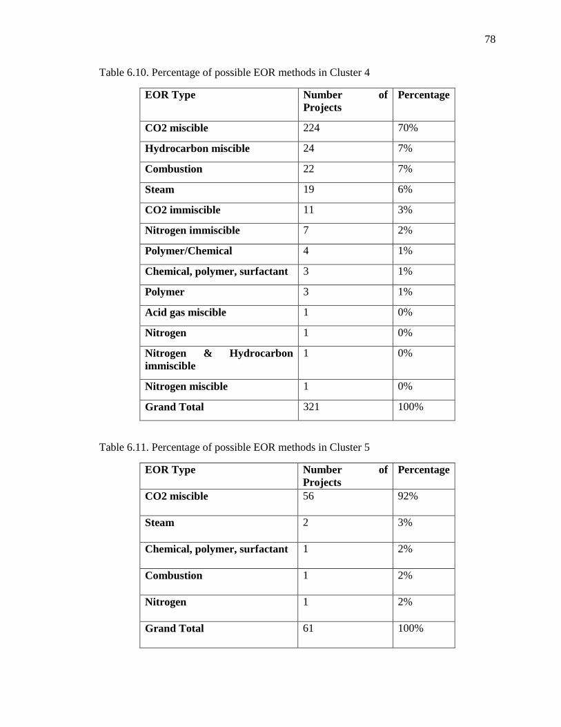
78


EOR Type Number of

Projects

Percentage

CO2 miscible 224 70%


Combustion 22 7%

Steam 19 6%

CO2 immiscible 11 3%




Polymer 3 1%

Acid gas miscible 1 0%

Nitrogen 1 0%

Nitrogen & Hydrocarbon

immiscible

1 0%

Nitrogen miscible 1 0%



EOR Type Number of

Projects

Percentage

CO2 miscible 56 92%

Steam 2 3%


Combustion 1 2%

Nitrogen 1 2%

Grand Total 61 100%

79


EOR Type Number of

Projects

Percentage



Nitrogen miscible 2 12%

Nitrogen & Hydrocarbon

immiscible

1 6%

Polymer 1 6%


Grand Total 17 100%

80

7. CONCLUSIONS

Results from the application of hierarchical clustering to the steam flooding and

worldwide EOR data set demonstrated the effectiveness of the approach to group data into

different clusters, and each cluster has different characteristics by using box plots and bar

charts. Based on the clustering results, screening criteria for steam flooding projects with

detailed analysis have been established based on categories, instead of the overall ranges

of a set of reservoir and fluid properties typically obtained in traditional screening criteria

studies. Inconsistent data is quickly filtered out into small clusters, which have 1-2 records

mostly.

Principal component analysis techniques are really helpful to analyze the data,

present the clustering results, and also to figure out the dominating features in both the

steam flooding projects and the worldwide EOR data set. The dominating features are

permeability, depth and viscosity for both data sets.

From the validation and prediction of the established method, a rapid with high

prediction accuracy method have been used which could save valuable time for decision

making, especially for mature reservoirs.

81

BIBLIOGRAPHY

1. Enhanced oil recovery, http://en.wikipedia.org/wiki/Enhanced_oil_recovery, 2015.

2. Manrique, E.J. and Pereira, C. A. 2007. Identifying Viable EOR Thermal Processes

in Canadian Tar Sands. Presented at the Canadian International Petroleum

Conference, paper # 2007-176, Calgary, Alberta, Canada.

3. Hama, M. Q., Wei, M., Saleh, L. D., & Bai, B. (2014, June 10). Updated Screening

Criteria for Steam Flooding Based on Oil Field Projects Data. Society of Petroleum

Engineers. doi:10.2118/170031-MS.

4. Al-Adasani, A., & Bai, B. (2010, January 1). Recent Developments and Updated

Screening Criteria of Enhanced Oil Recovery Techniques. Society of Petroleum

Engineers. doi:10.2118/130726-MS.

5. Alvarado, V., Ranson, A., Hernandez, K., Manrique, E., Matheus, J., Liscano, T.,

& Prosperi, N. (2002, January 1). Selection of EOR/IOR Opportunities Based on

Machine Learning. Society of Petroleum Engineers. doi:10.2118/78332-MS.

6. Enhanced Oil Recovery, http://energy.gov/fe/science-innovation/oil-gas-

research/enhanced-oil-recovery, 2015.

7. Shah, A., Fishwick, R., Wood, J., Leeke, G., Rigby, S. and Greaves, M., A review

of novel techniques for heavy oil and bitumen extraction and upgrading. Energy

Environ. Sci., 3, 700-714 (2010).

8. Sayyad, H., Khaksar Manshad, A., Rostami, H., 2014. Application of hybrid neural

particle swarm optimization algorithm for prediction of MMP. Fuel 116, 625-633.

9. In-situ combustion, http://petrowiki.org/In-situ_combustion, 2015.

10. Poettmann, F. H., & Hause, W. R. (1978, January 1). Micellar-Polymer Screening

Criteria And Design. Society of Petroleum Engineers. doi:10.2118/7068-MS.

11. Taber, J. J., Martin, F. D., & Seright, R. S. (1997, August 1). EOR Screening

Criteria Revisited - Part 1: Introduction to Screening Criteria and Enhanced

Recovery Field Projects. Society of Petroleum Engineers. doi:10.2118/35385-PA.

12. Guerillot, D. R. (1988, January 1). EOR Screening With an Expert System. Society

of Petroleum Engineers. doi:10.2118/17791-MS.

13. Saleh, L., Wei, M., & Bai, B. (2014, April 12). Data Analysis and Novel Screening

Criteria for Polymer Flooding Based on a Comprehensive Database. Society of

Petroleum Engineers. doi:10.2118/169093-MS.

http://energy.gov/fe/science-innovation/oil-gas-research/enhanced-oil-recovery

http://energy.gov/fe/science-innovation/oil-gas-research/enhanced-oil-recovery

82

14. Advanced Resources International (prepared for the U.S. DOE/NETL, Office of

Strategic Energy Analysis and Planning), Dis-aggregated Next Generation CO2

EOR, September 2013.

15. A Tutorial on Clustering Algorithms,

http://home.deib.polimi.it/matteucc/Clustering/tutorial_html/, 2015.

16. Hierarchical Clustering, http://en.wikipedia.org/wiki/Hierarchical_clustering, 2015.

17. Xu, Rui, and Don Wunsch. Clustering. Vol. 10. John Wiley & Sons, 2010.

18. Mohammadpoor, M., Qazvini Firouz, A. R., & Torabi, F. (2012, January 1).

Implementing Simulation and Artificial Intelligence Tools To Optimize the

Performance of the CO2 Sequestration in Coalbed Methane Reservoirs. Carbon

Management Technology Conference. doi:10.7122/151307-MS.

19. Al-Amer, A. A., Al-Nasser, N. bdulaziz, Al-Towaileb, H., Al-Gosayir, M. M., &

Al-Awadh, W. Y. (2014, December 10). Intelligent Field Real-Time Data

Reliability Key Performance Indices. International Petroleum Technology

Conference. doi:10.2523/17997-MS.

20. Park, H., Lim, J.-S., Kang, J. M., Roh, J., & Min, B. (2006, January 1). A Hybrid

Artificial Intelligence Method for the Optimization of Integrated Gas Production

System. Society of Petroleum Engineers. doi:10.2118/100997-MS.

21. Popa, A., Ramos, R., Cover, A. B., & Popa, C. G. (2005, January 1). Integration of

Artificial Intelligence and Lean Sigma for Large Field Production Optimization:

Application to Kern River Field. Society of Petroleum Engineers.

doi:10.2118/97247-MS.

22. Denney, D. (2011, October 1). Automating the Oilfield Asset - Artificial-

Intelligence-Based Integrated-Production-Management Architecture. Society of

Petroleum Engineers. doi:10.2118/1011-0091-JPT.

23. Cirilli, L. A. (2001, January 1). A New Alternative in the Performance Monitoring

and Control of the Reservoir- Artificial Lift System for the Optimization of a

Producing Well. Society of Petroleum Engineers. doi:10.2118/68700-MS.

24. Boomer, R. J. (1995, January 1). Predicting Production Using a Neural Network

(Artificial Intelligence Beats Human Intelligence). Society of Petroleum Engineers.

doi:10.2118/30202-MS.

83

25. Rebeschini, J., Querales, M., Carvajal, G. A., Villamizar, M., Md Adnan, F.,

Rodriguez, J., … Goel, H. K. (2013, October 28). Building Neural-Network-Based

Models Using Nodal and Time-Series Analysis for Short-Term Production

Forecasting. Society of Petroleum Engineers. doi:10.2118/167393-MS.

26. Ebrahimi, M., & Sajedian, A. (2010, January 1). Use of Fuzzy Logic for Predicting

Two Phase Inflow Performance Relationship of Horizontal Oil Wells. Society of


27. Ramgulam, A., Ertekin, T., & Flemings, P. B. (2007, January 1). An Artificial

Neural Network Utility for the Optimization of History Matching Process. Society

of Petroleum Engineers. doi:10.2118/107468-MS.

28. Bermudez, F., Carvajal, G. A., Moricca, G., Dhar, J., Md Adam, F., Al-Jasmi, A.,

Nasr, H. (2014, April 1). A Fuzzy Logic Application to Monitor and Predict

Unexpected Behavior in Electric Submersible Pumps (Part of KwIDF Project).

Society of Petroleum Engineers. doi:10.2118/167820-MS.

29. Mena, L., & Klein, S. (1999, January 1). Surface Axial Load Based Progressive

Cavity Pump Optimization System. Society of Petroleum Engineers.

doi:10.2118/53962-MS.

30. Stewart, G., & Du, K. F. (1989, January 1). Feature Selection and Extraction for

Well Test Interpretation by an Artificial Intelligence Approach. Society of


31. Allain, O., & Houze, O. P. (1992, January 1). A Practical Artificial Intelligence

Application in Well Test Interpretation. Society of Petroleum Engineers.

doi:10.2118/24287-MS.

32. Sung, W., Yoo, I., Ra, S., & Park, H. (1995, September 17). Development of HT-

BP Neural Network System for the Identification of Well Test Interpretation Model.


33. Aulia, A., Rahman, A., & Quijano Velasco, J. J. (2014, April 1). Strategic Well

Test Planning Using Random Forest. Society of Petroleum Engineers.

doi:10.2118/167827-MS.

34. Al-Kaabi, A. U., & Lee, W. J. (1993, September 1). Using Artificial Neural

Networks to Identify the Well Test Interpretation Model (includes associated

papers 28151 and 28165). Society of Petroleum Engineers. doi:10.2118/20332-PA.

35. Lim, J.-S., Kang, J. M., & Kim, J. (1998, January 1). Artificial Intelligence

Approach for Well-to-Well Log Correlation. Society of Petroleum Engineers.

doi:10.2118/39541-MS.

84

36. Jong-Se, L., Kang, J. M., & Jungwhan, K. (1999, January 1). Interwell Log

Correlation Using Artificial Intelligence Approach and Multivariate Statistical

Analysis. Society of Petroleum Engineers. doi:10.2118/54362-MS.

37. Olea, R. A., & Davis, J. C. (1986, January 1). An Artificial Intelligence Approach

to Lithostratigraphic Correlation Using Geophysical Well Logs. Society of


38. Whittaker, A. H., & Macpherson, J. D. (1986, January 1). Assistant Expert Log

Data Analysis System: Applications of Artificial Intelligence Programming

Techniques in Formation Evaluation. Society of Petrophysicists and Well-Log

Analysts.

39. Aulia, A., Rahman, A., & Quijano Velasco, J. J. (2014, April 1). Strategic Well

Test Planning Using Random Forest. Society of Petroleum Engineers.

doi:10.2118/167827-MS.

40. Sitouah, M., Al-Hamoud, M., Bougerira, Y., & Abdullatif, O. (2014, October 29).

Permeability Prediction in Carbonate Reservoirs using Specific Area, Porosity and

Water Saturation. Society of Exploration Geophysicists.

41. Mohaghegh, S., Arefi, R., Ameri, S., & Rose, D. (1995, December 1). Design and

Development of an Artificial Neural Network for Estimation of Formation

Permeability. Society of Petroleum Engineers. doi:10.2118/28237-PA.

42. Salazar, J. P., & Romero, P. A. (2001, January 1). NMR Measurements in

Carbonates Samples and Core-Logs Correlations Using Artificial Neural Nets.


43. Anifowose, F. A. (2012, January 1). Advances in Hybrid Computational

Intelligence Application in Oil and Gas Reservoir Characterization. Society of


44. Siena, M., Guadagnini, A., Rossa, E., Lamberti, A.L., Masserano, F., and Rotondi,

M. (2015). Development and Testing of Advanced Methods for the Screening of

Enhanced-Oil-Recovery Techniques. 18th European Symposium on Improved Oil

Recovery, April 2015.

45. Osman, E.-S. A., Ayoub, M. A., & Aggour, M. A. (2005, January 1). An Artificial

Neural Network Model for Predicting Bottomhole Flowing Pressure in Vertical

Multiphase Flow. Society of Petroleum Engineers. doi:10.2118/93632-MS

46. Kumar, A. (2012, April 30). Artificial Neural Network as a Tool for Reservoir

Characterization and its Application in the Petroleum Engineering. Offshore

Technology Conference. doi:10.4043/22967-MS.

85

47. Anifowose, F. A. (2012, January 1). Advances in Hybrid Computational

Intelligence Application in Oil and Gas Reservoir Characterization. Society of


48. Perez-Valiente, M. L., Martin Rodriguez, H., Santos, C. N., Vieira, M. R., & Embid,

S. M. (2014, April 1). Identification of Reservoir Analogues in the Presence of

Uncertainty. Society of Petroleum Engineers. doi:10.2118/167811-MS.

49. Roweis, S. T.; Saul, L. K. (2000). Nonlinear Dimensionality Reduction by Locally

Linear Embedding. Science 290 (5500): 2323–2326.

doi:10.1126/science.290.5500.2323. PMID 11125150.

50. Pearson Product-Moment Correlation Coefficient,

http://en.wikipedia.org/wiki/Pearson_product-

moment_correlation_coefficient#cite_note-4, 2015.

51. Vladimir, Alvarado, and Manrique Eduardo. Enhanced Oil Recovery: Field

Planning and Development Strategies, 2010.

52. Thomas, S. (2008). Enhanced oil recovery-an overview. Oil & Gas Science and

Technology-Revue de l'IFP, 63(1), 9-19.

53. Bourdarot, G., & Ghedan, S. G. (2011, January 1). Modified EOR Screening

Criteria as Applied to a Group of Offshore Carbonate Oil Reservoirs. Society of


54. Hierarchical Clustering

https://en.wikipedia.org/wiki/Hierarchical_clustering, 2015.

55. http://www.sjsu.edu/faculty/gerstman/StatPrimer/correlation.pdf, 2015.

56. Wagstaff, Kiri. Clustering with missing values: No imputation required. Springer

Berlin Heidelberg, 2004.

57. Pearson’s Correlation Coefficient

http://www.strath.ac.uk/aer/materials/4dataanalysisineducationalresearch/unit4/co

rrelationsdirectionandstrength/, 2015.

http://en.wikipedia.org/wiki/Digital_object_identifier

http://dx.doi.org/10.1126%2Fscience.290.5500.2323

http://en.wikipedia.org/wiki/PubMed_Identifier

http://www.ncbi.nlm.nih.gov/pubmed/11125150

86

VITA

Na Zhang was born in Hunan, China. She received her dual Bachelor of Science

degrees from Missouri University of Science and Technology and China University of

Petroleum in May, 2013. After that, she continued study at Missouri University of Science

and Technology, and was employed as a graduate assistant under Dr. Mingzhen Wei from

2013 to 2015. She earned her Master’s degree in Petroleum Engineering from Missouri

University of Science and Technology in December, 2015.

Steam flooding screening and EOR prediction by using ...

Documents

Transcript of Steam flooding screening and EOR prediction by using ...