STEAM EMISSIONS OF UC CAMPUS: MITIGATING CLIMATE IMPACTS · PDF fileSTEAM EMISSIONS OF UC...

1 | P a g e

STEAM EMISSIONS OF UC CAMPUS: MITIGATING CLIMATE IMPACTS UC Berkeley Climate and Greenhouse Gas Emissions Research/Analysis

Presented By: Angela Cheng: [email protected] Emun Davoodi: [email protected] Tiffany Deng: [email protected] Daniel Shen: [email protected]

December 2012 CE 268E - Civil Systems and the Environment

2012

mailto:[email protected]



2 | P a g e

Table of Contents ABSTRACT .................................................................................................................................................. 4

EXECUTIVE SUMMARY .......................................................................................................................... 4

UNITS ........................................................................................................................................................... 7

SCOPE .......................................................................................................................................................... 8

INTRODUCTION ........................................................................................................................................ 9

PROBLEM STATEMENT ......................................................................................................................... 14

BACKGROUND ........................................................................................................................................ 14

APPROACH/MODEL ................................................................................................................................ 18

FINDINGS AND RESULTS ...................................................................................................................... 26

SENSITIVITY ANALYSIS ....................................................................................................................... 30

UNCERTAINTY ASSESSMENT AND MANAGEMENT ...................................................................... 33

INTERPRETATION AND DISCUSSION OF RESULTS ........................................................................ 35

CONSTRAINTS ......................................................................................................................................... 39

RECOMMENDATIONS ............................................................................................................................ 40

CONCLUSIONS......................................................................................................................................... 44

REFERENCES ........................................................................................................................................... 45

3 | P a g e

Figure 1. Process diagram of the scope of this project analysis. ................................................................... 8

Figure 2. Cogenertaion Plant Flow Chart ................................................................................................... 11

Figure 3. Sensitivity Test on Natural Gas Loss (Spath & Mann, 2000). .................................................... 17

Figure 4. Stanford Cogeneration Process 2010 Emission Inventory .......................................................... 18

Figure 5. UC Berkeley Campus Steam Consumption 2006-2011 .............................................................. 19

Figure 6. Life Cycle GWP of a Natural Gas Combined-Cycle Power Generation System ........................ 21

Figure 7. Koshland Hall Steam Consumption (in lbs) from July 2011 to June 2012 ................................. 24

Figure 8. Wurster Hall Steam Consumption (in lbs) from July 2011 to June 2012 .................................... 24

Figure 9. Koshland Hall and Wurster Hall Steam Consumption (in lbs) from July 2011 to June 2012. .... 25

Figure 10. Annual Steam Emission (2006 - 2011) ...................................................................................... 26

Figure 11. Annual Steam Emission From 2006 to 2011 ............................................................................. 27

Figure 12. Hourly emissions for the heating case study. ............................................................................ 28

Figure 13. Hourly costs for the heating case study ..................................................................................... 29

Figure 14. Sensitivity Analysis - CO2 Emission Variation due to Changing % Total Energy in Steam .... 31

Figure 15. Sensitivity Analysis - CO2 Emission Variation due to Changing Cogeneration Plant Power

Efficiency .................................................................................................................................................... 32

Figure 16. Sensitivity Analysis - CO2 Emission Variation due to Changing Auxilary Boiler Efficiency . 32

Table 1. GWP Contribution of Each Component in Natural Gas Combined Cycle Power Plant ............... 15

Table 2. Sensitivity Test on Natural Gas Loss (Spath & Mann, 2000). ...................................................... 16

Table 3. Emission Factor in 2006 and 2008 Protocol (General Reporting Protocol, 2008). ...................... 20

Table 4. Areas of Koshland and Wurster Hall (in square feet) (UC Berkeley FacilitiesLink, 2012) ......... 23

Table 5. Calculating the percent difference in square footage gives: ......................................................... 24

Table 6. Steam Emission Factors from Protocols and LCA ....................................................................... 27

Table 7. Heat Case Study - Energy Emission and Costs Per Hour ............................................................. 28

Table 8.Conversion Factors: Steam versus Electricity ............................................................................... 29

Table 9. Powering a single autoclave in Koshland Hall in one year ........................................................... 30

Table 10. Uncertainty Level of the Information ......................................................................................... 33

4 | P a g e

ABSTRACT In compliance with CalCAP’s (Cal Climate Action Partnership) 2007 feasibility study and Chancellor

Birgeneau’s commitment to the university, UC Berkeley has aimed to reduce its greenhouse house gas

(GHG) emissions to 1990 levels by the year 2014. According to the UC Berkeley Campus sustainability

report 2011, steam is one the top three emission sources and contributes about 41% of the total emissions,

which is even 10% higher than the emissions contributed from purchased electricity, making steam the

largest source of emissions. The steam is used on campus to heat and cool buildings and water, and

emissions are continuing to grow.

This study aims at evaluating the methodologies currently used on campus in order to pinpoint

adjustments for improvement and to help determine whether or not the campus should continue

purchasing steam in the same manner from the nearby Cogeneration plant when its current contract

expires in 2017. Two buildings on campus, Koshland Hall and Wurster Hall, have been chosen for direct

case studies for analysis. Additionally, alternatives such as purchasing electricity from PG&E are used as

comparisons for heating the buildings and for powering the lab equipment. When GHG emissions through

steam emission reductions prove to be infeasible or unreasonable, reducing GHG emissions from other

sources is considered.

EXECUTIVE SUMMARY In UC Berkeley’s campus, steam is used for a variety of purposes such as heating, cooling, and running

equipment in labs. Steam is generated by a third party-owned cogeneration plant, also known as a natural

gas combined cycle plant, and it is purchased in 1000 pound increments by the campus. Additionally, UC

Berkeley owns and operates three auxiliary boilers that supplement the campus steam supply under high

demands.

UC Berkeley consumes an average of 706 million pounds of steam per year, which amounts to roughly

$5.7 million dollars worth of annual steam. This is a large figure, and being that steam is the largest

contributor, contributing to 41% of current campus greenhouse gas emissions (GHGs), UC Berkeley

sought out solutions to mitigate the carbon emissions associated with steam generation. This study

inspects the current steam system as well as a couple of case studies to determine whether or not steam is

the optimal choice for energy, followed by concrete recommendations to the campus about how the

current steam system can and should be improved.

The authors begin the environmental analysis of steam usage in Berkeley by first confirming that the

reported campus data are accurate. UC Berkeley’s sustainability office was able to provide the metered

5 | P a g e

value of steam and electricity production from Berkeley’s Delta Cogeneration Plant, along with the

estimated results of carbon dioxide emissions based on inputs of natural gas energy. Since the

methodology used for the calculation is from 2006, the authors compared the results to a more recent

protocol from 2008. Based on detailed calculations, the end results of the two protocols yielded

essentially the same results for cogeneration plant emissions: 180g CO2 eq. per kWh generated for the

2006 protocol versus 181 g CO2 eq. per kWh generated for the 2008 protocol.

With the use of similar studies in cogeneration plants, focusing on both usage and emissions (related to

global warming potential in the case of this analysis), the authors are able to draw certain conclusions

about UC Berkeley’s cogeneration plant. The first study looks at an analysis of a large, 505 megawatt

cogeneration plant and the global warming potential that is associated with the plant in its lifetime. This is

called a life-cycle assessment (LCA), which takes the viewpoint of ‘cradle to the grave’ emissions of the

whole lifecycle of a cogeneration plant. The total LCA GWP for cogeneration plants based on this study

is 499g CO2 eq. per kWh. From this, it is evident that about three quarters of the carbon emissions came

from operating the plant, and a quarter of the total emissions was associated with natural gas production

and distribution. In addition, this National Renewable Energies Laboratory analysis also indicated that the

fugitive losses of natural gas can have a relatively decent impact on the overall global warming impact;

thus mitigating the fugitive losses would be of good interest. It is important to note, however, that the

emissions associated with steam generation at a cogeneration plant is based on energy content. That being

the case, 51-65% of the 499g CO2 eq. per kWh are associated with steam generation; this values to 255-

325g CO2 eq. per kWh on an LCA basis. A similar study is looked at for the campus-owned auxiliary

boilers, and the LCA value was determined to be 302g CO2 eq. per kWh of steam generated.

Additionally, the authors look at two campus buildings to serve as case studies for steam use analysis.

Koshland and Wurster Halls are the selected two buildings with Koshland Hall being the more recently

built bio-sciences lab building and Wurster Hall being the older mixed-use building. From steam

consumption data, it is apparent that Koshland Hall uses roughly 10 times the steam that Wurster Hall

uses. This is attributable to the fact that Koshland Hall is a lab building, of which are known to consume

large amounts of energy, namely, steam.

In order to analyze the steam, a couple of case studies are generated to compare different forms of energy.

The first case study looks into the heating of Koshland and Wurster Halls, and based on area, because

Wurster Hall is much larger than Koshland Hall, Wurster consumes more energy in this analysis. By

comparing steam to PG&E mix electricity and natural gas on emissions and cost basis, it is evident that

6 | P a g e

steam is far superior in both areas when compared to its competitors. Therefore, steam is deemed the

number one option for heating.

Next, autoclaves are investigated. Autoclave is a piece of lab equipment that uses large amounts of steam

to sterilize objects. Koshland Hall has 12 of these, the energy use of the autoclaves is looked at using

steam and PG&E mix electricity. Once again, looking at both emissions and costs, steam is a far better

option than the alternative, and this further implants the idea that steam is the best solution for the

campus.

After some sensitivity analyses to look at different scenarios, and uncertainty analyses to examine data

quality, the final step is to come up with tangible solutions that the UC Berkeley can benefit from. Since

steam is purchased based on demand, the main idea is to reduce that demand. By increasing the end-user

efficiency in the buildings, the steam drawn in will be reduced leading to lessened emissions. This can be

done by simply updating equipment to newer more efficient items. In turn, using less steam reduces the

use of the auxiliary boilers, also reducing emissions. At the opposite end of the spectrum, increasing the

cogeneration plant efficiency, despite the fact that UC Berkeley does not own the plant, will reduce

emissions as well. This can be done in a number of ways, the simplest being a modification to the turbine

with tighter seals. The auxiliary boilers, in turn, can be improved as well if they are chosen not to be

updated, and adding vent dampers to the system is a cost-effective and emissions-reducing solution,

amongst other possibilities.

Finally, the authors conclude the report with suggestions for the expiration date of the 30-year contract

between UC Berkeley and the cogeneration plant owners, which is in 2017. In short, the authors

recommend keeping the plant running, but strongly discourage the university from taking over the plant,

because UC Berkeley is better off not assuming the responsibilities for the power plant’s emissions,

maintenance, and operation. Instead, the authors suggest the university extend the contract with the

cogeneration plant, at least for a short term, until a concrete solution is formulated - so far, no thoughts

are percolating about what could be done. The other solution is for the campus to aid the plant financially

in improving the equipment, with the possibility of taking a partial stake in ownership of the plant, but not

in such a way that the university would be responsible for operating or maintenance costs. This option

allows both UC Berkeley and the cogeneration plant owner to be associated with reduced carbon

emissions. The options are plentiful for reducing emissions; the only constraint is in the decision makers

to formulate what they think are the best feasible options.

7 | P a g e

UNITS Metric units are used in this report for mass, mass of emissions and electricity usage; however, English

units are used for energy, steam usage and pressure.

Mass: gram (g) or kilogram (kg)

Global Warming Potential (GWP): kilograms or mega grams/metric tons of carbon dioxide equivalence

(kg CO2e or Mg CO2e/MT CO2e)

Energy: million British thermal units (MMBtu)

Electricity Usage: kilowatt hours (kWh)

Electricity Production: megawatts (MW)

Steam Consumption: pounds of steam (lbs.)

Pressure: pounds per square inch, gauge (psig)

Cost: US dollars ($)

8 | P a g e

SCOPE The scope of this report included steam generation at the cogeneration plant and the auxiliary boilers, and

the emissions associated with those utility providers. The transportation of steam into the buildings, in

the case of this report, Koshland and Wurster Halls. Finally, both Koshland and Wurster Halls were

looked at as case studies for heating and heating alternatives, and autoclaves and lab energy

alternatives. In the heating case, natural gas and PG&E electricity mix were compared with steam, and in

the autoclave case study, PG&E electricity mix was compared to steam. A process diagram of the project

scope can be observed in figure 1.

Figure 1. Process diagram of the scope of this project analysis.

9 | P a g e

INTRODUCTION

The Purpose of Steam Steam is used in the UC Berkeley campus for heating, cooling and for running various pieces of lab

equipment (e.g. autoclaves use steam to sterilize objects). The steam generated by the cogeneration plant

and UC Berkeley’s auxiliary boilers is used to feed the main campus, with some of the steam traveling to

a few buildings outside the main campus (e.g. Soda Hall). The fact that steam is so vastly used for a large

variety of purposes on campus makes the steam very necessary for UC Berkeley. Without the steam there

would have to be a large infrastructure upgrade to feed the alternative that would replace the steam - so if

natural gas was selected as a steam replacement for a building’s heating, new natural gas lines would have

to be installed from the main line on the streets of Berkeley to feed that alternative.

The UC Berkeley consumes over 706 million pounds of steam a year, and this is equivalent to about $5.7

million dollars in steam costs alone, each year. The UC Berkeley cogeneration plant can deliver up to

185,000 pounds of steam per hour, and the campus buys steam in 1000 pound increments (Lipman, 2011)

& (G. Escobar, personal communication, November 15, 2012). Each of the three auxiliary boilers can

deliver up to 80,000 pounds of steam per hour, but this steam is not purchased by the campus, just

generated (UC Berkeley Facilities Services, 2003). This being the case, steam plays a very central role in

the campus utility system, as well as the campus budget system. The campus, however, does have the

opportunity to lower this consumption and improve the cost if certain actions are taken to do

so. Recommendations for improvement to the steam system are presented toward the end of this report,

and they are aimed at lowering consumption, costs, and ultimately, the GHG emissions associated the

steam generated.

Cogeneration Plant Before 1987, steam needed for the UC Berkeley campus was supplied by a boiler plant, which consisted

of four boilers powered by natural gas or oil. The steam is used on campus for heating buildings and

water and cooling buildings by means of absorption chillers. It is delivered on-tap for lab purposes. Being

that electricity is purchased from PG&E, the campus sought out a system that would provide UC

Berkeley with both steam and electrical power. As a result, the campus eventually developed a plan for a

cogeneration plant that could accomplish this. The campus went through a number of different options

and ultimately decided to buy steam from a cogeneration plant, owned and operated by a third party. The

plant would be supplied to the campus with electricity, and all other electricity generated would be sold to

PG&E, otherwise. Eventually, the first of the four original boilers was removed to make room for this

10 | P a g e

cogeneration plant, which is now situated near Haas Pavilion on the southwest corner of campus (UC

Berkeley Facilities Services, 2003).

UC Berkeley’s steam demand fluctuates from 50,000 pounds per hour (pph) to about 240,000 pounds per

hour. This demand can be met by the cogeneration plant, for the most part, but at higher necessity the use

of the auxiliary boilers aids the cogeneration plant (the auxiliary boilers are also used when the

cogeneration plant is offline). The auxiliary boilers consist of the three remaining original boilers, since

the fourth was removed for the construction of the cogeneration plant. These boilers were originally rated

at about 100,000 lbs. per hour, but after the promulgation of stricter emissions regulations, the auxiliary

boilers were modified to output steam at about 80,000 pph. These three remaining boilers are still owned

and operated by UC Berkeley (UC Berkeley Facilities Services, 2003).

The cogeneration plant is operational all year long, 24 hours a day, with the exception of breakdowns or

when maintenance requires it to be offline. There is a full crew that works at the plant, and they operate

the plant interminably. Steam is piped to all of the central campus buildings, as well as a select few on

the perimeter, at a pressure of about 120 pounds per square inch gauge (psig), and the heat recovery steam

generator (HRSG) can provide about 80,000 pph of steam (almost double that can be supplied when the

duct burners between the turbine and HRSG are fired). The main generator can produce about 25

megawatt (MW) of electricity, and the steam generator can provide between 1.5 and 4.5 MW (parasitic

loads of the plant are about 1 MW). With the implementation of steam augmentation, a configuration that

allows steam to be injected into the combustion chamber of the gas turbine to increase the mass flow and

total output, the main generator can reach 26.4 MW (the steam augmentation took the place of water

injection for better emissions control). This power output, however, is limited not by the unity power

factor, but by the campus power factor of 0.85 (UC Berkeley Facilities Services, 2003). A detailed flow

diagram for steam generation and usage is illustrated in figure 2 below.

Steam Usage & Non-Usage As mentioned earlier, the campus steam is used year round for temperature control as well as for lab

equipment, such as glass washers. That being the case, the campus has its own strategic way of trying to

save on its energy bill. According to the campus utilities manager, Gilbert Escobar, the use of an

absorption chiller, an air conditioning device that is mainly powered by the energy in the delivered steam,

is used in the summer time when natural gas is cheaper to buy than electricity. Being that most of the

buildings, especially the newer ones, are fitted with two types of chillers, the use of an electric powered

chiller (also a device used to cool the air in a building) is more common during winter time, when

electricity is cheaper than natural gas (yearly average of electricity is about $0.11/kWh). Nevertheless,

11 | P a g e

Escobar mentions that, in most cases, the use and implementation of chillers are excessive. Escobar says

that simply bringing in fresh outdoor air, or comfort cooling, rather than air conditioning, would not only

be just as effective, but it will also be cheaper and less polluting. This, of course, may not be applicable

during the hotter days of the year; however, for the mild climate in Berkeley, CA, this strategy would

likely be more useful than not (G. Escobar, personal communication, September 24, 2012).

Figure 2. Cogeneration Plant Flow Chart

The heating units are basic air handlers or radiators, and run on steam regardless. On the heating side of

the climate control realm, a lot of steam is left dormant in buildings where it is not actually used until it is

fairly cold outside. This is a waste because the steam loses its heating energy regardless of whether or not

it is being used to heat the building after it is piped to it. In addition, many of the buildings on campus are

fairly old and not insulated properly. Thus, if there were proper insulation, then the use of the dormant

steam may not even be necessary on any day of the year (G. Escobar, personal communication,

September 24, 2012).

Cogeneration Systems & GWP The cogeneration plant is run in a combined cycle. Essentially, a jet engine run on natural gas (GE LM-

2500) powers the main electric generator; this is the same engine that is placed in a commercial DC-10

and military C5A aircraft (the turbine can also run on fuel oil number 2, which can be used in emergency

situations as it is more impractical than natural gas). Natural gas is provided to the cogeneration plant at

12 | P a g e

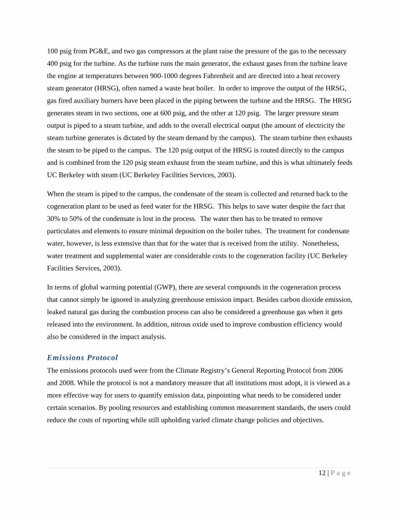
100 psig from PG&E, and two gas compressors at the plant raise the pressure of the gas to the necessary

400 psig for the turbine. As the turbine runs the main generator, the exhaust gases from the turbine leave

the engine at temperatures between 900-1000 degrees Fahrenheit and are directed into a heat recovery

steam generator (HRSG), often named a waste heat boiler. In order to improve the output of the HRSG,

gas fired auxiliary burners have been placed in the piping between the turbine and the HRSG. The HRSG

generates steam in two sections, one at 600 psig, and the other at 120 psig. The larger pressure steam

output is piped to a steam turbine, and adds to the overall electrical output (the amount of electricity the

steam turbine generates is dictated by the steam demand by the campus). The steam turbine then exhausts

the steam to be piped to the campus. The 120 psig output of the HRSG is routed directly to the campus

and is combined from the 120 psig steam exhaust from the steam turbine, and this is what ultimately feeds

UC Berkeley with steam (UC Berkeley Facilities Services, 2003).

When the steam is piped to the campus, the condensate of the steam is collected and returned back to the

cogeneration plant to be used as feed water for the HRSG. This helps to save water despite the fact that

30% to 50% of the condensate is lost in the process. The water then has to be treated to remove

particulates and elements to ensure minimal deposition on the boiler tubes. The treatment for condensate

water, however, is less extensive than that for the water that is received from the utility. Nonetheless,

water treatment and supplemental water are considerable costs to the cogeneration facility (UC Berkeley

Facilities Services, 2003).

In terms of global warming potential (GWP), there are several compounds in the cogeneration process

that cannot simply be ignored in analyzing greenhouse emission impact. Besides carbon dioxide emission,

leaked natural gas during the combustion process can also be considered a greenhouse gas when it gets

released into the environment. In addition, nitrous oxide used to improve combustion efficiency would

also be considered in the impact analysis.

Emissions Protocol The emissions protocols used were from the Climate Registry’s General Reporting Protocol from 2006

and 2008. While the protocol is not a mandatory measure that all institutions must adopt, it is viewed as a

more effective way for users to quantify emission data, pinpointing what needs to be considered under

certain scenarios. By pooling resources and establishing common measurement standards, the users could

reduce the costs of reporting while still upholding varied climate change policies and objectives.

13 | P a g e

Koshland and Wurster Halls To represent the different types of buildings on campus, the authors selected Koshland Hall and Wurster

Hall as campus building case studies. Koshland Hall is a laboratory type building as is Lewis, Tan,

Latimer, and many other buildings. On the contrary, Wurster houses a dining facility as well as

classrooms and large areas for studio. Thus, Wurster Hall is an appropriate case study for other classroom

type buildings such as Barrows, Dwinelle, and Wheeler Halls. Due to the lack of the utility equipment

logs, however, information necessary to thoroughly analyze the buildings is not present, so a rudimentary

comparison was made between the two buildings.

The data that was available shows that Koshland Hall consumes about ten times more Steam than Wurster

Hall, albeit its area is about 70% of Wurster’s. Koshland Hall has much more lab equipment, such as

fermenters, glasswashers, and autoclave jackets that require steam to operate, so the difference in steam

consumption is likely not attributable to the general heating of the building. Rather, it is likely due to the

fact that the two buildings are used for different purposes with Koshland Hall being a bioscience lab

building.

Two studies are conducted, both of which look into alternative sources of energy. The first study focuses

on the heating of the buildings on an average cold day in Berkeley, California, or in other words, heating

the buildings from 42 degrees Fahrenheit to 68 degrees Fahrenheit. A comparison was made among the

different alternatives: steam, electricity, and natural gas by evaluating the greenhouse gas emissions and

the costs of steam and of the alternatives.

The second study took a glimpse into lab equipment, particularly the autoclaves and the costs and

emissions associated with them. This was deemed worthwhile because Koshland has a total of twelve

autoclaves. Total cost and greenhouse gas emissions were calculated and compared between steam and

electricity from PG&E.

Afterwards, a sensitivity analysis and an uncertainty assessment are conducted. This helps analyze the

data that is obtained and establishes the quality of the data collected. Although the issue at hand for the

university is not a simple one to resolve, and this report cannot and does not incorporate every possible

option and alternative; the report, nevertheless, has enough for the authors to offer many suggestions for

improvement. In summary, the authors are hopeful that the university will consider the analyses and

recommendations presented here for the betterment of the university, and society as a whole.

14 | P a g e

PROBLEM STATEMENT

Steam consumption in UC Berkeley’s campus is one of Berkeley’s largest contributors to greenhouse gas

emissions. The emissions are shared with the electricity production at the cogeneration plant, but this

sharing may not be the best way to supply the campus with on-tap steam, heating, and cooling. Thus, the

authors analyzed the current steam usage to help determine if there are better alternatives.

The campus is still growing in size, albeit at a slow rate, and the construction of new buildings along with

the addition of students and faculty increases the demand for steam. Currently, the campus steam supplied

by the cogeneration plant cannot meet the campus’ needs when there is a high demand for heating,

cooling, or on-tap steam, so whenever the steam supplied by the cogeneration plant is insufficient, the

auxiliary boilers are utilized. Even with the supplementary auxiliary boilers, however, the campus is

coming close to reaching its capacity with steam generation, and the fact that the campus is gradually

growing can only worsen this effect; all of this is associated with large amounts of GHG emissions (UC

Berkeley Facilities Services, 2003).

In order to resolve the issue as a whole, some smaller concerns need to be addressed. First, the method

used to calculate emissions has to be examined to see if it is the best representation for the steam

emissions in UC Berkeley’s campus. Then, the campus steam generation methods can be analyzed and

compared to other alternatives that may be better for the campus’ set-up, such as electricity and natural

gas. Alternatives to the current steam generation method exist, but the authors believe that a thorough

analysis, through means of an LCA (life cycle assessment) and several campus case studies, is necessary

to reveal the optimal solution.

BACKGROUND

505 MW Cogeneration Plant Study According to Spath and Mann (2000) carbon dioxide (CO2) accounts for over 99% of all air emissions in

cogeneration facilities, measured by weight. Focusing on global warming potential, the next highest-

emitting gas contributing to global warming is methane (CH4), followed by trace amounts of nitrous oxide

(N2O). These three greenhouse gases are used for GWP assessment of the system. The

Intergovernmental Panel on Climate Change classifies GWP in terms of carbon dioxide equivalents, CO2e,

and the assigned capacities for a 100-year time frame for methane and nitrous oxide are 21 and 310 times

greater than CO2, respectively (Spath & Mann, 2000).

15 | P a g e

In analyzing a much larger scale version (505 MW) of the cogeneration plant positioned in Berkeley’s

campus, Spath and Mann (2000) came up with results for the GWP of each system component associated

with a natural gas combined cycle (NGCC) for electricity generation. The whole upstream operation

system was generalized into the following main processes: construction & decommissioning of the power

plant, construction of the natural gas pipeline, and natural gas production and distribution. The results can

be seen in Table 1 below. One difference between UC Berkeley’s plant and the plant that Spath & Mann

(2000) analyzed is the use of ammonia. The ammonia is used for NOX removal and plant operation, and

that is not considered in the analysis in this report; this, however, is a very minimal fraction of the total

(Spath & Mann, 2000). In the life cycle assessment (LCA), all upstream operations mentioned above were

considered when evaluating and quantifying the environmental aspects of producing electricity. The LCA

value, therefore, encompasses more factors than basic emission values.

Table 1. GWP Contribution of Each Component in Natural Gas Combined Cycle Power Plant

Table 1 above indicates the amount of greenhouse gas emissions or CO2e that exists for the construction,

operation, and decommissioning of such a plant. This is a sort of life-cycle assessment analysis that was

performed to break down the GHG emission per unit of electricity that is generated by the given

plant. Plant operations clearly take part in the largest part of GHG emission in the life-cycle of such a

plant, with the production and distribution of natural gas comprising a third of that. Therefore, improving

these areas can effectively improve the system as a whole.

In the case that was worked on in Spath and Mann (2000) a fugitive loss of 1.4% for natural gas that is

extracted was assumed. When considering the life-cycle of the ‘whole’ system, this is

significant. Natural gas has benefits as a fuel over resources like coal, because no solid waste is emitted,

but using natural gas as an energy source is still a concern, as it is nonrenewable. Natural gas contains

Note: The construction and decommissioning subsystem includes power plant construction and decommissioning as well as

construction of the natural gas pipeline (Spath & Mann, 2000). Also note that ammonia production and distribution is

striked-out because it is available in the 505MW case study, but not in UC Berkeley’s application. It was just displayed to

show how the 499 g CO2 eq. was calculated.

16 | P a g e

mostly methane (CH4), which induces higher radiative forcing than does carbon dioxide, thus making

fugitive losses a relatively significant contribution to GHG emission of the plant (methane also contains

ethane and trace amounts of propane and carbon dioxide, among other compounds). Spath and Mann

(2000) analyzed a typical window of fugitive natural gas losses, and determined it was 0.5% at the low

end and 4% at the high end (with their base case being the 1.4%). Table 2 below shows that a minor

change in natural gas losses leads to a significant change in the overall GHG emission of the system

(Spath & Mann, 2000).

Table 2. Sensitivity Test on Natural Gas Loss (Spath & Mann, 2000).

As can be seen, the small amount of increased fugitive emissions will increase the overall GHG emissions

a great deal, while it masks the effects of the other categories (larger natural gas loss artificially lessens

how ‘bad’, say, emissions from the power plant look, because that fraction of the total is smaller as a

result). Thus, mitigating the amount of lost natural gas to the atmosphere would be a way to lower any

system’s total emission (Spath & Mann, 2000).

Case Studies done by Other Universities’ Sustainability Group (Stanford, NYU,

University of Miami) Analogous to CalCAP’s report in emissions inventory, several groups provided similar information in

regards to where the emission sources came from. However, the categorization in which they accounted

for greenhouse emissions due to the cogeneration plant is completely different.

NYU’s group has assumed that the greenhouse gas emissions due to cogeneration should be calculated

from the source used, rather than from the resulting energy products (electricity and steam). In that case,

the percentage of carbon emissions due to steam is only 4%, which is purchased from New York City

utilities, as shown in Figure 3.

http://sustainablestanford.stanford.edu/emissions_inventory

http://www.nyu.edu/sustainability/pdf/capreport10.pdf

17 | P a g e

Such methodology Such methodology may suggest

that, if CalCAP decides to report the emissions

inventory of UC Berkeley based on the energy

sources instead, the emissions due to steam would

“appear” to be much smaller. However, the validity

of such a justification should be questioned,

whether or not accounting emissions based on the

sources is better or worse in illustrating the

university’s challenge in reducing carbon emissions.

If the university aims to reduce energy

consumption in the campus, it would require

information such as how and what type of the

energy is used, otherwise it would not be able to

publish relevant guidelines for university members

to follow. With that in mind, NYU’s breakdown

does not indicate what individuals should look out

for when they utilize any forms of energy.

Comparatively, Stanford’s sustainability group

represents GHG emission data related to

cogeneration plant operation with a few categories

of its own (university system/ hospital system).

Including all sectors of emission, Stanford’s total

emission is about 270,000 metric tons of CO2e.

Stanford termed its combined heating and power

system “cardinal cogen”, which consists of the

following components: a boiler plant, a chilled water plant, a cogeneration plant, and an ice plant. Similar

to the cogeneration and auxiliary boiler system in UC Berkeley, each plant operates based on current

demand, and provides backup steam in case the main cogeneration plant is not operational for any reasons.

The interesting aspect of Stanford’s system has to do with the chilled water plant, which operates the

steam-powered chiller, using excess steam generated by the cogeneration plant during the summer, when

campus steam loads are low and electrical rates are high.

Adding every element together, the cogeneration in Stanford accounts for 70% of the total CO2 emissions.

While the graph in Figure 4 clearly indicates that the cogeneration process is the main contributor in the

Figure 3. Sensitivity Test on Natural Gas Loss (Spath & Mann, 2000).

Note: the natural gas value in the pie chart in the lower

figure should be 39,000 MTCE (143,000 ton CO2 eq.).

18 | P a g e

Stanford campus, it would be more desirable if the emissions inventory for university cardinal cogen is

broken down even further.

Figure 4. Stanford Cogeneration Process 2010 Emission Inventory

University of Miami has done an analysis on their steam piping system in order to reduce the heat loss

during transportation of steam. Before having the better insulation in their piping system, they had

observed 12-15 million pounds of steam loss, which translates to $65,000 loss monthly. They found that

by having different insulation, ranging from uncoated fiberglass sheet, high-temperature fiberglass to foil-

faced fiberglass, and 40% to 64% of energy saving could be achieved. With an old steam tunnel system in

UC Berkeley campus underground, high leakage and heat loss are expected to be seen in the steam piping

system. Therefore, environmental cost and energy loss should be assessed for transporting steam from the

power generation plant to the campus. Based on the results, improvements should be suggested to reduce

steam loss during transportation in the steam tunnel system (Duffy, G.K., 2010).

APPROACH/MODEL

UC Berkeley knows the natural gas emission readings from the auxiliary boiler as well as the total usage

of natural gas in its facilities. The cogeneration plant was assumed to have produced the rest of the steam.

Thus, assuming that the readings from the auxiliary boiler are accurate, the amount of steam produced

from the cogeneration plant would be the difference between the total steam usage and the amount

produced by the auxiliary boiler.

SU- Stanford University

SHC-Stanford Hospital Clinic

LPCH- Lucile Packard Children

Hospital

19 | P a g e

The following Figure 5 shows the breakdown between the cogeneration plant and the auxiliary boiler of

steam consumption over time. Note that the majority of the steam used is produced by the cogeneration

plant.

Figure 5. UC Berkeley Campus Steam Consumption 2006-2011

The UC Berkeley Campus committed to reducing its global warming potential (GWP) to 1990 levels by

2014. Recall that the natural gas emission readings and the overall steam usage of UC Berkeley from

January 2006 to December 2011 is known. However, 1990 greenhouse gas emission levels are unknown.

Now, it is 2012, and from the 2006 to 2011 data, UC Berkeley’s greenhouse gas emissions have increased

by about 6%.

Assuming that the greenhouse gas emissions followed the same trend from 1990 to 2006, UC Berkeley

has definitely strayed further away from the 1990 levels of greenhouse gas emissions.

Estimating Greenhouse Gas Emissions in CO2 Equivalence In order to estimate the GWP, UC Berkeley used the Climate Registry’s General Reporting Protocol from

2006. Carbon dioxide equivalent emissions were recalculated by the authors using the same protocol.

They also calculated the emissions using the Climate Registry’s General Reporting Protocol from 2008.

This new protocol was slightly different in how it converted natural gas to MMBtu.

The conversion rates from natural gas to MMBtu in the 2006 protocol were 52.78 kg CO2/MMBtu,

0.0059 kg CH4/MMBtu, and 0.0001 kg N2O-/MMBtu, as shown in Table 3. After converting the methane

and nitrous oxide to CO2 equivalence, the emission factor is 54.05 kg CO2/MMBtu.

0.00E+00

2.00E+04

4.00E+04

6.00E+04

8.00E+04

1.00E+05

1.20E+05

1.40E+05

Jan-2006 Apr-2007 Jul-2008 Oct-2009 Jan-2011

Stea

m C

onsu

mpt

ion

(mm

BTU

)

Total Steamconsumption(mmBTU)

Steam Consumption(mmBTU) Aux Only

Steam Consumption(mmBTU) CogenOnly

20 | P a g e

Table 3. Emission Factor in 2006 and 2008 Protocol (General Reporting Protocol, 2008).

Fuel Gas Emitted Emission Factor in 2006

Protocol

Emission Factor in 2008

Protocol

Natural Gas Carbon Dioxide 52.78 kg/MMBtu 53.06 kg/MMBtu

Natural Gas Methane 0.0059 kg/MMBtu 0.001 kg/MMBtu

Natural Gas Nitrous Oxide 0.0001 kg/MMBtu 0.0001 kg/MMBtu

Compared with the old protocol, the 2008 protocol assumes that natural gas has more kg/MMbtu of CO2

than before, which changes the emission factor to 54.33 kg CO2/MMBtu. This implies that the

calculations from the old protocol have slightly underestimated values of kg of CO2 and the total

greenhouse gas emission.

Environmental Cost of Steam Usage Although the difference between emission factors may seem insignificant, the large amounts of natural

gas used each month adds up over time due to the high consumption.

Estimation of environmental impact of steam usage in UC Berkeley has been done by calculating the

GWP of burning natural gas. However, authors suggested that an analysis of environmental impact of

steam usage should be done on a complete steam production and usage process, including natural gas

usage, transportation of steam from the power plant to the buildings, and steam condensation process in

the building. Although burning natural gas emits significant amount of CO2 and methane, methane

exaction and power plant operation are also the two major source of GWP. According to the Life Cycle

Assessment done on a Natural Gas Combined-Cycle Power Generation System by National Renewable

Energy Laboratory (NREL), power plant operation and natural gas production & distribution are the

major and second major resource of GWP. They respectively contribute about 75% and 25% of the total

GWP of the entire power generation process, as shown in Figure 6 below (Spath & Mann, 2000).These

numbers are calculated based on producing both electricity and steam in the power plant, but authors

expect to see similar results of contributions from natural gas extraction and power plant operation.

http://www.nrel.gov/



21 | P a g e

Figure 6. Life Cycle GWP of a Natural Gas Combined-Cycle Power Generation System

Life Cycle Assessment (LCA) on UC Berkeley steam usage will be done on two models since steam is

supplied by both Cogeneration plant and the Auxiliary boilers. The LCA based emission of the

cogeneration plant will be calculated by using the LCA report from NREL; and information from a

special report of World Energy Council will be used to calculate LCA based emission from Auxiliary

boilers. In both model, natural gas extraction and distribution, distribution of steam from the power plant

to campus, and the environmental cost of using the steam in the building. The only difference lies on the

Cogeneration plant and Auxiliary Boiler. For both power production units, authors will consider

construction of the units, the environmental cost of the power plant operation and the maintenance during

its life cycle. Comparison between electricity and steam usage for heating the building will also be done

by analyzing the environmental cost of each alternative.

KOSHLAND AND WURSTER STEAM COMPARISON Information about the buildings on campus and the size and types of steam operated equipment is

relatively difficult to find. There is no existing database, neither one generated by the campus wide nor

one generated by each building, that identifies the type of equipment that is embedded within each

building. While the university has initiated several programs to make electricity usage transparent, steam

usage remained difficult to find. This leads to uncertainties and the necessity for assumptions.

22 | P a g e

Koshland Hall

Koshland Hall is a laboratory research building dedicated to the Departments of Microbial Biology and

Molecular and Cell Biology. It was first built in January 1990, and since then, it has not been renovated

(UC Berkeley FacilitiesLink, 2012). For ventilation, Koshland Hall uses 100% outside air. As for water,

steam is used to heat both the heating hot water (HHW) and the domestic hot water (DHW). “Heating hot

water” is used to provide heating in the building (not consumed by individual), whereas domestic hot

water is the water that is actually consumed or used as lab solvents. Steam is also used in the fermenters,

glasswashers, and autoclaves for heat-related purposes, but majority of the steam dedicated to lab usage is

mostly used in the autoclaves (G. Vitan, personal communication, November 16, 2012). The following

specification represents the Berkeley’s factors of effective sterilization for autoclave usage (UC Berkeley

EH&S):

Steam sterilization is mainly a function of temperature, pressure and time.

• Temperature: Effective sterilization occurs when the steam temperature exceeds 250°F (121°C).

• Pressure: Autoclave pressurization should be at least 20 pounds per square inch (psi).

• Time: The amount of time needed to sterilize most organisms is dependent upon the temperature and

pressure. At 250°F (121°C) in a vessel pressurized to 20 psi, bags require at least 30 minutes to sterilize.

Autoclave jackets need to be kept hot and pressurized at all time, so they consume steam at all hours of

every day. In other words, the autoclaves are considered the main consumer of steam in Koshland Hall. In

lab, there appeared to be three main types of energy usage that could be controlled by lab employees:

lighting, technical equipment, and amenities. Of these three categories, lab equipment seemed to offer the

most potential for minimizing energy use. In the case of Koshland, the challenge there is that, as a lab

environment, certain temperatures are needed to safely sterilize and operate equipment. For example, the

autoclave needs to maintain a certain temperature in order to be effective in disinfecting lab tools

efficiently, as turning the machine on and off as a mean to save steam usage is much more wasteful. So

for any system, there would be a certain level of heat delivery required for lab safety.

Wurster Hall

Wurster Hall was first built in 1964, but it was renovated by 2004 due to seismic concerns (Twu, 2005).

The renovation took about 4 years and $32 million in state funding. Not only did this renovation include

the construction of two massive buttresses, but it also included a redesign of the classroom spaces in the

23 | P a g e

northwest part of the building. The goal was to make these new classrooms able to accommodate small

group seminars, large lectures, reviews, receptions, and exhibits.

As for steam in Wurster Hall, its main use is to heat water. Like Koshland, steam heats both HHW and

DHW, and for ventilation, Wurster Hall also uses 100% outside air. In other words, there are no chillers

with the system, just outside air (E. Perszyk, personal communication, November 14, 2012). In addition,

there are three standalone AC (air conditioning) units.

Wurster Hall has heat exchangers which transfer heat to the HHW and DHW system as well as Heat

Pumps which circulate the hot water through the building. In addition, Wurster Hall has one lab, the

Building Science Lab, which uses the heat generated from the steam to regulate temperatures and control

its environmental conditions. There are no other labs in Wurster. On the first floor of Wurster Hall,

Ramona’s cafe uses a steam cooker. Natural gas service is not supplied to Wurster Hall, and so the

building does not utilize stoves.

One of the grand challenges with renovating the building has to do with relying on old system for heat

delivery to spaces that need it. Based on a temperature survey done by the floor manager, majority of the

studios floors 3-9 were not getting the heating hot water above 68 degrees Fahrenheit. (E. Perszyk,

personal communication, November 27, 2012). However, as the valves used to deliver steam are original

(not on production anymore), the most the steamfitter can do is to lubricate the valve just to get the steam

moving again. As a reminder, delivered steam is lost to the environment during its transportation, and

transporting unused steam back to Cogeneration plant would lose even more. When the system does not

deliver heat, many occupants instead choose to use space heaters that consume electricity, resulting in the

consumption of both steam and electricity at the same time.

Table 4. Areas of Koshland and Wurster Hall (in square feet) (UC Berkeley FacilitiesLink, 2012)

Koshland Hall Wurster Hall

Floors 7 11 Basic Gross 153700 SF 222434 SF Circulation 20634 SF 33625 SF Custodial 269 SF 754 SF

Mechanical 7847 SF 11917 SF Toilet 2000 SF 2583 SF

Constructed 1/1/1990 1/1/1964 Occupied 1/19/1990 9/19/1964 Renovated N/A 1/1/2002

24 | P a g e

Table 5. Calculating the percent difference in square footage gives:

Percent Difference (difference/average)

Basic Gross 37% Circulation 48% Mechanical 95%

Toilet 25%

As can be seen from the calculations in table 4, Wurster Hall is much larger than Koshland Hall in terms

of square footage. More specifically, there is a factor of ten differences between the two buildings.

Using the June 2011 to July 2012 Steam Consumption Data (in lbs), the authors generated the following

graphs:

Figure 7. Koshland Hall Steam Consumption (in lbs) from July 2011 to June 2012

Figure 8. Wurster Hall Steam Consumption (in lbs) from July 2011 to June 2012

25 | P a g e

Figure 9. Koshland Hall and Wurster Hall Steam Consumption (in lbs) from July 2011 to June 2012.

Since Wurster Hall is much larger than Koshland Hall, the steam consumption to heat the building is

expected to be greater in Wurster. Despite the difference, as can be seen from Figure 9 above, Koshland

Hall actually consumes much more steam than Wurster. In fact, Koshland Hall is about 70% the size of

Wurster Hall (153,700 SF vs. 222,434 SF), but uses about 10 times the steam. However, this is assuming

that the steam consumed by each building is equivalent to the amount of steam that is fed to each building.

In other words, Koshland definitely gets more steam than Wurster, but it may not actually require all that

steam to operate.

Case Study: Looking Into Heating

Steam has been used in UC Berkeley’s campus for a long time, and the thought of alternatives to replace

the steam have been discussed. The authors looked into heating and compared both the emissions

associated with heating alternatives, as well as the energy costs of the alternative. The three heating

alternative options selected are steam, electricity and natural gas. The electricity in this case is that from

PG&E, and it is a mix, because it is generated through multiple types of electricity generation processes

(PG&E, 2012). The heating alternative analysis looks strictly at the use of the energy itself, and the

analysis omits any emissions and costs associated with replacing or installing various types of

equipment.

This heating case study looks into both Koshland and Wurster halls. The average low temperature of

Berkeley was selected as the reference point, which is 42 degrees Fahrenheit (Monthly Temperatures,

2012). The ideal indoor temperature was selected to be 68 degrees Fahrenheit. This analysis is based on

the energy needed to heat either building, and the energy value is governed by the size of either building -

Wurster being larger, would consume more energy to heat.

26 | P a g e

Case Study: Looking Into Labs - Autoclaves

Currently, a substantial percentage of steam consumed by Koshland Hall goes to powering its twelve

autoclaves (H. Jackson, personal communication, November 27, 2012). For the purpose of analysis, the

specification of the autoclaves was assumed to have the power consumption of 3 kilowatts (Narang

Medical Limited) which is equivalent to 3 kilojoules per second. Since they must always be running, the

authors have calculated that each autoclave takes 180 kilojoules per minute or 10,800 kilojoules per hour.

This is equivalent to 94,608,000 kilojoules per year or 94,608 megajoules per year.

This is 26,280 kilowatt-hours per year. Since the conversion factor from buying electricity from PG&E is

about 238 g CO2e/kWh (PG&E Carbon Footprint Calculator Assumptions, 2012). The grams of carbon

dioxide equivalent in one year from powering one autoclave with electricity from PG&E would be about

6.3 metric tons of carbon dioxide equivalents per year.

In terms of electricity, the cost is about $0.11/kWh, so powering the autoclaves in Koshland would cost

about $2890 per year (G. Escobar, personal communication, September 24, 2012).

FINDINGS AND RESULTS

2006 vs. 2008 Protocol Based on annual steam consumption, annual steam emission is estimated by using both 2006 and 2008

protocol. The result in unit metric ton CO2 equivalent is shown the figure 10. Although the gas between

the 2006 and 2008 emission lines is large, the total emission difference from 2006 to 2011 adds up to

2,500 MT CO2 eq.

Figure 10. Annual Steam Emission (2006 - 2011)

27 | P a g e

LCA vs. Protocol Compared to the protocol emission factor, the LCA emission factors are a lot higher. According to the

report from NREL, the LCA based emission factor of a cogeneration plant is 499 gCO2e /kWh (Spath &

Mann, 2000). A few assumptions are made for Cogeneration plant analyzed in the NREL report. Major

assumptions include the plant power output is 505 MW and the plant life is 30 years, which is coincident

with the contract time of Congeneration plant on campus. Since only 51% to 65% of the total energy

generated from Cogeneration plant goes to the steam, the steam emission factor cuts down to 255 to 325

gCO2 eq/kWh. The LCA based emission factor for the auxliary boiler is estimated to be 302 gCO2

eq/kWh (World Energy Council, 2004). Numbers and calculation methods are listed in table 6.

Annual steam emission from 2006 to 2011 is calculated for both protocols and the LCA values. Results

are shown in figure 11. There is a large gap between the protocol based emission and the LCA based

emission. This gap is approximately equal to 390,000 MT CO2 emissions, which mostly comes from the

natural gas extraction and power plant operation as mentioned above.

Figure 11. Annual Steam Emission from 2006 to 2011

Table 6. Steam Emission Factors from Protocols and LCA

28 | P a g e

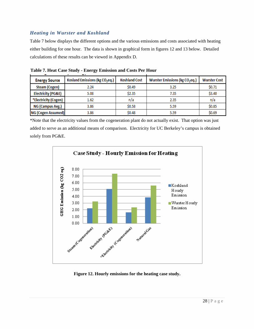
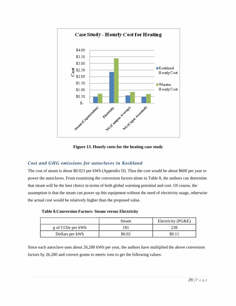
Heating in Wurster and Koshland Table 7 below displays the different options and the various emissions and costs associated with heating

either building for one hour. The data is shown in graphical form in figures 12 and 13 below. Detailed

calculations of these results can be viewed in Appendix D.

*Note that the electricity values from the cogeneration plant do not actually exist. That option was just

added to serve as an additional means of comparison. Electricity for UC Berkeley’s campus is obtained

solely from PG&E.

Figure 12. Hourly emissions for the heating case study.

Table 7. Heat Case Study - Energy Emission and Costs Per Hour

29 | P a g e

Figure 13. Hourly costs for the heating case study

Cost and GHG emissions for autoclaves in Koshland

The cost of steam is about $0.023 per kWh (Appendix D). Thus the cost would be about $600 per year to

power the autoclaves. From examining the conversion factors alone in Table 8, the authors can determine

that steam will be the best choice in terms of both global warming potential and cost. Of course, the

assumption is that the steam can power up this equipment without the need of electricity usage, otherwise

the actual cost would be relatively higher than the proposed value.

Table 8.Conversion Factors: Steam versus Electricity

Steam Electricity (PG&E) g of CO2e per kWh 181 238

Dollars per kWh $0.02 $0.11

Since each autoclave uses about 26,280 kWh per year, the authors have multiplied the above conversion

factors by 26,280 and convert grams to metric tons to get the following values:

30 | P a g e

Table 9. Powering a single autoclave in Koshland Hall in one year

Steam Electricity (PG&E) Global Warming Potential

(metric tons of CO2e) 4.8 per autoclave per year 6.3 per autoclave per year

Cost $600 per autoclave per year $2890 per autoclave per year

So as can be seen from Table 8, the conversion factors for steam are smaller than that for electricity,

indicating that steam would produce less grams of CO2e per kWh, and it would also cost less per kWh.

For powering a single autoclave in one year, UC Berkeley would not benefit by switching to electricity.

In fact, it would produce about 1.5 more metric tons of CO2e by switching to PG&E. As for cost, the

campus would spend at least $2290 more. Thus, Koshland Hall should continue using steam for powering

its twelve autoclaves as opposed to utilizing electricity.

SENSITIVITY ANALYSIS

To address some of the uncertainty associated with calculated GHG emission due to steam production,

several variable elements were adjusted around the anchored value to see how great the difference would

be under different assumption. The initial sensitivity analysis is done by changing the percentage of total

energy converted to steam (relative to electricity). The percentage of total energy that becomes steam is

calculated based on the total steam consumption in campus and the total natural gas burned on the plant.

However, this percentage calculation is not very reliable. For example, the steam enthalpy is assumed to

be a fixed value when used to convert pounds of steam the campus consumed into total energy in steam.

Steam enthalpy is a number that varies with pressure and temperature, so the authors expect the calculated

steam energy to be different from the actual value. Since the percentage of total energy that converts into

usable steam is critical in determining the campus steam GHG emission, the sensitivity analysis aims to

see how the variation in the calculated percentage affects the emission.

Here, the authors assume that steam energy ranges from 50% to 65% of the total energy generated. The

total steam emission is calculated based on the percentage, in addition to the 2008 protocol emission

factor. For example, if the percentage of total energy going into steam is 50%, the emission factor for that

amount of steam is 50% of the 54.3 kg CO2/MMBtu, which is 27.2 kg CO2/MMBtu. In other words, for

one MMBtu of energy generated, 27.2 kilograms of CO2 emissions would be tagged as emission

associated with steam production. Therefore, the emission factor becomes smaller with smaller

31 | P a g e

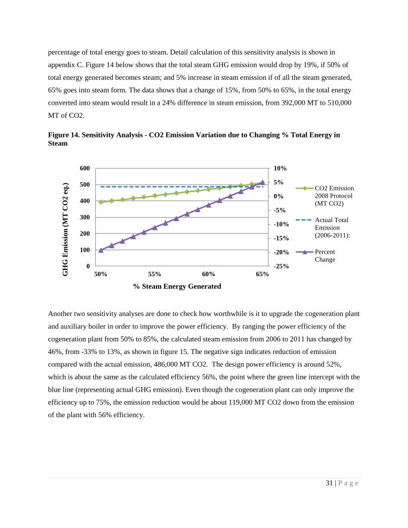
percentage of total energy goes to steam. Detail calculation of this sensitivity analysis is shown in

appendix C. Figure 14 below shows that the total steam GHG emission would drop by 19%, if 50% of

total energy generated becomes steam; and 5% increase in steam emission if of all the steam generated,

65% goes into steam form. The data shows that a change of 15%, from 50% to 65%, in the total energy

converted into steam would result in a 24% difference in steam emission, from 392,000 MT to 510,000

MT of CO2.

Figure 14. Sensitivity Analysis - CO2 Emission Variation due to Changing % Total Energy in Steam

Another two sensitivity analyses are done to check how worthwhile is it to upgrade the cogeneration plant

and auxiliary boiler in order to improve the power efficiency. By ranging the power efficiency of the

cogeneration plant from 50% to 85%, the calculated steam emission from 2006 to 2011 has changed by

46%, from -33% to 13%, as shown in figure 15. The negative sign indicates reduction of emission

compared with the actual emission, 486,000 MT CO2. The design power efficiency is around 52%,

which is about the same as the calculated efficiency 56%, the point where the green line intercept with the

blue line (representing actual GHG emission). Even though the cogeneration plant can only improve the

efficiency up to 75%, the emission reduction would be about 119,000 MT CO2 down from the emission

of the plant with 56% efficiency.

-25%

-20%

-15%

-10%

-5%

0%

5%

10%

0

100

200

300

400

500

600

50% 55% 60% 65%GH

G E

mis

sion

(MT

CO

2 eq

.)

% Steam Energy Generated

CO2 Emission2008 Protocol(MT CO2)

Actual TotalEmission(2006-2011):

PercentChange

32 | P a g e

Figure 15. Sensitivity Analysis - CO2 Emission Variation due to Changing Cogeneration Plant Power Efficiency

By changing the power efficiency of auxiliary boiler from 65% to 95%, variation of steam emission is

estimated. The assumed efficiency of the auxiliary boiler is 75%. As shown in figure below, even if the

auxiliary boiler is upgraded from 75% to 95%, the reduction of steam emission will be only 1.5%,

equivalent to 7,100 MT CO2. Based on the previous two sensitivity analyses, the authors can give some

suggestion and recommendation for the power plant later in the report.

Figure 16. Sensitivity Analysis - CO2 Emission Variation due to Changing Auxiliary Boiler Efficiency

-40%

-30%

-20%

-10%

0%

10%

20%

0

100,000

200,000

300,000

400,000

500,000

600,000

50% 55% 60% 65% 70% 75% 80% 85%GH

G E

mis

sion

(MT

CO

2 eq

.)

Cogenerataion Plant Power Efficiency

Result GHGEmission (MTCO2)

Actual GHGEmission(2006-2011)(MTCO2)PercentChange

-2%

-2%

-1%

-1%

0%

1%

1%

2%

472,000

477,000

482,000

487,000

492,000

497,000

65% 70% 75% 80% 85% 90% 95%

GH

G E

mis

sion

(MT

CO

2 eq

.)

Auxiliary Boiler Efficiency

Result GHGEmission(MT CO2)

Actual GHGEmission(2006-2011)(MTCO2)PercentChange

33 | P a g e

UNCERTAINTY ASSESSMENT AND MANAGEMENT

The data quality assessment takes into account the amount of uncertainty related to the data used in this

analysis. The quality of the data was evaluated using a multi-dimensional estimation framework based on

how, when, and where from the data is received. The score of 1 represents the data with highest certainty.

The majority of data comes from reliable sources (cogeneration managers, campus project, etc.), but some

data comes from educated assumptions (utility specification, system performance, etc,), which can be less

than desirable.

Table 10. Uncertainty Level of the Information

acquisition method

independence of data supplier

representativeness data age

geographical correlation

technological correlation

Cogeneration Production 3 1 1 1 1 1

Emission Reporting 1 3 1 2 1 1

Building Consumption 2 3 1 1 2 2

Lab Equipment

Specification 4 2 2 2 1 1

Maximum Quality 1 1 1 1 1 1

Minimum Quality 5 5 5 5 5 5

Some of the data had a rating of 3, indicating some assumption was placed in the data in order for them to

be presentable. Both the production and consumption of steam are metered values of how much passed

through the steam meter. This does not account for the loss steam may face after having been processed

or otherwise wasted within the building. While the steam may be transferred to the building, there is

currently no real quantifiable way to track how much is lost in each part of the building. The reason is that

the steam is considered wasted if the occupants do not “feel” the desired heat. One of the common

practices to alleviate this problem is to upsize steam output (delivering more than what is necessary so

enough can reach the users) at the cost of more consumption, which is not a desirable practice for long

term GHG mitigation. Based on differences in site conditions, applying Spath & Mann’s LCA estimation

34 | P a g e

into our cogeneration plant may also raise uncertainty, since there are additional factors other than scale

of the plant and production rate that determines the total GHG emission.

In the case of cogeneration/auxiliary boiler emissions, different protocols were used to estimate the

emission amount. However, in both GHG models, there was assumption of specific emission factors, as

well the efficiency for energy conversion in auxiliary boiler. While the authors have taken PG&E’s

proposed emission rate (in lbs CO2e/kWh) for comparison, the rate can still vary by time of day, year, and

with seasonal variations in weather. With different consumption patterns over different seasons, the

emission rate from each period of the year would need to be weighted accordingly when evaluating the

average rate. According to PG&E, the average rate has been independently certified by the California

Climate Action Registry, making the rate more trustworthy. How the certification was done, though, was

left out in both sources. As for natural gas emissions rate, PG&E’s estimate was directly taken from the

California Public Utility Commission.

In terms of efficiency, it would be difficult for a facility to maintain the same efficiency for a long period

of time without periodic maintenance. Based on previous discussion, the pipes in Wurster Hall need to be

lubricated periodically in order to prevent decreases in efficiency (E. Perszyk, personal communication,

November 27, 2012). The same case may apply to the cogeneration system as well given the period of

time it runs before maintenance. While the ongoing campus project suggested the efficiency of heat

conversion is assumed to be 75%, the authors would like to know the scientific reason behind it as well.

One of the challenges in the analysis was to quantify the actual amount of consumption done by lab

equipment such as the autoclave. Unlike each individual building, where the metered steam usages are

available, the steam usage for individual equipment cannot be as easily quantified. Unfortunately, the

authors were not able to get the equipment specifications directly from the building managers, so

assumptions were made on the specifications of autoclaves based on the best available data from

equipment manufacturing sites, several of which are from international companies. Likely, the

information provided was not the same as the actual steam consumption by the equipment at the Berkeley

campus, but again, the data on steam usage is relatively limited compared to electricity power usage.

Despite the uncertainty associated with our analysis, the authors were able to piece information from

different sources together in order to offer a more accurate representation of steam GHG emissions on the

campus. In addressing uncertainty associated with efficiency in the cogeneration plant, the authors have

recalculated efficiency based on natural gas input and the usable energy outputs. With more data, the

authors were able to have more data robustness, using design efficiency as desired. In addition, sensitivity

analysis on plant efficiency can be done to visualize the magnitude of GHG reduction.

35 | P a g e

INTERPRETATION AND DISCUSSION OF RESULTS

Possible Protocol/Assumption Improvements The protocols only take carbon dioxide, methane, and nitrous oxide into account when converting natural

gas into greenhouse gas emissions. Greenhouse gases, however, also include other gases such as water

vapor and ozone. Stream production should be incorporated into the calculations of greenhouse gas

emissions. Furthermore, the other greenhouse gases should be accounted for either as a general error

adjustment or as specific gases with their emission factors.

The protocols also assume that natural gas is not lost during transportation. In other words, 100% of the

natural gas used by the facilities is 100% of the natural gas produced. In actuality, a small amount of

steam and natural gas may be lost not only in transportation, but also through the efficiency of the

systems using the steam or natural gas. Thus, some transportation some transportation losses should be

assumed. If the new estimation is an overestimate, it would be better than the current protocols which

give underestimations. This is because overestimations of greenhouse gas emissions would encourage

reductions in usage. At the same time, an underestimation for 1990 levels would be more beneficial

because then the goal is harder to attain.

Emissions Protocol and LCA of Cogeneration Plant and Auxiliary Boilers The 2006 and 2008 protocols from the General Reporting Protocol are similar, so the conversion from

indirect emissions of natural gas to Global Warming Potential (pounds of CO2e) was done correctly in the

campus report. When looking at the two protocols, the basic outcome is the same. The 2008 protocol has

a slightly larger emissions factor for carbon dioxide, 53.06 kg/MMBtu versus 52.78 kg/MMBtu, and a

slightly smaller methane emissions factor 0.001 kg/MMBtu versus 0.0059 kg/MMBtu. These are the only

differences, and that change does not affect much. The total steam emissions from the cogeneration plant

changed from 180 g CO2 eq. per kWh produced in the 2006 protocol to 181 g CO2 eq. per kWh produced

in the 2008 protocol, which is an unnoticeable change. Therefore, UC Berkeley did not miss much of the

emissions by using the 2006 protocol.

The LCA takes into account more emissions than regular emissions calculations, like the 2006 and 2008

protocols. As was seen in the LCA results earlier, only about 75% of the total life-cycle emissions of a

cogeneration plant are associated with operating the plant. Nearly a quarter of the emissions come from

natural gas extraction and distribution, and that figure was shown to possibly increase based on the

percentage of fugitive emissions from the natural gas. Therefore, UC Berkeley would be missing large

amounts of emissions by ignoring the whole life of the plant. The emissions protocol calculates emissions

36 | P a g e

to be 181 g CO2 eq. per kWh produced, and the LCA sees it at 255-325 g CO2 eq. per kWh produced. The

gap between the two values makes a large difference when it is accumulated over years of emissions. Of

course, if steam GHG emission is to be compared with other energy types’ (such as renewable energy), it

would be necessarily to consider their LCA emission as well, which would require further studies into

different processing done in their life cycles.

For the auxiliary boilers it is much the same story. The LCA value of 302 g CO2 eq. per kWh of steam

produced factors in much more emissions than what is currently being assumed by the university. That

being said, the authors encourage the university to take a life-cycle outlook on emissions for the sake of

comprehensiveness.

The basis of this study was to clarify UC Berkeley’s association with GHG emissions for steam

generation. Yet, without proper analyses, the university is not taking responsibility for a substantial

portion of its emissions - the cogeneration plant is in the same boat. Unfortunately, in today’s time, no

organization would be taking responsibility of those ‘overlooked’ emissions that are prevalent in an LCA

analysis. Therefore, both the university and the cogeneration plant, in this case, should take responsibility

of the ‘total’ LCA emissions so that both parties can take action to reduce those emissions.

Koshland and Wurster Steam Comparison Between Koshland and Wurster Halls, Koshland Hall is the newer and smaller building but it uses

substantially more steam than Wurster Hall. The difference is likely attributable to the fact that Koshland

Hall is a bioscience building where laboratories are regularly conducted whereas Wurster Hall is a mixed

use building used for lectures, discussions, studios, a lab, and a cafe. Although Wurster Hall was

renovated in 2002, it was mainly seismically renovated, so it still uses the same pipes it was built with in

1964. Thus, the authors can only reasonably attribute a small portion, if any, of the energy efficiency to

renovation. Most of the difference will be due to the labs

because the lab buildings must heat and pressurize environments for sterilization purposes at all times of

the day.

The huge difference in steam consumption between the two buildings indicates variability in the buildings

in terms of steam usage, which signifies that certain alternatives may work for one building and not for

others. Therefore, synthesizing a solution that would benefit a large portion of the campus is a challenge.

Another challenge is the determination of alternatives for the steam being used on the campus, but

through some evaluation, the authors determined that for powering the lab equipment and heating the

buildings, steam shows the strongest competitive edge.

37 | P a g e

Case Study: Looking Into Heating From looking at figure 12 and figure 13, it can be seen that steam poses the best option for heating, both

in terms of emissions and costs. The natural gas assumed rate for the cogeneration plant is slightly more

competitive in terms of cost, and that is due to the large quantity of natural gas that would be

purchased. The emissions associated with that option are a lot higher than steam, however. As well, if

the UC Berkeley campus received electricity from the cogeneration plant, the emissions values would be

a lot lower - this is because the plant shares electricity emissions with the generation of steam. Yet, the

cost is uncertain and it would likely be similarly priced to the electricity that is bought from the PG&E

mix.

Nevertheless, based off this simple analysis of looking at heating a building for an hour on an average

cold day in Berkeley, California, it is quite evident that steam yields the most promising option as the

source of energy to heat the buildings. In that sense, fewer additional costs are associated with this

alternative because most of the infrastructure associated with steam is already in place.

Through the heating case study, it was clearly shown that steam plays the best role in terms of

emissions. Over the course of an hour, 2.24 kg CO2 eq. was emitted for Koshland Hall using steam,

compared to the 5.08 kg CO2 eq. that was observed for the PG&E mix, and the 3.86 kg CO2 eq. that was

emitted for natural gas. The same relationship was observed in the Wurster Hall heating, and the bottom

line here is that steam is the best from an environmental perspective. The electricity generation from the

cogeneration plant is not current option for UC Berkeley, but from the emissions plot in figure 12, it can

be seen that it would have lower emissions than steam. Essentially, the sum of the steam bar from the

figure and the cogen electricity bar from the figure are the total emissions of the cogeneration plant. It

can be observed, however, that obtaining electricity from the cogeneration plant is much cleaner than

steam, and the reason for this was explained earlier in the report (steam is associated with a higher

percentage of the overall emissions of the cogeneration plant, because emissions are determined based on

energy content of the products produced by the plant). Nonetheless, this electricity is not an option, and

steam poses the best alternative.

Looking at the cost comparison for this case study, steam demonstrated the lowest cost at $0.49 for one

hour of heating in Koshland Hall. The gap between steam and natural gas, in terms of cost, was lower

than that of the emissions, with natural gas costing $0.58 for that same hour of heating in Koshland

Hall. Electricity was the most expensive here at $2.35 per hour of heating, and the relationships between

energy costs is consistent in Wurster Hall (as all of this is based on floor area). There was a postulated

value for the price of natural gas that the cogeneration plant buys, and this is calculated in detail in

38 | P a g e

Appendix D. In any case, if the cogeneration assumed rate is used for natural gas, the cost to heat

Koshland Hall for an hour is marginally cheaper than steam at $0.48. Once again, this is not an option, so

steam is the best in terms of cost as well.

However, it is important to note that these conclusions are based on the assumptions that the pipes and

other equipment used to heat the building are functioning properly. If there are leaks in the pipes or other

issues, using steam may be less efficient than electricity. For example, in Wurster Halls, the pipes are

very old and inefficient. In fact, the pipes are the original pipes from 1964 and cannot be replaced since

they are original and out of production. Although some efforts can be made to improve the heating

process, many individuals are dissatisfied with the temperatures in Wurster Hall and have brought in

space heaters to use. These space heaters use electricity, and they are operating when the steam heating is

also in operation. In other words, both steam and electricity are in use at the same time (E. Perszyk,

personal communication, November 27, 2012). Therefore, through this small heating case study, it is

clear that steam is not only more environmentally friendly, but it is also less costly than its competing

alternatives. Yet, if the steam is not operating at ideal levels, emissions and costs can be reduced to just

use the alternative of electricity.

Case Study: Looking Into Labs – Autoclaves From looking at the conversion factors for steam and electricity (from PG&E), steam again showed to be

a better option, both emitting less CO2e per kWh (181 g per kWh compared to 238 g per kWh) and also

costing substantially less ($0.023 per kWh instead of $0.11 per kWh). When considering the large

amounts of kWh used by the lab equipment, the difference between using steam and using electricity

becomes even greater. Assuming the same efficiencies between steam and electricity, using steam to run

the lab equipment would be the better choice.

For each autoclave, about 26,280 kWh are used per year. This equates to about 2190 kWh per month per

autoclave. By using the conversion factors previously determined (0.0034 MMBtu/kWh and 1.193

MMBtu/kLb), the pounds of steam used by each autoclave per month is calculated to be about 6240.

Since Koshland Hall has twelve autoclaves, the total pounds of steam consumed by the twelve autoclaves

are about 75,000 pounds per month.

Heating Koshland Hall consumes about 21.35 kW (Appendix E) which is about 4329 kWh per month.

This is powered by about 12,000 pounds of steam per month. The sum of the steam consumed for heating

and the steam consumed by the autoclaves is about 87,000 pounds. Without considering the efficiency

associated with energy conversion in the lab equipments, the estimate for steam consumption by

autoclaves contradicts with the hypothesis that lab equipments consumed the majority of steam in

39 | P a g e

Koshland. Recall that from July 2011 to June 2012, about 2 to 4 million pounds of steam were fed to

Koshland Hall per month (Figure 9). Based on that logistics, the autoclaves account for at most 4.5% of

the building’s steam usage. The low estimate may indicate that either the authors failed to include

significant factors, such as appropriate consumption amount per unit, or the amounts of steam fed to the

buildings are truly greater than the actual amounts used.

Sensitivity analysis could have been done to address issues with uncertainty in regards to Koshland’s

equipment steam consumption, but the authors did not find enough credible information pertaining to

steam power consumption from manufacturing sites. If more reference values for power consumptions

were available, it would be possible to interpolate power consumption to be used in sensitivity analysis,

comparing varying power consumption of steam in relation to percentage lab uses in total Koshland steam

consumption.

CONSTRAINTS

Being this was an analysis of a campus issue, the authors were required to work with UC Berkeley and

obtain data and information from the university. There was a great deal of complication, however,

associated with obtaining the necessary information required for the analysis in this research project. Part

of this complication was due to not being able to get a hold of certain people in the campus, regardless of

the number of efforts made, and this issue persisted throughout the entire duration of the research

project. Whether the contact was desired for actual data, for specific building or infrastructure

information, or just general information, there was great complication in obtaining what the authors

needed to conduct a proper analysis.

UC Berkeley would like to use the results presented in this report, however, if the community on campus

is not willing to assist the authors in this analysis, this adds a great constraint to the research and places a

barrier in the depth of analysis that can be performed. The authors are aware that the campus community

is comprised of busy working people who are taking time to do their own jobs. Yet, the authors feel that

over the course of a semester, some free time should surely exist. Nevertheless, this is the case for the

analysis in this report.

With that being said, the authors are extremely disappointed that the research in this report was not

allowed to develop the way it should have, and even more disappointed that the campus community was

not entirely willing to assist this research. In sum, the authors have done extensive work to go around the

constraints that existed in this project, and they feel that they have done a great job finalizing this detailed

40 | P a g e

report, despite the constraints. The authors, however, want to make it clear that this report did have the

potential to be deeper if the constraints did not exist in the first place.

In addition, the authors would like to thank Gilbert Escobar and Kira Stoll for being the two main sources

of information from campus, with a select few of others helping out in lesser amounts elsewhere.

RECOMMENDATIONS

Based on this analysis of steam, there are strong signs that indicate steam should be continued to be used

for its current purposes - HVAC, domestic hot water and equipment use. With that being said, there is a

lot of financial benefit to this. Major improvements or alterations to the system are not required for the

campus as a result, because the campus has already been setup to use steam for the uses mentioned

above. This obviously lessens, or even eliminates, the costs that would be associated with changing the

form of energy that would be used for HVAC, DHW or equipment use.

Since the big picture idea is to keep the steam, and the steam system is already in place, improving the

current system is the only route to lowering the GHG emissions that are associated with the steam. The

subsequent sections will elaborate on suggestions that the campus can uptake in improving the steam

system. Some of the suggestions are associated with large capital costs, and the authors are aware that

UC Berkeley is currently in a financial crisis with large budget cuts. For the purpose of completeness,

however, the authors have posed a variety of suggestions with the intent that UC Berkeley may accept

some of the recommendations, and that the suggestions will allow the campus community to begin

thinking together about other solutions.

General Suggestions Steam is purchased based on campus demand and is governed by the UC Berkeley campus’ necessity for

it. With that thought in mind, the simple solution to mitigating emissions is to limit the amount of steam

that is drawn into the UC Berkeley campus. In order to accomplish this task, however, there are several

approaches UC Berkeley can take. The main idea is to lower the demand for steam, and that way less will

be produced. An inherent benefit to lowering the demand will be the lessened use of the auxiliary

boilers. Although, these boilers do not add much emission to the overall steam emissions figure, the

equipment is much less efficient at generating steam than the cogeneration plant, and it is not as clean

either.

41 | P a g e

Improving the end-user efficiency in the buildings themselves will aid in the decreasing of demand. An

example of this would be to improve the heating or lab equipment to be more efficient at using the steam

that those pieces of equipment consume. Wurster Hall is a building that is fairly inefficient, mainly due to

its age. Needless to say, an improvement on the buildings steam use efficiency would lower the demand

of steam consumed by that building, and thus emissions overall. Improving the steam plumbing in

Wurster Hall would greatly improve the system efficiency, for example, and it could be accompanied by a

more impenetrable building envelope, or insulation. The main idea is that there are many options that

would lead to bettering the efficiency at the building end of the system. As well, enhancements to the

cogeneration plant itself would also aid in lowering the GHG emissions, and this is further discussed in

the following section: Cogeneration Plant Efficiency Suggestions.

A final general suggestion that the authors had was for the UC Berkeley campus to generate a campus-

wide utility database with utility ratings. In their study, the authors had a large amount of difficulty

analyzing Wurster and Koshland Halls. A lot of this struggle was due to the lack of complete information

regarding the utilities that are within the buildings themselves. Overview of what the building uses to

heat or cool inner environment was clear and obvious (e.g. 100% re-circulated air is used to ventilate

Wurster hall). Yet, the type of heating equipment, its size and utility consumption are examples of

uncertainty that prevailed in the analysis. For this reason, the authors believe that the campus would

benefit greatly from generating a database that compiles detailed information about utilities, and the dates

they were installed, especially for the recently built buildings. It would make updating equipment and

analyzing utility efficiencies much less chaotic and much more accurate.

Cogeneration Plant Efficiency Suggestions

Although the cogeneration plant is not owned by the UC Berkeley campus, the authors would like to

suggest possible improvements, both for comprehensiveness and for the sake that there may be a

possibility for the campus to have some influences on the decisions the owner of the plant makes (which

are discussed in the subsequent section). Here are some suggestions.

In the Berkeley cogeneration plant, considering the total plant fuel heat input and the plant output both in

electrical energy plus heat in the export steam less the heat in the return condensate result in an overall

efficiency of about 52%. However, this efficiency will vary with operating conditions (UC Berkeley

Facilities Services, 2003). As mention above, the Berkeley cogeneration plant was built in 1980s, so there

is efficiency loss due to depreciation of the mechanical equipments over time, such as turbines. Since the

42 | P a g e

Cogeneration plant is using the Natural Gas Combined Cycle technology; gas turbine and steam turbine

are both needed to generate electricity and steam at the same time. According to a report on Power

Magazine, to keep any plant on-line and profitable requires continuous investment; and it only seems

reasonable to invest in area where the return on investment will be biggest, such as upgrading a steam

turbine (Peltier, 2006). A case study was done on a turbine upgrading project at Dubai. GE modified

turbines in a 30-year-old cogeneration plant at Dubai Aluminum with tighter seals, higher firing

temperature and improved airflow. The changes increased power output by 13% (Studebaker 2010).

Other mechanical parts, such as heat pumps and heat recovery system generator, are also possible to

improve overall efficiency by retrofit or upgrade. Besides retrofit of the old plant, regular maintenance

should be done as well. A performance monitoring study was done in a cogeneration plant at Italy,

showing that operating efficiency was recovered and availability increased after maintenance procedure

(Piscitelli 2010). Therefore, maintenance should be regularly done to make sure the cogeneration plant

runs at its best possible efficiency.

As UC Berkeley owns the three auxiliary boilers, authors have some recommendation for efficiency

improvement for the boilers. According to a report from the Energy Observer, the minimum allowed

rating for a gas-fueled steam boiler is 75%, which is exactly the same as the assumed power efficiency of

auxiliary boilers. Some upgrades or retrofits can be done to make sure the auxiliary boiler efficiency will

not drop below the minimum allowed rating. There are two major ways to improve efficiency of boilers.

One is to replace the existing boilers; the other is to retrofit the inefficient boilers. By replacing the boiler,

the newer system can have efficiency up to 97%. If replacing the boiler is not cost-effective or financially

feasible, a number of retrofits are possible. Adding a vent damper prevents chimney losses by closing off

a boiler’s vent when the boiler isn’t firing is the most beneficial option for large steam boilers. Other

options include using intermittent ignition devices as opposed to pilot light burning continuously, derating

the gas burner if it is oversized, or using modulating aquastats to control the temperature in the boiler

(The Energy Observer, 2009). However, the end problem comes to if it is worthwhile to do the retrofit or

upgrade. According to the result from sensitivity analysis, the GHG emission will be only 1% less than

the actual emission even though the efficiency of the boiler goes up to 95%. This is because the campus

only uses the boiler when the demand of the steam is too high. Economically speaking, keeping the

existing boiler as how they are now is recommended, so if a newer cogeneration plant with higher

capacity is available in future to support the campus steam usage, the campus may choose to

decommission the boilers.

43 | P a g e

Year 2017 In the year 2017, the 30-year contract between UC Berkeley and the third party-owned cogeneration plant

will expire. That being the case, some action has to be taken to formulate a solution for the campus. The

authors suggest the campus to keep the plant running, first off. Beyond that, there are a couple options

the authors would like to recommend to the campus.

The first option is to renew the contract, at least for a short period of time. There currently are no

thoughts about to do when the contract expires and this option will allow the campus to buy some time to

come up with other solutions as well. In addition, UC Berkeley is not fit to run a power plant, and that

idea is strongly discouraged.

A second option would be to have the campus finance the cogeneration plant in updating and continue

with a contract with the plant. By updating the plant with more efficient equipment, both the

cogeneration plant and the campus will be associated with lesser emissions. As well, the funding that the

campus would provide to the cogeneration plant could also allow the campus to take a partial stake in

ownership of the plant, but not in such a way that the campus would be responsible for operating and

maintaining the plant - the funding would just be an encouragement to help upgrade the plant equipment.

44 | P a g e

CONCLUSIONS

In conclusion, the analysis done for this report was limited by certain constraints existent in the UC

Berkeley community, and the analysis did not develop to its desired potential. The campus, however, can

still take action to improve the current steam system. Regardless of the approach that UC Berkeley takes,

the authors would strongly encourage the campus to keep the cogeneration plant as a steam provider, and

beyond that, keep using steam the way it does, but improve on efficiencies to limit the actual amount of

steam consumed. Of course, many of the effective solutions are associated with a cost, and some of those

costs can be large. UC Berkeley is a public university and in the current economy it is clear that the

school does not have excess funds lying around. Improvements, however, do not have to be large,

because every change will be helpful. Larger changes have a greater impact, but are not always

feasible. Even the sharing of information and allowing the community at UC Berkeley to be more aware

of the issue, and what they can do to help will aid in the solution.

Reducing emissions associated with steam is not a one-person task, and it will not happen

overnight. Taking the initial steps to begin improving the system, and beginning to work together will go

a long way. Be it improvements in efficiencies at the cogeneration plant itself, or in the buildings that use

the steam, or spreading the word, the enhancement of any part of the system will aid in the mitigation of

GHG emissions in the end.

45 | P a g e

REFERENCES Ahmed, F. (2007). UC Berkeley Climate Action Partnership: Feasibility Study 2006-2007 Final

Report. Berkeley, CA: UC Berkeley Climate Action Partnership. Retrieved December 3, 2012, from http://sustainability.berkeley.edu/calcap/docs/CalCAP%20Report%20FINAL%202007.pdf.

Althouse, A.D., Turnquist, C.H., Bracciano, A.F. (1996). Modern Refrigeration and Air Conditioning. Tinley Park, IL: The Goodheart-Willcox Company, Inc.

Bolland, O. (1993). Assessment of Cogeneration Systems Performance. NTNU(Norwegian University), Thermal Energy & Hydropower. Retrieved October 12, 2012, from http://www.ivt.ntnu.no/ept/fag/ep8103/innhold/cogen_as.pdf.

California Energy Commission. (2010). Watson Cogeneration Steam and Electric Reliability - Preliminary Staff Assessment (Docket No. 09-AFC-1). Sacramento, CA: California Energy Commission. Retrieved October 14, 2012, from http://www.energy.ca.gov/2010publications/CEC-700-2010-020/CEC-700-2010-020-PSA.PDF.

Cockrell, C. (2003) ‘Wurster Redux’ Celebrates CED Milestones. UC Berkeley News. Retrieved November 14, 2012, from http://www.berkeley.edu/news/berkeleyan/2003/10/01_wrstr.shtml.

Duffy, G.K. (2010). Steam Loss In Miami University Piping System, Miami University, Oxford, OH. Retreived October 11, 2012, from http://www.aashe.org/files/resources/student-research/2009/449_final_report.pdf.

Gas Cum Electric Autoclaves. Narang Medical Limited. - AU715-35. Received December 2, 2012, from http://www.narang.com/autoclave-sterilizers/gas-cum-electric-autoclaves/AU715-35.php.

Gas Rate Finder. Pacific Gas and Electric Company. (December 2012). Retrieved November 27, 2012, from http://www.pge.com/tariffs/GRF1212.pdf.

General Reporting Protocol. The Climate Registry. Version 1.1. (May 2008). Retrieved October 14, 2012, from http://www.theclimateregistry.org/downloads/GRP.pdf.

How Many BTUs to Heat 1 Square Foot? eHow – Home. (2012). Retrieved November 27, 2012, from http://www.ehow.com/way_6148246_many-btus-heat-square-foot_.html.

Lipman, T. (2011). University of California - Berkeley: 25 MW CHP System: Project Profile. Berkeley, CA: Pacific Region CHP Application Center. Retrieved December 3, 2012, from http://www.pacificcleanenergy.org/PROJECTPROFILES/pdf/UC_Berkeley.pdf.

http://www.theclimateregistry.org/downloads/GRP.pdf

46 | P a g e

Monthly Temperatures. The Weather Channel. (2012). Retrieved November 27, 2012, from http://www.weather.com/weather/wxclimatology/monthly/graph/94720.

National Energy Technology Laboratory. (2010). Life Cycle Analysis: Power Studies Compilation Report (DOE/NETL-2010/1419). Washington, D.C.: US Department of Energy. Retrieved December 3, 2012, from http://www.netl.doe.gov/energy-analyses/pubs/PowerLCA_Comp_Rep.pdf.

New York University (2010). NYU Climate Action Plan. Retrieved October 16, 2012, from http://www.nyu.edu/sustainability/pdf/capreport10.pdf.

Osman, A., Ries, R. (2006), Optimization For Cogeneration Systems in Buildings Based on Life Cycle Assessment. Journal of Information and Technology in Construction. 20(11), pp. 269-284.

Osman, A. Ries, R. (2007). Life Cycle Assessment of Electrical and Thermal Systems for Commercial Buildings. International Journal of LCA. 12(5), pp.308-316.

Pacca, S., and Horvath, A. (2002). Greenhouse Gas Emissions from Building and Operating Electric Power Plants in the Upper Colorado River Basin. Environmental Science & Technology, ACS, 36(14), pp. 3194-3200.

Peltier, Robert (2006). Steam Turbine Upgrading: Low-hanging Fruit. Power Magazine, Vol. 150. No.3 April 2006, Digital Version. Retrieved November 27, 2012, from http://www.turbocare.com/turbocare/Articles/STUpgrade_Madgett.pdf.

PG&E Carbon Footprint Calculator Assumptions (2012). Retrieved December 2, 2012, from http://www.pge.com/about/environment/calculator/assumptions.shtml.

Piscitelli, Vincenzo (2010). Performance Monitoring To Increase Power Plant Efficiency. Cogeneration & On-Site Power Production, September - October 2010. Retrieved November 26, 2012, from http://www2.emersonprocess.com/siteadmincenter/PM%20Articles/COSPP0911_perfmonitor.pdf.

Stanford University (2011). Sustainable Stanford | Emissions Inventory. Retrieved October 16, 2012, from http://sustainablestanford.stanford.edu/emissions_inventory.

http://www.pge.com/about/environment/calculator/assumptions.shtml

http://www2.emersonprocess.com/siteadmincenter/PM%20Articles/COSPP0911_perfmonitor.pdf

47 | P a g e

Spath, P.L., Mann, M.K. (2000). Life Cycle Assessment of Natural Gas Combined-Cycle Power Generation System. National Renewable Energy Laboratory. Retrieved from October 12, 2012, from http://www.nrel.gov/docs/fy00osti/27715.pdf.

Studebaker, Paul (2010). Turbine retrofit ups efficiency 13%- Cogeneration of heat or steam and electric power can yield fuel efficiencies. Retrieved November 27, 2012, from http://www.plantservices.com/articles/2010/01TurbineRetrofit.html.

The Energy Observer (2009). Energy Information for the Facility Manager, Upgrade the Boiler! Quarterly Issue, March 2009. Retrieved November 26, 2012 from http://www.michigan.gov/documents/dleg/EO_03-09_271516_7.pdf.

Twu, Alfred (2005). Alfred Twu's Tour of UC Berkeley. Alfred Twu's OCF Page. UC Berkeley Open Computing Facility, Sept. 2005. Web. Retrieved December 3, 2012, from http://www.ocf.berkeley.edu/~atwu/firstcultural/berkeleyguide.html.

UC Berkeley FacilitiesLink. (2012). Wurster - Detailed Building Record. Berkeley, CA: UC Berkeley FacilitiesLink. Retrieved October 11, 2012, from https://berkeley .digicality .com/Buildings/Details/Def ault.htm?Bkey =277&Media=Printer.

UC Berkeley FacilitiesLink. (2012). Koshland - Detailed Building Record. Berkeley, CA: UC Berkeley FacilitiesLink. Retrieved October 11, 2012, from https://berkeley.digicality.com/Buildings/Details/Default.htm?Bkey=276.

UC Berkeley Facilities Services. (2003). Berkeley Cogeneration. Berkeley, CA: UC Berkeley Facilities Services.

Using Autoclave Safely. EH&S Fact Sheets. UC Office of Environment, Health & Safety (2011). Retrieved December 2, 2012, from http://ehs.berkeley.edu/pubs/154-factsheets.html.

World Energy Council. (2004). Comparisons of Energy Systems Using Life Cycle Assessment. London, United Kingdom: World Energy Council. Retrieved December 3, 2012, from http://www.worldenergy.org/documents/lca2.pdf.

Wurster Hall Redux. Studio Urbis. Retrieved November 14, 2012 from http://www.studiourbis.com/projects/wp.htm.

http://www.nrel.gov/docs/fy00osti/27715.pdf

http://www.plantservices.com/articles/2010/01TurbineRetrofit.html

http://www.michigan.gov/documents/dleg/EO_03-09_271516_7.pdf

http://www.ocf.berkeley.edu/~atwu/firstcultural/berkeleyguide.html

http://ehs.berkeley.edu/pubs/154-factsheets.html

A-1 | P a g e

Gas Burned_MMBtu Gas Burned_MMBtu Gas Burned_MMBtu

Total

Eletrical

Production

Steam

Production

(MMBtu)

Percent

Energy in

Steam

Steam

Production

(MMBtu)

Total Steam

consumption

(MMBtu)

Annual

Steam

Consumption

(Cogen + Aux Broiler) (Cogen Only) (Aux Only) MMBTU Cogen Only Aux Only (Cogen+Aux) (MMBtu)

Jan-06 2.31E+05 2.23E+05 7.89E+03 6.24E+04 9.80E+04 61% 5.92E+03 1.04E+05

1.00E+06

Feb-06 2.02E+05 1.96E+05 6.69E+03 5.57E+04 8.28E+04 60% 5.01E+03 8.79E+04

Mar-06 2.26E+05 1.96E+05 2.99E+04 5.40E+04 8.63E+04 62% 2.24E+04 1.09E+05

Apr-06 2.11E+05 2.05E+05 6.02E+03 5.78E+04 9.07E+04 61% 4.52E+03 9.52E+04

May-06 2.05E+05 2.05E+05 0.00E+00 6.16E+04 7.58E+04 55% 0.00E+00 7.58E+04

Jun-06 1.87E+05 1.86E+05 1.79E+03 5.75E+04 5.94E+04 51% 1.35E+03 6.08E+04

Jul-06 1.91E+05 1.88E+05 2.51E+03 5.82E+04 6.36E+04 52% 1.88E+03 6.54E+04

Aug-06 2.00E+05 1.99E+05 1.27E+03 6.00E+04 7.05E+04 54% 9.55E+02 7.15E+04

Sep-06 1.93E+05 1.92E+05 1.41E+03 5.81E+04 6.95E+04 54% 1.06E+03 7.05E+04

Oct-06 2.04E+05 2.04E+05 1.03E+02 6.10E+04 7.62E+04 56% 7.72E+01 7.62E+04

Nov-06 1.94E+05 1.83E+05 1.07E+04 5.40E+04 7.59E+04 58% 8.05E+03 8.39E+04

Dec-06 2.27E+05 2.18E+05 9.23E+03 6.29E+04 9.38E+04 60% 6.92E+03 1.01E+05

Jan-07 2.52E+05 2.33E+05 1.81E+04 6.48E+04 1.05E+05 62% 1.36E+04 1.19E+05

1.03E+06

Feb-07 2.12E+05 2.05E+05 7.28E+03 5.68E+04 9.10E+04 62% 5.46E+03 9.65E+04

Mar-07 2.16E+05 2.11E+05 5.61E+03 6.00E+04 8.72E+04 59% 4.21E+03 9.14E+04

Apr-07 1.90E+05 1.60E+05 2.95E+04 4.69E+04 6.11E+04 57% 2.22E+04 8.32E+04

May-07 2.11E+05 2.06E+05 4.86E+03 5.92E+04 7.98E+04 57% 3.65E+03 8.35E+04

Jun-07 1.93E+05 1.88E+05 5.61E+03 5.54E+04 7.04E+04 56% 4.21E+03 7.46E+04

Jul-07 2.00E+05 1.97E+05 2.64E+03 5.86E+04 6.98E+04 54% 1.98E+03 7.18E+04

Aug-07 2.05E+05 2.04E+05 8.58E+02 6.03E+04 7.41E+04 55% 6.43E+02 7.47E+04

Sep-07 1.93E+05 1.89E+05 3.90E+03 5.72E+04 6.72E+04 54% 2.93E+03 7.01E+04

Oct-07 2.11E+05 2.07E+05 3.95E+03 6.06E+04 7.58E+04 56% 2.96E+03 7.88E+04

Nov-07 1.89E+05 1.75E+05 1.40E+04 5.08E+04 7.17E+04 59% 1.05E+04 8.22E+04

Dec-07 2.27E+05 2.14E+05 1.29E+04 5.88E+04 9.64E+04 62% 9.64E+03 1.06E+05

Appendix A – UC Berkeley Monthly Steam Consumption 2006 -2011

A-2 | P a g e

DATE Gas Burned_MMBtu Gas Burned_MMBtu Gas Burned_MMBtu

Total

Eletrical

Production

Steam

Production

(MMBtu)

Percent

Energy in

Steam

Steam

Production

(MMBtu)

Total Steam

consumption

(MMBtu)

Annual

Steam

Consumption


Jan-08 2.50E+05 2.30E+05 1.98E+04 6.23E+04 1.03E+05 62% 1.49E+04 1.18E+05

1.05E+06

Feb-08 2.24E+05 2.12E+05 1.19E+04 5.75E+04 9.41E+04 62% 8.96E+03 1.03E+05

Mar-08 2.28E+05 2.25E+05 2.93E+03 6.24E+04 9.90E+04 61% 2.20E+03 1.01E+05

Apr-08 1.99E+05 1.80E+05 1.92E+04 5.08E+04 7.51E+04 60% 1.44E+04 8.95E+04

May-08 2.15E+05 2.14E+05 9.81E+02 6.36E+04 8.13E+04 56% 7.36E+02 8.20E+04

Jun-08 2.01E+05 1.99E+05 1.96E+03 6.05E+04 7.30E+04 55% 1.47E+03 7.44E+04

Jul-08 2.01E+05 2.00E+05 1.59E+03 6.15E+04 7.07E+04 53% 1.19E+03 7.19E+04

Aug-08 2.03E+05 1.98E+05 4.46E+03 6.03E+04 7.32E+04 55% 3.34E+03 7.66E+04

Sep-08 1.76E+05 1.62E+05 1.38E+04 5.00E+04 5.74E+04 53% 1.04E+04 6.77E+04

Oct-08 1.86E+05 1.72E+05 1.43E+04 5.23E+04 5.91E+04 53% 1.07E+04 6.98E+04

Nov-08 2.02E+05 1.98E+05 3.81E+03 5.84E+04 8.02E+04 58% 2.86E+03 8.31E+04

Dec-08 2.41E+05 2.28E+05 1.34E+04 6.46E+04 1.01E+05 61% 1.00E+04 1.11E+05

Jan-09 2.25E+05 2.17E+05 8.52E+03 6.25E+04 8.94E+04 59% 6.39E+03 9.57E+04

1.01E+06

Feb-09 2.12E+05 2.02E+05 1.02E+04 5.71E+04 8.90E+04 61% 7.68E+03 9.66E+04

Mar-09 2.31E+05 2.25E+05 5.69E+03 6.46E+04 9.68E+04 60% 4.27E+03 1.01E+05

Apr-09 2.00E+05 1.87E+05 1.33E+04 5.49E+04 7.54E+04 58% 9.94E+03 8.53E+04

May-09 2.05E+05 1.99E+05 6.90E+03 5.91E+04 7.48E+04 56% 5.18E+03 8.00E+04

Jun-09 2.04E+05 2.03E+05 1.48E+03 6.00E+04 7.55E+04 56% 1.11E+03 7.66E+04

Jul-09 1.91E+05 1.77E+05 1.39E+04 5.28E+04 6.34E+04 55% 1.04E+04 7.38E+04

Aug-09 2.07E+05 2.05E+05 1.51E+03 6.02E+04 7.51E+04 56% 1.13E+03 7.62E+04

Sep-09 1.94E+05 1.94E+05 0.00E+00 5.87E+04 6.75E+04 53% 0.00E+00 6.75E+04

Oct-09 2.07E+05 2.04E+05 3.03E+03 6.01E+04 7.76E+04 56% 2.27E+03 7.99E+04

Nov-09 1.44E+05 8.67E+04 5.74E+04 2.46E+04 2.94E+04 54% 4.31E+04 7.25E+04

Dec-09 2.24E+05 2.17E+05 7.62E+03 5.44E+04 1.02E+05 65% 5.72E+03 1.08E+05

A-3 | P a g e

DATE Gas Burned_MMBtu Gas Burned_MMBtu Gas Burned_MMBtu

Total

Eletrical

Production

Steam

Production

(MMBtu)

Percent

Energy in

Steam

Steam

Production

(MMBtu)

Total Steam

consumption

(MMBtu)

Annual

Steam

Consumption


Jan-10 2.23E+05 2.11E+05 1.23E+04 5.69E+04 9.51E+04 63% 9.26E+03 1.04E+05

1.04E+06

Feb-10 2.04E+05 2.01E+05 2.90E+03 5.65E+04 9.18E+04 62% 2.17E+03 9.40E+04

Mar-10 2.21E+05 2.15E+05 6.18E+03 6.09E+04 9.38E+04 61% 4.63E+03 9.84E+04

Apr-10 2.05E+05 1.90E+05 1.53E+04 5.47E+04 7.94E+04 59% 1.15E+04 9.09E+04

May-10 2.19E+05 2.18E+05 1.41E+03 6.47E+04 8.11E+04 56% 1.06E+03 8.21E+04

Jun-10 2.00E+05 1.95E+05 4.48E+03 5.84E+04 6.94E+04 54% 3.36E+03 7.27E+04

Jul-10 2.14E+05 2.11E+05 2.40E+03 6.25E+04 7.61E+04 55% 1.80E+03 7.79E+04

Aug-10 2.10E+05 2.07E+05 3.19E+03 6.15E+04 7.20E+04 54% 2.39E+03 7.44E+04

Sep-10 1.91E+05 1.86E+05 5.33E+03 5.64E+04 6.29E+04 53% 4.00E+03 6.69E+04

Oct-10 2.18E+05 2.18E+05 1.62E+02 6.39E+04 7.97E+04 55% 1.21E+02 7.98E+04

Nov-10 2.05E+05 1.85E+05 2.03E+04 5.02E+04 8.08E+04 62% 1.52E+04 9.60E+04

Dec-10 2.29E+05 2.24E+05 4.80E+03 6.09E+04 1.01E+05 62% 3.60E+03 1.04E+05

Jan-11 2.38E+05 2.23E+05 1.47E+04 5.99E+04 1.02E+05 63% 1.11E+04 1.13E+05

1.05E+06

Feb-11 2.19E+05 2.08E+05 1.17E+04 5.52E+04 9.60E+04 63% 8.76E+03 1.05E+05

Mar-11 2.23E+05 2.13E+05 9.67E+03 5.59E+04 1.05E+05 65% 7.25E+03 1.12E+05

Apr-11 1.91E+05 1.55E+05 3.69E+04 4.07E+04 6.25E+04 61% 2.77E+04 9.01E+04

May-11 2.31E+05 2.29E+05 1.94E+03 6.33E+04 8.93E+04 59% 1.45E+03 9.08E+04

Jun-11 2.15E+05 2.14E+05 1.93E+03 6.14E+04 7.60E+04 55% 1.45E+03 7.74E+04

Jul-11 2.04E+05 2.00E+05 4.21E+03 6.01E+04 6.57E+04 52% 3.16E+03 6.88E+04

Aug-11 2.10E+05 2.07E+05 3.54E+03 6.29E+04 7.04E+04 53% 2.65E+03 7.31E+04

Sep-11 1.98E+05 1.98E+05 4.17E+01 6.08E+04 6.48E+04 52% 3.13E+01 6.48E+04

Oct-11 2.07E+05 2.06E+05 1.14E+03 6.25E+04 6.93E+04 53% 8.53E+02 7.02E+04

Nov-11 2.02E+05 1.88E+05 1.32E+04 5.25E+04 7.92E+04 60% 9.87E+03 8.91E+04

Dec-11 2.31E+05 2.09E+05 2.19E+04 6.32E+04 8.35E+04 57% 1.64E+04 9.99E+04

B-1 | P a g e

DATE

CO2 Emission

(kg) 2006

Protocol

CO2 Emission

(kg) 2006

Protocol

Total CO2

eq(kg) 2006

Protocol

CO2

Emission

(kg) 2008

Protocol

CO2

Emission

(kg) 2008

Protocol

Total CO2

eq(kg) 2008

Protocol

Annual CO2

eq(kg)

2006Protocol

Annual CO2

eq(kg)

2008Protocol

Annual CO2

eq(kg)

2006Protocol

Annual CO2

eq(kg)

2008Protocol

Cogen Only Aux Only Total Cogen Only Aux Only Cogen+Aux Cogen+Aux Cogen+Aux Accumulated Accumulated

Jan-06 7.37E+06 4.26E+05 7.80E+06 7.41E+06 4.29E+05 7.84E+06

7.81E+07 7.85E+07 7.81E+07 7.85E+07

Feb-06 6.33E+06 3.61E+05 6.69E+06 6.36E+06 3.63E+05 6.72E+06

Mar-06 6.51E+06 1.61E+06 8.12E+06 6.54E+06 1.62E+06 8.16E+06

Apr-06 6.78E+06 3.25E+05 7.10E+06 6.81E+06 3.27E+05 7.14E+06

May-06 6.13E+06 0.00E+00 6.13E+06 6.16E+06 0.00E+00 6.16E+06

Jun-06 5.10E+06 9.70E+04 5.20E+06 5.13E+06 9.75E+04 5.22E+06

Jul-06 5.32E+06 1.36E+05 5.45E+06 5.34E+06 1.36E+05 5.48E+06

Aug-06 5.81E+06 6.88E+04 5.88E+06 5.84E+06 6.92E+04 5.91E+06

Sep-06 5.64E+06 7.65E+04 5.72E+06 5.67E+06 7.69E+04 5.74E+06

Oct-06 6.12E+06 5.57E+03 6.13E+06 6.16E+06 5.60E+03 6.16E+06

Nov-06 5.77E+06 5.80E+05 6.35E+06 5.80E+06 5.83E+05 6.39E+06

Dec-06 7.05E+06 4.99E+05 7.55E+06 7.08E+06 5.01E+05 7.59E+06

Jan-07 7.81E+06 9.77E+05 8.79E+06 7.85E+06 9.82E+05 8.83E+06

8.06E+07 8.10E+07 1.59E+08 1.60E+08

Feb-07 6.82E+06 3.94E+05 7.22E+06 6.86E+06 3.96E+05 7.26E+06

Mar-07 6.75E+06 3.03E+05 7.05E+06 6.78E+06 3.05E+05 7.09E+06

Apr-07 4.90E+06 1.60E+06 6.50E+06 4.93E+06 1.61E+06 6.54E+06

May-07 6.40E+06 2.63E+05 6.67E+06 6.44E+06 2.64E+05 6.70E+06

Jun-07 5.68E+06 3.03E+05 5.98E+06 5.71E+06 3.05E+05 6.01E+06

Jul-07 5.80E+06 1.43E+05 5.94E+06 5.83E+06 1.44E+05 5.97E+06

Aug-07 6.07E+06 4.64E+04 6.11E+06 6.10E+06 4.66E+04 6.15E+06

Sep-07 5.52E+06 2.11E+05 5.73E+06 5.54E+06 2.12E+05 5.76E+06

Oct-07 6.22E+06 2.14E+05 6.44E+06 6.25E+06 2.15E+05 6.47E+06

Nov-07 5.52E+06 7.57E+05 6.28E+06 5.55E+06 7.60E+05 6.31E+06

Dec-07 7.20E+06 6.95E+05 7.89E+06 7.23E+06 6.99E+05 7.93E+06

Jan-08 7.75E+06 1.07E+06 8.82E+06 7.79E+06 1.08E+06 8.86E+06 8.13E+07 8.17E+07 2.40E+08 2.41E+08

Feb-08 7.10E+06 6.46E+05 7.75E+06 7.14E+06 6.49E+05 7.79E+06

Appendix B – CO2 Emission of Steam Consumption 2006 - 2011

B-2 | P a g e

DATE

CO2 Emission

(kg)2006

Protocol

CO2 Emission

(kg) 2006

Protocol

Total CO2

eq(kg) 2006

Protocol

CO2

Emission

(kg) 2008

Protocol

CO2

Emission

(kg) 2008

Protocol

Total CO2

eq(kg) 2008

Protocol

Annual CO2

eq(kg)

2006Protocol

Annual CO2

eq(kg)

2008Protocol

Annual CO2

eq(kg)

2006Protocol

Annual CO2

eq(kg)

2008Protocol


Mar-08 7.47E+06 1.59E+05 7.63E+06 7.51E+06 1.59E+05 7.67E+06

Apr-08 5.79E+06 1.04E+06 6.82E+06 5.82E+06 1.04E+06 6.86E+06

May-08 6.49E+06 5.30E+04 6.54E+06 6.52E+06 5.33E+04 6.57E+06

Jun-08 5.88E+06 1.06E+05 5.98E+06 5.91E+06 1.06E+05 6.02E+06

Jul-08 5.78E+06 8.60E+04 5.86E+06 5.81E+06 8.64E+04 5.89E+06

Aug-08 5.88E+06 2.41E+05 6.12E+06 5.91E+06 2.42E+05 6.15E+06

Sep-08 4.69E+06 7.46E+05 5.43E+06 4.71E+06 7.50E+05 5.46E+06

Oct-08 4.93E+06 7.73E+05 5.70E+06 4.95E+06 7.77E+05 5.73E+06

Nov-08 6.19E+06 2.06E+05 6.39E+06 6.22E+06 2.07E+05 6.43E+06

Dec-08 7.49E+06 7.23E+05 8.21E+06 7.53E+06 7.27E+05 8.26E+06

Jan-09 6.89E+06 4.61E+05 7.35E+06 6.92E+06 4.63E+05 7.39E+06

7.91E+07 7.95E+07 3.19E+08 3.21E+08

Feb-09 6.64E+06 5.54E+05 7.19E+06 6.67E+06 5.56E+05 7.23E+06

Mar-09 7.30E+06 3.08E+05 7.61E+06 7.34E+06 3.09E+05 7.65E+06

Apr-09 5.84E+06 7.17E+05 6.56E+06 5.87E+06 7.20E+05 6.59E+06

May-09 5.99E+06 3.73E+05 6.37E+06 6.03E+06 3.75E+05 6.40E+06

Jun-09 6.10E+06 8.00E+04 6.18E+06 6.14E+06 8.04E+04 6.22E+06

Jul-09 5.21E+06 7.53E+05 5.96E+06 5.24E+06 7.57E+05 5.99E+06

Aug-09 6.15E+06 8.15E+04 6.24E+06 6.19E+06 8.19E+04 6.27E+06

Sep-09 5.59E+06 0.00E+00 5.59E+06 5.62E+06 0.00E+00 5.62E+06

Oct-09 6.23E+06 1.64E+05 6.39E+06 6.26E+06 1.65E+05 6.42E+06

Nov-09 2.55E+06 3.10E+06 5.65E+06 2.56E+06 3.12E+06 5.68E+06

Dec-09 7.63E+06 4.12E+05 8.04E+06 7.67E+06 4.14E+05 8.08E+06

Jan-10 7.13E+06 6.67E+05 7.80E+06 7.17E+06 6.71E+05 7.84E+06

8.13E+07 8.18E+07 4.00E+08 4.03E+08 Feb-10 6.72E+06 1.57E+05 6.88E+06 6.76E+06 1.57E+05 6.92E+06

Mar-10 7.04E+06 3.34E+05 7.38E+06 7.08E+06 3.36E+05 7.42E+06

Apr-10 6.08E+06 8.26E+05 6.90E+06 6.11E+06 8.30E+05 6.94E+06

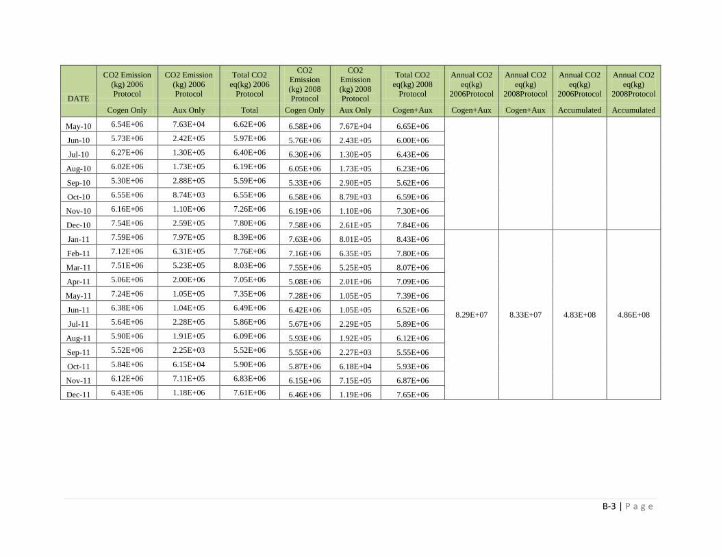
B-3 | P a g e

DATE

CO2 Emission

(kg) 2006

Protocol

CO2 Emission

(kg) 2006

Protocol

Total CO2

eq(kg) 2006

Protocol

CO2

Emission

(kg) 2008

Protocol

CO2

Emission

(kg) 2008

Protocol

Total CO2

eq(kg) 2008

Protocol

Annual CO2

eq(kg)

2006Protocol

Annual CO2

eq(kg)

2008Protocol

Annual CO2

eq(kg)

2006Protocol

Annual CO2

eq(kg)

2008Protocol


May-10 6.54E+06 7.63E+04 6.62E+06 6.58E+06 7.67E+04 6.65E+06

Jun-10 5.73E+06 2.42E+05 5.97E+06 5.76E+06 2.43E+05 6.00E+06

Jul-10 6.27E+06 1.30E+05 6.40E+06 6.30E+06 1.30E+05 6.43E+06

Aug-10 6.02E+06 1.73E+05 6.19E+06 6.05E+06 1.73E+05 6.23E+06

Sep-10 5.30E+06 2.88E+05 5.59E+06 5.33E+06 2.90E+05 5.62E+06

Oct-10 6.55E+06 8.74E+03 6.55E+06 6.58E+06 8.79E+03 6.59E+06

Nov-10 6.16E+06 1.10E+06 7.26E+06 6.19E+06 1.10E+06 7.30E+06

Dec-10 7.54E+06 2.59E+05 7.80E+06 7.58E+06 2.61E+05 7.84E+06

Jan-11 7.59E+06 7.97E+05 8.39E+06 7.63E+06 8.01E+05 8.43E+06

8.29E+07 8.33E+07 4.83E+08 4.86E+08

Feb-11 7.12E+06 6.31E+05 7.76E+06 7.16E+06 6.35E+05 7.80E+06

Mar-11 7.51E+06 5.23E+05 8.03E+06 7.55E+06 5.25E+05 8.07E+06

Apr-11 5.06E+06 2.00E+06 7.05E+06 5.08E+06 2.01E+06 7.09E+06

May-11 7.24E+06 1.05E+05 7.35E+06 7.28E+06 1.05E+05 7.39E+06

Jun-11 6.38E+06 1.04E+05 6.49E+06 6.42E+06 1.05E+05 6.52E+06

Jul-11 5.64E+06 2.28E+05 5.86E+06 5.67E+06 2.29E+05 5.89E+06

Aug-11 5.90E+06 1.91E+05 6.09E+06 5.93E+06 1.92E+05 6.12E+06

Sep-11 5.52E+06 2.25E+03 5.52E+06 5.55E+06 2.27E+03 5.55E+06

Oct-11 5.84E+06 6.15E+04 5.90E+06 5.87E+06 6.18E+04 5.93E+06

Nov-11 6.12E+06 7.11E+05 6.83E+06 6.15E+06 7.15E+05 6.87E+06

Dec-11 6.43E+06 1.18E+06 7.61E+06 6.46E+06 1.19E+06 7.65E+06

C-1 | P a g e

Appendix C – Sensitivity Analysis (Percent GHG Emission Change with Changing Percentage Steam Energy Generated for a

Certain Amount of Natural Gas Burned)

Gas Burned (Cogen only) 1.44E+07 MMBtu

Gas Burned (Aux only) 6.24E+05 MMBtu

Auxilliary Broiler

Efficiency: 75%

Emission Factor (New): 5.43E+01 kg CO2/MMBtu

Actual Total Emission

(2006-2011): 4.86E+05 MT CO2

1kWh = 3.41E-03 MMBTU

Steam Enthalpy 1.193 MMBTU/LB

% Steam Energy Generated CO2 Emission 2008

Protocol (MT CO2)

Actual GHG Emission

(2006-2011)

(MTCO2)

Percent Change

50% 3.92E+05 4.86E+05 -19%

51% 4.00E+05 4.86E+05 -18%

52% 4.08E+05 4.86E+05 -16%

53% 4.16E+05 4.86E+05 -14%

54% 4.24E+05 4.86E+05 -13%

55% 4.32E+05 4.86E+05 -11%

56% 4.39E+05 4.86E+05 -10%

57% 4.47E+05 4.86E+05 -8%

58% 4.55E+05 4.86E+05 -6%

59% 4.63E+05 4.86E+05 -5%

60% 4.71E+05 4.86E+05 -3%

61% 4.79E+05 4.86E+05 -1%

62% 4.86E+05 4.86E+05 0%

63% 4.94E+05 4.86E+05 2%

C-2 | P a g e

% Steam Energy Generated CO2 Emission 2008

Protocol (MT CO2)

Actual GHG Emission

(2006-2011)

(MTCO2)

Percent Change

64% 5.02E+05 4.86E+05 3%

65% 5.10E+05 4.86E+05 5%

-25%

-20%

-15%

-10%

-5%

0%

5%

10%

0

100,000

200,000

300,000

400,000

500,000

600,000

50% 55% 60% 65%

GH

G E

mis

sion

(M

T C

O2 e

q.)

% Steam Energy Generated

Sensitivity Analysis - CO2 Emission Variation due to Changing % Total

Energy in Steam

CO2

Emission

2008

Protocol (MT

CO2) Actual Total

Emission

(2006-2011):

Percent

Change

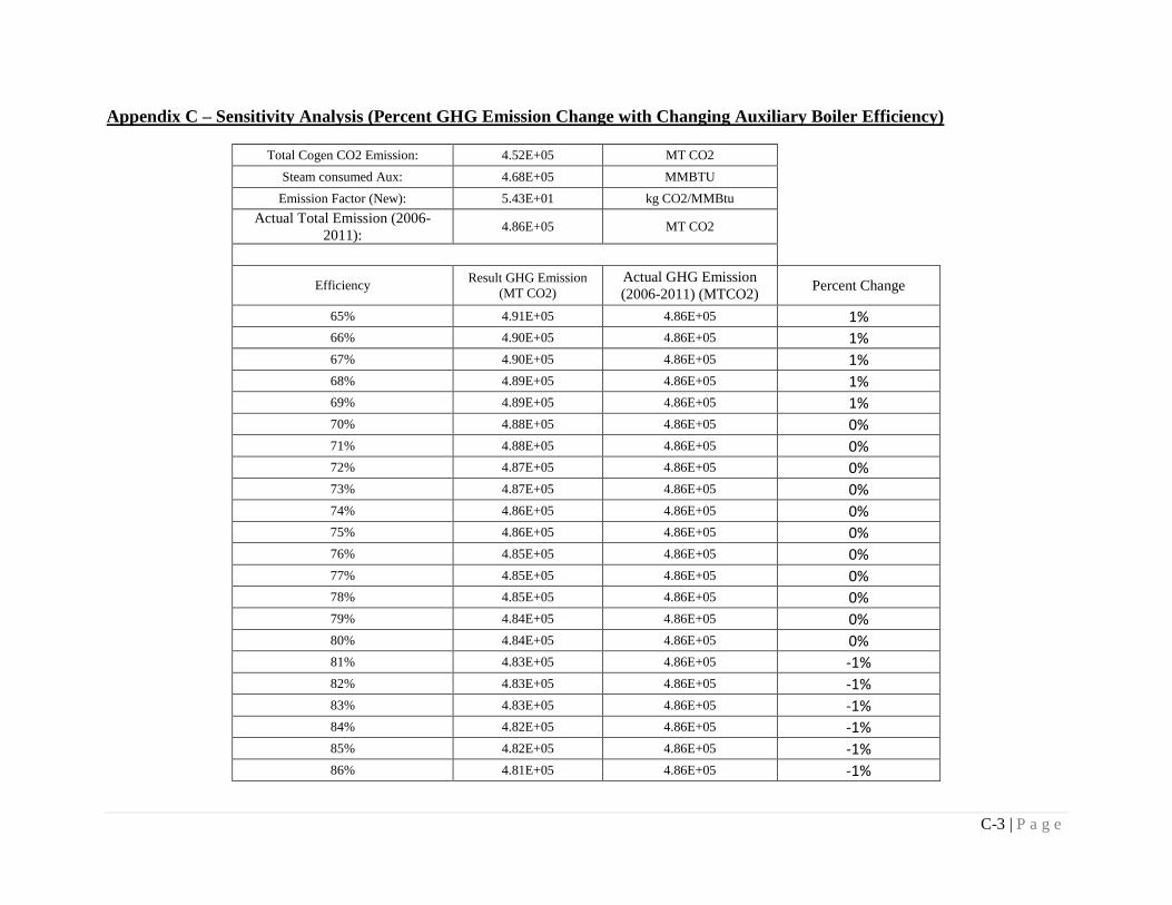
C-3 | P a g e

Appendix C – Sensitivity Analysis (Percent GHG Emission Change with Changing Auxiliary Boiler Efficiency)

Total Cogen CO2 Emission: 4.52E+05 MT CO2

Steam consumed Aux: 4.68E+05 MMBTU


Actual Total Emission (2006-

2011): 4.86E+05 MT CO2

Efficiency

Result GHG Emission

(MT CO2)

Actual GHG Emission

(2006-2011) (MTCO2) Percent Change

65% 4.91E+05 4.86E+05 1% 66% 4.90E+05 4.86E+05 1% 67% 4.90E+05 4.86E+05 1% 68% 4.89E+05 4.86E+05 1% 69% 4.89E+05 4.86E+05 1% 70% 4.88E+05 4.86E+05 0% 71% 4.88E+05 4.86E+05 0% 72% 4.87E+05 4.86E+05 0% 73% 4.87E+05 4.86E+05 0% 74% 4.86E+05 4.86E+05 0% 75% 4.86E+05 4.86E+05 0% 76% 4.85E+05 4.86E+05 0% 77% 4.85E+05 4.86E+05 0% 78% 4.85E+05 4.86E+05 0% 79% 4.84E+05 4.86E+05 0% 80% 4.84E+05 4.86E+05 0% 81% 4.83E+05 4.86E+05 -1% 82% 4.83E+05 4.86E+05 -1% 83% 4.83E+05 4.86E+05 -1% 84% 4.82E+05 4.86E+05 -1% 85% 4.82E+05 4.86E+05 -1% 86% 4.81E+05 4.86E+05 -1%

C-4 | P a g e

Efficiency Result GHG Emission

(MT CO2)

Actual GHG Emission

(2006-2011) (MTCO2) Percent Change

87% 4.81E+05 4.86E+05 -1% 88% 4.81E+05 4.86E+05 -1% 89% 4.81E+05 4.86E+05 -1% 90% 4.80E+05 4.86E+05 -1% 91% 4.80E+05 4.86E+05 -1% 92% 4.80E+05 4.86E+05 -1% 93% 4.79E+05 4.86E+05 -1% 94% 4.79E+05 4.86E+05 -1% 95% 4.79E+05 4.86E+05 -1%

-2.0%

-1.5%

-1.0%

-0.5%

0.0%

0.5%

1.0%

1.5%

472,000

477,000

482,000

487,000

492,000

497,000

65% 70% 75% 80% 85% 90% 95%

GH

G E

mis

sio

n (

MT

CO

2 e

q.)

Auxiliary Boiler Efficiency

Sensitivity Analysis - CO2 Emission Variation due to Changing

Auxilary Boiler Efficiency

Result GHG Emission (MT CO2)

Actual GHG Emission (2006-2011) (MTCO2)

Percent Change

C-5 | P a g e

Appendix C – Sensitivity Analysis (Percent GHG Emission Change with Changing Cogeneration Plant Efficiency)

Total Aux CO2 Emission: 6.24E+02 MT CO2

Steam consumed Cogen: 5.06E+06 MMBTU


Actual Total Emission (2006-

2011): 4.86E+05 MT CO2

Plant Design Efficiency: 52%

Cogen Power Efficiency

Result GHG Emission

(MT CO2)

Actual GHG Emission (2006-2011)

(MTCO2) Percent Change

50% 5.50E+05 4.86E+05 13%

51% 5.40E+05 4.86E+05 11%

52% 5.29E+05 4.86E+05 9%

53% 5.19E+05 4.86E+05 7%

54% 5.10E+05 4.86E+05 5%

55% 5.01E+05 4.86E+05 3%

56% 4.92E+05 4.86E+05 1%

57% 4.83E+05 4.86E+05 -1%

58% 4.75E+05 4.86E+05 -2%

59% 4.67E+05 4.86E+05 -4%

60% 4.59E+05 4.86E+05 -6%

61% 4.51E+05 4.86E+05 -7%

62% 4.44E+05 4.86E+05 -9%

63% 4.37E+05 4.86E+05 -10%

64% 4.30E+05 4.86E+05 -11%

65% 4.24E+05 4.86E+05 -13%

66% 4.17E+05 4.86E+05 -14%

67% 4.11E+05 4.86E+05 -15%

68% 4.05E+05 4.86E+05 -17%

69% 3.99E+05 4.86E+05 -18%

70% 3.93E+05 4.86E+05 -19%

71% 3.88E+05 4.86E+05 -20%

72% 3.82E+05 4.86E+05 -21%

73% 3.77E+05 4.86E+05 -22%

C-6 | P a g e

Cogen Power Efficiency Result GHG Emission

(MT CO2)

Actual GHG Emission (2006-2011)

(MTCO2) Percent Change

74% 3.72E+05 4.86E+05 -23%

75% 3.67E+05 4.86E+05 -24%

76% 3.62E+05 4.86E+05 -25%

77% 3.58E+05 4.86E+05 -26%

78% 3.53E+05 4.86E+05 -27%

79% 3.49E+05 4.86E+05 -28%

80% 3.44E+05 4.86E+05 -29%

81% 3.40E+05 4.86E+05 -30%

82% 3.36E+05 4.86E+05 -31%

83% 3.32E+05 4.86E+05 -32%

84% 3.28E+05 4.86E+05 -33%

85% 3.24E+05 4.86E+05 -33%

-40%

-30%

-20%

-10%

0%

10%

20%

0

100,000

200,000

300,000

400,000

500,000

600,000

50% 55% 60% 65% 70% 75% 80% 85% GH

G E

mis

sio

n (

MT

CO

2 e

q.)

Cogenerataion Plant Power Efficiency

Sensitivity Analysis - CO2 Emission Variation due to Changing

Cogeneration Plant Power Efficiency

Result GHG Emission (MT CO2)

Actual GHG Emission (MTCO2)

Percent Change

D-1 | P a g e

APPENDIX D – Heating Case Study

Energy Needed Per Building

Natural Gas Alternative

Pricing

Campus Average Rate

D-2 | P a g e

Cogeneration Plant Assumed Rate

Electricity Alternative

Electricity From PG&E

Emissions

Electricity From Cogeneration Plant

.

D-3 | P a g e

Emissions

Pricing

Steam Alternative

.

Emissions

D-4 | P a g e

Pricing

E-1 | P a g e

APPENDIX E – Cost and GHG Emissions for Autoclaves

Energy Needed Per Autoclave per year

(Narang Medial Limited, 2012).

Natural Gas Alternative

Pricing

Electricity Alternative

Electricity From PG&E

Emissions

Pricing

E-2 | P a g e

Conversion to pounds of steam consumed per month for easy comparison with graphs

STEAM EMISSIONS OF UC CAMPUS: MITIGATING CLIMATE IMPACTS · PDF fileSTEAM EMISSIONS OF UC...

Documents

Transcript of STEAM EMISSIONS OF UC CAMPUS: MITIGATING CLIMATE IMPACTS · PDF fileSTEAM EMISSIONS OF UC...