INTERNATIONAL JOURNAL OF PRECISION ENGINEERING AND MANUFACTURING Vol. 13, No. 6, pp. 927-933 JUNE 2012 / 927 DOI: 10.1007/s12541-012-0120-5

1. Introduction

When analyzing the vibration system composed of time-varying properties, it is needed to consider parametric vibration analysis. A typical example of these systems is a pipe system conveying pulsating fluid.1,2 The equation of motion for these systems was derived by Païdoussis. According to this equation, the properties of pipe system such as stiffness and damping are time-dependent terms caused by the pulsation.1 This system is a typical example of parametric vibration excited by time varying coefficients. Many researches have been studied to analyze parametrically excited system.

Several method to compute the steady-state response of linear systems with periodically varying parameters under external excitations was researched.3-7 Hsu presented an explicit expression for steady-state periodic response of a such a system given in terms of the fundamental matrix of the homogeneous system.3 Farhang suggested direct method to evaluate the steady-state response of periodically time-varying linear systems and demonstrated its efficacy through the application to a high-speed elastic mechanism.4 Selstad also suggested the method to solve the stead-state response of these system by dividing the fundamental

period into a number of intervals and establishing the response at the start and end of the period.5 Perret proposed the interactive spectral method based on the modal approach which is developed on the frequency domain to calculate the steady state forced response.6 Deltombe used direct spectral method to analyze the parametric system forced response on frequency domain and showed the reliability of the method.7

In case of linear slowly varying system under external excitation, Shahruz derived approximate closed-form solution by using the technique of freezing slowly varying parameters.8

For the stability analysis of linear systems with periodic parameters, Sinha used a new efficient numerical scheme based on the idea that the state vector and the periodic matrix of the system can be expanded in terms of Chebyshev polynomials over the principal period.9

Recently, some researches to analyze the beam and various method to obtain properties of beam were implemented. Lughmni studied the bending behavior of beam by establishing FEM modeling and experiment.10 Kim suggested a method to find Poisson’s ratio of cantilever beam by using holographic technique.11

The literatures mentioned above showed the advantage in analysis on frequency domain but relatively not much research has

Steady-state Vibration Analysis of Modal Beam Model under Parametric Excitation

Seong-Hyeon Lee1 and Weui-Bong Jeong1,# 1 School of Mechanical Engineering, Pusan National University, San 30, Jangjeon-dong, Geumjeong-gu, Busan, South Korea, 609-735

# Corresponding Author / E-mail: wbjeong@pusan.ac.kr, TEL: +82-51-510-2337, FAX: +82-51-517-3805

KEYWORDS: Beam model, Numerical time domain analysis, Parametric excitation, Steady-state vibration, Time-varying system

This research suggests the efficient numerical scheme to analyze the time-response of steady-state vibration of modal beam model when the properties (stiffness, damping) of the model are time-varying. The piping system conveying harmonically pulsating fluid is a typical example of parametrically excited system because the properties such as stiffness and damping are time-dependent characteristics. To analyze the time-response of this system, numerical integration method of differential equations, such as the Runge-Kutta method was usually used. But this method requires extensive computational efforts to solve the time-response of time-varying systems. In this paper, the governing equation was transformed to a single degree-of-freedom model at a certain mode by using assumed-mode method. A new method to predict efficiently the steady-state response for a time-varying system was presented. The steady-state response was assumed to have the frequency of the pulsation and its multiples, and was predicted by comparing the coefficients of Taylor series expansion. The efficiency of this method was validated by the comparison with conventional numerical method of differential equations and experimental results.

Manuscript received: April 14, 2011 / Accepted: December 29, 2011

© KSPE and Springer 2012

928 / JUNE 2012 INTERNATIONAL JOURNAL OF PRECISION ENGINEERING AND MANUFACTURING Vol. 13, No. 6 been done on the prediction of the time-historied response of these systems. Usually a reliable displacement response with respect to time can be obtained only by very time-consuming calculation.

In this paper, an efficient time domain method to predict the steady-state response of a parametrically excited system is presented. For this analysis, the equation of motion of the pipe system suggested by Païdoussis1 was assumed as single-degree-of-freedom modal beam. The steady-state response is assumed to have the frequency of the pulsation in the pipes and its multiples. The amplitude and phase of the steady-state response are estimated from a simultaneous equation, which is derived by comparing the coefficients of a Taylor series expansion.

2. Modal beam model under parametric excitation When analyzing the vibration system composed of time-varying

properties, it is needed to consider parametric vibration analysis. A typical example of these systems is a pipe system conveying pulsating fluid.1,2 The equation of motion for these systems was derived by Païdoussis. According to this equation, the properties of pipe system such as stiffness and damping are time-dependent terms caused by the pulsation.1 This system is a typical example of parametric vibration excited by time varying coefficients. Many researches have been studied to analyze parametrically excited system.

The governing equation of the piping system conveying the fluid is derived by Païdoussis as equation (1).13,14

( ) ( ) ( ) ( ) ( )

( ) ( ) ( )

4 2 22

4 2

2

2

, , ,2

,,

f f

f

y x t y x t y x tEI AU t AU t

x x x ty x t

m A p x tt

ρ ρ

ρ

∂ ∂ ∂+ +

∂ ∂ ∂ ∂∂

+ + =∂

(1)

Here, ρf , and U(t) are fluid density and velocity, p(x,t) is distributed force and A is cross-section area of a pipe. The Young’s modulus, area moment of inertia and mass per unit length of this pipe are represented as E, I and m respectively.

The equation (1) can be expressed in variational form like equation (2)

( ) ( ) ( )

( ) ( ) ( ) ( )

2

1

4 2 22

4 20

2

2

, , ,2

,, , 0

t l

f ft

f

y x t y x t y x tEI AU AU

x x x t

y x tm A p x t y x t dxdt

t

ρ ρ

ρ δ

⎡ ∂ ∂ ∂+ +⎢

∂ ∂ ∂ ∂⎣⎤∂

+ + − =⎥∂ ⎦

∫ ∫ (2)

Let us assume the transverse displacement as follows.

( ) ( ) ( ),y x t w x q t= (3)

where w(x) and q(t) represent the assumed-mode shape and modal coordinate. If the response in modal coordinate is obtained, the response in physical coordinate can be also obtained by the superposition of modes.15

Substitution of equation (3) into equation (2) and integration by parts leads to

( ) ( ) ( )

( ) ( ){ } ( )

( ) ( ) ( ) ( ) ( ) ( )

2

1

2

1

2 2222

2

02 2

0

12

12

2 , 0

ft l

t

f

t l

ft

d w x dw xEI AU q t

dx dx dxdt

m A w x q t

dw xAUw x q t w x p x t q t dxdt

dx

ρδ

ρ

ρ δ

⎡ ⎤⎧ ⎫⎡ ⎤ ⎡ ⎤⎪ ⎪⎢ ⎥−⎨ ⎬⎢ ⎥ ⎢ ⎥⎢ ⎥⎣ ⎦⎣ ⎦⎪ ⎪⎩ ⎭⎢ ⎥⎢ ⎥− +⎢ ⎥⎣ ⎦

⎡ ⎤⎧ ⎫⎪ ⎪+ − =⎢ ⎥⎨ ⎬⎪ ⎪⎢ ⎥⎩ ⎭⎣ ⎦

∫ ∫

∫ ∫

&

&

(4)

On the other hand, Hamilton’s principle is given by

( )2 2

1 1

0t t

nct tT V dt W dtδ δ− + =∫ ∫ (5)

where

( )212 eqT m q t= & (6)

( )212 eqV k q t= (7)

δWnc represents the virtual work done by nonconservative forces such as the damping force proportional to the velocity ( )q t& and external force. And meq and keq are equilibrium mass and equilibrium stiffness, respectively.

Comparing equation (4) with equation (5), the equation of motion with a single degree-of-freedom system can be derived as the following form.

( ) ( ) ( ) ( ) ( )( ) ( ) ( )s f f s f extm m q t C t q t K K t q t f t+ + + − =&& & (8)

where fext(t) is the external force due to pulsation, ms and Ks are the mass and the stiffness of the pipe, given by equation (9) and (10).

( ) 22

20

l

s

d w xK EI dx

dx⎡ ⎤

= ⎢ ⎥⎣ ⎦

∫ (9)

( )2

0

l

sm mw x dx= ∫ (10)

mf is the mass of fluid in a pipe, Cf (t) and Kf (t) are the time-varying damping and stiffness due to the fluid. The Kf (t), Cf (t) and mf are given by equations (11), (12), and (13).

( ) ( )2f fK t A U tρ α= (11)

( ) ( )2f fC t A U tρ β= (12)

( )2

0

l

f fm Aw x dxρ= ∫ (13)

U(t) represents the velocity. The α and β are the constant values obtained from the integration of the assumed-mode w(x) in equation (4) as follows.

2

0

( )l dw x dxdx

α ⎡ ⎤= ⎢ ⎥⎣ ⎦∫ (14)

( ) ( )0

l dw xw x dx

dxβ = ∫ (15)

INTERNATIONAL JOURNAL OF PRECISION ENGINEERING AND MANUFACTURING Vol. 13, No. 6 JUNE 2012 / 929

3. Analysis method Let us assume harmonically pulsating velocity is given by

equation (16).

( ) ( )0 1 sin fU t U U tω= + (16)

where U0 is the mean velocity, U1 is the amplitude and ωf is pulsating frequency. The external distributed force due to the pulsation will have the same frequency with that of pulsation such as p(x,t) = P(x)sin(ωf t). The external force in equation (8) can be represented as follows.

( ) ( ) ( )0

, sinl

ext ext ff t w x p x t dx F tω= =∫ (17)

Substituting equation (16) into equation (12), Cf (t) becomes equation (18).

( ) ( )( )( )

( )( )0 1

2

2 sin

1 sin

f f

f f

u f

C t A U t

A U U t

C t

ρ β

ρ β ω

ε ω

=

= +

= +

(18)

where

02 fC A Uρ β= (19)

1

0u

UU

ε = (20)

C denotes the mean value of the fluctuating damping coefficient and εu denotes the ratio of the pulsating amplitude to the mean velocity. Rearranging equation (11) using the equation (16) leads to equation (21).

( ) ( ) ( )2 21 11 2 sin cos 22 2f u f u u fK t K t tε ω ε ε ω⎛ ⎞= + + −⎜ ⎟

⎝ ⎠ (21)

where K is 20 ,A Uρ α which represents the mean value of the time-

varying stiffness. By substituting M for ms+mf, Cf (t) for equation (18) and Kf (t) for equation (21), equation (8) can be written as equation (22).

( ) ( ) ( )

( )2

2

1 sin( )

11 2 sin( )2

1 cos(2 )2

sin( )

u f

u f u

s

u f

f

Mx t C t x t

tK K x t

t

F t

ε ω

ε ω ε

ε ω

ω

+ +

⎛ ⎞⎛ ⎞+ +⎜ ⎟⎜ ⎟⎜ ⎟⎜ ⎟+ −⎜ ⎟⎜ ⎟−⎜ ⎟⎜ ⎟⎝ ⎠⎝ ⎠

=

&& &

(22)

By using the 4th Runge-Kutta method, one of the popular differential equation analysis method, the displacement x(t) of equation (22) was obtained. The analysis condition of this equation is given by Table 1.

Fig. 1 shows the Fourier transformed spectrum of x(t) for sampling time 0.0032s. In Fig. 1, x(t) is composed of the fundamental pulsating frequency and the harmonic terms. The continuous frequency components except the harmonics can be ignored since it is caused by the leakage error. Therefore, displacement x(t) can be assumed to have the form of equation (23).

Table 1 Analysis condition of equation (22) for Runge-Kutta method ms 1 mf 0.05 ρA 100 U0 1 U1 0.1 Ks 10000 F 1 ωf 2·π·10 Δt 0.0032/28

0 10 20 3010-9

10-8

10-7

10-6

10-5

10-4

10-3

Am

plitu

deFrequency [Hz]

Fig. 1 FFT graph of x(t) solved by 4th Runge-Kutta method

( ) ( ){ }1

( ) cos sinN

n f n fn

x t A n t B n tω ω=

= +∑ (23)

Substituting equation (23) into equation (22) leads to the following equation.

( ) ( )( ) ( )

( )( ) ( ) ( )( ) ( )

( )( )

( ) ( ){ }

2

2

2 2

cos

sin

sin1 sin

cos

1 2 sin

1 1 cos 22 2

cos sin

sin

n f f

n f f

n f f

u f

n f f

u f

s

u u f

n f n f

A n n tM

B n n t

A n n tC t

B n n t

tK K

t

A n t B n t

F

ω ω

ω ω

ω ωε ω

ω ω

ε ω

ε ε ω

ω ω

⎡ ⎤⎧ ⎫−⎪ ⎪⎢ ⎥⎨ ⎬⎢ ⎥⎪ ⎪−⎢ ⎥⎩ ⎭⎢ ⎥

⎧ ⎫−⎢ ⎥⎪ ⎪+ +⎢ ⎥⎨ ⎬+⎢ ⎥⎪ ⎪⎩ ⎭⎢ ⎥

⎢ ⎥⎛ ⎞⎛ ⎞+⎜ ⎟⎢ ⎥⎜ ⎟+ −⎜ ⎟⎢ ⎥⎜ ⎟

+ −⎜ ⎟⎜ ⎟⎢ ⎥⎝ ⎠⎝ ⎠⎢ ⎥⎢ ⎥+⎢ ⎥⎣ ⎦

= ( )

1

N

n

f tω

=∑ (24)

The trigonometric function terms of equation (24), like sin(ωft), sin(nωft) and cos(nωft), can be approximated by Taylor series as follows.

( ) ( ) ( )3 5

sin3! 5!

f ff f

n t n tn t n t

ω ωω ω= − + K (25-1)

( ) ( ) ( )2 4

cos 12! 4!

f ff

n t n tn t

ω ωω = − + K (25-2)

After replacing the trigonometric terms with Taylor series terms, equation (24) can be rearranged in terms of the (ωft)n. Comparing the coefficients of (ωft)i, (i=0,1,2,…m) of both sides of equation (24), the matrix form of the simultaneous equations of this system can be derived as follows.

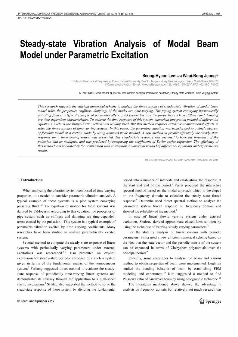
930 / JUNE 2012 INTERNATIONAL JOURNAL OF PRECISION ENGINEERING AND MANUFACTURING Vol. 13, No. 6 [ ]{ } { }D AB Force= (26)

where

{ } { }1 2 1 2 2 1

Tm m m

AB A A A B B B×

= L L (27)

{ } ( )( ) ( )( )

( )

1 1 1

2 1

1 10 0

1! 2 1 !

Tm

m

Forcem

− −

×

⎧ ⎫− −⎪ ⎪= ⎨ ⎬−⎪ ⎪⎩ ⎭

L (28)

2m×2m matrix [D] can be obtained by comparing the coefficients of left and right-hand sides. By solving equation (26), the coefficients of equation (27) can be calculated. Using this result, the assumed displacement, represented by equation (23), can be obtained.

4. Analysis and validation of developed method

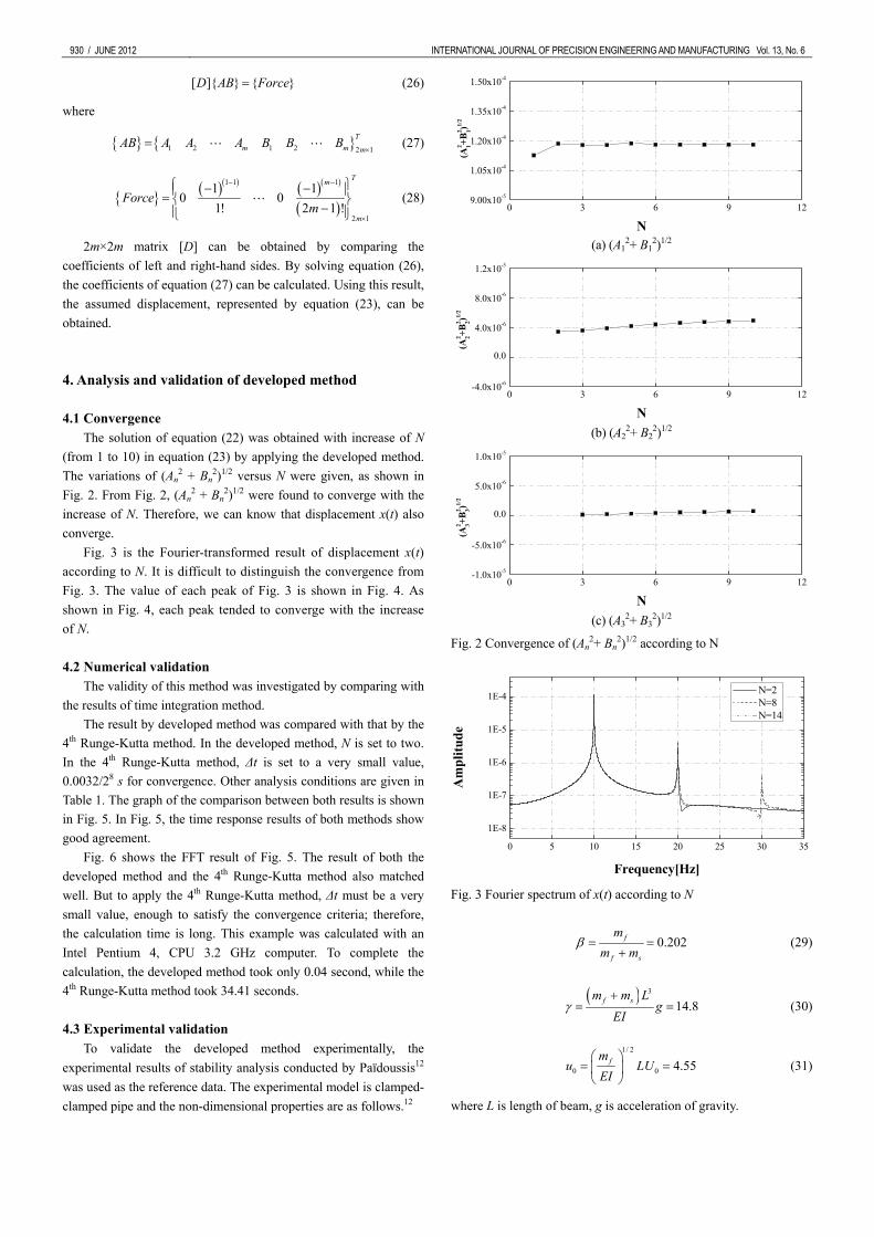
4.1 Convergence The solution of equation (22) was obtained with increase of N

(from 1 to 10) in equation (23) by applying the developed method. The variations of (An

2 + Bn2)1/2 versus N were given, as shown in

Fig. 2. From Fig. 2, (An2 + Bn

2)1/2 were found to converge with the increase of N. Therefore, we can know that displacement x(t) also converge.

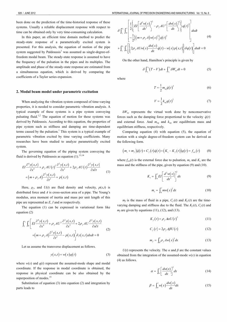
Fig. 3 is the Fourier-transformed result of displacement x(t) according to N. It is difficult to distinguish the convergence from Fig. 3. The value of each peak of Fig. 3 is shown in Fig. 4. As shown in Fig. 4, each peak tended to converge with the increase of N.

4.2 Numerical validation

The validity of this method was investigated by comparing with the results of time integration method.

The result by developed method was compared with that by the 4th Runge-Kutta method. In the developed method, N is set to two. In the 4th Runge-Kutta method, Δt is set to a very small value, 0.0032/28 s for convergence. Other analysis conditions are given in Table 1. The graph of the comparison between both results is shown in Fig. 5. In Fig. 5, the time response results of both methods show good agreement.

Fig. 6 shows the FFT result of Fig. 5. The result of both the developed method and the 4th Runge-Kutta method also matched well. But to apply the 4th Runge-Kutta method, Δt must be a very small value, enough to satisfy the convergence criteria; therefore, the calculation time is long. This example was calculated with an Intel Pentium 4, CPU 3.2 GHz computer. To complete the calculation, the developed method took only 0.04 second, while the 4th Runge-Kutta method took 34.41 seconds.

4.3 Experimental validation

To validate the developed method experimentally, the experimental results of stability analysis conducted by Païdoussis12 was used as the reference data. The experimental model is clamped-clamped pipe and the non-dimensional properties are as follows.12

0 3 6 9 129.00x10-5

1.05x10-4

1.20x10-4

1.35x10-4

1.50x10-4

(A2 1+B

2 1)1/2

N (a) (A1

2+ B12)1/2

0 3 6 9 12-4.0x10-6

0.0

4.0x10-6

8.0x10-6

1.2x10-5

(A2 2+B

2 2)1/2

N (b) (A2

2+ B22)1/2

0 3 6 9 12-1.0x10-5

-5.0x10-6

0.0

5.0x10-6

1.0x10-5

(A2 3+B

2 3)1/2

N (c) (A3

2+ B32)1/2

Fig. 2 Convergence of (An2+ Bn

2)1/2 according to N

0 5 10 15 20 25 30 35

1E-8

1E-7

1E-6

1E-5

1E-4

Am

plitu

de

Frequency[Hz]

N=2 N=8 N=14

Fig. 3 Fourier spectrum of x(t) according to N

0.202f

f s

mm m

β = =+

(29)

( ) 3

14.8f sm m Lg

EIγ

+= = (30)

1/ 2

0 0 4.55fmu LU

EI⎛ ⎞

= =⎜ ⎟⎝ ⎠

(31)

where L is length of beam, g is acceleration of gravity.

INTERNATIONAL JOURNAL OF PRECISION ENGINEERING AND MANUFACTURING Vol. 13, No. 6 JUNE 2012 / 931

0 5 10 15 201.12x10-4

1.13x10-4

1.14x10-4

1.15x10-4

1.16x10-41s

t pea

k

N (a) 1st peak

0 5 10 15 20-4.0x10-6

0.0

4.0x10-6

8.0x10-6

1.2x10-5

2nd

peak

N (b) 2nd peak

0 5 10 15 20-3.00x10-6

-1.50x10-6

0.00

1.50x10-6

3.00x10-6

3rd

peak

N (c) 3rd peak

Fig. 4 Peak value of FFT result

0.1 0.2 0.3 0.4 0.5-3.00x10-4

-1.50x10-4

0.00

1.50x10-4

3.00x10-4

X(t)

Time

Developed method 4th Runge-Kutta method

Fig. 5 Time response result of developed method and 4th Runge-Kuta method

In this experiment,12 the displacement for the principal

parametric resonance is expressed by assuming “n=1/2, 3/2, 5/2, ···” in equation (23). The displacement for the fundamental parametric resonance is also expressed by assuming “n=1, 2, 3, ···”.

The experimental result of first-mode principal and fundamental parametric resonances suggested by Païdoussis were shown in Figs. 7 and 8 along with the results of developed method.

0 5 10 15 20 25 30 3510-8

10-7

10-6

10-5

10-4

10-3

Developed method 4th Runge-Kutta method

Am

plitu

de

Frequency[Hz] Fig. 6 FFT result of Fig. 5

0.0 0.1 0.2 0.3 0.4 0.50

10

20

30

40

50 experiment developed method

ω*

εu

Fig. 7 Experimental boundaries of the first-mode principal parametric resonance compared with developed method, for a clamped-clamped pipe

0.0 0.1 0.2 0.3 0.4 0.50

10

20

30

40

50 experiment developed method

ω*

εu Fig. 8 Experimental boundaries of the first-mode fundamental parametric resonance compared with developed method, for a clamped-clamped pipe

From Figs. 7 and 8, the stability boundaries calculated by the

developed method showed good agreement with the experimental results.

The non-dimensional frequency ω* in Figs. 7 and 8 has the relation as equation (32).

1/ 2

3* f sf

m mL

EIω ω

+⎛ ⎞= ⎜ ⎟

⎝ ⎠ (32)

4.4 The effects of the pulsating terms

Equation (22) can be expressed as equation (33).

932 / JUNE 2012 INTERNATIONAL JOURNAL OF PRECISION ENGINEERING AND MANUFACTURING Vol. 13, No. 6 Table 2 Analysis condition for equation (36)

ρA 100 Ks 1.0×104 ωf 2·π·10 εu 0< εu ≤0.4 εk 0< εk ≤0.04

( ) ( )( ){ } ( )

( )( )( )

( )

( )

2

2 2

2 1 sin

1 2sin1 1 1 cos 2

2 2

sin

n f u

f u

n k

u f u

f

x t t x t

tx t

t

F tM

ζω ω ε

ω εω ε

ε ω ε

ω

+ +

⎡ ⎤⎧ ⎫+⎢ ⎥⎪ ⎪

+ −⎢ ⎥⎨ ⎬⎛ ⎞⎢ ⎥+ −⎪ ⎪⎜ ⎟⎢ ⎥⎝ ⎠⎩ ⎭⎣ ⎦

=

&& &

(33)

where

2

0k

s s

K AUK K

ρε = = (34)

2 nCM

ζω = (35)

2 sn

KM

ω = (36)

Here, εk represents the ratio of stiffness due to the pulsation with mean velocity U0 to the structural stiffness. ωn denotes the natural frequency of the pipe structure with stationary fluid. ζ denotes the damping ratio. The εu was already defined in equation (20).

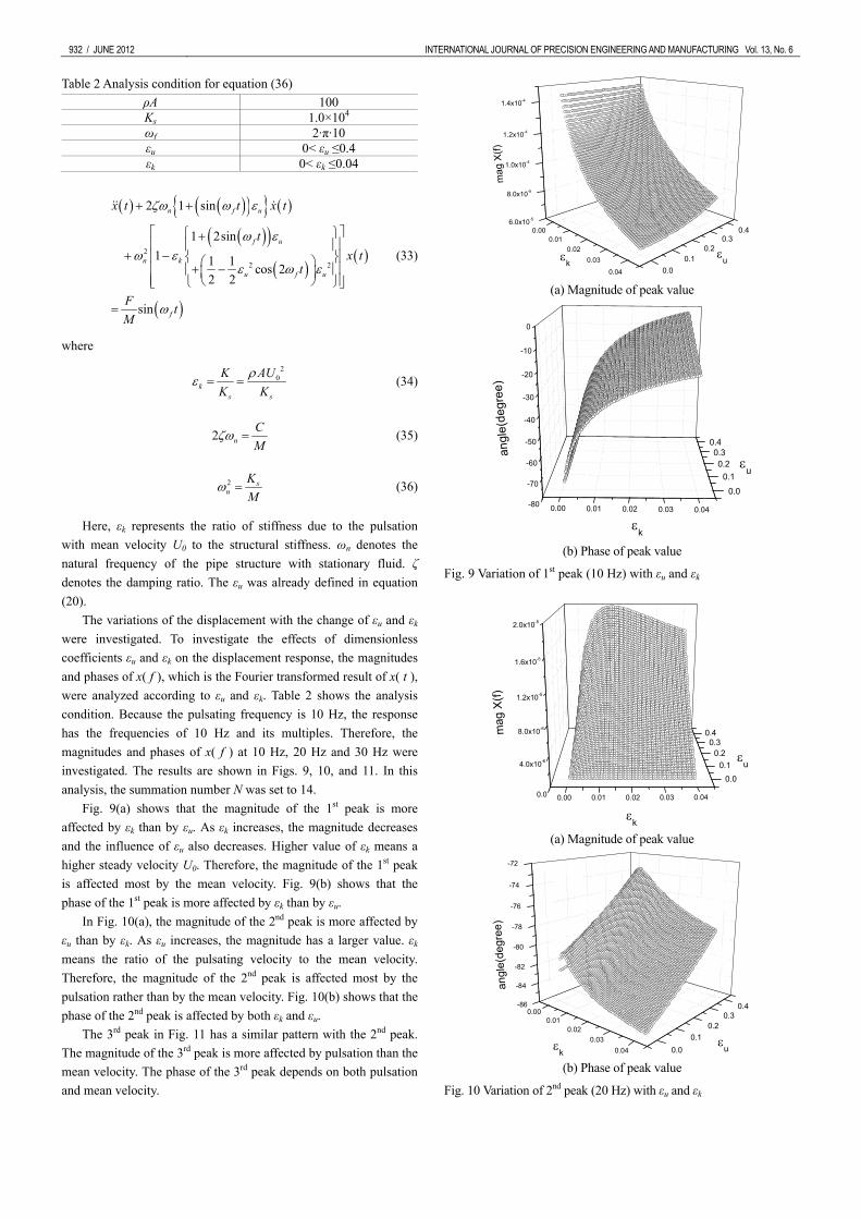
The variations of the displacement with the change of εu and εk were investigated. To investigate the effects of dimensionless coefficients εu and εk on the displacement response, the magnitudes and phases of x( f ), which is the Fourier transformed result of x( t ), were analyzed according to εu and εk. Table 2 shows the analysis condition. Because the pulsating frequency is 10 Hz, the response has the frequencies of 10 Hz and its multiples. Therefore, the magnitudes and phases of x( f ) at 10 Hz, 20 Hz and 30 Hz were investigated. The results are shown in Figs. 9, 10, and 11. In this analysis, the summation number N was set to 14.

Fig. 9(a) shows that the magnitude of the 1st peak is more affected by εk than by εu. As εk increases, the magnitude decreases and the influence of εu also decreases. Higher value of εk means a higher steady velocity U0. Therefore, the magnitude of the 1st peak is affected most by the mean velocity. Fig. 9(b) shows that the phase of the 1st peak is more affected by εk than by εu.

In Fig. 10(a), the magnitude of the 2nd peak is more affected by εu than by εk. As εu increases, the magnitude has a larger value. εk means the ratio of the pulsating velocity to the mean velocity. Therefore, the magnitude of the 2nd peak is affected most by the pulsation rather than by the mean velocity. Fig. 10(b) shows that the phase of the 2nd peak is affected by both εk and εu.

The 3rd peak in Fig. 11 has a similar pattern with the 2nd peak. The magnitude of the 3rd peak is more affected by pulsation than the mean velocity. The phase of the 3rd peak depends on both pulsation and mean velocity.

0.000.01

0.020.03

0.04

6.0x10-5

8.0x10-5

1.0x10-4

1.2x10-4

1.4x10-4

0.00.1

0.20.3

0.4

mag

X(f)

εuεk

(a) Magnitude of peak value

0.00 0.01 0.02 0.03 0.04-80

-70

-60

-50

-40

-30

-20

-10

0

0.0

0.10.2

0.30.4

εk

εu

angl

e(de

gree

)

(b) Phase of peak value

Fig. 9 Variation of 1st peak (10 Hz) with εu and εk

0.00 0.01 0.02 0.03 0.040.0

4.0x10-6

8.0x10-6

1.2x10-5

1.6x10-5

2.0x10-5

0.00.1

0.20.3

0.4

εu

εk

mag

X(f)

(a) Magnitude of peak value

0.000.01

0.020.03

0.04

-86

-84

-82

-80

-78

-76

-74

-72

0.00.1

0.20.3

0.4

angl

e(de

gree

)

εkεu

(b) Phase of peak value

Fig. 10 Variation of 2nd peak (20 Hz) with εu and εk

INTERNATIONAL JOURNAL OF PRECISION ENGINEERING AND MANUFACTURING Vol. 13, No. 6 JUNE 2012 / 933

0.00 0.01 0.02 0.03 0.040.0

4.0x10-6

8.0x10-6

1.2x10-5

1.6x10-5

2.0x10-5

0.00.1

0.20.3

0.4

εu

εk

mag

X(f)

(a) Magnitude of peak value

0.000.01

0.020.03

0.04

-86

-84

-82

-80

-78

-76

-74

-72

0.00.1

0.20.3

0.4

angl

e(de

gree

)

εkεu

(b) Phase of peak value

Fig. 11 Variation of 3rd peak (30 Hz) with εu and εk

5. Conclusions

The equation of motion for the transverse motion of a piping

system conveying pulsating fluid, having time-varying stiffness and damping characteristics, was modeled as a single degree-of-freedom at a certain mode by using the assumed-mode method. An efficient method to predict the steady-state response was presented by assuming that the steady-state response has the frequencies of pulsation and its multiples. Comparing the results by the proposed method with those by conventional numerical time-domain method, the accuracy and computational efficiency of the proposed method was verified. The boundaries of stability obtained by the proposed method showed good agreement with Païdoussis’s experimental results.12 The effects of dimensionless coefficients on steady state response were also investigated.

REFERENCES

1. Païdoussis, M. P. and Issid, N. T., “Dynamic stability of pipes conveying fluid,” Journal of Sound and Vibration, Vol. 33, No. 3, pp. 267-294, 1974.

2. Zhang, Y. L., Gorman, D. G., and Reese, J. M., “Analysis of the vibration of pipes conveying fluid,” Proceedings of the Institution of Mechanical Engineers Part C: Journal of

Mechanical Engineering Science, Vol. 213, No. 8, pp. 849-859, 1999.

3. Hsu, C. S. and Cheng, W.-H., “Steady-State Response of a Dynamical System Under Combined Parametric and Forcing Excitations,” Journal of Applied Mechanics, Vol. 41, No. 2, pp. 371-378, 1974.

4. Farhang, K. and Midha, A., “Steady-State Response of Periodically Time-Varying Linear Systems, With Application to an Elastic Mechanism,” Journal of Mechanical Design, Vol. 117, No. 4, pp. 633-639, 1995.

5. Selstad, T. J. and Farhang, K., “On Efficient Computation of the Steady-State Response of Linear Systems with Periodic Coefficients,” Journal of Vibration and Acoustics, Vol. 118, No. 3, pp. 522-526, 1996.

6. Perret-Liaudet, J., “An original method for computing the response of parametrically excited forced system,” Journal of Sound and Vibration, Vol. 196, No. 2, pp. 165-177, 1996.

7. Deltombe, R., Moraux, D., Plessis, G., and Level, P., “Forced response of structural dynamic systems with local time-dependent stiffnesses,” Journal of Sound and Vibration, Vol. 237, No. 5, pp. 761-773, 2000.

8. Shahruz, S. M. and Tan, C. A., “Response of linear slowly varying systems under external excitations,” Journal of Sound and Vibration, Vol. 131, No. 2, pp. 239-247, 1989.

9. Sinha, S. C. and Wu, D.-H., “An efficient computational scheme for the analysis of periodic systems,” Journal of Sound and Vibration, Vol. 151, No. 1, pp. 91-117, 1991.

10. Lughmani, W. A., Jho, J. Y., Lee, J. Y., and Rhee, K., “Modeling of Bending Behavior of IPMC Beams Using Concentrated Ion Boundary Layer,” Int. J. Precis. Eng. Manuf., Vol. 10, No. 5, pp. 131-139, 2009.

11. Kim, K. S., Chang, H. S., and Akhter, N., “Determination of Poisson’s Ratio of a Beam by Time-Average ESPI and Euler-Bernoulli Equation,” Int. J. Precis. Eng. Manuf., Vol. 11, No. 6, pp. 979-982, 2010.

12. Païdoussis, M. P. and Issid, N. T., “Experiments on Parametric Resonance of Pipes Containing Pulsatile Flow,” Journal of Applied Mechanics, Vol. 43, No. 2, pp. 198-203, 1976.

13. Païdoussis, M. P., “Fluid-Structure Interactions: Slender Structures and Axial Flow,” Academic Press, pp. 59-111, 1998.

14. Blevins, R. D., “Flow-Induced Vibration, 2nd ed.,” Van Nostrand Reinhold, pp. 384-392, 1990.

15. Rao, S. S., “Mechanical vibrations, 4th ed.,” Pearson Prentice Hall, pp. 542-577, 2004.